assessing the use of shrub-willows for living snow … for living snow fences in minnesota. ......

Assessing the Use of Shrub-Willows for Living

Snow Fences in Minnesota

Diomy Zamora, Principal InvestigatorUniversity of Minnesota Extension

November 2015

Research ProjectFinal Report 2015-46

To request this document in an alternative format call 651-366-4718 or 1-800-657-3774 (Greater Minnesota) or email your request to [email protected]. Please request at least one week in advance.

Technical Report Documentation Page 1. Report No. 2. 3. Recipients Accession No. MN/RC 2015-46 4. Title and Subtitle 5. Report Date

Assessing the Use of Shrub-Willows for Living Snow Fences in Minnesota

November 2015 6.

7. Author(s) 8. Performing Organization Report No. Diomy S Zamora, Eric Ogdahl, Gary Wyatt, David J. Smith, Gregg Johnson, Dean Current, Dan Gullickson,

9. Performing Organization Name and Address 10. Project/Task/Work Unit No. University of Minnesota Extension Center for Agriculture, Food and Natural Resources | Extension 227 Coffey Hall, 1420 Eckles Ave St. Paul, MN 55155-1899

CTS # 2014007 11. Contract (C) or Grant (G) No.

(c) 99008 (wo) 120

12. Sponsoring Organization Name and Address 13. Type of Report and Period Covered Minnesota Department of Transportation Research Services & Library 395 John Ireland Boulevard, MS 330 St. Paul, Minnesota 55155-1899

Final Report 14. Sponsoring Agency Code

15. Supplementary Notes http://www.lrrb.org/pdf/201546.pdf 16. Abstract (Limit: 250 words)

Blowing and drifting snow adversely affect winter driving conditions and road infrastructure in Minnesota, often requiring removal methods costly to the state and environment. Living snow fences (LSFs)—rows of trees, shrubs, grasses, or standing corn installed on fields upwind of roadways—are economically viable solutions for controlling drifting snow in agricultural areas. Despite incentives and financial assistance by state and federal agencies, farmer adoption of LSFs is low, in part due to concerns about removing cropland from production. Of recent interest in Minnesota is the use of shrub-willows (Salix spp.) for LSFs, as they have been successfully implemented for LSFs in other states and are researched increasingly as a marketable biomass product for bioenergy production. To evaluate the potential of willow LSFs for multiple benefits in Minnesota, we established studies in Waseca, Minnesota, 1) to test different designs of willow LSFs in their ability to trap snow, 2) to compare the growth of willow varieties to willows native to Minnesota and other species traditionally used in LSFs, and 3) to assess the costs of planting and establishing a willow snow fence and the viability of biomass harvest. We found all shrubs to have generally high survival rates, with willows tending to have higher growth than traditional LSF shrubs. Additionally, willow LSFs may have the potential to trap all blowing snow at the study site as soon as three to four years after planting. This may provide earlier road protection than other shrub species traditionally used in LSFs. Regarding economics, willows can provide affordable LSFs relative to traditional LSF species, although harvesting for biomass may only be appropriate for very long transportation corridors.

17. Document Analysis/Descriptors 18. Availability Statement Snow fences, Living things, Snowdrifts, Woody plants, Costs, Benefits

No restrictions. Document available from: National Technical Information Services, Alexandria, Virginia 22312

19. Security Class (this report) 20. Security Class (this page) 21. No. of Pages 22. Price Unclassified Unclassified 99

Assessing the Use of Shrub-Willows for Living Snow Fences in Minnesota

Final Report

Prepared by:

Diomy S. Zamora Eric Ogdahl Gary Wyatt

University of Minnesota Extension

David J. Smith Department of Applied Economics

University of Minnesota

Gregg Johnson Southern Research and Outreach Center


Dean Current Center for Integrated Natural Resources and Agricultural Management


Dan Gullickson Minnesota Department of Transportation

November 2015

Published by: Minnesota Department of Transportation

Research Services & Library 395 John Ireland Boulevard, MS 330

St. Paul, Minnesota 55155-1899 This report represents the results of research conducted by the authors and does not necessarily represent the views or policies of the Minnesota Department of Transportation or the University of Minnesota. This report does not contain a standard or specified technique. The authors and the Minnesota Department of Transportation and the University of Minnesota do not endorse products or manufacturers. Trade or manufacturers’ names appear herein solely because they are considered essential to this report.

ACKNOWLEDGMENTS

We acknowledge the University of Minnesota’s Southern Research and Outreach Center (SROC) for providing space for this research project and resources for maintaining the willow plantings. Special thanks goes to Tom Hoverstad, Paul Adams, and Matt Bickell of SROC for providing design, planting, and plot maintenance assistance during the establishment of this project. Additionally, we are grateful for Don Baker’s (MnDOT District 7) assistance in establishing and maintaining the project. We would also like to thank the local 4-H and Boy Scout groups for providing assistance during the planting and maintenance of the willow study sites. Field work assistance from Benjamin Katorosz and Alex Mehne is also greatly appreciated. We acknowledge the University of Minnesota’s Statistical Consulting Service for providing helpful suggestions during the design and analysis of this research. Thanks also goes to Justin Heavey and Tim Volk of State University of New York, College of Environmental Science and Forestry, and Martha Shulski of University of Nebraska, School of Natural Resources, for providing helpful suggestions and information on living snow fence research protocols. We thank Anna Dirkswager (MN DNR) and Kate MacFarland (USDA National Agroforestry Center) for providing information on biomass markets in Minnesota. Lastly, we thank state botanist Welby Smith, Minnesota Department of Natural Resources, for providing suggestions on appropriate native willows for living snow fences.

TABLE OF CONTENTS

Chapter 1: Establishment and Potential Snow Storage Capacity of Willow (Salix Spp.) Living Snow Fences in Waseca, Minnesota, USA ..................................................................................... 1

1.1 Abstract ................................................................................................................................. 1

1.2 Introduction ........................................................................................................................... 1

1.3 Materials and Methods .......................................................................................................... 3

1.3.1 Site description and experimental design ...................................................................... 3

1.3.2 Plant data collection ....................................................................................................... 4

1.3.3 Modeled snow storage capacity ..................................................................................... 6

1.3.4 Measured snow storage .................................................................................................. 7

1.3.5 Statistical analyses ......................................................................................................... 7

1.4 Results ................................................................................................................................... 8

1.4.1 Establishment and growth .............................................................................................. 8

1.4.2 Snow storage capacity.................................................................................................. 10

1.5 Discussion ........................................................................................................................... 13

1.6 Conclusion .......................................................................................................................... 16

Chapter 2: The Economics of Planting and Producing Biomass from Willow (Salix spp.) Living Snow Fences ................................................................................................................................. 18

2.1 Abstract ............................................................................................................................... 18

2.2 Introduction ......................................................................................................................... 18

2.3 Methods............................................................................................................................... 19

2.3.1 Planting and Establishment .......................................................................................... 19

2.3.2 Labor ............................................................................................................................ 20

2.3.3 Chemicals ..................................................................................................................... 21

2.3.4 Machinery .................................................................................................................... 21

2.3.5 Planting Stock .............................................................................................................. 22

2.3.6 Erosion Control ............................................................................................................ 23

2.3.7 Harvest ......................................................................................................................... 23

2.3.8 Transport ...................................................................................................................... 23

2.4 Results and Discussion ....................................................................................................... 24

2.4.1 Planting and Establishment .......................................................................................... 24

2.4.2 Conservation Program Cost Sharing ............................................................................ 25

2.4.3 Comparison to Current Living Snow Fence Costs ...................................................... 26

2.4.4 Biomass Production ..................................................................................................... 26

2.4.5 Enterprise Budgets ....................................................................................................... 27

2.4.6 Cash Flow .................................................................................................................... 27

2.4.7 Costs of Production ...................................................................................................... 27

2.4.8 Biomass facilities in Minnesota ................................................................................... 29

2.5 Conclusions and Implications ............................................................................................. 29

Chapter 3: Establishment and Growth of Native And Hybrid Shrub-Willows, Gray Dogwood, and American Cranberrybush for Use in Living Snow Fences .................................................... 32

3.1 Introduction ......................................................................................................................... 32

3.2 Methods............................................................................................................................... 32

3.2.1 Study site description ................................................................................................... 32

3.2.2 Experimental design and planting materials ................................................................ 33

3.2.3 Plant data collection ..................................................................................................... 35

3.2.4 Statistical analyses ....................................................................................................... 35

3.3 Results ................................................................................................................................. 35

3.3.1 Growth variables by species and year .......................................................................... 35

3.3.2 Effects of coppice timing on 2014 willow growth variables ....................................... 36

3.4 Discussion ........................................................................................................................... 37

3.5 Conclusion .......................................................................................................................... 39

Chapter 4: Conclusions ................................................................................................................. 40

4.1 Chapter 1 ............................................................................................................................. 40

4.2 Chapter 2 ............................................................................................................................. 40

4.3 Chapter 3 ............................................................................................................................. 41

References ..................................................................................................................................... 42

Snow Climatological Models for Waseca, Minnesota

Porosity Method for Adobe Photoshop CS Version 8.0

Biomass Facilities in Minnesota

Height And Porosity Assessment of a Living Snow Fence in Belle Plaine, Minnesota

Financial Assistance for Living Snow Fences In Minnesota

Photo Timeline of the Establishment and Growth of the Willow Living Snow Fence in Waseca, MN

LIST OF FIGURES

Figure 1.1: Example replicate of willow living snow fence experiment in Waseca, MN .............. 4 Figure 1.2: Using a large red backdrop to assess porosity in shrub-willow living snow fences .... 5 Figure 1.3: Mean heights for row positions in willow living snow fences with two- and four-row planting arrangements. Error bars represent 95% confidence intervals ......................................... 9 Figure 1.4: Selected porosity images that closely resemble the average porosity (in parentheses) for each willow variety and planting arrangement. Images presented do not necessarily imply statistical differences. .................................................................................................................... 10 Figure 1.5: Mean measured snow storage in willow living snow fences with two- and four-row planting arrangements. Different letters indicate significant difference under Tukey’s HSD test at P<0.001. Error bars show 95% confidence intervals ............................................................... 13 Figure 2.1: Number of active biomass facilities in Minnesota counties ....................................... 30 Figure 3.1: Example replicate for the comparison of candidate shrub species for living snow fences. All willows are represented by their common name provided in Table 3.2. "Native" refers to Salix petiolaris. ............................................................................................................... 34 Figure 3.2: American cranberrybush with wilted leaves and stems in June, 2014, shortly after herbicide application ..................................................................................................................... 38

LIST OF TABLES

Table 1.1: Selected soil characteristics for willow living snow fence establishment in Waseca, MN .................................................................................................................................................. 3 Table 1.2: Number of days with snowfall, rainfall, and above-freezing temperatures and the amount of snowfall during the 2014-2015 snow accumulation season at the Southern Research and Outreach Center in Waseca, Minnesota ................................................................................... 7 Table 1.3: Height, porosity, potential snow storage capacity (Qc) and ratio of Qc to mean annual snow transport (Q) for 6 willow living snow fence treatments after one growing season post-coppice. Values in parentheses are the standard error of the mean .............................................. 11 Table 1.4: Predicted height, porosity, potential snow storage capacity (Qc) and ratio of Qc to mean annual snow transport (Q) for two- and four-row willow snow fences at two, three, and four years after planting based on willow living snow fence models ........................................... 11 Table 1.5: Mean snow storage measurements in willow snow fences by number of rows and month during 2014-2015 winter ................................................................................................... 12 Table 2.1: Labor usage and costs for farm workers in Waseca, Minnesota during the willow living snow fence establishment ................................................................................................... 20 Table 2.2: Chemical usage, rates, and prices for Willow living snow fence establishment in Waseca, Minnesota ....................................................................................................................... 21 Table 2.3: Non-Harvest machinery, costs and hours for willow living snow fence establishment in Waseca, Minnesota ................................................................................................................... 22 Table 2.4: Planting stocks, replacement, and costs by willow variety based on planting arrangement designs...................................................................................................................... 23 Table 2.5: Harvest and transportation equipment cost of willow living snow fence in Waseca, Minnesota ...................................................................................................................................... 23 Table 2.6: Summary of per meter and total establishment costs for willow living snow fences in Minnesota, USA ............................................................................................................................ 25

Table 2.7: Reimbursement rates in US Dollars per hectare for two preparation methods and three previous vegetation types .............................................................................................................. 26 Table 2.8: EQIP cost share for 2- and 4-row willow living snow fences ..................................... 26 Table 2.9: Summaries of the total, per hectare and per meter costs for biomass production from a 454-meter 2- and 4-row and corridor-length willow living snow fence in Waseca, Minnesota .. 27 Table 2.10: Enterprise budget cash flow for willow living snow fence in 2- and 4-row arrangements. ................................................................................................................................ 28 Table 2.11: Summary of costs by net present value and annualized net present value for a 25-year stand life using 2- and 4-row planting arrangements and corridor-length willow living snow fences ............................................................................................................................................ 28 Table 2.12: Summary of annualized net present value of the 454-meter 2- and 4-row planting arrangement and the corridor-length willow living snow fences.................................................. 29 Table 3.1: Selected soil characteristics for shrub establishment at the University of Minnesota’s Agricultural Ecology Research Farm in Waseca, Minnesota ....................................................... 33 Table 3.2: Shrub species used in variety/species comparison study ............................................. 33 Table 3.3: Mean survival, heights, stem counts, and stem diameters for shrub-willows and traditional living snow fence shrubs in 2013 and 2014. ............................................................... 36 Table 3.4: The effect of coppice time and species on 2014 mean willow height and number of stems per plant. ............................................................................................................................. 37

EXECUTIVE SUMMARY

Blowing and drifting snow adversely affect winter driving conditions and road infrastructure in Minnesota, often requiring removal methods costly to the state and environment. Living snow fences (LSFs)—rows of trees, shrubs, grasses, or standing corn installed in fields upwind of roadways—are economically viable solutions for controlling drifting snow in agricultural areas. LSFs are an agroforestry practice and can provide a range of environmental benefits, including wildlife habitat and carbon sequestration. However, they often require multiple years to become effective and their adoption by landowners is relatively low, despite incentives and financial assistance by state and federal agencies. In Minnesota, for example, approximately 1,200 miles (1,930 km) of state roadways have severe blowing snow problems, but only 20 miles (30 km) have been addressed through landowner adoption of LSFs. Landowners have cited multiple barriers to LSF adoption, including removing cropland from production, hassle and time spent installing LSFs, and risk of plant mortality. Therefore, to improve LSF adoption, it is necessary to evaluate plants that are easily established and may provide landowners with a marketable product.

Shrub-willows (Salix spp.) have been developed as a short-rotation woody crop (SRWC) and proposed as a suitable LSF candidate. They are easily planted with dormant stem cuttings, have fast growth rates, offer a marketable product as a biomass crop, are adaptable to an array of site and climatic conditions, and offer numerous ecosystem services, such as pollinator habitat and carbon sequestration. Additionally, shrub-willows have potential to achieve key growth parameters for controlling blowing snow sooner than species traditionally used in LSFs. Previous research has shown shrub-willows can provide effective LSFs as soon as three years after planting, whereas other deciduous and coniferous species may require 5 to 20 years before providing effective LSFs. Overall, however, little has been done to assess the use of shrub-willows for LSFs, especially in Minnesota. To evaluate the potential of willow LSFs for multiple benefits in Minnesota, this project sought to determine appropriate willow variety selection and LSF planting designs in relation to trapping blowing snow, as well as evaluate the economics of planting and producing biomass from willow LSFs.

In the first part of this research (Chapter 1), we evaluated appropriate willow LSF designs in a demonstration LSF on a MnDOT right-of-way adjacent to US Highway 14 in Waseca, Minnesota. The LSF was planted in spring 2013 with three willow varieties in planting arrangements of two and four rows and replicated four times. We assessed willow establishment and growth in relation to snow trapping ability, as well as measured snow drifts formed by the LSF. We found that willows had generally high survival and growth rates after two growing seasons, with the potential to trap all of the mean annual blowing snow at the site after three to four growing seasons. Additionally, we found that willow LSFs with four rows tended to catch more snow than two-row LSFs, likely due to denser vegetation in the four-row arrangements. Four-row arrangements may therefore be more useful for providing snow capture earlier on during LSF establishment than two-row arrangements. No differences were found among willow varieties in terms of snow capture, suggesting that multiple willow varieties suited for similar site conditions can be used in a LSF.

A few main challenges in this study included the control of weeds and the likelihood of soil compaction on the LSF right-of-way. Controlling weeds in the first few growing seasons of LSF

establishment is crucial for a successful LSF. While we spent many hours hand-weeding during the first two growing season, we recommend that a pre-emergent herbicide be applied the year prior to planting, which is considered one of the best management practices for willow establishment. Another means of weed control, such as landscape fabric, can also reduce weed abundance during establishment of future LSFs. Additionally, right-of-ways are often compacted during road construction, which can limit LSF establishment. While we were unable to assess compaction on the LSF right-of-way, we believed it may have slightly stunted willow growth. Ripping the subsoil on a right-of-way prior to planting may help improve willow LSF establishment in the future.

In the second part of this research (Chapter 2), we evaluated the costs of planting and establishing a willow LSF and the viability of biomass harvest. We estimated the cost to install a two- and four-row 1,490 feet (454 m) willow LSF at the study site, representing the typical size of a landowner LSF, to be $6,367 and $10,951, respectively. Based on our analysis of a two-row and four-row willow LSF, we estimated the fixed installation and establishment cost at $1,784. The variable cost—costs that do vary with the size (i.e., double rows and length)—is $10.10 per double row meter. A four-row 328 feet (100 m) snow fence is estimated to cost $7,944. Enrolling this willow LSF into the Environmental Quality Incentives Program (EQIP) will provide a cost share of 31-36%.

Recently, the average per plant bid price from contractors that install and establish LSFs for transportation agencies (e.g., MnDOT) has increased by 23% per year. Willows offer an alternative shrub for LSFs that are easier to plant and more cost effective to install. The cost per plant to install the willow LSF ($4.30) was substantially less than the current bid price ($50.50 per plant). The $50.50 current bid price includes the cost of the plant, providing two years of maintenance/establishment plant care, replanting if needed, along with incidental items like compost and wood chip mulch. The wholesale cost of the purchasing the shrub from the nursery grower is around $5.00 per plant.

The cost of production of biomass from willow LSFs is likely to be prohibitively expensive for the average-size LSF. However, if the willow LSF is going to be planted as a snow control measure and the snow fences protect an entire corridor, then the costs of production could compete with field scale production. However, there currently appears to be little to no demand for willow biomass in Minnesota. Although Minnesota has over 40 facilities that utilize woody biomass for heat and electricity, they are mainly concentrated in the northern forested region of Minnesota, with few in agricultural areas where LSFs are primarily needed. Furthermore, most biomass is currently supplied by loggers and not landowners. Overall, little information currently exists on Minnesota facilities sourcing biomass from SRWC, such as willows.

In the third part of this research (Chapter 3), at a separate study site in Waseca, we compared establishment and growth characteristics of shrub-willow varieties to a willow shrub native to Minnesota (Salix petiolaris), as well as shrub species traditionally used in LSFs (i.e., American cranberrybush and gray dogwood). Additionally, we sought to evaluate whether coppice timing influences establishment and growth in shrub-willows to determine whether it is advisable to leave first-year stem growth over the winter and coppice the following spring, such that first-year stems may serve as a snow barrier. We found that all shrubs had good establishment, and that all willows outperformed the traditional LSF species, although herbicide application may have

stunted traditional LSF shrubs. Within willows, we found that the native willow, S. petiolaris, was comparable in establishment and growth to the highest performing willow varieties (Fish Creek and Oneonta), although it should be tested in an LSF configuration before widespread adoption. Most willows showed no difference in response to coppice dates, but the two varieties that did (Fish Creek and S25) showed opposite responses. Ultimately, more research is needed to explain this, but a spring coppice may be suitable for most willow LSF candidates. If a spring coppice is to be performed, it should be done as early in the spring as possible while willows are still dormant.

Overall, this study showed shrub-willows have a high potential for providing effective and affordable LSFs in Minnesota. Future research efforts should continue to document willow LSF growth and porosity on the US Highway 14 right-of-way. While we were unable to assess third-year growth of the LSF due to the study timeline, visual inspection during summer 2015 (Appendix F) revealed many willows had grown considerably since 2014, some with heights estimated to be around 10 to 13 feet (3 to 4 m). Furthermore, this study verified a method for measuring optical porosity of LSFs, originally developed by researchers at Syracuse University in Syracuse, New York. Future research should employ this method to document LSF porosity and snow storage capacity for LSFs of different species and ages throughout Minnesota to assess their effectiveness. Additionally, our research revealed that a native shrub willow (S. petiolaris) had comparable growth to the top performing bioenergy willow varieties at our study site. Future research should test the use of native shrub willows in LSF configurations. Given the presence of 18 native willow species in Minnesota, willows may provide a suitable local plant source for future LSFs in the state. Furthermore, marketable products from willow should continue to be assessed. While biomass production may not be feasible in a LSF configuration at this time, shrub-willows may provide good material for crafts, such as basket weaving, decorative woody florals, or mulch.

1

ESTABLISHMENT AND POTENTIAL SNOW STORAGE CAPACITY OF WILLOW (SALIX SPP.) LIVING SNOW FENCES IN

WASECA, MINNESOTA, USA

1.1 Abstract

Living snow fences (LSFs) are a cost-effective windbreak practice designed to mitigate blowing and drifting snow problems along transportation routes. Despite potential public safety benefits and reductions in snow removal costs provided by LSFs, landowner adoption of LSFs is low due to concerns about removing cropland from production, among others. Shrub-willows (Salix spp.) have been proposed as a LSF species to meet landowner needs, given their potential to reach effective heights and densities soon after planting and provide a marketable biomass product. However, information regarding their establishment and snow storage capacity in LSF settings is limited. We investigated establishment and potential snow storage capacity of three shrub-willow varieties in LSF planting arrangements of two and four rows after one growing season post-coppice on a two-year-old root system in south-central Minnesota, USA. We found willows had an average survival of 89%, an average height of approximately 1 m, and potential snow storage capacities ranging from 1-9 tons m-1 after two growing seasons. Compared to the mean annual snow transport of the south-central region (39.9 t m-1), none of the willow LSF varieties and planting arrangements were able to trap all of the predicted blowing snow at the study site after two growing seasons. However, using willow LSF models, we observed that willow LSFs could exceed local snow transport after 3 to 4 growing seasons. Additionally, four-row willow LSF arrangements trapped approximately 1.2 times the amount of snow compared to two-row arrangements, and willow variety did not affect snow storage. These results add to the limited literature on shrub-willow LSFs and can guide the design of effective willow LSFs.

1.2 Introduction

Blowing and drifting snow adversely affects winter driving conditions and road infrastructure in cold-weather regions of the world, especially in areas dominated by annual crop production. These areas can create large expanses of open ground in the winter, whereby wind can relocate fallen snow onto adjacent transportation routes. In the United States, the costs associated with snow and ice removal and infrastructure damage are estimated to exceed US$7 billion per year (Isebrands et al. 2014). Not included in these costs are the injuries and accidents associated with blowing snow, as well as the adverse and indirect environmental effects of snow removal, such as runoff from road salt application (Fay and Shi 2012).

Living snow fences (LSFs)—windbreaks planted to intercept blowing snow—are a potentially cost-effective agroforestry solution to controlling blowing snow and ice on roadways (Shaw 1988; Daigneault and Betters 2000; USDA 2011; Tabler 2003). LSFs work by creating wind turbulence around their linear barrier upwind of a roadway, causing blowing snow particles to deposit around the fence rather than onto roads. Much of the trapped snow particles are deposited downwind of the LSF, requiring a setback distance between the LSF and roadway (Tabler 2003). By reducing the need for snow removal, LSFs, along with structural snow fences (SSFs) (e.g., wooden or metal snow fences), have been shown to provide government agencies with benefit-cost ratios of 2:1 to 36:1 (Gullickson et al. 1999; Daigneault and Betters 2001;

2

Tabler 2003) and reduce accident rates by 75% (Tabler and Meena 2006). While LSFs and SSFs provide similar snow capture benefits, LSFs can require less annual maintenance than SSFs and exceed the functional lifetime and benefit-cost ratios of SSFs (Daigneault and Betters 2001; Isebrands et al. 2014). Additionally, LSFs can provide a number of environmental benefits, such as wildlife habitat and aesthetic enhancement along transportation routes (Shaw 1988).

In many cases, however, the limited widths of rights-of-way along roadways necessitate the placement of LSFs on privately owned land (Isebrands et al. 2014). This has led to a low adoption of LSFs, despite their numerous benefits. In Minnesota, USA, for example, approximately 1930 km of state roadways have severe blowing snow problems, but only 30 km have been addressed through landowner adoption of LSFs (Wyatt et al. 2012). Landowners have cited multiple barriers to LSF adoption, including removing cropland from production, hassle and time spent installing LSFs, and risk of plant mortality (Wyatt et al. 2012). Therefore, to improve LSF adoption, it is necessary to evaluate plants that are easily established and have potential to provide landowners with a marketable product.

Shrub-willows (Salix spp.) have been developed as a short-rotation woody crop (SRWC) (Volk et al. 2006) and proposed as a suitable LSF candidate (Kuzovkina and Volk 2009). They are easily planted with dormant stem cuttings, have fast growth rates, produce dense shrubs with multiple stems, are adaptable to an array of site and climatic conditions (Volk et al. 2004), offer a marketable product as a biomass crop (Buchholz and Volk 2010), and offer numerous ecosystem services, such as pollinator habitat (Rowe et al. 2011, Haβ et al. 2012) and carbon sequestration (Zan et al. 2001; Grogan and Matthews 2002). Additionally, shrub-willows have potential to achieve key growth parameters for controlling blowing snow sooner than species traditionally used in LSFs. For example, Heavey and Volk (2014) assessed a chronosequence of shrub-willow LSFs in New York State, and found they had potential to prevent blowing snow on roadways as soon as three years after planting. This contrasts with other species typically used in LSFs, such as spruce (Picea spp.) or juniper (Juniperus spp.), which can require 5 to 20 years before functioning as effective LSFs (Sturges 1983; Powell et al. 1992; Tabler 2003). Many traditional LSF species also require multiple widely spaced rows for effective snow capture, whereas high-density shrub-willow LSF plantings may provide the same control in narrower arrangements (Isebrands et al. 2014). Aside from Heavey and Volk (2014) and Isebrands et al. (2014), however, little has been done to assess the use of shrub-willows for LSFs. In order to employ shrub-willow LSFs on the landscape, more work is necessary to determine appropriate species selection and planting designs, as well as assess their growth parameters in relation to trapping blowing snow.

The amount of snow caught by a LSF is primarily influenced by its height and porosity (i.e., the amount of open space within a vegetative barrier) (Tabler 2003). As a LSF grows over time, its height increases and porosity decreases, allowing it to trap more snow in each successive year (Heavey and Volk 2014). In our study we sought to evaluate establishment and growth parameters as they relate to snow storage capacity in shrub-willow LSFs of three hybrid varieties and in planting arrangements of two and four rows. Using models developed by Tabler (2003), as well as field measurements, we sought to determine whether LSFs were able to trap all of the blowing snow transported at our site and assess whether and how varieties and planting arrangements affected snow storage capacity. Regarding planting arrangements, we

3

hypothesized that four-row arrangement would trap more snow than two-row arrangements based on lower overall porosities.

1.3 Materials and Methods

1.3.1 Site description and experimental design

The study was established in May 2013 on the Minnesota Department of Transportation (MnDOT) right-of-way on the north side of U.S. Highway 14 (44o03’32” N; 93o31’12”) in Waseca, Minnesota, USA, adjacent to the University of Minnesota’s Southern Research and Outreach Center (SROC). The north side of the highway was selected in part due to strong west-northwest winds during winter months (Shulski and Seeley 2004), leading to blowing and drifting snow on the highway. Waseca’s climate is characterized by warm summers and cold winters, with a 30-year (1981-2010) normal temperature and precipitation of 7.1oC and 91 cm, respectively (NCDC 2015). Soils at the study site were formed in loamy, calcareous till and are very deep and well-drained to very poorly drained. Soils consist of Clarion (Fine-loamy, mixed, superactive, mesic Typic Hapludolls), Cordova (Fine-loamy, mixed, superactive, mesic Typic Argiaquolls), Glencoe (Fine-loamy, mixed, superactive, mesic Cumulic Endoaquolls), and Nicollet (Fine-loamy, mixed, superactive, mesic Aquic Hapludolls) soil series. The study site ranges in slopes between 0 and 5%. Soil characteristics for the site are presented in Table 1.1. Prior to establishment, the study site consisted primarily of weeds, such as Canada thistle (Cirsium arvense (L.) Scop.) and common ragweed (Ambrosia artemisiifolia L.), and annual grasses (e.g., Setaria spp.). In May, 2013, the site was sprayed with Roundup Weather Max [glyphosate, N-(phosphonomethyl)glycine] at a rate of 2.2 kg ha-1 to control annual and perennial weeds. The site was rototilled in June 2013, approximately one week before planting.

Table 1.1: Selected soil characteristics for willow living snow fence establishment in Waseca, MN

Soil type Soil depth (cm) pH

Electrical conductivity

(μS/cm)

Particulate organic

matter (%) C/N ratio

Clay loam

0-15 6.9 265 3.3 12.45 15-30 6.6 228 2.0 12.06 30-45 6.6 205 1.8 12.63 45-60 6.7 211 1.6 12.41 60-75 7.0 182 1.6 12.26 75-90 6.8 146 1.6 11.76

Values are the average of three composite samples taken for each 15 cm depth increment

The study site was established in a factorial randomized complete block design with willow varieties Salix purpurea ‘Fish Creek’, S. purpurea × S. miyabeana ‘Oneonta’, and S. caprea × S. cinerea ‘S365’ in planting arrangements of two and four rows replicated four times (Figure 1.1). Willow varieties were selected based on their fast establishment and ability to produce a high number of stems in previous willow trials and experiments in Minnesota (Gamble et al. 2014; Zamora et al. 2014). Willow cuttings were obtained from Double A. Willow Inc., in Fredonia, New York, USA. All willows in the study are suited for Hardiness Zones 4 to 6, as classified by the United States Department of Agriculture (USDA). The site was planted manually with

4

dormant willow stem cuttings 20 cm in length in plots 18.3 m long and 2.3 m wide. Following willow LSF designs in New York State (Heavey 2013), plants within rows were spaced 60 cm apart and plants between rows were spaced 76 cm resulting in 31 plants row-1. All plots were aligned along their northern-most row to create a continuous upwind snow fence edge. Additionally, between-plot spacing was the same as within-row spacing to prevent any gap effects on snow drifting (Tabler 2003). While willows are typically coppiced in the fall after planting to promote multiple stem sprouting and growth, the willows in this study were not coppiced until early April 2014, prior to bud sprouting, such that first-year stems could provide an early barrier to trap blowing snow.

N

2.3 m

31 plants row-1

18.3 m

S365 OneontaFish Creek S365

xxxxxxxxxxxxxxxxxxxxxxxxxxxxxxxxxxxxxxxxxxxxxxxxxxxxxxxxxxxxxxxxxxxxxxxxxxxxxxxxxxxxxxxxxxxxxxxxxxxx

xxxxxxxxxxxxxxxxxxxxxxxxxxxxxxxxxxxxxxxxxxxxxxxxxxxxxxxxxxxxxxxxxxxxxxxxxxxxxxxxxxxxxxxxxxxxxxxxxxxx

xxxxxxxxxxxxxxxxxxxxxxxxxxxxxxxxxxxxxxxxxxxxxxxxxx



xxxxxxxxxxxxxxxxxxxxxxxxx


109.8 m

Fish Creek Oneontaxxxxxxxxxxxxxxxxxxxxxxxxx

Figure 1.1: Example replicate of willow living snow fence experiment in Waseca, MN

Shortly after planting, the study site was managed for pre- and post-emergent weeds. In 2013, plots were sprayed with 0.7 kg ha-1 Transline [a.i. clopyralid (3,6-dichloro-2-pyridinecarboxylic acid)] and 1.3 kg ha-1 Poast {a.i. sethoxydim 2-[1-(ethoxyimino)butyl]-5-[2-(ethylthio)propyl]-3-hydroxy-2-cyclohexen-1-one} to control pre-emergent weeds. To control post-emergent weeds, plots were cultivated in July 2013, followed by manual weed control throughout the remainder of the growing season.

1.3.2 Plant data collection

To evaluate shrub establishment, survival was assessed at approximately one month after planting and one growing season post-coppice. In the first assessment, all plants in the experiment were surveyed for visible growth and restocked accordingly. In the second assessment, a sample area was demarcated in the center of each row following protocols developed by the State University of New York (SUNY) willow breeding program (Cameron et al. 2008) to assess willow performance and growth. Ten plants in the demarcated area in each row of each plot were assessed after one growing season post-coppice.

To assess willow growth in relation to snow storage capacity, heights were measured in the fall of 2014 in the demarcated sampling area. For all plants in the sample area, the height of the tallest stem was recorded to the nearest centimeter, following SUNY willow measurement protocols (Cameron et al. 2008). Porosity was measured with the chroma-key technique

5

(adopted from Heavey and Volk 2014) in the early winter of 2014, after leaf drop. Measurements were taken at 4 equidistantly spaced points in each plot, starting at approximately 3.7 m from the end of each plot. At each point, a 1 m wide by 3 m tall red backdrop was placed behind the fence and photographed with a digital camera (Figure 1.2). Photographs were taken at a consistent height above the ground at approximately 3.3 m from the front of each fence point to capture the entire backdrop. Photographs were then processed in standard photo editing software by removing the area outside of the backdrop, leaving only the backdrop and the vegetation in front of it, and cropping the photo to the approximate height of each sample point (Appendix B). To obtain porosity values, the number of backdrop pixels were counted and divided by the total number of pixels in the entire cropped area and multiplied by 100.

Figure 1.2: Using a large red backdrop to assess porosity in shrub-willow living snow fences

6

1.3.3 Modeled snow storage capacity

The methodology for determining a LSF’s effectiveness was developed by Tabler (2003) and has been applied to multiple studies (Shulski and Seeley 2004; Blanken 2009; Heavey and Volk 2014) (described in Appendix A). Tabler (2003) developed models such that the snow storage capacity (Qc) of a LSF (i.e., the amount of snow a LSF can store per linear meter) can be compared to the mean annual snow transport (Q), defined as the mean quantity of blowing snow per linear meter, occurring at the location of a LSF. With both Qc and Q in units of metric tons of water equivalent per meter (t m-1), the ratio of Qc:Q can determine a LSF’s snow trapping efficiency (Heavey and Volk 2014). Qc is influenced by a LSF’s height and porosity and determined as described by Heavey and Volk (2014). Q is delimited by the snow accumulation season (SAS), defined as the number of consecutive days during the winter for which the average temperature is below 0oC, and is determined as described by Tabler (2003). Over the SAS, Q is influenced by climatological and site characteristics of a LSF’s location. These include the fetch distance (F) of the site; the relocation coefficient (θ), or fraction of snowfall relocated by the wind; and the snowfall water equivalent (Swe) (Tabler 2003; Heavey and Volk 2014).

To model Qc, height and porosity measurements were averaged by treatment and calculated following previous assessments (Tabler 2003; Heavey and Volk 2014).

In determining Q, the SAS was determined using thirty-year monthly normals (1981-2010) for SROC, obtained from the National Climatic Data Center (NCDC 2015), and calculated as described by Tabler (2003).

To orient F measurements at the study site, the prevailing direction of snow transport was determined from a combination of wind direction and speed data, as well as field observations. Wind direction and speed data were obtained for 5 SAS, beginning 16 Nov 2010 and ending 17 Mar 2015, from the Waseca Municipal Airport (44 o4’24” N, 93o33’11” W), approximately 3.1 km from the study site. The airport has an Automated Surface Observing System (ASOS), which utilizes standardized wind instrumentation mounted at a height of 10 m (Shulski and Seeley 2004). Five SAS were assumed to be an adequate representation on wind speed and direction based on previous assessments (Tabler 1997; Shulski and Seeley 2004). Data were summarized following previous studies (Tabler 1997; Shulski and Seeley 2004) to model the prevailing direction of snow transport. The estimated prevailing direction of snow transport was verified through field observations over the 2013-2014 and 2014-2015 SAS dates by measuring the direction of streamlined drift contours at the study site (Tabler 2003). This provides an average direction of drifting and thus the prevailing direction of snow transport for the area (Tabler 2003).

F was calculated in a GIS by orienting F length measurements for each plot in the study to the approximate prevailing snow transport direction. F measurements spanned from the center of each plot to the nearest wind obstruction, such as a homestead or road ditch. These measurements were then averaged to obtain a single F value for use in the Q model (Heavey and Volk 2014). Swe was determined by multiplying the mean snowfall over the SAS by the average snow water equivalent. The mean snowfall over the SAS was obtained from thirty-year monthly

7

normals (1981-2010) for SROC (NCDC 2015) and the average snow water equivalent (0.113) was determined from a previous assessment of blowing snow characteristics in Minnesota (Shulski and Seeley 2001). We used a θ of 0.4 based on previous assessments by Shulski and Seeley (2001; 2004). These blowing snow parameters were used to calculate Q (Tabler 2003; Heavey and Volk 2014). Q was then compared to the Qc of each LSF treatment to determine each treatment’s trapping efficiency (Heavey and Volk 2014).

1.3.4 Measured snow storage

Snow field measurements were taken over the 2014-2015 winter to assess snow storage around each willow variety and planting arrangement. In each plot, measurements were taken along a transect oriented to the prevailing west-northwest wind direction. A graduated polyvinyl chloride (PVC) tube with a 5-cm diameter was used to measure snow drift heights at points spaced approximately 3 m apart, both upwind and downwind of the snow fences (adopted from Tabler 1980; Shulski and Seeley 2001). The transects spanned from 3 m upwind of the center of each plot to 6 m downwind of the plot’s center, resulting in 4 depth measurements per plot. In assessing a LSF’s snow storage capacity, snow measurements are typically taken at the end of the SAS (Shulski and Seeley 2001). This provides an estimation of the LSF’s equilibrium drift, the cumulative cross-sectional area of a snow drift around a snow fence (Tabler 2003), once a snow fence has been filled to capacity (Shulski and Seeley 2001). In our case, above-freezing dates and rain events occurred shortly after the first snow events in November 2014, and continued to occur throughout the winter (Table 1.2). Due to this, we attempted measurements between snowfall events and predicted above-freezing dates. Measurements were collected for a total of three dates from Dec 2014 to Mar 2015. Snow storage was determined for each collection date by estimating the cross-sectional drift area using snow height measurements, following Tabler (1997) and Shulksi and Seeley (2001). To attain snow measurements on a mass basis, drift area was multiplied by an assumed snow density of 600 kg m-3, based on previous snow fence assessments in southern Minnesota (Tabler 1997).

Table 1.2: Number of days with snowfall, rainfall, and above-freezing temperatures and the amount of snowfall during the 2014-2015 snow accumulation season at the Southern

Research and Outreach Center in Waseca, Minnesota

Month Days with snowfall

Days with rainfall

Days with temperatures above 0oC

Snowfall totals (cm)

November 7 2 4 29.7 December 5 3 13 10.9

January 8 2 10 24.9 February 9 1 4 22.9 March 2 0 11 24.9 Total 31 8 42 113.3

Data collected from the weather station at the Southern Research and Outreach Center (SROC 2015) and MnDOT’s Waseca truck station (MnDOT 2015)

1.3.5 Statistical analyses

Linear mixed effects models were used to examine the effects of willow variety and planting arrangement on survival, height, porosity, and measured snow storage. For each parameter,

8

willow variety and planting arrangement were included as fixed effects and tested for significance and interaction via Wald’s Chi-squared test. In the survival and height models, the planting arrangement covariate included both the number of rows in each plot (i.e., two or four rows) and the row position of the measured plants within each row arrangement (i.e., for two rows, north edge row or north middle row, and for four rows, north edge row, north middle row, south middle row, or south edge row). To account for the nested structure in both plant and measured snow transport data, replicate and plot number were included as random effects (Pinheiro and Bates 2000). Also, for measured snow transport, measurement date was considered a repeated measure and thus included as a random effect. Where main effects were significant at α = 0.05, Tukey’s honestly significant difference (HSD) for multiple comparisons was used to test for differences among means at α = 0.05. Linear regression was used to determine the relationship between porosity and number of double rows in our study. The natural log was used to transform porosity data, as we expected a negative exponential relationship between porosity and the number of rows. To predict storage capacity (Qc) in future years, we applied this relationship to models developed by Heavey and Volk (2014) relating shrub-willow LSF porosity and height to LSF age. All statistical analyses were performed in R (v. 3.0.2; R Foundation for Statistical Computing, Vienna, Austria).

1.4 Results

1.4.1 Establishment and growth

Willows in the LSF had an average survival rate of 89% after one growing season post-coppice. The overall survival rates for Fish Creek, Oneonta, and S365 were 89%, 81%, and 96%, respectively. No interaction was found between variety and row arrangements; however, variety had a significant effect on survival (P<0.05). Tukey’s comparison indicated that Oneonta had a significantly lower survival rate than S365 (P<0.05), while Fish Creek’s survival was not significantly different than Oneonta or S365.

The mean height for all LSF willows after one growing season post-coppice was 107.5 ± 1.5 cm. Willow varieties Fish Creek, Oneonta, and S365 had average heights of 123.7 ± 2.5 cm, 108.4 ± 2.8 cm, and 91.7 ± 1.9 cm, respectively. Willow variety (P<0.05) and planting arrangement (P<0.001) significantly affected willow height; however, no interaction was observed between them. Among varieties, Fish Creek had a significantly greater height than S365 by approximately 32 cm (P<0.01), while no significant differences were found between Fish Creek and Oneonta and Oneonta and S365. Among planting arrangement effects, no significant difference was found between willow heights in two- and four-row arrangements; however, within planting arrangements, height differences were found among the position of rows. In general, edge rows were shorter than inner rows (Figure 1.3). Specifically, in two-row arrangements, willows in the north row were, on average, shorter than those in the inner row (“mid north”) but were not significantly different at α = 0.05. A similar observation was made within the four-row arrangements. The heights of willows in the north and south rows were shorter than the inner rows (“mid north” and “mid south”) but not significantly different at α = 0.05.

9

80

100

120

140

N Mid N Mid S SRow position

Hei

ght (

cm)

RowsTwoFour

Figure 1.3: Mean heights for row positions in willow living snow fences with two- and four-row planting arrangements. Error bars represent 95% confidence intervals

After one growing season post-coppice, willow LSFs had a mean porosity of 83.6 ± 0.7 % across varieties and planting arrangements (Figure 1.4). Porosity was not significantly different among willow varieties but was significantly different between planting arrangements (P<0.001). The average porosity values for two- and four-row arrangements were 87.3 ± 0.7 % and 79.9 ± 1.1 %, respectively.

10

2 row Fish Creek (88.1%) 2 row Oneonta (88.4%) 2 row S365 (85.4%)

4 row S365 (78.6%)4 row Oneonta (84.7%)4 row Fish Creek (76.3%)

Figure 1.4: Selected porosity images that closely resemble the average porosity (in parentheses) for each willow variety and planting arrangement. Images presented do not

necessarily imply statistical differences.

The regression analysis between natural log porosity and number of double rows yielded a modest but significant linear relationship (B = -0.092, P<0.001, R2 = 0.25):

LnPorosity = -0.13736 – 0.092(n – 1) (1)

where LnPorosity is the natural log of porosity as a decimal and n is the number of double rows. This suggests that each additional double row has a porosity of 91%. Simplified, this yields the following relationship:

Porosity = 0.87*0.91(n – 1) (2)

1.4.2 Snow storage capacity

We found that, by combining height and porosity values, snow storage capacity (Qc) varied from <1–9 t m-1 among willow variety and planting arrangements (Table 1.3). These were compared to the mean annual snow transport (Q) at our study site, which we determined to be 39.9 t m-1 over a snow accumulation season of Nov 16 to Mar 17 and with a prevailing snow transport

11

direction of west-northwest and an average fetch distance of 1330 ± 28.5 m. The ratios of Qc:Q for all of the willow treatments were less than 1, meaning that none of the treatments had a Qc sufficient to trap all of the predicted Q at the study site location (Table 1.3). However, using shrub-willow height and porosity models from Heavey and Volk (2014) and our relationship between rows and porosity (Equation 2), we found that modeled Qc values of two-row willow LSFs could potentially exceed the local Q 4 years after planting by 113%, whereas those of four-row LSFs could exceed local snow transport 3 years after planting by 35% (Table 1.4).

Table 1.3: Height, porosity, potential snow storage capacity (Qc) and ratio of Qc to mean annual snow transport (Q) for 6 willow living snow fence treatments after one growing

season post-coppice. Values in parentheses are the standard error of the mean

Number of rows

Species Height m

Porosity %

Qc t m-1

Qc:Q (x:1)

Two Fish Creek 1.0 (0.04) 88 (0.8) <1 <<1 Oneonta 1.1 (0.06) 88 (1.6) <1 <<1

S365 0.8 (0.03) 85 (1.1) <1 0.02

Four Fish Creek 1.3 (0.03) 76 (1.7) 9.4 0.24 Oneonta 1.1 (0.03) 85 (1.5) 1.7 0.04

S365 1.0 (0.02) 79 (1.9) 3.9 0.10 Height rounded to the nearest tenth of a m, porosity rounded to nearest whole percentage, Qc rounded to nearest tenth of t m-1, and actual Qc:Q rounded to nearest hundredth

Table 1.4: Predicted height, porosity, potential snow storage capacity (Qc) and ratio of Qc to mean annual snow transport (Q) for two- and four-row willow snow fences at two, three,

and four years after planting based on willow living snow fence models

Number of rows

Years after plantinga

Heightb m

Porosity %

Qc t m-1

Qc:Q (x:1)

Two 2 2.0 85c 6.7 0.17 3 2.6 78 37.3 0.93 4 3.2 70 84.9 2.13

Four 2 2.0 77d 21.7 0.54 3 2.6 71 53.7 1.35 4 3.2 65 98.9 2.48

Height rounded to the nearest tenth of a m, porosity rounded to nearest whole percentage, Qc rounded to nearest tenth of t m-1, and actual Qc:Q rounded to nearest hundredth aYears after planting refers to the age of the root system; willows are assumed to be coppiced after the first growing season bHeight was predicted by willow LSF growth models developed by Heavey and Volk (2014) cTwo-row porosity was predicted by willow LSF porosity models developed by Heavey and Volk (2014) dFour-row porosity was predicted by Heavery and Volk’s (2014) porosity and modified by (Equation 2) in this study

12

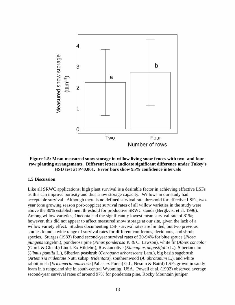
From empirical snow storage measurements, we observed that all willow LSFs were trapping snow throughout the snow accumulation season and that four-row planting arrangements tended to catch more snow than two-row planting arrangements (Table 1.5, Figure 1.5). Across observation dates, willow variety did not have a significant effect in predicting snow transport, but the effect of planting arrangement was significant (P<0.001). On average, four-row planting arrangements tended to capture 1.2 times the snow transport compared to two-row planting arrangements (Figure 1.5).

Table 1.5: Mean snow storage measurements in willow snow fences by number of rows and month during 2014-2015 winter

Number of rows

November January March t m-1

Two 0.98 3.24 2.48 Four 0.93 3.97 3.25

13

a

b

0

1

2

3

4

Two FourNumber of rows

Mea

sure

d sn

ow s

tora

ge(tm

1)

Figure 1.5: Mean measured snow storage in willow living snow fences with two- and four-row planting arrangements. Different letters indicate significant difference under Tukey’s

HSD test at P<0.001. Error bars show 95% confidence intervals

1.5 Discussion

Like all SRWC applications, high plant survival is a desirable factor in achieving effective LSFs as this can improve porosity and thus snow storage capacity. Willows in our study had acceptable survival. Although there is no defined survival rate threshold for effective LSFs, two-year (one growing season post-coppice) survival rates of all willow varieties in the study were above the 80% establishment threshold for productive SRWC stands (Bergkvist et al. 1996). Among willow varieties, Oneonta had the significantly lowest mean survival rate of 81%; however, this did not appear to affect measured snow storage at our site, given the lack of a willow variety effect. Studies documenting LSF survival rates are limited, but two previous studies found a wide range of survival rates for different coniferous, deciduous, and shrub species. Sturges (1983) found second-year survival rates of 20-94% for blue spruce (Picea pungens Engelm.), ponderosa pine (Pinus ponderosa P. & C. Lawson), white fir (Abies concolor (Gord. & Glend.) Lindl. Ex Hildebr.), Russian olive (Elaeagnus angustifolia L.), Siberian elm (Ulmus pumila L.), Siberian peashrub (Caragana arborescens Lam.), big basin sagebrush (Artemisia tridentate Nutt. subsp. tridentata), southernwood (A. abrotanum L.), and white rabbitbrush (Ericameria nauseosa (Pallas ex Pursh) G.L. Nesom & Baird) LSFs grown in sandy loam in a rangeland site in south-central Wyoming, USA. Powell et al. (1992) observed average second-year survival rates of around 97% for ponderosa pine, Rocky Mountain juniper

14

(Juniperus scopulorum Sarg.), and Siberian peashrub LSFs in southeastern Wyoming, with similar soil and climatic conditions as those reported in Sturges (1983). While no studies to our knowledge have documented shrub-willow survival in LSF plantings, Gamble et al. (2014) found 96% post-coppice survival rates for S. purpurea ‘Fish Creek’ grown in hedgerows in alley cropping systems at two sites in southern Minnesota.

The performance and survival of shrub-willows in our study was likely influenced by the lack of pre-emergent weed control the year before planting, a best management practice identified for willow plantings (Abrahamson et al. 2010) and LSFs (Gullickson et al. 1999). This resulted in many competing annual and perennial weeds in the study area during the first and second growing seasons. Despite post-emergent herbicide applications, a total of 32.5 hours were spent hand-weeding the study site during the first two years of establishment. If established without best management practices, this high degree of maintenance is a primary drawback for shrub-willow LSFs (Heavey 2013). As a pioneer species, willows require full sunlight and intensive weed control for optimal survival and growth during the first few years of establishment (Kuzovkina and Quigley 2005; Abrahamson et al. 2010; Heavey 2013). Therefore, while willow survival in the study LSF was adequate two years after planting, proper pre-emergent weed control the year before planting may have improved survival rates and reduced the need for manual weed removal.

In addition to survival, the height of a snow fence also influences the snow storage capacity of a LSF, as height is proportional to a snowdrift’s cross-sectional area (Tabler 2003). The average height in our willow LSF treatments was approximately 1 m after one growing season post-coppice. This is lower than heights observed for two-year-old (one growing season post-coppice) willow LSFs in New York State, where the mean height for varieties S. miyabeana ‘SX64’ and S. purpurea ‘Fish Creek’ was 1.9 m (Heavey 2013; Heavey and Volk 2014). While this difference may be due to a number of factors, such as different soil and climatic conditions or variety selection, this could also be a result of insufficient pre-emergent weed control at our site, as Heavey and Volk (2014) selected LSFs that were established with best management practices. Another factor that may have influenced willow growth at our site is the tendency for right-of-way soils to be compacted as result of road construction. While we did not assess soil properties related to this in the current study, Souch et al. (2004) noted a 12% reduction in stem biomass of S. viminalis under heavily compacted sandy loam relative to a control, but found the effect of moderate compaction to be insignificant on willow growth in clay loam and sandy loam. Although willows are generally known to tolerate harsh soil conditions (Kuzovkina and Volk 2009), future willow LSF studies should investigate soil physical properties, such as bulk density and porosity, as they relate to establishment. Nevertheless, willows at our site had comparable heights to coniferous and deciduous LSF species after eight growing seasons in Wyoming (Powell et al. 1992), and were taller than most LSF species after five growing seasons in separate study in Wyoming (Sturges 1983). While trees and shrubs in Wyoming likely experienced harsher growing conditions than in our study, willows in our study tended to have faster growth rates, which Heavey and Volk (2014) also noted when comparing LSF shrub-willow growth rates to species traditionally used in LSFs.

When comparing heights among willows and rows in the snow fences, we observed an edge effect between the outer and inner rows, with outer rows tending to be shorter than inner rows.

15

Interestingly, the converse trend was found by Gamble et al. (2014) during the establishment of multi-row poplar hedges in alley cropping systems, wherein edge trees tended to be larger than center trees. Moreover, this trend was only observed for north-south hedges and not east-west hedges (Gamble et al. 2014), which was the orientation of our LSFs. Other than Gamble et al. (2014), little information exists on differences among row establishment in windbreaks. Differences in wind stress were likely negligible between exposed outer rows and inner rows, as outer rows were observed to be relatively porous during the first growing season and thus likely offered little wind protection for inner rows. Furthermore, Sturges (1983) found no differences between the establishment of LSFs with and without the wind protection of an upwind structural snow fence. It is possible that weeds adjacent to the plot boundaries competed with outer rows for light, nutrients or moisture, as these areas were not cultivated. Herbicide drift from adjacent fields and rights-of-way or soil compaction from machinery could have also stunted outer rows. Ultimately, more research is needed to explain the cause of these edge effects.

As with snow fence height, porosity is a structural variable that determines the geometry of snow drifts around a fence (Tabler 2003). Measured porosity at our study was high overall, with an average of 83%. As expected, porosity was lower in four-row arrangements than in two-row arrangements. The average porosity for two-row arrangements in our study (87%) agreed with the average 88% porosity found for two-year-old (one growing season post-coppice), two-row willow snow fences in New York State (Heavey and Volk 2014). That porosity did not differ significantly among willow varieties corroborates Kuzovkina and Volk (2009) and Isebrands et al. (2014) who suggested that many willow varieties share morphological characteristics suitable for LSFs, such as relatively consistent porosity along the height of the plant.

The height and porosity of a LSF can be used to predict its snow storage capacity (Qc), which can then be compared to the mean annual transport (Q) for the LSF’s location to determine its overall functionality (Tabler 2003; Heavey and Volk 2014). At our study location, we found a Q of 39.9 t m-1, classified as “light to moderate” snow transport (Tabler 2003), over a snow accumulation season (SAS) of Nov 16 to Mar 17. These values agree with a range of Q and SAS dates found across southern Minnesota (Shulski and Seeley 2001; 2004). Values of Qc in our study ranged from <1–9 t m-1, which were comparable to those found for one- and two-year-old shrub-willow LSF in New York State (Heavey and Volk 2014). By comparing Qc to Q, we found that none of our willow LSFs, regardless of variety and planting arrangement, were able to match or exceed Q at the study site after two growing seasons. At most, four rows of S. purpurea ‘Fish Creek’ could potentially trap 24% of Q at our location. That none of the Qc values were equal to or greater than Q after one growing season post-coppice is consistent with the findings of Heavey and Volk (2014). They found that Qc values for shrub-willow LSFs were unable to exceed local transport conditions until three years after planting. It is important to note that in all sample locations in Heavey and Volk (2014), Q was classified as “light” to “very light” (Tabler 2003) with none of the estimated Q values exceeding 20 t m-1. In Minnesota, however, wind-defined snow transport conditions tend to be heavier than those reported by Heavey and Volk (2014), especially in western and southern Minnesota (Shulski and Seeley 2004). As such, LSFs in western and southern Minnesota may require additional years of growth before they are able to exceed Q values.

16

By applying models developed by Heavey and Volk (2014) relating two-row willow LSF age to height and porosity, we found that two-row willow LSFs could exceed the Q for south-central, Minnesota after four growing seasons (three growing seasons post-coppice) by approximately 113%. Incorporating our relationship between number of rows and porosity, we found that the Qc of four-row arrangements could exceed Q after three growing seasons (two growing seasons post-coppice) by approximately 35% and by 149% after four growing seasons. The probability of annual snow transport exceeding Q by 100% is less than 0.1% (Tabler 2003; Heavey and Volk 2014); thus, predicted Qc values for both two- and four-row planting arrangements could potentially exceed a twofold increase in Q after three growing seasons post-coppice. While these estimates may be useful in projecting future Qc values, they are based on willow growth in New York State, which likely has some differences in growth conditions. Additionally, willows LSFs used by Heavey and Volk (2014) to develop the height and porosity regressions were not harvested, so these estimates may not be applicable to willows harvested on a short rotation. Therefore, future research should document willow LSF growth and porosity to evaluate the model estimates.

We observed throughout the winter of 2014-2015 that all willow plots were trapping snow, and that four rows tended to catch more snow than two rows. However, we were not able to compare our measurements to the modeled Qc results. The models developed by Tabler (2003) assume there are few days with above-freezing temperatures between the onset and end of the SAS. With this assumption, measurements taken at the end of the SAS should provide the total amount of snow trapped by a LSF during the SAS (e.g., Shulski and Seeley 2001). In our case, we had many dates during the 2014-2015 SAS in which temperatures were above freezing, as well as rain events. This prevented us from obtaining total SAS measurements, but did allow for comparison among willow varieties and planting arrangements. These measurements confirmed our expectation that LSFs with four rows capture more snow than LSFs with two rows, likely due to the generally lower porosity in four rows. Willow variety ultimately had no effect on observed snow storage capacity, which may be explained by the lack of a variety effect on porosity. These observations suggest that, for early snow storage capacity, four rows of willows are more effective than two rows. Additionally, since willow variety had no effect on snow capture, multiple varieties may be appropriate in a LSF, which could improve a LSF’s resiliency to disease, pest outbreaks or other disturbances (McCracken et al. 2001; Mundt 2002). Furthermore, this could allow varieties to be selected for LSFs based on site-specific factors. Ultimately, these implications should be evaluated in future studies.

1.6 Conclusion

In comparing the effectiveness of willow LSFs with three different willow varieties and two different planting arrangements, we found all planting designs to have adequate survival and growth after one growing season post-coppice. However, establishment could likely be improved with proper weed control practices. Furthermore, care should be taken to prevent herbicide drift around LSFs as we did observe dieback and lower growth on edge rows. Although this could not be attributed specifically to herbicide drift, preventing herbicide drift is a best management practice during LSF establishment (Shaw 1988) and may have improved edge-row establishment in our study.

17

Porosity of willow LSFs after one growing season post-coppice was high across all treatments, but on average lower in four-row planting arrangements than two-row arrangements. Using models by Tabler (2003), measured height and porosity for willow LSF treatments translated to low overall snow storage capacity (Qc) values relative to the mean annual snow transport (Q). Using models from Heavey and Volk (2014), however, we found that willow LSFs could exceed Q in three to four growing seasons after planting. Although we were unable to evaluate model predictions with field measurements, field measurements revealed that all willow LSFs were trapping snow throughout the 2014-2015 winter and that four-row planting arrangements trapped more snow than two-row arrangements, as expected. Willow variety did not have an effect on measured snow transport, suggesting that multiple shrub-willow varieties could be used in LSFs based on site-specific factors. Ultimately, these finding should be evaluated in future years and studies, especially during winters with consistently below-freezing temperatures. Overall, these results add to the literature that shrub-willows may be an appropriate choice for LSFs (Heavey and Volk 2014, Kuzovkina and Volk 2009).

18

THE ECONOMICS OF PLANTING AND PRODUCING BIOMASS FROM WILLOW (SALIX SPP.) LIVING SNOW FENCES

2.1 Abstract

Blowing snow adversely affects winter transportation conditions by reducing driver’s visibility, creating icy roads, and/or depositing snow drifts in the travel lane. Blowing snow problems are prevalent in snowy and windy climates and in landscapes that lack sufficient vegetation to trap snow. Maintaining safe roads with blowing snow problems can be a costly challenge for transportation agencies. Living snow fences (LSFs) are semi-permanent living structures that can reduce blowing and drifting snow and offer environmental benefits (e.g. carbon sequestration, wildlife habitat). Recently, willows (Salix spp.) have been evaluated as a potential LSF due to the relative ease of planting, ability to establish well, grow fast, and reduce the cost of plant material. To evaluate the potential of willow LSFs, this study analyzes the costs of planting and establishing a willow snow fence and the viability of harvesting biomass. This study found that the costs of planting and establishing a willow LSF is $10.10 m-1 of double rows plus a fixed cost of $1,784 per willow LSF. Biomass harvest is prohibitively expensive for the typical willow LSF due to the small scale of production. However, corridor length willow LSFs, in which planting and establishment costs are defrayed due to the transportation benefits, can produce biomass at a cost of $26 dry-Mg-1.

2.2 Introduction

Blowing snow adversely affects winter transportation conditions by reducing driver’s visibility, creating icy roads, and/or depositing snow drifts in the travel lane. Maintaining safe roads with blowing snow can be a costly challenge for transportation agencies. Blowing snow problems are prevalent in snowy and windy climates (Shulski and Seeley 2001, 2004) and in landscapes that lack sufficient vegetation to trap snow (e.g. agricultural regions dominated by annual crops). Living snow fences—a windbreak agroforestry practice—reduce blowing snow by trapping snow before it reaches the roadway (Tabler 1980, 1997, 2003). The reduction in the costs of snow and ice removal and the benefits of increased mobility and a reduction in snow and ice related crashes over the life of the snow fence can exceed the cost of the snow fences. Installing and establishing snow fences is a good investment of public money.

Options for snow fences include structural material (e.g. wood slats or rigid plastic) or plants (e.g. shrubs or corn stalks). Living snow fences (LSFs) are semi-permanent living structures that offer environmental benefits (e.g. carbon sequestration, wildlife habitat) in addition to reductions in blowing snow. The effectiveness of well-established LSFs to trap blowing snow is well documented (Shaw 1988; Powell et al. 1991; Heavey 2013; Heavey and Volk 2014). In addition, the economic performance of LSFs can be better than structural snow fences (Daigneault and Betters 2000; Wyatt et al. 2012). Traditionally, shrubs such as dogwood have dominated LSFs plantings. Recently, willows (Salix spp.) have been evaluated as a potential LSF due to the relative ease of planting, ability to establish well, grow fast, and reduce the cost of plant material (see Chapter 1). However, there is limited information on the actual installation and establishment costs of willow for living snow fences.

19

The first half of this paper calculates the cost of installation and establishment of a willow LSF by documenting the actual costs of a willow LSF planting in Waseca, Minnesota. The willow LSF had two planting layouts/arrangements (i.e., two and four rows). Based on the fixed and variable (i.e., rows and length) costs, this paper offers a model for estimating willow LSF installation and establishment costs based on the number of rows and the length.

Willow LSFs also offer the opportunity to produce biomass (Abrahamson et al. 2010; Zamora et al. 2014; Amichev et al. 2015). Our willow snow fence planting evaluated three cultivars that were specifically developed for biomass production. Willow is a candidate feedstock for bioenergy production because of its high yield potential. The costs of planting, harvesting, and transporting willows in fields is well documented (Rosenqvist and Dawson 2005; Styles et al. 2008; Buchholz and Volk 2010). However, these costs do not exist for willows established as LSFs. The most notable difference between biomass production in willow LSF and other willow biomass production systems is that willow LSF can be multi-output (i.e., biomass and snow storage) production systems. Payments for snow storage can defray the planting and establishment cost of willows for biomass, decreasing some of the costs of production. In addition, the linear nature of a snow fence would reduce harvester turn time. However, the small scale of production from typical willow snow fences could dramatically increase unit costs.

The second half of this paper estimates the biomass production costs for the willow snow fence planting in Waseca, Minnesota, USA using planting design described in Chapter 1. Furthermore, this paper also estimates the biomass production costs for a longer corridor-length living snow fence to emphasize the importance of economies of scale in producing low cost biomass.

2.3 Methods

2.3.1 Planting and Establishment

The willow LSF was established in May 2013 on the Minnesota Department of Transportation (MnDOT) right-of-way on the north side of U.S. Highway 14 (44o03’32” N; 93o31’12”) in Waseca, Minnesota, near the University of Minnesota’s Southern Research and Outreach Center (SROC). The 454 m willow LSF was planted to alleviate a blowing snow problem downwind (i.e., south) of the site and as part of a field experiment to evaluate snow capture potential of hybrid willow using two planting arrangements (two and four rows) and three cultivars (Salix purpurea ‘Fish Creek’, S. purpurea × S. miyabeana ‘Oneonta’, and S. caprea × S. cinerea ‘S365’) (see Chapter 1 for details about the experiment). Detailed data was also collected on the quantity of inputs such as labor, materials, and machinery. The research team ensured to separate the inputs needed to successfully plant and establish the willow LSF from the inputs that were only research related (e.g., labor for growth measurements). This was done so that the inputs best represented those needed to plant and establish a willow LSF. In most cases, the prices of the inputs in the research project were not used. Instead, the prices were obtained from the literature and suppliers.

20

2.3.2 Labor

The labor costs in this section include only non-machinery labor. Machinery labor is included in the machinery costs. Labor hours for four non-machinery activities where collected: demarcating the planting area with flags, installing erosion control, planting, and coppicing (Table 2.1). Demarcating the planting area was the only activity that required a skilled worker. Installation of erosion control, planting, and coppicing did not require a worker trained in a specific skill1. Hand weeding was separated out of the analysis because if time permitted2 to use best management practices3 (e.g., proper site preparation the year before planting), there would have been no need to hand weed the willow LSF. Hand weeding was employed to minimize weed competition for the experiment. Weed competition without weeding would likely reduce growth, which could impact willow LSF’s functionality.4

Table 2.1: Labor usage and costs for farm workers in Waseca, Minnesota during the willow living snow fence establishment

Hours Skilled Total Demarcating planting area with flags 18 1a $486 Erosion Control 31.5 0 $595 Planting 28.5 0 $539 Coppice 10 0 $189

Subtotal 88 $1,809 Hand Weeding 32.5 0 $471

Total 120.5 $2,279 a “1” signifies “skilled” whereas “0” signifies “unskilled”

The labor costs were estimated using two different labor rates and a fringe rate of 35% based on Buchholz et. al. (2014). The rates were the farm worker rate for skilled ($20 hour-1) and unskilled ($14 hour-1) workers (Buchholz et al. 2014) and match closely with rates ($20 and $15) for enterprise budgets in Minnesota (Lazarus 2015a). With fringe benefits, these rates are $27 and $18.90/hour.

The total cost of labor with hand weeding was $2,279. Administration and design costs were not included in the labor cost as they were difficult to separate from the research costs. In our experiment, the actual labor cost was likely higher than the estimated labor costs. For instance, the use of wattle was necessary for this particular willow snow fence because of the high erosion potential of the project sites, which is not the case on all sites.

1 Teenagers from local non-profits groups were utilized and compensated for many of the activities. 2 Grant funding was not awarded to allow work to begin prior to the Spring 2013 3 Best management practices for willow planting recommend a glyphosate application in the fall proceeding the spring

planting. 4 Weed competition is most problematic in the planting year. Willow competes well with weed once established.

21

2.3.3 Chemicals

Installation and establishment of the willow LSF included three chemical applications. In spring 2013, before planting and tillage, Roundup Weather Max [glyphosate, N-(phosphonomethyl) glycine] was applied to control pre-emergent weeds. Shortly after planting Transline [a.i. clopyralid (3,6-dichloro-2-pyridinecarboxylic acid)] and Poast {a.i. sethoxydim 2-[1-(ethoxyimino)butyl]-5-[2-(ethylthio)propyl]-3-hydroxyl-2-cyclohexen-1-one} were applied to control post-emergent weeds. In the following spring of 2014, a second post-emergent application of Transline was applied to reduce weed competition (Table 2.2). Prices for the chemicals are based on the Minnesota Enterprise Budget (Lazarus 2015a).

Table 2.2: Chemical usage, rates, and prices for Willow living snow fence establishment in Waseca, Minnesota

Chemical Applications (#) Rate (L ha-1) Price (L-1) Cost (ha-1) Roundup Weather Max

1 2.34 $16.64 $38.92

Transline 2 0.78 $121.52 $189.45 Poast 1 1.39 $21.13 $29.34

Total $257.71

2.3.4 Machinery

Many different types of non-harvest machinery were used during the installation and establishment of the willow LSF (Table 2.3). During chemical applications5, a tractor and chemical sprayer were used taking 1.5 hours to complete. Before disturbing the soil, erosion control was installed using skid steer to transport the wattles. In June 2013, one week before planting, the site was rototilled. For our analysis, a moldboard plow was substituted for the rototiller because cost data of a rototiller was not available. Furthermore, the planter was used not to plant the willow cuttings but to mark the rows. Overall, a total of 6.5 hours of tractor usage were estimated for the study. The total cost was based on a 130 horsepower mid-engine front-wheel-drive tractor. Coppicing required the use of a brush trimmer. We included the total cost of the brush trimmer in the analysis as no information on the maintenance, repair, and depreciation for trimmers exists. The machinery cost data was taken from Lazarus (2015b) and Plastina et al. (2015).

5 Details of the application timing can be found in the chemicals section.

22

Table 2.3: Non-Harvest machinery, costs and hours for willow living snow fence establishment in Waseca, Minnesota

Machinery Cost Hours Total Cost Chemical Spray $63.80a per hour 4.5 $287.10 Skid Steer $53.40a per hour 5.25 $280.35 Moldboard Plow $31.47b per hour 1 $31.47 Planter $32.99b per hour 1 $32.99 Tractor $26.25b per hour 6.5 $170.63 Trimmer $329.00c each $329.00

Total $1,131.54 aPlastina et. al. 2015; bLazarus 2015; cInvoice

2.3.5 Planting Stock

Willow cuttings were obtained from Double A. Willow Inc. in Fredonia, New York, USA. The price of each 20-cm cutting was $0.50 plus a $0.15 out of state royalty and a 15% sales tax6 for a total cost of $0.75/cutting. Willow cuttings that did not survive were replaced a month after planting. Due to the different rates of survivability, different designs in the willow snow fence required differing levels of replacement (Table 2.4). The final two rows in the table are the total cuttings, replacement, and cost for all the 2- and 4-row planting arrangements designs. This was used to calculate the average planting stock cost for 2 and 4 rows.

6The price of the willow cuttings is based on the purchase of with the volume discount of 500+ plants and out-of-state

purchasing.

23

Table 2.4: Planting stocks, replacement, and costs by willow variety based on planting arrangement designs

Variety Rows Length # Cuttings # Replacement Total Cost Taxes Total

Fish Creek 2 248 248 5 253 $325.65 $48.85 $374.50

Fish Creek 4 248 496 18 514 $656.50 $98.48 $754.98

Oneonta 2 248 248 17 265 $333.45 $50.02 $383.47

Oneonta 4 248 496 35 531 $667.55 $100.13 $767.68

S365 2 248 248 13 261 $330.85 $49.63 $380.48

S365 4 248 496 10 506 $651.30 $97.70 $749.00

2-Row Total 2 744 744 35 779 $989.95 $148.49 $1,138.44

4-Row Total 4 744 1488 63 1551 $1,975.35 $296.30 $2,271.65

2.3.6 Erosion Control

Additional supplies were used as part of the installation and maintenance. The willow LSF required the use of straw wattles for erosion control. Total cost for all supplies related to the erosion control was $1,819.

2.3.7 Harvest

To calculate harvest costs, we used a modified version of the harvest module in the Eco-Willow 2.0 decision support tool (Buchholz et al. 2014). The Eco-Willow tool is restricted for scenarios with a minimum of 10 ha and harvest cycles of 3 to 4 years. A 2- or 4-row willow snow fence at the site would occupy 0.11 and 0.21 ha, respectively. To calculate harvest costs we used a harvester material capacity of 40 dry Mg per hour based on a minimum of 18.5 wet Mg per ha (Eisenbies et al. 2014). Due to the linear nature of the living snow fence we assumed no loss in efficiency from turning around. All other harvest costs are taken from the Eco-Willow defaults which includes the cost to mobilize the harvester to the site (Table 2.5).

Table 2.5: Harvest and transportation equipment cost of willow living snow fence in Waseca, Minnesota

Rental Rate

(hour-1) Fuel

(L hour-1) Total

(hour-1) Mobilization Harvester $200.00 121 $315.20 $565.50 Tractor and Wagon $50.00 30 $78.80 On-site

Loader $18.75 Included $18.75 On-site

Truck $75.00 Included $75.00 Roundtrip

2.3.8 Transport

Transport costs were calculated using the Eco-Willow 2.0 (Buchholz et al. 2014) at the suggested values. Equipment includes a truck and a loader. The total transportation costs per harvest are the same for the 2- and 4-row willow LSF. This is because the 2- and 4-row willow snow fence yields are less than a truck load.

24

2.4 Results and Discussion

We evaluated three willow LSF scenarios. Two of the scenarios calculate the costs for a willow LSF with the same length (454 meter) as the actual willow LSF that was analyzed for planting and establishment costs. One of these scenarios has 2 rows of willows and the other has 4 rows. These two scenarios represent the typical length of a snow fence that protects a single blowing snow problem. The third scenario that we evaluated was a 4-row willow LSF that is 18.1 km long and has an area of 8.3 hectares. This longer snow fence represents a transportation corridor-length snow fence that has a production acreage near the minimum recommended acreage for cost efficient biomass production (Buchholz et al. 2014).

2.4.1 Planting and Establishment

The actual willow LSF had 2 rows for 50% of the length and 4 rows for the other 50%. Some of the planting and establishment costs will vary by the number of rows and some will not. Erosion control required a single row of straw wattles to be installed along the entire willow snow fence. Thus, this total cost is the same for the 454 meter 2-row and 4-row scenarios. We also included erosion control for the corridor length willow LSF. All of the other planting and establishment costs were calculated on a per double row basis. For these costs, the total and per meter costs for the 4-row 454-meter willow snow fence are twice those of the 2-row willow snow fence (Table 2.6).

The unit costs were multiplied by the length of the snow fence or the total length of the double rows, depending on how the unit costs were calculated. The planting and establishment of a 2-row 454 meter willow LSF is estimated to cost a total of $6,367 or $14.11 per meter (Table 2.6). A 4-row 454-meter snow fence has an estimated total cost of $10,955 or $24.18 per meter. In order to develop a model to predict the cost of a willow LSF based on the number of rows and length we determined the best fit for the 2- and 4-row snow fences costs. We estimated a fixed cost of $1,784 per willow LSF and a variable cost of $10.10 per double row meter. For example, the estimated cost of a 4-row (i.e. 2 double rows) 100-meter willow snow fence is $3,804.7

7 The calculation is $1,784 + 2 × 100 × $10.10.

25

Table 2.6: Summary of per meter and total establishment costs for willow living snow fences in Minnesota, USA

Actual Willow Living Snow Fence Corridora Rows 2 4 4 Meters 454 454 18,117 Hectares 0.10 0.21 8.27

Per Meter

Erosion Control $4.01 $4.01 $4.01 Planting Stock $5.02 $10.02 $4.65 Chemical $0.06 $0.12 $0.10 Machinery $1.66 $3.33 $3.57 Labor $2.66 $5.32 $2.38 Weeding Labor $0.69 $1.38

Total $14.11 $24.18 $14.72

Total Erosion Control $1,819 $1,819 $72,679 Planting Stock $2,277 $4,543 $84,284 Chemical $27 $53 $1,838 Machinery $754 $1,509 $64,645 Labor $1,206 $2,412 $43,189 Weeding Labor $314 $628

Total $6,397 $10,965 $266,635 aThis longer snow fence represents a transportation corridor-length snow fence that has a production acreage near the minimum recommended acreage for cost efficient biomass production (Buchholz et al. 2014)

To calculate the planting and establishment costs of the larger scale corridor project we used the EcoWillow 2.0 tool. The reason for this is that the hand planting and establishment method used in the actual willow snow fence is only cost-effective for small scale projects. The scale of the corridor project is large enough to justify using similar planting equipment as the willow biomass systems. This reduces the per meter planting and establishment costs by 39% from the 454-meter 4-row willow snow fence.

2.4.2 Conservation Program Cost Sharing

Both the Conservation Reserve Program (CRP) and the Environmental Quality Incentive Program (EQIP) offer establishment cost-share for LSFs. LSFs that are to be harvested for biomass are not eligible for cost-share dollars under CRP. EQIP offers establishment cost share. The preparation and establishment cost share is based on the number of acres. The planting cost share is a flat rate based on length and rows. The reimbursement rates for EQIP LSFs is $2.17 per meter per row (Table 2.7).

26

Table 2.7: Reimbursement rates in US Dollars per hectare for two preparation methods and three previous vegetation types

Previous Vegetation Preparation Cropland/Grassland Shrub/Brush Trees Mechanical $47 $336 $2,664 Chemical $54 $128 N/A

Using these reimbursement rates, chemical preparation, and grassland as the previous vegetation rate, Table 2.8 shows the calculated cost share for the 454 m two and four row willow LSFs. The EQIP cost share covers between 31-36% of the establishment.

Table 2.8: EQIP cost share for 2- and 4-row willow living snow fences Row

Feet Acres Site Prep Planting Cost Share Net Cost % Cost Share

2 Row 907 0.10 $5.62 $1,964 $6,397 31% 4 Row 1814 0.21 $11.24 $3,928 $10,965 36%

2.4.3 Comparison to Current Living Snow Fence Costs

One advantage of willow snow fences is the relatively low cost of planting stock, the simple planting procedure, and the high rate of survivability. Typical planting stock for living snow fences is 30 - 60 cm bare root shrubs. In 2014, the average bid price for the Minnesota Department of Transportation (MnDOT) for planting 30 cm bare foot shrubs was $50.50/plant. This includes site preparation, weed control, adding 10 cm of compost to the planting beds, furnishing and installing the plant material, watering, wood chip mulch, and guaranteeing the plant for survival. From 2012 to 2014 the average bid price increased by 23% year-1. In comparison, the planting and establishment cost for the willow LSF in this project is $4.30 and $3.68 per plant for 2 and 4 rows, respectively. It is likely that the estimates of the willow planting in this paper are lower than what a contract price would be to plant willows. The estimates of the willow LSF costs in this paper did not include adding compost and mulching, the cost of insuring the plants, and the overhead. The only way to truly compare the shrub contract price with a willow contract price is to receive bids on willow planting on a willow snow fence project.

2.4.4 Biomass Production

In addition to installation and establishment costs, biomass production from willow LSFs was also estimated. Harvest and transport costs as well as the actual planting and establishment costs of our study were used to estimate biomass production costs (Table 2.9). The first year is the establishment year including the coppicing of the willows.

27

Table 2.9: Summaries of the total, per hectare and per meter costs for biomass production from a 454-meter 2- and 4-row and corridor-length willow living snow fence in Waseca,

Minnesota

Actual Willow Living Snow Fence (454 meters) Corridor

2 Rows 4 Rows 4 Rows

Total Per Hectare Per Meter Total Per Hectare Per Meter Total Per Hectare Per Meter

Transport $262 $2,533 $0.58 $262 $1,268 $0.58 $2,942 $356 $0.16

Harvest $676 $6,538 $1.49 $713 $3,447 $1.57 $4,996 $604 $0.28

Plant $6,397 $61,830 $14.11 $10,965 $52,987 $24.18 $266,635 $32,257 $14.72

2.4.5 Enterprise Budgets

The cost by operation year type is first summarized followed by an analysis of cash flow for a 25-year stand life for 454 m 2-row and 4-row willow LSF planting arrangements and for the longer corridor willow LSF.

The total transportation costs are $262 for the 454-m 2- and 4-row willow LSF (Table 2.9). The transportation costs are the same even though the yield for the 4-row willow snow fence is double that of the 2-row LSF. This is because the 4-row willow LSF yield is less than a truck load.

2.4.6 Cash Flow

The cash flow shows the cost of production over the stand life (Table 2.10). The first year is the planting and establishment. The willow is harvested every 6 years for the 454 m 2-row willow LSF, 4 years for the 454 m 4-row willow LSF and 3 years for the corridor-length willow LSF. In the years that the willow is not harvested the only cost is the land rent. The net present value, 𝑁𝑁𝑁𝑁𝑁𝑁 = ∑𝑇𝑇 𝑉𝑉𝑡𝑡 ( )𝑇𝑇

𝑡𝑡=1 𝑡𝑡−1, and the annualized net present value, 𝐴𝐴𝑁𝑁𝑁𝑁𝑁𝑁 = 𝑟𝑟 1+𝑟𝑟(1+𝑟𝑟) (1+𝑟𝑟)𝑇𝑇 𝑁𝑁𝑁𝑁𝑁𝑁, are

−1calculated for the three scenarios using a 5% real discount rate (𝑟𝑟). The results are presented in Table 2.11.

2.4.7 Costs of Production

Table 2.12 shows the summary of the costs of production of willow biomass using a LSF design. Overall, the total production costs are higher for the 4 rows than the 2 rows due to having twice the area of production. However, production costs for 4 rows per area and per length are lower than 2-row planting arrangements. This is a result of economies of scale. Using the biomass yield averages (4.3 dry-Mg year-1), from other experiments at the same research station, for the cultivars grown in our study we estimated the breakeven price by examining the cost of production on a dry Mg basis. The lowest breakeven price (i.e., cost of production) is $282 per dry Mg for the 4-row corridor-length willow LSF. However, if the biomass is harvested from a willow LSF in which the planting and land costs are defrayed by payments for the snow storage, then the lowest breakeven price is $26 per dry Mg for a 4-row corridor-length willow LSF.

28

Table 2.10: Enterprise budget cash flow for willow living snow fence in 2- and 4-row arrangements.

Year Planting and Establishment Maintenance Harvest 2 Row Land $61 $61 $61 Plant $6,397

Harvest $676 Transport $262

Total $6,458 $61 $999 4 Row Land $121 $121 $121 Plant $10,965 Harvest $713 Transport $262

Total $11,086 $121 $1,097 4 Row Corridor Land $4,851 $4,851 $4,851 Plant $266,635 Harvest $4,996 Transport $2,942 Total $271,487 $4,851 $12,789

Table 2.11: Summary of costs by net present value and annualized net present value for a 25-year stand life using 2- and 4-row planting arrangements and corridor-length willow

living snow fences

Net Present Value Annualized Net Present Value Actual Willow LSF (454

meters) Corridor Actual Willow LSF (454

meters) Corridor

2-row 4-row 2-row 4-row Land $856 $533 $68,374 $61 $121 $4,851 Plant $6,093 $10,443 $253,938 $432 $741 $18,018 Harvest $1,307 $2,522 $20,826 $93 $162 $1,478 Transport $506 $2,032 $12,264 $36 $60 $870

Total $8,762 $15,529 $355,402 $622 $1,084 $25,217

29

Table 2.12: Summary of annualized net present value of the 454-meter 2- and 4-row planting arrangement and the corridor-length willow living snow fences

Actual Willow LSF (454 meters) Corridor 2-row 4-row

Total Per Hectare

Per dry Mg

Total Per Hectare

Per dry Mg

Total Per Hectar

e

Per dry Mg

Planting and Land Costs $493 $4,765 $550 $862 $4,167 $376 $22,869 $2,767 $256 Harvest and Transport $129 $1,243 $143 $222 $1,071 $97 $2,348 $284 $26

Total $622 $6,008 $693 $1,08

4 $5,238 $473 $25,217 $3,051 $282

2.4.8 Biomass facilities in Minnesota

Harvesting biomass from a willow LSF that is of typical size for a landowner, such as the 454-meter LSF analyzed in this paper, is, at this time, unlikely to be profitable. However, if employed on a larger scale, there are over 40 active biomass facilities in Minnesota that utilize woody biomass for energy (Figure 2.1; Appendix C). These have been identified through the Wood2Energy Project (2015) and the Minnesota Department of Natural Resources (DNR 2015; Dirkswager 2015). The Wood2Energy Project is a collaborative effort initiated by the University of Tennessee to report the state-of-the-science of woody biomass to energy conversion processes in North America. As part of this effort, the project has developed and is continually updating an online database of operational biomass utilization and processing facilities throughout the continent. The Minnesota DNR also tracks active woody biomass energy facilities in Minnesota.

Currently, most Minnesota biomass facilities are concentrated in the northern forested region of the state. At this time, most facilities are sourcing biomass from loggers and not landowners (Dirkswager, personal communication, 2015). Facilities generally pay a certain price for an annual supply of a certain amount of wood, at a certain amount of moisture, usually in the form of either clean or dirty chips. Dirty chips with 35-45% moisture are typically sold for around $35 per green ton (0.9 Mg), whereas clean chips with a similar moisture content are sold for around $45 to $50 per green ton. As long as the biomass meets a facility’s specifications (e.g., moisture content, bark kept on or removed, dirty or clean chips, size), facilities tend not to be too specific on the origin of woody biomass (Dirkwager 2015). However, at this time, there is little information on facilities sourcing wood from short-rotation crops, such as willow.

2.5 Conclusions and Implications

The costs of planting and establishing a willow LSF and the viability of biomass harvest were evaluated in this study. The cost to install a 2- and 4-row 454 m willow LSF at the site was estimated at $6,367 and $10,951, respectively. Based on our analysis of a 2-row and 4-row willow LSF, we estimated that the fixed installation and establishment cost is $1,784. The variable cost, the costs that do vary with the size (i.e., double rows and length) is $10.10 per double row meter. A 4 row 100 m snow fence is estimated to cost $7,944. Enrolling this willow LSF into the EQIP conservation program will provide a cost share of 31-36%.

30

Recently, the average per plant bid price from contractors that install and establish LSF for transportation agencies (e.g., MnDOT) has increased by 23% per year. Willows offer an alternative shrub for LSFs that is easier to plant and more cost effective to install. The cost per plant to install the willow LSF ($4.30) was substantially less than the current bid price ($50.50 per plant).

Figure 2.1: Number of active biomass facilities in Minnesota counties

The cost of harvesting and transporting willow biomass is $97 to $143 per dry Mg. This is much higher than other biomass production systems. This is due to the very small scale of production. Breakeven prices are lower for a 4-row corridor-length willow snow fence when compared with the actual 454 m willow LSF. If the costs of planting and establishment are defrayed by payments for snow storage, then the costs of production in a transportation corridor length willow LSF are $26 per Mg.

Willow is an inexpensive shrub that establishes well and is a good candidate as a LSF shrub. Costs of production of biomass from willow LSFs are likely to be prohibitively expensive for the

31

average size LSF even when the planting and establishment costs are defrayed by payments for the snow storage. However, if the willow LSF is going to be planted as a snow control measure and the snow fence protects an entire corridor, then the costs of production could compete with field scale production.

32

ESTABLISHMENT AND GROWTH OF NATIVE AND HYBRID SHRUB-WILLOWS, GRAY DOGWOOD, AND AMERICAN

CRANBERRYBUSH FOR USE IN LIVING SNOW FENCES

3.1 Introduction

As part of evaluating the use of shrub-willows for living snow fences (LSFs), we sought to compare the growth of both hybrid and native willows to two species traditionally used in LSFs in Minnesota, American cranberrybush (Viburnum opulus L. var. americanum Ait.) and gray dogwood (Cornus racemosa Lam.). Both of the traditional LSF species are bushy shrubs with numerous stems that can reach heights up to 5 m (Smith 2008), thereby producing dense, tall barriers for trapping snow in linear plantings. However, the time required for cranberrybush and dogwood shrubs to reach effective LSF heights may be longer than that required for shrub-willows. In the literature, for cultivated and wild populations, American cranberrybush and gray dogwood have reported annual height growth rates of 24-36 cm year-1 (St-Pierre et al. 2005) and 4-20 cm year-1 cm (Boeken and Canham 1995), respectively, although these values only cover a narrow range of biotic and abiotic conditions. For shrub-willows, annual height growth can be as high as 1-3 m year-1, depending on site conditions (Amichev et al. 2015, Gamble et al. 2014). No studies, however, have compared the growth of shrub-willows to traditional LSF species in a similar environment.

Along with evaluating improved (hybrid) shrub-willow varieties, we sought to evaluate establishment and growth of a native willow, slender-leaved willow (Salix petiolaris), to address concerns over promotion of non-native plants in LSFs. With over 450 species worldwide (Argus 1997), willows are adapted to a range of site and climatic conditions and can often provide a local source for a range of environmental applications (Kuzovkina and Quigley 2005). Minnesota has 18 species of native willows growing throughout the state (Smith 2008). Given their distribution and abundance, native willow species may provide a suitable local plant source for LSFs in Minnesota. However, no research has yet been done to assess their potential for LSFs in Minnesota.

Lastly, we sought to evaluate whether coppice timing (e.g., fall or spring) influences establishment and growth in the willows, in order to determine whether it is advisable to leave first-year stem growth over the winter and coppice the following spring, such that first-year stems may serve as a snow barrier. In theory, there should be no difference in growth among coppice dates as long as willows are dormant (Abrahamson et al 2010.), but growth in most willow studies is based on a fall coppice, likely due to easier field access in the fall. This has resulted in little information on growth after a spring coppice.

3.2 Methods

3.2.1 Study site description

The study was located in Waseca, Minnesota, at the University of Minnesota’s Agricultural Ecology Research Farm (44o03’48” N; 93o32’42” W), which is part of the Southern Research and Outreach Center (SROC). Soils at the site are of the Nicollet series (Fine-loamy, mixed, superactive, mesic Aquic Hapludolls) and were formed in loamy, calcareous till and are very

33

deep and well-drained to very poorly drained. The site ranges in slopes between 0 and 5%. Soil characteristics for the study site are presented in (Table 3.1). Prior to establishment, the site was under a drainage study with perennial crops. The site was rototilled in June 2013, approximately one week before planting.

Table 3.1: Selected soil characteristics for shrub establishment at the University of Minnesota’s Agricultural Ecology Research Farm in Waseca, Minnesota

Soil type Soil depth (cm) pH

Electrical conductivity

(μS/cm)

Particulate organic

matter (%) C/N ratio

Clay loam

0-15 5.3 123 2.4 11.00 15-30 5.2 98 2.3 11.28 30-45 5.4 122 2.1 11.25 45-60 5.6 156 2.5 11.20 60-75 5.8 168 2.1 10.28 75-90 5.8 179 1.8 10.06

Values are the average of three composite samples taken for each 15 cm depth increment

3.2.2 Experimental design and planting materials

The study was established in a randomized complete block design in a split plot arrangement with five willow cultivars and two shrub species traditionally used in LSFs in Minnesota (Table 3.2). The study had four replicates with willow cultivars randomly assigned to either a fall or spring coppice treatment, while cranberrybush and dogwood plots were not coppiced, based on standard management practices (Figure 3.1). Hybrid willow cuttings and bare-root plants were obtained from commercial nurseries (Double A Willow Inc., Fredonia, NY, and Shumacher’s Nursery and Berry Farm, Inc., Heron Lake, MN, respectively), while native willow cuttings were collected from dormant plants at the Ottawa Wildlife Management Area near St. Peter, MN. The use of the native willow, S. petiolaris, was recommended by state botanist W. Smith (personal communication) based on its prevalence in the local area.

Table 3.2: Shrub species used in variety/species comparison study Species/hybrid plants Common name USDA Plant

Hardiness Zones Salix purpurea × S. purpureaa Fish Creek 4–6 S. purpurea × S. miyabeanaa Oneonta 4–6

S. caprea × S. cinereaa S365 4–6

S. eriocephala × S. eriocephalaa b S25 4–6 S. petiolarisb Slender-leaved willow NAc Cornus racemosa Lam.b Gray dogwood 3–8 Viburnum opulus L. var. americanum Ait.b American cranberrybush 2–7 a Originated through controlled breeding in New York b Native to Minnesota c NA No available data on hardiness zone, but occurs throughout northeastern United States and much of Canada (Argus 2007)

34

Figure 3.1: Example replicate for the comparison of candidate shrub species for living snow fences. All willows are represented by their common name provided in Table 3.2.

"Native" refers to Salix petiolaris.

The study was established with plots 5.3 m by 5.5 m. Willow plots were planted with 20 cm (8 inch) dormant stem cuttings in a high-density arrangement of three twin rows, following standard willow trial plot guidelines (Cameron et al. 2008). Twin rows were spaced 150 cm apart, single rows 76 cm apart, and plants within a row 60 cm apart for a density of 14,800 willow cuttings ha-1. Dogwood and cranberrybush plots were planted in 5 single rows with 1.2 m between rows and 1.2 m between plants within a row, based on conservation planting guidelines (NRCS 2009), resulting in a density of 6,727 bare-root plants ha-1. Willow plots assigned to a fall coppice were coppiced in December 2013, while those assigned to a spring coppice were coppiced in April 2014.

Shortly after planting, the site was managed for pre-and post-emergent weeds. In 2013, willow plots were sprayed with 0.7 kg ha-1 Transline [a.i. clopyralid (3,6-dichloro-2-pyridinecarboxylic

35

acid)] and 1.3 kg ha-1 Poast {a.i. sethoxydim 2-[1-(ethoxyimino)butyl]-5-[2-(ethylthio)propyl]-3-hydroxy-2-cyclohexen-1-one} to control pre-emergent weeds, while dogwood and cranberrybush plots were treated with 1.3 kg ha-1 a.i. sethoxdim only. In 2014, all plots were sprayed with a mix 0.7 kg ha-1 a.i. clopyralid and 1.3 kg ha-1 a.i. sethoxydin. To control post-emergent weeds, plots were cultivated in July 2013, followed by manual weed control throughout the remainder of the growing season. All plots were assessed for survival approximately one month after planting; plants without any visible growth were replaced with fresh cuttings or bare-root plants to ensure sufficient stocking.

3.2.3 Plant data collection

To evaluate shrub establishment, survival was assessed approximately one month, one growing season (pre-coppice), and two growing seasons (post-coppice) after planting. For the first assessment, all plants were surveyed for visible growth and restocked accordingly. In following assessments, sample plots were used. In willow plots, twelve central plants were assessed in the middle twin row, and 9 central plants were assessed in dogwood and cranberrybush plots.

To assess and compare plant growth, stem counts, diameters and heights were measured in the fall of 2013 and fall of 2014 (pre- and post-coppice, respectively) in the designated sample areas. For all plants in the sample area, the height of the tallest stem was recorded to the nearest centimeter, following standard willow measurements (Cameron et al. 2008). Stem diameters were recorded to the nearest millimeter at 30 cm above the ground for all stems greater than 3 mm, except when only stems less than 3 mm were present.

3.2.4 Statistical analyses

Linear mixed effects models were used to examine the effects of species and year on survival, height, stem count, and stem diameter for all shrubs. For willows only, linear mixed effects models were also used to examine the effects of willow species/cultivar and coppice date on 2014 survival, height, stem count, and stem diameter. For each parameter, species and year (or willow species and coppice date) were included as fixed effects and tested for significance and interaction via Wald’s Chi-square test. To account for the nested structure in both datasets, replicate and plot number were included as random effects (Pinheiro and Bates 2000). Where main effects were significant at α = 0.05, Tukey’s honestly significant difference (HSD) for multiple comparisons was used to test for differences among means at α = 0.05. All statistical analyses were performed in R (v. 3.0.2; R Foundation for Statistical Computing, Vienna, Austria).

3.3 Results

3.3.1 Growth variables by species and year

We found significant main effect of species (P < 0.001) and year (P = 0.02) on shrub survival, without an interaction (Table 3). On average, survival decreased from 92% in 2013 to 88% in 2014 (P = 0.023). By 2014, survival among species and cultivars was not statistically different at P = 0.05, although Fish Creek had the overall highest survival.

36

We found a significant interaction between species and year (P<0.001) on shrub heights. In 2013, willow cultivars/species Fish Creek and Oneonta were among the tallest species, while willow cultivar S25 was more similar to the shorter heights of cranberrybush and dogwood (Table 3.3). From 2013 to 2014, the heights of all willows significantly increased, while the height of cranberrybush and dogwood did not increase significantly. In 2014, all willows were significantly taller than traditional snow fence shrubs, with Oneonta, S. petiolaris and Fish Creek having the tallest heights.

As with height, shrub stem counts and diameters were influenced by the interaction of species and year at P<0.001. From 2013 to 2014, all willows significantly increased in their number of stems and stem diameters, while there was no significant change in cranberrybush or dogwood stem counts or diameters. Willows also had more stems and larger diameters than dogwood and cranberrybush shrubs in 2014.

3.3.2 Effects of coppice timing on 2014 willow growth variables

We did not observe any effect of species or coppice date on willow survival. The interaction of species and coppice date did, however, influence height (P = 0.013) and the number of stems per plant (P < 0.001) (Table 3.4). For plant height, coppice time only had a significant effect on Fish Creek, for which plants coppiced in fall 2013 were taller than plants coppiced in spring 2014. Regarding the number of stems per plant, coppice time significantly affected Fish Creek, for which there were more stems under a fall coppice, and S25, for which there were more stems under a spring coppice. Mean stem diameter was not significantly influenced by coppice date, resulting in the same observations provided in Table 3.3.

Table 3.3: Mean survival, heights, stem counts, and stem diameters for shrub-willows and traditional living snow fence shrubs in 2013 and 2014.

Species/ cultivar Plant type Survival (%) Height (cm) Stem count plant-1 Diameter (mm)

2013 2014 2013 2014 2013 2014 2013 2014 Fish Creek

Shrub-willow

100.0 a 100.0 a 75.0 a,r 175.2 a,s 1.8 a,r 7.8 a,s 3.8 a,r 5.7 a,s Oneonta 85.4 ab 84.4 a 72.3 ab,r 201.4 a,s 2.2 a,r 10.5 b,s 3.9 a,r 7.0 ab,s S365 82.3 ab 81.3 a 56.3 abc,r 127.7 b,s 1.8 a,r 8.1 a,s 4.2 a,r 6.6 ab,s S25 84.4 ab 77.1 a 40.5 bc,r 118.3 b,s 1.2 a,r 6.1 a,s 3.7 a,r 6.1 ab,s S. petiolaris 93.8 a 87.5 a 52.0 abc,r 176.0 a,s 1.6 a,r 6.1 a,s 3.5 a,r 7.2 b,s Cranberry Traditional

snow fence shrubs

100.0 ac 94.4 a 34.5 c,r 34.7 c,r 1.1 a,r 1.6 c,r 3.3 ab,r 3.2 c,r Dogwood 100.0 ac 94.4 a 37.0 c,r 43.2 c,r 1.0 a,r 0.8 c,r 2.3 b,r 1.9 d,r

Means with overlapping letters are not statistically different under Tukey’s HSD at p≤0.05. Letters a-c denote differences among species, while letters r-s denote differences between years. Differences between years are only noted where there is a significant interaction between species and years.

37

Table 3.4: The effect of coppice time and species on 2014 mean willow height and number of stems per plant.

Species/cultivar Height (cm) Stem count plant-1 Fall Spring Fall Spring

Fish Creek 203.3 a,r 147.1 bc,s 11.5 a,r 4.2 b,s Oneonta 194.1 a,r 207.9 a,r 10.8 a,r 10.2 a,r S365 126.1 b,r 129.3 c,r 8.1 ab,r 8.1 a,r S25 96.9 b,r 136.6 c,r 4.5 b,r 7.5 a,s S. petiolaris 181.7 a,r 170.1 abc,r 6.9 ab,r 5.2 a,r Means with overlapping letters are not statistically different under Tukey’s HSD at p≤0.05. Letters a-c denote differences among species, while letters r-s denote differences between years.

3.4 Discussion

Shrub establishment was generally good among species, although little increase in growth occurred in cranberrybush and dogwood shrubs after the first growing season. We observed high overall survival rates among shrubs after the first growing season, but saw an overall decrease in survival after the 2014 growing season. For willows, a slight decrease in survival is not uncommon after coppicing (e.g., Zamora 2014). For cranberrybush and dogwood shrubs, it is possible they were affected by herbicide application in the second year, as they were noted as being wilted at the start of the 2014 growing season, shortly after herbicide application (Figure 3.2). In the first year, at the start of the growing season, cranberrybush and dogwood plots received only a Poast herbicide treatment, but in the second year they received both a Poast and Transline treatment. It is possible that Transline stunted cranberrybush and dogwood shrubs. Transline has the same active ingredient (clopyralid) as Stinger herbicide, which is not registered for use on either dogwood or cranberrybush shrubs (Gullickson et al. 1999).

Other factors that may have influenced survival were the occurrence of droughts during both growing seasons, as well as the presence of competing vegetation. Willows are especially water-limited (Thelemann et al. 2010), and drought can significantly decrease willow survival (Zamora et al. 2014). Additionally, due to the lack of pre-emergent herbicide application the year prior to establishment, as recommended for willow plantings (Abrahamson et al. 2010), shrubs experienced competition among annual and perennial weeds, which is the most common cause of willow failure in the first two growing seasons. Nevertheless, at the end of 2014, all shrubs except for S25 had survival rates above the 80% threshold recommended for productive SRWC stands Bergkvist et al. (1996).

After the second growing season, willows exhibited significantly higher growth characteristics than cranberrybush and dogwood shrubs, with a mean height 4 times greater than that of the traditional LSF shrubs. This is to be expected, as it is not uncommon for shrub-willows to grow 1-3 m during a growing season (Amichev et al. 2015, Gamble et al. 2014), while cranberrybush and dogwood shrubs tend to have lower growth rates. Interestingly, however, neither cranberrybush nor dogwood shrubs increased in growth with regard to height, number of stems, and stem diameter from 2013 to 2014. This again is likely explained by the Transline herbicide

38

application in 2014. Willows, however, had no observable response to the herbicide applications.

Figure 3.2: American cranberrybush with wilted leaves and stems in June, 2014, shortly after herbicide application

Within willows, second-year growth characteristics of the cultivars agreed well with Amichev et al. (2015), who assessed early growth in the same cultivars, among others. Regarding the native willow, little information exists on its growth characteristics in a cultivated setting. In wild populations in Minnesota, S. petiolaris can reach heights of 4 m and basal diameters of 4 cm (Smith 2008). In this study, we found the growth of S. petiolaris was comparable to willow cultivars with the highest growth. This in some ways contrasts to findings of Zamora et al. (2014), who found native willows different than ours to be generally less productive than hybrid willows in central Minnesota. However, given that S. petiolaris is perhaps the most common and abundant willow in Minnesota (Smith 2008) and was collected from a local source and thus well-adapted to local conditions, it is somewhat unsurprising that it was comparable to genetically improved willows in this study.

All willows significantly increased in the number of stems per plant after coppicing, which is typically observed throughout willow production trials. Regarding coppice date, few differences were observed between the fall 2013 coppice and spring 2014 coppice. Fish Creek, however, had significantly lower height and stem counts under the spring 2014 coppice, whereas the converse was true regarding stem counts in S25. It is possible that Fish Creek may be active earlier in the growing season than other willows, and therefore already allocated some its

39

resources to growth at the time of coppice. This has yet to be tested, however, and no new willow leaves were observed at the time of the spring coppice, although some buds were present. That S25 had significantly more stems per plant under the spring coppice than under the fall coppice is interesting and not explained in the literature. Ultimately more research is needed to explain this observation and determine if it occurs at other sites. Other than Fish Creek and S25, coppice date had little effect on willow growth, which agrees with the literature. According to Abrahamson et al. (2010), for example, coppicing can occur anytime between two weeks after leaf senescence and bud swelling in the spring.

3.5 Conclusion

Our goal in this study was to compare establishment and growth characteristics of shrub-willow LSF candidate species/varieties to shrub species traditionally used in LSFs. Additionally, we sought to evaluate whether coppice timing influences establishment and growth in shrub-willows, in order to determine whether it is advisable to leave first-year stem growth over the winter and coppice the following spring, such that first-year stems may serve as a snow barrier. According to literature, there should be no difference in growth among coppice dates (Abrahamson et al 2010.), but growth in most willow studies is based on a fall coppice, likely due to easier field access in the fall, resulting in little information on spring coppice growth.

We found that all shrubs had good establishment, and that all willows outperformed the traditional LSF species. However, due to concerns about herbicide effects on the traditional LSF shrubs, it is difficult to conclude with certainty that willows did indeed outperform the other shrubs. Nevertheless, shrub-willows generally possess higher growth rates than cranberrybush or dogwood shrubs (e.g., Boeken and Canham 1995; St-Pierre et al. 2005).

Within willows, we found that the native willow, S. petiolaris, was comparable in growth to the highest performing cultivars Fish Creek and Oneonta. Given its wide range throughout Minnesota (Smith 2008), S. petiolaris may thus be suitable for living snow fence applications, although it should ultimately be tested in an LSF configuration before widespread adoption. Minnesota has 18 species of native willows throughout the state (Smith 2008); if they can provide effective LSFs, they may provide a local and affordable plant source for plantings around Minnesota.

Most willows showed no difference in response to coppice dates, but the two that did (Fish Creek and S25) showed opposite responses. Ultimately more research is needed to explain this, but a spring coppice date may be suitable for most willow LSF candidates. If a spring coppice is to be performed, it may be useful to coppice earlier than in our study, which was April 9, 2014. Despite the extended winter, we noticed some willow stems were budding already, meaning they had already allocated some of their annual carbon to growth prior to coppice. In an average year, a coppice in early March may be better (Abrahamson et al. 2010).

40

CONCLUSIONS

4.1 Chapter 1

• Shrub willows are very easy to plant with dormant 8-inch cuttings. It took approximately three hours to plant the living snow fence (LSF) experiment with eight people planting and three people coordinating. The LSF experiment planting was approximately 0.25 miles (400 m) and was planted with 2,232 willow cuttings.

• Shrub willows showed overall good establishment and growth. Average heights after two growing seasons (one growing season post-coppice) were around 3.3 feet (1 m). Weed competition and possible soil compaction may have influenced survival.

• It may be useful to apply a pre-emergent herbicide the year prior to planting or another form of weed control, such as landscape fabric. These are best management practices for LSFs and can reduce the need for hand-weeding.

• Ripping the subsoil before planting a willow LSF site may help reduce soil compaction or remove any soil hardpans.

• After two growing seasons (one growing season post-coppice), willow LSFs had potential snow storage capacities ranging from one to nine metric tons per linear meter (t m-1) of snow fence, as evaluated by Tabler’s (2003) models.

• The modeled snow storage capacity was below the predicted mean annual snow transport (40 t m-1) for the study site. Based on these models, willows after two growing seasons were theoretically unable to trap all of the mean blowing snow at the study site.

• Based on willow LSF models developed by Heavey and Volk (2014), willow LSFs at the study site may reach snow storage capacities that exceed the mean annual snow transport after three to four growing seasons (after planting).

• Based on measured snow drift observations, willow LSFs caught an average of 2- 3 t m-1 of snow during the 2014-15 winter.

• We were unable to compare measured snow data to modeled snow data as the models assume there are few thawing or rain events during the winter. In our case, we had many thawing and rain events during the 2014-15 winter.

• Based on measured snow drift observations, willow varieties did not differ in their ability to trap snow. This suggests that incorporating multiple varieties with similar morphology and site requirements can be incorporated into an LSF. This may be advantageous for increasing a LSF’s resilience to insect or disease outbreaks, or other disturbances.

• Four-row LSF arrangements caught more snow than two-row LSFs. Planting four-row LSFs may therefore provide more blowing snow capture earlier than two-row LSFs.

• Shrub willows are a fast-growing and effective plant for LSFs.

4.2 Chapter 2

• The cost to install a two- and four-row 454 m willow LSF at the site was estimated at $6,367 and $10,951, respectively.

• Based on our analysis of a two-row and four-row willow LSF, we estimated the fixed installation and establishment cost at $1,784.

• The variable cost, costs that do vary with the size (i.e., double rows and length), is $10.10 per double row meter. A four-row 100-meter snow fence is estimated to cost $7,944.

41

• Enrolling this willow LSF into the EQIP conservation program will provide a cost share of 31-36%.

• Recently, the average per plant bid price from contractors that install and establish LSF for transportation agencies (e.g., MnDOT) has increased by 23% per year.

• Willows offer an alternative shrub for LSFs that are easier to plant and more cost effective to install. The cost per plant to install the willow LSF ($4.30) was substantially less than the current bid price ($50.50 per plant).

• The cost of harvesting and transporting willow biomass is $97 to $143 per dry Megagram (Mg). This is much higher than other biomass production systems. This is due to the very small scale of production.

• Breakeven prices are lower for a four-row corridor-length willow snow fence when compared with the actual 454-meter willow LSF.

• If the costs of planting and establishment are defrayed by payments for snow storage, then the costs of production in a transportation corridor length willow LSF are $26 per Mg.

• Costs of production of biomass from willow LSFs are likely to be prohibitively expensive for the average size LSF even when planting and establishment costs are defrayed by payments for snow storage. However, if the willow LSF is going to be planted as a snow control measure and the snow fence protects an entire corridor, then the costs of production could compete with field-scale production.

• Even if biomass production is feasible, few markets currently exist for willow biomass in Minnesota.

• Willow is an inexpensive shrub that establishes well and is a good candidate as a LSF shrub.

4.3 Chapter 3

• Native and hybrid willow shrubs and traditional LSF shrubs (gray dogwood and American cranberrybush) had good establishment at the study site.

• All willow varieties had significantly higher growth than the traditional LSF shrubs after two growing seasons.

• The traditional LSF shrubs were likely stunted by the application of Transline herbicide (clopyralid). Herbicides containing clopyralid (Transline and Stinger) should not be applied on dogwood or cranberrybush shrubs.

• Willows did not show any negative response to Poast or Transline herbicide applications. • The native willow in the study, Salix petiolaris, had statistically similar growth to the top-

performing hybrid willow varieties Fish Creek and Oneonta after two growing season. • Native shrub-willows should be tested in LSF configurations. With 18 native willow

species in Minnesota (Smith 2008), willows may be able to provide a local plant source for many LSF plantings.

• Coppicing the willows significantly increased the number of stems per plant. • Willows coppiced in fall 2013 did not differ in growth from those coppiced in spring

2014, except for Fish Creek and S25. • If it is desirable to leave first-year stems in a willow LSF for snow trapping, a spring

coppice should be suitable for most of the tested willows, as long as it is done before budding.

42

REFERENCES

Abrahamson, L. P., Volk, T. A., Smart, L. B., and Cameron, K. L. (2010). Shrub Willow Biomass Producer’s Handbook. State University of New York, College of Environmental Science and Forestry, Syracuse, NY.

Amichev, B., Hangs, R., and Bélanger, N. (2015). “First-rotation yields of 30 short-rotation willow cultivars in central Saskatchewan, Canada.” BioEnergy Research, 8, 292–306.

Argus, G. W. (1997). “Infrageneric classification of Salix (Salicaceae) in the New World.”

Systematic Botany Monographs, 52, 122 pp.

Argus, G. W. (2007) “Salix (Salicaceae) distribution maps and a synopsis of their classification in North America, north of Mexico.” Harvard Papers in Botany, 12, 335–368.

Bergkvist, P., Nordh, N., Ledin, S., and Olsson, T. (1996). “Plant material for short rotation

forestry.” In: Handbook on How to Grow Short Rotation Forests. (edited by S. Ledin and E. Willebrand). Swedish University of Agricultural Sciences, Department of Short Rotation Forestry. Uppsala, Sweden, pp. 11.6.1–11.6.20.

Blanken, P. D. (2009). “Designing a living snow fence for snow drift control.” Arctic, Antarctic, and Alpine Research, 41, 418–425.

Boeken, B., and Canham, C. D. (1995). “Biotic and abiotic control of the dynamics of gray dogwood (Cornus Racemosa Lam.) shrub thickets.” Journal of Ecology, 83, 569–580.

Buchholz, T., and Volk, T. A. (2010). “Improving the profitability of willow crops—identifying

opportunities with a crop budget model.” BioEnergy Research, 4, 85–95. Buchholz, T., Volk, T. A., and Heavey, J. (2014). EcoWillow 2.0. (Accesed June 2015),

http://www.esf.edu/willow/download.htm. Cameron, K. D., Ballard, B. B., Smart, L. B., Abrahamson, L. P., and Volk, T. A. (2008).

Standard Operating Procedures for Measurement of Yield Trials: Version 1.1. State University of New York, College of Environmental Science and Forestry, Syracuse, NY.

Daigneault, W., and Betters, D. R. (2000). “A comparison of the economic efficiency of living and artificial snowfence designs for road protection.” Western Journal of Applied Forestry, 15, 70–74.

Dirkswager, A. (2015). Personal communication. Minnesota Department of Natural Resources

Biomass and Renewable Energy Coordinator, St. Paul, MN. DNR Minnesota Department of Natural Resources. (2015). Internet. Woody biomass energy

facilities (Accessed October, 2015), http://webapps1.dnr.state.mn.us/timberproducer rails/companies/woody_biomass_energy_facilities.

43

Eisenbies, M., Volk, T. A., Posselius, J., and Foster, C. (2014). “Evaluation of a single-pass, cut and chip harvest system on commercial-scale, short-rotation shrub willow biomass crops.” BioEnergy Research, 7, 1506–1518.

Fay, L., and Shi, X. (2012). “Environmental impacts of chemicals for snow and ice control: state of the knowledge.” Water, Air, and Soil Pollution, 223, 2751–2770.

Gamble, J. D., Johnson, G., Sheaffer, C. C., Current, D. A., and Wyse, D. L. (2014). “Establishment and early productivity of perennial biomass alley cropping systems in Minnesota, USA.” Agroforestry Systems, 88, 75–85.

Grogan, P., and Matthews, R. (2002). “A modelling analysis of the potential for soil carbon sequestration under short rotation coppice willow bioenergy plantations.” Soil Use and Management, 18, 175–183.

Gullickson, D., Josiah, S. J., and Flynn, P. (1999). Catching the snow with living snow fences. Report No. MI-7311-S, University of Minnesota Extension Service, St. Paul, MN.

Haβ, A., Brauner, O., and Schulz, U. (2012). “Diversity, distribution and abundance of honeybees (Apis mellifera) and wild bees (Apidae) on a willow short-rotation coppice.” Mitteilungen der Deutschen Gesellschaft fur allgemeine und angewandte Entomologie, 18, 147–151.

Heavey, J. P. (2013). “Structure and function of living snow fences in New York State.” Master’s thesis. State University of New York College of Environmental Science and Forestry, Syracuse, NY.

Heavey, J. P., and Volk, T.A. (2014). “Living snow fences show potential for large storage capacity and reduced drift length shortly after planting.” Agroforestry Systems, 88, 803–814.

Isebrands, J. G., Aronsson, P., Carlson, M., Ceulemans, R., Coleman, M., Dickinson, N., Dimitriou, J., Doty, S., Gardiner, E., Heinsoo, K., Johnson, J. D., Koo, Y. B., Kort, J., Kuzovkina, J., Licht, L., McCracken, A. R., McIvor, I., Mertens, P., Perttu, K., Riddell-Black, D., Robinson, B., Scarascia-Mugnozza, G., Schroeder, W. R., Stanturf, J., Volk, T. A., and Weih T. A. (2014). “Environmental applications of poplars and willows.” In: Poplars and Willows: Trees for Society and the Environment. (edited by Isebrands, J. G., and Richardson, J.). The Food and Agriculture Organization of the United Nations and CABI, Rome, pp. 258–336.

Kuzovkina, Y. A., and Quigley, M. F. (2005). “Willows beyond wetlands: uses of Salix L. species for environmental projects.” Water, Air, and Soil Pollution, 162, 183–204.

Kuzovkina, Y. A., and Volk, T. A. (2009). “The characterization of willow (Salix L.) varieties for use in ecological engineering applications: co-ordination of structure, function and autecology.” Ecological Enginerring, 35, 1178–1189.

44

Lazarus, W. (2015a). Internet. CROPBUD.xlsm, Crop enterprise budget spreadsheet with projected costs and returns for for corn, soybeans, wheat, corn silage, and alfalfa hay. (Accessed June 2015), http://wlazarus.cfans.umn.edu/william-f-lazarus-crop-economics/.

Lazarus, W. (2015b) Machinery Cost Estimates. Department of Applied Economics, University of Minnesota, St. Paul, MN.

McCracken, A. R., Dawson, W. M., and Bowden, G. (2001). “Yield responses of willow (Salix) grown in mixtures in short rotation coppice (SRC).” Biomass and Bioenergy, 21, 311–319.

MnDOT Minnesota Department of Transportation (2015) Bare lane detail for US 14: Janesville

to Waseca, November 2014–March 2015. Waseca Truck Station, Maintenance Area 7, Waseca, MN.

Mundt, C. C. (2002). “Use of multiline cultivars and cultivar mixtures for disease management.” Annual Review of Phytopathology, 40, 381–410.

NCDC National Climatic Data Center, National Oceanic Atmospheric Administration (2015). Internet. 1981–2010 climate normals. (Accessed March 2015), http://www.ncdc.noaa.gov/.

NRCS Natural Resources Conservation Service (2009) “Code 380: conservation practice

standard for windbreak/shelterbelt establishment.” NRCS-Minnesota Field Office Technical Guide. NRCS-Minnesota, St. Paul, MN.

Pinheiro, J. C., and Bates, D. M. (2000). Mixed Effects Models in S and S-Plus. Springer, New

York, NY. Plastina, A., Johanns, A., and Weets, S. (2015). 2015 Iowa Farm Custom Rate Survey. Ag

Decision Maker, File A3-10. Iowa State University, Ames, IA.

Powell, K., Reed, C., Lanning, L., and Perko, D. (1992). The Use of Trees and Shrubs for Control of Blowing Snow in Select Locations Along Wyoming Highways. Report No. FHWA-92-WY-001, Federal Highway Administration, Washington, DC.

Rosenqvist, H., and Dawson, M. (2005). “Economics of willow growing in Northern Ireland.” Biomass and Bioenergy, 28, 7–14.

Rowe, R. L., Hanley, M. E., Goulson, D., Clarke, D. J., Doncaster, C. P., and Taylor, G. (2011) “Potential benefits of commercial willow short rotation Coppice (SRC) for farm-scale plant and invertebrate communities in the agri-environment.” Biomass and Bioenergy, 35, 325–336.

Shaw, D. L. (1988). “The design and use of living snow fences in North America.” Agriculture,

Ecosystems and Environment, 22, 351–362.

45

Shulski, M. D., and Seeley, M. W. (2001). Climatological Characterization of Snowfall and Snow Drift in Minnesota: For the Design of Living Snow Fences. Minnesota Department of Transportation Agreement 74708, University of Minnesota, Minneapolis, MN.

Shulski, M. D., and Seeley, M. W. (2004). “Application of snowfall and wind statistics to snow transport modeling for snowdrift control in Minnesota.” Journal of Applied Meteorology, 43, 1711–1721.

Smith, W. R. (2008). Trees and Shrubs of Minnesota. Minnesota Department of Natural

Resources, University of Minnesota Press, Minneapolis, MN. Souch, C. A., Martin, P. J., Stephens, W., and Spoor, G. (2004). “Effects of soil compaction and

mechanical damage at harvest on growth and biomass production of short rotation coppice willow.” Plant and Soil, 263, 173–182.

SROC Southern Research and Outreach Center (2015) Internet. Monthly weather reports. (Accessed August 2015), http://sroc.cfans.umn.edu/WeatherInformation/DailyWeather/index.htm.

St-Pierre, R. G., Zatylny, A. M., Tulloch, H. P. (2005). “Evaluation of growth, yield, and fruit size of chokecherry, pincherry, highbush cranberry, and black currant cultivars in Saskatchewan.” Canadian Journal of Plant Science, 85, 659–664.

Sturges, D. L. (1983). Shelterbelt Establishment and Growth at a Windswept Wyoming

Rangeland Site. General Technical Report RM-243, USDA Forest Service, Rocky Mountain Forest and Range Experiment Station, Fort Collins, CO.

Styles, D., Thorne, F., and Jones, M. B. (2008). “Energy crops in Ireland: an economic comparison of willow and Miscanthus production with conventional farming systems.” Biomass and Bioenergy, 32, 407–421.

Tabler, R. D. (1980). “Geometry and density of drifts formed by snow fences.” Journal of

Glaciology, 26, 405–419. Tabler, R. D. (1997). Recommended Drift Control Measures for Selected Sites in Southern

Minnesota: Final Report. Minnesota Department of Transportation Agreement No. 75966, Tabler and Associates, Niwot, CO.

Tabler, R. D. (2003). Controlling Blowing and Drifting Snow with Snow Fences and Road

Designs. National Cooperative Highway Research Program Project 20-7(147), Tabler and Associates, Niwot, CO.

Tabler, R. D., and Meena, J. A. (2006). “Effects of snow fences on crashes and road closures: a 34-year study on Wyoming Interstate-80.” Cold Regions Engineering, 2006, 1–10.

46

Thelemann, R., Johnson, G., Sheaffer, C., Banerjee, S., Cai, H., and Wyse, D. (2010). “The effect of landscape position on biomass crop yield.” Agronomy Journal, 102, 513–522.

USDA United States Department of Agriculture (2011) Living snow fence: an agroforestry

practice. USDA National Agroforestry Centre, Lincoln, NE.

Volk, T. A., Verwijst, T., Tharakan, P. J., Abrahamson, L. P., and White, E. H. (2004). “Growing fuel: a sustainability assessment of willow biomass crops.” Frontiers in Ecology and the Environment, 2, 411–418.

Volk, T. A., Abrahamson, L. P., Nowak, C. A., Smart, L. B., Tharakan, P. J., and White, E. H. (2006). “The development of short-rotation willow in the northeastern United States for bioenergy and bioproducts, agroforestry and phytoremediation.” Biomass and Bionenergy, 30, 715–727.

Wyatt, G., Zamora, D., Smith, D., Schroder, S., Paudel, D., Knight, J., Kilberg, D., Current, D., Gullickson, D., and Taff, S. (2012). Economic and Environmental Costs and Benefits of Living Snow Fences: Safety, Mobility, and Transportation Authority Benefits, Farmer Costs, and Carbon Impacts. Final Report 2012-13, Minnesota Department of Transportation Research Services, St. Paul, MN.

Wood2Energy Project (2015). Internet. Wood to energy user facility database. (Accessed

October 2015), http://www.wood2energy.org/Database%20Connection.htm.

Zamora, D. S., Apostol, K. G., and Wyatt, G. J. (2014). “Biomass production and potential ethanol yields of shrub willow hybrids and native willow accessions after a single 3-year harvest cycle on marginal lands in central Minnesota, USA.” Agroforestry Systems, 88, 593–606.

Zan, C. S., Fyles, J. W., Girouard, P., and Samson, R. A. (2001). “Carbon sequestration in

perennial bioenergy, annual corn and uncultivated systems in southern Quebec.” Agriculture, Ecosystems and Environment, 86, 135–144.

Snow Climatological Models for Waseca, Minnesota

A-1

The effectiveness of a snow fence can ultimately be determined by its potential snow storage capacity relative to the mean annual snow transport for the region in which the snow fence is located (Heavey and Volk 2014). The mean annual snow transport for a specific region is delimited by the snow accumulation season (SAS) of the region. The SAS is the period of drift growth during an average winter. It starts when the average daily temperature falls below freezing and ends when the average daily temperature exceeds 0oC. Although blowing snow can occur outside of this range, it typically melts soon thereafter and does not usually contribute significantly to drift growth. Tabler (2003, p. 95) developed an algorithm to define the SAS, based on thirty-year monthly temperature normals, as follows:

n = 30T+/(T+ – T-) (1)

where n is the number of days between the middle of the last above-freezing month and first 0oC date in the fall, or the last 0oC date and the middle of the first above-freezing month in the spring. T+ and T- are then the mean temperatures of the warmer month and the 0oC month, respectively, for either fall or spring. The onset date of the SAS in autumn is determined by adding n, as calculated for the fall, to the mid-date of the warmer month for which T+ was used, whereas the end date in the spring is determined by subtracting n, as calculated for the spring, from the mid-date of the first above-freezing month in the spring. For Waseca, thirty-year monthly normals (1981-2010) were obtained for SROC from the National Climatic Data Center (National Oceanic and Atmospheric Administration, http://www.ncdc.noaa.gov/data-access/land-based-station-data/land-based-datasets/climate-normals, accessed 17 Mar 2015) (Table A-1). The SAS for Waseca was determined using Equation (1).

Table A-1 Selected thirty-year normals (1981-2010) for the Southern Research and Outreach Center in Waseca, MN.

Nov Dec Jan Feb Mar Apr oF 32.7 17.8 13.2 18.5 31.2 46.1 oC 0.4 -7.9 -10.4 -7.5 -0.4 7.8 Precip (in.) 2.2 1.5 1.3 1.0 2.5 3.2 Precip (cm) 5.5 3.8 3.2 2.5 6.3 8.2 Snowfall (in.) 7.8 13 9.5 9 10.2 2.7 Snowfall (cm) 19.8 33.0 24.1 22.9 25.9 6.9 Data obtained from the National Climatic Data Center, NOAA

The prevailing direction of snow transport is another essential component in determining the mean annual snow transport and thus snow fence effectiveness. The prevailing direction of snow transport for Waseca was determined through both modeling and field measurements. Tabler (2003) described wind-defined snow transport as the potential snow transport from all wind directions and wind speed classes for a region, assuming an unlimited fetch distance and snow supply. This is summarized as Qupot in the following equation (Tabler 2003):

Qupot = (ui,f3.8/233,847)(fi,j)(86,400)(n) (2)

where ui is the midpoint of the ith wind-speed class at a height of 10 m, f is frequency of observations for the given ui and n is the number of days in a specific month or SAS of a region.

A-2

In the above equation, 10-m wind speed is adjusted by the denominator to represent snow transport in the first 0-5 m above the ground, where snow transport is most common (Tabler 2003).

To determine Qupot for Waseca, wind direction and speed data, recorded 3 times per hour to the nearest 10o, were obtained over 5 SAS, beginning 16 Nov 2010 and ending 17 Mar 2015, from the Waseca Municipal Airport (44.0733o N, 93.5531o W). The airport is approximately 3.1 km (1.9 mi) from the living snow fence study and is an Automated Surface Observing System (ASOS), which utilizes standardized wind instrumentation mounted at a height of 10 m (Shulski and Seeley 2004). Five SAS were assumed to be an adequate representation on wind speed and direction based on previous assessments (Shulski and Seeley 2004, Tabler 1997, p. 19). Wind speed and direction frequencies were determined in WRPLOT View 7.0 software by Lakes Environmental, using wind speed classes of 5 knots (2.6 m/s) and the 16 cardinal directions, following Tabler (1997, p. 19). Frequencies (Table A-2) were calculated for all directions of wind speed classes greater than or equal to 13 knots (7 m/s), as this is the mean wind speed threshold for blowing snow in Minnesota (Shulski and Seeley 2004). Qupot was determined by summing Qupot, from Eq. (2), for all wind classes and frequencies (Table A-3).

Table A-2 Waseca wind speed frequencies (%) by class (kts) and direction for snow accumulation season dates, 2010 to 2015.

Direction 13 - 17 28 - 22 23 - 27 28 - 32 33 - 37 >37 N 0.558 0.208 0.002 0.000 0.000 0.000

NNE 0.369 0.105 0.002 0.000 0.000 0.000 NE 0.137 0.024 0.000 0.000 0.000 0.000

ENE 0.149 0.024 0.002 0.000 0.000 0.000 E 0.271 0.053 0.000 0.000 0.000 0.000

ESE 0.491 0.077 0.012 0.000 0.000 0.000 SE 1.495 0.333 0.022 0.000 0.000 0.000

SSE 1.526 0.297 0.007 0.000 0.000 0.000 S 2.590 0.764 0.053 0.005 0.000 0.000

SSW 1.090 0.513 0.041 0.007 0.000 0.000 SW 0.434 0.110 0.017 0.000 0.000 0.000

WSW 0.302 0.153 0.050 0.005 0.000 0.000 WSW 1.826 0.633 0.089 0.014 0.002 0.000 WNW 3.654 2.180 0.558 0.105 0.014 0.000 NW 2.101 1.095 0.127 0.012 0.000 0.000

NNW 1.450 0.470 0.034 0.000 0.000 0.000 Frequencies (%) of wind speeds equal to or greater than 7 m s-1 as proportion of all wind speed observations

A-3

Table A-3 Waseca wind-defined potential snow transport, Qupot (kg m-1), by class (kts) direction for snow accumulation season dates, 2010 to 2015

Direction 13 - 17 28 - 22 23 - 27 28 - 32 33 - 37 >37 N 593 661 18 0 0 0

NNE 392 334 18 0 0 0 NE 145 76 0 0 0 0

ENE 158 76 18 0 0 0 E 288 167 0 0 0 0

ESE 522 243 89 0 0 0 SE 1589 1056 160 0 0 0

SSE 1622 942 53 0 0 0 S 2752 2423 390 71 0 0

SSW 1158 1626 302 106 0 0 SW 461 349 124 0 0 0

WSW 321 486 372 71 0 0 WSW 1940 2005 656 213 60 0 WNW 3882 6912 4132 1560 362 0 NW 2233 3471 940 177 0 0

NNW 1540 1489 248 0 0 0

The prevailing wind direction was determined by summing the product of the midpoint azimuth of each cardinal direction and the total Qupot for each direction and dividing the sum by the total Qupot for all directions and wind speed classes (Tabler 2003, p. 100). Field observations on snow transport direction were taken over the 2013-2014 and 2014-2015 SAS dates. These were recorded by orienting a compass with streamlined drift contours downwind of right-of-way posts along the snow fence site (Figure A-1). This method provides an average direction of drifting and thus the prevailing direction of snow transport for the area (Tabler 2003, p. 85).

A-4

Figure A-1 Field-based method for determining direction of prevailing snow transport by measuring streamlined snowdrift orientation using a compass.

The prevailing direction of snow transport from model estimates and field observations were used to orient the fetch distance for the snow fence site. The fetch distance is the contributing distance of snow transport in m, typically defined as the upwind distance from the snow fence to the nearest identifiable wind obstruction, such as a road ditch, perennial vegetation, or a homestead. Fetch distance was calculated in a GIS by orienting fetch length measurements for each plot in the snow fence to the approximate prevailing snow transport direction. These measurements were then averaged to obtain a single fetch value for use in the mean annual snow transport model.

The mean annual snow transport model was developed by Tabler (2003) to estimate a region’s average amount of snow transported by wind over the snow accumulation season. This is estimated by the following equation:

Q = 1500θSwe(1-0.14F/T) (3)

where θ is the relocation coefficient, or fraction of snowfall relocated by the wind; Swe is the snowfall water equivalent in m; F is the fetch distance in m; and T is the maximum fetch distance, equal to 3000 m. Swe was determined by multiplying the mean snowfall over the SAS by the average snow water equivalent. The relocation coefficient and mean snow water equivalent were determined via algorithms developed by Shulski and Seeley (2004) on blowing snow properties for Minnesota. These values are based on interpolations of historical wind and snow data for over 180 weather stations throughout Minnesota. The fetch distance was equal to the average measured fetch distance for the snow fence site.

After determining mean annual snow transport, the final objective is to determine the amount of annual transport trapped by the snow fence. This is done through determining the snow fence’s snow storage capacity. The ratio of snow storage capacity to mean annual transport indicates a

A-5

snow fence’s effectiveness; if the ratio is equal to or greater than 1, the snow fence is storing all of the mean annual snow transport (Heavey and Volk 2014).

Snow storage capacity is related to the height and porosity, or amount of open space, in the snow fence. Tabler (2003) described this relationship in the following model:

Qc = (3 + 4P + 44P2 – 60P3)H2.2 (4)

where P is the porosity (as a decimal) and H is height in m. Both values can be obtained through field measurements. For height in the model, height measurements were taken from the plant growth measurements and averaged by treatment. Porosity was measured with the chroma-key technique (adopted from Heavey and Volk 2014) in early winter 2014 (19 Dec 2014), after the majority of shrubs had dropped their leaves. Measurements were taken at 4 equidistantly spaced points in each plot, starting at approximately 3.7 m (12 ft) from the end of each plot. At each point, a 1 m wide by 3 m tall red backdrop was placed behind the fence and photographed with a Canon PowerShot A540. Photographs were taken at a consistent height above the ground at approximately 3.3 m from the front of each fence point to capture the entire backdrop. Photographs were then processed in Adobe Photoshop by removing the area outside of the backdrop, leaving only the backdrop and the vegetation in front of it. To obtain porosity values, the number of backdrop pixels were counted and divided by the total number of pixels in the entire cropped area and multiplied by 100. Porosity values were averaged by treatment for use in Equation (4). Equation (4) was used to estimate snow storage capacity for each treatment. The ratio Qc:Q was used to gauge snow fence effectiveness.

Porosity Method for Adobe Photoshop CS Version 8.0

Step 1: Import photo

B-1

Step 2: Right-click “Background” thumbnail and select “Duplicate layer...”

Step 3: Crop image to desired height

B-2

Step 4: Increase contrast: Go to “Image” → “Adjustments” → “Brightness/Contrast” → Increase contrast to workable level

B-3

Step 5: Use “Magic Wand” tool to begin removing background. Set “Tolerance” to a number from 1 to 255; 1 for lowest tolerance, 255 is highest tolerance (i.e., less specific in selecting similar pixels). Note “Contiguous” check box. Check for selecting pixels that are only contiguous; uncheck to select similar, non-contiguous pixels throughout entire image. Can use “CTRL + D” to deselect selection. Uncheck the eyeball next to the “Background” layer under the “Layers” tab.

B-4

Step 6: Use “Brush Tool” to clean up pixels difficult to select with the magic wand. Set “Mode” to “Clear.” “Opacity” = 100%. “Flow” = 100%. Brush “Hardness” = 100. Set pixel size depending on how large of an area you're working in. Make sure to brush out any snow.

Step 7: Create new layer. “Shift + CTRL + N” Drag below “Background copy” in “Layers” tab. Press “Shift + Backspace”. Select “Color”. Select solid color (i.e., red).

Step 8: Click on “Histogram” tab. Make sure nothing on image is selected. Record total number of pixels.

125001 pixels

B-5

Step 9: Use “Magic wand” tool to select background only. Select “Background copy” in “Layers” tab. Set “Tolerance” = 10 and uncheck “Contiguous” box. Record number of pixels.

B-6

Step 10: Divide background pixels by total pixels and multiply by 100%.

Example: 47208/125001*100= 37.77

Biomass Facilities in Minnesota

Biomass power producer

Bayport (Allen S King Generating Fac.) Bayport Washington District Energy St Paul Inc. —Hans O.

Nyman Energy Center St. Paul Ramsey

FibroMinn Biomass Power Plant Benson Swift Hibbing Public Utilities Commission Hibbing Saint Louis

Koda Energy LLC / Rahr Maulting, Shakopee Mdewakanton Sioux Community Shakopee Scott

Minnesota Power Inc. —Ml Hibbard Duluth Saint Louis Rapids Energy Center Grand Rapids Itasca

St. Paul Cogeneration LLC St. Paul Ramsey

Institutional wood energy user

American Peat Technology Aitkin Aitkin Bergen's Greenhouses Detroit Lakes Becker

Birch Grove Community Center Tofte Cook

Boise, Inc. International Falls Koochiching

City of Franklin Franklin Renville City of Virginia Department of Public

Utilities Virginia Saint Louis

Deep Portage Learning Center Hackensack Cass Ferche Millwork, Inc. Rice Benton French River Hatchery Duluth Saint Louis

Goodridge School District ISD 561 Goodridge Pennington Hedstrom Lumber Co. Inc. Grand Marais Cook

Hull’s Sawmill Two Harbors Lake Jarden Home Brands Cloquet Carlton Len Busch Roses Inc. Plymouth Hennepin

Barnesville High School ISD 146 Barnesville Clay Mahnomen Public School ISD 432 Mahnomen Mahnomen

Michael’s Custom Cabinets Stewartville Olmsted Itasca County Community YMCA Grand Rapids Itasca Long Lake Conservation Center Palisade Aitkin

Minnesota Power Multiple cities Multiple counties

Northome Elementary School Northome Koochiching Poly Foam Inc. Lester Prairie McLeod

Potlatch Corporation Bemidji Beltrami Rasley's Blueberry Bowl (Blueberry Bowl) Deer River Itasca

Sappi Fine Paper Co. Cloquet Carlton St. Gabriel's Hospital Little Falls Morrison

Swanville Public Schools ISD 486 Swanville Morrison Tuohy Furniture Corp. Chatfield Fillmore

University of Minnesota—Twin Cities Minneapolis Hennepin Viking Waterbeds St. Joseph Stearns Warroad Schools Warroad Roseau

C-1

Wick's Wood Products Akeley Hubbard Wolf Ridge Environmental Learning Center Finland Lake

Wood Pellet Coop. Pierz Morrison Wood Craft Industries Inc. St. Cloud Sherburne

aSource: Wood2Energy 2015; DNR 2015

C-2

Height And Porosity Assessment of a Living Snow Fence in Belle Plaine,

Minnesota

On December 5, 2014, our research team assessed the height and porosity of a 13-year-old living snow fence in Belle Plaine, Minnesota, using the same porosity method as in the willow living snow fence study (Chapter 1). This allowed us to see what the snow storage capacity of an older, well-established living snow fence can be, relative to the young shrub-willow living snow fence planting in Waseca, MN.

The Belle Plaine living snow fence was planted in the fall of 2002 with container-grown nursery stock. Five species were planted (Table B-1) in a double-row arrangement, with a spacing of 4 ft (1.2 m) between rows and 4 ft between plants within a row.

Table B-1 Mean height, porosity, and potential snow storage capacity (Qc) of the Belle Plaine living snow fence species, with standard errors in parentheses

Species Common name Heighta m

Porositya %

Qc

t m-1

Viburnum lentago Nannyberry 2.6 (0.15) 42 (6.5) 65.1

Viburnum opulus ‘Roseum’

Snowball viburnum 2.1 (0.24) 40 (5.7) 38.9

Acer ginnala Amur maple 4.9 (0.00) 19 (0.1) 160.1

Acer ginnala ‘Bailey Compact’

Compact Amur maple 2.1 (0.91) 33 (12.9) 37.0

Cornus sericea ‘Cardinal’

Cardinal red dogwood 3.0 (0.00) 22 (0.9) 61.9

Height rounded to nearest tenth of a m, porosity rounded to nearest whole percentage, and Qc rounded to nearest tenth of t m-1

aEach species had a sample size of 2 (N = 2)

We sampled two sections of each species along the length of the snow fence. Porosity was measured by photographing the snow fence with a digital camera at a perpendicular angle to the snow fence. This was done while holding a red backdrop, 3 ft (1 m) wide by 10 ft (3 m) tall, behind photographed location of the snow fence (see Chapter 1). For all photographs, we maintained a consistent height of the camera and distance from the porosity backdrop. The height of each snow fence location was measured with a laser range finder. Adobe Photoshop was used to calculate porosity (Figure B-1), as described in Chapter 1. The snow storage capacity of each species (Qc; i.e., the maximum amount of snow, in metric tons per linear meter, a snow fence can store) was determined using Tabler’s (2003) equation:

Qc = (3 + 4P + 44P2 – 60P3)H2.2

where P and H are the average porosity and height for each species.

We found all snow fence species to be above 2 m and have porosities below 50% (Table 1), the target porosity for most living snow fences (Tabler 2003). Estimated snow storage capacities ranged from 37 to 160 t m-1 (Table B-1). Using the University of Minnesota’s snow fence design tool (snowfence.umn.edu), with a prevailing wind direction of West-Northwest (292o) and maximum fetch distance of 3 km, the mean seasonal snow transport for Belle Plaine (44o37’N,

D-1

93o46’W) is 24.28 t m-1 (Table B-2). Based on the predicted Qc values from Table B-1, all snow fence species in the sampled snow fence should be able to trap the mean seasonal snow transport. Three of the species sampled (nannyberry, Amur maple, and cardinal red dogwood) could potentially trap a twofold increase in the mean seasonal snow transport, which, according to Tabler (2003), occurs with a probability of less than 0.1%. The snow storage capacities of the 13-year-old Belle Plaine living snow fence were overall much greater than those of the two-year-old Waseca willow living snow fence. However, given the rapid growth of shrub-willows, they could potentially reach comparable heights and porosities in successive years.

Through this researchers, we were able to show that the porosity method developed by Heavey (2013) can be applied to a range of living snow fence species and ages in Minnesota. This was also shown for a range of living snow fence species and ages in New York State (Heavey 2013; Heavey and Volk 2014).

Researchers/assistants on December 5, 2014, were Dan Gullickson (MnDOT), Tony Johnson (MnDOT), Eric Ogdahl (UMN), David Smith (UMN), and Gary Wyatt (U MN).

D-2

D-3

Figure 1. Selected porosity images from the Belle Plaine living snow fence. Images are scaled approximately equally. Going clockwise from upper left, with percent porosity in

parentheses: Viburnum lentago nannyberry (48.8%), Cornus sericea ‘Cardinal’ dogwood (22.7%), Acer ginnala amur maple (18.8%), Acer ginnala ‘Bailey Compact’ viburnum

(46.2%), and Viburnum opulus ‘Roseum’ cranberry viburnum (46.0%).

Table B-2 Snow fence design summary for Belle Plaine, MN (snowfence.umn.edu)

D-4

Financial Assistance for Living Snow Fences In Minnesota

“Financial assistance for living snow fences in Minnesota: programs to save lives, time, and money”† Eric Ogdahl, Graduate Student Natural Resources Science and Management University of Minnesota “Save lives, save time, save money.” This phrase may sound like an overly optimistic advertisement for some new miracle drug but, in Minnesota and other cold-weather states, it’s actually seen on roadside signs next to rows of trees and shrubs, preceded by the words “living snow fences”.

Living snow fences (LSFs) are windbreaks planted to keep snow and ice from blowing off of farm fields and onto adjacent roads. They do this by creating wind turbulence along the length of their barrier, causing blowing snow and ice particles to deposit around the fence in drifts instead of in the protected roadway. Most of the drifts form downwind of the snow fence, requiring it to be set back a certain distance from the protected roadway.

Indeed, LSFs have been shown to effectively reduce blowing snow and ice on roadways, which otherwise can require high snow removal costs, involve many road salt applications, increase travel time, and raise the risk of motor accidents. In Minnesota, the Department of Transportation (MnDOT) estimates an average of around $14 in snow removal costs are saved for every dollar they invest in LSFs. However, in most cases, the state-owned rights-of-way are not wide enough to accommodate the setback distance for most LSFs, requiring that they be placed on private land. With many farmers having little time or money to invest in planting and maintaining a row of shrubs or trees, this can be a hindrance to long-term road protection. Fortunately, however, there are a number of state and federal programs that can financially assist farmers in installing and maintaining LSFs on their land. These include the Conservation Reserve Program (CRP), Environmental Quality and Incentives Program (EQIP), and MnDOT’s LSF program.

CRP and EQIP are two USDA programs included in the 2014 Farm Bill and administered by the Farm Service Agency (FSA) and Natural Resources Conservation Service (NRCS), respectively. Both programs provide technical and financial assistance to eligible landowners to address conservation issues, such as reducing soil erosion or improving water quality, on their land. CRP primarily applies to cropland or pastureland, while EQIP is more flexible in its land eligibility requirements. Both programs offer continuous sign-up for LSF practices. With the continuous sign-up CRP LSF practice (Conservation Practice 17A), producers sign a 10 to 15 year agreement to install and maintain a LSF. Under CRP they receive a sign-up incentive payment, partial compensation for the eligible costs of installing and maintaining a LSF, annual land rental payments, a maintenance rate incentive, and a mid-contract management cost share. EQIP

† Invited article for the USDA National Agroforestry Center’s Inside Agroforestry Newsletter. The article will be

featured in the November 2015 issue, highlighting Farm Bill programs for agroforestry.

E-1

contracts, on the other hand, vary in length and only provide partial compensation for the costs of installing and maintaining a LSF. While EQIP does not provide annual rental payments, it is more flexible than CRP regarding the landowner’s management options. A key trade-off between CRP and EQIP is that the vegetation planted under EQIP can be harvested, given that it maintains full functionality, whereas this is not permitted under CRP. For example, berries on a row of shrubs included in a LSF could be harvested under EQIP but not under CRP. Ultimately, landowners interested in installing a LSF to prevent a blowing snow problem should contact their local FSA or NRCS office to determine their eligibility in either of the two programs.

In Minnesota, CRP and EQIP agreements can be used in coordination with an agreement from the Minnesota Department of Transportation (MnDOT) to assist landowners in installing and maintaining LSFs along sections of state roadways with blowing snow problems. Under MnDOT’s LSF program, landowners receive an annual payment based on the landowner’s snow storage area, an annual maintenance rate, and the Farm Product Price Index (FPPI). The snow storage rental rate is based on the acreage of the snow storage area. This is determined by multiplying the length of the snow fence by a 150 foot snow catch area directly downwind of the snow fence. If the snow catch area is planted into a native prairie mixture, MnDOT matches 100% of the CRP soil rental rate for the land; otherwise, MnDOT matches 50% of the CRP soil rental rate, paying no less than $50 per acre. Along with the snow storage rate, MnDOT pays the landowner an annual fee of $155 per acre to maintain the LSF through watering, weed control, pruning, and other best management practices. Together, the annual snow storage rental rate and maintenance rate create the baseline payment for MnDOT’s LSF agreement. This payment can then be increased during the contract if the previous year’s FPPI, which reflects agricultural commodity values, increases above the FPPI of the year prior to sign-up. If the FPPI declines, MnDOT’s payments to the landowner will not fall below the baseline value at the time of sign-up.

Considering that MnDOT’s payments occur on top of CRP or EQIP payments, Minnesota’s LSF program can provide substantial incentives for landowners to incorporate an agroforestry practice. However, there is still a large need for landowners to sign up. MnDOT has identified 3,841 areas, totaling 1,233 miles, along state roadways where blowing snow is a severe problem. Since 2002, when Minnesota’s collaborative LSF program began, MnDOT has issued 69 contracts, 10 to 15 years in length, through CRP or EQIP, resulting in the protection of 22 miles of state roads. While not a small accomplishment, this only represents approximately 2% of the problem areas. Thus, while Minnesota has developed a unique collaboration with two Farm Bill programs to assist landowners, more work is still needed to spread the word and help save lives, time, and money.

Resources:

The University of Minnesota’s Blowing Snow Control Tools website: http://snowcontroltools.umn.edu/

The Minnesota Department of Transportation’s living snow fence webpage: http://www.dot.state.mn.us/environment/livingsnowfence/

E-2

http://snowcontroltools.umn.edu/

http://www.dot.state.mn.us/environment/livingsnowfence/

Photo Timeline of the Establishment and Growth of the Willow Living Snow

Fence in Waseca, MN

Figure F-1 The willow living snow fence site on Trunk Highway 14 right-of-way (May 24, 2013)

F-1

Figure F-2 Installing the erosion control straw wattle at the snow fence site (May 24, 2013)

Figure F-3 Rototilling the snow fence site for planting (June 7, 2013)

F-2

Figure F-4 Eight-inch (20-cm) willow stem cuttings used to plant the snow fence (June 10,

2013)

Figure F-5 Planting the snow fence site with willow cuttings (June 10, 2013)

Figure F-6 Willow cutting after being planted (June 10, 2013)

F-3

F-4

Figure F-7 Leaf-out of the recently planted willow living snow fence (June 20, 2013)

Figure F-8 Growth of a four-row section of the willow snow fence (August 8, 2013)

Figure F-9 Measuring the willow living snow fence growth (November 2, 2013)

F-5

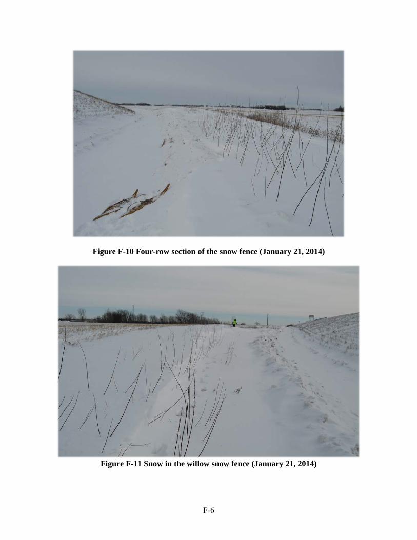
Figure F-10 Four-row section of the snow fence (January 21, 2014)

Figure F-11 Snow in the willow snow fence (January 21, 2014)

F-6

F-7

Figure F-12 Sprouting of the willows after spring coppice (May 22, 2014)

Figure F-13 Eric Ogdahl standing in a four-row section of the snow fence (August 8, 2014)

Figure F-14 Willow growth in Study 2 plots (Chapter 3) at the Southern Research and Outreach Center (August 9, 2014)

F-8

Figure F-15 Snow drifts in the snow fence (November 22, 2014)

Figure F-16 Snow drifts forming downwind of the snow fence (November 22, 2014)

F-9

Figure F-17 Snow drifts in the snow fence (January 15, 2015)

Figure F-18 Measuring snow drift depth downwind of snow fence (January 15, 2015)

F-10

Figure F-19 Close-up of graduated PVC tube for measuring drift depth (marked in centimeters) (January 15, 2015)

F-11

Figure F-20 The willow living snow fence (March 3, 2015)

Figure F-21 Snow fence willows in bloom (April 14, 2015)

F-12

Figure F-22 A moth visiting willow flowers (April 14, 2015)

Figure F-23 Two-row section of snow fence in bloom (April 14, 2015)

F-13

Figure F-24 Four-row section of snow fence in bloom (April 14, 2015)

Figure F-25 Four-row plot of willow variety ‘S365’ in the snow fence (May 20, 2015)

F-14

Figure F-26 Willow snow fence growth (orange post near center is approximately 5 feet tall) (September 3, 2015)

Figure F-27 Willow variety ‘Fish Creek’ in the snow fence next to corn (orange post is

about 5 feet tall) (September 3, 2015)

F-15

F-16

Figure F-28 Willow growth at Study 2 plots (Chapter 3) at the Southern Research and Outreach Center (September 3, 2015)

assessing the use of shrub-willows for living snow … for living snow fences in minnesota. ......

Documents