arrowtooth flounder by benjamin j. turnock, thomas k
TRANSCRIPT

ARROWTOOTH FLOUNDER
by Benjamin J. Turnock, Thomas K. Wilderbuer and Eric S. Brown
SUMMARY
Catch and fishery length data for 2001 were updated and 2002 catch and fishery length data were added to the model. An age-based model was used with the same configuration as the 2001 assessment, except an ascending logistic selectivity curve was used for the survey instead of a smooth selectivity function. The fishery selectivities were estimated using a smooth function as in past assessment models. Natural mortality for males was set higher than for females as in previous assessments, to obtain a sex ratio of about 70% female in the population. Length composition data were fit using a fixed length-age transition matrix estimated from survey length at age data. Survey biomass estimates from Halibut trawl surveys in the 1960’s, groundfish trawl surveys in the 1970’s and NMFS triennial trawl surveys from 1984 to 2001 were included in the model. The estimated biomass from the model increased from about 320,000 t in 1961 to a high of about 1,815,500 t in 2002. The 2003 ABC using F40% was 155,139 t. OFL using F35% was 181,394 t. The 2002 ABC using F40% was 146,264 t. Catch through 5 October 2002 was 19,009 t, similar to the 2001 catch of 19,964 t.

INTRODUCTION
Arrowtooth flounder (Atheresthes stomias) are currently the most abundant groundfish species in the Gulf of Alaska. Research has been conducted on their commercial utilization (Greene and Babbitt, 1990, Wasson et al., 1992, Porter et al., 1993, Reppond et al., 1993, Cullenberg 1995), however, arrowtooth flounder are currently of low value and most are discarded. In 1990, the North Pacific Fisheries Management Council separated arrowtooth flounder for management purposes from the flatfish assemblage, which at the time included all flatfish. Although arrowtooth flounder are presently of limited economic importance as a fisheries product, trophic studies (Yang 1993, Hollowed, et al. 1995, Hollowed et al. 2000) suggest they may be an important component in understanding the dynamics of the Gulf of Alaska benthic ecosystem. The majority of the prey by weight of arrowtooth larger than 40 cm was pollock, the remainder consisting of herring, capelin, euphausids, shrimp and cephalopods (Yang 1993). The percent of pollock in the diet of arrowtooth flounder increases for sizes greater than 40 cm. Arrowtooth flounder 15 cm to 30 cm consume mostly shrimp, capelin, euphausiids and herring, with small amounts of pollock and other miscellaneous fish. Groundfish predators include Pacific cod and Halibut. Arrowtooth flounder occur from central California to the Bering Sea, in waters from about 20m to 800m, although CPUE from survey data is highest in 100m to 300m. Information concerning stock structure is not currently available. Migration patterns are not well known for arrowtooth flounder, however, there is some indication that arrowtooth flounder move into deeper water as they grow, similar to other flatfish (Zimmerman and Goddard 1996).
CATCH HISTORY Prior to 1990, flatfish catch in the Gulf of Alaska was reported as an aggregate of all species. The bottom trawl fishery in the Gulf of Alaska primarily targets on rock, rex and Dover sole. The best estimate of annual arrowtooth catch since 1960 was calculated by multiplying the proportion of arrowtooth in observer sampled flatfish catches in recent years (nearly 50%) by the reported flatfish catch (1960-77 from Murai et al. 1981 and 1978-93 from Wilderbuer and Brown 1993) (Table 4.1). Catch through 5 October 2002 was 19,009 t, similar to the 2001 catch of 19,964 t, however, a decrease from the 2000 catch of 24,252 t. Total allowable catch for 2002 was 8,000 t for the Western GOA, 5,000 t for the Eastern GOA, and 25,000 t for the Central GOA. Table 4.2 documents annual research catches (1977 - 2001) from NMFS longline, trawl, and echo integration trawl surveys. Substantial amounts of flatfish are discarded overboard in the various trawl target fisheries. The following estimates of retained and discarded catch (t) since 1991, were calculated from discard rates observed from at-sea sampling and industry reported retained catch.

Year Discards Retained Percent retained1991 2,174 19,896 10%1992 498 22,629 2%1993 1,488 22,565 6%1994 458 22,011 2%1995 2,275 16,153 12%1996 5,438 17,093 24%1997 2,985 13,442 18%1998 2,057 10,943 15.80%1999 4,265 11,943 26.30%2000 9,938 13,044 43.20%2001 6619 13345 33.15%2002 10,032 10,381 49.15%
Under current fishing practices, arrowtooth flounder are mostly discarded when caught, although the percent retained has increased from below 10% in the early 1990’s to 49% in 2002.
ABUNDANCE AND EXPLOITATION TRENDS
The survey biomass estimates used in this assessment are from International Pacific Halibut Commission (IPHC) trawl surveys, NMFS groundfish surveys, and NMFS triennial surveys (Table 4.3). Biomass estimates from the surveys in the 1960’s and 1970’s were analyzed using the same strata and methods as the triennial survey (Brown 1986). The data from the 1961 and 1962 IPHC surveys were combined to provide total coverage of the GOA area. The NMFS surveys in 1973 to 1976 were also combined to provide total coverage of the survey area. However, sample sizes were lower in the 1970’s surveys (403 hauls, Table 4.3) than for other years, and some strata had less than 3 hauls. The IPHC and NMFS 1970’s surveys used a 400 mesh Eastern trawl, while the triennial surveys used a noreastern trawl. The trawl used in the early surveys had no bobbin or roller gear, which would cause the gear to be more in contact with the bottom than current trawl gear. Also the locations of trawl sites may have been restricted to smooth bottoms in the earlier surveys because the trawl could not be used on rough bottoms. Selectivity of the different surveys is assumed to be equal. There is limited size composition data for the 1970’s surveys but none for the 1960’s surveys. Catchability (Q) was assumed to be 1.0. NMFS has conducted studies to estimate the escapement under the triennial survey net, and will estimate herding into the net from future experiments. The percent of arrowtooth flounder caught that were in the path of the net varies by size from about 40% to 50% at 20-25 cm to about 95% at greater than 40cm(Peter Munro, pers. Comm.). This results in a Q that is close to 1.0. The herding component will result in a lower population biomass than survey biomass, however is unknown at this time. The 400 mesh eastern trawl used in the 1960’s and 1970’s surveys was estimated to be 1.61 times as efficient at catching arrowtooth flounder than the noreastern trawl used in the NMFS triennial surveys (Brown, in prep). The 1960’s and 1970’s survey abundance estimates have been lowered by dividing by 1.61. A cv of 0.2 for the efficiency estimate was assumed since a variance has not been estimated at this time. Survey abundance estimates were low in the 1960’s and 1970’s, increasing from about 146,000 t in 1975 to about 1,640,000 t in 1996, declining to 1,262,797 t in 1999, then increasing to about 1,622,000 t in 2001. The 2001 survey did not cover the eastern Gulf of Alaska. The average biomass estimated for the 1993 to 1999 surveys was used to

estimate the biomass in the eastern Gulf for 2001 (Table 4.4). The eastern gulf biomass has been between 14% and 22% of the total biomass for the 1993-1999 surveys.
ANALYTIC APPROACH
Model Structure
The model structure is developed following Fournier and Archibald’s (1982) methods, with many similarities to Methot (1990). We implemented the model using automatic differentiation software developed as a set of libraries under C++(ADModel Builder). ADModel Builder can estimate a large number of parameters in a non-linear model using automatic differentiation software extended from Greiwank and Corliss(1991) and developed into C++ class libraries. This software provides the derivative calculations needed for finding the objective function via a quasi-Newton function minimization routine(e.g., Press et al. 1992). The model implementation language (ADModel Builder) gives simple and rapid access to these routines and provides the ability to estimate the variance-covariance matrix for all parameters of interest. Details of the population dynamics and estimation equations, description of variables and likelihood equations are presented in Appendix A (Tables A.1, A.2 and A.3) . There were a total of 124 parameters estimated in the model (Table A.4). The 22 selectivity parameters estimated in the model were constrained so that the number of effectively free parameters would be less than the total of 124. There were 40 fishing mortality deviates in the model which were constrained to be small to fit the observed catch closely. The instantaneous natural mortality rate, catchability for the survey and the Von Bertalanffy growth parameters were fixed in the model (Table A.5).
Model assumptions
Weights used on the likelihood values were 1.0 for the survey length, survey age data and the survey biomass (simply implying that the variances and sample sizes specified for each data component were approximately correct). A weight of 0.25 was used for the fishery length data. The fishery length data is essentially from bycatch and in some years has low sample sizes. A lower weight on the fishery length data allows the model to fit the survey data components better. The estimated length at age relationship is used to convert population age compositions to estimated size compositions. The current model estimated size compositions using a fixed length-age transition matrix estimated from the 1984 through 1996 survey data combined. The distribution of lengths within ages was assumed to be normal with cv’s estimated from the length at age data of 0.06 for younger ages and 0.05 for older ages. Size bins were 2 cm starting at 24 cm, 3 cm bins from 40 cm to 69cm, one 5 cm bin from 70 cm to 74 cm, then a 75+cm bin. There were 13 age bins from 3 to 14 by 1 year interval, and ages over 15 accumulated in the last bin, 15+. Recruitment in the last three years (2000,2001,2002) of the model were constrained to be close to the mean recruitment over the 20 year period from 1981 to 1999, due to the lack of data to estimate recruitments for those years.
Data Sources The model simulates the dynamics of the population and compares the expected values of the population characteristics to those observed from surveys and fishery sampling programs.

The following data sources were used in the model: Data component YearsFishery catch 1960-2002IPHC trawl survey biomass and S.E. 1961-1962NMFS exploratory research trawl survey biomass and S.E.
1973-1976
NMFS triennial trawl survey biomass and S.E. 1984,1987,1990,1993,1996,1999,2001 Fishery size compositions 1977-1981,1984-1993,1995-2002NMFS survey size compositions 1975,1999,2001
NMFS triennial trawl survey age composition data
1984,1987,1990,1993,1996
Sample sizes for the fishery length data were adequate for the 1970’s and 1980’s. However, sample sizes in recent years have decreased. No length samples were collected in 1994. Otoliths from the 1984, 1987, 1990, 1993 and 1996 triennial trawl surveys were aged in 1998 and 1999 allowing the use of age compositions in the model (Table 4.5). Size composition data for the surveys are shown in Table 4.6.
Natural mortality, Age of recruitment, and Maximum Age The estimation of natural mortality rates for Gulf of Alaska arrowtooth flounder were analyzed using the methods of Alverson and Carney (1975), Pauly (1980), and Hoenig (1983) in the 1988 assessment (Wilderbuer and Brown 1989). The maximum age of female arrowtooth flounder otoliths collected was 23 years. Using Hoenig’s empirical regression method (Hoenig 1983) M would be estimated at 0.18. There are fewer males than females in the 15+ age group, with the maximum age for males varying between 14 and 20 years from different survey years. Natural Mortality with a maximum age of 14 years and 20 years was estimated at 0.30 and 0.21 respectively using Hoenig’s method. Natural mortality was fixed at 0.2 for females. A higher natural mortality for males was used to fit the age and size composition data, which are about 70% female. A value of M=0.35 for males was chosen so that the survey selectivities for males and females both reached a maximum selectivity close to 1.0. A likelihood profile on male natural mortality resulted in a mean and mode of 0.354 with 95% confidence intervals of 0.32 to 0.38 (Figure 4.14). Model runs examining the effect of different natural mortality values for male arrowtooth flounder can be found in the Appendix of the 2000 SAFE. The prevalence of females in the survey and fishery data could be the result of lower availability for males or higher natural mortality. If lower availability is assumed, then the 3+ biomass and ABC will be higher, even though the F40% and female spawning biomass will remain unchanged. However, the data point towards a higher natural mortality rather than lower availability for males, although lower availability cannot be ruled out without further research. The age composition of males shows fewer males relative to females as fish increase in age, which would be the case for higher M for males. However, if males became unavailable to the gear at a fairly constant rate as they aged, the same effect would result. The survey and fishery data in both the Bering sea and GOA have about 70% female in the catches, which also points towards a higher M for males. Most of the abundance of arrowtooth flounder from survey data occurs at depths less than 300 meters. The fraction female is fairly constant at about 65% to 74% for depths up to 500 meters (Figure 4.15). In the deepest areas, covered in the 1999 and 1987 surveys, the fraction female was variable, being about 0.5 in 1987 and 0.83 in 1999.

The data by depth do not indicate that males in any depth strata are less available than in other depth strata. Age at recruitment was set at three in the model due to the small number of fish caught at younger ages.
Weight at Age The weight-length relationship for arrowtooth flounder is, W = .003915 L 3.2232 , for both sexes combined where weight is in grams and length in centimeters.
Selectivity
The shape of the selectivity curve for the fishery was constrained to be monotonically increasing with age using a smooth function (Figure 4.1). Survey selectivities were modeled using a two parameter ascending logistic function. The selectivities by age were estimated separately for females and males. The differential natural mortality and selectivities by sex resulted in a predicted fraction female of about 0.70, which is close to the fraction female in the fishery and survey length and age data.
Growth
In the growth equation shown below, Linf was estimated as 101.5 cm for females and 54 cm for males(Figure 4.2). The length at age 2 (L1) for both sexes was estimated at 20 cm and k was 0.077 for females and 0.22 for males from the survey age and length data in 1984 through 1996.
))1(exp(*)( max1max −−−+= tkLLLLt .
The mean length at age data from the surveys show no trends over time for females (Table 4.8 and Figure 4.3). Males were smaller in 1984, however other years are similar (Table 4.7 and Figure 4.4).
Maturity
Length at 50% mature was estimated at 47 cm with a logistic slope of -0.3429 from arrowtooth sampled in hauls that occurred in September from the 1993 bottom trawl survey (Zimmerman in review). Arrowtooth flounder are batch spawners, spawning from fall to winter off Washington State at depths greater than 366 m (Rickey 1995). There was some indication of migration of larger fish to deeper water in winter and shallower water in summer from examination of fisheries data off Washington, however, discarding of fish may confound observations (Rickey 1995). Length at 50% mature from survey data in 1992 off Washington was 36.8 cm for females and 28.0 cm for males, with logistic slopes of -0.54 and -0.893 respectively (Rickey 1995). Oregon arrowtooth flounder had length at 50% mature of 44 cm for females and 29 cm for males (Rickey 1995). Spawning fish were found in depths from 108m to 360m in March to August in the Gulf of Alaska (Hirshberger and Smith 1983) from analysis of trawl surveys from 1975 to 1981. Most observations of spawning fish were found in the northeastern Gulf, off Prince William Sound, off Cape St. Elias, and Icy Bay.

RESULTS
Fits to the size composition data from the fishery are shown in Figures 4.5 for females and Figure 4.6 for males. The survey length data in 1975 were fit well by the model, however, the length data from the 1999 and 2001 surveys lacked larger female fish that are estimated by the model (Figures 4.7 and 4.8). The high recruitments in the 1980’s and early 1990’s and the low fishing mortalities resulted in more large older female fish in the estimated population than were found in the 1999 and 2001 surveys. The survey length data for males is fit well (Figure 4.8). The survey age data in 1993 and 1996 indicate some accumulation of older female fish in the 15+ age bin, which is slightly overestimated by the model (Figure 4.9).
Model estimates of biomass
The model estimates of age 3+ biomass increased from a low of about 320,000 t in 1961 to a high of about 1,815,500 t in 2002 (Table 4.9 and Figure 4.11). The 2001 survey biomass estimate was 1,621,890 t, an increase from the 1999 survey biomass estimate of 1,262,797 t.
Model estimates of recruitment
The model estimates of age 3 recruits increase in the 1970’s and 1980’s then decrease in the 1990’s (Table 4.9 and Figure 4.12). Recruitment in 2000 to 2002 was constrained to be close to the historical harmonic mean recruitment for 1981 to 1999. This was done as a precautionary approach since the harmonic mean recruitment is less than the arithmetic mean recruitment.
Spawner-Recruit Relationship No spawner-recruit curve was used in the Model. Recruitments were estimated as deviations from a mean value on a log scale.
REFERENCE FISHING MORTALITY RATES AND YIELDS Reliable estimates of biomass, B35%, F35% and F40%, are available, and current biomass is greater than B40%. Therefore, arrowtooth flounder is in tier 3a of the ABC and overfishing definitions. Under this definition, Fofl= F35%, and FABC is less than or equal to F40%.
Yield for 2003 using F40% = 0.14 was estimated at 155,139 t. Yield at F35% = 0.165 was
estimated at 181,394 t. The fishing mortality rates for 2003 are slightly higher than in the 2002 assessment (F40%
= 0.134, F35% = 0.159) due to changes in fishery selectivities. Survey selectivities were estimated using a two parameter logistic function rather than a smooth function in the 2002 assessment, which resulted in a small change in the fishery selectivities.
MAXIMUM SUSTAINABLE YIELD
Since there is no estimate of the spawner-recruit relationship for arrowtooth flounder, no attempt has been made to estimate MSY. However, using the projection model described in the next section, spawning biomass with F=0 was estimated at 1,236,240 t. B35% (equilibrium spawning biomass with fishing at F35%) is estimated at 432,683 t.

PROJECTED CATCH AND ABUNDANCE
A standard set of projections is required for each stock managed under Tiers 1, 2, or 3 of Amendment 56. This set of projections encompasses seven harvest scenarios designed to satisfy the requirements of Amendment 56, the National Environmental Protection Act, and the Magnuson-Stevens Fishery Conservation and Management Act (MSFCMA). For each scenario, the projections begin with the vector of 2002 numbers at age estimated in the assessment. This vector is then projected forward to the beginning of 2003 using the schedules of natural mortality and selectivity described in the assessment and the best available estimate of total (year-end) catch for 2002. In each subsequent year, the fishing mortality rate is prescribed on the basis of the spawning biomass in that year and the respective harvest scenario. In each year, recruitment is drawn from an inverse Gaussian distribution whose parameters consist of maximum likelihood estimates determined from recruitments estimated in the assessment. Spawning biomass is computed in each year based on the time of peak spawning and the maturity and weight schedules described in the assessment. Total catch is assumed to equal the catch associated with the respective harvest scenario in all years. This projection scheme is run 1000 times to obtain distributions of possible future stock sizes, fishing mortality rates, and catches. Five of the seven standard scenarios will be used in an Environmental Assessment prepared in conjunction with the final SAFE. These five scenarios, which are designed to provide a range of harvest alternatives that are likely to bracket the final TAC for 2003, are as follow (“max FABC” refers to the maximum permissible value of FABC under Amendment 56):
Scenario 1: In all future years, F is set equal to max FABC. (Rationale: Historically, TAC has been constrained by ABC, so this scenario provides a likely upper limit on future TACs.)
Scenario 2: In all future years, F is set equal to a constant fraction of max FABC, where this fraction is equal to the ratio of the FABC value for 2003 recommended in the assessment to the max FABC for 2003. (Rationale: When FABC is set at a value below max FABC, it is often set at the value recommended in the stock assessment.)
Scenario 3: In all future years, F is set equal to 50% of max FABC. (Rationale: This scenario provides a likely lower bound on FABC that still allows future harvest rates to be adjusted downward when stocks fall below reference levels.)
Scenario 4: In all future years, F is set equal to the 1995-1999 average F. (Rationale: For some stocks, TAC can be well below ABC, and recent average F may provide a better indicator of FTAC than FABC.)
Scenario 5: In all future years, F is set equal to zero. (Rationale: In extreme cases, TAC may be set at a level close to zero.)
Two other scenarios are needed to satisfy the MSFCMA’s requirement to determine whether a stock is currently in an overfished condition or is approaching an overfished condition. These two scenarios are as follow (for Tier 3 stocks, the MSY level is defined as B35%):
Scenario 6: In all future years, F is set equal to FOFL. (Rationale: This scenario determines whether a stock is overfished. If the stock is expected to be above ½ of its MSY level in 2003 and above its MSY level in 2013 under this scenario, then the stock is not overfished.)
Scenario 7: In 2003 and 2004, F is set equal to max FABC, and in all subsequent years, F is set equal to FOFL. (Rationale: This scenario determines whether a stock is approaching an overfished condition. If the stock is expected to be above its MSY level in 2015 under this scenario, then the stock is not approaching an overfished condition.)
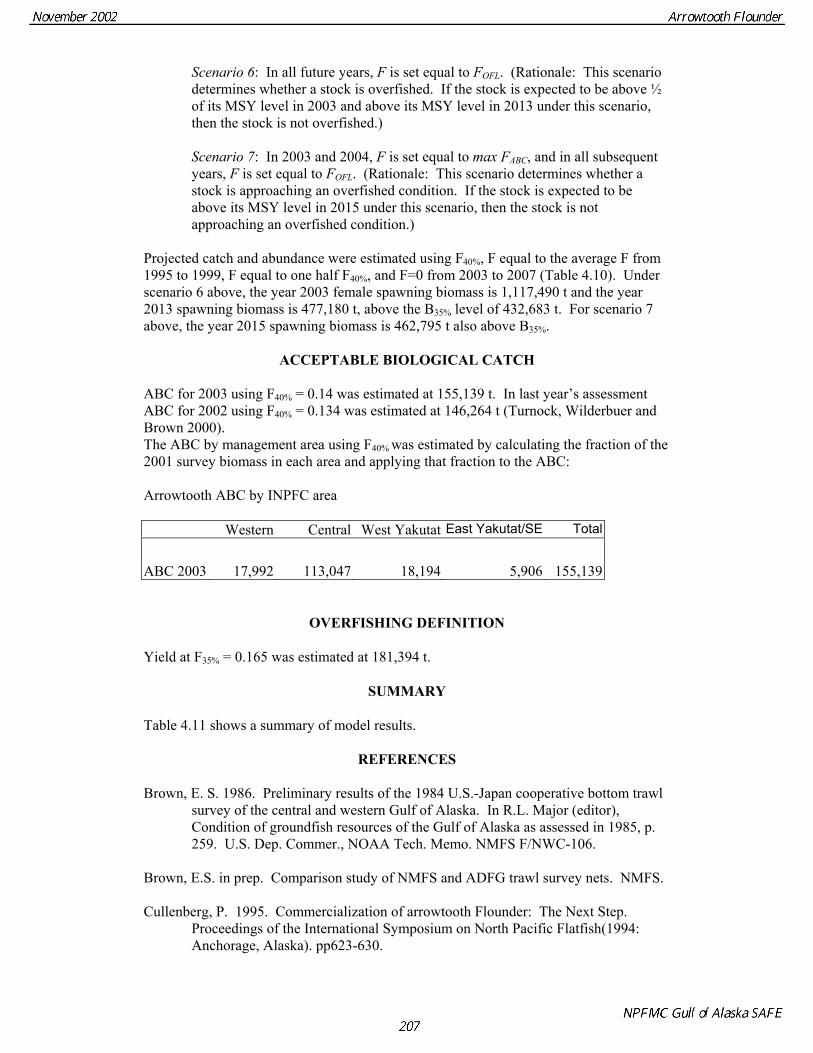
Projected catch and abundance were estimated using F40%, F equal to the average F from 1995 to 1999, F equal to one half F40%, and F=0 from 2003 to 2007 (Table 4.10). Under scenario 6 above, the year 2003 female spawning biomass is 1,117,490 t and the year 2013 spawning biomass is 477,180 t, above the B35% level of 432,683 t. For scenario 7 above, the year 2015 spawning biomass is 462,795 t also above B35%.
ACCEPTABLE BIOLOGICAL CATCH ABC for 2003 using F40% = 0.14 was estimated at 155,139 t. In last year’s assessment ABC for 2002 using F40% = 0.134 was estimated at 146,264 t (Turnock, Wilderbuer and Brown 2000). The ABC by management area using F40% was estimated by calculating the fraction of the 2001 survey biomass in each area and applying that fraction to the ABC: Arrowtooth ABC by INPFC area
Western Central West Yakutat East Yakutat/SE Total
ABC 2003 17,992 113,047 18,194 5,906 155,139
OVERFISHING DEFINITION
Yield at F35% = 0.165 was estimated at 181,394 t.
SUMMARY
Table 4.11 shows a summary of model results.
REFERENCES Brown, E. S. 1986. Preliminary results of the 1984 U.S.-Japan cooperative bottom trawl
survey of the central and western Gulf of Alaska. In R.L. Major (editor), Condition of groundfish resources of the Gulf of Alaska as assessed in 1985, p. 259. U.S. Dep. Commer., NOAA Tech. Memo. NMFS F/NWC-106.
Brown, E.S. in prep. Comparison study of NMFS and ADFG trawl survey nets. NMFS. Cullenberg, P. 1995. Commercialization of arrowtooth Flounder: The Next Step.
Proceedings of the International Symposium on North Pacific Flatfish(1994: Anchorage, Alaska). pp623-630.

Clark, W. G. 1992. Alternative target levels of spawning biomass per recruit. Unpubl. manuscr., 5 p. Int. Pac. Hal. Comm., P.O. Box 95009, Seattle, WA 98145.
Fournier, D.A. and C.P. Archibald. 1982. A general theory for analyzing catch-at-age
data. Can. J.Fish.Aquat.Sci. 39:1195-1207. Greene, D.H., and J.K. Babbitt. 1990. Control of muscle softening and protease-parasite
interactions in arrowtooth flounder, Atheresthes stomias. J. Food Sci. 55(2): 579-580.
Greiwank, A. and G.F. Corliss(eds). 1991. Automatic differentiation of algorithms: theory, implementation and application. Proceedings of the SIAM Workshop on the Automatic Differentiation of Algorithms, held Jan. 6-8, Breckenridge, CO. Soc. Indust. And Applied Mathematics, Philadelphia.
Hirshberger, W.A., and G.B. Smith. 1983. Spawning of twelve groundfish species in the
Alaska and Pacific coast regions, 1975-81. U.S. Dep. Commer., NOAA Tech. Memo. NMFS F/NWC:44, 50p.
Hoenig, J. 1983. Empirical use of longevity data to estimate mortality rates. Fish. Bull.
82: 898-903. Hollowed, A.B., E. Brown, P. Livingston, B. Megrey, I. Spies and C. Wilson. 1995.
Walleye Pollock. In: Stock Assessment and Fishery Evaluation Report for the 1996 Gulf of Alaska Groundfish Fishery. 79 p. Gulf of Alaska Groundfish Plan Team, North Pacific Fishery Management Council, P. O. Box 103136, Anchorage, Ak 99510.
Hollowed, A. B., J. N. Ianelli, and P. A. Livingston. 2000. Including predation mortality
in stock assessments: A case study involving Gulf of Alaska walleye pollock. ICES Journal of Marine Science, 57, pp. 279-293.
Methot, R. D. 1990. Synthesis model: An adaptable framework for analysis of diverse
stock assessment data. Int. N. Pac. Fish. Comm. Bull. 50:259-277. Murai, S., H. A. Gangmark, and R. R. French. 1981. All-nation removals of groundfish,
Herring, and shrimp from the eastern Bering Sea and northeast Pacific Ocean, 1964-80. NWAFC report. 40 p.
Pauly, D. 1980. On the interrelationships between natural mortality, growth parameters,
and mean environmental temperature in 175 fish stocks. J. Cons. Int. Explor. Mer, 39:175-192.
Porter, R.W., B.J. Kouri, and G. Kudo. 1993. Inhibition of protease activity in muscle
extracts and surimi from Pacific Whiting, Merluccius productus, and arrowtooth flounder, Atheresthes stomias. Mar. Fish. Rev. 55(3):10-15.
Press, W.H., S.A. Teukolsky, W.T.Vetterling, B.P. Flannery. 1992. Numerical Recipes
in C. Second Ed. Cambridge Univ. Press. 994 p. Reppond, K.D., D.H. Wasson, and J.K. Babbitt. 1993. Properties of gels produced from
blends of arrowtooth flounder and Alaska pollock surimi. J. Aquat. Food Prod. Technol., vol. 2(1):83-98.

Rickey, M.H. 1995. Maturity, spawning, and seasonal movement of arrowtooth flounder, Atheresthes stomias, off Washington. Fish. Bull., U.S. 93(1):127-138.
Turnock, B.J., T.K. Wilderbuer and E.S. Brown. 1996. Arrowtooth Flounder. In Stock
Assessment and Fishery Evaluation Report for the 1997 Gulf of Alaska Groundfish Fishery. 30 p. Gulf of Alaska Groundfish Plan Team, North Pacific Fishery Management Council, P. O. Box 103136, Anchorage, Ak 99510.
Turnock, B.J., T.K. Wilderbuer and E.S. Brown. 1999. Arrowtooth Flounder. In Stock
Assessment and Fishery Evaluation Report for the 2000 Gulf of Alaska Groundfish Fishery. 30 p. Gulf of Alaska Groundfish Plan Team, North Pacific Fishery Management Council, P. O. Box 103136, Anchorage, Ak 99510.
Turnock, B.J., T.K. Wilderbuer and E.S. Brown. 2000. Arrowtooth Flounder. In Stock
Assessment and Fishery Evaluation Report for the 2001 Gulf of Alaska Groundfish Fishery. 30 p. Gulf of Alaska Groundfish Plan Team, North Pacific Fishery Management Council, P. O. Box 103136, Anchorage, Ak 99510.
Wasson, D.H., K.D. Reppond, J.K. Babbitt, and J.S. French. 1992. Effects of additives
on proteolytic and functional properties of arrowtooth flounder surimi. J. Aquat. Food Prod. Technol., vol. 1(3/4):147-165.
Wilderbuer, T. K., and E. S. Brown. 1989. Flatfish. In T. K. Wilderbuer (editor),
Condition of groundfish resources of the Gulf of Alaska as assessed in 1988. p. 199-218. U.S. Dep. Commer., NOAA Tech. Memo, NMFS F/NWC-165.
Wilderbuer, T. K., and E. S. Brown. 1995. Flatfish. In Stock Assessment and Fishery
Evaluation Report for the 1996 Gulf of Alaska Groundfish Fishery. 21 p. Gulf of Alaska Groundfish Plan Team, North Pacific Fishery Management Council, P. O. Box 103136, Anchorage, Ak 99510.
Yang, M. S. 1993. Food Habits of the Commercially Important Groundfishes in the Gulf
of Alaska in 1990. U.S. Dept. Commer., NOAA Tech. Memo. NMFS-AFSC-22, 150p.
Zimmerman, M. in review. Maturity and fecundity of arrowtooth flounder, Atheresthes
stomias, from the Gulf of Alaska. Zimmerman, M., and P. Goddard. 1996. Biology and distribution of arrowtooth flounder,
Atheresthes stomias, and Kamchatka flounders (A. evermanni) in Alaskan waters. Fish. Bull., U.S.

Table 4.1. Catch of arrowtooth flounder in the Gulf of Alaska from 1964 to 5 October, 2002. Year Catch(mt) 1964 514 1965 514 1966 2,469 1967 2,276 1968 1,697 1969 1,315 1970 1,886 1971 1,185 1972 4,477 1973 10,007 1974 4,883 1975 2,776 1976 3,045 1977 9,449 1978 8,409 1979 7,579 1980 7,848 1981 7,433 1982 4,639 1983 6,331 1984 3,457 1985 1,539 1986 1,221 1987 4,963 1988 5,138 1989 2,584 1990 7,706 1991 10,034 1992 15,970 1993 15,559 1994 23,560 1995 18,428 1996 22,583 1997 16,319 1998 12,975 1999 16,207 2000 24,252 2001 19,964 2002 19,009

Table 4.2. Catches from NMFS research cruises from 1977 to 2002.
Year Catch (mt) 1977 29.3 1978 30.6 1979 38.9 1980 36.7 1981 151.5 1982 90.2 1983 61.4 1984 223.9 1985 149.4 1986 179.0 1987 297.4 1988 22.0 1989 64.1 1990 228.1 1991 27.7 1992 32.1 1993 255.4 1994 36.7 1995 173.5 1996 154.6 1997 40.6 1998 115.6 1999 101.5 2000 24.0 2001 83.9 2002 11.0
Table 4.3. Biomass estimates and standard errors from bottom trawl surveys. Survey Biomass(mt) s.e. Hauls IPHC 1961-1962 283,799 61,515 1,172 NMFS groundfish 1973-1976 145,744 33,531 403 NMFS triennial 1984 979,335 71,209 930 NMFS triennial 1987 979,957 74,673 783 NMFS triennial 1990 1,922,107 239,150 708 NMFS triennial 1993 1,585,040 101,160 776 NMFS triennial 1996 1,639,671 114,792 804 NMFS triennial 1999 1,262,797 99,329 764 NMFS triennial 2001 1,621,892 178,408 489 _ Table 4.4. Survey biomass estimates (mt) for 1993 to 2001 by area. The 2001 survey biomass for the eastern gulf was estimated by using the average of the 1993 to 1999 biomass estimates in the eastern gulf.
Area 1993 1996 1999 2001Western 212,332 202,594 143,374 188,100 Central 1,117,361 1,176,714 845,176 1,181,848 Eastern 222,015 260,324 273,490 251,943*

Tabl
e 4.
5. A
ge d
ata
from
trie
nnia
l sur
veys
in 1
984
thro
ugh
1996
. Th
e nu
mbe
rs a
re p
erce
ntag
es, w
here
the
fem
ale
plus
the
mal
e nu
mbe
rs a
dd to
100
with
in a
ye
ar.
fem
ales
1
2 3
4 5
67
89
1011
1213
14
1516
1718
1920
2122
23
1984
0.
01
0.00
3.
61
5.87
10.
37 1
5.82
8.55
5.41
2.30
1.65
1.17
1.25
0.70
0.83
2.
910.
000.
000.
000.
000.
000.
000.
000.
00
1987
0.
00
1.93
7.
86
9.18
7.
05
8.00
5.23
11.8
16.
983.
370.
910.
981.
690.
27
0.30
0.00
0.00
0.00
0.00
0.00
0.00
0.00
0.00
19
90
0.00
2.
81
5.48
6.
50 1
1.40
11.
076.
527.
344.
382.
413.
772.
291.
280.
74
0.84
0.64
0.96
0.61
0.21
0.00
0.16
0.00
0.00
19
93
0.13
4.
40
6.54
6.
03
6.44
7.
658.
127.
889.
604.
602.
542.
771.
631.
05
0.46
0.23
0.33
0.13
0.02
0.02
0.02
0.00
0.01
19
96
0.03
3.
93
5.71
6.
76
6.83
8.
748.
797.
177.
848.
352.
271.
280.
890.
55
0.14
0.14
0.00
0.01
0.00
0.01
0.00
0.00
0.00
m
ales
1984
0.
00
0.00
0.
56
4.42
5.
31
4.05
5.10
5.44
3.76
2.72
2.46
1.66
1.05
0.88
2.
150.
000.
000.
000.
000.
000.
000.
000.
00
1987
0.
00
0.00
8.
10
6.95
8.
08
3.62
2.40
2.44
0.45
0.00
0.69
1.03
0.35
0.35
0.
000.
000.
000.
000.
000.
000.
000.
000.
00
1990
0.
00
2.51
3.
53
4.90
5.
10
4.42
4.54
0.67
2.33
1.27
1.24
0.00
0.00
0.08
0.
000.
000.
000.
000.
000.
000.
000.
000.
00
1993
0.
08
2.90
3.
75
2.53
2.
70
6.70
3.20
2.63
1.93
1.08
0.77
0.45
0.24
0.12
0.
090.
110.
000.
040.
000.
090.
000.
000.
00
1996
0.
07
2.64
3.
47
3.54
3.
70
5.82
2.88
4.04
1.48
1.09
1.06
0.50
0.12
0.05
0.
050.
000.
050.
000.
000.
000.
000.
000.
00
6 Tabl
e 4.
6. L
engt
h da
ta fr
om tr
ienn
ial s
urve
ys in
198
4 th
roug
h 20
01.
The
num
bers
are
per
cent
ages
, whe
re th
e fe
mal
e pl
us th
e m
ale
num
bers
add
to 1
00 w
ithin
a
year
.
Len
gth(
cm)
22
24
26
28
30
32
34
3638
4043
4649
52
55
5861
6467
7075
+Fe
mal
e
19
75 4
.99
4.38
4.7
7 5.
07
4.59
4.
58
4.83
4.89
4.05
4.02
3.21
2.79
2.37
1.49
1.
04
0.67
0.38
0.34
0.21
0.14
0.01
1999
1.9
0 1.
78 2
.89
3.34
3.
18
3.35
3.
683.
563.
254.
303.
984.
815.
927.
46
7.26
4.
111.
841.
060.
690.
530.
3320
01 4
.10
2.51
2.0
0 2.
66
3.21
2.
89
3.04
3.47
3.29
5.06
5.53
5.99
6.14
5.63
5.
76
4.18
2.32
1.39
1.00
1.29
0.36
Mal
e
19
75 3
.63
3.19
3.9
1 4.
72
4.69
4.
64
4.68
3.96
2.88
2.35
0.91
0.16
0.04
0.03
0.
02
0.01
0.01
0.00
0.00
0.00
0.00
1999
1.2
2 1.
14 1
.83
1.98
1.
93
1.91
2.
001.
952.
043.
314.
343.
761.
760.
24
0.05
0.
030.
000.
000.
000.
000.
0020
01 2
.46
1.36
1.5
5 2.
00
1.87
1.
82
1.87
1.88
1.84
3.31
3.27
3.02
1.62
0.28
0.
01
0.00
0.00
0.00
0.00
0.00
0.00

Table 4.7. Mean length (cm) at age for male arrowtooth flounder from triennial surveys 1984 through 1996.
1984 1987 1990 1993 19961 0.0 0.0 0.0 15.8 14.52 0.0 23.8 0.0 21.4 20.73 22.3 28.4 28.6 27.6 26.34 26.0 33.1 33.6 31.9 34.05 29.9 36.9 37.2 36.9 35.36 33.6 41.1 39.4 40.9 41.17 36.1 41.2 41.8 42.2 43.68 37.8 42.5 43.7 44.3 44.79 39.3 42.8 44.5 45.7 46.9
10 40.1 0.0 45.3 45.5 46.911 41.7 42.5 46.2 46.2 48.112 42.6 42.9 0.0 48.8 49.113 42.9 45.0 0.0 47.1 49.314 44.3 45.0 51.0 40.0 51.015 47.5 0.0 0.0 48.0 52.016 0.0 0.0 0.0 47.0 0.017 0.0 0.0 0.0 0.0 51.018 0.0 0.0 0.0 52.0 0.019 0.0 0.0 0.0 0.0 0.020 0.0 0.0 0.0 48.0 0.0
Table 4.8. Mean length (cm) at age for female arrowtooth flounder from triennial surveys 1984 through 1996.
1984 1987 1990 1993 19961 0.0 0.0 0.0 15.4 13.32 0.0 23.0 22.6 21.5 21.53 25.2 30.1 27.9 27.6 26.34 31.5 35.3 33.2 32.5 32.95 38.0 38.6 38.1 39.4 37.46 42.3 44.9 43.5 41.7 42.17 46.6 47.2 45.4 46.5 46.68 50.8 50.1 49.1 48.5 49.79 54.0 51.7 51.7 52.5 53.6
10 56.7 50.4 55.8 55.6 54.811 58.9 50.2 58.3 55.8 59.212 60.8 51.5 58.3 55.9 63.813 62.8 55.2 58.5 61.5 64.714 63.9 51.0 63.8 59.7 68.215 66.8 57.0 56.2 60.5 73.716 0.0 0.0 60.8 67.2 68.317 0.0 0.0 74.7 64.4 0.018 0.0 0.0 73.4 69.1 81.019 0.0 0.0 63.0 76.7 0.020 0.0 0.0 0.0 70.6 82.021 0.0 0.0 70.0 81.2 0.022 0.0 0.0 0.0 0.0 0.023 0.0 0.0 0.0 79.0 0.0

Table 4.9. Estimated age 3+ population biomass(mt), female spawning biomass(mt) and age 3 recruits(1,000’s).
Year age 3+ biomass Female spawning biomass Age 3 recruits (1,000's)1961 320,430 192,084 84,9291962 329,685 201,629 80,2251963 334,933 208,437 74,0801964 338,075 213,321 76,8201965 339,021 216,757 73,5841966 339,190 218,895 77,1251967 336,665 217,942 78,5271968 334,820 216,079 83,3911969 335,126 214,187 91,9241970 338,681 212,540 105,8731971 344,217 210,696 114,8311972 360,139 210,139 169,0841973 387,843 207,871 247,5361974 432,923 202,924 359,8091975 506,036 205,019 447,1821976 565,363 214,667 272,2451977 633,702 233,659 344,1481978 688,553 262,433 293,3001979 736,014 305,853 255,8561980 783,348 356,831 281,1531981 845,490 405,754 401,1051982 912,398 450,883 413,6671983 961,337 492,687 270,4041984 1,008,970 531,617 301,4591985 1,075,980 576,593 420,7071986 1,157,650 630,560 473,9291987 1,252,230 683,750 545,0521988 1,314,410 710,355 461,1801989 1,376,160 740,780 440,1261990 1,438,820 774,727 491,4991991 1,481,630 810,679 426,1731992 1,526,870 851,778 472,7131993 1,600,280 893,845 659,5401994 1,655,710 929,400 519,3691995 1,678,000 943,691 459,0451996 1,703,760 965,572 452,2481997 1,725,450 996,554 431,8201998 1,760,080 1,037,870 505,4071999 1,794,340 1,079,200 482,7602000 1,808,480 1,099,790 456,0822001 1,810,040 1,104,870 463,1812002 1,815,540 1,113,830 449,072
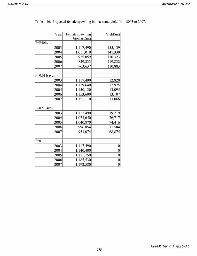
Table 4.10. Projected female spawning biomass and yield from 2003 to 2007.
Year Female spawning
biomass(mt)Yield(mt)
F=F40% 2003 1,117,490 155,1392004 1,011,010 141,3302005 925,059 130,3232006 839,233 119,8322007 763,637 110,883
F=0.011(avg F)
2003 1,117,490 12,8202004 1,129,640 12,9252005 1,150,120 13,0952006 1,153,600 13,1072007 1,151,110 13,066
F=0.5 F40%
2003 1,117,490 79,7192004 1,073,650 76,7172005 1,040,870 74,4162006 996,854 71,5842007 953,074 68,875
F=0
2003 1,117,490 02004 1,140,400 02005 1,171,750 02006 1,185,530 02007 1,192,580 0

Table 4.11. Summary of results of arrowtooth flounder assessment in the Gulf of Alaska. Natural Mortality 0.2 females 0.35 males Age of full(95%) selection 9 females, 12 males Reference fishing mortalities F40% 0.140 F35% 0.165 Biomass at MSY N/A Equilibrium unfished Spawning biomass 1,236,240 t B35% Spawning biomass fishing at F35% 432,683 t B40% Spawning biomass fishing at F40% 494,495 t Projected 2003 biomass Total(age 3+) 1,813,980 t Spawning 1,117,490 t Exploitable 1,302,000 t Overfishing level for 2003 181,394 t
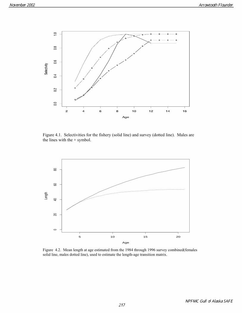
Figure 4.1. Selectivities for the fishery (solid line) and survey (dotted line). Males are the lines with the + symbol.
Age
Leng
th
5 10 15 20
020
4060
80
Figure 4.2. Mean length at age estimated from the 1984 through 1996 survey combined(females solid line, males dotted line), used to estimate the length-age transition matrix.
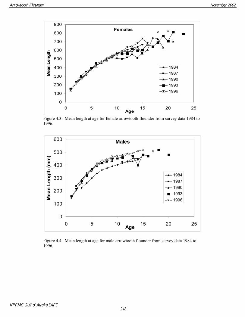
Figure 4.3. Mean length at age for female arrowtooth flounder from survey data 1984 to 1996. Figure 4.4. Mean length at age for male arrowtooth flounder from survey data 1984 to 1996.
Females
0
100
200
300
400
500
600
700
800
900
0 5 10 15 20 25Age
Mea
n Le
ngth
19841987199019931996
Males
0
100
200
300
400
500
600
0 5 10 15 20 25Age
Mea
n Le
ngth
(mm
)
19841987199019931996

Figure 4.5. Fit to the female fishery length composition data. Dotted line is predicted. 100-102 are years 2000-2002.

Figure 4.6. Fit to the male fishery length composition data. Dotted line is predicted. 100-102 are years 2000-2002.

Figure 4.7. Fit to the female survey length data. Dotted line is predicted. 101 is year 2001.
Figure 4.8. Fit to the male survey length data. Dotted line is predicted. 101 is year 2001.

Figure 4.9. Fit to the female survey age data. The last age group is 15+. Dotted line is predicted.
Figure 4.10. Fit to the male survey age data. The last age group is 15+. Dotted line is predicted.

Figure 4.11. Age 3+ biomass (solid line) and female spawning biomass (line with +) from 1984 to 2001. The approximate lognormal 95% confidence intervals shown underestimate the uncertainty because variance in natural mortality and survey Q as well as other fixed parameters are not accounted for.
Figure 4.12. Age 3 estimated recruitments (male plus female) in numbers from 1961 to 2002, with approximate 95% confidence intervals. Horizontal line is average recruitment.

Figure 4.13. Fit to survey biomass estimates with approximate 95% log-normal confidence intervals for the observed survey biomass estimates 1961 to 2001. Figure 4.14. Likelihood profile for estimating male natural mortality in the model. 95% confidence interval is 0.322 to 0.384. The mean and mode both equal 0.354.
Likelihood Profile
0
5
10
15
20
25
30
0.3 0.32 0.34 0.36 0.38 0.4
Male natural mortality
Prob
abili
ty D
ensi
ty
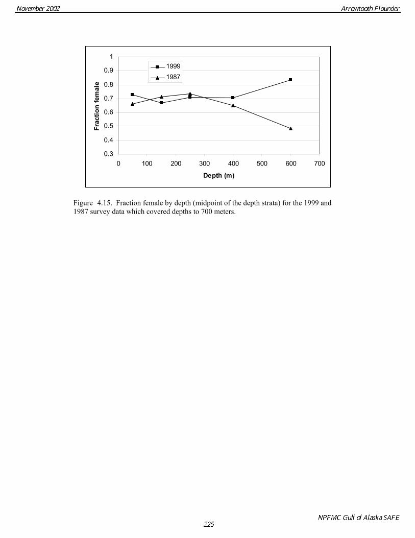
Figure 4.15. Fraction female by depth (midpoint of the depth strata) for the 1999 and 1987 survey data which covered depths to 700 meters.
0.3
0.4
0.5
0.6
0.7
0.8
0.9
1
0 100 200 300 400 500 600 700
Depth (m)
Frac
tion
fem
ale
19991987

Appendix A.
Table A.1. Model equations describing the populations dynamics.
teRRN ttτ
01, == ),0(~ 2Rt N στ Recruitment
atZ
at
atat Ne
ZF
C at,
,
,, )1( ,−−=
AaTt≤≤≤≤
11 Catch
atZatat eNN ,
,1,1−
++ =
AaTt<≤≤<
11
Numbers at age
ata
A
aat NwFSB ,
1φ∑
=
= Female spawning
biomass
AtAt ZAt
ZAtAt eNeNN ,1,
,1,,1−−
−+ += −
Tt ≤<1 Numbers in “plus” group
MFZ atat += ,, Total Mortality
∑=
=A
aatt CC
1,
Total Catch in numbers
CCp atat /,, = proportion at age in the catch
at
A
aatt CwY ,
1,∑
=
= Yield
teEsF tatatε
,, = ),0(~ 2Rt N σε
Fishing mortality
Sa for a = 3 to 13 selectivity – smooth monotonically increasing function for fishery
Sa for a = 3 to 13 selectivity –ascending logistic for survey
ats
A
aat NswQSB
at ,1
,∑=
= survey biomass, Q = 1.

Table A.2. Likelihood components.
[ ]2
1,, )log()log(∑
=
−T
tpredtobst CC
Catch using a lognormal distribution.
)log(* ,,1
,,1
atpred
A
aatobst
T
t
ppnsamp∑∑==
- offset
age and length compositions using a multinomial distribution. Nsamp is the observed sample size. Offset is a constant term based on the multinomial distribution.
offset =
)log(* ,,1
,,1
atobs
A
aatobst
T
tppnsamp∑∑
==
the offset constant is calculated from the observed proportions and the sample sizes.
2
1 ,
,
,
)).(log(.*)2(
log
∑=
ts
t tobs
tpred
tobs
SBdssqrtSBSB
survey biomass using a lognormal distribution, ts is the number of years of surveys.
2
1)(∑
=
T
ttτ Recruitment, where ),0(~ 2
Rt N στ
215
3)))(((∑
=aasdiffdiff
Smooth selectivities. The sum of the squared second differences.
Table A.3. List of variables and their definitions used in the model. Variable Definition T number of years in the model(t=1 is 1961
and t=T is 2002 A number of age classes (A =13,
corresponding to ages 3(a=1) to 15+) wa mean body weight(kg) of fish in age group
a. aφ proportion mature at age a
Rt age 3(a=1) recruitment in year t R0 geometric mean value of age 3 recruitment
tτ recruitment deviation in year t Nt,a number of fish age a in year t Ct,a catch number of age group a in year t pt,a proportion of the total catch in year t that is
in age group a Ct Total catch in year t Yt total yield(tons) in year t Ft,a instantaneous fishing mortality rate for age
group a in year t M Instantananeous natural mortality rate Et average fishing mortality in year t
tε deviations in fishing mortality rate in year t Zt,a Instantantaneous total mortality for age
group a in year t sa selectivity for age group a

Table A.4. Estimated parameters for the Admodel builder model. There were 124 total parameters estimated in the model. Parameter Description log(R0) log of the geometric mean value of age 3
recruitment
tτ 20021961 ≤≤ t , plus 14 parameters for the initial age composition equals 56.
Recruitment deviation in year t
log(f0) log of the geometric mean value of fishing mortality
tε 20021961 ≤≤ t , 42 parameters
deviations in fishing mortality rate in year t
sa for ages 3 to 13, 22 parameters selectivity parameters for the fishery for males and females.
Slope and 50% for logistic function, 2 parameters
selectivity parameters for the survey for males and females.
Table A.5. Fixed parameters in the Admodel builder model. Parameter Description M = 0.2 females , M=0.35 males Natural mortality Q = 1.0 Survey catchability Linf , Lage2 , k , cv of length at age 2 and age 20 for males and females
von Bertalanffy Growth parameters estimated from the 1984-1996 survey length and age data.