arizona renewable energy assessment · arizona public service company salt river project tucson...
TRANSCRIPT
Arizona Public Service Company Salt River ProjectTucson Electric Power Corporation
Arizona Renewable Energy Assessment
FINAL REPORT B&V Project Number 145888
September 2007
Black & Veatch Corporation 11401 Lamar
Overland Park, Kansas 66211 Tel: (913) 458-2000 www.bv.com

Principal Investigators: Ryan Pletka, Project Manager Steve Block Keith Cummer Kevin Gilton Ric O’Connell Bill Roush Larry Stoddard Sean Tilley Dave Woodward Matt Hunsaker
GeothermEx – Subcontractor for geothermal sections
© Copyright, Black & Veatch Corporation, 2007. All rights reserved. The Black & Veatch name and logo are registered trademarks of Black & Veatch Holding Company
APS/SRP/TEPArizona Renewable Energy Assessment Table of Contents
21 September 2007 TC-1 Black & Veatch
Table of Contents
1.0 Executive Summary ................................................................................................... 1-1 1.1 Background and Objective................................................................................... 1-1 1.2 Renewable Energy Technology Options ............................................................. 1-2 1.3 Renewable Resource Assessment ........................................................................ 1-2
1.3.1 Direct Fired and Cofired Biomass .............................................................. 1-3 1.3.2 Landfill Gas ................................................................................................ 1-4 1.3.3 Anaerobic Digestion ................................................................................... 1-4 1.3.4 Solar Thermal Electric ................................................................................ 1-4 1.3.5 Solar Photovoltaic....................................................................................... 1-5 1.3.6 Hydroelectric............................................................................................... 1-6 1.3.7 Wind Power ................................................................................................ 1-6 1.3.8 Geothermal.................................................................................................. 1-7
1.4 Forecasted Renewable Energy Development ...................................................... 1-7 1.5 Assessment of Key Risk Factors........................................................................ 1-10
1.5.1 Tax Credit Changes................................................................................... 1-11 1.5.2 Advanced Solar Technologies .................................................................. 1-11 1.5.3 Delayed Technical Advances.................................................................... 1-11 1.5.4 Escalating Construction Costs .................................................................. 1-11 1.5.5 Manufacturing and Supply Chain Constraints.......................................... 1-12 1.5.6 Near Term Performance Learning Curve / Project Failure....................... 1-12 1.5.7 Competition for Limited Resources.......................................................... 1-12
2.0 Introduction................................................................................................................ 2-1 2.1 Background.......................................................................................................... 2-1 2.2 Objective .............................................................................................................. 2-1 2.3 Approach.............................................................................................................. 2-2 2.4 Report Organization............................................................................................. 2-3
3.0 Renewable Energy Overview .................................................................................... 3-1 3.1 Historical Development of Renewable Energy.................................................... 3-2
3.1.1 1978-1991: PURPA and Standard Offer Contracts .................................... 3-3 3.1.2 1992-2004: The PTC and RPS Era ............................................................. 3-5 3.1.3 2005: Energy Policy Act............................................................................. 3-6
3.2 Renewable Energy Status in Arizona .................................................................. 3-8 3.2.1 Existing and Announced Renewable Energy Projects.............................. 3-10
APS/SRP/TEPArizona Renewable Energy Assessment Table of Contents
21 September 2007 TC-2 Black & Veatch
3.2.2 Arizona Renewable Energy Standard ....................................................... 3-10
4.0 Assessment of Renewable Energy Technology Options ........................................... 4-1 4.1 Introduction.......................................................................................................... 4-1
4.1.1 Technologies Evaluated .............................................................................. 4-1 4.1.2 General Approach to Characterization........................................................ 4-2 4.1.3 Levelized Cost of Energy Calculation Example......................................... 4-3
4.2 Solid Biomass ...................................................................................................... 4-5 4.2.1 Direct-Fired Biomass .................................................................................. 4-5 4.2.2 Biomass Gasification and IGCC................................................................. 4-9 4.2.3 Biomass Cofiring ...................................................................................... 4-12 4.2.4 Plasma Arc Gasification ........................................................................... 4-16 4.2.5 Biomass Technologies Development Prospects ....................................... 4-19
4.3 Biogas ................................................................................................................ 4-24 4.3.1 Anaerobic Digestion ................................................................................. 4-24 4.3.2 Landfill Gas .............................................................................................. 4-28
4.4 Solar Electric...................................................................................................... 4-31 4.4.1 Solar Thermal Power ................................................................................ 4-31 4.4.2 Photovoltaics............................................................................................. 4-39 4.4.3 Solar Technologies Development Prospects............................................. 4-46
4.5 Hydroelectric...................................................................................................... 4-48 4.6 Wind Power ....................................................................................................... 4-55 4.7 Geothermal......................................................................................................... 4-60 4.8 Fuel Cells Using Renewable Fuels .................................................................... 4-64 4.9 Compressed Air Energy Storage........................................................................ 4-67 4.10 Renewable Energy Technology Summary....................................................... 4-69
4.10.1 Relative Costs ......................................................................................... 4-71 4.10.2 Recommendations for Further Study ...................................................... 4-71
5.0 Renewable Resource Assessment .............................................................................. 5-1 5.1 Direct Fired and Cofired Biomass ....................................................................... 5-1
5.1.1 General Methodology ................................................................................. 5-1 5.1.2 Major Assumptions..................................................................................... 5-4 5.1.3 Future Cost and Performance Projections................................................... 5-6 5.1.4 Data Sources ............................................................................................... 5-7 5.1.5 Projects Identified ....................................................................................... 5-7
5.2 Landfill Gas ....................................................................................................... 5-10 5.2.1 General Methodology ............................................................................... 5-10

APS/SRP/TEPArizona Renewable Energy Assessment Table of Contents
21 September 2007 TC-3 Black & Veatch
5.2.2 Major Assumptions................................................................................... 5-12 5.2.3 Future Cost and Performance Projections................................................. 5-13 5.2.4 Data Sources ............................................................................................. 5-13 5.2.5 Projects Identified ..................................................................................... 5-13
5.3 Anaerobic Digestion .......................................................................................... 5-16 5.3.1 General Methodology ............................................................................... 5-16 5.3.2 Major Assumptions................................................................................... 5-17 5.3.3 Future Cost and Performance Projections................................................. 5-17 5.3.4 Data Sources ............................................................................................. 5-17 5.3.5 Projects Identified ..................................................................................... 5-18
5.4 Solar Thermal Electric ....................................................................................... 5-21 5.4.1 General Methodology ............................................................................... 5-21 5.4.2 Major Assumptions................................................................................... 5-22 5.4.3 Future Cost and Performance Projections................................................. 5-23 5.4.4 Data Sources ............................................................................................. 5-26 5.4.5 Projects Identified ..................................................................................... 5-26 5.4.6 Parabolic Dish Stirling Assumptions ........................................................ 5-28
5.5 Solar Photovoltaic.............................................................................................. 5-31 5.5.1 General Methodology ............................................................................... 5-32 5.5.2 Major Assumptions................................................................................... 5-32 5.5.3 Future Cost and Performance Projections................................................. 5-32 5.5.4 Data Sources ............................................................................................. 5-33 5.5.5 Projects Identified ..................................................................................... 5-33
5.6 Hydroelectric...................................................................................................... 5-38 5.6.1 General Methodology ............................................................................... 5-38 5.6.2 Major Assumptions................................................................................... 5-38 5.6.3 Future Cost and Performance Projections................................................. 5-39 5.6.4 Data Sources ............................................................................................. 5-39 5.6.5 Projects Identified ..................................................................................... 5-39
5.7 Wind Power ....................................................................................................... 5-51 5.7.1 General Methodology ............................................................................... 5-51 5.7.2 Major Assumptions................................................................................... 5-52 5.7.3 Turbine Selection ...................................................................................... 5-53 5.7.4 Future Cost and Performance Projections................................................. 5-55 5.7.5 Data Sources ............................................................................................. 5-55 5.7.6 Projects Identified ..................................................................................... 5-55
5.8 Geothermal......................................................................................................... 5-65
APS/SRP/TEPArizona Renewable Energy Assessment Table of Contents
21 September 2007 TC-4 Black & Veatch
5.8.1 General Methodology ............................................................................... 5-65 5.8.2 Major Assumptions................................................................................... 5-65 5.8.3 Future Cost and Performance Projections................................................. 5-65 5.8.4 Data Sources ............................................................................................. 5-66 5.8.5 Projects Identified ..................................................................................... 5-67
6.0 Renewable Energy Financial Incentives.................................................................... 6-1 6.1 Tax Related Incentives......................................................................................... 6-1 6.2 Non Tax-Related Incentives ................................................................................ 6-3
7.0 Renewable Energy Development Model Results ...................................................... 7-1 7.1 Methodology........................................................................................................ 7-1
7.1.1 Technology Characterization and Selection ............................................... 7-2 7.1.2 Project Characterization.............................................................................. 7-2 7.1.3 Future Cost and Performance Projections................................................... 7-3 7.1.4 Transmission System Cost Analysis........................................................... 7-3 7.1.5 Levelized Cost of Electricity Calculations ................................................. 7-4 7.1.6 Supply Curve Development........................................................................ 7-4 7.1.7 Model Limitations....................................................................................... 7-6
7.2 Assumptions......................................................................................................... 7-8 7.2.1 General Assumptions .................................................................................. 7-8 7.2.2 Economic Assumptions ............................................................................ 7-10 7.2.3 Arizona Renewable Energy Demand Assumptions.................................. 7-12
7.3 Results................................................................................................................ 7-13
8.0 Assessment of Key Risk Factors................................................................................ 8-1 8.1 Sensitivity to Tax Credit Changes ....................................................................... 8-1 8.2 Advanced Solar Technologies ............................................................................. 8-1 8.3 Delayed Technical Advances............................................................................... 8-2 8.4 Escalating Construction Costs ............................................................................. 8-3 8.5 Manufacturing and Supply Chain Constraints..................................................... 8-3 8.6 Near-Term Performance Learning Curve ............................................................ 8-4 8.7 Competition for Limited Resources..................................................................... 8-6
Appendices
Appendix A. Consolidated Project Assumptions
APS/SRP/TEPArizona Renewable Energy Assessment Table of Contents
21 September 2007 TC-5 Black & Veatch
Appendix B. Forecast Cost of Energy for Each Project
Appendix C. Supply Curves
APS/SRP/TEPArizona Renewable Energy Assessment Table of Contents
21 September 2007 TC-6 Black & Veatch
List of Tables
Table 1-1. Arizona Renewable Energy Resources Available in the Near- to Mid-Term.1-2 Table 3-1. Renewable Energy Conversion Technologies............................................... 3-1 Table 3-2. Renewable Energy Projects in Arizona....................................................... 3-11 Table 3-3. Arizona Renewable Energy Standard Requirements. ................................. 3-12 Table 4-1. Biomass Levelized Cost of Energy Calculation............................................ 4-4 Table 4-2. Direct-Fired Biomass Combustion Technology Characteristics. .................. 4-8 Table 4-3. Biomass IGCC Technology Characteristics. ............................................... 4-12 Table 4-4. Cofired Biomass Technology Characteristics. ............................................ 4-15 Table 4-5. Arizona Utility Coal Fired Power Plants..................................................... 4-16 Table 4-6. Installed MSW Plasma Arc Gasification Projects....................................... 4-18 Table 4-7. Estimated Biomass Resources in Arizona (Dry Tons/Year). ...................... 4-22 Table 4-8. Farm-Scale Anaerobic Digestion Technology Characteristics.................... 4-26 Table 4-9. Arizona Biogas Potential (MW) from Dairy and Swine Farms. ................. 4-27 Table 4-10. Landfill Gas Technology Characteristics .................................................. 4-30 Table 4-11. Candidate Landfill Gas Project Locations in Arizona............................... 4-31 Table 4-12. Solar Thermal Technology Characteristics. .............................................. 4-39 Table 4-13. 2005 World Cell Production by Technology Type (MW). ....................... 4-41 Table 4-14. Solar PV Characteristics............................................................................ 4-46 Table 4-15. Theoretical Solar Power Production in Arizona........................................ 4-48 Table 4-16. Hydroelectric Technology Characteristics. ............................................... 4-51 Table 4-17. Further Development Unlikely (environmental concerns)........................ 4-53 Table 4-18. Some Likelihood (little or no environmental concerns)............................ 4-53 Table 4-19. US DOE Classes of Wind Power. ............................................................. 4-56 Table 4-20. Wind Technology Characteristics. ............................................................ 4-57 Table 4-21. Arizona Wind Technical Potential ............................................................ 4-60 Table 4-22. Geothermal Technology Characteristics. .................................................. 4-63 Table 4-23. Current Geothermal Development Prospects. ........................................... 4-64 Table 4-24. Fuel Cell Technology Characteristics. ...................................................... 4-66 Table 4-25. Renewable Technologies Performance and Cost Summary.a ................... 4-70 Table 4-26. Promising Technologies for Arizona......................................................... 4-72 Table 5-1. Significant Primary Mill Residue Suppliers.................................................. 5-3 Table 5-2. Estimated Average Annual Forest Thinning Residues (2006-2015)............. 5-3 Table 5-3. Potential Forest Thinnings............................................................................. 5-5 Table 5-4. Biomass Resources Available for Cofiring. .................................................. 5-6 Table 5-5. Direct Fired and Cofired Biomass Project Characteristics............................ 5-9
APS/SRP/TEPArizona Renewable Energy Assessment Table of Contents
21 September 2007 TC-7 Black & Veatch
Table 5-6. Candidate Landfill Contact Results............................................................. 5-11 Table 5-7. Landfill Gas Project Characteristics. ........................................................... 5-15 Table 5-8. Per Head System Capacity for Anaerobic Digestion Processes. ................. 5-17 Table 5-9. Anaerobic Digestion Project Characteristics............................................... 5-20 Table 5-10. Solar Thermal Electric Project Characteristics (Constant 2007$)............. 5-25 Table 5-11. Solar Thermal Electric Project Characteristics.......................................... 5-29 Table 5-12. Solar Photovoltaic Project Characteristics. ............................................... 5-36 Table 5-13. Potential Hydroelectric Projects for Arizona. ........................................... 5-40 Table 5-14. Hydroelectric Project Characteristics. ....................................................... 5-45 Table 5-15. Potential Pumped Storage Development in Arizona. ................................ 5-47 Table 5-16. Cost Assumptions...................................................................................... 5-53 Table 5-17. Wind Class Comparison Assumptions by Wind Class ............................. 5-53 Table 5-18. Net Capacity Factors Per Wind Turbine Type. ......................................... 5-54 Table 5-19. Wind Power Project Characteristics. ......................................................... 5-64 Table 5-20. Geothermal Project Characteristics. .......................................................... 5-68 Table 6-1. Major Production Tax Credit Provisions....................................................... 6-2 Table 7-1. Transmission Assumptions............................................................................ 7-9 Table 7-2. Future Modifiers (Costs decrease in real terms).......................................... 7-10 Table 7-3. Economic Assumptions. .............................................................................. 7-11 Table 7-4. Arizona Renewable Energy Demand Forecast (Cumulative GWh)............ 7-13
List of Figures
Figure 1-1. Total Arizona Renewable Supply Potential in 2025. ................................... 1-8 Figure 3-1. U.S. Electricity Generation by Source, 2005 (Source: EIA)........................ 3-2 Figure 3-2. Cumulative Renewable Generation Capacity, MW (Data from GED)........ 3-4 Figure 3-3. U.S. Annual Capacity Additions, MW (Data from GED). .......................... 3-5 Figure 3-4. State Renewable Portfolio Standards (as of May 2007). ............................. 3-6 Figure 3-5. Production Tax Credit Cycle and Impact on Wind Installations (Data from
GED). ............................................................................................................. 3-7 Figure 3-6. Electricity Generation in Arizona by Source, 2005 (Source: EIA).............. 3-9 Figure 3-7. Electricity Generation in Arizona 1990-2005 (Source: EIA). ..................... 3-9 Figure 4-1. 35 MW Biomass Combustion Plant............................................................. 4-5 Figure 4-2. General Gasification Flow. ........................................................................ 4-10 Figure 4-3. Coal and Wood Mix. .................................................................................. 4-13 Figure 4-4. Plasma Arc Torch Operating (Source:
http://www.zeusgroup.org/applications.html). ............................................. 4-17
APS/SRP/TEPArizona Renewable Energy Assessment Table of Contents
21 September 2007 TC-8 Black & Veatch
Figure 4-5. Large Wood Yard in Arizona (Source: SFP). ............................................ 4-21 Figure 4-6. Arizona Urban Wood Waste Resource. ..................................................... 4-23 Figure 4-7. 135 kW Dairy Manure Digester................................................................. 4-26 Figure 4-8. Reciprocating Engine Used to Generate Power from LFG........................ 4-28 Figure 4-9. Kramer Junction Trough Plant (NREL)..................................................... 4-33 Figure 4-10. Parabolic Dish Stirling System (NREL). ................................................. 4-35 Figure 4-11. 10 MW Solar Two Power Tower System (NREL). ................................. 4-36 Figure 4-12. Liddell Phase 1 CLFR Demonstration System. ....................................... 4-38 Figure 4-13. Worldwide PV Installations, MW (Source: Renewable Energy World). 4-41 Figure 4-14. US Annual PV Installations (Renewable Energy World). ....................... 4-42 Figure 4-15. Amonix: Flat Acrylic Lens Concentrator with Silicon Cells (NREL).... 4-43 Figure 4-16. Solar Systems Pty, Ltd: Parabolic Dish PV Concentrator (NREL). ....... 4-44 Figure 4-17. Solar Insolation Resource for a Flat-Plate Collector (Source NREL). .... 4-45 Figure 4-18. US Module Costs, $/Watt (Source: Solarbuzz)........................................ 4-45 Figure 4-19. Arizona Concentrating Solar Power (DNI) Resources (NREL). ............. 4-47 Figure 4-20. 3 MW Hydroelectric Plant. ...................................................................... 4-49 Figure 4-21. Potential Hydroelectric Locations in Arizona.......................................... 4-54 Figure 4-22. Wind Farm near Palm Springs, California............................................... 4-56 Figure 4-23. Wind Resources in Arizona, Class 3 and Above. .................................... 4-59 Figure 4-24. COSO Junction Navy II Geothermal Plant. ............................................. 4-62 Figure 4-25. 200 kW Fuel Cell (Source: UTC Fuel Cells). .......................................... 4-65 Figure 5-1. Levelized Cost Supply Curve for Solid Biomass Projects......................... 5-10 Figure 5-2. Levelized Cost Supply Curve for Biogas Projects. .................................... 5-16 Figure 5-3. Levelized Cost Supply Curve for Solar Thermal Electric (Trough) Projects.5-27 Figure 5-4. Relative Capital Cost for Forecasts for Different Solar Technologies. ..... 5-31 Figure 5-5. Levelized Cost Supply Curve for PV Projects........................................... 5-35 Figure 5-6. Potential Hydroelectric Locations in Arizona............................................ 5-43 Figure 5-7. Levelized Cost Supply Curve for Hydroelectric Projects. ......................... 5-44 Figure 5-8. Potential Pumped Storage Locations in Arizona. ...................................... 5-50 Figure 5-9. Arizona Wind Energy Project Site Areas (Wind Map: AWS Truewind). . 5-57 Figure 5-10. Buckhorn Project Area............................................................................. 5-58 Figure 5-11. Buffalo Range Project Site....................................................................... 5-59 Figure 5-12. Chevelon Project Area. ............................................................................ 5-60 Figure 5-13. Greens Peak Project Area......................................................................... 5-61 Figure 5-14. Kingstone Project Area. ........................................................................... 5-62 Figure 5-15. Levelized Cost Supply Curve for Wind Power Projects. ......................... 5-63 Figure 5-16. Levelized Cost Supply Curve for Geothermal Projects. .......................... 5-69
APS/SRP/TEPArizona Renewable Energy Assessment Table of Contents
21 September 2007 TC-9 Black & Veatch
Figure 7-1. Renewable Resource Assessment Methodology.......................................... 7-2 Figure 7-2. Arizona Resource Supply Curve.................................................................. 7-5 Figure 7-3. 2015 Supply Curve..................................................................................... 7-15 Figure 7-4. Supply Curves. ........................................................................................... 7-16 Figure 7-5. Total Arizona Renewable Supply Potential in 2025. ................................. 7-17 Figure 7-6. Renewable Energy Mix.............................................................................. 7-18 Figure 7-7. Development Compared to Demand.......................................................... 7-19 Figure 8-1. Representative Solar Costs........................................................................... 8-2 Figure 8-2. Contract Failure Data for North American Renewables .............................. 8-5 Figure 8-3. Causes of Contract Failure, Frequency of Mentions.................................... 8-5
APS/SRP/TEPArizona Renewable Energy Assessment 1.0 Executive Summary
21 September 2007 1-1 Black & Veatch
1.0 Executive Summary
Black & Veatch Corporation has prepared this report for Arizona Public Service Company, Salt River Project, and Tucson Electric Power Company (APS/SRP/TEP). The purpose of this report is to assess the prospects for significant renewable energy development in Arizona. The scope of the study is limited to Arizona projects that would export power to the grid (that is, not distributed energy projects). This study includes a review of the current status of renewable energy in Arizona, characterization of renewable power generation technologies, assessment of Arizona’s renewable resources, and an assessment of key risk factors. This section summarizes the key findings in these areas.
1.1 Background and Objective Electricity produced in Arizona is mostly from traditional natural gas, coal, and
nuclear resources. Hydroelectric contributes about 6 percent, while non-hydro renewable resources are currently very small (0.07 percent). To stimulate further development of renewable energy, the Arizona Corporation Commission adopted final rules in 2006 to substantially increase Arizona’s Renewable Energy Standard (RES). The new RES mandates that impacted utilities (including TEP and APS) obtain 15 percent of their energy from renewable resources by 2025. SRP has also adopted a renewable energy goal similar to the RES.
The objective of this report is to assess the full potential of Arizona renewable energy resources while accounting for the economics of developing those resources. Large scale renewable energy development will be necessary to meet the renewable mandates set forth in the Southwest. Although Arizona is well known for its solar resources, solar is currently the most expensive renewable energy resource. By comparison, Arizona is thought by many to have relatively limited opportunities for comparatively lower cost renewables, such as wind, biomass, geothermal and hydroelectric. This study assesses the relative potential of all resources and forecasts which are most likely to be developed over the next 20 years. It is important to note that this report concentrates on the potential of the renewable energy resources themselves. It does not, beyond the inclusion of transmission interconnection costs, address the potential cost or availability of transmission capacity needed to deliver these resources to load. Further, out-of-state resources and their impact on the Arizona renewable energy market are not included in the scope of this review.
This study was undertaken in two phases. The Interim Report (Section 3, 4 and 6 of this Final Report) reviewed a broad range of renewable energy technologies and
APS/SRP/TEPArizona Renewable Energy Assessment 1.0 Executive Summary
21 September 2007 1-2 Black & Veatch
concluded with recommendations for further study in Phase 2. Phase 2 of the project (the remainder of this Final Report) characterizes the most promising options in greater detail and identifies potential projects for possible implementation.
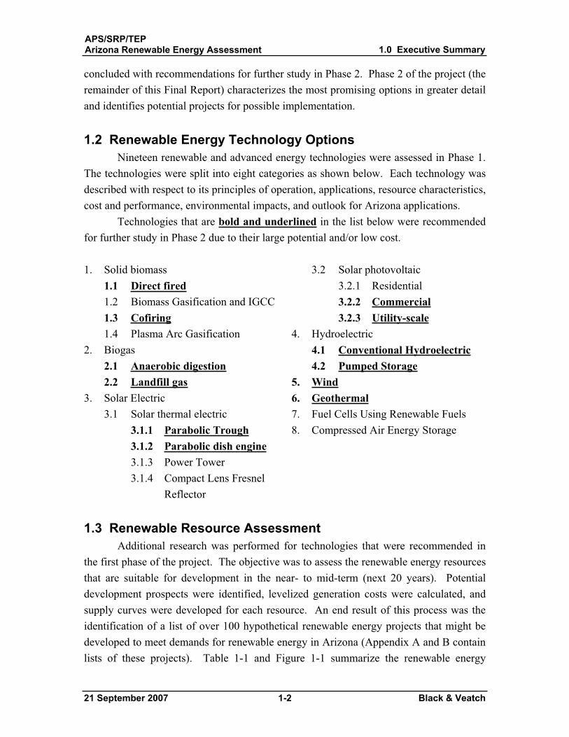
1.2 Renewable Energy Technology Options Nineteen renewable and advanced energy technologies were assessed in Phase 1.
The technologies were split into eight categories as shown below. Each technology was described with respect to its principles of operation, applications, resource characteristics, cost and performance, environmental impacts, and outlook for Arizona applications.
Technologies that are bold and underlined in the list below were recommended for further study in Phase 2 due to their large potential and/or low cost.
1. Solid biomass 1.1 Direct fired 1.2 Biomass Gasification and IGCC 1.3 Cofiring1.4 Plasma Arc Gasification
2. Biogas2.1 Anaerobic digestion 2.2 Landfill gas
3. Solar Electric 3.1 Solar thermal electric
3.1.1 Parabolic Trough3.1.2 Parabolic dish engine3.1.3 Power Tower 3.1.4 Compact Lens Fresnel
Reflector
3.2 Solar photovoltaic3.2.1 Residential3.2.2 Commercial3.2.3 Utility-scale
4. Hydroelectric4.1 Conventional Hydroelectric4.2 Pumped Storage
5. Wind6. Geothermal7. Fuel Cells Using Renewable Fuels 8. Compressed Air Energy Storage
1.3 Renewable Resource Assessment Additional research was performed for technologies that were recommended in
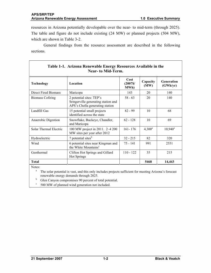
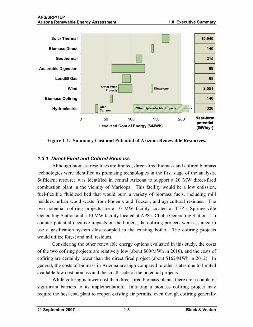
the first phase of the project. The objective was to assess the renewable energy resources that are suitable for development in the near- to mid-term (next 20 years). Potential development prospects were identified, levelized generation costs were calculated, and supply curves were developed for each resource. An end result of this process was the identification of a list of over 100 hypothetical renewable energy projects that might be developed to meet demands for renewable energy in Arizona (Appendix A and B contain lists of these projects). Table 1-1 and Figure 1-1 summarize the renewable energy
APS/SRP/TEPArizona Renewable Energy Assessment 1.0 Executive Summary
21 September 2007 1-2 Black & Veatch
resources in Arizona potentially developable over the near- to mid-term (through 2025). The table and figure do not include existing (24 MW) or planned projects (504 MW), which are shown in Table 3-2.
General findings from the resource assessment are described in the following sections.
Table 1-1. Arizona Renewable Energy Resources Available in the Near- to Mid-Term.
Technology Location Cost
(2007$/ MWh)
Capacity (MW)
Generation(GWh/yr)
Direct Fired Biomass Maricopa 143 20 140 Biomass Cofiring 2 potential sites: TEP’s
Sringerville generating station and APS’s Cholla generating station
58 - 63 20 140
Landfill Gas 15 potential small projects identified across the state
82 - 99 10 68
Anaerobic Digestion Snowflake, Buckeye, Chandler, and Maricopa
62 - 128 10 69
Solar Thermal Electric 100 MW project in 2011. 2–4 200 MW sites per year after 2012
161- 176 4,300a 10,940a
Hydroelectric 7 potential sitesb 32 - 215 82 320 Wind 6 potential sites near Kingman and
the White Mountainsc75 - 141 991 2551
Geothermal Clifton Hot Springs and Gillard Hot Springs
110 - 122 35 215
Total 5468 14,443 Notes:
a The solar potential is vast, and this only includes projects sufficient for meeting Arizona’s forecast renewable energy demands through 2025.
b Glen Canyon compromises 90 percent of total potential. c 500 MW of planned wind generation not included.
APS/SRP/TEPArizona Renewable Energy Assessment 1.0 Executive Summary
21 September 2007 1-3 Black & Veatch
0 50 100 150 200
Hydroelectric
Biomass Cofiring
Wind
Landfill Gas
Anaerobic Digestion
Geothermal
Biomass Direct
Solar Thermal
Levelized Cost of Energy ($/MWh)
320
140
2,551
68
69
215
140
10,940
Near-term potential (GWh/yr)
Glen Canyon
Other Hydroelectric Projects
KingstoneOther WindProjects
0 50 100 150 200
Hydroelectric
Biomass Cofiring
Wind
Landfill Gas
Anaerobic Digestion
Geothermal
Biomass Direct
Solar Thermal
Levelized Cost of Energy ($/MWh)
320
140
2,551
68
69
215
140
10,940
Near-term potential (GWh/yr)
Glen Canyon
Other Hydroelectric Projects
KingstoneOther WindProjects
Figure 1-1. Summary Cost and Potential of Arizona Renewable Resources.
1.3.1 Direct Fired and Cofired BiomassAlthough biomass resources are limited, direct-fired biomass and cofired biomass
technologies were identified as promising technologies in the first stage of the analysis. Sufficient resource was identified in central Arizona to support a 20 MW direct-fired combustion plant in the vicinity of Maricopa. This facility would be a low emission, fuel-flexible fluidized bed that would burn a variety of biomass fuels, including mill residues, urban wood waste from Phoenix and Tucson, and agricultural residues. The two potential cofiring projects are a 10 MW facility located at TEP’s Springerville Generating Station and a 10 MW facility located at APS’s Cholla Generating Station. To counter potential negative impacts on the boilers, the cofiring projects were assumed to use a gasification system close-coupled to the existing boiler. The cofiring projects would utilize forest and mill residues.
Considering the other renewable energy options evaluated in this study, the costs of the two cofiring projects are relatively low (about $60/MWh in 2010), and the costs of cofiring are certainly lower than the direct fired project (about $162/MWh in 2012). In general, the costs of biomass in Arizona are high compared to other states due to limited available low cost biomass and the small scale of the potential projects.
While cofiring is lower cost than direct fired biomass plants, there are a couple of significant barriers to its implementation. Initiating a biomass cofiring project may require the host coal plant to reopen existing air permits, even though cofiring generally
APS/SRP/TEPArizona Renewable Energy Assessment 1.0 Executive Summary
21 September 2007 1-4 Black & Veatch
reduces emissions. The risk and cost of reopening existing permits is not included in the cofiring cost estimate, but it may be a significant deterrent to cofiring projects. Further, electricity demand in Arizona is increasing faster than any other state (600 MW increase per year). Biomass cofiring converts capacity to a renewable source rather than adds capacity, and thus may be less attractive than new capacity additions.
If the cofiring projects face too many obstacles, an additional direct fired biomass facility could be developed in Northern Arizona in lieu of the cofiring projects.
1.3.2 Landfill Gas Black & Veatch utilized the Environmental Protection Agency Landfill Methane
Outreach Program (LMOP) database of landfills in Arizona to assess 25 potential sites. Black & Veatch attempted to contact each of the landfills to verify data and assess the suitability for power development. Based on this review, fifteen potential projects were identified, totaling 9.7 MW of capacity and 68 GWh of annual generation. This capacity is much smaller than what would be expected for similar sized landfills in other states due to Arizona’s dry climate. Most of these projects could be available by 2010 if development were prioritized. Projects costs vary, but most projects are projected to generate power for around $90/MWh.
The overall prospects for landfill gas generation are small. Landfill gas projects can take less time to develop than large solar or wind projects, so landfill gas may play a more significant role in the near term.
1.3.3 Anaerobic Digestion The utilization of biogas generated from anaerobic digestion of animal manure
was identified as a technically feasible option in the first stage of the analysis. Potential anaerobic digestion projects were identified based on large concentrations of livestock (swine, dairy, and poultry) operations within an area. Four anaerobic digestion projects were identified, ranging from 1.5 to 3.5 MW. The projects total 9.9 MW of capacity and 69 GWh of annual generation. The costs for the anaerobic digestion projects range from $70/MWh to $140/MWh (in 2010), largely dependent on project scale.
While this resource has a relatively limited generation potential, anaerobic digestion projects could be executed relatively quickly and with low levels of risk.
1.3.4 Solar Thermal Electric There is large potential for solar thermal development in Arizona. The review
focused on the only commercially proven technology: parabolic trough. Parabolic dish
APS/SRP/TEPArizona Renewable Energy Assessment 1.0 Executive Summary
21 September 2007 1-5 Black & Veatch
Stirling systems are promising, but unproven; their costs were assessed in a side scenario study (section 8).
The potential for solar thermal was characterized in a different manner than other technologies. Rather than being limited by resource availability, the technology is limited by equipment availability, development timelines, and ultimately economics. Due to supplier constraints, it was assumed that the first 100 MW trough plant in Arizona would not be completed until 2011. It is assumed that the near term supply chain constraints in the industry will be alleviated by 2013, and two to four 200 MW plants could be constructed per year thereafter. Generic projects were characterized in four areas of the state: Phoenix, Yuma, Stoval, and Tucson.
Unlike most other technologies evaluated for this study, it is expected that significant technical and cost advances will be realized for solar thermal trough plants. In addition, parabolic dish engine technology may also be deployed on a commercial level, and this technology could become competitive over the term of this study (through 2025).
The supply curve for solar thermal trough plants is relatively flat with the lowest cost projects generating power for about $160/MWh (hypothetical 2007 project, includes 30 percent investment tax credit). The flat supply curve means that a lot of solar thermal can be developed for about the same cost. This cost is substantially higher than non-solar resources profiled in this study. The potential supply of solar thermal potential is vast, and exceeds the near-term demands for renewable energy in Arizona.
1.3.5 Solar Photovoltaic As with solar thermal technologies, constraints on the deployment of solar
photovoltaic projects are not related to resource; the constraints are mainly capital costs and equipment availability. The review focused on deployment of larger photovoltaic systems (5-10 MW). Concentrating photovoltaic technology was also addressed as a possible future technology.
Even with significant cost reductions, costs for solar photovoltaic and concentrating photovoltaic projects are too high (greater than $240/MWh) to compete with the other renewable energy technologies surveyed. However, an advantage of solar photovoltaics is that smaller projects may be able to come online in the very near-term (2008 and 2009). As such, they are one of the few in-state technologies available to meet near-term renewable energy demand.
Alternative project and cost structures for solar PV projects are currently being refined, and they have the potential to substantially lower the “all-in” cost of energy from solar PV. Given the high capital costs for PV, any improvement in capital structure or
APS/SRP/TEPArizona Renewable Energy Assessment 1.0 Executive Summary
21 September 2007 1-6 Black & Veatch
financing costs has a relatively strong impact on the final levelized cost. These structures have not been modeled in this report.
1.3.6 Hydroelectric Seven hydroelectric projects were identified as potentially promising. The total
combined capacity of the seven projects identified is 81.8 MW, with an energy generation potential of 320 GWh/yr. A single project, adding generation at Glen Canyon dam, makes up about 90 percent of this total. The projects were identified based on government information, and details were difficult to verify. Of the seven projects, Glen Canyon, Tucson and Waddell are the only projects that could be reasonably located. Glen Canyon and Waddell have the most head and flow available compared to other sites. They also have existing hydropower installed and therefore show the most potential for further study. The Glen Canyon project is the lowest cost project of all the renewable energy projects surveyed for this study. It is forecast to cost about $50/MWh in 2015, the year it is projected to be available. The other hydroelectric projects are all projected to be much more expensive, at costs over $150/MWh in 2013, the first year they are projected to be available.
Drought conditions of recent years have reduced water resources throughout the Western US in recent years, including Lake Powell. Continued drought conditions may decrease the actual statewide hydroelectric potential.
1.3.7 Wind Power While the wind resource is generally less attractive in Arizona compared to
surrounding states, wind was identified as one of the more promising resources in the first phase of the study. To identify specific areas conducive to the development of a utility-scale wind energy projects, information was gathered on Arizona’s estimated wind resource, transmission infrastructure, environmental restrictions, and federal land areas. After reviewing many potential sites for constructability, transmission proximity, wind resource, and other constraints, six sites were chosen as the most promising for near-term development. While it is possible that other wind sites could be developed in Arizona, these sites are less attractive based on this analysis.
The total combined capacity of the six sites identified is 990 MW, with an energy generation potential of 2,550 GWh/yr. (The 500 MW of already planned wind projects are not included in this total). Costs for most projects are estimated to be about $75 to $100/MWh in 2010, which is the year when wind is first expected to be available. While the wind resources in Arizona are modest when judged against many other states, compared to other renewable energy options in Arizona, prospects for wind are good due
APS/SRP/TEPArizona Renewable Energy Assessment 1.0 Executive Summary
21 September 2007 1-7 Black & Veatch
to the relatively low cost. Arizona wind resources, however, are stronger in the winter when electricity demand is low, and weaker in the summer when demand is higher. Assessment of the seasonal value of energy (or avoided cost, more generally) was not included in the scope of this study.
1.3.8 Geothermal Geothermal was identified as a relatively unknown, but potentially promising
resource in the first phase of this study. The two known geothermal resources with the highest temperatures are located in the eastern part of the state: the Clifton Hot Springs and the Gillard Hot Springs projects. Interpretation of preliminary data suggests that resource temperatures may enable binary power generation.
Because the projects are still in their early exploratory state, there is not enough data available to accurately characterize the geothermal projects with a high degree of precision. Even identifying the potential project size is still speculative. For this reason, generic 20 and 15 MW projects were assumed. At best, these assumptions identify “place-holder” projects that must be further defined as more information about the true potential of each site is discovered. Because of their small-scale and long lead time (which places them after the assumed expiration of the production tax credit), costs for the two projects are relatively high ($149/MWh and $163/MWh in 2014). Nevertheless, this cost is still competitive with solar resources that are expected to be developed in the same timeframe.
1.4 Forecasted Renewable Energy Development Black & Veatch has developed a model to help utilities, states, and other entities
develop renewable energy plans. For the utilities represented in this study, Black & Veatch evaluated Arizona’s renewable energy development potential in light of increased demand for renewable energy stimulated, in part, by the Renewable Energy Standard. The model was then used to forecast renewable energy development in the state through 2025.
The model evaluates the total lifecycle cost of renewable energy projects, including capital and operating costs, performance, and transmission system interconnection. Projections are made for future changes in technology cost and performance based on Black & Veatch’s experience. By allowing the model to consider all possible renewable energy resources in Arizona, the study assesses the full potential of all renewable energy resources while accounting for the economics of developing those resources. The model does not include transmission system upgrades (other than interconnection costs) or system integration costs for intermittent resources (e.g. wind).
APS/SRP/TEPArizona Renewable Energy Assessment 1.0 Executive Summary
21 September 2007 1-8 Black & Veatch
The model also does not assess value (i.e., avoided cost) of the resource as determined by its degree of firmness or time of delivery (e.g. on-peak vs. off-peak). In selecting projects, utilities may consider these factors, which may result in a different order of resource/project development. Further, although long term transmission constraints have not been reviewed, a long term analysis should include a transmission development plan.
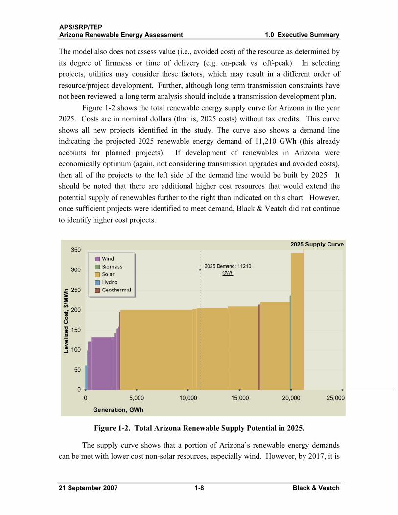
Figure 1-2 shows the total renewable energy supply curve for Arizona in the year 2025. Costs are in nominal dollars (that is, 2025 costs) without tax credits. This curve shows all new projects identified in the study. The curve also shows a demand line indicating the projected 2025 renewable energy demand of 11,210 GWh (this already accounts for planned projects). If development of renewables in Arizona were economically optimum (again, not considering transmission upgrades and avoided costs), then all of the projects to the left side of the demand line would be built by 2025. It should be noted that there are additional higher cost resources that would extend the potential supply of renewables further to the right than indicated on this chart. However, once sufficient projects were identified to meet demand, Black & Veatch did not continue to identify higher cost projects.
0 5,000 10,000 15,000 20,000 25,000
2025 Demand: 11210 GWh
0
50
100
150
200
250
300
350
Generation, GWh
Leve
lized
Cos
t, $/
MW
h
WindBiomass SolarHydroGeothermal
2025 Supply Curve
Figure 1-2. Total Arizona Renewable Supply Potential in 2025.
The supply curve shows that a portion of Arizona’s renewable energy demands can be met with lower cost non-solar resources, especially wind. However, by 2017, it is
APS/SRP/TEPArizona Renewable Energy Assessment 1.0 Executive Summary
21 September 2007 1-9 Black & Veatch
projected that lower cost non-solar resources will be exhausted and large-scale solar thermal plants will then be built at a rate of 200 to 400 MW per year through 2025. Other insights from the model include:
Non-solar resources limited – Arizona has a variety of renewable energy resources that could be developed; however, other than solar, these resources appear relatively limited. In the mid to near-term, developable potential for new biomass, geothermal, and hydroelectric projects combined could contribute about 952 GWh/yr, or 1 percent of the electricity that was generated in Arizona in 2005. Wind could contribute about 2.5 percent. With energy storage, solar could theoretically supply the entire electricity needs of the state. (Note that these totals exclude 825 GWh/yr of additional existing and already planned projects, most of which is wind).Non-solar resources important – Despite the relatively limited potential of wind, biomass, geothermal and hydroelectric resources, they serve an important role in forestalling the need to install expensive solar. However, the relatively limited potential of these resources compared to surrounding states may serve as a deterrent for large, out-of-state renewable energy project developers.Regional renewable energy markets – This study did not include an assessment of regional renewable energy supply and demand. Neighboring states, namely California, New Mexico, and Nevada, also have aggressive renewable energy standards. These states may have more economical renewable energy sources than Arizona (for example, Salton Sea geothermal resources and New Mexico wind); however, given their own aggressive in-state demands and transmission limitations, they may not be a dependable source for Arizona. While the importation of renewable energy may help to defer Arizona’s needs, it is not likely to fully satisfy them. Lowest cost resources – The most promising project opportunities from an economic perspective involve enhancements to existing facilities: adding a unit at the existing Glen Canyon hydroelectric project and biomass cofiring at the Cholla and Springerville coal plants. These projects are around $60/MWh or less.Solar about twice cost of other resources – Solar is the most expensive of the renewable resources profiled in this study. The lower cost solar resources (about $161-176/MWh in 2007) are about twice as expensive as the bulk of the non-solar resources (about $70-110/MWh in 2007). The base case model included only proven, fully commercial solar technologies such as solar
APS/SRP/TEPArizona Renewable Energy Assessment 1.0 Executive Summary
21 September 2007 1-10 Black & Veatch
photovoltaics and solar thermal trough. If forecasted technology improvements are realized, dish engine technologies have the potential to be cost competitive with conventional parabolic trough systems. Arizona’s reliance on solar is unique – Arizona appears unique in the U.S. in its dependence on in-state solar energy to meet its renewable energy demands. It is estimated that 65 percent of the Arizona renewable demand in 2025 will be met by solar. Generally speaking, other states in the Southwest U.S. will likely be less reliant on solar to meet their renewable energy requirements. This is because other states generally have a larger base of non-solar renewables that they can rely on for near-term needs. By comparison, Arizona’s non-solar resources are relatively limited. Solar technologies will play a key part of renewable’s future in Arizona. Consideration of avoided costs is important and necessary – This project did not assess the differential value (i.e., avoided cost) of renewable resources.Avoided cost is typically determined by assessing a resource’s capacity value (based on degree of “firmness” at the time of a utility’s system peak demand) and its energy value (based on time of delivery). In selecting projects to develop or procure, utilities may consider these factors, which may result in a different order of resource/project development than shown in the supply curves in this report. This is important when comparing resources such as wind and solar. For example, wind energy projects only provide fractional capacity value (often estimated at 20 percent of the nameplate capacity) and are more likely to offset low cost energy resources during the winter and spring. Solar resources can readily provide firm capacity with gas hybridization or thermal storage. Further, solar is generally coincident with times of higher capacity needs. There are numerous methods to calculate avoided cost, and costs are specific to individual utility systems.
1.5 Assessment of Key Risk Factors Black & Veatch analyzed some of the risk factors of interest to utilities in Arizona
to determine how sensitive the supply curve results would be to changing situations. These factors include tax credit changes, implementation of advanced solar technologies, delayed technical advances, escalating construction costs, manufacturing/supply chain constraints, near term performance learning curve, and competition for limited resources.
APS/SRP/TEPArizona Renewable Energy Assessment 1.0 Executive Summary
21 September 2007 1-11 Black & Veatch
1.5.1 Tax Credit Changes Most renewable resources benefit from either production tax credits (PTCs) or
investment tax credits (ITCs). The base case model assumed tax credits expire in 2012. In the long term, whether tax credits expire in 2008 or 2012 has little impact on the cumulative average cost of meeting renewable energy demand in Arizona (less than 1 percent by 2025). This is because many of the most expensive, large solar projects would likely be built after 2012. If tax credits never expire, the impact is a significant reduction in cumulative portfolio costs (25 percent reduction).
1.5.2 Advanced Solar Technologies There are pre-commercial advanced solar technologies that may reduce the cost of
solar energy. Two of these technologies include concentrating solar photovoltaic (CPV) and parabolic dish engine. These technologies were not included in the base case model, but were modeled in a sensitivity analysis. Based on Black & Veatch’s assumptions, technology advancements in CPV will not make that technology competitive with conventional solar parabolic trough technologies for utility scale applications. However, there does appear to be potential for dish engine technologies to become competitive with solar trough technology.
1.5.3 Delayed Technical Advances Advances are expected in wind and solar technologies, resulting in lower costs
and higher capacity factors. However, there is a risk that such advancement may be delayed or not realized, and this was investigated in a sensitivity analysis. When technology advances were delayed, wind and solar thermal projects had lower capacity factors compared to the base case, which required development of more projects to meet the same demand. Because of lack of advancement, solar projects, particularly in the later years, are higher cost than the base case. The reduced technical advances will make levelized costs for wind and solar higher, which will make other technologies (biomass and geothermal) comparatively more attractive in early years. The cumulative effect on the total renewable energy cost will likely be an increase of 15 to 20 percent by 2025.
1.5.4 Escalating Construction Costs The model base case has a capital cost escalation of 2.5 percent per year, which is
meant to track close to general inflation. There is a risk that construction costs will escalate at a higher rate, depending on future markets for materials and labor. A sensitivity analysis was performed assuming 5 percent escalation. The results are pronounced. At year 2025, levelized costs are about 37 percent higher than the base case.
APS/SRP/TEPArizona Renewable Energy Assessment 1.0 Executive Summary
21 September 2007 1-12 Black & Veatch
1.5.5 Manufacturing and Supply Chain Constraints Manufacturing and supply chain constraints were assumed in the model. The
projects most likely to be impacted by such constraints are solar and wind. For wind projects, there is currently a delay of up to two years between turbine order and turbine delivery because demand is greater than manufacturing capability. The wind projects identified for this project are assumed to be available to come online between 2010 and 2013. If there are additional constraints in the turbine supply chain, then it is likely that renewable energy demand would not be met in some years with in-state resources.
Solar projects were also modeled with manufacturing constraints in mind. Due to these constraints, it has been assumed that the first 100 MW trough plant in Arizona could not be completed until 2011. It is assumed that the near-term supply chain constraints in the industry will be alleviated by 2013, and two to four 200 MW plants could be constructed per year thereafter if deemed economical
1.5.6 Near-Term Performance Learning Curve / Project Failure In the near-term, projects may under-deliver renewable energy as they gain
experience during the initial operational and development learning period. Projects may also fail outright, and not supply any renewable energy. From a supply curve standpoint, contract failure shifts the supply curve to the left. When a project fails, its generation is removed from the supply curve, while all projects to the right (more expensive projects) shift left to fill in the space. As lower-priced projects fail, utilities will be forced to contract with more expensive renewable projects to procure the necessary amount of energy.
1.5.7 Competition for Limited Renewable Resources As more and more renewable energy projects are developed, there will be fewer
renewable resources to utilize in the future. There is a risk that utility competition for limited renewable resources will increase prices. This is particularly true in supply-constrained markets. For Arizona utilities, it is possible that renewable energy developers may set energy prices as high as possible while still beating the marginal cost of competing energy supplies. This would increase the total renewable energy cost, but it is uncertain to what extent.
APS/SRP/TEPArizona Renewable Energy Assessment 2.0 Introduction
21 September 2007 2-1 Black & Veatch
2.0 Introduction
Black & Veatch Corporation has prepared this study of renewable energy for the three largest utilities in Arizona: Arizona Public Service Company, Salt River Project, and Tucson Electric Power Company (APS/SRP/TEP). The purpose of this report is to assess the prospects for significant renewable energy development in Arizona. The scope of the study is limited to Arizona projects that would export power to the grid (that is, not distributed generation projects).
This study includes a review of the current status of renewable energy in Arizona, characterization of renewable power generation technologies, assessment of Arizona’s renewable resources, and an assessment of key risk factors.
2.1 Background In response to increasing public interest in clean energy sources, concerns about
energy security, and the environmental impacts of fossil fuels, numerous states have encouraged development of renewable energy sources. Renewable energy standards have been a popular mechanism used by other states and countries to mandate a certain percentage of electricity be generated from renewable energy resources.
Electricity in Arizona is largely produced from traditional natural gas, coal, and nuclear resources. Hydroelectric contributes about 6 percent, while non-hydro renewable resources are currently very small (0.07 percent). To stimulate development of renewables, Arizona was one of the earlier states to adopt a renewable energy standard. Arizona enacted its original Environmental Portfolio Standard (EPS) in March of 2001. The EPS required that investor owned utilities provide 1.1 percent of their power from renewables by 2007.
In November 2006, the Arizona Corporation Commission adopted final rules to substantially increase Arizona’s Renewable Energy Standard (RES) such that some utilities would be required to obtain 15 percent of their energy from renewable resources by 2025. Such a standard places Arizona among the most aggressive in the nation. In addition, Arizona is surrounded by other states in the Southwest (California, Nevada, and New Mexico) that also have strong renewable energy standards. The combined effect of these standards is to substantially increase the demand for renewable energy in the region.
2.2 Objective The objective of this report is to assess the full potential of all Arizona renewable
energy resources while accounting for the economic variables of developing those
APS/SRP/TEPArizona Renewable Energy Assessment 2.0 Introduction
21 September 2007 2-2 Black & Veatch
resources. Large scale renewable energy development will be necessary to meet the renewable mandates set forth in the Southwest. Although Arizona is well known for its solar resources, solar is the most expensive renewable energy resource. By comparison, Arizona is thought by many to have relatively limited opportunities for lower cost renewables, including wind, biomass, geothermal and hydroelectric. This study assesses the relative potential of all resources and forecasts which are most likely to be developed over the next 20 years.
2.3 Approach Black & Veatch has developed an objective methodology to assess renewable
energy potential based on sound utility generation planning fundamentals and the specific challenges inherent to analyzing renewable energy generation technologies. This study was undertaken in two phases. This final report is a comprehensive account of both. An Interim Report covered Phase 1. It described the current status of renewable energy in Arizona, characterized renewable power generation technologies and the general potential of the different resources, and reviewed available financial incentives for renewable energy. The Interim Report (Section 3, 4 and 6 of this Final Report) reviewed a broad range of renewable energy technologies and concluded with recommendations for further study in Phase 2. Phase 2 of the project (the remainder of this Final Report) characterizes the most promising options in greater detail and identifies potential projects for possible implementation.
This study began with an assessment of renewable energy generation technologies to identify the most promising technologies for Arizona. The following technologies were initially identified as potentially promising:
Wind Solar Thermal (trough) Solar Thermal (dish) Solar Photovoltaics Direct Biomass Combustion Cofired Biomass Anaerobic Digestion Landfill Gas HydroelectricGeothermal
Following identification of the most promising technologies, a resource assessment was performed to quantify the near-term developable potential of the promising renewable resources. In some cases, the assessment included new primary
APS/SRP/TEPArizona Renewable Energy Assessment 2.0 Introduction
21 September 2007 2-3 Black & Veatch
research and initial siting activities to collect renewable energy resource data. This information was used to determine the size of the resources, geographic distribution, and technical feasibility of utilization. An end result of this process was the identification of a list of over 100 hypothetical renewable energy projects that might be developed to meet demands for renewable energy.
Following the resource assessment, the total lifecycle costs were calculated for each renewable energy project. Costs included capital and operating costs, performance, transmission system interconnection, and financial incentives. Transmission costs, which can be significant, have not been included at this stage of the analysis. Projections were also made for future changes in technology cost and performance based on Black & Veatch’s experience in the field. Resource estimates were combined with technology characteristics to develop a set of economic supply curves showing the renewable energy available (MWh) at different levelized costs ($/MWh). The supply curves for the individual renewable energy technologies were then combined to generate statewide renewable energy supply curves. The supply curves can be used to identify a hypothetical least-cost set of renewable energy projects through 2025.
Once the base model was established, it was used to test the model results against various key risk factors.
2.4 Report Organization Following this Introduction, this report is organized into the following sections:
Section 3 – Renewable Energy Overview: This section provides an overview of renewable energy including the historical development of renewables in the US followed by the status of renewable energy in Arizona.Section 4 – Assessment of Renewable Energy Technology Options: This section reviews the general characteristics and costs of renewable energy technology options for Arizona. The section concludes with a short list of technologies recommended for further study. Section 5 – Renewable Resource Assessment: This section summarizes the renewable energy resources of Arizona that are suitable for development in the near- to mid-term (next 20 years). Potential development prospects are identified, levelized generation costs are calculated, and a set of supply curves is developed. Section 6 – Renewable Energy Financial Incentives: This section describes the existing and proposed incentives that are available to new renewable energy facilities.
APS/SRP/TEPArizona Renewable Energy Assessment 2.0 Introduction
21 September 2007 2-4 Black & Veatch
Section 7 – Renewable Energy Development Model: This section summarizes the supply curve model. The model is described, assumptions are outlined, and key results are presented. Section 8 – Assessment of Key Risk Factors: Black & Veatch analyzed some of the risk factors of interest to utilities in Arizona to determine how sensitive the supply curve results would be to changing situations. These factors include changes in tax law, delayed technical advances, escalating construction costs, manufacturing/supply chain constraints, near term performance learning curve, and competition for limited resources.
APS/SRP/TEPArizona Renewable Energy Assessment 3.0 Renewable Energy Overview
21 September 2007 3-1 Black & Veatch
3.0 Renewable Energy Overview
This section provides an overview of renewable energy including the historical development of renewables in the US followed by the status of renewable energy in Arizona.
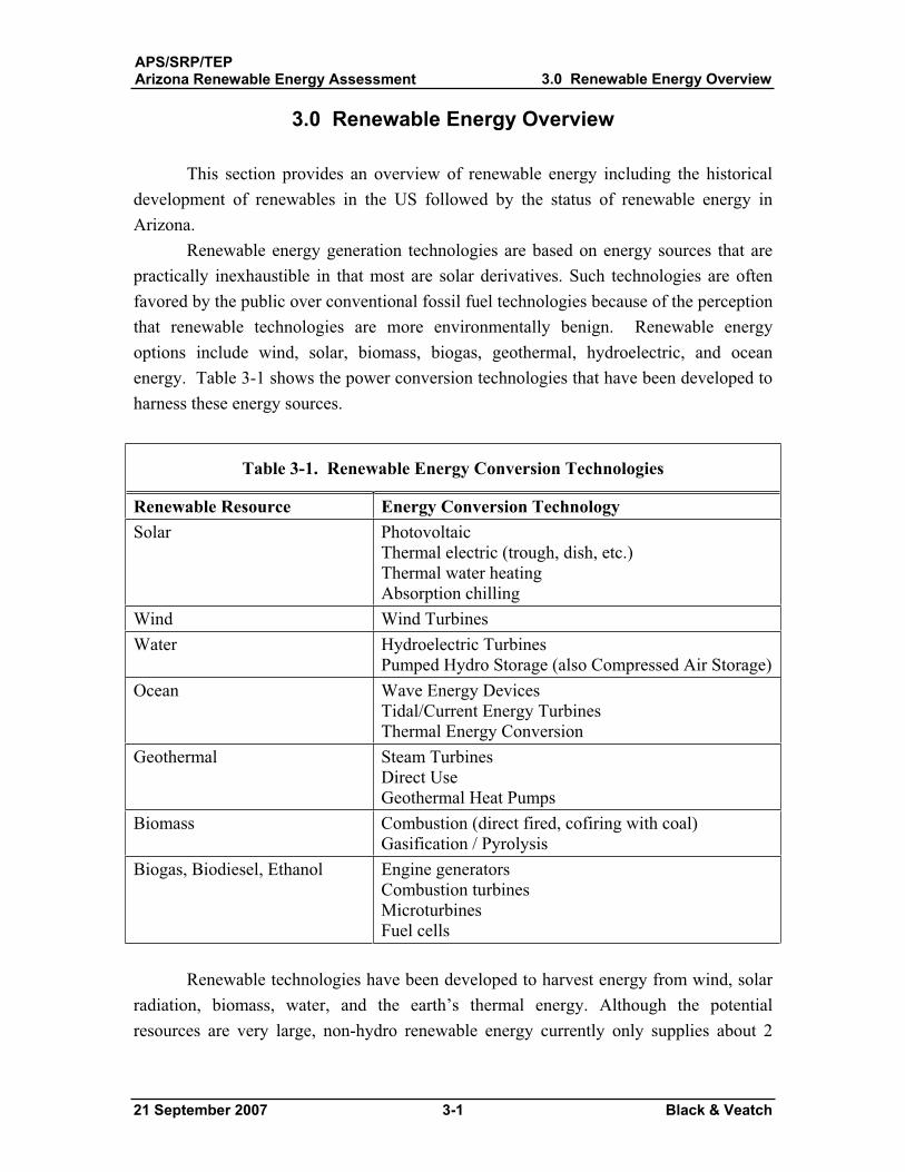
Renewable energy generation technologies are based on energy sources that are practically inexhaustible in that most are solar derivatives. Such technologies are often favored by the public over conventional fossil fuel technologies because of the perception that renewable technologies are more environmentally benign. Renewable energy options include wind, solar, biomass, biogas, geothermal, hydroelectric, and ocean energy. Table 3-1 shows the power conversion technologies that have been developed to harness these energy sources.
Table 3-1. Renewable Energy Conversion Technologies
Renewable Resource Energy Conversion Technology Solar Photovoltaic
Thermal electric (trough, dish, etc.) Thermal water heating Absorption chilling
Wind Wind Turbines Water Hydroelectric Turbines
Pumped Hydro Storage (also Compressed Air Storage)Ocean Wave Energy Devices
Tidal/Current Energy Turbines Thermal Energy Conversion
Geothermal Steam Turbines Direct Use Geothermal Heat Pumps
Biomass Combustion (direct fired, cofiring with coal) Gasification / Pyrolysis
Biogas, Biodiesel, Ethanol Engine generators Combustion turbines Microturbines Fuel cells
Renewable technologies have been developed to harvest energy from wind, solar radiation, biomass, water, and the earth’s thermal energy. Although the potential resources are very large, non-hydro renewable energy currently only supplies about 2
APS/SRP/TEPArizona Renewable Energy Assessment 3.0 Renewable Energy Overview
21 September 2007 3-2 Black & Veatch
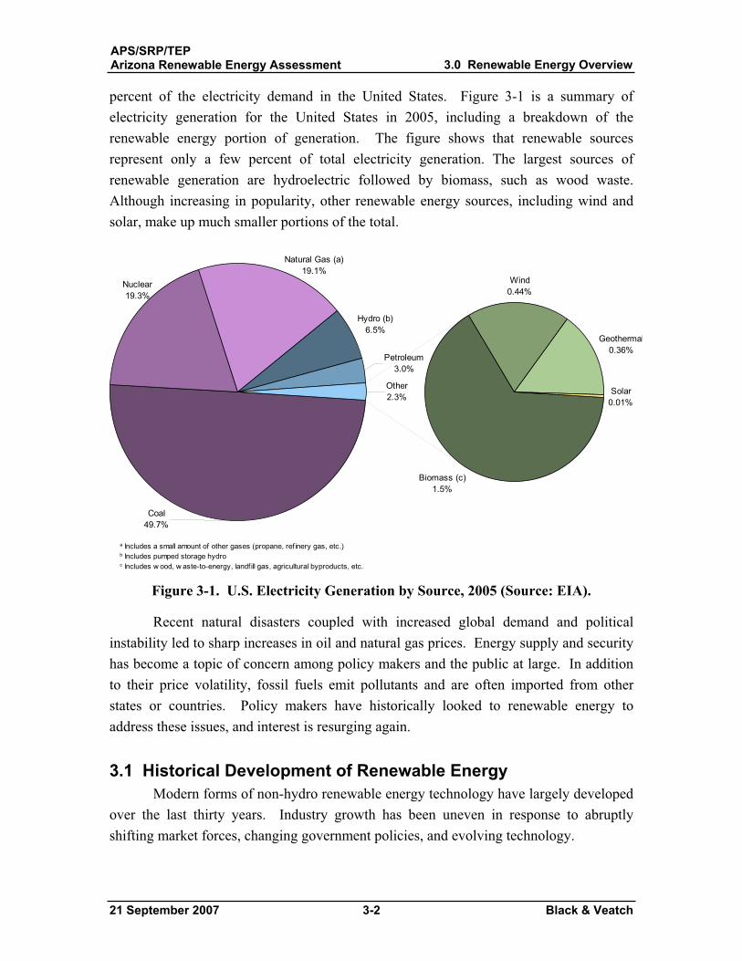
percent of the electricity demand in the United States. Figure 3-1 is a summary of electricity generation for the United States in 2005, including a breakdown of the renewable energy portion of generation. The figure shows that renewable sources represent only a few percent of total electricity generation. The largest sources of renewable generation are hydroelectric followed by biomass, such as wood waste. Although increasing in popularity, other renewable energy sources, including wind and solar, make up much smaller portions of the total.
Hydro (b)6.5%
Petroleum3.0%
Biomass (c) 1.5%
Other2.3%
Geothermal0.36%
Wind0.44%
Solar0.01%
Natural Gas (a)19.1%
Coal49.7%
Nuclear19.3%
a Includes a small amount of other gases (propane, ref inery gas, etc.)b Includes pumped storage hydroc Includes w ood, w aste-to-energy, landfill gas, agricultural byproducts, etc.
Figure 3-1. U.S. Electricity Generation by Source, 2005 (Source: EIA).
Recent natural disasters coupled with increased global demand and political instability led to sharp increases in oil and natural gas prices. Energy supply and security has become a topic of concern among policy makers and the public at large. In addition to their price volatility, fossil fuels emit pollutants and are often imported from other states or countries. Policy makers have historically looked to renewable energy to address these issues, and interest is resurging again.
3.1 Historical Development of Renewable Energy Modern forms of non-hydro renewable energy technology have largely developed
over the last thirty years. Industry growth has been uneven in response to abruptly shifting market forces, changing government policies, and evolving technology.
APS/SRP/TEPArizona Renewable Energy Assessment 3.0 Renewable Energy Overview
21 September 2007 3-3 Black & Veatch
3.1.1 1978-1991: PURPA and Standard Offer Contracts The modern era of renewable energy arose from the initial oil shortages of the
1970s. In 1978, the federal government passed the Public Utilities Regulatory Policy Act, which stimulated widespread development of renewable energy projects. Under PURPA, many biomass, wind, and geothermal plants came online and were allowed to sell excess power to the utility at an avoided cost or other negotiated rate. Some of these costs/rates, particularly in California, were tied to high forecasts of future fossil prices. The generous PURPA contracts combined with other financial incentives allowed California to lead the world in development of biomass, geothermal, wind and solar technologies. Ultimately, PURPA spurred the development of the independent power producer (IPP) industry. IPPs currently dominate ownership of renewable energy plants.
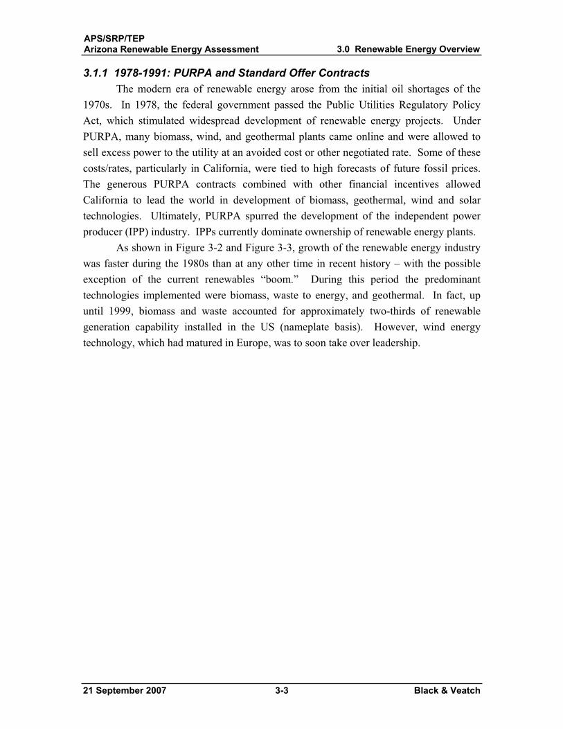
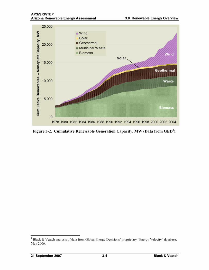
As shown in Figure 3-2 and Figure 3-3, growth of the renewable energy industry was faster during the 1980s than at any other time in recent history – with the possible exception of the current renewables “boom.” During this period the predominant technologies implemented were biomass, waste to energy, and geothermal. In fact, up until 1999, biomass and waste accounted for approximately two-thirds of renewable generation capability installed in the US (nameplate basis). However, wind energy technology, which had matured in Europe, was to soon take over leadership.
APS/SRP/TEPArizona Renewable Energy Assessment 3.0 Renewable Energy Overview
21 September 2007 3-4 Black & Veatch
0
5,000
10,000
15,000
20,000
25,000
1978 1980 1982 1984 1986 1988 1990 1992 1994 1996 1998 2000 2002 2004
Cum
ulat
ive
Rene
wab
les
-- Na
mep
late
Cap
acity
, MW Wind
SolarGeothermalMunicipal WasteBiomass
Biomass
Waste
Geothermal
WindSolar
Figure 3-2. Cumulative Renewable Generation Capacity, MW (Data from GED1).
1 Black & Veatch analysis of data from Global Energy Decisions’ proprietary “Energy Velocity” database, May 2006.
APS/SRP/TEPArizona Renewable Energy Assessment 3.0 Renewable Energy Overview
21 September 2007 3-5 Black & Veatch
0
500
1,000
1,500
2,000
2,500
1978 1980 1982 1984 1986 1988 1990 1992 1994 1996 1998 2000 2002 2004
Annu
al A
dditi
ons
-- Na
mep
late
Cap
acity
, MW
WindSolarGeothermalMunicipal WasteBiomass
WindGeothermalSolar
Biomass
Waste
Figure 3-3. U.S. Annual Capacity Additions, MW (Data from GED).
3.1.2 1992-2004: The PTC and RPS Era As the influence of PURPA waned with lower electricity costs in the 1990s, a
new round of renewable energy development, mostly wind, was spurred by the Production Tax Credit (PTC) enacted in 1992. Despite the new incentive, development in the early 1990s was at a much slower pace than during the 1980s.
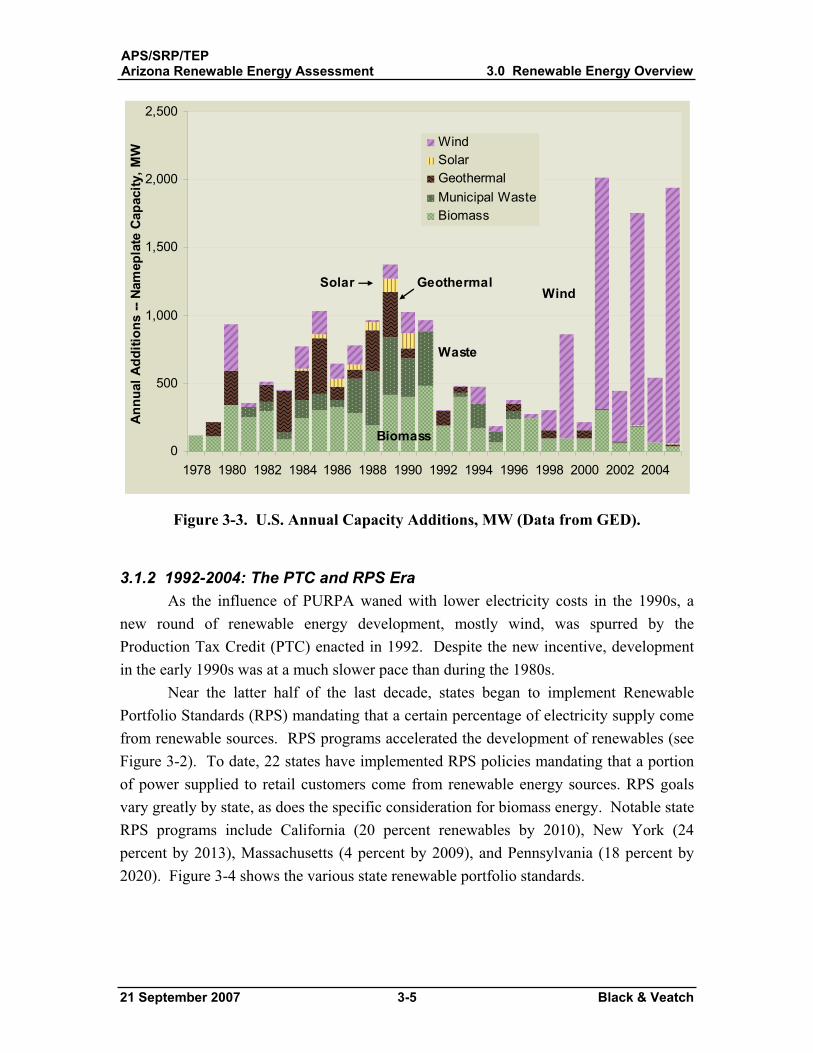
Near the latter half of the last decade, states began to implement Renewable Portfolio Standards (RPS) mandating that a certain percentage of electricity supply come from renewable sources. RPS programs accelerated the development of renewables (see Figure 3-2). To date, 22 states have implemented RPS policies mandating that a portion of power supplied to retail customers come from renewable energy sources. RPS goals vary greatly by state, as does the specific consideration for biomass energy. Notable state RPS programs include California (20 percent renewables by 2010), New York (24 percent by 2013), Massachusetts (4 percent by 2009), and Pennsylvania (18 percent by 2020). Figure 3-4 shows the various state renewable portfolio standards.
APS/SRP/TEPArizona Renewable Energy Assessment 3.0 Renewable Energy Overview
21 September 2007 3-6 Black & Veatch
MA: 4%MA: 4%By 2009,By 2009,+1%/yr+1%/yrafterafter
States with RPS Requirements
States with RPS Goals
CA: 20%CA: 20%by 2010by 2010
NV: 20%NV: 20%by 2015,by 2015,5% Solar5% Solar
AZ: 15%AZ: 15%By 2025By 2025 NM: 20%NM: 20%
by 2020by 2020
TX: 5,880 MW (5%)TX: 5,880 MW (5%)by 2015by 2015
MN: 25% MN: 25% by 2025 by 2025
(Xcel(Xcel30%)30%) WI: 10%WI: 10%
by 2015by 2015
IA: 105 MWIA: 105 MWIL Goal:IL Goal:
8%8%By 2013By 2013
HI: 20%HI: 20%By 2020By 2020
NJ: 22.5%NJ: 22.5%By 2021By 2021
CT: 10%CT: 10%By 2010By 2010
ME: 30%ME: 30%
MD: 7.5%MD: 7.5%By 2019By 2019
RI: 16%RI: 16%By 2020By 2020
CO: 20%CO: 20%by 2020by 20204% Solar4% Solar
NY: 24%NY: 24%by 2013by 2013
PA: 8/10% PA: 8/10% Tier I/II Tier I/II by 2020by 2020
DC: 11%DC: 11%By 2022By 2022
VT Goal: All NewVT Goal: All NewGen, 10% capGen, 10% capMT: 15%MT: 15%
By 2015By 2015
DE: 10%DE: 10%By 2019By 2019
WA: 15%WA: 15%By 2020By 2020
NH: 16% new NH: 16% new Gen By 2025Gen By 2025
VA Goal:VA Goal:12%12%
By 2022By 2022
Figure 3-4. State Renewable Portfolio Standards (as of May 2007).
Based on developments in Europe, wind energy technology had also greatly improved from the designs of the 1980s. Wind benefited greatly from the combination of preferential PTC treatment, RPS programs, and improved technology. Since 1999, about 90 percent of all new renewable energy development has been wind (nameplate capacity basis). Prior to 1999, wind comprised about 10 percent of total renewables additions.
3.1.3 2005: Energy Policy Act In the past year, changes in federal tax policy and a surge in demand for
renewable energy have caused a new era in renewable energy development.Federal involvement in the energy industry has traditionally been limited due to
strong state regulation; however, the federal government is increasing its role, especially with respect to renewable energy. Recently, the government has significantly expanded tax and other incentives for renewable energy developers through the Energy Policy Act of 2005 (EPAct). The federal government has traditionally funded renewable research and development through the Department of Energy, and President Bush’s recent state of the Union address called for more investment and spending on renewables.
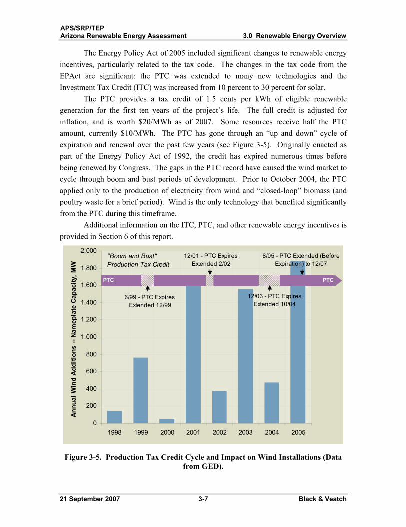
APS/SRP/TEPArizona Renewable Energy Assessment 3.0 Renewable Energy Overview
21 September 2007 3-7 Black & Veatch
The Energy Policy Act of 2005 included significant changes to renewable energy incentives, particularly related to the tax code. The changes in the tax code from the EPAct are significant: the PTC was extended to many new technologies and the Investment Tax Credit (ITC) was increased from 10 percent to 30 percent for solar.
The PTC provides a tax credit of 1.5 cents per kWh of eligible renewable generation for the first ten years of the project’s life. The full credit is adjusted for inflation, and is worth $20/MWh as of 2007. Some resources receive half the PTC amount, currently $10/MWh. The PTC has gone through an “up and down” cycle of expiration and renewal over the past few years (see Figure 3-5). Originally enacted as part of the Energy Policy Act of 1992, the credit has expired numerous times before being renewed by Congress. The gaps in the PTC record have caused the wind market to cycle through boom and bust periods of development. Prior to October 2004, the PTC applied only to the production of electricity from wind and “closed-loop” biomass (and poultry waste for a brief period). Wind is the only technology that benefited significantly from the PTC during this timeframe.
Additional information on the ITC, PTC, and other renewable energy incentives is provided in Section 6 of this report.
0
200
400
600
800
1,000
1,200
1,400
1,600
1,800
2,000
1998 1999 2000 2001 2002 2003 2004 2005
Annu
al W
ind
Addi
tions
-- N
amep
late
Cap
acity
, MW
6/99 - PTC ExpiresExtended 12/99
PTC PTC
12/01 - PTC ExpiresExtended 2/02
12/03 - PTC ExpiresExtended 10/04
8/05 - PTC Extended (Before Expiration) to 12/07
"Boom and Bust" Production Tax Credit
Figure 3-5. Production Tax Credit Cycle and Impact on Wind Installations (Data from GED).
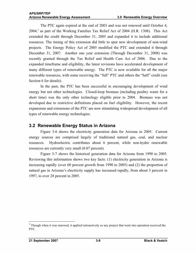
APS/SRP/TEPArizona Renewable Energy Assessment 3.0 Renewable Energy Overview
21 September 2007 3-8 Black & Veatch
The PTC again expired at the end of 2003 and was not renewed until October 4, 2004,2 as part of the Working Families Tax Relief Act of 2004 (H.R. 1308). This Act extended the credit through December 31, 2005 and expanded it to include additional resources. The timing of this extension did little to spur new development of non-wind projects. The Energy Policy Act of 2005 modified the PTC and extended it through December 31, 2007. Another one year extension (Through December 31, 2008) was recently granted through the Tax Relief and Health Care Act of 2006. Due to the expanded timeframe and eligibility, the latest revisions have accelerated development of many different types of renewable energy. The PTC is now available for all the major renewable resources, with some receiving the “full” PTC and others the “half” credit (see Section 6 for details).
In the past, the PTC has been successful in encouraging development of wind energy but not other technologies. Closed-loop biomass (including poultry waste for a short time) was the only other technology eligible prior to 2004. Biomass was not developed due to restrictive definitions placed on fuel eligibility. However, the recent expansions and extensions of the PTC are now stimulating widespread development of all types of renewable energy technologies.
3.2 Renewable Energy Status in Arizona Figure 3-6 shows the electricity generation data for Arizona in 2005. Current
energy sources are comprised largely of traditional natural gas, coal, and nuclear resources. Hydroelectric contributes about 6 percent, while non-hydro renewable resources are currently very small (0.07 percent).
Figure 3-7 shows the historical generation data for Arizona from 1990 to 2005. Reviewing this information shows two key facts: (1) electricity generation in Arizona is increasing rapidly (over 60 percent growth from 1990 to 2005) and (2) the proportion of natural gas in Arizona’s electricity supply has increased rapidly, from about 3 percent in 1997, to over 28 percent in 2005.
2 Though when it was renewed, it applied retroactively so any project that went into operation received the PTC.
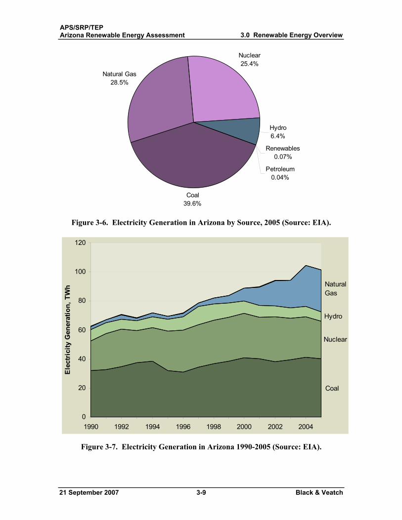
APS/SRP/TEPArizona Renewable Energy Assessment 3.0 Renewable Energy Overview
21 September 2007 3-9 Black & Veatch
Coal39.6%
Natural Gas28.5%
Nuclear25.4%
Hydro6.4%
Petroleum0.04%
Renewables0.07%
Figure 3-6. Electricity Generation in Arizona by Source, 2005 (Source: EIA).
Coal
Nuclear
Hydro
NaturalGas
0
20
40
60
80
100
120
1990 1992 1994 1996 1998 2000 2002 2004
Elec
trici
ty G
ener
atio
n, T
Wh
Figure 3-7. Electricity Generation in Arizona 1990-2005 (Source: EIA).
APS/SRP/TEPArizona Renewable Energy Assessment 3.0 Renewable Energy Overview
21 September 2007 3-10 Black & Veatch
3.2.1 Existing and Announced Renewable Energy Projects Although renewables currently only comprise a small fraction of the electricity in
Arizona, this will likely change in the near future. Table 3-2 shows existing and announced renewable energy projects (excluding large hydroelectric projects). There are about 24 MW of renewable energy projects currently operating in Arizona, including 12 MW of biomass, 0.8 MW hydroelectric, and the remainder solar (11 MW). In addition, there are over 500 MW of projects in various stages of development throughout the state. The vast majority of these projects are based on wind resources, although there is a 20 MW biomass project under construction in eastern Arizona.
3.2.2 Arizona Renewable Energy Standard3
Arizona was one of the earlier states to adopt a renewable portfolio standard mandating that utilities source a portion of their energy from renewable energy sources. Arizona enacted its original Environmental Portfolio Standard (EPS) in March of 2001. The EPS required that investor owned utilities provide 1.1 percent of their power from renewables by 2007. The standard began with a requirement of 0.2 percent in 2002, increasing by 0.2 percent annually. Solar electric was to make up 50 percent of the standard in 2001, increasing to 60 percent for 2004 through 2012. Although the EPS was largely responsible for several of the projects identified in the previous section, many felt that the mandate needed to be revised.
After much deliberation, on November 14th, 2006 the Arizona Corporation Commission (ACC) adopted a new Renewable Energy Standard (RES) that requires utilities to meet higher targets for renewable energy sources. The requirement begins at 1.25 percent renewables in 2006 and stair-steps up to 15 percent renewable energy production by 2025 (see Table 3-3). A certain portion of the RES must be met with distributed renewable energy generation sources, such as small solar and wind. This is also known as a set-aside. The set-asides begin at 5 percent of the standard in 2007 and rise to 30 percent of the renewable standard percentage in 2012 and thereafter. At the full 15 percent standard in 2025, the set-aside would be 30 percent of total renewable requirement of 15 percent, or 4.5 percent of total electricity generation (10.5 is non-distributed resources). One half of the distributed resource requirement must come from residential installations, the other half must be from non-residential, non-utility applications. The purpose of the set-aside is to encourage renewable energy production from distributed sources such as small solar or wind equipment located on or near ratepayer property instead of larger, centralized renewable power plants.
3 Source: ACC Decision No. 69127 (AAC R14-2-1801 et seq.), available at: http://www.cc.state.az.us/utility/electric/res.pdf, accessed January 2007.
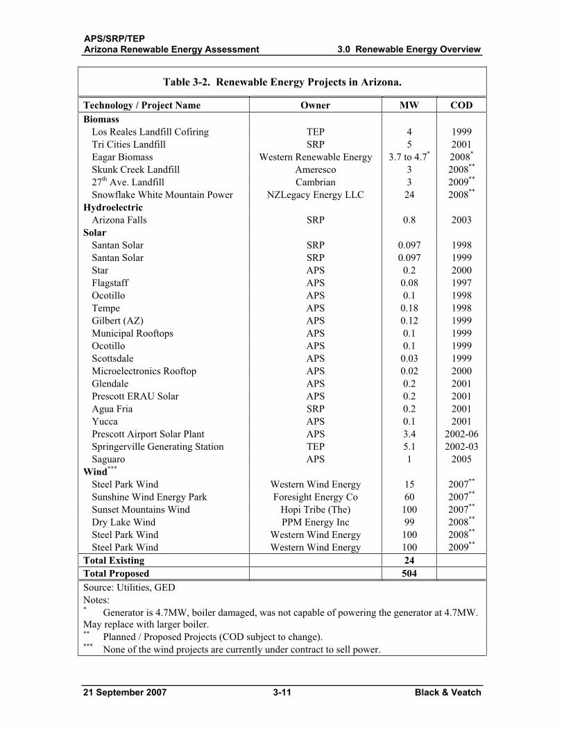
APS/SRP/TEPArizona Renewable Energy Assessment 3.0 Renewable Energy Overview
21 September 2007 3-11 Black & Veatch
Table 3-2. Renewable Energy Projects in Arizona.
Technology / Project Name Owner MW COD Biomass
Los Reales Landfill Cofiring TEP 4 1999 Tri Cities Landfill SRP 5 2001 Eagar Biomass Western Renewable Energy 3.7 to 4.7* 2008*
Skunk Creek Landfill Ameresco 3 2008**
27th Ave. Landfill Cambrian 3 2009**
Snowflake White Mountain Power NZLegacy Energy LLC 24 2008**
Hydroelectric Arizona Falls SRP 0.8 2003
Solar Santan Solar SRP 0.097 1998 Santan Solar SRP 0.097 1999 Star APS 0.2 2000 Flagstaff APS 0.08 1997 Ocotillo APS 0.1 1998 Tempe APS 0.18 1998 Gilbert (AZ) APS 0.12 1999 Municipal Rooftops APS 0.1 1999 Ocotillo APS 0.1 1999 Scottsdale APS 0.03 1999 Microelectronics Rooftop APS 0.02 2000 Glendale APS 0.2 2001 Prescott ERAU Solar APS 0.2 2001 Agua Fria SRP 0.2 2001 Yucca APS 0.1 2001 Prescott Airport Solar Plant APS 3.4 2002-06 Springerville Generating Station TEP 5.1 2002-03 Saguaro APS 1 2005
Wind*** Steel Park Wind Western Wind Energy 15 2007**
Sunshine Wind Energy Park Foresight Energy Co 60 2007**
Sunset Mountains Wind Hopi Tribe (The) 100 2007**
Dry Lake Wind PPM Energy Inc 99 2008**
Steel Park Wind Western Wind Energy 100 2008**
Steel Park Wind Western Wind Energy 100 2009**
Total Existing 24 Total Proposed 504 Source: Utilities, GED Notes:* Generator is 4.7MW, boiler damaged, was not capable of powering the generator at 4.7MW. May replace with larger boiler. ** Planned / Proposed Projects (COD subject to change). *** None of the wind projects are currently under contract to sell power.
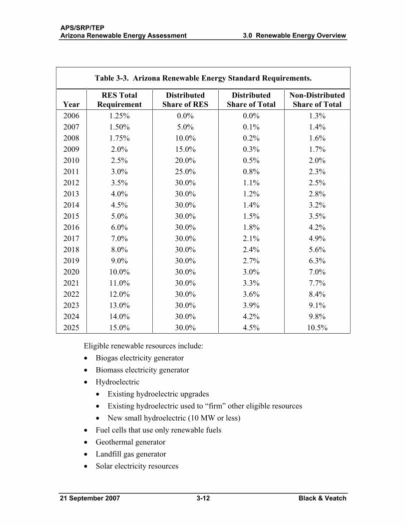
APS/SRP/TEPArizona Renewable Energy Assessment 3.0 Renewable Energy Overview
21 September 2007 3-12 Black & Veatch
Table 3-3. Arizona Renewable Energy Standard Requirements.
YearRES Total
RequirementDistributed
Share of RES Distributed
Share of Total Non-DistributedShare of Total
2006 1.25% 0.0% 0.0% 1.3% 2007 1.50% 5.0% 0.1% 1.4% 2008 1.75% 10.0% 0.2% 1.6% 2009 2.0% 15.0% 0.3% 1.7% 2010 2.5% 20.0% 0.5% 2.0% 2011 3.0% 25.0% 0.8% 2.3% 2012 3.5% 30.0% 1.1% 2.5% 2013 4.0% 30.0% 1.2% 2.8% 2014 4.5% 30.0% 1.4% 3.2% 2015 5.0% 30.0% 1.5% 3.5% 2016 6.0% 30.0% 1.8% 4.2% 2017 7.0% 30.0% 2.1% 4.9% 2018 8.0% 30.0% 2.4% 5.6% 2019 9.0% 30.0% 2.7% 6.3% 2020 10.0% 30.0% 3.0% 7.0% 2021 11.0% 30.0% 3.3% 7.7% 2022 12.0% 30.0% 3.6% 8.4% 2023 13.0% 30.0% 3.9% 9.1% 2024 14.0% 30.0% 4.2% 9.8% 2025 15.0% 30.0% 4.5% 10.5%
Eligible renewable resources include: Biogas electricity generator Biomass electricity generator Hydroelectric
Existing hydroelectric upgrades Existing hydroelectric used to “firm” other eligible resources New small hydroelectric (10 MW or less)
Fuel cells that use only renewable fuels Geothermal generator Landfill gas generator Solar electricity resources
APS/SRP/TEPArizona Renewable Energy Assessment 3.0 Renewable Energy Overview
21 September 2007 3-13 Black & Veatch
Wind generator Hybrid wind and solar
In addition, various distributed generation technologies qualify for the distributed resource set-aside. These include solar daylighting, solar pool water heaters, solar HVAC, combined heat and power (CHP) and other on-site technologies. However, these technologies were not investigated in this report, since the focus is on the non-distributed share of the RES.
It should be noted that only the regulated utilities are covered by the ruling. This includes investor owned utilities (Arizona Public Service and Tucson Electric Power) and cooperatives. Salt River Project is not required to comply with the RES; however, SRP has adopted its own renewable energy goals. In 2004, SRP established a voluntary goal of achieving 15 percent of its energy from renewable energy and energy efficiency by 2025. Currently SRP has obtained 5 percent of its 15 percent goal (4 percent renewables, and 1 percent energy efficiency). The majority of the renewables share is from large hydroelectric.
APS/SRP/TEPArizona Renewable Energy Assessment
4.0 Assessment of RenewableEnergy Technology Options
21 September 2007 4-1 Black & Veatch
4.0 Assessment of Renewable Energy Technology Options
This section reviews the general characteristics and costs of renewable energy technology options for Arizona.
The first step in the development of generation alternatives involves the identification of generic generation technologies whose technical and cost characteristics cause them to be worthwhile candidates for inclusion in portfolio plans. The objective of this section is to characterize the various renewable energy technologies suitable for application in Arizona. The information contained in this section will be used to screen technologies for further investigation later in the project.
4.1 Introduction Technologies to harness renewable energy are diverse and include wind, solar,
biomass, biogas, geothermal, hydroelectric, and ocean energy. Steady advances in equipment and operating experience spurred by government incentives have lead to many mature renewable technologies. The technical feasibility and cost of energy from nearly every form of renewable energy have improved since the early 1980s. However, most renewable energy technologies struggle to compete economically with conventional fossil fuel technologies, and in most countries the renewable fraction of total electricity generation remains small. This is true despite a huge resource base that has potential to provide many multiples of current electricity demand. Nevertheless, the field is rapidly expanding from niche markets to making meaningful contributions to the world’s electricity supply.
4.1.1 Technologies Evaluated This section provides an overview of the following renewable energy options: 1. Solid biomass
1.1 Direct fired1.2 Cofiring1.3 Biomass gasification and IGCC 1.4 Plasma arc gasification
2. Biogas2.1 Anaerobic digestion2.2 Landfill gas
3. Solar3.1 Solar photovoltaic3.2 Solar thermal electric
APS/SRP/TEPArizona Renewable Energy Assessment
4.0 Assessment of RenewableEnergy Technology Options
21 September 2007 4-2 Black & Veatch
4. Hydroelectric5. Wind 6. Geothermal 7. Fuel cells using renewable fuels
In addition, although it is not a renewable energy technology, compressed air energy storage can potentially help enable development of intermittent renewable energy sources, such as wind. The technology is briefly introduced at the end of this chapter.
4.1.2 General Approach to Characterization Generally, each technology is described with respect to its principles of operation,
applications, resource characteristics, cost and performance, environmental impacts, and a high level assessment (non-quantitative) of its development prospects for Arizona. The alternatives have been presented with a typical range for performance and cost, and the generic data provided should not be considered definitive estimates. A more detailed treatment of cost for promising technologies (including supply curves) is provided later in this report. The performance and costs are based on a representative size and installation in Arizona. Estimates are based on Black & Veatch project experience, vendor inquiries, and a literature review. In addition, an overall levelized cost range for the general technology type is provided. This levelized cost of energy accounts for capital cost (including direct and indirect costs), fuel, operations, maintenance, and other costs over the typical life expectancy of the unit. (See further description below.) A range of levelized costs is typically provided. In such cases, the low end of the levelized cost is based on the higher capacity factors and the lower capital and O&M costs. This approach is simple from a calculation perspective; however it must be noted that the low end of the costs represents and ideal “best case scenario”, which is likely difficult to achieve in practice. The high end of the levelized cost is based on the lower capacity factors and the higher capital and O&M costs. Applicable financial incentives have been included in the levelized cost calculations, as indicated for each technology. These incentives are generally described in Section 6.
It should be noted that the characteristics provided in this section are general, and have been developed for the purposes of providing high-level screening information to identify the most promising technologies. Section 5 of this report provides estimates which are project-specific. These estimates are more accurate and representative of actual projects that could potentially be developed.
APS/SRP/TEPArizona Renewable Energy Assessment
4.0 Assessment of RenewableEnergy Technology Options
21 September 2007 4-3 Black & Veatch
Although a few of the technologies are not commercially viable at this time, cost and performance data were assembled as available to provide a complete screening-level resource planning evaluation.
4.1.3 Levelized Cost of Energy Calculation Example A levelized busbar cost model was constructed to evaluate the cost of each
generating option. A levelized busbar analysis converts both fixed and variable costs to a single, all-inclusive cost per kilowatt-hour, assuming a given capacity factor4.
Table 4-1 illustrates the calculation of a busbar cost at a 90 percent capacity factor for a 35 MW biomass plant based on the capital and operating characteristics developed in this section and the fixed charge rate assumptions described in Section 7. The columns of the table present the year-by-year costs in four categories (capital, fixed O&M, variable O&M, fuel) based on the input assumptions shown at the top of the table. Any applicable tax credits are also accounted for on a pre-tax basis. The total annual cost is determined by applying the levelized fixed charge rate to the initial capital cost. The fixed O&M is equal to the initial cost plus escalation; variable O&M is based on the escalated cost and unit production, fuel cost is based on the escalated fuel cost, output and the net plant heat rate. Busbar costs are equal to the total cost divided by output, and the present worth cost is based on a 10.1 percent discount rate. At a capacity factor of 90 percent, the table indicates that the busbar cost of the unit is $66/MWh over a 20 year period. This is a levelization of a 20 year nominal cost and has the following interpretation: if the busbar costs of the facility were $66/MWh every year of the 2007-2026 period, the present value of these costs would be the same as the present value of the variable, year-by-year costs listed in the “Busbar Cost” column of Table 4-1.
4 Capacity factor is a significant assumption in the busbar cost calculation as it is the basis for determining the number of kilowatt hours a generating unit will produce, and the unit’s all inclusive cost will be spread over, in a given time period.
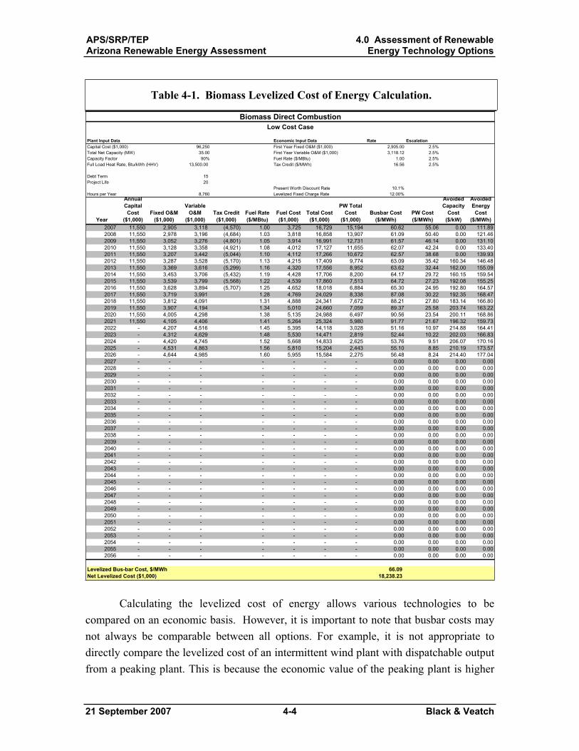
APS/SRP/TEPArizona Renewable Energy Assessment
4.0 Assessment of RenewableEnergy Technology Options
21 September 2007 4-4 Black & Veatch
Table 4-1. Biomass Levelized Cost of Energy Calculation.
Plant Input Data Economic Input Data Rate EscalationCapital Cost ($1,000) 96,250 First Year Fixed O&M ($1,000) 2,905.00 2.5%Total Net Capacity (MW) 35.00 First Year Variable O&M ($1,000) 3,118.12 2.5%Capacity Factor 90% Fuel Rate ($/MBtu) 1.00 2.5%Full Load Heat Rate, Btu/kWh (HHV) 13,500.00 Tax Credit ($/MWh) 16.56 2.5%
Debt Term 15 Project Life 20
Present Worth Discount Rate 10.1%Hours per Year 8,760 Levelized Fixed Charge Rate 12.00%
Year
AnnualCapital Cost
($1,000)Fixed O&M
($1,000)
Variable O&M
($1,000)Tax Credit
($1,000)Fuel Rate ($/MBtu)
Fuel Cost ($1,000)
Total Cost ($1,000)
PW Total Cost
($1,000)Busbar Cost
($/MWh)PW Cost ($/MWh)
AvoidedCapacity
Cost ($/kW)
AvoidedEnergy
Cost($/MWh)
2007 11,550 2,905 3,118 (4,570) 1.00 3,725 16,729 15,194 60.62 55.06 0.00 111.892008 11,550 2,978 3,196 (4,684) 1.03 3,818 16,858 13,907 61.09 50.40 0.00 121.462009 11,550 3,052 3,276 (4,801) 1.05 3,914 16,991 12,731 61.57 46.14 0.00 131.102010 11,550 3,128 3,358 (4,921) 1.08 4,012 17,127 11,655 62.07 42.24 0.00 133.402011 11,550 3,207 3,442 (5,044) 1.10 4,112 17,266 10,672 62.57 38.68 0.00 139.932012 11,550 3,287 3,528 (5,170) 1.13 4,215 17,409 9,774 63.09 35.42 160.34 146.482013 11,550 3,369 3,616 (5,299) 1.16 4,320 17,556 8,952 63.62 32.44 162.00 155.092014 11,550 3,453 3,706 (5,432) 1.19 4,428 17,706 8,200 64.17 29.72 160.15 159.542015 11,550 3,539 3,799 (5,568) 1.22 4,539 17,860 7,513 64.72 27.23 192.08 155.252016 11,550 3,628 3,894 (5,707) 1.25 4,652 18,018 6,884 65.30 24.95 192.80 164.572017 11,550 3,719 3,991 1.28 4,769 24,029 8,338 87.08 30.22 192.35 168.472018 11,550 3,812 4,091 1.31 4,888 24,341 7,672 88.21 27.80 183.14 166.802019 11,550 3,907 4,194 1.34 5,010 24,660 7,059 89.37 25.58 203.74 163.222020 11,550 4,005 4,298 1.38 5,135 24,988 6,497 90.56 23.54 200.11 168.862021 11,550 4,105 4,406 1.41 5,264 25,324 5,980 91.77 21.67 196.32 159.732022 - 4,207 4,516 1.45 5,395 14,118 3,028 51.16 10.97 214.88 164.412023 - 4,312 4,629 1.48 5,530 14,471 2,819 52.44 10.22 202.03 166.832024 - 4,420 4,745 1.52 5,668 14,833 2,625 53.76 9.51 206.07 170.162025 - 4,531 4,863 1.56 5,810 15,204 2,443 55.10 8.85 210.19 173.572026 - 4,644 4,985 1.60 5,955 15,584 2,275 56.48 8.24 214.40 177.042027 - - - - - - - 0.00 0.00 0.00 0.002028 - - - - - - - 0.00 0.00 0.00 0.002029 - - - - - - - 0.00 0.00 0.00 0.002030 - - - - - - - 0.00 0.00 0.00 0.002031 - - - - - - - 0.00 0.00 0.00 0.002032 - - - - - - - 0.00 0.00 0.00 0.002033 - - - - - - - 0.00 0.00 0.00 0.002034 - - - - - - - 0.00 0.00 0.00 0.002035 - - - - - - - 0.00 0.00 0.00 0.002036 - - - - - - - 0.00 0.00 0.00 0.002037 - - - - - - - 0.00 0.00 0.00 0.002038 - - - - - - - 0.00 0.00 0.00 0.002039 - - - - - - - 0.00 0.00 0.00 0.002040 - - - - - - - 0.00 0.00 0.00 0.002041 - - - - - - - 0.00 0.00 0.00 0.002042 - - - - - - - 0.00 0.00 0.00 0.002043 - - - - - - - 0.00 0.00 0.00 0.002044 - - - - - - - 0.00 0.00 0.00 0.002045 - - - - - - - 0.00 0.00 0.00 0.002046 - - - - - - - 0.00 0.00 0.00 0.002047 - - - - - - - 0.00 0.00 0.00 0.002048 - - - - - - - 0.00 0.00 0.00 0.002049 - - - - - - - 0.00 0.00 0.00 0.002050 - - - - - - - 0.00 0.00 0.00 0.002051 - - - - - - - 0.00 0.00 0.00 0.002052 - - - - - - - 0.00 0.00 0.00 0.002053 - - - - - - - 0.00 0.00 0.00 0.002054 - - - - - - - 0.00 0.00 0.00 0.002055 - - - - - - - 0.00 0.00 0.00 0.002056 - - - - - - - 0.00 0.00 0.00 0.00
66.09 18,238.23
Low Cost Case
Levelized Bus-bar Cost, $/MWhNet Levelized Cost ($1,000)
Biomass Direct Combustion
Calculating the levelized cost of energy allows various technologies to be compared on an economic basis. However, it is important to note that busbar costs may not always be comparable between all options. For example, it is not appropriate to directly compare the levelized cost of an intermittent wind plant with dispatchable output from a peaking plant. This is because the economic value of the peaking plant is higher
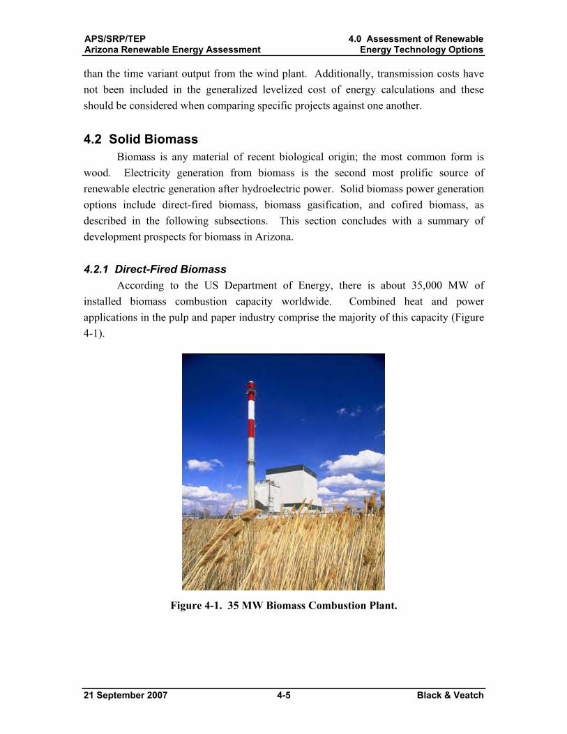
APS/SRP/TEPArizona Renewable Energy Assessment
4.0 Assessment of RenewableEnergy Technology Options
21 September 2007 4-5 Black & Veatch
than the time variant output from the wind plant. Additionally, transmission costs have not been included in the generalized levelized cost of energy calculations and these should be considered when comparing specific projects against one another.
4.2 Solid Biomass Biomass is any material of recent biological origin; the most common form is
wood. Electricity generation from biomass is the second most prolific source of renewable electric generation after hydroelectric power. Solid biomass power generation options include direct-fired biomass, biomass gasification, and cofired biomass, as described in the following subsections. This section concludes with a summary of development prospects for biomass in Arizona.
4.2.1 Direct-Fired Biomass According to the US Department of Energy, there is about 35,000 MW of
installed biomass combustion capacity worldwide. Combined heat and power applications in the pulp and paper industry comprise the majority of this capacity (Figure 4-1).
Figure 4-1. 35 MW Biomass Combustion Plant.
APS/SRP/TEPArizona Renewable Energy Assessment
4.0 Assessment of RenewableEnergy Technology Options
21 September 2007 4-6 Black & Veatch
Operating Principles Direct biomass combustion power plants in operation today use the same steam
Rankine cycle that was introduced commercially 100 years ago. In many respects, biomass power plants are similar to coal plants. When burning biomass, pressurized steam is produced in a boiler and then expanded through a turbine to produce electricity. Prior to its combustion in the boiler, the biomass fuel may require processing to improve the physical and chemical properties of the feedstock. Furnaces used in biomass combustion include spreader stoker fired, suspension fired, fluidized bed, cyclone, and pile burners. Advanced technologies, such as integrated biomass gasification combined cycle (IGCC), Plasma Gasification and biomass pyrolysis, are currently under development.
Applications Although wood is the most common biomass fuel, other biomass fuels include
agricultural residues such as bagasse (sugar cane residues), dried manure and sewage sludge, black liquor from pulp mills, and dedicated fuel crops such as fast growing grasses and eucalyptus.
Biomass plants usually have a capacity of less than 50 MW because of the dispersed nature of the feedstock and the large quantities of fuel required. As a result of the smaller scale of the plants and lower heating values of the fuels, biomass plants are commonly less efficient than modern fossil fuel plants. In addition to being less efficient, biomass is generally more expensive than conventional fossil fuels on a $/MBtu basis because of added transportation costs. These factors usually limit the use of direct-fired biomass technology to inexpensive or waste biomass sources.
Resource Availability To be economically feasible, dedicated biomass plants are located either at the
source of a fuel supply (such as at a sawmill) or within 50 miles of numerous suppliers (up to 200 miles for a very high quantity, low cost supplier). Wood and wood waste are the primary biomass resources and are typically concentrated in areas of high forest-product industry activity. In rural areas, agricultural production can often yield significant fuel resources that can be collected and burned in biomass plants. These agricultural resources include bagasse, corn stover, rice hulls, wheat straw, and other residues. Energy crops, such as switchgrass and short rotation woody crops, have also been identified as potential biomass sources. In urban areas, biomass is typically composed of wood wastes such as construction debris, pallets, yard and tree trimmings, and railroad ties. Locally grown and collected biomass fuels are relatively labor intensive
APS/SRP/TEPArizona Renewable Energy Assessment
4.0 Assessment of RenewableEnergy Technology Options
21 September 2007 4-7 Black & Veatch
and can provide substantial employment benefits to rural economies. In general, the availability of sufficient quantities of biomass is less of a feasibility concern than the high costs associated with transportation and delivery of the fuel.
Based on recent biomass resource assessments that Black & Veatch is familiar with, the expected cost of clean wood residues can vary as much as 100 percent depending on the type of residue, quantity, and hauling distance.
Cost and Performance Characteristics Table 4-2 presents the typical characteristics of a 35 MW stoker boiler biomass
plant with Rankine cycle using wood as fuel. Two fuel costs scenarios were evaluated: (1) a relatively lower cost ($1.00/MBtu) scenario which would be based primarily on urban wood waste sources in the major metropolitan areas, and (2) a moderate cost ($2.50/MBtu) scenario which would be more representative of a project using forest thinnings and forestry residues. Actual fuel cost could vary significantly from the values characterized here based on local supply and demand, and transportation distance. For example, Black & Veatch has previously estimated costs for biomass resources at greater than $3/MBtu in some parts of Arizona. In this case, transport distances were up to 200 miles. (Additional discussion is provided in Section 5.) Another possible biomass fuel is dedicated energy crops, which are grown specifically to provide feedstock for biomass plants. However, experience with energy crops is very limited in Arizona; further, costs for these fuels would likely approach $4.00/MBtu or greater. For these reasons, electricity costs for energy crops are not provided.
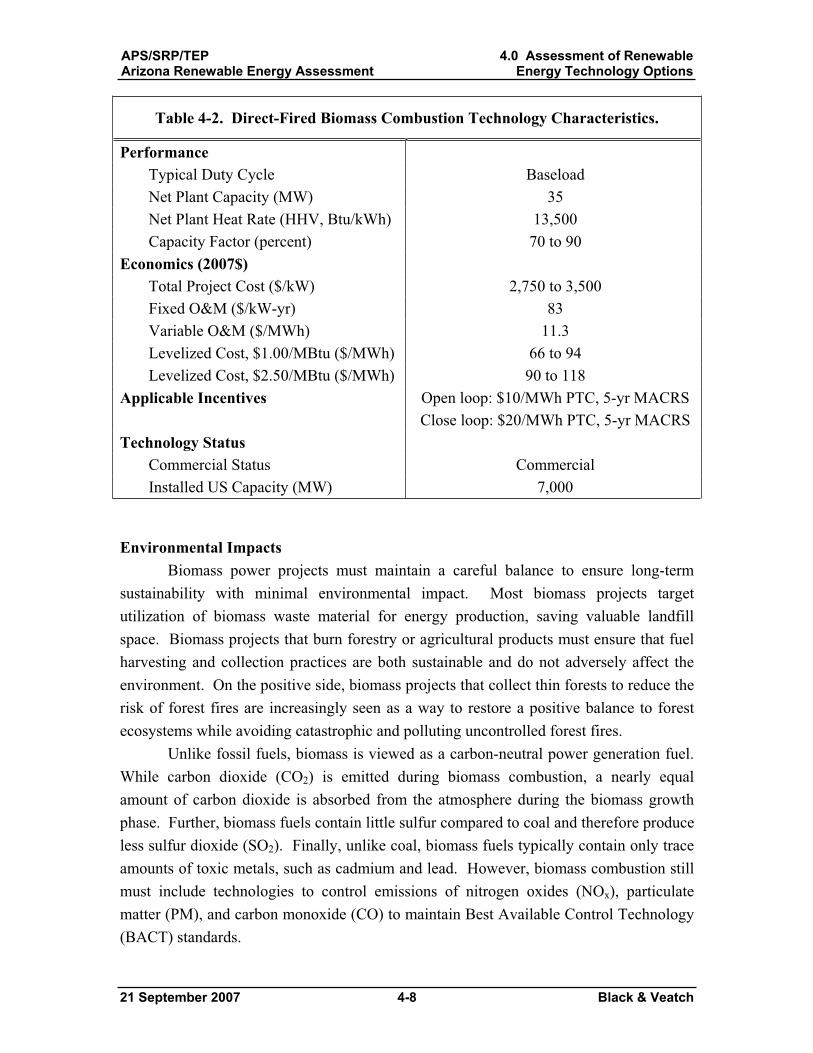
APS/SRP/TEPArizona Renewable Energy Assessment
4.0 Assessment of RenewableEnergy Technology Options
21 September 2007 4-8 Black & Veatch
Table 4-2. Direct-Fired Biomass Combustion Technology Characteristics.
PerformanceTypical Duty Cycle Baseload Net Plant Capacity (MW) 35 Net Plant Heat Rate (HHV, Btu/kWh) 13,500 Capacity Factor (percent) 70 to 90
Economics (2007$) Total Project Cost ($/kW) 2,750 to 3,500 Fixed O&M ($/kW-yr) 83 Variable O&M ($/MWh) 11.3 Levelized Cost, $1.00/MBtu ($/MWh) 66 to 94 Levelized Cost, $2.50/MBtu ($/MWh) 90 to 118
Applicable Incentives Open loop: $10/MWh PTC, 5-yr MACRS Close loop: $20/MWh PTC, 5-yr MACRS
Technology Status Commercial Status Commercial Installed US Capacity (MW) 7,000
Environmental Impacts Biomass power projects must maintain a careful balance to ensure long-term
sustainability with minimal environmental impact. Most biomass projects target utilization of biomass waste material for energy production, saving valuable landfill space. Biomass projects that burn forestry or agricultural products must ensure that fuel harvesting and collection practices are both sustainable and do not adversely affect the environment. On the positive side, biomass projects that collect thin forests to reduce the risk of forest fires are increasingly seen as a way to restore a positive balance to forest ecosystems while avoiding catastrophic and polluting uncontrolled forest fires.
Unlike fossil fuels, biomass is viewed as a carbon-neutral power generation fuel. While carbon dioxide (CO2) is emitted during biomass combustion, a nearly equal amount of carbon dioxide is absorbed from the atmosphere during the biomass growth phase. Further, biomass fuels contain little sulfur compared to coal and therefore produce less sulfur dioxide (SO2). Finally, unlike coal, biomass fuels typically contain only trace amounts of toxic metals, such as cadmium and lead. However, biomass combustion still must include technologies to control emissions of nitrogen oxides (NOx), particulate matter (PM), and carbon monoxide (CO) to maintain Best Available Control Technology (BACT) standards.
APS/SRP/TEPArizona Renewable Energy Assessment
4.0 Assessment of RenewableEnergy Technology Options
21 September 2007 4-9 Black & Veatch
Arizona Biomass Combustion Outlook The outlook for biomass combustion technologies is provided in Section 4.2.5
Biomass Technologies Development Prospects.
4.2.2 Biomass Gasification and IGCC Biomass gasification is an emerging technology that converts solid biomass into a
gaseous fuel which can then be combusted or otherwise utilized. There are numerous uses for the gas and many different gasifier technologies. Integrated gasification combined cycle (IGCC) is a developing application that combines a gasifier with a conventional combined cycle power plant (combustion turbine followed by a steam cycle). All of the 19 demonstration scale of IGCC plants constructed worldwide have been fossil-fueled. There are no integrated gasification combined cycle plants currently operating with biomass as a primary fuel.
Operating Principles Biomass gasification is a process to convert solid biomass into a gaseous fuel.
This is accomplished by heating the biomass in an environment low in oxygen (“fuel rich”). Gasification is a promising process for biomass conversion. By converting solid fuel to a combustible gas, gasification enables the use of more advanced, efficient and environmentally benign energy conversion processes such as gas turbines and fuel cells to produce power, and chemical synthesis to produce ethanol and other value added products. There is a huge variety of gasification technologies including updraft, downdraft, fixed grate, entrained flow, fluidized bed, and molten metal baths. The technology choice depends primarily on the fuel characteristics and the desired capacity of the plant.
Most biomass gasification systems are air blown. The primary product of air-blown gasification is a low heating value fuel gas, typically 15 to 20 percent (150-200 Btu/ft3) of the heating value of natural gas (1,000 Btu/ft3). Using oxygen, steam, or indirect heating results in a higher quality gas, although at higher costs.
Applications The primary advantage of gasification over direct combustion is the versatility of
the gasification product. Gasification expands the use of solid fuel to include practically all the uses of natural gas and petroleum, including close-coupled boilers, combustion engines and turbines, fuel cells, and chemical synthesis, and Stirling engines. The various fuel gas conversion options are illustrated in Figure 4-2.
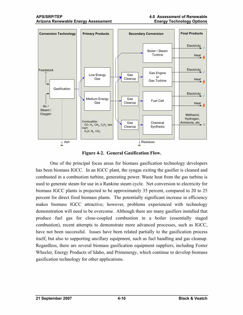
APS/SRP/TEPArizona Renewable Energy Assessment
4.0 Assessment of RenewableEnergy Technology Options
21 September 2007 4-10 Black & Veatch
Final Products
Gasification
Medium EnergyGas
Low EnergyGas
Combustible: CO, H2, CH4, CxHy, tarsInert: H2O, N2, CO2
Conversion Technology Primary Products
Fuel Cell
Gas Engineor
Gas Turbine
Boiler / SteamTurbine
GasCleanup
ChemicalSynthesis
GasCleanup
GasCleanup
GasCleanup
Secondary Conversion
ResiduesAsh
Feedstock
Air /Steam /Oxygen
Electricity
Heat
Methanol,Hydrogen,
Ammonia, etc
Electricity
Heat
Electricity
Heat
Figure 4-2. General Gasification Flow.
One of the principal focus areas for biomass gasification technology developers has been biomass IGCC. In an IGCC plant, the syngas exiting the gasifier is cleaned and combusted in a combustion turbine, generating power. Waste heat from the gas turbine is used to generate steam for use in a Rankine steam cycle. Net conversion to electricity for biomass IGCC plants is projected to be approximately 35 percent, compared to 20 to 25 percent for direct fired biomass plants. The potentially significant increase in efficiency makes biomass IGCC attractive; however, problems experienced with technology demonstration will need to be overcome. Although there are many gasifiers installed that produce fuel gas for close-coupled combustion in a boiler (essentially staged combustion), recent attempts to demonstrate more advanced processes, such as IGCC, have not been successful. Issues have been related partially to the gasification process itself, but also to supporting ancillary equipment, such as fuel handling and gas cleanup. Regardless, there are several biomass gasification equipment suppliers, including Foster Wheeler, Energy Products of Idaho, and Primenergy, which continue to develop biomass gasification technology for other applications.
APS/SRP/TEPArizona Renewable Energy Assessment
4.0 Assessment of RenewableEnergy Technology Options
21 September 2007 4-11 Black & Veatch
Resource Availability A biomass gasification or biomass IGCC plant would have similar resource
availability issues as a direct-fired biomass plant. To be economically feasible it should be located either at the source of a fuel supply or within 50 to 75 miles of numerous suppliers. Wood, wood byproducts, agricultural residues, energy crops, and urban wood wastes are all suitable fuels for a biomass IGCC plant.
Like other biomass conversion technologies, an IGCC biomass plant would be limited in capacity by the amount of resource which could feasibly be delivered. A reasonable estimate for this limit is 30 MW to 75 MW, depending on location. Conversely, coal IGCC power plants are typically limited by the gas turbine capacity, not by fuel availability, and can be designed for much larger capacities similar to other fossil fuel power plants.
Cost and Performance Characteristics Given the lack of commercial experience, cost and performance estimates for an
IGCC biomass plant are uncertain. Since it would be limited to a size much smaller than an IGCC coal plant, an IGCC biomass plant would not benefit from the economies of scale of such plants. Table 4-3 presents projected characteristics for a biomass IGCC combustion plant for urban wood waste and forest residues.
Environmental Impacts A biomass IGCC biomass project would have the same long-term sustainability
concerns as other biomass conversion technologies. Biomass is viewed as a carbon-neutral power generation fuel. While CO2 is emitted during biomass conversion, a nearly equal amount of CO2 is absorbed from the atmosphere during the biomass growth phase. Further, biomass fuels contain little sulfur compared to coal and therefore produce less SO2. Finally, unlike coal, biomass fuels typically contain only trace amounts of toxic metals, such as cadmium, and lead. Biomass gasification technologies will require equipment to control emissions of NOx, PM, and CO to maintain air emission standards. It is important to note that given that biomass IGCC is expected to have higher efficiency than biomass combustion-based power plants, the pounds of pollution per MWh generated are substantially less.
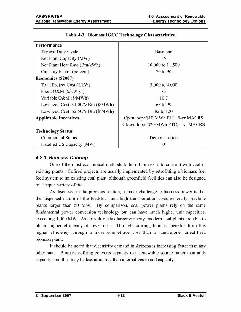
APS/SRP/TEPArizona Renewable Energy Assessment
4.0 Assessment of RenewableEnergy Technology Options
21 September 2007 4-12 Black & Veatch
Table 4-3. Biomass IGCC Technology Characteristics.
PerformanceTypical Duty Cycle Baseload Net Plant Capacity (MW) 35 Net Plant Heat Rate (Btu/kWh) 10,000 to 11,500 Capacity Factor (percent) 70 to 90
Economics ($2007) Total Project Cost ($/kW) 3,000 to 4,000 Fixed O&M ($/kW-yr) 83 Variable O&M ($/MWh) 10.7 Levelized Cost, $1.00/MBtu ($/MWh) 65 to 99 Levelized Cost, $2.50/MBtu ($/MWh) 82 to 120
Applicable Incentives Open loop: $10/MWh PTC, 5-yr MACRS Closed loop: $20/MWh PTC, 5-yr MACRS
Technology Status Commercial Status Demonstration Installed US Capacity (MW) 0
4.2.3 Biomass Cofiring One of the most economical methods to burn biomass is to cofire it with coal in
existing plants. Cofired projects are usually implemented by retrofitting a biomass fuel feed system to an existing coal plant, although greenfield facilities can also be designed to accept a variety of fuels.
As discussed in the previous section, a major challenge to biomass power is that the dispersed nature of the feedstock and high transportation costs generally preclude plants larger than 50 MW. By comparison, coal power plants rely on the same fundamental power conversion technology but can have much higher unit capacities, exceeding 1,000 MW. As a result of this larger capacity, modern coal plants are able to obtain higher efficiency at lower cost. Through cofiring, biomass benefits from this higher efficiency through a more competitive cost than a stand-alone, direct-fired biomass plant.
It should be noted that electricity demand in Arizona is increasing faster than any other state. Biomass cofiring converts capacity to a renewable source rather than adds capacity, and thus may be less attractive than alternatives to add capacity.
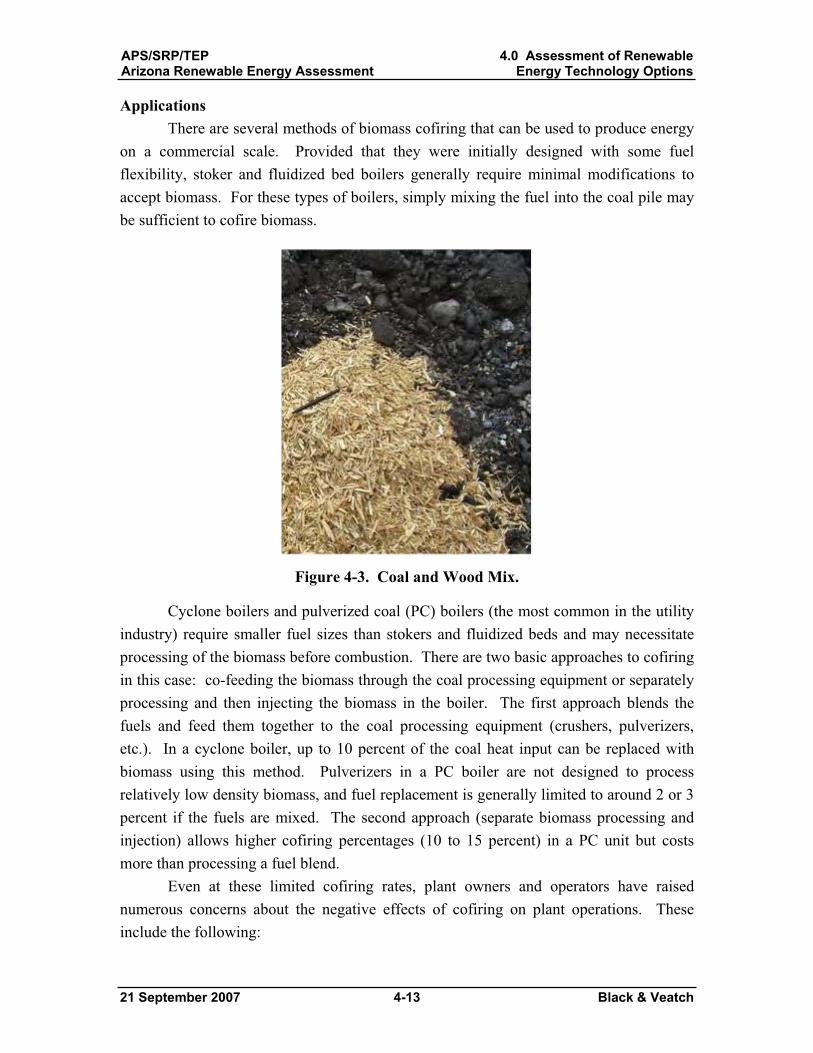
APS/SRP/TEPArizona Renewable Energy Assessment
4.0 Assessment of RenewableEnergy Technology Options
21 September 2007 4-13 Black & Veatch
Applications There are several methods of biomass cofiring that can be used to produce energy
on a commercial scale. Provided that they were initially designed with some fuel flexibility, stoker and fluidized bed boilers generally require minimal modifications to accept biomass. For these types of boilers, simply mixing the fuel into the coal pile may be sufficient to cofire biomass.
Figure 4-3. Coal and Wood Mix.
Cyclone boilers and pulverized coal (PC) boilers (the most common in the utility industry) require smaller fuel sizes than stokers and fluidized beds and may necessitate processing of the biomass before combustion. There are two basic approaches to cofiring in this case: co-feeding the biomass through the coal processing equipment or separately processing and then injecting the biomass in the boiler. The first approach blends the fuels and feed them together to the coal processing equipment (crushers, pulverizers, etc.). In a cyclone boiler, up to 10 percent of the coal heat input can be replaced with biomass using this method. Pulverizers in a PC boiler are not designed to process relatively low density biomass, and fuel replacement is generally limited to around 2 or 3 percent if the fuels are mixed. The second approach (separate biomass processing and injection) allows higher cofiring percentages (10 to 15 percent) in a PC unit but costs more than processing a fuel blend.
Even at these limited cofiring rates, plant owners and operators have raised numerous concerns about the negative effects of cofiring on plant operations. These include the following:
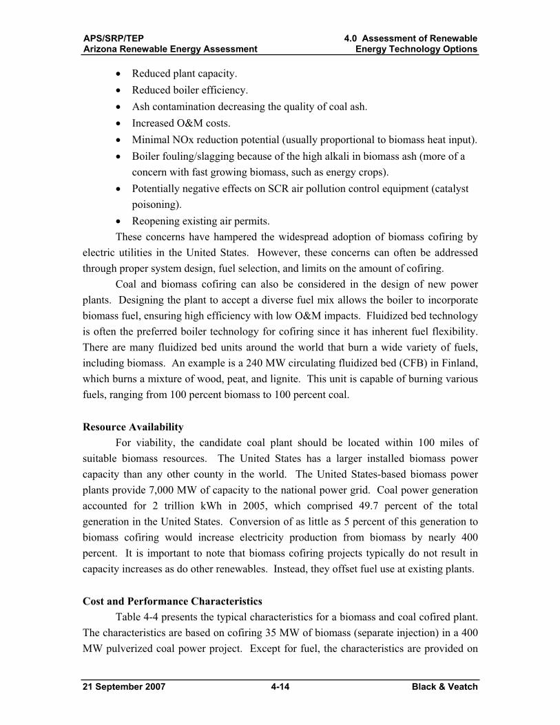
APS/SRP/TEPArizona Renewable Energy Assessment
4.0 Assessment of RenewableEnergy Technology Options
21 September 2007 4-14 Black & Veatch
Reduced plant capacity. Reduced boiler efficiency. Ash contamination decreasing the quality of coal ash. Increased O&M costs. Minimal NOx reduction potential (usually proportional to biomass heat input). Boiler fouling/slagging because of the high alkali in biomass ash (more of a concern with fast growing biomass, such as energy crops). Potentially negative effects on SCR air pollution control equipment (catalyst poisoning).Reopening existing air permits.
These concerns have hampered the widespread adoption of biomass cofiring by electric utilities in the United States. However, these concerns can often be addressed through proper system design, fuel selection, and limits on the amount of cofiring.
Coal and biomass cofiring can also be considered in the design of new power plants. Designing the plant to accept a diverse fuel mix allows the boiler to incorporate biomass fuel, ensuring high efficiency with low O&M impacts. Fluidized bed technology is often the preferred boiler technology for cofiring since it has inherent fuel flexibility. There are many fluidized bed units around the world that burn a wide variety of fuels, including biomass. An example is a 240 MW circulating fluidized bed (CFB) in Finland, which burns a mixture of wood, peat, and lignite. This unit is capable of burning various fuels, ranging from 100 percent biomass to 100 percent coal.
Resource Availability For viability, the candidate coal plant should be located within 100 miles of
suitable biomass resources. The United States has a larger installed biomass power capacity than any other county in the world. The United States-based biomass power plants provide 7,000 MW of capacity to the national power grid. Coal power generation accounted for 2 trillion kWh in 2005, which comprised 49.7 percent of the total generation in the United States. Conversion of as little as 5 percent of this generation to biomass cofiring would increase electricity production from biomass by nearly 400 percent. It is important to note that biomass cofiring projects typically do not result in capacity increases as do other renewables. Instead, they offset fuel use at existing plants.
Cost and Performance Characteristics Table 4-4 presents the typical characteristics for a biomass and coal cofired plant.
The characteristics are based on cofiring 35 MW of biomass (separate injection) in a 400 MW pulverized coal power project. Except for fuel, the characteristics are provided on
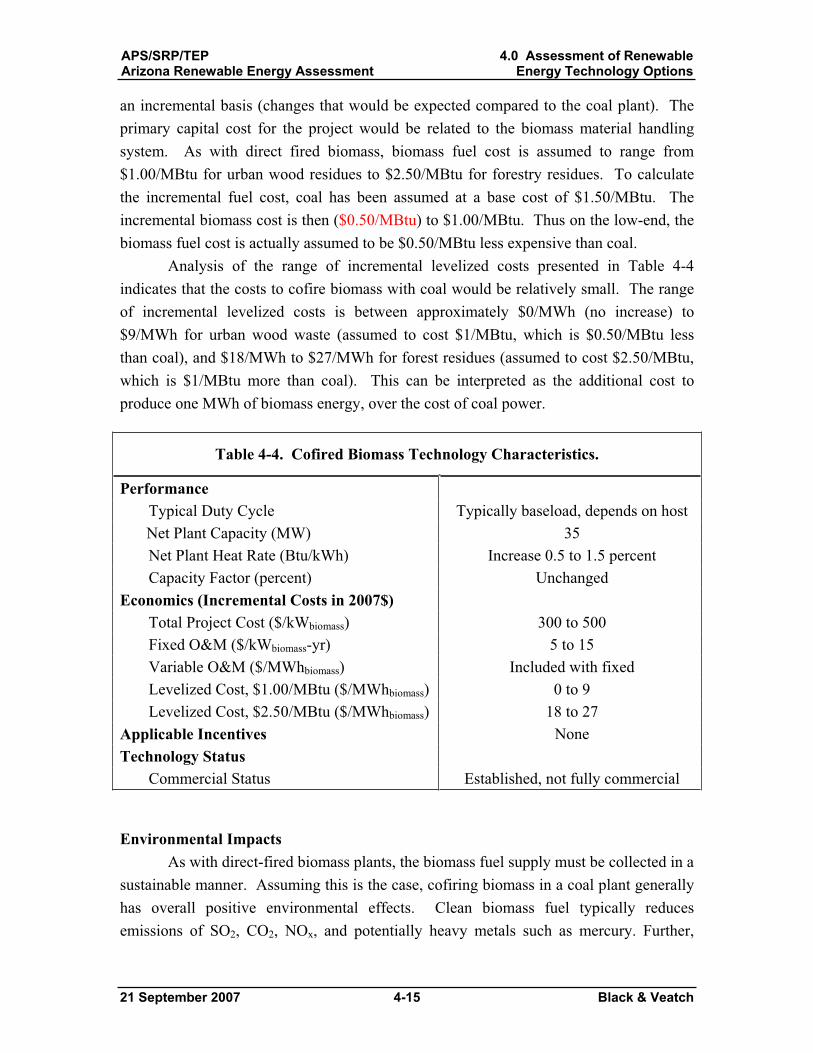
APS/SRP/TEPArizona Renewable Energy Assessment
4.0 Assessment of RenewableEnergy Technology Options
21 September 2007 4-15 Black & Veatch
an incremental basis (changes that would be expected compared to the coal plant). The primary capital cost for the project would be related to the biomass material handling system. As with direct fired biomass, biomass fuel cost is assumed to range from $1.00/MBtu for urban wood residues to $2.50/MBtu for forestry residues. To calculate the incremental fuel cost, coal has been assumed at a base cost of $1.50/MBtu. The incremental biomass cost is then ($0.50/MBtu) to $1.00/MBtu. Thus on the low-end, the biomass fuel cost is actually assumed to be $0.50/MBtu less expensive than coal.
Analysis of the range of incremental levelized costs presented in Table 4-4indicates that the costs to cofire biomass with coal would be relatively small. The range of incremental levelized costs is between approximately $0/MWh (no increase) to $9/MWh for urban wood waste (assumed to cost $1/MBtu, which is $0.50/MBtu less than coal), and $18/MWh to $27/MWh for forest residues (assumed to cost $2.50/MBtu, which is $1/MBtu more than coal). This can be interpreted as the additional cost to produce one MWh of biomass energy, over the cost of coal power.
Table 4-4. Cofired Biomass Technology Characteristics.
PerformanceTypical Duty Cycle Typically baseload, depends on host Net Plant Capacity (MW) 35 Net Plant Heat Rate (Btu/kWh) Increase 0.5 to 1.5 percent Capacity Factor (percent) Unchanged
Economics (Incremental Costs in 2007$) Total Project Cost ($/kWbiomass) 300 to 500 Fixed O&M ($/kWbiomass-yr) 5 to 15 Variable O&M ($/MWhbiomass) Included with fixed Levelized Cost, $1.00/MBtu ($/MWhbiomass) 0 to 9 Levelized Cost, $2.50/MBtu ($/MWhbiomass) 18 to 27
Applicable Incentives NoneTechnology Status
Commercial Status Established, not fully commercial
Environmental Impacts As with direct-fired biomass plants, the biomass fuel supply must be collected in a
sustainable manner. Assuming this is the case, cofiring biomass in a coal plant generally has overall positive environmental effects. Clean biomass fuel typically reduces emissions of SO2, CO2, NOx, and potentially heavy metals such as mercury. Further,
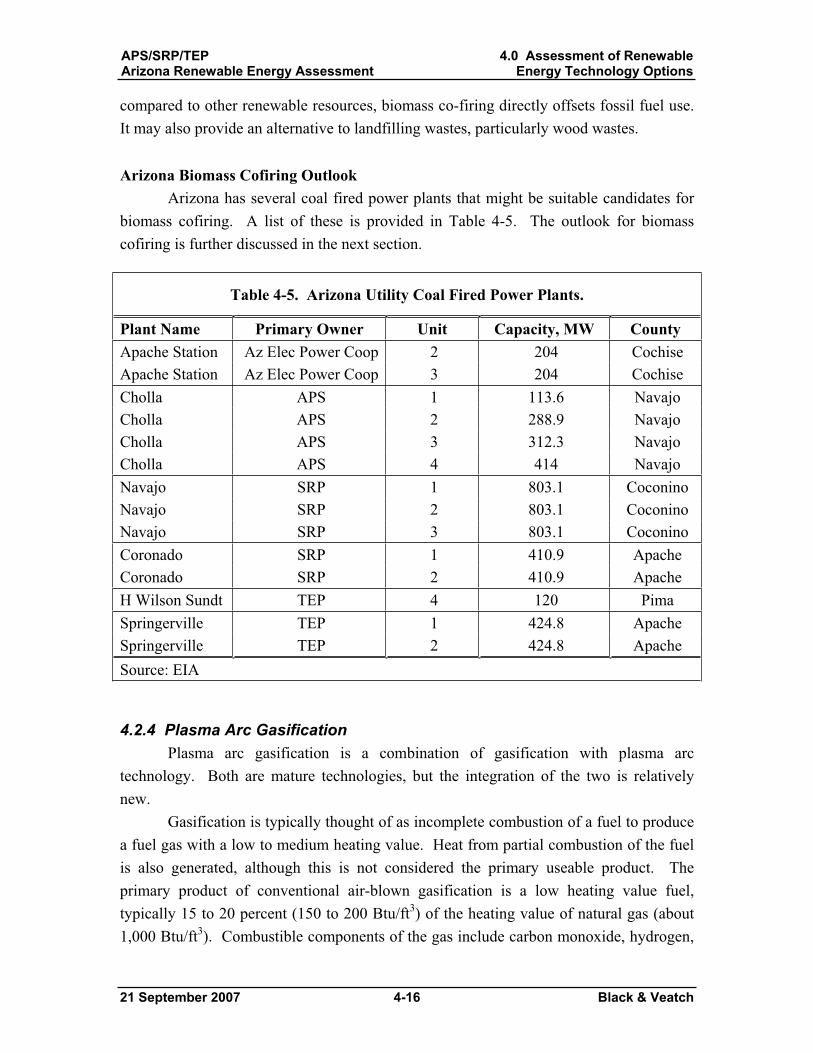
APS/SRP/TEPArizona Renewable Energy Assessment
4.0 Assessment of RenewableEnergy Technology Options
21 September 2007 4-16 Black & Veatch
compared to other renewable resources, biomass co-firing directly offsets fossil fuel use. It may also provide an alternative to landfilling wastes, particularly wood wastes.
Arizona Biomass Cofiring Outlook Arizona has several coal fired power plants that might be suitable candidates for
biomass cofiring. A list of these is provided in Table 4-5. The outlook for biomass cofiring is further discussed in the next section.
Table 4-5. Arizona Utility Coal Fired Power Plants.
Plant Name Primary Owner Unit Capacity, MW County Apache Station Az Elec Power Coop 2 204 Cochise Apache Station Az Elec Power Coop 3 204 Cochise Cholla APS 1 113.6 Navajo Cholla APS 2 288.9 Navajo Cholla APS 3 312.3 Navajo Cholla APS 4 414 Navajo Navajo SRP 1 803.1 Coconino Navajo SRP 2 803.1 Coconino Navajo SRP 3 803.1 Coconino Coronado SRP 1 410.9 Apache Coronado SRP 2 410.9 Apache H Wilson Sundt TEP 4 120 Pima Springerville TEP 1 424.8 Apache Springerville TEP 2 424.8 Apache Source: EIA
4.2.4 Plasma Arc Gasification Plasma arc gasification is a combination of gasification with plasma arc
technology. Both are mature technologies, but the integration of the two is relatively new.
Gasification is typically thought of as incomplete combustion of a fuel to produce a fuel gas with a low to medium heating value. Heat from partial combustion of the fuel is also generated, although this is not considered the primary useable product. The primary product of conventional air-blown gasification is a low heating value fuel, typically 15 to 20 percent (150 to 200 Btu/ft3) of the heating value of natural gas (about 1,000 Btu/ft3). Combustible components of the gas include carbon monoxide, hydrogen,

APS/SRP/TEPArizona Renewable Energy Assessment
4.0 Assessment of RenewableEnergy Technology Options
21 September 2007 4-17 Black & Veatch
methane, higher hydrocarbons such as ethane and propane, and tar. The conventional use for this gas is combustion in a boiler to generate steam, although it could potentially be used in higher efficiency engines or combustion turbines if the gas is sufficiently clean.
There are two primary configurations for plasma torches: transferred and non transferred torches. Both configurations use a pair of electrodes across which a large current is applied. An arc, basically manmade lightning, is created when the electricity bridges the gap between the two electrodes. The arc generates temperatures of up to 30,000 F. The transferred torch directly contacts the arc with the material, or a conductor, in the reactor. The non-transferred torch blows a stream of air across the arc inside the torch to produce superheated gas, approximately 5,000 F. This gas provides the thermal input to the reactor that is required to decompose the material. The temperature in the reactor itself is generally around 2,000 F. Plasma arc torches require large amounts of electricity. Depending on the fuel being processed, the facility may not generate net electricity output.
Figure 4-4. Plasma Arc Torch Operating (Source: http://www.zeusgroup.org/applications.html).
Applications The extreme temperatures produced by plasma torches makes them well-suited
for waste remediation applications because the inorganic constituents in the waste that might normally be hazardous are literally melted to form a glassy slag which can be
APS/SRP/TEPArizona Renewable Energy Assessment
4.0 Assessment of RenewableEnergy Technology Options
21 September 2007 4-18 Black & Veatch
captured in a solid form. This encapsulation of hazardous waste requires significant amounts of energy and has very specialized economical niche markets. Currently, some industry leaders feel that plasma arc disposal of municipal solid waste (MSW) is not economic. An alternate approach to strictly disposing of the MSW with plasma torches is to gasify the MSW and recover the combustible syngas that results from the thermal reaction. There are very few installations worldwide to benchmark against for economic evaluation. These are summarized in Table 4-6.
Table 4-6. Installed MSW Plasma Arc Gasification Projects.
Vendor - Project Fuel Commercial
Status
ElectricalCapacity,
MW
FuelThroughput,
tpdWestinghouse Plasma Corp.
Yoshii, Japan MSW Pilot -- 25 Utashinai, Japan ASR/MSW* Commercial 8 165 Mihama, Japan MSW Commercial -- 28
Startech EnvironmentalBristol, Connecticut Variety Demonstration -- 5
Integrated Environmental TechnologiesAPET, Hawaii Medical waste Commercial -- 24
Notes:* Primary fuel intended to be auto shredder residue (ASR). Plant is capable of using
MSW for up to 50 percent of volumetric throughput.
Resource Availability Plasma arc gasification technologies can process the same basic resources as other
biomass and waste to energy technologies. However, plasma arc is particularly well suited to handle difficult materials, such as hazardous waste, auto shredder residue, incinerator ash, low-level radioactive waste, and medical waste. The net power export potential (if any) of a plant depends heavily on the resource being processed.
Cost and Performance Characteristics Because the technology is pre-commercial, objective cost and performance
information for plasma arc systems was not obtainable for this study.
APS/SRP/TEPArizona Renewable Energy Assessment
4.0 Assessment of RenewableEnergy Technology Options
21 September 2007 4-19 Black & Veatch
Environmental Impacts Plasma arc technologies are well-suited for vitrification of waste materials.
Extensive documentation of testing shows that the vitreous slag has very low leaching potential, effectively “locking up” contaminants in the solid material. Air emissions are not as well-documented. Technology suppliers claim that the extreme temperatures of the plasma system dissociate any harmful molecular emissions. However, very little discussion of emissions such as mercury can be found. It does not seem that mercury would be captured in the slag because it has such a low boiling point. Conventional waste to energy facilities seem to have achieved compliance with EPA’s emissions limits for dioxins and furans; plasma arc gasification would not seem to offer substantial benefits over those technologies in that respect.
Arizona Plasma Gasification Development Prospects Plasma arc gasification of waste is a developmental technology that has not
gained widespread support, particularly as a power generation technology. There do seem to be some instances in which it can be cost effective, such as in highly land constrained areas with significant population density. Even in these favorable conditions, the economic viability of plasma arc projects is subject to technology risk. It is possible that plasma arc gasification of MSW may become commercial in a 10 to 20 year timeframe. In such case, it could be expected to generate approximately the same amount of electricity as other waste to energy options. Due to its pre-commercial nature, it is recommended that plasma arc gasification not be considered further for this study.
4.2.5 Biomass Technologies Development Prospects There is some potential to develop biomass resources, although they are relatively
limited compared to wind and solar resources in the state. Biomass potential is largely based on available resources; however, in the case of cofiring, a suitable host power plant in the vicinity is also necessary.
In December 2005, the National Renewable Energy Laboratory (NREL) published a new set of biomass resource data and documentation, including GIS data layers of major biomass resources on a county level. The data represents fairly uniform set of biomass resource data, and is the most current nation-wide, county level data source available. As described below, much of the resource data is based on statistical estimation. To determine the actual available quantities and suppliers of biomass material in the region, a more detailed resource assessment and supplier survey would be necessary. This survey would be carried out in the next phase of this project.
The NREL data is defined as follows:
APS/SRP/TEPArizona Renewable Energy Assessment
4.0 Assessment of RenewableEnergy Technology Options
21 September 2007 4-20 Black & Veatch
Agricultural Residues – This data includes residues from corn, wheat, soybeans, cotton, sorghum, barley, oats, rice, rye, canola, beans, peas, peanuts, potatoes, safflower, sunflower, sugarcane and flaxseed. Residue estimates were developed using the total grain production, crop-to-residue ratio, and moisture content. The total grain production data for each county in 2002 were as reported to the US Department of Agriculture. It was assumed that 35 percent of the total residue could be collected, accounting for residue left for soil protection, grazing, bedding, etc. Animal manures are discussed in the anaerobic digestion section of this report. Agricultural residues are relatively limited in Arizona due to the arid climate. Forest Residues – Forest residue data is adapted from the 2002 USDA Forest Service Timber Product Output Database. The quantities include commercial logging residues and other practices such as fire management (fuel reduction), pre-commercial thinnings, and land clearing. Since this data source is based on historical sector output, the NREL estimates have been augmented with an estimate of projected availability from fire management forest thinnings. A large portion of Arizona’s forested land is located within National Forests. Until the early 1990s, much of this land was harvested for timber. The amount of timber harvested has declined substantially over the past 15 years.Currently, much of the wood removed from Arizona forests is due to fire management. Primary Mill Residues – Primary mill residue data is also taken from the 2002 USDA Forest Service Timber Product Output Database. The quantities include mill residues such as slabs, edgings, trimmings, sawdust, veneer clippings, and pulp screenings. This includes material that is already utilized as well as material that is disposed as waste. As the amount of timber harvested from Arizona forests declined due to environmental restrictions, the timber available to sawmills also declined. This caused many of the sawmills in Arizona to close their operations. In 1960, there were approximately 38 sawmills; in 1998 there were only 13.5 In a recent Black & Veatch survey, even fewer mills were identified.
5 Source: Keegan, Charles E. Arizona’s Forest Products Industry: A Descriptive Analysis 1998. School of Business Administration, University of Montana
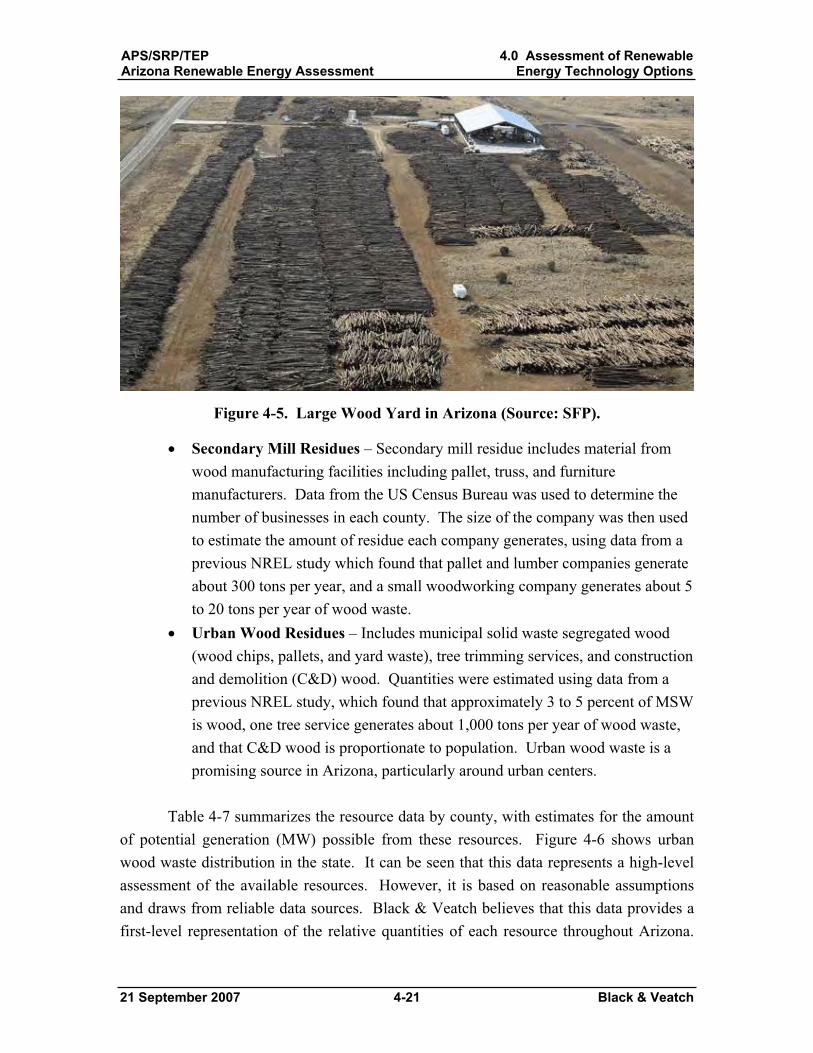
APS/SRP/TEPArizona Renewable Energy Assessment
4.0 Assessment of RenewableEnergy Technology Options
21 September 2007 4-21 Black & Veatch
Figure 4-5. Large Wood Yard in Arizona (Source: SFP).
Secondary Mill Residues – Secondary mill residue includes material from wood manufacturing facilities including pallet, truss, and furniture manufacturers. Data from the US Census Bureau was used to determine the number of businesses in each county. The size of the company was then used to estimate the amount of residue each company generates, using data from a previous NREL study which found that pallet and lumber companies generate about 300 tons per year, and a small woodworking company generates about 5 to 20 tons per year of wood waste. Urban Wood Residues – Includes municipal solid waste segregated wood (wood chips, pallets, and yard waste), tree trimming services, and construction and demolition (C&D) wood. Quantities were estimated using data from a previous NREL study, which found that approximately 3 to 5 percent of MSW is wood, one tree service generates about 1,000 tons per year of wood waste, and that C&D wood is proportionate to population. Urban wood waste is a promising source in Arizona, particularly around urban centers.
Table 4-7 summarizes the resource data by county, with estimates for the amount of potential generation (MW) possible from these resources. Figure 4-6 shows urban wood waste distribution in the state. It can be seen that this data represents a high-level assessment of the available resources. However, it is based on reasonable assumptions and draws from reliable data sources. Black & Veatch believes that this data provides a first-level representation of the relative quantities of each resource throughout Arizona.
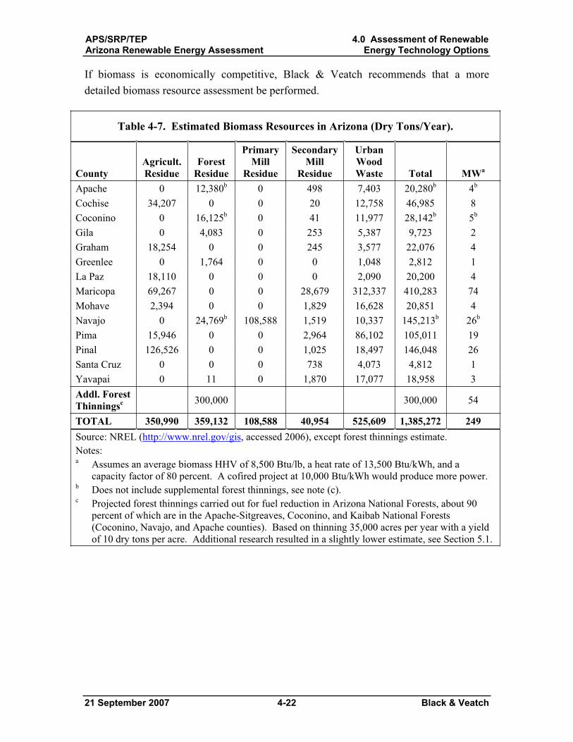
APS/SRP/TEPArizona Renewable Energy Assessment
4.0 Assessment of RenewableEnergy Technology Options
21 September 2007 4-22 Black & Veatch
If biomass is economically competitive, Black & Veatch recommends that a more detailed biomass resource assessment be performed.
Table 4-7. Estimated Biomass Resources in Arizona (Dry Tons/Year).
CountyAgricult.Residue
ForestResidue
Primary Mill
Residue
SecondaryMill
Residue
UrbanWoodWaste Total MWa
Apache 0 12,380b 0 498 7,403 20,280b 4b
Cochise 34,207 0 0 20 12,758 46,985 8 Coconino 0 16,125b 0 41 11,977 28,142b 5b
Gila 0 4,083 0 253 5,387 9,723 2 Graham 18,254 0 0 245 3,577 22,076 4 Greenlee 0 1,764 0 0 1,048 2,812 1 La Paz 18,110 0 0 0 2,090 20,200 4 Maricopa 69,267 0 0 28,679 312,337 410,283 74 Mohave 2,394 0 0 1,829 16,628 20,851 4 Navajo 0 24,769b 108,588 1,519 10,337 145,213b 26b
Pima 15,946 0 0 2,964 86,102 105,011 19 Pinal 126,526 0 0 1,025 18,497 146,048 26 Santa Cruz 0 0 0 738 4,073 4,812 1 Yavapai 0 11 0 1,870 17,077 18,958 3 Addl. Forest Thinningsc 300,000 300,000 54
TOTAL 350,990 359,132 108,588 40,954 525,609 1,385,272 249 Source: NREL (http://www.nrel.gov/gis, accessed 2006), except forest thinnings estimate. Notes:a Assumes an average biomass HHV of 8,500 Btu/lb, a heat rate of 13,500 Btu/kWh, and a
capacity factor of 80 percent. A cofired project at 10,000 Btu/kWh would produce more power. b Does not include supplemental forest thinnings, see note (c). c Projected forest thinnings carried out for fuel reduction in Arizona National Forests, about 90
percent of which are in the Apache-Sitgreaves, Coconino, and Kaibab National Forests (Coconino, Navajo, and Apache counties). Based on thinning 35,000 acres per year with a yield of 10 dry tons per acre. Additional research resulted in a slightly lower estimate, see Section 5.1.
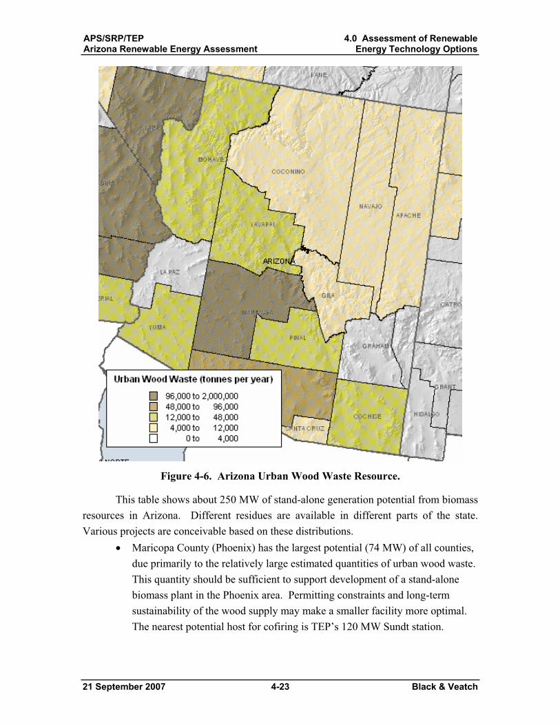
APS/SRP/TEPArizona Renewable Energy Assessment
4.0 Assessment of RenewableEnergy Technology Options
21 September 2007 4-23 Black & Veatch
Figure 4-6. Arizona Urban Wood Waste Resource.
This table shows about 250 MW of stand-alone generation potential from biomass resources in Arizona. Different residues are available in different parts of the state. Various projects are conceivable based on these distributions.
Maricopa County (Phoenix) has the largest potential (74 MW) of all counties, due primarily to the relatively large estimated quantities of urban wood waste. This quantity should be sufficient to support development of a stand-alone biomass plant in the Phoenix area. Permitting constraints and long-term sustainability of the wood supply may make a smaller facility more optimal. The nearest potential host for cofiring is TEP’s 120 MW Sundt station.
APS/SRP/TEPArizona Renewable Energy Assessment
4.0 Assessment of RenewableEnergy Technology Options
21 September 2007 4-24 Black & Veatch
In Pinal County, between Phoenix and Tucson, agricultural residues are predominant (26 MW total). Combined with the 19 MW residues from Pima County (Tucson), another biomass plant could be sited. Alternatively, the biomass could be cofired with coal in TEP’s Sundt station.As noted in the table, there may be 250,000 dry tons/year (45 MW) of forest thinnings from fuel reduction efforts in the Apache-Sitgreaves, Coconino, and Kaibab National Forests located in Coconino, Navajo, and Apache counties. In Navajo County alone there is a relatively large quantity of primary mill residues (20 MW worth). Much of this comes from a single source: the Fort Apache Timber Company’s (FATCO) sawmill located in the extreme southern portion of the county. The total resource potential from all sources in Coconino, Navajo, and Apache counties is 89 MW. The proposed 24 MW Snowflake White Mountain Power project will also burn some of the available biomass.
Additional assessment and quantification of potential biomass resources is provided in Section 5 of this report.
4.3 Biogas Biogas technology refers to the process of generating electricity with gas captured
from the anaerobic digestion of manure or naturally occurring landfill gas (LFG). The following subsections describe the formation of these fuels and their ability to produce renewable energy.
4.3.1 Anaerobic Digestion Anaerobic digestion is a natural process that occurs when bacteria decompose
organic materials in the absence of oxygen. The byproduct of this decomposition is generally composed of 50 to 80 percent methane. The most common applications of anaerobic digestion use industrial wastewater, animal manure, or human sewage as feedstock. According to Bioenergy News, the publication of the Bioenergy Association of New Zealand, Inc., the projection of total installed capacity of anaerobic digestion will grow from 185 MW in 2004 to 575 MW in 2013. The projection is that 203 MW will be installed in Western Europe, 68 MW in North America, and 46 MW in Australia.6
6The World Biomass Report, Bioenergy News, December 2004, http://www.bioenergy.org.nz.
APS/SRP/TEPArizona Renewable Energy Assessment
4.0 Assessment of RenewableEnergy Technology Options
21 September 2007 4-25 Black & Veatch
Applications Anaerobic digestion is commonly used in municipal wastewater treatment as a
first-stage treatment process for sewage sludge. Increasingly stringent agricultural manure and sewage treatment management regulations are the primary drivers for the heightened interest in anaerobic digestion technologies. Use of anaerobic digestion technologies in wastewater treatment applications results in a smaller quantity of biosolids residue compared to aerobic (digestion in the presence of oxygen) technologies Waste water treatment plants commonly use the biogas for process heating requirements. Power production from digestion facilities is typically a secondary consideration.
The Los Angeles Department of Water and Power has announced a new agreement to purchase power from a proposed 40 MW anaerobic digestion facility that will process 3,000 tons per day of municipal green waste, such as landscape trimmings and food waste to produce biogas for power production. The proposed facility would be the largest of its kind in the world. There are various other high-solids digestion systems installed worldwide, primarily in Europe and Japan.
Biogas produced by anaerobic digestion can be used for power generation, direct heat applications, and absorption chilling. Reciprocating engines are the most common power conversion device, although demonstrations with microturbines and fuel cells have been successful.
Resource Availability For manure digestion on farms, the resource is readily accessible, and only minor
modifications to existing manure management techniques are required to produce biogas suitable for power generation. In some cases, economies of scale may be realized by transporting manure from multiple farms to a central digestion facility. For central plant digestion of manure from several sources, the availability and proximity of a large number of livestock operations is necessary to provide sufficient manure feed rate to the facility. However, the larger size of regional facilities does not necessarily guarantee better economics, because of higher manure transportation costs. For anaerobic digestion of municipal sewage wastes, the resource is readily available at the wastewater treatment plant.
Cost and Performance Characteristics Table 4-8 presents the typical characteristics of farm-scale dairy manure
anaerobic digestion systems utilizing reciprocating engine technology. Costs for anaerobic digestion systems are very site specific. A photo of a dairy manure digester is shown on Figure 4-7.
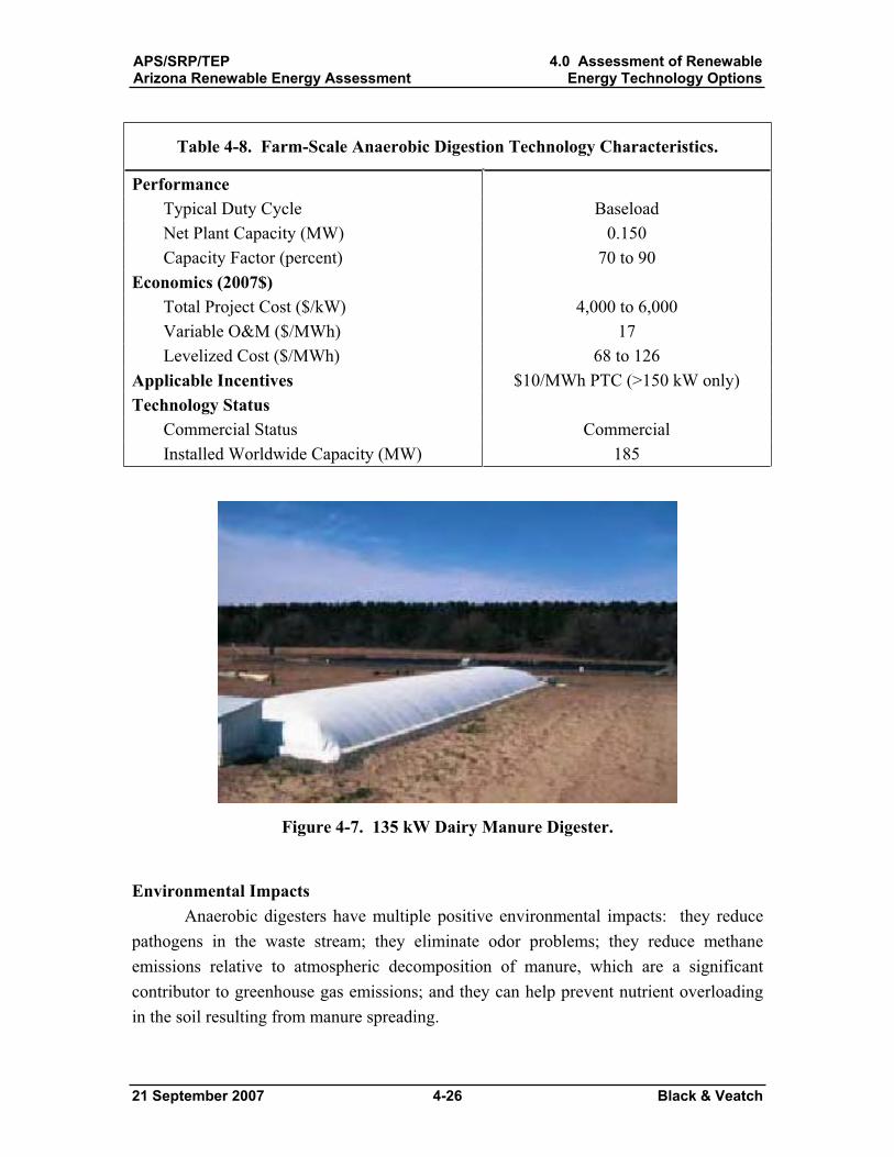
APS/SRP/TEPArizona Renewable Energy Assessment
4.0 Assessment of RenewableEnergy Technology Options
21 September 2007 4-26 Black & Veatch
Table 4-8. Farm-Scale Anaerobic Digestion Technology Characteristics.
PerformanceTypical Duty Cycle Baseload Net Plant Capacity (MW) 0.150 Capacity Factor (percent) 70 to 90
Economics (2007$) Total Project Cost ($/kW) 4,000 to 6,000 Variable O&M ($/MWh) 17 Levelized Cost ($/MWh) 68 to 126
Applicable Incentives $10/MWh PTC (>150 kW only) Technology Status
Commercial Status Commercial Installed Worldwide Capacity (MW) 185
Figure 4-7. 135 kW Dairy Manure Digester.
Environmental Impacts Anaerobic digesters have multiple positive environmental impacts: they reduce
pathogens in the waste stream; they eliminate odor problems; they reduce methane emissions relative to atmospheric decomposition of manure, which are a significant contributor to greenhouse gas emissions; and they can help prevent nutrient overloading in the soil resulting from manure spreading.
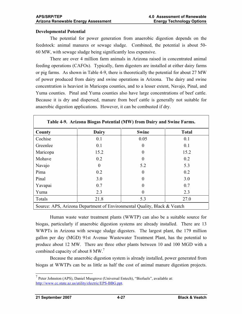
APS/SRP/TEPArizona Renewable Energy Assessment
4.0 Assessment of RenewableEnergy Technology Options
21 September 2007 4-27 Black & Veatch
Developmental Potential The potential for power generation from anaerobic digestion depends on the
feedstock: animal manures or sewage sludge. Combined, the potential is about 50-60 MW, with sewage sludge being significantly less expensive.
There are over 4 million farm animals in Arizona raised in concentrated animal feeding operations (CAFOs). Typically, farm digesters are installed at either dairy farms or pig farms. As shown in Table 4-9, there is theoretically the potential for about 27 MW of power produced from dairy and swine operations in Arizona. The dairy and swine concentration is heaviest in Maricopa counties, and to a lesser extent, Navajo, Pinal, and Yuma counties. Pinal and Yuma counties also have large concentrations of beef cattle. Because it is dry and dispersed, manure from beef cattle is generally not suitable for anaerobic digestion applications. However, it can be combusted if dry.
Table 4-9. Arizona Biogas Potential (MW) from Dairy and Swine Farms.
County Dairy Swine Total Cochise 0.1 0.05 0.1 Greenlee 0.1 0 0.1 Maricopa 15.2 0 15.2 Mohave 0.2 0 0.2 Navajo 0 5.2 5.3 Pima 0.2 0 0.2 Pinal 3.0 0 3.0 Yavapai 0.7 0 0.7 Yuma 2.3 0 2.3 Totals 21.8 5.3 27.0 Source: APS, Arizona Department of Environmental Quality, Black & Veatch
Human waste water treatment plants (WWTP) can also be a suitable source for biogas, particularly if anaerobic digestion systems are already installed. There are 13 WWPTs in Arizona with sewage sludge digesters. The largest plant, the 179 million gallon per day (MGD) 91st Avenue Wastewater Treatment Plant, has the potential to produce about 12 MW. There are three other plants between 10 and 100 MGD with a combined capacity of about 8 MW.7
Because the anaerobic digestion system is already installed, power generated from biogas at WWTPs can be as little as half the cost of animal manure digestion projects.
7 Peter Johnston (APS), Daniel Musgrove (Universal Entech), “Biofuels”, available at: http://www.cc.state.az.us/utility/electric/EPS-BBG.ppt.
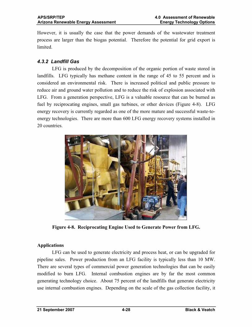
APS/SRP/TEPArizona Renewable Energy Assessment
4.0 Assessment of RenewableEnergy Technology Options
21 September 2007 4-28 Black & Veatch
However, it is usually the case that the power demands of the wastewater treatment process are larger than the biogas potential. Therefore the potential for grid export is limited.
4.3.2 Landfill Gas LFG is produced by the decomposition of the organic portion of waste stored in
landfills. LFG typically has methane content in the range of 45 to 55 percent and is considered an environmental risk. There is increased political and public pressure to reduce air and ground water pollution and to reduce the risk of explosion associated with LFG. From a generation perspective, LFG is a valuable resource that can be burned as fuel by reciprocating engines, small gas turbines, or other devices (Figure 4-8). LFG energy recovery is currently regarded as one of the more mature and successful waste-to-energy technologies. There are more than 600 LFG energy recovery systems installed in 20 countries.
Figure 4-8. Reciprocating Engine Used to Generate Power from LFG.
Applications LFG can be used to generate electricity and process heat, or can be upgraded for
pipeline sales. Power production from an LFG facility is typically less than 10 MW. There are several types of commercial power generation technologies that can be easily modified to burn LFG. Internal combustion engines are by far the most common generating technology choice. About 75 percent of the landfills that generate electricity use internal combustion engines. Depending on the scale of the gas collection facility, it
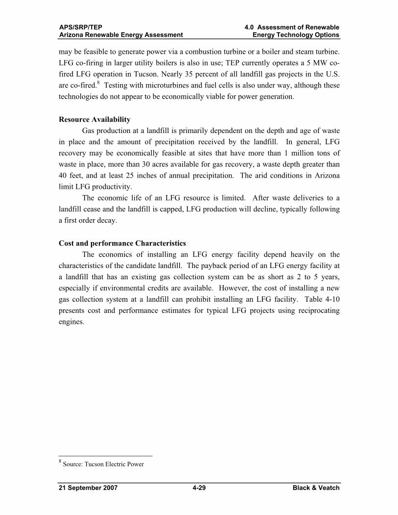
APS/SRP/TEPArizona Renewable Energy Assessment
4.0 Assessment of RenewableEnergy Technology Options
21 September 2007 4-29 Black & Veatch
may be feasible to generate power via a combustion turbine or a boiler and steam turbine. LFG co-firing in larger utility boilers is also in use; TEP currently operates a 5 MW co-fired LFG operation in Tucson. Nearly 35 percent of all landfill gas projects in the U.S. are co-fired.8 Testing with microturbines and fuel cells is also under way, although these technologies do not appear to be economically viable for power generation.
Resource Availability Gas production at a landfill is primarily dependent on the depth and age of waste
in place and the amount of precipitation received by the landfill. In general, LFG recovery may be economically feasible at sites that have more than 1 million tons of waste in place, more than 30 acres available for gas recovery, a waste depth greater than 40 feet, and at least 25 inches of annual precipitation. The arid conditions in Arizona limit LFG productivity.
The economic life of an LFG resource is limited. After waste deliveries to a landfill cease and the landfill is capped, LFG production will decline, typically following a first order decay.
Cost and performance Characteristics The economics of installing an LFG energy facility depend heavily on the
characteristics of the candidate landfill. The payback period of an LFG energy facility at a landfill that has an existing gas collection system can be as short as 2 to 5 years, especially if environmental credits are available. However, the cost of installing a new gas collection system at a landfill can prohibit installing an LFG facility. Table 4-10presents cost and performance estimates for typical LFG projects using reciprocating engines.
8 Source: Tucson Electric Power
APS/SRP/TEPArizona Renewable Energy Assessment
4.0 Assessment of RenewableEnergy Technology Options
21 September 2007 4-30 Black & Veatch
Table 4-10. Landfill Gas Technology Characteristics
PerformanceTypical Duty Cycle Baseload Net Plant Capacity (MW) 2 to 10 Capacity Factor (percent) 70 to 90
Economics (2007$) Total Project Cost ($/kW) 1,500 to 2,000 Variable O&M ($/MWh) 17 Fuel Cost ($/MBtu) 1.00 to 3.00*
Levelized Cost ($/MWh) 40 to 80 Applicable Incentives $10/MWh PTC Technology Status
Commercial Status Commercial Installed US Capacity (MW) 1,100
* Fuel cost is variable. The low end of this range is unlikely unless an existing gas purchase contract is in place, or responsibility for the gas collection system is assumed. .
Environmental Impacts Combustion of LFG releases pollutants similar to those released by many other
fuels, but the combustion of LFG is generally perceived as environmentally beneficial. Since LFG is principally composed of methane, if it is not combusted, LFG is released into the atmosphere as a greenhouse gas. As a greenhouse gas, methane is 23 times more harmful than CO2. Collecting the gas and converting the methane to CO2 through combustion greatly reduces the potency of LFG as a source of greenhouse gas emissions.
Arizona Landfill Gas Outlook The potential for landfill gas project developments in Arizona is limited, although
project economics are generally very competitive. Based on data acquired from the US Environmental Protection Agency’s (EPA) Landfill Methane Outreach Program (LMOP) database, there are at least 25 candidate landfills with the potential for power generation from landfill gas. These projects are listed in Table 4-11. The estimated potential generation at the different locations ranges from a few kilowatts up to around 10 MW. In aggregate, 20 to 30 MW of potential may be possible. The actual amount of generation which is achievable at these locations will depend on the actual gas generation levels, landfill gas composition, the level of coverage of the collection system, and the net plant heat rate (NPHR) of the engine-generators or other appropriate conversion technology.
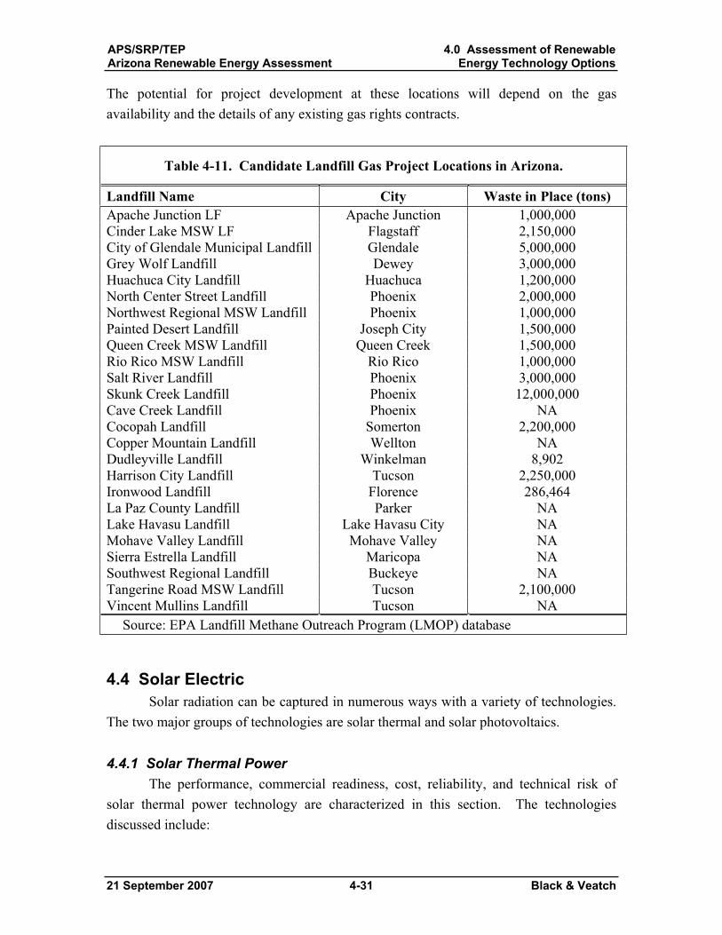
APS/SRP/TEPArizona Renewable Energy Assessment
4.0 Assessment of RenewableEnergy Technology Options
21 September 2007 4-31 Black & Veatch
The potential for project development at these locations will depend on the gas availability and the details of any existing gas rights contracts.
Table 4-11. Candidate Landfill Gas Project Locations in Arizona.
Landfill Name City Waste in Place (tons) Apache Junction LF Apache Junction 1,000,000 Cinder Lake MSW LF Flagstaff 2,150,000 City of Glendale Municipal Landfill Glendale 5,000,000 Grey Wolf Landfill Dewey 3,000,000 Huachuca City Landfill Huachuca 1,200,000 North Center Street Landfill Phoenix 2,000,000 Northwest Regional MSW Landfill Phoenix 1,000,000 Painted Desert Landfill Joseph City 1,500,000 Queen Creek MSW Landfill Queen Creek 1,500,000 Rio Rico MSW Landfill Rio Rico 1,000,000 Salt River Landfill Phoenix 3,000,000 Skunk Creek Landfill Phoenix 12,000,000 Cave Creek Landfill Phoenix NA Cocopah Landfill Somerton 2,200,000 Copper Mountain Landfill Wellton NA Dudleyville Landfill Winkelman 8,902 Harrison City Landfill Tucson 2,250,000 Ironwood Landfill Florence 286,464 La Paz County Landfill Parker NA Lake Havasu Landfill Lake Havasu City NA Mohave Valley Landfill Mohave Valley NA Sierra Estrella Landfill Maricopa NA Southwest Regional Landfill Buckeye NA Tangerine Road MSW Landfill Tucson 2,100,000 Vincent Mullins Landfill Tucson NA
Source: EPA Landfill Methane Outreach Program (LMOP) database
4.4 Solar Electric Solar radiation can be captured in numerous ways with a variety of technologies.
The two major groups of technologies are solar thermal and solar photovoltaics.
4.4.1 Solar Thermal Power The performance, commercial readiness, cost, reliability, and technical risk of
solar thermal power technology are characterized in this section. The technologies discussed include:
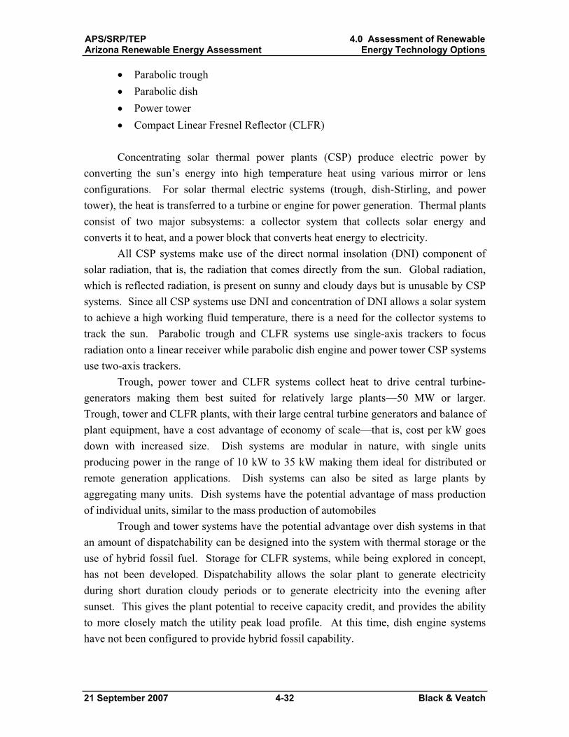
APS/SRP/TEPArizona Renewable Energy Assessment
4.0 Assessment of RenewableEnergy Technology Options
21 September 2007 4-32 Black & Veatch
Parabolic trough Parabolic dish Power tower Compact Linear Fresnel Reflector (CLFR)
Concentrating solar thermal power plants (CSP) produce electric power by converting the sun’s energy into high temperature heat using various mirror or lens configurations. For solar thermal electric systems (trough, dish-Stirling, and power tower), the heat is transferred to a turbine or engine for power generation. Thermal plants consist of two major subsystems: a collector system that collects solar energy and converts it to heat, and a power block that converts heat energy to electricity.
All CSP systems make use of the direct normal insolation (DNI) component of solar radiation, that is, the radiation that comes directly from the sun. Global radiation, which is reflected radiation, is present on sunny and cloudy days but is unusable by CSP systems. Since all CSP systems use DNI and concentration of DNI allows a solar system to achieve a high working fluid temperature, there is a need for the collector systems to track the sun. Parabolic trough and CLFR systems use single-axis trackers to focus radiation onto a linear receiver while parabolic dish engine and power tower CSP systems use two-axis trackers.
Trough, power tower and CLFR systems collect heat to drive central turbine-generators making them best suited for relatively large plants—50 MW or larger. Trough, tower and CLFR plants, with their large central turbine generators and balance of plant equipment, have a cost advantage of economy of scale—that is, cost per kW goes down with increased size. Dish systems are modular in nature, with single units producing power in the range of 10 kW to 35 kW making them ideal for distributed or remote generation applications. Dish systems can also be sited as large plants by aggregating many units. Dish systems have the potential advantage of mass production of individual units, similar to the mass production of automobiles
Trough and tower systems have the potential advantage over dish systems in that an amount of dispatchability can be designed into the system with thermal storage or the use of hybrid fossil fuel. Storage for CLFR systems, while being explored in concept, has not been developed. Dispatchability allows the solar plant to generate electricity during short duration cloudy periods or to generate electricity into the evening after sunset. This gives the plant potential to receive capacity credit, and provides the ability to more closely match the utility peak load profile. At this time, dish engine systems have not been configured to provide hybrid fossil capability.
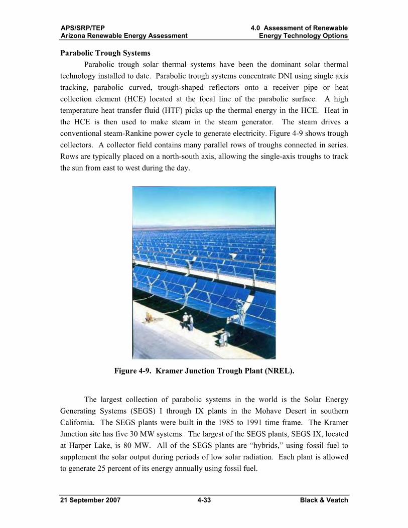
APS/SRP/TEPArizona Renewable Energy Assessment
4.0 Assessment of RenewableEnergy Technology Options
21 September 2007 4-33 Black & Veatch
Parabolic Trough Systems Parabolic trough solar thermal systems have been the dominant solar thermal
technology installed to date. Parabolic trough systems concentrate DNI using single axis tracking, parabolic curved, trough-shaped reflectors onto a receiver pipe or heat collection element (HCE) located at the focal line of the parabolic surface. A high temperature heat transfer fluid (HTF) picks up the thermal energy in the HCE. Heat in the HCE is then used to make steam in the steam generator. The steam drives a conventional steam-Rankine power cycle to generate electricity. Figure 4-9 shows trough collectors. A collector field contains many parallel rows of troughs connected in series. Rows are typically placed on a north-south axis, allowing the single-axis troughs to track the sun from east to west during the day.
Figure 4-9. Kramer Junction Trough Plant (NREL).
The largest collection of parabolic systems in the world is the Solar Energy Generating Systems (SEGS) I through IX plants in the Mohave Desert in southern California. The SEGS plants were built in the 1985 to 1991 time frame. The Kramer Junction site has five 30 MW systems. The largest of the SEGS plants, SEGS IX, located at Harper Lake, is 80 MW. All of the SEGS plants are “hybrids,” using fossil fuel to supplement the solar output during periods of low solar radiation. Each plant is allowed to generate 25 percent of its energy annually using fossil fuel.
APS/SRP/TEPArizona Renewable Energy Assessment
4.0 Assessment of RenewableEnergy Technology Options
21 September 2007 4-34 Black & Veatch
There are several commercial parabolic trough projects in the planning or active project development stage. Solargenix, (now Acciona) constructed a 1 MW plant in Arizona, which became operational in spring 2006. There are several plants under construction, including Nevada Solar One, an Acciona 64 MW plant in Nevada, and several 50 MW plants in Spain. The Andasol Spanish plants will include 7 hours of thermal storage. Other projects in various stages of planning include integrated solar combined cycle system (ISCCS) in southern California, India, Egypt, Morocco, Mexico, and Algeria. In addition, there are plans for a series of SEGS type plants in Israel.
Parabolic trough systems are considered commercially available for industrial applications. The primary developers of this technology include Acciona, Solel Solar Systems, Solar Millennium and Solucar. Suppliers of components for trough systems include reflector supplier Flabeg and receiver suppliers Schott Glass and Solel Solar Systems. Other major glass companies have expressed interest in entering the trough mirror market. The currently planned technology, for thermal storage, is the molten salt two-tank system. This provides a feasible storage capacity of up to 12 hours and is considered to have a low-to-moderate associated technology risk.
Parabolic Dish-Engine Systems A solar parabolic dish-engine system comprises of a solar concentrator (or
“parabolic dish”) and the power conversion unit (PCU). The concentrator consists of mirror facets which combine to form a parabolic dish. The dish redirects DNI to a receiver mounted on a boom at the dish’s focal point. The system uses a two-axis tracker such that it points at the sun continuously.
A parabolic dish-engine system using a Stirling engine is shown on Figure 4-10.The PCU includes the thermal receiver and the engine-generator. In the solar receiver, radiant solar energy is converted to heat in a closed hydrogen loop which drives the Stirling engine-generator. Because the PCUs are air cooled, water cooling is not required. This is important because water cooling is necessary for the large, central power blocks associated with trough and power tower technologies. Thermal storage is not currently considered to be a viable option for dish engine systems.
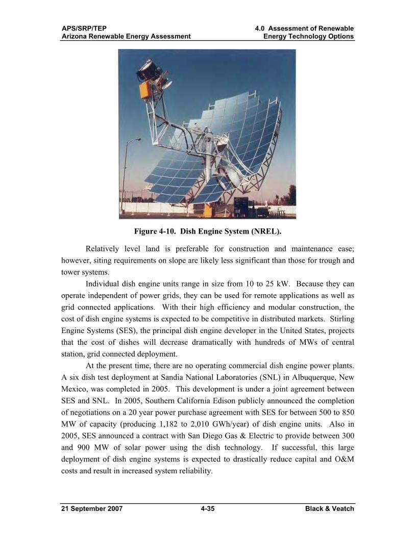
APS/SRP/TEPArizona Renewable Energy Assessment
4.0 Assessment of RenewableEnergy Technology Options
21 September 2007 4-35 Black & Veatch
Figure 4-10. Dish Engine System (NREL).
Relatively level land is preferable for construction and maintenance ease; however, siting requirements on slope are likely less significant than those for trough and tower systems.
Individual dish engine units range in size from 10 to 25 kW. Because they can operate independent of power grids, they can be used for remote applications as well as grid connected applications. With their high efficiency and modular construction, the cost of dish engine systems is expected to be competitive in distributed markets. Stirling Engine Systems (SES), the principal dish engine developer in the United States, projects that the cost of dishes will decrease dramatically with hundreds of MWs of central station, grid connected deployment.
At the present time, there are no operating commercial dish engine power plants. A six dish test deployment at Sandia National Laboratories (SNL) in Albuquerque, New Mexico, was completed in 2005. This development is under a joint agreement between SES and SNL. In 2005, Southern California Edison publicly announced the completion of negotiations on a 20 year power purchase agreement with SES for between 500 to 850 MW of capacity (producing 1,182 to 2,010 GWh/year) of dish engine units. Also in 2005, SES announced a contract with San Diego Gas & Electric to provide between 300 and 900 MW of solar power using the dish technology. If successful, this large deployment of dish engine systems is expected to drastically reduce capital and O&M costs and result in increased system reliability.
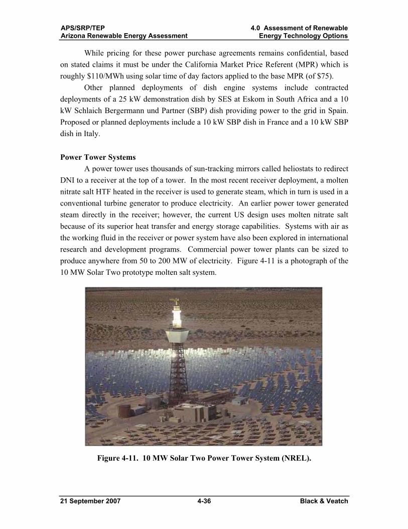
APS/SRP/TEPArizona Renewable Energy Assessment
4.0 Assessment of RenewableEnergy Technology Options
21 September 2007 4-36 Black & Veatch
While pricing for these power purchase agreements remains confidential, based on stated claims it must be under the California Market Price Referent (MPR) which is roughly $110/MWh using solar time of day factors applied to the base MPR (of $75).
Other planned deployments of dish engine systems include contracted deployments of a 25 kW demonstration dish by SES at Eskom in South Africa and a 10 kW Schlaich Bergermann und Partner (SBP) dish providing power to the grid in Spain. Proposed or planned deployments include a 10 kW SBP dish in France and a 10 kW SBP dish in Italy.
Power Tower Systems A power tower uses thousands of sun-tracking mirrors called heliostats to redirect
DNI to a receiver at the top of a tower. In the most recent receiver deployment, a molten nitrate salt HTF heated in the receiver is used to generate steam, which in turn is used in a conventional turbine generator to produce electricity. An earlier power tower generated steam directly in the receiver; however, the current US design uses molten nitrate salt because of its superior heat transfer and energy storage capabilities. Systems with air as the working fluid in the receiver or power system have also been explored in international research and development programs. Commercial power tower plants can be sized to produce anywhere from 50 to 200 MW of electricity. Figure 4-11 is a photograph of the 10 MW Solar Two prototype molten salt system.
Figure 4-11. 10 MW Solar Two Power Tower System (NREL).
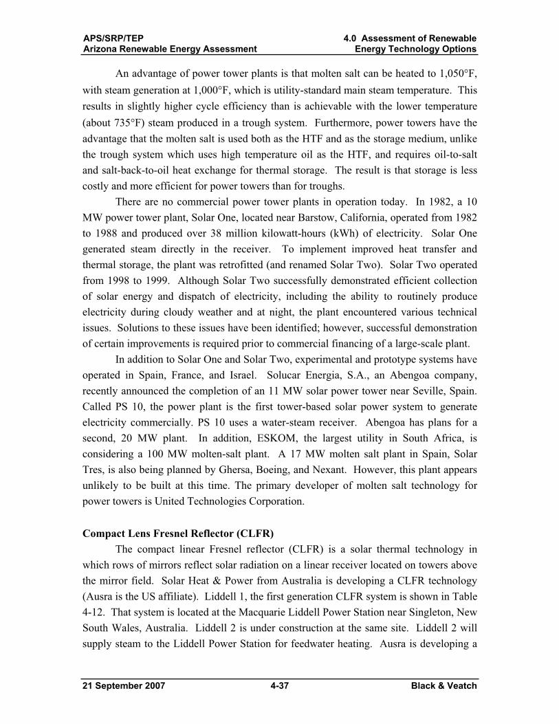
APS/SRP/TEPArizona Renewable Energy Assessment
4.0 Assessment of RenewableEnergy Technology Options
21 September 2007 4-37 Black & Veatch
An advantage of power tower plants is that molten salt can be heated to 1,050 F,with steam generation at 1,000 F, which is utility-standard main steam temperature. This results in slightly higher cycle efficiency than is achievable with the lower temperature (about 735 F) steam produced in a trough system. Furthermore, power towers have the advantage that the molten salt is used both as the HTF and as the storage medium, unlike the trough system which uses high temperature oil as the HTF, and requires oil-to-salt and salt-back-to-oil heat exchange for thermal storage. The result is that storage is less costly and more efficient for power towers than for troughs.
There are no commercial power tower plants in operation today. In 1982, a 10 MW power tower plant, Solar One, located near Barstow, California, operated from 1982 to 1988 and produced over 38 million kilowatt-hours (kWh) of electricity. Solar One generated steam directly in the receiver. To implement improved heat transfer and thermal storage, the plant was retrofitted (and renamed Solar Two). Solar Two operated from 1998 to 1999. Although Solar Two successfully demonstrated efficient collection of solar energy and dispatch of electricity, including the ability to routinely produce electricity during cloudy weather and at night, the plant encountered various technical issues. Solutions to these issues have been identified; however, successful demonstration of certain improvements is required prior to commercial financing of a large-scale plant.
In addition to Solar One and Solar Two, experimental and prototype systems have operated in Spain, France, and Israel. Solucar Energia, S.A., an Abengoa company, recently announced the completion of an 11 MW solar power tower near Seville, Spain. Called PS 10, the power plant is the first tower-based solar power system to generate electricity commercially. PS 10 uses a water-steam receiver. Abengoa has plans for a second, 20 MW plant. In addition, ESKOM, the largest utility in South Africa, is considering a 100 MW molten-salt plant. A 17 MW molten salt plant in Spain, Solar Tres, is also being planned by Ghersa, Boeing, and Nexant. However, this plant appears unlikely to be built at this time. The primary developer of molten salt technology for power towers is United Technologies Corporation.
Compact Lens Fresnel Reflector (CLFR) The compact linear Fresnel reflector (CLFR) is a solar thermal technology in
which rows of mirrors reflect solar radiation on a linear receiver located on towers above the mirror field. Solar Heat & Power from Australia is developing a CLFR technology (Ausra is the US affiliate). Liddell 1, the first generation CLFR system is shown in Table 4-12. That system is located at the Macquarie Liddell Power Station near Singleton, New South Wales, Australia. Liddell 2 is under construction at the same site. Liddell 2 will supply steam to the Liddell Power Station for feedwater heating. Ausra is developing a
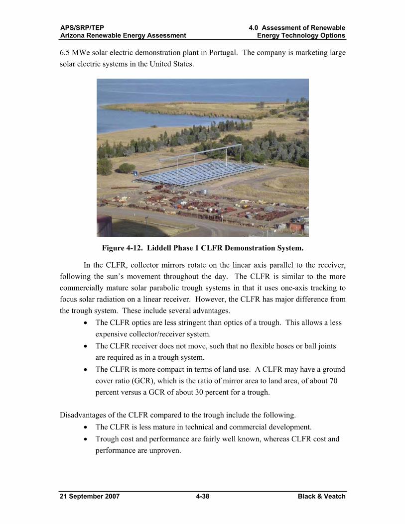
APS/SRP/TEPArizona Renewable Energy Assessment
4.0 Assessment of RenewableEnergy Technology Options
21 September 2007 4-38 Black & Veatch
6.5 MWe solar electric demonstration plant in Portugal. The company is marketing large solar electric systems in the United States.
Figure 4-12. Liddell Phase 1 CLFR Demonstration System.
In the CLFR, collector mirrors rotate on the linear axis parallel to the receiver, following the sun’s movement throughout the day. The CLFR is similar to the more commercially mature solar parabolic trough systems in that it uses one-axis tracking to focus solar radiation on a linear receiver. However, the CLFR has major difference from the trough system. These include several advantages.
The CLFR optics are less stringent than optics of a trough. This allows a less expensive collector/receiver system. The CLFR receiver does not move, such that no flexible hoses or ball joints are required as in a trough system. The CLFR is more compact in terms of land use. A CLFR may have a ground cover ratio (GCR), which is the ratio of mirror area to land area, of about 70 percent versus a GCR of about 30 percent for a trough.
Disadvantages of the CLFR compared to the trough include the following. The CLFR is less mature in technical and commercial development. Trough cost and performance are fairly well known, whereas CLFR cost and performance are unproven.
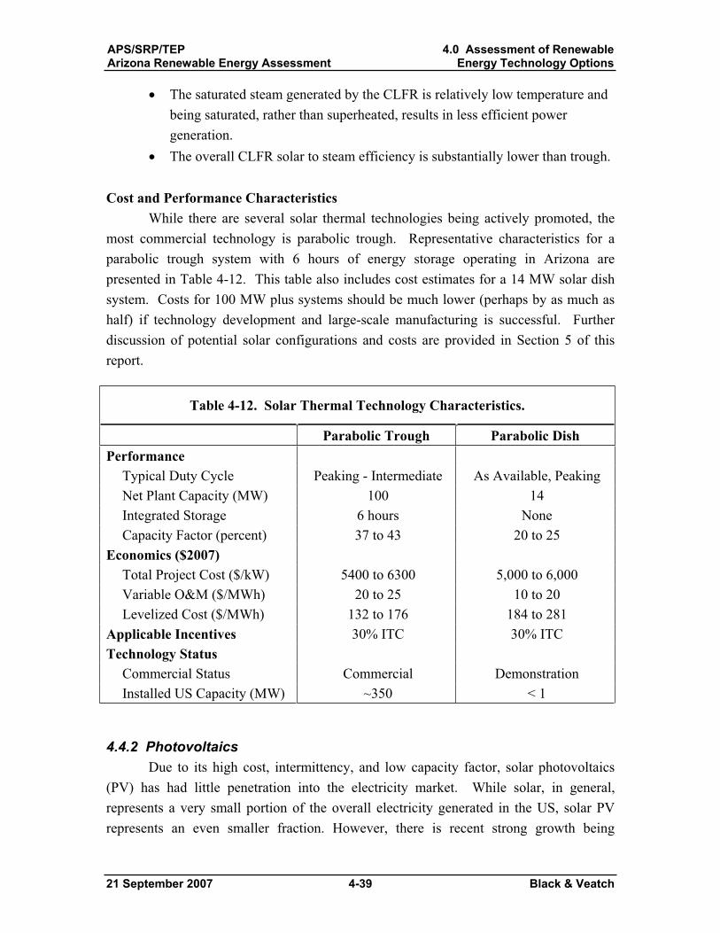
APS/SRP/TEPArizona Renewable Energy Assessment
4.0 Assessment of RenewableEnergy Technology Options
21 September 2007 4-39 Black & Veatch
The saturated steam generated by the CLFR is relatively low temperature and being saturated, rather than superheated, results in less efficient power generation.The overall CLFR solar to steam efficiency is substantially lower than trough.
Cost and Performance Characteristics While there are several solar thermal technologies being actively promoted, the
most commercial technology is parabolic trough. Representative characteristics for a parabolic trough system with 6 hours of energy storage operating in Arizona are presented in Table 4-12. This table also includes cost estimates for a 14 MW solar dish system. Costs for 100 MW plus systems should be much lower (perhaps by as much as half) if technology development and large-scale manufacturing is successful. Further discussion of potential solar configurations and costs are provided in Section 5 of this report.
Table 4-12. Solar Thermal Technology Characteristics.
Parabolic Trough Parabolic Dish Performance
Typical Duty Cycle Peaking - Intermediate As Available, Peaking Net Plant Capacity (MW) 100 14 Integrated Storage 6 hours None Capacity Factor (percent) 37 to 43 20 to 25
Economics ($2007) Total Project Cost ($/kW) 5400 to 6300 5,000 to 6,000 Variable O&M ($/MWh) 20 to 25 10 to 20 Levelized Cost ($/MWh) 132 to 176 184 to 281
Applicable Incentives 30% ITC 30% ITC Technology Status
Commercial Status Commercial Demonstration Installed US Capacity (MW) ~350 < 1
4.4.2 PhotovoltaicsDue to its high cost, intermittency, and low capacity factor, solar photovoltaics
(PV) has had little penetration into the electricity market. While solar, in general, represents a very small portion of the overall electricity generated in the US, solar PV represents an even smaller fraction. However, there is recent strong growth being
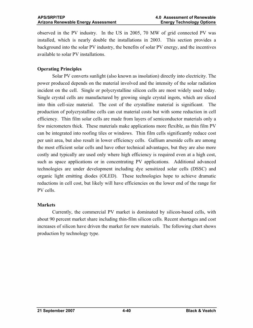
APS/SRP/TEPArizona Renewable Energy Assessment
4.0 Assessment of RenewableEnergy Technology Options
21 September 2007 4-40 Black & Veatch
observed in the PV industry. In the US in 2005, 70 MW of grid connected PV was installed, which is nearly double the installations in 2003. This section provides a background into the solar PV industry, the benefits of solar PV energy, and the incentives available to solar PV installations.
Operating Principles Solar PV converts sunlight (also known as insolation) directly into electricity. The
power produced depends on the material involved and the intensity of the solar radiation incident on the cell. Single or polycrystalline silicon cells are most widely used today. Single crystal cells are manufactured by growing single crystal ingots, which are sliced into thin cell-size material. The cost of the crystalline material is significant. The production of polycrystalline cells can cut material costs but with some reduction in cell efficiency. Thin film solar cells are made from layers of semiconductor materials only a few micrometers thick. These materials make applications more flexible, as thin film PV can be integrated into roofing tiles or windows. Thin film cells significantly reduce cost per unit area, but also result in lower efficiency cells. Gallium arsenide cells are among the most efficient solar cells and have other technical advantages, but they are also more costly and typically are used only where high efficiency is required even at a high cost, such as space applications or in concentrating PV applications. Additional advanced technologies are under development including dye sensitized solar cells (DSSC) and organic light emitting diodes (OLED). These technologies hope to achieve dramatic reductions in cell cost, but likely will have efficiencies on the lower end of the range for PV cells.
MarketsCurrently, the commercial PV market is dominated by silicon-based cells, with
about 90 percent market share including thin-film silicon cells. Recent shortages and cost increases of silicon have driven the market for new materials. The following chart shows production by technology type.
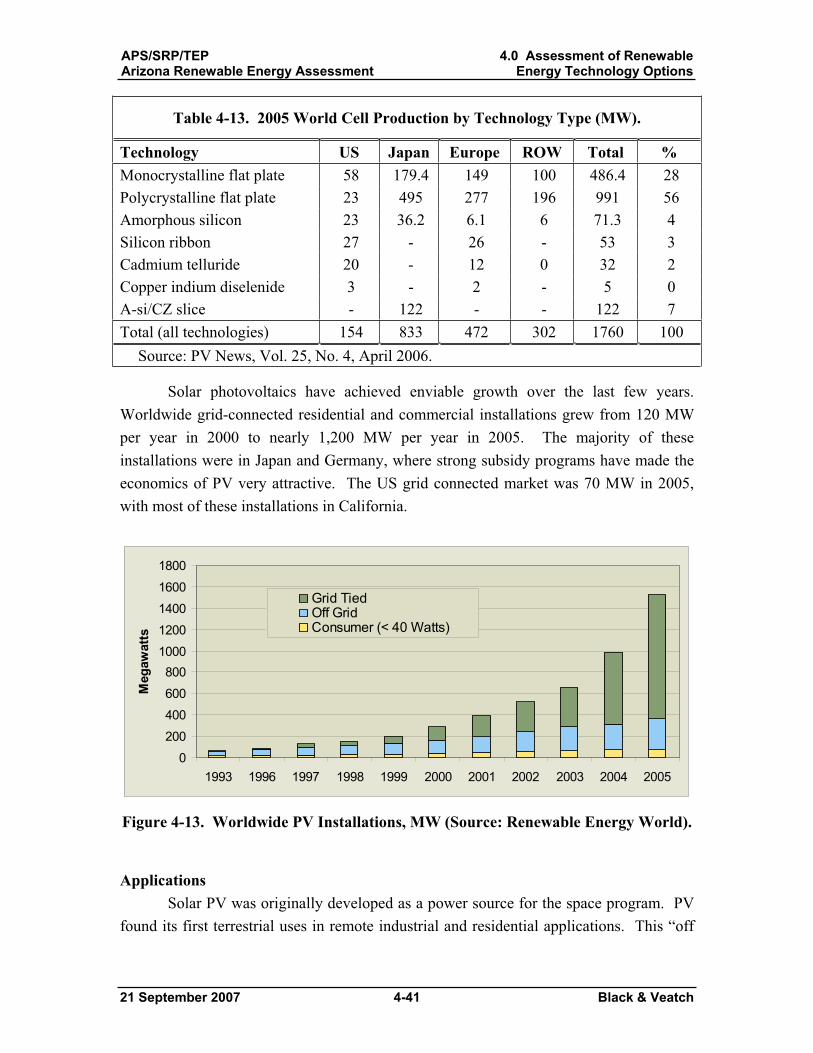
APS/SRP/TEPArizona Renewable Energy Assessment
4.0 Assessment of RenewableEnergy Technology Options
21 September 2007 4-41 Black & Veatch
Table 4-13. 2005 World Cell Production by Technology Type (MW).
Technology US Japan Europe ROW Total % Monocrystalline flat plate 58 179.4 149 100 486.4 28 Polycrystalline flat plate 23 495 277 196 991 56 Amorphous silicon 23 36.2 6.1 6 71.3 4 Silicon ribbon 27 - 26 - 53 3 Cadmium telluride 20 - 12 0 32 2 Copper indium diselenide 3 - 2 - 5 0 A-si/CZ slice - 122 - - 122 7 Total (all technologies) 154 833 472 302 1760 100
Source: PV News, Vol. 25, No. 4, April 2006.
Solar photovoltaics have achieved enviable growth over the last few years. Worldwide grid-connected residential and commercial installations grew from 120 MW per year in 2000 to nearly 1,200 MW per year in 2005. The majority of these installations were in Japan and Germany, where strong subsidy programs have made the economics of PV very attractive. The US grid connected market was 70 MW in 2005, with most of these installations in California.
0
200
400
600
8001000
1200
1400
1600
1800
1993 1996 1997 1998 1999 2000 2001 2002 2003 2004 2005
Meg
awat
ts
Grid TiedOff GridConsumer (< 40 Watts)
Figure 4-13. Worldwide PV Installations, MW (Source: Renewable Energy World).
Applications Solar PV was originally developed as a power source for the space program. PV
found its first terrestrial uses in remote industrial and residential applications. This “off
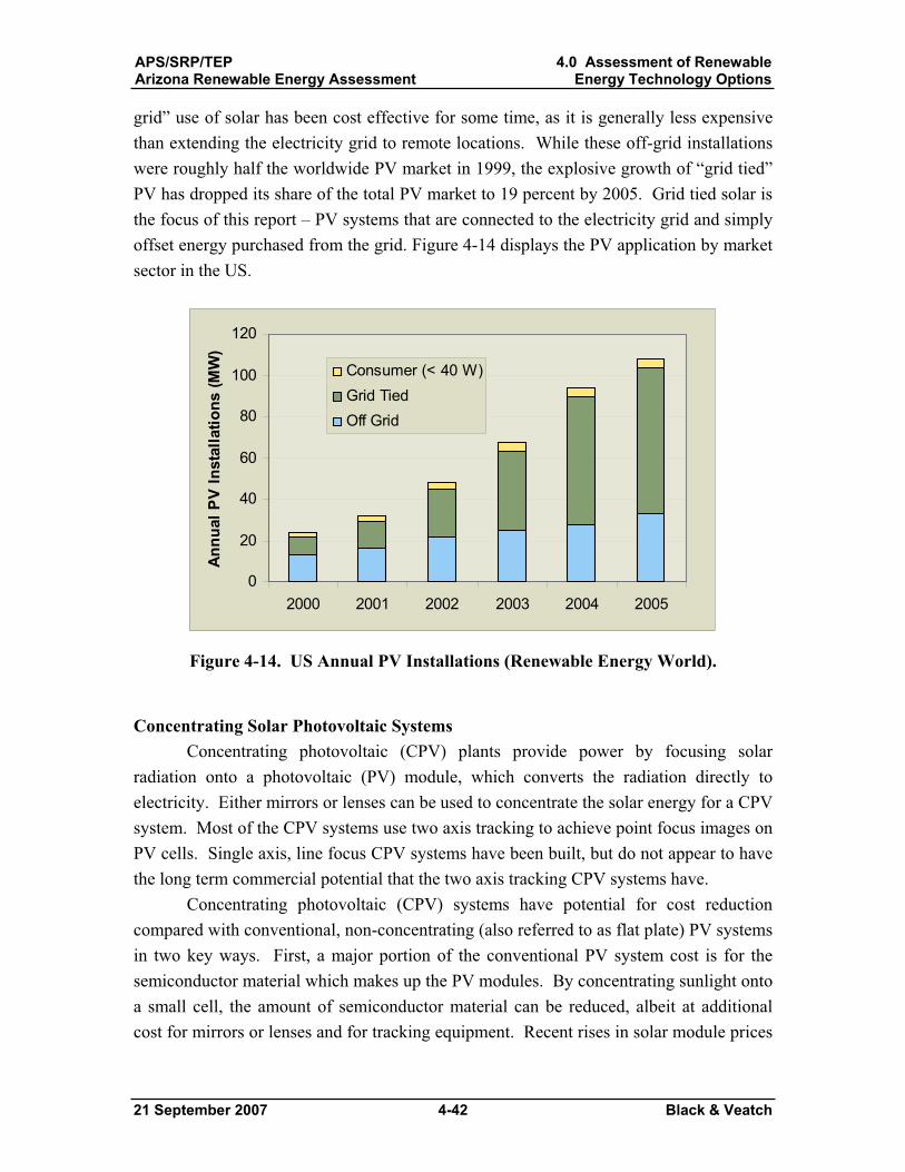
APS/SRP/TEPArizona Renewable Energy Assessment
4.0 Assessment of RenewableEnergy Technology Options
21 September 2007 4-42 Black & Veatch
grid” use of solar has been cost effective for some time, as it is generally less expensive than extending the electricity grid to remote locations. While these off-grid installations were roughly half the worldwide PV market in 1999, the explosive growth of “grid tied” PV has dropped its share of the total PV market to 19 percent by 2005. Grid tied solar is the focus of this report – PV systems that are connected to the electricity grid and simply offset energy purchased from the grid. Figure 4-14 displays the PV application by market sector in the US.
0
20
40
60
80
100
120
2000 2001 2002 2003 2004 2005
Annu
al P
V In
stal
latio
ns (M
W)
Consumer (< 40 W)Grid TiedOff Grid
Figure 4-14. US Annual PV Installations (Renewable Energy World).
Concentrating Solar Photovoltaic Systems Concentrating photovoltaic (CPV) plants provide power by focusing solar
radiation onto a photovoltaic (PV) module, which converts the radiation directly to electricity. Either mirrors or lenses can be used to concentrate the solar energy for a CPV system. Most of the CPV systems use two axis tracking to achieve point focus images on PV cells. Single axis, line focus CPV systems have been built, but do not appear to have the long term commercial potential that the two axis tracking CPV systems have.
Concentrating photovoltaic (CPV) systems have potential for cost reduction compared with conventional, non-concentrating (also referred to as flat plate) PV systems in two key ways. First, a major portion of the conventional PV system cost is for the semiconductor material which makes up the PV modules. By concentrating sunlight onto a small cell, the amount of semiconductor material can be reduced, albeit at additional cost for mirrors or lenses and for tracking equipment. Recent rises in solar module prices
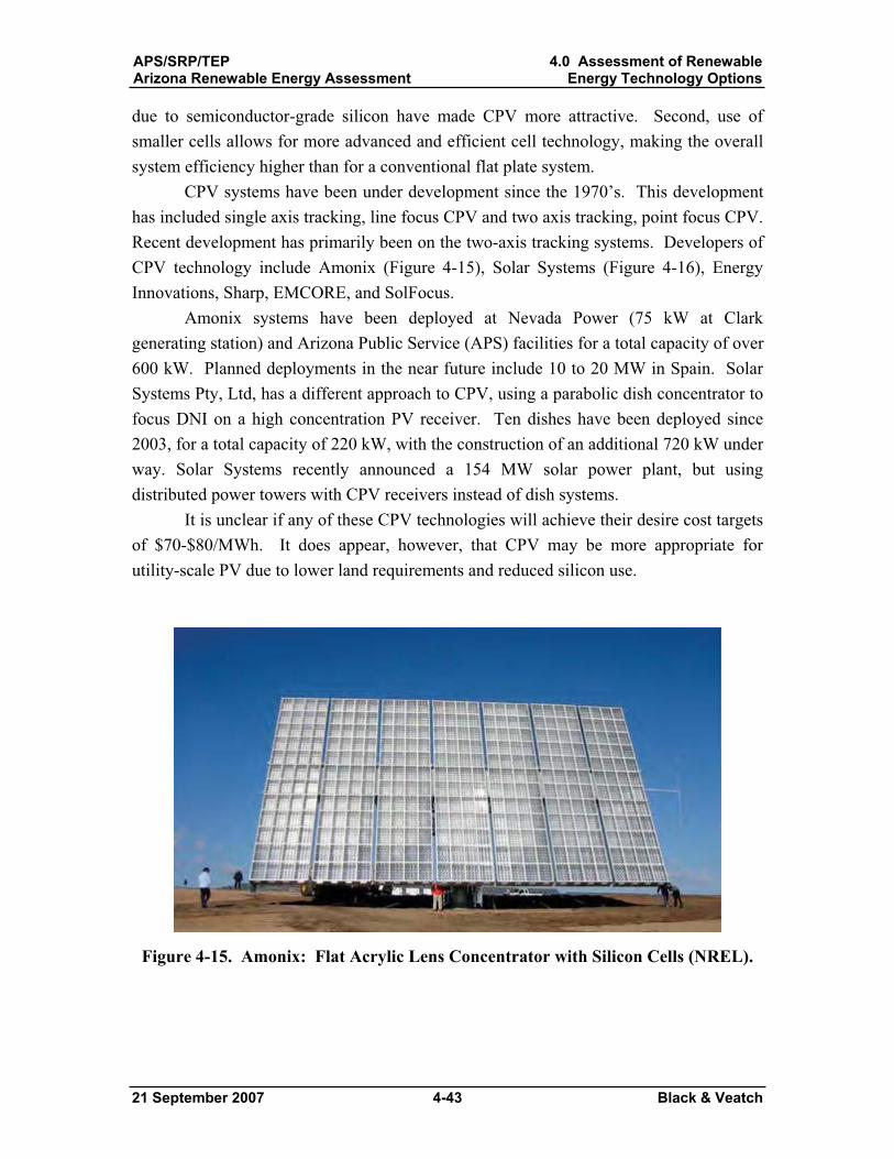
APS/SRP/TEPArizona Renewable Energy Assessment
4.0 Assessment of RenewableEnergy Technology Options
21 September 2007 4-43 Black & Veatch
due to semiconductor-grade silicon have made CPV more attractive. Second, use of smaller cells allows for more advanced and efficient cell technology, making the overall system efficiency higher than for a conventional flat plate system.
CPV systems have been under development since the 1970’s. This development has included single axis tracking, line focus CPV and two axis tracking, point focus CPV.Recent development has primarily been on the two-axis tracking systems. Developers of CPV technology include Amonix (Figure 4-15), Solar Systems (Figure 4-16), Energy Innovations, Sharp, EMCORE, and SolFocus.
Amonix systems have been deployed at Nevada Power (75 kW at Clark generating station) and Arizona Public Service (APS) facilities for a total capacity of over 600 kW. Planned deployments in the near future include 10 to 20 MW in Spain. Solar Systems Pty, Ltd, has a different approach to CPV, using a parabolic dish concentrator to focus DNI on a high concentration PV receiver. Ten dishes have been deployed since 2003, for a total capacity of 220 kW, with the construction of an additional 720 kW under way. Solar Systems recently announced a 154 MW solar power plant, but using distributed power towers with CPV receivers instead of dish systems.
It is unclear if any of these CPV technologies will achieve their desire cost targets of $70-$80/MWh. It does appear, however, that CPV may be more appropriate for utility-scale PV due to lower land requirements and reduced silicon use.
Figure 4-15. Amonix: Flat Acrylic Lens Concentrator with Silicon Cells (NREL).
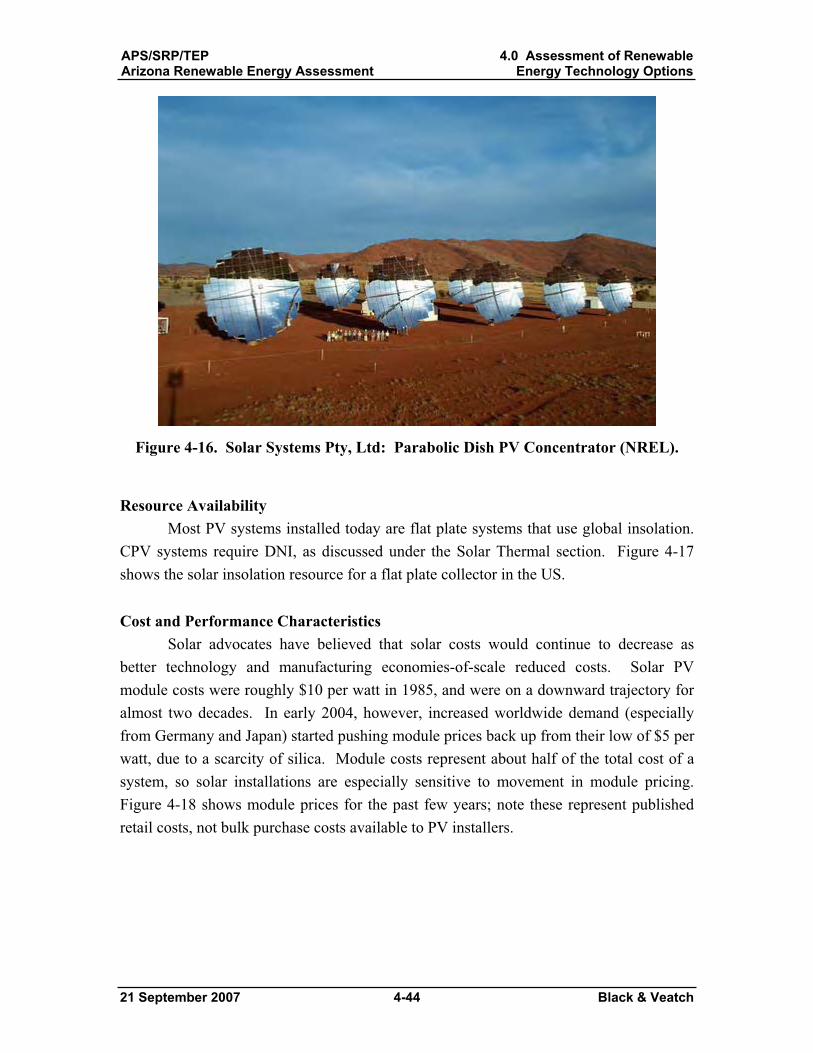
APS/SRP/TEPArizona Renewable Energy Assessment
4.0 Assessment of RenewableEnergy Technology Options
21 September 2007 4-44 Black & Veatch
Figure 4-16. Solar Systems Pty, Ltd: Parabolic Dish PV Concentrator (NREL).
Resource Availability Most PV systems installed today are flat plate systems that use global insolation.
CPV systems require DNI, as discussed under the Solar Thermal section. Figure 4-17shows the solar insolation resource for a flat plate collector in the US.
Cost and Performance Characteristics Solar advocates have believed that solar costs would continue to decrease as
better technology and manufacturing economies-of-scale reduced costs. Solar PV module costs were roughly $10 per watt in 1985, and were on a downward trajectory for almost two decades. In early 2004, however, increased worldwide demand (especially from Germany and Japan) started pushing module prices back up from their low of $5 per watt, due to a scarcity of silica. Module costs represent about half of the total cost of a system, so solar installations are especially sensitive to movement in module pricing. Figure 4-18 shows module prices for the past few years; note these represent published retail costs, not bulk purchase costs available to PV installers.
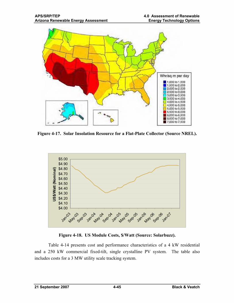
APS/SRP/TEPArizona Renewable Energy Assessment
4.0 Assessment of RenewableEnergy Technology Options
21 September 2007 4-45 Black & Veatch
Figure 4-17. Solar Insolation Resource for a Flat-Plate Collector (Source NREL).
$4.00$4.10$4.20$4.30$4.40$4.50$4.60$4.70$4.80$4.90$5.00
Jan-0
3
May-03
Sep-03
Jan-0
4
May-04
Sep-04
Jan-0
5
May-05
Sep-05
Jan-0
6
May-06
Sep-06
Jan-0
7
US$/
Wat
t (No
min
al)
Figure 4-18. US Module Costs, $/Watt (Source: Solarbuzz).
Table 4-14 presents cost and performance characteristics of a 4 kW residential and a 250 kW commercial fixed-tilt, single crystalline PV system. The table also includes costs for a 3 MW utility scale tracking system.
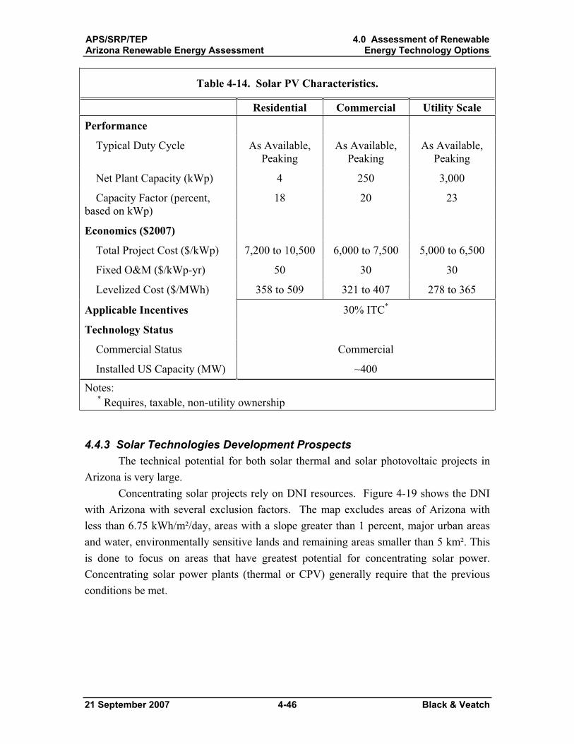
APS/SRP/TEPArizona Renewable Energy Assessment
4.0 Assessment of RenewableEnergy Technology Options
21 September 2007 4-46 Black & Veatch
Table 4-14. Solar PV Characteristics.
Residential Commercial Utility Scale Performance
Typical Duty Cycle As Available, Peaking
As Available, Peaking
As Available, Peaking
Net Plant Capacity (kWp) 4 250 3,000
Capacity Factor (percent, based on kWp)
18 20 23
Economics ($2007)
Total Project Cost ($/kWp) 7,200 to 10,500 6,000 to 7,500 5,000 to 6,500
Fixed O&M ($/kWp-yr) 50 30 30
Levelized Cost ($/MWh) 358 to 509 321 to 407 278 to 365
Applicable Incentives 30% ITC*
Technology Status
Commercial Status Commercial
Installed US Capacity (MW) ~400
Notes:* Requires, taxable, non-utility ownership
4.4.3 Solar Technologies Development Prospects The technical potential for both solar thermal and solar photovoltaic projects in
Arizona is very large.Concentrating solar projects rely on DNI resources. Figure 4-19 shows the DNI
with Arizona with several exclusion factors. The map excludes areas of Arizona with less than 6.75 kWh/m²/day, areas with a slope greater than 1 percent, major urban areas and water, environmentally sensitive lands and remaining areas smaller than 5 km². This is done to focus on areas that have greatest potential for concentrating solar power. Concentrating solar power plants (thermal or CPV) generally require that the previous conditions be met.
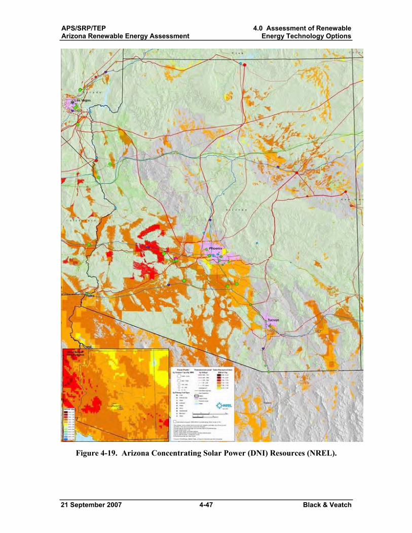
APS/SRP/TEPArizona Renewable Energy Assessment
4.0 Assessment of RenewableEnergy Technology Options
21 September 2007 4-47 Black & Veatch
Figure 4-19. Arizona Concentrating Solar Power (DNI) Resources (NREL).
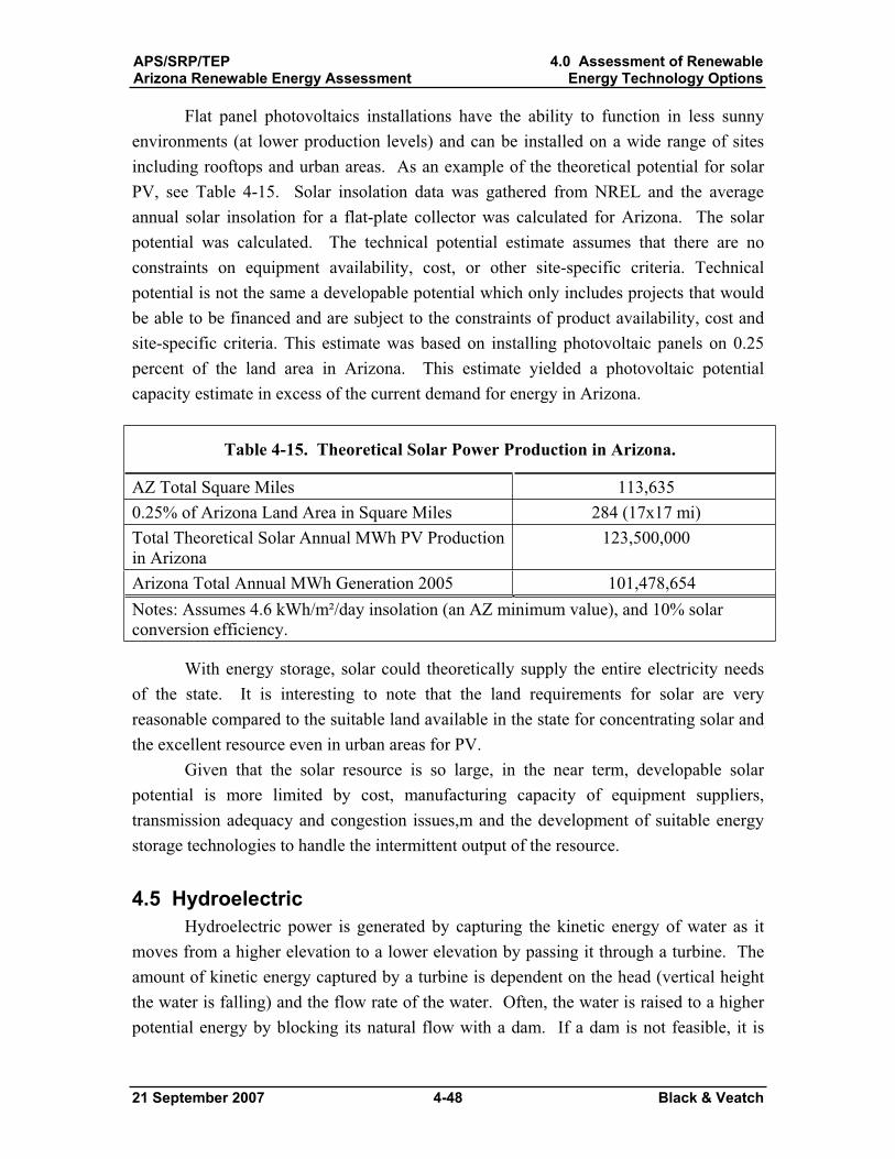
APS/SRP/TEPArizona Renewable Energy Assessment
4.0 Assessment of RenewableEnergy Technology Options
21 September 2007 4-48 Black & Veatch
Flat panel photovoltaics installations have the ability to function in less sunny environments (at lower production levels) and can be installed on a wide range of sites including rooftops and urban areas. As an example of the theoretical potential for solar PV, see Table 4-15. Solar insolation data was gathered from NREL and the average annual solar insolation for a flat-plate collector was calculated for Arizona. The solar potential was calculated. The technical potential estimate assumes that there are no constraints on equipment availability, cost, or other site-specific criteria. Technical potential is not the same a developable potential which only includes projects that would be able to be financed and are subject to the constraints of product availability, cost and site-specific criteria. This estimate was based on installing photovoltaic panels on 0.25 percent of the land area in Arizona. This estimate yielded a photovoltaic potential capacity estimate in excess of the current demand for energy in Arizona.
Table 4-15. Theoretical Solar Power Production in Arizona.
AZ Total Square Miles 113,635 0.25% of Arizona Land Area in Square Miles 284 (17x17 mi) Total Theoretical Solar Annual MWh PV Production in Arizona
123,500,000
Arizona Total Annual MWh Generation 2005 101,478,654 Notes: Assumes 4.6 kWh/m²/day insolation (an AZ minimum value), and 10% solar conversion efficiency.
With energy storage, solar could theoretically supply the entire electricity needs of the state. It is interesting to note that the land requirements for solar are very reasonable compared to the suitable land available in the state for concentrating solar and the excellent resource even in urban areas for PV.
Given that the solar resource is so large, in the near term, developable solar potential is more limited by cost, manufacturing capacity of equipment suppliers, transmission adequacy and congestion issues,m and the development of suitable energy storage technologies to handle the intermittent output of the resource.
4.5 Hydroelectric Hydroelectric power is generated by capturing the kinetic energy of water as it
moves from a higher elevation to a lower elevation by passing it through a turbine. The amount of kinetic energy captured by a turbine is dependent on the head (vertical height the water is falling) and the flow rate of the water. Often, the water is raised to a higher potential energy by blocking its natural flow with a dam. If a dam is not feasible, it is
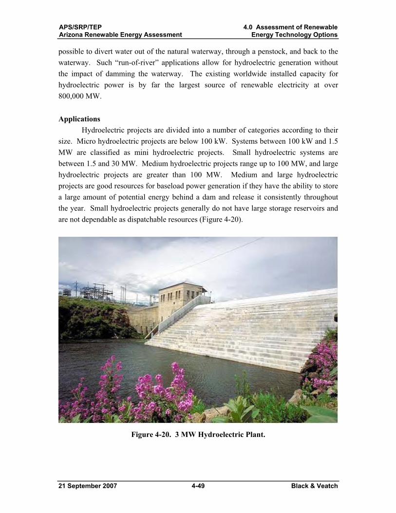
APS/SRP/TEPArizona Renewable Energy Assessment
4.0 Assessment of RenewableEnergy Technology Options
21 September 2007 4-49 Black & Veatch
possible to divert water out of the natural waterway, through a penstock, and back to the waterway. Such “run-of-river” applications allow for hydroelectric generation without the impact of damming the waterway. The existing worldwide installed capacity for hydroelectric power is by far the largest source of renewable electricity at over 800,000 MW.
Applications Hydroelectric projects are divided into a number of categories according to their
size. Micro hydroelectric projects are below 100 kW. Systems between 100 kW and 1.5 MW are classified as mini hydroelectric projects. Small hydroelectric systems are between 1.5 and 30 MW. Medium hydroelectric projects range up to 100 MW, and large hydroelectric projects are greater than 100 MW. Medium and large hydroelectric projects are good resources for baseload power generation if they have the ability to store a large amount of potential energy behind a dam and release it consistently throughout the year. Small hydroelectric projects generally do not have large storage reservoirs and are not dependable as dispatchable resources (Figure 4-20).
Figure 4-20. 3 MW Hydroelectric Plant.
APS/SRP/TEPArizona Renewable Energy Assessment
4.0 Assessment of RenewableEnergy Technology Options
21 September 2007 4-50 Black & Veatch
Resource Availability A hydroelectric resource can be defined as any flow of water that can be used to
capture the kinetic energy. Projects that store large amounts of water behind a dam can regulate the release of water through turbines and generate electricity regardless of the season. These facilities can generally serve base loads. Run-of-river projects do not impound the water, but instead divert a part or all of the current through a turbine to generate electricity. At run-of-river projects, power generation varies with seasonal flows and can sometimes help serve summer peak loads.
All hydroelectric projects are susceptible to drought. In fact, the variability in hydroelectric output is rather large, even when compared to other renewable resources. The aggregate capacity factor for all hydroelectric plants in the United States has ranged from a high of 47 percent to a low of 31 percent.
Cost and Performance Characteristics Hydroelectric generation is regarded as a mature technology that is unlikely to
advance. Turbine efficiency and costs have remained somewhat stable, but construction techniques and costs continue to change. Capital costs are highly dependent onsite characteristics and vary widely. Table 4-16 provides ranges for performance and cost estimates for hydroelectric projects for two categories: new projects at undeveloped sites and additions or upgrades to hydroelectric projects at existing sites. These values are for representative comparison purposes only. Capacity factors are highly resource dependent and can range from 10 to more than 90 percent. Capital costs also vary widely with site conditions.
Environmental Impacts The damming of rivers for small- and large-scale hydroelectric applications may
have significant environmental impacts. One major issue involves the migration of fish and disruption of spawning habits. For dam projects, one of the common solutions to this problem is the construction of “fish ladders” to aid the fish in bypassing the dam when they swim upstream to spawn.
A second issue involves flooding existing valleys that often contain wilderness areas, residential areas, or archeologically significant remains. There are also concerns about the consequences of disrupting the natural flow of water downstream and disrupting the natural course of nature.
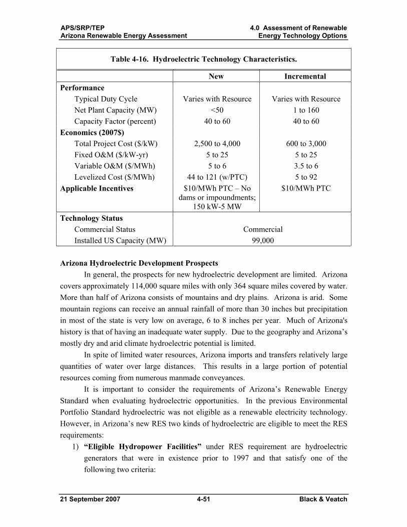
APS/SRP/TEPArizona Renewable Energy Assessment
4.0 Assessment of RenewableEnergy Technology Options
21 September 2007 4-51 Black & Veatch
Table 4-16. Hydroelectric Technology Characteristics.
New Incremental Performance
Typical Duty Cycle Varies with Resource Varies with Resource Net Plant Capacity (MW) <50 1 to 160 Capacity Factor (percent) 40 to 60 40 to 60
Economics (2007$) Total Project Cost ($/kW) 2,500 to 4,000 600 to 3,000 Fixed O&M ($/kW-yr) 5 to 25 5 to 25 Variable O&M ($/MWh) 5 to 6 3.5 to 6 Levelized Cost ($/MWh) 44 to 121 (w/PTC) 5 to 92
Applicable Incentives $10/MWh PTC – No dams or impoundments;
150 kW-5 MW
$10/MWh PTC
Technology Status Commercial Status Commercial Installed US Capacity (MW) 99,000
Arizona Hydroelectric Development Prospects In general, the prospects for new hydroelectric development are limited. Arizona
covers approximately 114,000 square miles with only 364 square miles covered by water. More than half of Arizona consists of mountains and dry plains. Arizona is arid. Some mountain regions can receive an annual rainfall of more than 30 inches but precipitation in most of the state is very low on average, 6 to 8 inches per year. Much of Arizona's history is that of having an inadequate water supply. Due to the geography and Arizona’s mostly dry and arid climate hydroelectric potential is limited.
In spite of limited water resources, Arizona imports and transfers relatively large quantities of water over large distances. This results in a large portion of potential resources coming from numerous manmade conveyances.
It is important to consider the requirements of Arizona’s Renewable Energy Standard when evaluating hydroelectric opportunities. In the previous Environmental Portfolio Standard hydroelectric was not eligible as a renewable electricity technology. However, in Arizona’s new RES two kinds of hydroelectric are eligible to meet the RES requirements:
1) “Eligible Hydropower Facilities” under RES requirement are hydroelectric generators that were in existence prior to 1997 and that satisfy one of the following two criteria:
APS/SRP/TEPArizona Renewable Energy Assessment
4.0 Assessment of RenewableEnergy Technology Options
21 September 2007 4-52 Black & Veatch
a) New Increased Capacity of Existing Hydroelectric Facilities: A hydroelectric facility that increases capacity due to improved technological or operational efficiencies or operational improvements resulting from improved or modified turbine design, improved or modified wicket gate assembly design, improved hydrological flow conditions, improved generator windings, improved electrical excitation systems, increases in transformation capacity, and improved system control and operating limit modifications. The electricity kWh that are eligible to meet the Annual Renewable Energy Requirements shall be limited to the new, incremental kWh output resulting from the capacity increase that is delivered to Arizona customers to meet the Annual Renewable Energy Requirement.
b) Generation from pre-1997 hydroelectric facilities that is used to firm or regulate the output of other eligible, intermittent renewable resources: The electricity kWh that are eligible to meet the Annual Renewable Energy Requirements shall be limited to the kWh actually generated to firm or regulate the output of eligible intermittent Renewable Energy Resources and that are delivered to Arizona customers to meet the Annual Renewable Energy Requirements.
2) “New Hydropower Generator of 10 MW or Less” under RES requirement is a generator, installed after January 1 2006 that produces 10 MW or less and is either: a) A low-head, micro hydroelectric run-of-the-river system that does not require
any new damming of the flow of the stream; or b) An existing dam that adds power generation equipment without requiring a
new dam, diversion structures, or a change in water flow that will adversely impact fish, wildlife, or water quality; or
c) Generation using canals or other irrigation systems.
Other hydroelectric resources not regulated by RES Rules, such as the Salt River Project, are generally considered a renewable resource by many states if less than 30 MW.
There are 21 existing dam sites in Arizona with additional hydroelectric potential identified by the federal government. The U.S. Department of Energy Idaho National Engineering and Environmental Laboratory (INL) provides this information as part of the National Energy Strategy. These sites consist of 13 undeveloped sites with no developed impoundment or diversion structure, 6 developed sites with some kind of impoundment or diversion structure, and 2 sites with developed hydroelectric generation but where the
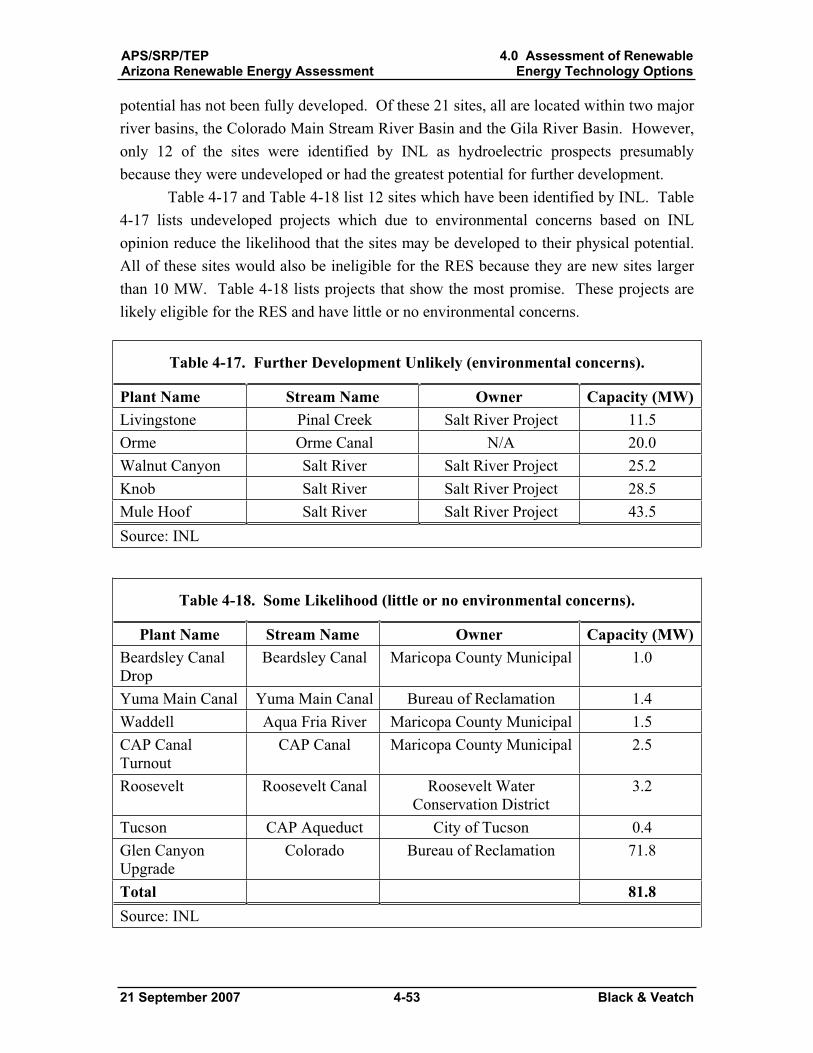
APS/SRP/TEPArizona Renewable Energy Assessment
4.0 Assessment of RenewableEnergy Technology Options
21 September 2007 4-53 Black & Veatch
potential has not been fully developed. Of these 21 sites, all are located within two major river basins, the Colorado Main Stream River Basin and the Gila River Basin. However, only 12 of the sites were identified by INL as hydroelectric prospects presumably because they were undeveloped or had the greatest potential for further development.
Table 4-17 and Table 4-18 list 12 sites which have been identified by INL. Table 4-17 lists undeveloped projects which due to environmental concerns based on INL opinion reduce the likelihood that the sites may be developed to their physical potential. All of these sites would also be ineligible for the RES because they are new sites larger than 10 MW. Table 4-18 lists projects that show the most promise. These projects are likely eligible for the RES and have little or no environmental concerns.
Table 4-17. Further Development Unlikely (environmental concerns).
Plant Name Stream Name Owner Capacity (MW)Livingstone Pinal Creek Salt River Project 11.5 Orme Orme Canal N/A 20.0 Walnut Canyon Salt River Salt River Project 25.2 Knob Salt River Salt River Project 28.5 Mule Hoof Salt River Salt River Project 43.5 Source: INL
Table 4-18. Some Likelihood (little or no environmental concerns).
Plant Name Stream Name Owner Capacity (MW)Beardsley Canal Drop
Beardsley Canal Maricopa County Municipal 1.0
Yuma Main Canal Yuma Main Canal Bureau of Reclamation 1.4 Waddell Aqua Fria River Maricopa County Municipal 1.5 CAP Canal Turnout
CAP Canal Maricopa County Municipal 2.5
Roosevelt Roosevelt Canal Roosevelt Water Conservation District
3.2
Tucson CAP Aqueduct City of Tucson 0.4 Glen Canyon Upgrade
Colorado Bureau of Reclamation 71.8
Total 81.8Source: INL
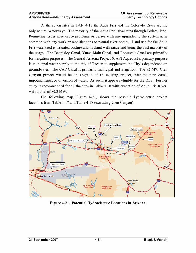
APS/SRP/TEPArizona Renewable Energy Assessment
4.0 Assessment of RenewableEnergy Technology Options
21 September 2007 4-54 Black & Veatch
Of the seven sites in Table 4-18 the Aqua Fria and the Colorado River are the only natural waterways. The majority of the Aqua Fria River runs through Federal land. Permitting issues may cause problems or delays with any upgrades to the system as is common with any work or modifications to natural river bodies. Land use for the Aqua Fria watershed is irrigated pasture and hayland with rangeland being the vast majority of the usage. The Beardsley Canal, Yuma Main Canal, and Roosevelt Canal are primarily for irrigation purposes. The Central Arizona Project (CAP) Aqueduct’s primary purpose is municipal water supply to the city of Tucson to supplement the City’s dependence on groundwater. The CAP Canal is primarily municipal and irrigation. The 72 MW Glen Canyon project would be an upgrade of an existing project, with no new dams, impoundments, or diversion of water. As such, it appears eligible for the RES. Further study is recommended for all the sites in Table 4-18 with exception of Aqua Fria River, with a total of 80.3 MW.
The following map, Figure 4-21, shows the possible hydroelectric project locations from Table 4-17 and Table 4-18 (excluding Glen Canyon):
Figure 4-21. Potential Hydroelectric Locations in Arizona.
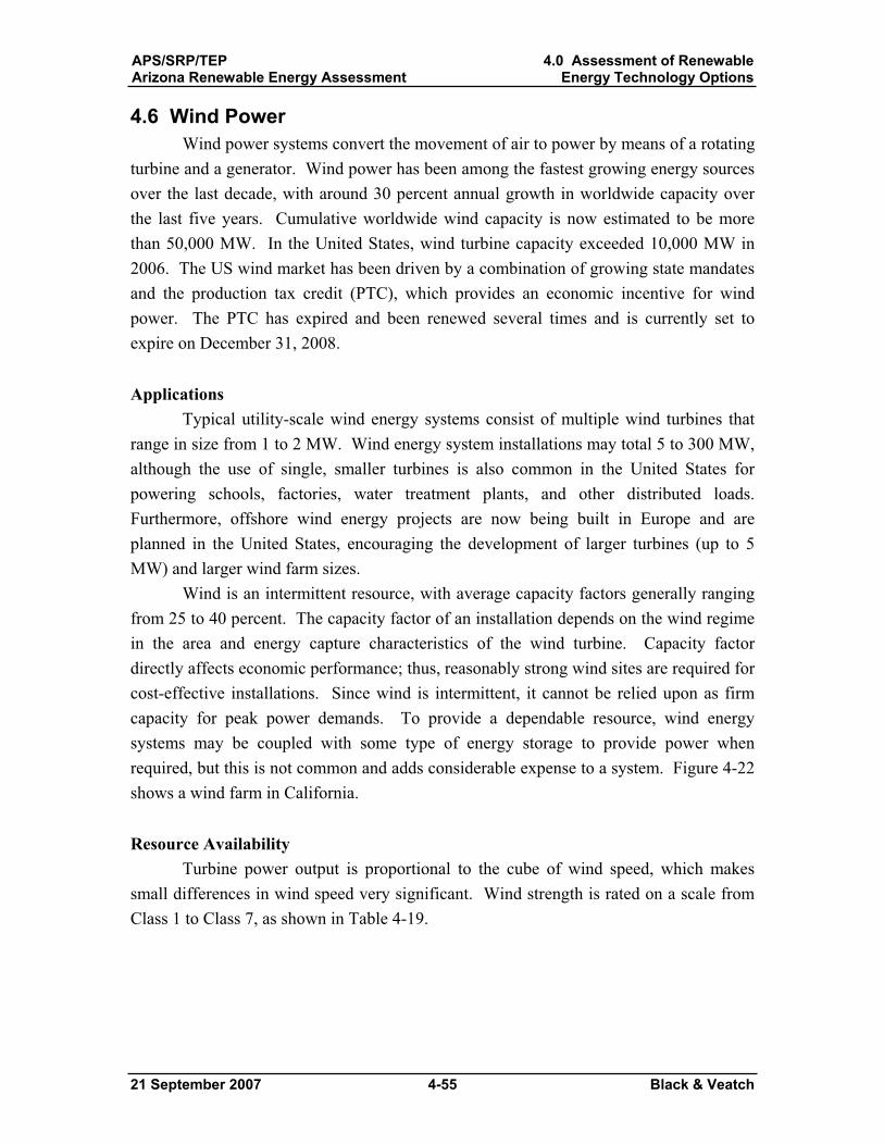
APS/SRP/TEPArizona Renewable Energy Assessment
4.0 Assessment of RenewableEnergy Technology Options
21 September 2007 4-55 Black & Veatch
4.6 Wind Power Wind power systems convert the movement of air to power by means of a rotating
turbine and a generator. Wind power has been among the fastest growing energy sources over the last decade, with around 30 percent annual growth in worldwide capacity over the last five years. Cumulative worldwide wind capacity is now estimated to be more than 50,000 MW. In the United States, wind turbine capacity exceeded 10,000 MW in 2006. The US wind market has been driven by a combination of growing state mandates and the production tax credit (PTC), which provides an economic incentive for wind power. The PTC has expired and been renewed several times and is currently set to expire on December 31, 2008.
Applications Typical utility-scale wind energy systems consist of multiple wind turbines that
range in size from 1 to 2 MW. Wind energy system installations may total 5 to 300 MW, although the use of single, smaller turbines is also common in the United States for powering schools, factories, water treatment plants, and other distributed loads. Furthermore, offshore wind energy projects are now being built in Europe and are planned in the United States, encouraging the development of larger turbines (up to 5 MW) and larger wind farm sizes.
Wind is an intermittent resource, with average capacity factors generally ranging from 25 to 40 percent. The capacity factor of an installation depends on the wind regime in the area and energy capture characteristics of the wind turbine. Capacity factor directly affects economic performance; thus, reasonably strong wind sites are required for cost-effective installations. Since wind is intermittent, it cannot be relied upon as firm capacity for peak power demands. To provide a dependable resource, wind energy systems may be coupled with some type of energy storage to provide power when required, but this is not common and adds considerable expense to a system. Figure 4-22shows a wind farm in California.
Resource Availability Turbine power output is proportional to the cube of wind speed, which makes
small differences in wind speed very significant. Wind strength is rated on a scale from Class 1 to Class 7, as shown in Table 4-19.
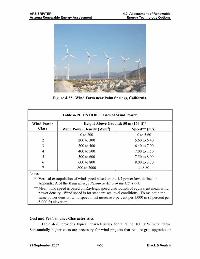
APS/SRP/TEPArizona Renewable Energy Assessment
4.0 Assessment of RenewableEnergy Technology Options
21 September 2007 4-56 Black & Veatch
Figure 4-22. Wind Farm near Palm Springs, California.
Table 4-19. US DOE Classes of Wind Power.
Height Above Ground: 50 m (164 ft)* Wind Power Class Wind Power Density (W/m2) Speed** (m/s)
1 0 to 200 0 to 5.60 2 200 to 300 5.60 to 6.40 3 300 to 400 6.40 to 7.00 4 400 to 500 7.00 to 7.50 5 500 to 600 7.50 to 8.00 6 600 to 800 8.00 to 8.80 7 800 to 2000 8.80
Notes:* Vertical extrapolation of wind speed based on the 1/7 power law, defined in
Appendix A of the Wind Energy Resource Atlas of the US, 1991.** Mean wind speed is based on Rayleigh speed distribution of equivalent mean wind
power density. Wind speed is for standard sea level conditions. To maintain the same power density, wind speed must increase 3 percent per 1,000 m (5 percent per 5,000 ft) elevation.
Cost and Performance Characteristics Table 4-20 provides typical characteristics for a 50 to 100 MW wind farm.
Substantially higher costs are necessary for wind projects that require grid upgrades or
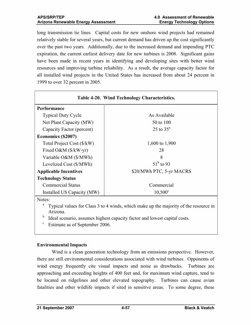
APS/SRP/TEPArizona Renewable Energy Assessment
4.0 Assessment of RenewableEnergy Technology Options
21 September 2007 4-57 Black & Veatch
long transmission tie lines. Capital costs for new onshore wind projects had remained relatively stable for several years, but current demand has driven up the cost significantly over the past two years. Additionally, due to the increased demand and impending PTC expiration, the current earliest delivery date for new turbines is 2008. Significant gains have been made in recent years in identifying and developing sites with better wind resources and improving turbine reliability. As a result, the average capacity factor for all installed wind projects in the United States has increased from about 24 percent in 1999 to over 32 percent in 2005.
Table 4-20. Wind Technology Characteristics.
PerformanceTypical Duty Cycle As Available Net Plant Capacity (MW) 50 to 100 Capacity Factor (percent) 25 to 35a
Economics ($2007) Total Project Cost ($/kW) 1,600 to 1,900 Fixed O&M ($/kW-yr) 28 Variable O&M ($/MWh) 8 Levelized Cost ($/MWh) 51b to 93
Applicable Incentives $20/MWh PTC, 5-yr MACRS Technology Status
Commercial Status Commercial Installed US Capacity (MW) 10,500c
Notes:a Typical values for Class 3 to 4 winds, which make up the majority of the resource in
Arizona.b Ideal scenario, assumes highest capacity factor and lowest capital costs. c Estimate as of September 2006.
Environmental Impacts Wind is a clean generation technology from an emissions perspective. However,
there are still environmental considerations associated with wind turbines. Opponents of wind energy frequently cite visual impacts and noise as drawbacks. Turbines are approaching and exceeding heights of 400 feet and, for maximum wind capture, tend to be located on ridgelines and other elevated topography. Turbines can cause avian fatalities and other wildlife impacts if sited in sensitive areas. To some degree, these
APS/SRP/TEPArizona Renewable Energy Assessment
4.0 Assessment of RenewableEnergy Technology Options
21 September 2007 4-58 Black & Veatch
issues can be partially mitigated through proper siting, environmental review, and the involvement of the public during the planning process.
Arizona Wind Potential Arizona has relatively large wind potential, although most of it is lower quality
resources. Much of the wind resource in Arizona is considered to be Class 2 or less, which is generally considered to be non-economic. There are fairly large areas of Class 3 winds, which are considered marginal wind resources. These are in a long line that passes near Flagstaff and continues to the eastern part of the state. Higher wind resources are predicted to exist along ridgelines as well. The map in Figure 4-23 shows the Class 3 and above wind resources in Arizona.
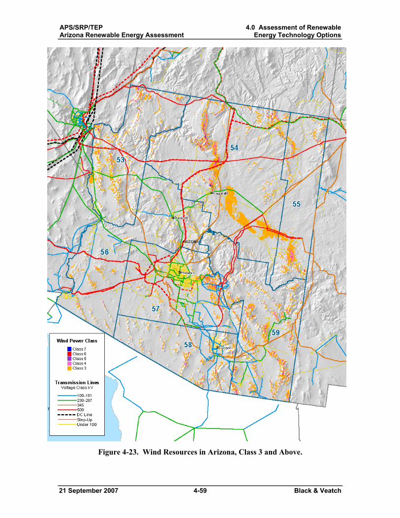
APS/SRP/TEPArizona Renewable Energy Assessment
4.0 Assessment of RenewableEnergy Technology Options
21 September 2007 4-59 Black & Veatch
Figure 4-23. Wind Resources in Arizona, Class 3 and Above.
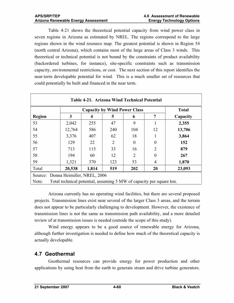
APS/SRP/TEPArizona Renewable Energy Assessment
4.0 Assessment of RenewableEnergy Technology Options
21 September 2007 4-60 Black & Veatch
Table 4-21 shows the theoretical potential capacity from wind power class in seven regions in Arizona as estimated by NREL. The regions correspond to the large regions shown in the wind resource map. The greatest potential is shown in Region 54 (north central Arizona), which contains most of the large areas of Class 3 winds. This theoretical or technical potential is not bound by the constraints of product availability(backordered turbines, for instance), site-specific constraints such as transmission capacity, environmental restrictions, or cost. The next section of this report identifies the near-term developable potential for wind. This is a much smaller set of resources that could potentially be built and financed in the near term.
Table 4-21. Arizona Wind Technical Potential
Capacity by Wind Power Class Total Region 3 4 5 6 7 Capacity 53 2,042 255 47 9 1 2,35554 12,764 586 240 104 12 13,70655 3,376 407 62 18 1 3,86456 129 22 2 0 0 15257 713 115 33 16 2 87958 194 60 12 2 0 26759 1,321 370 123 53 4 1,870Total 20,538 1,814 519 202 20 23,093 Source: Donna Heimiller, NREL, 2006 Note: Total technical potential, assuming 5 MW of capacity per square km.
Arizona currently has no operating wind facilities, but there are several proposed projects. Transmission lines exist near several of the larger Class 3 areas, and the terrain does not appear to be particularly challenging to development. However, the existence of transmission lines is not the same as transmission path availability, and a more detailed review of at transmission issues is needed (outside the scope of this study).
Wind energy appears to be a good source of renewable energy for Arizona, although further investigation is needed to define how much of the theoretical capacity is actually developable.
4.7 Geothermal Geothermal resources can provide energy for power production and other
applications by using heat from the earth to generate steam and drive turbine generators.
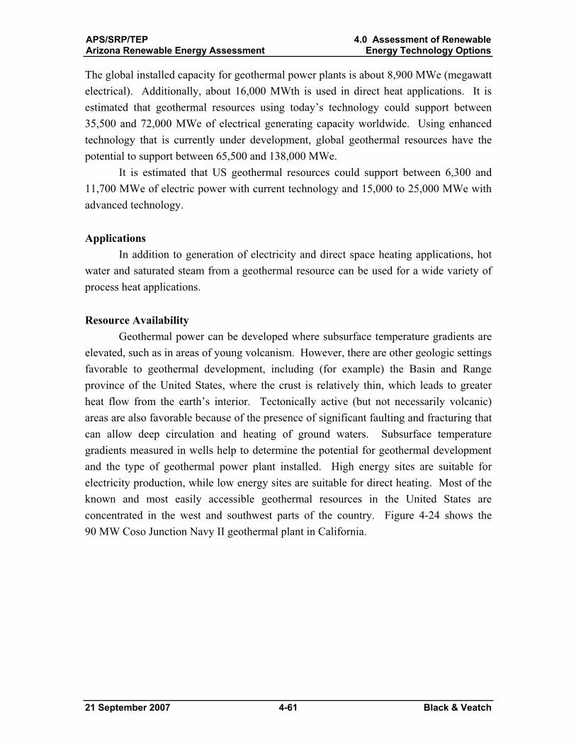
APS/SRP/TEPArizona Renewable Energy Assessment
4.0 Assessment of RenewableEnergy Technology Options
21 September 2007 4-61 Black & Veatch
The global installed capacity for geothermal power plants is about 8,900 MWe (megawatt electrical). Additionally, about 16,000 MWth is used in direct heat applications. It is estimated that geothermal resources using today’s technology could support between 35,500 and 72,000 MWe of electrical generating capacity worldwide. Using enhanced technology that is currently under development, global geothermal resources have the potential to support between 65,500 and 138,000 MWe.
It is estimated that US geothermal resources could support between 6,300 and 11,700 MWe of electric power with current technology and 15,000 to 25,000 MWe with advanced technology.
Applications In addition to generation of electricity and direct space heating applications, hot
water and saturated steam from a geothermal resource can be used for a wide variety of process heat applications.
Resource Availability Geothermal power can be developed where subsurface temperature gradients are
elevated, such as in areas of young volcanism. However, there are other geologic settings favorable to geothermal development, including (for example) the Basin and Range province of the United States, where the crust is relatively thin, which leads to greater heat flow from the earth’s interior. Tectonically active (but not necessarily volcanic) areas are also favorable because of the presence of significant faulting and fracturing that can allow deep circulation and heating of ground waters. Subsurface temperature gradients measured in wells help to determine the potential for geothermal development and the type of geothermal power plant installed. High energy sites are suitable for electricity production, while low energy sites are suitable for direct heating. Most of the known and most easily accessible geothermal resources in the United States are concentrated in the west and southwest parts of the country. Figure 4-24 shows the 90 MW Coso Junction Navy II geothermal plant in California.
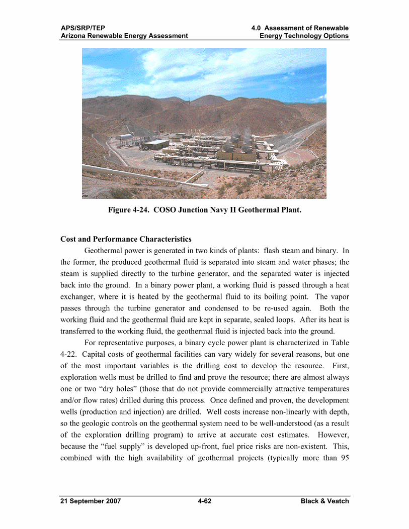
APS/SRP/TEPArizona Renewable Energy Assessment
4.0 Assessment of RenewableEnergy Technology Options
21 September 2007 4-62 Black & Veatch
Figure 4-24. COSO Junction Navy II Geothermal Plant.
Cost and Performance Characteristics Geothermal power is generated in two kinds of plants: flash steam and binary. In
the former, the produced geothermal fluid is separated into steam and water phases; the steam is supplied directly to the turbine generator, and the separated water is injected back into the ground. In a binary power plant, a working fluid is passed through a heat exchanger, where it is heated by the geothermal fluid to its boiling point. The vapor passes through the turbine generator and condensed to be re-used again. Both the working fluid and the geothermal fluid are kept in separate, sealed loops. After its heat is transferred to the working fluid, the geothermal fluid is injected back into the ground.
For representative purposes, a binary cycle power plant is characterized in Table 4-22. Capital costs of geothermal facilities can vary widely for several reasons, but one of the most important variables is the drilling cost to develop the resource. First, exploration wells must be drilled to find and prove the resource; there are almost always one or two “dry holes” (those that do not provide commercially attractive temperatures and/or flow rates) drilled during this process. Once defined and proven, the development wells (production and injection) are drilled. Well costs increase non-linearly with depth, so the geologic controls on the geothermal system need to be well-understood (as a result of the exploration drilling program) to arrive at accurate cost estimates. However, because the “fuel supply” is developed up-front, fuel price risks are non-existent. This, combined with the high availability of geothermal projects (typically more than 95
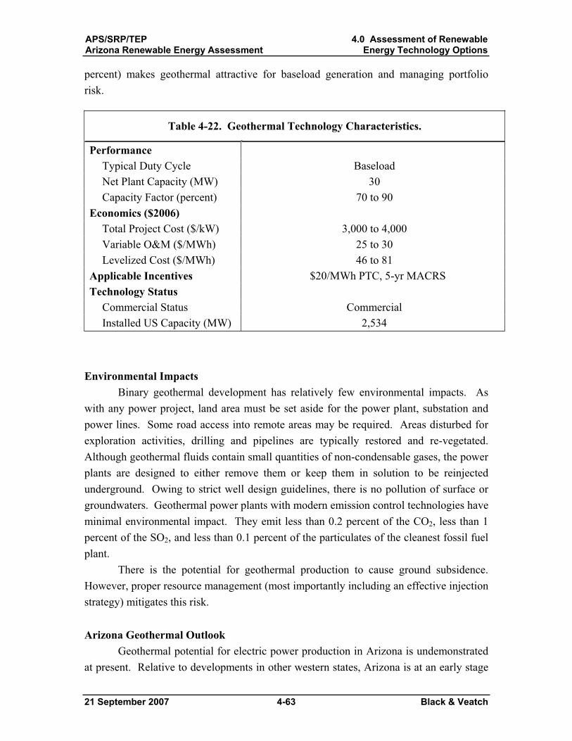
APS/SRP/TEPArizona Renewable Energy Assessment
4.0 Assessment of RenewableEnergy Technology Options
21 September 2007 4-63 Black & Veatch
percent) makes geothermal attractive for baseload generation and managing portfolio risk.
Table 4-22. Geothermal Technology Characteristics.
PerformanceTypical Duty Cycle Baseload Net Plant Capacity (MW) 30 Capacity Factor (percent) 70 to 90
Economics ($2006) Total Project Cost ($/kW) 3,000 to 4,000 Variable O&M ($/MWh) 25 to 30 Levelized Cost ($/MWh) 46 to 81
Applicable Incentives $20/MWh PTC, 5-yr MACRS Technology Status
Commercial Status Commercial Installed US Capacity (MW) 2,534
Environmental Impacts Binary geothermal development has relatively few environmental impacts. As
with any power project, land area must be set aside for the power plant, substation and power lines. Some road access into remote areas may be required. Areas disturbed for exploration activities, drilling and pipelines are typically restored and re-vegetated. Although geothermal fluids contain small quantities of non-condensable gases, the power plants are designed to either remove them or keep them in solution to be reinjected underground. Owing to strict well design guidelines, there is no pollution of surface or groundwaters. Geothermal power plants with modern emission control technologies have minimal environmental impact. They emit less than 0.2 percent of the CO2, less than 1 percent of the SO2, and less than 0.1 percent of the particulates of the cleanest fossil fuel plant.
There is the potential for geothermal production to cause ground subsidence. However, proper resource management (most importantly including an effective injection strategy) mitigates this risk.
Arizona Geothermal Outlook Geothermal potential for electric power production in Arizona is undemonstrated
at present. Relative to developments in other western states, Arizona is at an early stage

APS/SRP/TEPArizona Renewable Energy Assessment
4.0 Assessment of RenewableEnergy Technology Options
21 September 2007 4-64 Black & Veatch
of development. After a long period of relative inactivity, geothermal development in the US is booming. Table 4-23 lists current development prospects as identified by the Geothermal Energy Association. There is one project in Arizona identified with 2 to 20 MW of potential. This is the Clifton project that has been under development by Vulcan, although there is not project activity at this time.
Table 4-23. Current Geothermal Development Prospects.
Projects MW Alaska 2 20.6 Arizona 1 2-20 California 15 821-870 Hawaii 2 38 Idaho 2 36 New Mexico 2 21 Nevada 19 547-661 Oregon 6 186-211 Utah 2 47.6 Total 51 1,720-1,925 Source: Geothermal Energy Association, Jan 2007, http://www.geo-energy.org/
4.8 Fuel Cells Using Renewable Fuels Fuel cell technology has been developed by government agencies and private
corporations. Fuel cells are an important part of space exploration and are receiving considerable attention as an alternative power source for automobiles. In addition to these two applications, fuel cells continue to be considered for power generation for permanent power and intermittent power demands. Figure 4-25 shows an example of a fuel cell in operation.
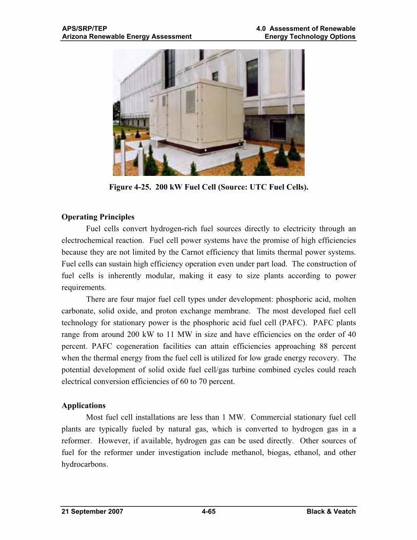
APS/SRP/TEPArizona Renewable Energy Assessment
4.0 Assessment of RenewableEnergy Technology Options
21 September 2007 4-65 Black & Veatch
Figure 4-25. 200 kW Fuel Cell (Source: UTC Fuel Cells).
Operating Principles Fuel cells convert hydrogen-rich fuel sources directly to electricity through an
electrochemical reaction. Fuel cell power systems have the promise of high efficiencies because they are not limited by the Carnot efficiency that limits thermal power systems. Fuel cells can sustain high efficiency operation even under part load. The construction of fuel cells is inherently modular, making it easy to size plants according to power requirements.
There are four major fuel cell types under development: phosphoric acid, molten carbonate, solid oxide, and proton exchange membrane. The most developed fuel cell technology for stationary power is the phosphoric acid fuel cell (PAFC). PAFC plants range from around 200 kW to 11 MW in size and have efficiencies on the order of 40 percent. PAFC cogeneration facilities can attain efficiencies approaching 88 percent when the thermal energy from the fuel cell is utilized for low grade energy recovery. The potential development of solid oxide fuel cell/gas turbine combined cycles could reach electrical conversion efficiencies of 60 to 70 percent.
Applications Most fuel cell installations are less than 1 MW. Commercial stationary fuel cell
plants are typically fueled by natural gas, which is converted to hydrogen gas in a reformer. However, if available, hydrogen gas can be used directly. Other sources of fuel for the reformer under investigation include methanol, biogas, ethanol, and other hydrocarbons.
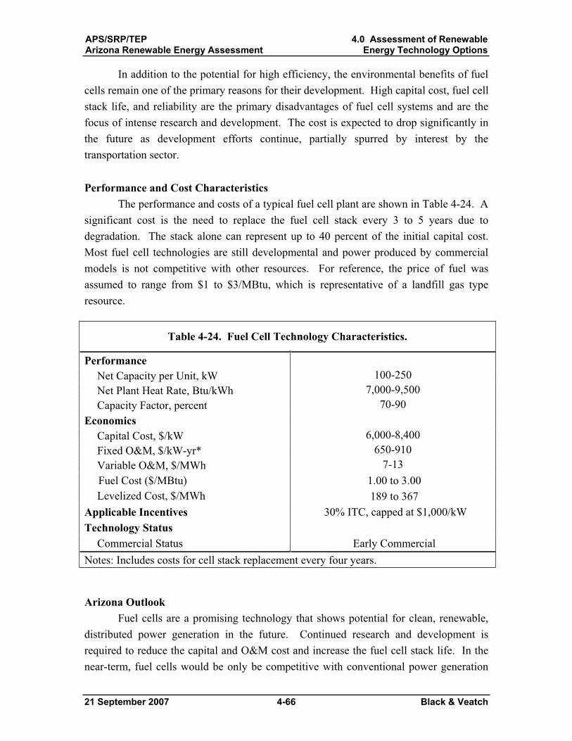
APS/SRP/TEPArizona Renewable Energy Assessment
4.0 Assessment of RenewableEnergy Technology Options
21 September 2007 4-66 Black & Veatch
In addition to the potential for high efficiency, the environmental benefits of fuel cells remain one of the primary reasons for their development. High capital cost, fuel cell stack life, and reliability are the primary disadvantages of fuel cell systems and are the focus of intense research and development. The cost is expected to drop significantly in the future as development efforts continue, partially spurred by interest by the transportation sector.
Performance and Cost Characteristics The performance and costs of a typical fuel cell plant are shown in Table 4-24. A
significant cost is the need to replace the fuel cell stack every 3 to 5 years due to degradation. The stack alone can represent up to 40 percent of the initial capital cost. Most fuel cell technologies are still developmental and power produced by commercial models is not competitive with other resources. For reference, the price of fuel was assumed to range from $1 to $3/MBtu, which is representative of a landfill gas type resource.
Table 4-24. Fuel Cell Technology Characteristics.
PerformanceNet Capacity per Unit, kW 100-250Net Plant Heat Rate, Btu/kWh 7,000-9,500Capacity Factor, percent 70-90
EconomicsCapital Cost, $/kW 6,000-8,400Fixed O&M, $/kW-yr* 650-910Variable O&M, $/MWh 7-13Fuel Cost ($/MBtu) 1.00 to 3.00 Levelized Cost, $/MWh 189 to 367
Applicable Incentives 30% ITC, capped at $1,000/kW Technology Status
Commercial Status Early Commercial Notes: Includes costs for cell stack replacement every four years.
Arizona Outlook Fuel cells are a promising technology that shows potential for clean, renewable,
distributed power generation in the future. Continued research and development is required to reduce the capital and O&M cost and increase the fuel cell stack life. In the near-term, fuel cells would be only be competitive with conventional power generation
APS/SRP/TEPArizona Renewable Energy Assessment
4.0 Assessment of RenewableEnergy Technology Options
21 September 2007 4-67 Black & Veatch
technologies with considerable subsidies, and a low cost (or free) hydrogen fuel source. In the long-term (10-20 years), fuel cells could be a competitive power generation technology, pending advancements in R&D.
Methane sources (such as landfill, manure, MSW) are a good source of renewable hydrogen. Especially at a facility that already harvests the methane for power, reforming the gas instead to produce H2 is a good possibility. Because landfill, and digester gas is low heating value gas, the treatment to make H2 is more attractive. However, currently reciprocating engines are much more economical for these types of fuels.
Arizona State University has a significant fuel cell research effort. Most recently it has garnered some recognition for its work on fuel cells for laptop computer sized equipment. The Salt River Project has had two 5 kW fuel cells (Plug Power and GenSys 5CS) connected to its grid since 2005 for the purposes of testing them in the Arizona heat.
4.9 Compressed Air Energy Storage Although it is not a renewable energy technology, compressed air energy storage
can potentially help enable development of intermittent renewable energy sources, such as wind and solar. The technology is briefly introduced here.
Compressed air energy storage (CAES) is a technique used to supply electrical power to meet peak loads within an electric utility system. This method uses the power surplus from power plants during off-peak periods to compress and store air in an underground formation. The compressed air is later heated (with a fuel) and expanded through a gas turbine expander to produce electrical power during peak demand. A simple compressed air storage plant consists of an air compressor, turbine, generator unit, and a storage vessel. Exhaust gas heat recuperation can be added to increase efficiency.
The thermodynamic cycle for a compressed air storage facility is similar to that of a simple cycle gas turbine. Typically, gas turbines will consume 50 to 60 percent of their net power output to operate an air compressor. In a compressed air storage plant, the air compressor and the turbine are not connected, and the total power generated from the gas turbine is supplied to the electrical grid. By using off-peak energy to compress the air, the need for expensive natural gas or fuel oil is reduced by as much as two thirds, compared with conventional gas turbines.9 This results in a very attractive heat rate for CAES plants, ranging from 4,000 to 5,000 Btu/kWh. Since fuel (typically natural gas) is supplied to the system during the energy generation mode, CAES plants actually provide
9 Nakhamkin, M., Anderson, L., Swenson, E., “AEC 110 MW CAES Plant: Status of Project,” Journal of Engineering for Gas Turbines and Power, October 1992, Vol. 114.
APS/SRP/TEPArizona Renewable Energy Assessment
4.0 Assessment of RenewableEnergy Technology Options
21 September 2007 4-68 Black & Veatch
more electrical power to the grid than was used to compress the air. The capital costs for CAES facilities are approximately the same as a similar sized combined cycle facility.
The location of a CAES plant must be suitable for cavern construction or for the reuse of an existing cavern. However, suitable geology is widespread throughout the United States, with more than 75 percent of the land area containing appropriate geological formations.10 There are three types of formations that can be used to store compressed gases: solution mined reservoirs in salt, conventionally mined reservoirs in salt or hard rock, and naturally occurring porous media reservoirs (aquifers).
CAES can potentially be a good match with renewable energy sources. CAES units are highly flexible; they have quick start-up times, high ramp rates, and good part-load efficiency. These attributes make them suitable to help balance intermittent wind and solar resources. In addition, it is possible that the fuel input needed during the expansion phase of the CAES cycle could be provided by biomass or biofuels.
The basic components of a CAES plant are proven technologies, and CAES units have a reputation for achieving good availability. The first commercial-scale CAES plant in the world was a 290 MW plant in Huntorf, Germany. This plant has been operating since 1978, providing 2 hours of generation with 8 hours of charging. In 1991, a 110 MW CAES facility was installed in McIntosh, Alabama. This plant remains the only US CAES installation, although several new plants have been announced. For example, the Iowa Association of Municipal Utilities is developing the Iowa Stored Energy Park. This project will combine up to about 200 MW of CAES with a wind farm.
Because it operates on the difference between off and on peak electricity prices, the economics of a CAES plant must be evaluated within the context of a specific market. Such an evaluation is outside the scope of this study. However, based on other studies Black & Veatch has performed, the following general conclusions can be drawn:
CAES can be a very competitive option to serve intermediate loads. Because of its low heat rate, CAES can be more economical than combined cycle, especially at higher gas prices. To be cost effective, CAES requires access to low cost, off-peak energy from either coal, nuclear, hydroelectric, or wind facilities. Although CAES can help balance renewable energy resources, there is typically not enough value to justify a CAES project solely for this purpose.If new balancing or back-up capacity must be developed to “firm” wind and solar, simple cycle combustion turbines may offer a less expensive option. CAES can provide high value ancillary services (quick-start, spinning reserve, etc.) that need to be considered in an evaluation of CAES economics.
APS/SRP/TEPArizona Renewable Energy Assessment
4.0 Assessment of RenewableEnergy Technology Options
21 September 2007 4-69 Black & Veatch
The economics of CAES are not straightforward and are not easy to assess without detailed production cost modeling.
Although CAES seems to be gaining increased interest, it is not clear that there is a need for CAES in the near-term in Arizona to enable development of additional renewable resources. Based on the projections in this study, intermittent wind projects (which would benefit most from CAES) will likely comprise a relatively small fraction (< 5 percent) of the overall Arizona energy portfolio going forward. This level of wind penetration should be able to be accommodated without the need for a dedicated CAES facility. For this reason, CAES is not considered further in this study.
4.10 Renewable Energy Technology Summary The technology cost and performance assumptions developed in the previous
sections are summarized in Table 4-25. The values shown in the table were chosen as representative of the technology application in Arizona.
10 Mehta, B., “Compressed Air Energy Storage: CAES Geology,” EPRI Journal, October/November 1992.

APS
/SR
P/TE
PA
rizon
a R
enew
able
Ene
rgy
Ass
essm
ent
4.0
Ass
essm
ent o
f Ren
ewab
le E
nerg
y Te
chno
logy
Opt
ions
21 S
epte
mbe
r 200
7 4-
70
Bla
ck &
Vea
tch
Tab
le4-
25.
Ren
ewab
le T
echn
olog
ies P
erfo
rman
ce a
nd C
ost S
umm
ary.
a
Net
Pla
nt
Cap
acity
,M
W
Net
Pla
nt
Hea
t Rat
e,
Btu
/kW
h
Cap
acity
Fact
orC
apita
l Cos
t, $/
kWFi
xed
O&
M,
$/kW
-yr
Var
iabl
eO
&M
,$/
MW
h
Fuel
Cos
t, $/
MB
tu
Lev
eliz
ed
Cos
t,$/
MW
hD
irect
Bio
mas
s (U
WW
) 35
13
500
70-9
0 27
50-3
500
83
11
1 66
-94
Dire
ct B
iom
ass (
FR)
35
1350
0 70
-90
2750
-350
0 83
11
3
90-1
18
Bio
mas
s IG
CC
(UW
W)
35
1000
0-11
500
70-9
0 30
00-4
000
83
11
1 65
-99
Bio
mas
s IG
CC
(FR
) 35
10
000-
1150
0 70
-90
3000
-400
0 83
11
3
82-1
20
Cof
ired
Bio
. (UW
W)
30
1000
0 70
-90
300-
500
5-15
0
-0.5
c0-
9C
ofire
d B
io. (
FR)
30
1000
0 70
-90
300-
500
5-15
0
1 18
-27
Ana
erob
ic D
iges
tion
0.15
11
500
70-9
0 40
00-6
000
0 17
0
68-1
26
Land
fill G
as
2-10
11
500
70-9
0 15
00-2
000
0 17
1-
3 40
-80
Sola
r The
rmal
(tro
ugh)
10
0
37-4
3 54
00-6
300
0 20
-25
13
2-17
6 So
lar T
herm
al (d
ish)
14
20-2
5 50
00-6
000
0 10
-20
18
4-28
1 So
lar P
V (r
esid
entia
l) 0.
004
18
85
00-1
2500
50
0
35
8-50
9 So
lar P
V (c
omm
erci
al)
0.25
0
20
7000
-900
0 30
0
32
1-40
7 So
lar P
V (u
tility
) 3
22
60
00-8
000
30
0
278-
365
Hyd
ro (n
ew)
<50
40
-60
2500
-400
0 5-
25
5-6
44
-121
H
ydro
(inc
rem
enta
l) 1-
160
40
-60
600-
3000
5-
25
4-6
5-
92
Win
d 50
-100
25-3
5 16
00-1
900
28
8
51-9
3 G
eoth
erm
al
30
70
-90
3000
-400
0 0
25-3
0
46-8
1 Fu
el C
ells
0.
1-.2
5 70
00-9
500
70-9
0 50
00-7
400
650-
910
7-13
1-
3 18
9-36
7 N
otes
:a
Incl
udes
app
licab
le in
cent
ives
, sub
sidi
es, e
tc.
All
cost
s are
in 2
007
dolla
rs.
b
UW
W =
Urb
an W
ood
Was
te ;
FR =
For
estry
Res
idue
s c
Ass
umes
pay
men
t for
dis
posa
l of w
aste
not
take
n to
land
fill.
APS/SRP/TEPArizona Renewable Energy Assessment
4.0 Assessment of RenewableEnergy Technology Options
21 September 2007 4-71 Black & Veatch
4.10.1 Relative Costs Of the renewable energy technologies evaluated, cofiring has the lowest capital
cost per kW installed at $300-500/kW. The majority of the capital costs are associated with adding material handling equipment to an existing coal plant, as opposed to development of new plants for most other technologies. Wind has the next lowest capital cost at $1,600-1,900/kW. This has been a main driver in the 30 percent annual increase in wind installations worldwide over the last five years. Recently, however, system costs have begun to rise. In comparison, conventional biomass and geothermal technologies have capital costs in the range of $2,750-3,500/kW and $3,000-4,000/kW, respectively. The high cost of biomass plants is due to their relatively small size, extensive fuel and ash handling requirements, and the need for a robust plant design to handle the variability in the fuel quality. New hydroelectric power plants have a wide range of capital costs from $2,500-4,000/kW. Given that hydroelectric technology is quite mature and costs are low, the civil work that needs to be done to build dams and penstocks tends to be the driving factor behind the capital cost of these systems. Incremental hydroelectric improvements can be much lower in costs. Photovoltaic systems are by far the most expensive renewable energy technology, with capital costs from $6,000-12,500/kW and a capacity factor of only about 20 percent.
When comparing the levelized cost of energy produced by these systems, biomass, hydroelectric, anaerobic digestion, landfill gas, hydroelectric, wind and geothermal all have the potential to produce power at rates competitive with new coal and gas power generation. Although these resources have high capital costs, low operating costs combined with high operating capacity factors reduce the overall life-cycle costs.
Continued improvements will result in improvements in efficiency, capital cost, and operating and maintenance cost for several of the technologies. The technology areas where the levelized cost of power production should come down in the future are wind, biomass gasification, photovoltaics, solar thermal, and fuel cells. Large improvements are expected for solar technologies, with relatively modest improvements in other technologies.
4.10.2 Recommendations for Further Study Based on the profiles described previously in this study, Table 4-26 presents our
recommendations for further study. Due to their resource potential or low cost, these are the most promising technologies in Arizona.
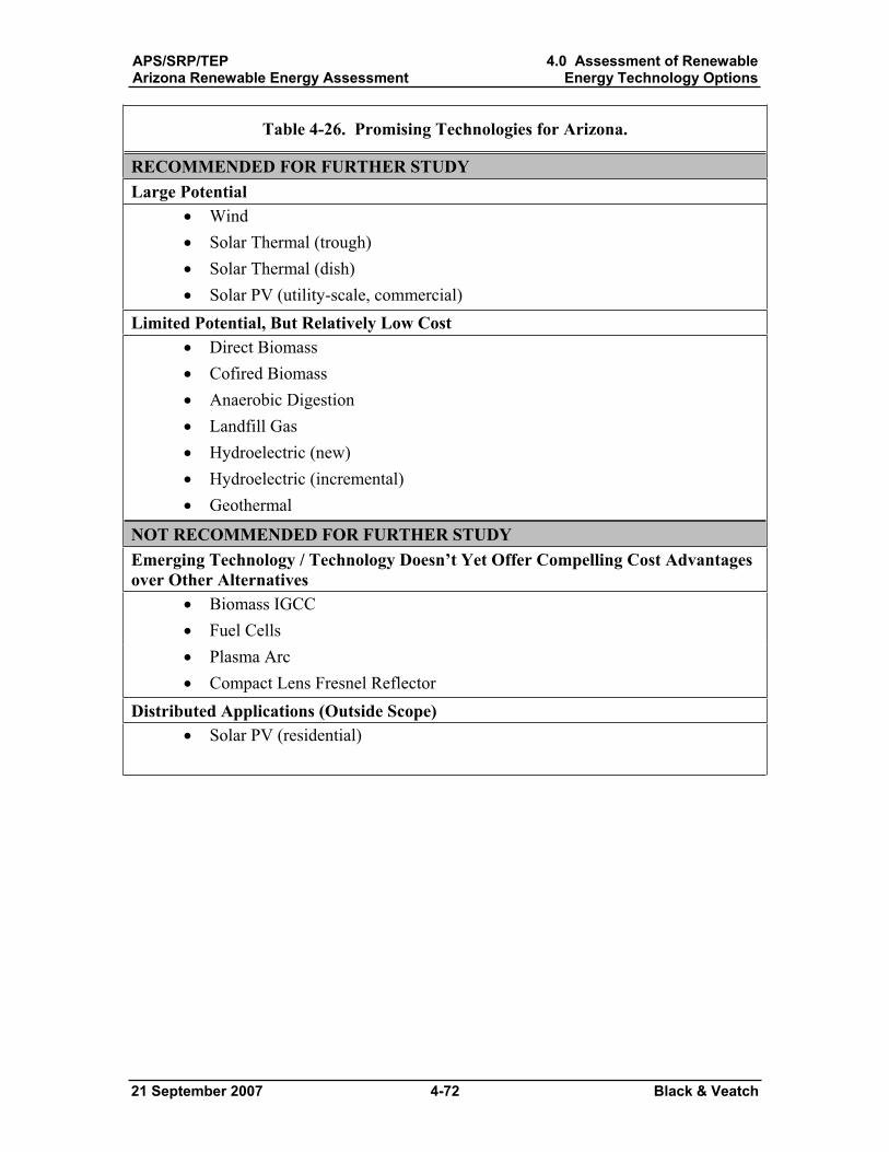
APS/SRP/TEPArizona Renewable Energy Assessment
4.0 Assessment of RenewableEnergy Technology Options
21 September 2007 4-72 Black & Veatch
Table 4-26. Promising Technologies for Arizona.
RECOMMENDED FOR FURTHER STUDY Large Potential
Wind Solar Thermal (trough) Solar Thermal (dish) Solar PV (utility-scale, commercial)
Limited Potential, But Relatively Low Cost Direct Biomass Cofired Biomass Anaerobic Digestion Landfill Gas Hydroelectric (new) Hydroelectric (incremental) Geothermal
NOT RECOMMENDED FOR FURTHER STUDY Emerging Technology / Technology Doesn’t Yet Offer Compelling Cost Advantages over Other Alternatives
Biomass IGCC Fuel Cells Plasma Arc Compact Lens Fresnel Reflector
Distributed Applications (Outside Scope) Solar PV (residential)
APS/SRP/TEPArizona Renewable Energy Assessment
5.0 Renewable ResourceAssessment
21 September 2007 5-1 Black & Veatch
5.0 Renewable Resource Assessment
The objective of this section is to assess the renewable energy resources of Arizona that are suitable for development in the near- to mid-term (next 20 years). Potential development prospects are identified, levelized generation costs are calculated, and a set of supply curves is developed. An end result of this process was the identification of a list of over 100 hypothetical renewable energy projects that might be developed to meet demands for renewable energy in Arizona.
The technologies reviewed in this section are: Direct Fired and Cofired Biomass Landfill Gas Anaerobic Digestion Solar Thermal Electric Solar Photovoltaic HydroelectricWind Power Geothermal
All costs presented in this section are in 2007$ unless otherwise stated. Additional economic assumptions impacting the projects are presented in Section 7.2.
5.1 Direct Fired and Cofired Biomass Both direct-fired biomass and cofired biomass were identified as promising
technologies in the first stage of the analysis. Cofiring is generally more economical, but it is limited to locations where biomass is available near an existing coal plant. If there are no coal plants in the vicinity, direct fired biomass is a more appropriate technology. This section characterizes the resources suitable for both technologies.
5.1.1 General Methodology The feasibility of direct fired and cofired biomass projects is largely dependent
upon obtaining an economical biomass fuel supply. A high-level review of biomass resources based primarily on data assembled by the National Renewable Energy Laboratory (NREL) was presented in Section 4 This estimate provided county-level estimates of biomass resources with the state. As discussed in Section 4, the national forests in Coconino, Navajo and Apache counties provide the largest sources of woody biomass resources. There are significant quantities of residues from forest thinning activities, and these residues are supplemented by mill residues from the Fort Apache
APS/SRP/TEPArizona Renewable Energy Assessment
5.0 Renewable ResourceAssessment
21 September 2007 5-2 Black & Veatch
Timber Company (FATCO). Significant quantities of urban wood waste are found in the Phoenix and Tucson area. These metropolitan areas are surrounded by agricultural areas, which provide crop residues for smaller scale biomass energy facilities.
To obtain information regarding specific point sources of biomass resources that could be utilized to secure biomass fuel for actual biomass projects, Black & Veatch contacted potential suppliers of biomass resources via telephone. An initial round of phone calls were made to potential suppliers of biomass identified in a previous assessment of Arizona’s biomass resources. This previous assessment, conducted by Black & Veatch in 2005 as part of a larger study for APS, identified over 60 potential suppliers, and the objective of the phone survey conducted for this present study was to verify that the resource previously identified were currently available and to determine if any additional resources were available. The focus of this effort was in the northern and eastern portions of the state as this is where much of the state’s wood resources are located.
Following the initial round of calls, additional suppliers and agencies were contacted. Forestry and renewable energy experts at the University of Arizona and Northern Arizona University were consulted regarding biomass resources within the state, and national and state forestry officials were contacted to obtain information regarding potential forest thinning residues. Landfills were contacted to determine the availability of urban wood waste streams for use in biomass energy facilities.
Based on the conversations with biomass suppliers, forestry officials, and renewable energy experts, key findings of the updated assessment include:
In general, the survey confirmed the presence of the biomass resources previously identified. One significant source of mill residues not previously identified was found. Southwest Forest Products has constructed a new sawmill in Ash Fork, which generates roughly 55 dry tons per day (dtpd) of mill residues. A significant competitor of biomass resources was also identified. An oriented strand board manufacturing facility is being developed in Winslow. This proposed facility would consume 1 million tons per year of biomass and may begin operation as soon as winter of 2008. The significant suppliers of primary mill residues are summarized in Table 5-1.The United States Forestry Service provided the current forest treatment plan for the national forests in Arizona. The estimated residues from forest thinning activities are summarized in Table 5-2.
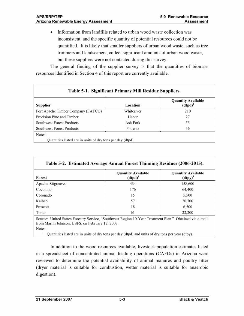
APS/SRP/TEPArizona Renewable Energy Assessment
5.0 Renewable ResourceAssessment
21 September 2007 5-3 Black & Veatch
Information from landfills related to urban wood waste collection was inconsistent, and the specific quantity of potential resources could not be quantified. It is likely that smaller suppliers of urban wood waste, such as tree trimmers and landscapers, collect significant amounts of urban wood waste, but these suppliers were not contacted during this survey.
The general finding of the supplier survey is that the quantities of biomass resources identified in Section 4 of this report are currently available.
Table 5-1. Significant Primary Mill Residue Suppliers.
Supplier Location Quantity Available
(dtpd)1
Fort Apache Timber Company (FATCO) Whiteriver 210 Precision Pine and Timber Heber 27 Southwest Forest Products Ash Fork 55 Southwest Forest Products Phoenix 36 Notes:
1 Quantities listed are in units of dry tons per day (dtpd).
Table 5-2. Estimated Average Annual Forest Thinning Residues (2006-2015).
Forest Quantity Available
(dtpd)1Quantity Available
(dtpy)1
Apache-Sitgreaves 434 158,600 Coconino 176 64,400 Coronado 15 5,500 Kaibab 57 20,700 Prescott 18 6,500 Tonto 61 22,200 Source: United States Forestry Service, “Southwest Region 10-Year Treatment Plan.” Obtained via e-mail from Marlin Johnson, USFS, on February 12, 2007. Notes:
1 Quantities listed are in units of dry tons per day (dtpd) and units of dry tons per year (dtpy).
In addition to the wood resources available, livestock population estimates listed in a spreadsheet of concentrated animal feeding operations (CAFOs) in Arizona were reviewed to determine the potential availability of animal manures and poultry litter (dryer material is suitable for combustion, wetter material is suitable for anaerobic digestion).
APS/SRP/TEPArizona Renewable Energy Assessment
5.0 Renewable ResourceAssessment
21 September 2007 5-4 Black & Veatch
Following the rounds of resource assessment and review, the biomass resource estimates were aggregated. Considering the geographic distribution of the resources and the quantities available, two potential cofiring projects and one potential direct fired project were identified. The estimate of available resources is considered to be somewhat conservative, and it is likely that additional biomass projects could be developed if all of the resources identified were utilized by biomass facilities. However, biomass project developers generally attempt to identify at least 2 to 3 times the required tonnage needed for full-scale operation, and this assumption was used as a limit for the projects proposed in this study. Furthermore, the potential for biomass energy in Arizona is limited due to competition for the existing resources. In addition to typical competition for wood residues such as animal bedding and the new oriented strand board facility being developed in Winslow, there are also at least two significant biomass consumers in eastern Arizona:
Forest Energy Corporation: Located in Show Low, Forest Energy produces almost 200 dry tons per day of pelletized wood, which is used as fuel for residential and commercial heating. Pellet fuel is generally thought to be too expensive for utility applications.Snowflake White Mountain Power (SWMP): Located near Snowflake, SWMP is a 24 MW biomass power facility scheduled to begin operation in 2008. In addition to burning recycled paper fibers from Abitibi, this facility will require roughly 250 additional dry tons per day of biomass.
The competition from these operations and other potential consumers of biomass resources will constrain the capacities of other biomass facilities.
5.1.2 Major Assumptions The two potential cofiring projects identified in Arizona are assumed to be located
at TEP’s Springerville Generating Station and APS’s Cholla Generating Station. Cofiring could also take place at SRP’s Coronado station (with similar economics to that shown for Springerville). However, there may not be enough resources to support three cofiring projects in eastern Arizona.
The following assumptions were made in the evaluation of cofired biomass potential.
The cofiring projects would employ a gasification system close coupled to the existing boiler. A Net Plant Heat Rate (NPHR) of 11,000 Btu/kWh was assumed for Cholla, based on boiler modeling conducted by Black & Veatch in a previous study. An NPHR of 10,000 was assumed for Springerville, based on information
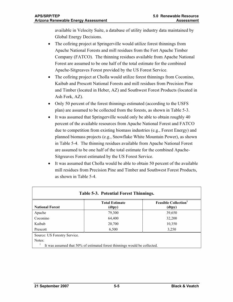
APS/SRP/TEPArizona Renewable Energy Assessment
5.0 Renewable ResourceAssessment
21 September 2007 5-5 Black & Veatch
available in Velocity Suite, a database of utility industry data maintained by Global Energy Decisions.The cofiring project at Springerville would utilize forest thinnings from Apache National Forests and mill residues from the Fort Apache Timber Company (FATCO). The thinning residues available from Apache National Forest are assumed to be one half of the total estimate for the combined Apache-Sitgreaves Forest provided by the US Forest Service. The cofiring project at Cholla would utilize forest thinnings from Coconino, Kaibab and Prescott National Forests and mill residues from Precision Pine and Timber (located in Heber, AZ) and Southwest Forest Products (located in Ash Fork, AZ). Only 50 percent of the forest thinnings estimated (according to the USFS plan) are assumed to be collected from the forests, as shown in Table 5-3.It was assumed that Springerville would only be able to obtain roughly 40 percent of the available resources from Apache National Forest and FATCO due to competition from existing biomass industries (e.g., Forest Energy) and planned biomass projects (e.g., Snowflake White Mountain Power), as shown in Table 5-4. The thinning residues available from Apache National Forest are assumed to be one half of the total estimate for the combined Apache-Sitgreaves Forest estimated by the US Forest Service. It was assumed that Cholla would be able to obtain 50 percent of the available mill residues from Precision Pine and Timber and Southwest Forest Products, as shown in Table 5-4.
Table 5-3. Potential Forest Thinnings.
National Forest Total Estimate
(dtpy) Feasible Collection1
(dtpy) Apache 79,300 39,650 Coconino 64,400 32,200 Kaibab 20,700 10,350 Prescott 6,500 3,250 Source: US Forestry Service. Notes:
1 It was assumed that 50% of estimated forest thinnings would be collected.
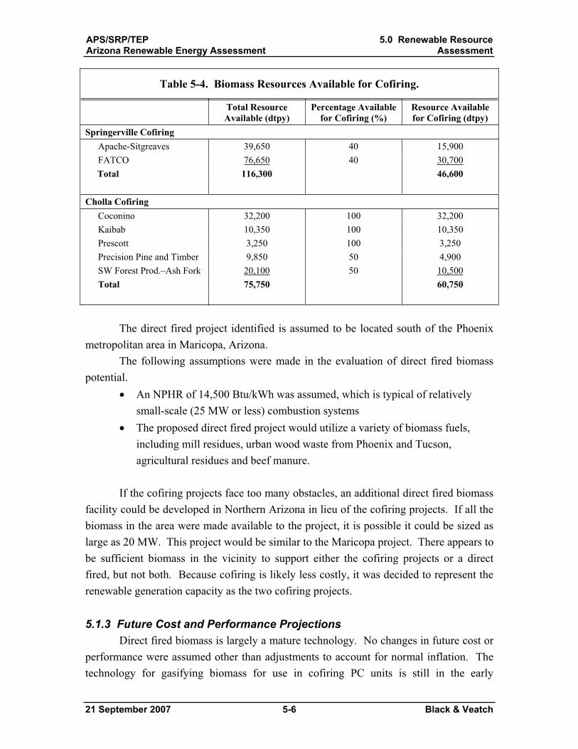
APS/SRP/TEPArizona Renewable Energy Assessment
5.0 Renewable ResourceAssessment
21 September 2007 5-6 Black & Veatch
Table 5-4. Biomass Resources Available for Cofiring.
Total Resource Available (dtpy)
Percentage Available for Cofiring (%)
Resource Available for Cofiring (dtpy)
Springerville Cofiring Apache-Sitgreaves 39,650 40 15,900 FATCO 76,650 40 30,700 Total 116,300 46,600 Cholla Cofiring Coconino 32,200 100 32,200 Kaibab 10,350 100 10,350 Prescott 3,250 100 3,250 Precision Pine and Timber 9,850 50 4,900 SW Forest Prod.–Ash Fork 20,100 50 10,500 Total 75,750 60,750
The direct fired project identified is assumed to be located south of the Phoenix metropolitan area in Maricopa, Arizona.
The following assumptions were made in the evaluation of direct fired biomass potential.
An NPHR of 14,500 Btu/kWh was assumed, which is typical of relatively small-scale (25 MW or less) combustion systems The proposed direct fired project would utilize a variety of biomass fuels, including mill residues, urban wood waste from Phoenix and Tucson, agricultural residues and beef manure.
If the cofiring projects face too many obstacles, an additional direct fired biomass facility could be developed in Northern Arizona in lieu of the cofiring projects. If all the biomass in the area were made available to the project, it is possible it could be sized as large as 20 MW. This project would be similar to the Maricopa project. There appears to be sufficient biomass in the vicinity to support either the cofiring projects or a direct fired, but not both. Because cofiring is likely less costly, it was decided to represent the renewable generation capacity as the two cofiring projects.
5.1.3 Future Cost and Performance Projections Direct fired biomass is largely a mature technology. No changes in future cost or
performance were assumed other than adjustments to account for normal inflation. The technology for gasifying biomass for use in cofiring PC units is still in the early
APS/SRP/TEPArizona Renewable Energy Assessment
5.0 Renewable ResourceAssessment
21 September 2007 5-7 Black & Veatch
commercialization phase. While cost and performance improvements of such systems may change as expertise grows, improvements are expected to be relatively small. Therefore, no changes in future cost or performance were assumed other than adjustments to account for normal inflation.
5.1.4 Data Sources Data sources used in this analysis included:
Black & Veatch, “Cholla #1 Biomass Cofiring Conceptual Design Study.”December, 2005. Spreadsheet of Concentrated Animal Feeding Operations (CAFO) in Arizona, provided by Thomas Ramey of APS on November 30, 2006. United States Forestry Service, “Southwest Region 10-Year Treatment Plan.” Obtained via e-mail from Marlin Johnson, USFS, on February 12, 2007. Survey of Arizona biomass suppliers, forestry officials and landfills conducted by telephone. Survey conducted January-March, 2007.
5.1.5 Projects Identified As mentioned above, two biomass cofiring projects have been identified. Based
on the resources available and the assumptions listed above, a 10 MW cofiring project is feasible at Springerville Generating Station, and a 10 MW cofiring project is feasible at Cholla Generating Station. Assuming a capacity factor of 80 percent for both projects, annual biomass generation at Springerville and Cholla would be approximately 70 GWh/yr. These generation amounts do not represent additional generation, rather they represent displacement of coal with a renewable fuel. It is expected permitting and construction of the cofiring projects could be conducted in 18 to 24 months. Given a notice to proceed (NTP) of January 1, 2008, both cofiring projects could be operational by January 1, 2010.
A potential direct fired project has been identified south of the Phoenix metropolitan area. Based on the geographic distribution of the potential biomass resources, a likely potential site for this facility is Maricopa, Arizona. This location would allow the facility to utilize mill residues and urban wood wastes from Phoenix, urban wood wastes from Tucson and agricultural residues from Maricopa and Pinal counties.
A detailed permitting study was not completed for this task. However, both Maricopa County and Pinal County, in which the Maricopa facility would be located, are non-attainment areas for NOx and PM10. It is likely that a Selective Non-Catalytic Reduction (SNCR) would be required to control NOx, and a baghouse or electrostatic
APS/SRP/TEPArizona Renewable Energy Assessment
5.0 Renewable ResourceAssessment
21 September 2007 5-8 Black & Veatch
precipitator (ESP) would be required to control particulate. A small scrubber may be necessary depending on the fuel mix. Although it is a relatively small plant, it is possible that the biomass facility would be considered a major source for these pollutants, in which case the purchase of offsets would also be required. A detailed review of these issues was beyond the scope of this study.
The proposed project has a nominal capacity of 20 MW, and assuming a capacity factor of 80 percent, the facility would produce roughly 140 GWh per year. It is expected permitting and construction of the direct fired project could be conducted in 42 to 48 months. Given a notice to proceed (NTP) of January 1, 2008, the Maricopa direct fired biomass project would likely be operational by January 1, 2012.
Table 5-5 shows the direct fired and cofired biomass projects identified for this study. All characteristics are year 2007 values, before any future cost and performance modifications have been made. Figure 5-1 shows the supply curve for cofired biomass and direct fired biomass projects. For the purposes of visualizing the projects on the supply curve, it has been assumed that all projects could be built in 2007. Appendix A shows a consolidated list of projects; Appendix B shows the same list with forecast levelized costs for each project from 2007 to 2025.
Considering the other renewable energy options evaluated in this study, the costs of the two cofiring projects are relatively low (about $60/MWh in 2010), and the costs of cofiring are certainly lower than the direct fired project (about $162/MWh in 2012). In general, the costs of biomass in Arizona are relatively high due to the lack of low cost biomass and the small scale of biomass projects.
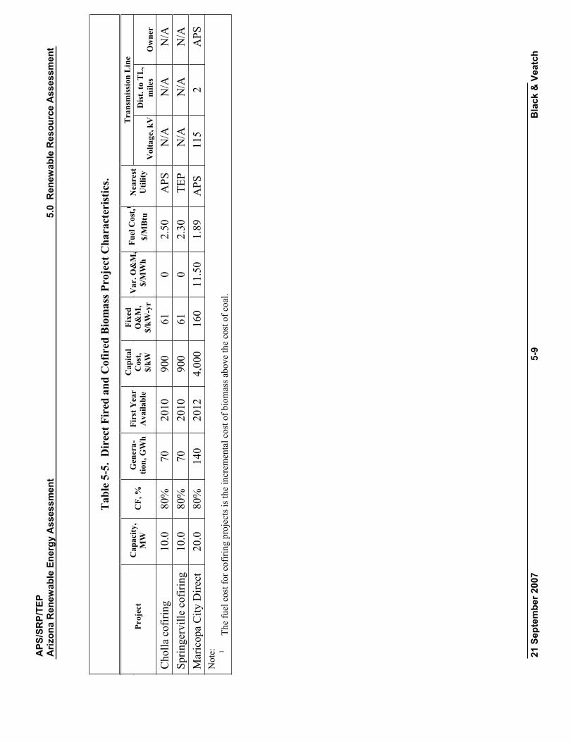
APS
/SR
P/TE
PA
rizon
a R
enew
able
Ene
rgy
Ass
essm
ent
5.0
Ren
ewab
le R
esou
rce
Ass
essm
ent
21 S
epte
mbe
r 200
7 5-
9 B
lack
& V
eatc
h
Tab
le5-
5. D
irec
t Fir
ed a
nd C
ofir
ed B
iom
ass P
roje
ct C
hara
cter
istic
s.
Tra
nsm
issi
on L
ine
Proj
ect
Cap
acity
, M
WC
F, %
G
ener
a-tio
n, G
Wh
Firs
t Yea
r A
vaila
ble
Cap
ital
Cos
t, $/
kW
Fixe
d O
&M
, $/
kW-y
r
Var
. O&
M,
$/M
Wh
Fuel
Cos
t,1
$/M
Btu
Nea
rest
U
tility
V
olta
ge, k
VD
ist.
to T
L,
mile
s O
wne
r
Cho
lla c
ofiri
ng
10.0
80
%
70
2010
90
0 61
0
2.50
A
PS
N/A
N
/A
N/A
Sp
ringe
rvill
e co
firin
g 10
.0
80%
70
20
10
900
61
0 2.
30
TEP
N/A
N
/A
N/A
M
aric
opa
City
Dire
ct
20.0
80
%
140
2012
4,
000
160
11.5
0 1.
89
APS
11
5 2
APS
Not
e:
1Th
e fu
el c
ost f
or c
ofiri
ng p
roje
cts i
s the
incr
emen
tal c
ost o
f bio
mas
s abo
ve th
e co
st o
f coa
l.
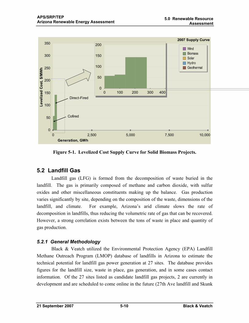
APS/SRP/TEPArizona Renewable Energy Assessment
5.0 Renewable ResourceAssessment
21 September 2007 5-10 Black & Veatch
0 2,500 5,000 7,500 10,0000
50
100
150
200
250
300
350
Generation, GWh
Leve
lized
Cos
t, $/
MW
h
WindBiomass SolarHydroGeothermal
2007 Supply Curve
Direct-Fired
Cofired
0 100 200 300 4000
50
100
150
200
0 100 200 300 4000
50
100
150
200
0 100 200 300 4000
50
100
150
200
0 100 200 300 4000
50
100
150
200
Figure 5-1. Levelized Cost Supply Curve for Solid Biomass Projects.
5.2 Landfill Gas Landfill gas (LFG) is formed from the decomposition of waste buried in the
landfill. The gas is primarily composed of methane and carbon dioxide, with sulfur oxides and other miscellaneous constituents making up the balance. Gas production varies significantly by site, depending on the composition of the waste, dimensions of the landfill, and climate. For example, Arizona’s arid climate slows the rate of decomposition in landfills, thus reducing the volumetric rate of gas that can be recovered. However, a strong correlation exists between the tons of waste in place and quantity of gas production.
5.2.1 General Methodology Black & Veatch utilized the Environmental Protection Agency (EPA) Landfill
Methane Outreach Program (LMOP) database of landfills in Arizona to estimate the technical potential for landfill gas power generation at 27 sites. The database provides figures for the landfill size, waste in place, gas generation, and in some cases contact information. Of the 27 sites listed as candidate landfill gas projects, 2 are currently in development and are scheduled to come online in the future (27th Ave landfill and Skunk
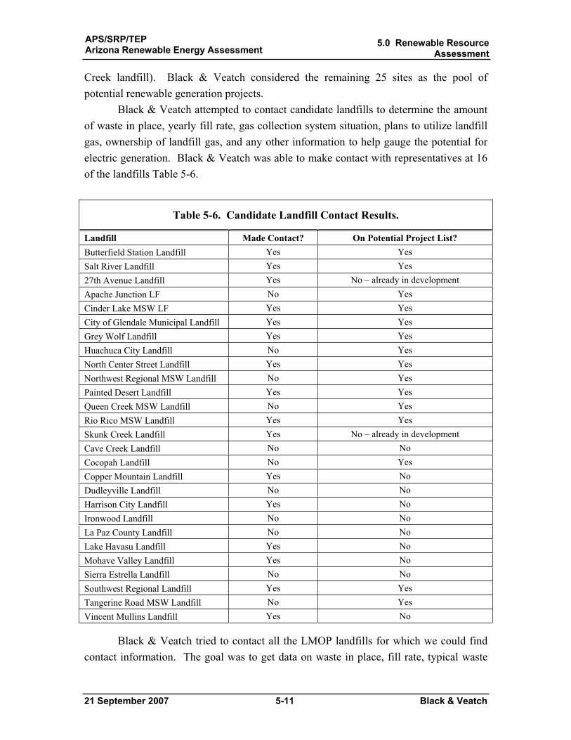
APS/SRP/TEPArizona Renewable Energy Assessment
5.0 Renewable ResourceAssessment
21 September 2007 5-11 Black & Veatch
Creek landfill). Black & Veatch considered the remaining 25 sites as the pool of potential renewable generation projects.
Black & Veatch attempted to contact candidate landfills to determine the amount of waste in place, yearly fill rate, gas collection system situation, plans to utilize landfill gas, ownership of landfill gas, and any other information to help gauge the potential for electric generation. Black & Veatch was able to make contact with representatives at 16 of the landfills Table 5-6.
Table 5-6. Candidate Landfill Contact Results.
Landfill Made Contact? On Potential Project List? Butterfield Station Landfill Yes Yes Salt River Landfill Yes Yes 27th Avenue Landfill Yes No – already in development Apache Junction LF No Yes Cinder Lake MSW LF Yes Yes City of Glendale Municipal Landfill Yes Yes Grey Wolf Landfill Yes Yes Huachuca City Landfill No Yes North Center Street Landfill Yes Yes Northwest Regional MSW Landfill No Yes Painted Desert Landfill Yes Yes Queen Creek MSW Landfill No Yes Rio Rico MSW Landfill Yes Yes Skunk Creek Landfill Yes No – already in development Cave Creek Landfill No No Cocopah Landfill No Yes Copper Mountain Landfill Yes No Dudleyville Landfill No No Harrison City Landfill Yes No Ironwood Landfill No No La Paz County Landfill No No Lake Havasu Landfill Yes No Mohave Valley Landfill Yes No Sierra Estrella Landfill No No Southwest Regional Landfill Yes Yes Tangerine Road MSW Landfill No Yes Vincent Mullins Landfill Yes No
Black & Veatch tried to contact all the LMOP landfills for which we could find contact information. The goal was to get data on waste in place, fill rate, typical waste
APS/SRP/TEPArizona Renewable Energy Assessment
5.0 Renewable ResourceAssessment
21 September 2007 5-12 Black & Veatch
composition, gas production rate, gas collection system status, gas rights ownership, and known plans for using gas for generation. For some landfills it was difficult to reach a manager or engineer who was knowledgeable about the factors needed to assess the landfill’s potential. For all landfills it was also difficult to get sufficient information on all pertinent factors needed to estimate generation potential with a high degree of accuracy. Additional information obtained from the phone survey helped better determine which projects have real potential, approximate how much generation could be expected, and estimate the earliest year each project could come online if project development were prioritized.
Some landfills were removed from the potential project list due to extremely small volumes and limited prospects for achieving a critical mass to make development worthwhile. For promising sites that we were not able to contact, we used the information included in the LMOP database to assess potential.
5.2.2 Major Assumptions The following assumptions were made in the evaluation of landfill gas potential.One million tons of waste in place can support 260 kW of generation capacity. This number was obtained by “normalizing” projections for Arizona landfill gas projects in development to data from previous landfill gas studies, based on waste in place. One million tons of waste in temperate conditions would generate gas sufficient to sustain 700+ kW of generation. While some arid landfills add water and microorganisms to the waste to increase the rate of gas production, all landfills were modeled to have the same waste to generation ratio. It should be noted that Black & Veatch did not prepare gas flow models for any of the potential projects. Although microturbines, larger combustion turbines, and other types of power conversion equipment are used to convert landfill gas to electricity, internal combustion engines account for a great majority of installations. Cost and performance data for internal combustion engines was used as a basis for this study.An annual capacity factor of 80 percent is assumed for all landfill gas projects. Responsibility for the gas collection system cost and maintenance was assumed to be on the landfill owner. Landfills that cannot support electric generation of at least than 250 kW were not included in the list of potential projects.
APS/SRP/TEPArizona Renewable Energy Assessment
5.0 Renewable ResourceAssessment
21 September 2007 5-13 Black & Veatch
Capital cost estimates were based on guidance from the EPA LMOP and range from $2330/kW for a 250 kW facility to $1980/kW for a 5 MW facility. These estimates do not include the cost of installing a gas collection system. Project construction period is one year. Operating and maintenance costs were estimated to be $17.5/MWh for all generation levels. This includes both fixed and variable cost components. Specific transmission lines were not identified. It was assumed that all landfills are currently being served with power, and the generation would back feed. Projects larger than 1 MW are assumed to have a small 34.5 kV substation.Interconnection costs are included in the capital costs for projects less than 1 MW. Landfill gas fuel cost was assumed to be $2/MBtu. This is the cost that a project developer would pay for the rights to the gas. This cost would support maintenance of the landfill gas collection system.
5.2.3 Future Cost and Performance Projections Power generation from landfill gas is a largely a mature technology. No changes
in future cost or performance were assumed other than adjustments to account for inflation.
5.2.4 Data Sources Data sources used in this analysis included:
EPA LMOP database. Available at http://epa.gov/lmop/proj/xls/lmopdata.xlsEPA LOMP program. Available at http://epa.gov/lmop/Survey of Arizona landfills conducted by telephone. Survey conducted January-March, 2007.
5.2.5 Projects Identified Fifteen potential projects were identified, totaling 9.8 MW of capacity and
68 GWh of annual generation, most of which could be available by 2010 if development were prioritized. As mentioned earlier, this capacity is much smaller than what would be expected for similar sized landfills in other states due to Arizona’s dry climate. However, because the refuse in arid landfills decomposes at a slower rate, the gas production is expected to last longer than in temperate landfills.
APS/SRP/TEPArizona Renewable Energy Assessment
5.0 Renewable ResourceAssessment
21 September 2007 5-14 Black & Veatch
The potential Arizona projects modeled in the supply curves do not include two projects that are currently under development—27th Ave. landfill (3 MW of capacity, online in 2008) and Skunk Creek landfill (3 MW of capacity, online in 2009). All of the candidate projects are less than 3 MW in capacity and most are less than 1 MW. Most of the projects are located near transmission lines owned by SRP or APS.
Many of the identified projects are not far-removed from development and commercial operation. Most of the sites already have a gas collection system in place and could have online generation by 2010. As these projects are smaller in scale than other projects such as wind farms or solar trough fields, they are better suited for coming online in the near future to increase Arizona’s developed renewable energy. However, there are not enough landfill gas resources in Arizona to make landfill gas facilities a large portion of the state’s overall renewable energy portfolio. Additionally, the economics for small landfill projects can be challenging. Development costs are prohibitively high for any one project to absorb all of the costs; individually projects are not attractive, but collectively they are acceptable. Black & Veatch would recommend a small-scale modular technology with lower capital and maintenance costs, such as provided by INGENCO. INGENCO provides small-scale engines designed to be modularly installed in landfills that are not viable for other types of equipment. INGENCO projects have potentially lower construction and maintenance costs than the “typical” landfill gas project characteristics assumed for this study.
Table 5-7 shows the landfill gas projects identified for this study. All characteristics are year 2007 values, before any future cost and performance modifications have been made. Figure 5-2 shows the supply curve for landfill gas generation potential (anaerobic digestion projects are also shown). For the purposes of visualizing the projects on the supply curve, it has been assumed that all projects could be built in 2007.
The overall prospects for landfill gas generation are small. Landfill gas projects can take less time to develop than large solar or wind projects, so landfill gas may play a more significant role in the near term.
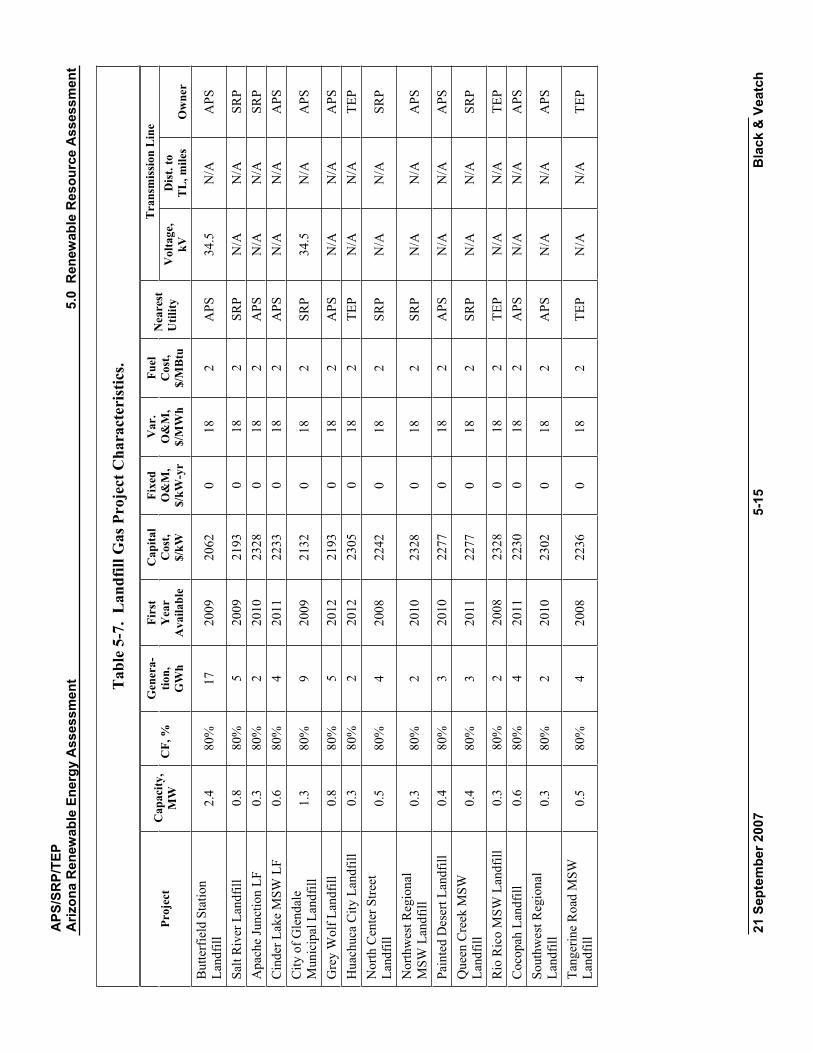
APS
/SR
P/TE
PA
rizon
a R
enew
able
Ene
rgy
Ass
essm
ent
5.0
Ren
ewab
le R
esou
rce
Ass
essm
ent
21 S
epte
mbe
r 200
7 5-
15
Bla
ck &
Vea
tch
Tab
le5-
7. L
andf
ill G
as P
roje
ct C
hara
cter
istic
s.
Tra
nsm
issi
on L
ine
Proj
ect
Cap
acity
, M
WC
F, %
G
ener
a-tio
n,G
Wh
Firs
tY
ear
Ava
ilabl
e
Cap
ital
Cos
t, $/
kW
Fixe
d O
&M
, $/
kW-y
r
Var
. O
&M
, $/
MW
h
Fuel
C
ost,
$/M
Btu
Nea
rest
U
tility
V
olta
ge,
kVD
ist.
to
TL
, mile
s O
wne
r B
utte
rfie
ld S
tatio
n La
ndfil
l 2.
4 80
%
17
2009
20
62
0 18
2
APS
34
.5
N/A
A
PS
Salt
Riv
er L
andf
ill
0.8
80%
5
2009
21
93
0 18
2
SRP
N/A
N
/A
SRP
Apa
che
Junc
tion
LF
0.3
80%
2
2010
23
28
0 18
2
APS
N
/A
N/A
SR
P C
inde
r Lak
e M
SW L
F 0.
6 80
%
4 20
11
2233
0
18
2 A
PS
N/A
N
/A
APS
C
ity o
f Gle
ndal
e M
unic
ipal
Lan
dfill
1.
3 80
%
9 20
09
2132
0
18
2 SR
P 34
.5
N/A
A
PS
Gre
y W
olf L
andf
ill
0.8
80%
5
2012
21
93
0 18
2
APS
N
/A
N/A
A
PS
Hua
chuc
a C
ity L
andf
ill
0.3
80%
2
2012
23
05
0 18
2
TEP
N/A
N
/A
TEP
Nor
th C
ente
r Stre
et
Land
fill
0.5
80%
4
2008
22
42
0 18
2
SRP
N/A
N
/A
SRP
Nor
thw
est R
egio
nal
MSW
Lan
dfill
0.
3 80
%
2 20
10
2328
0
18
2 SR
P N
/A
N/A
A
PS
Pain
ted
Des
ert L
andf
ill
0.4
80%
3
2010
22
77
0 18
2
APS
N
/A
N/A
A
PS
Que
en C
reek
MSW
La
ndfil
l 0.
4 80
%
3 20
11
2277
0
18
2 SR
P N
/A
N/A
SR
P
Rio
Ric
o M
SW L
andf
ill
0.3
80%
2
2008
23
28
0 18
2
TEP
N/A
N
/A
TEP
Coc
opah
Lan
dfill
0.
6 80
%
4 20
11
2230
0
18
2 A
PS
N/A
N
/A
APS
So
uthw
est R
egio
nal
Land
fill
0.3
80%
2
2010
23
02
0 18
2
APS
N
/A
N/A
A
PS
Tang
erin
e R
oad
MSW
La
ndfil
l 0.
5 80
%
4 20
08
2236
0
18
2 TE
P N
/A
N/A
TE
P
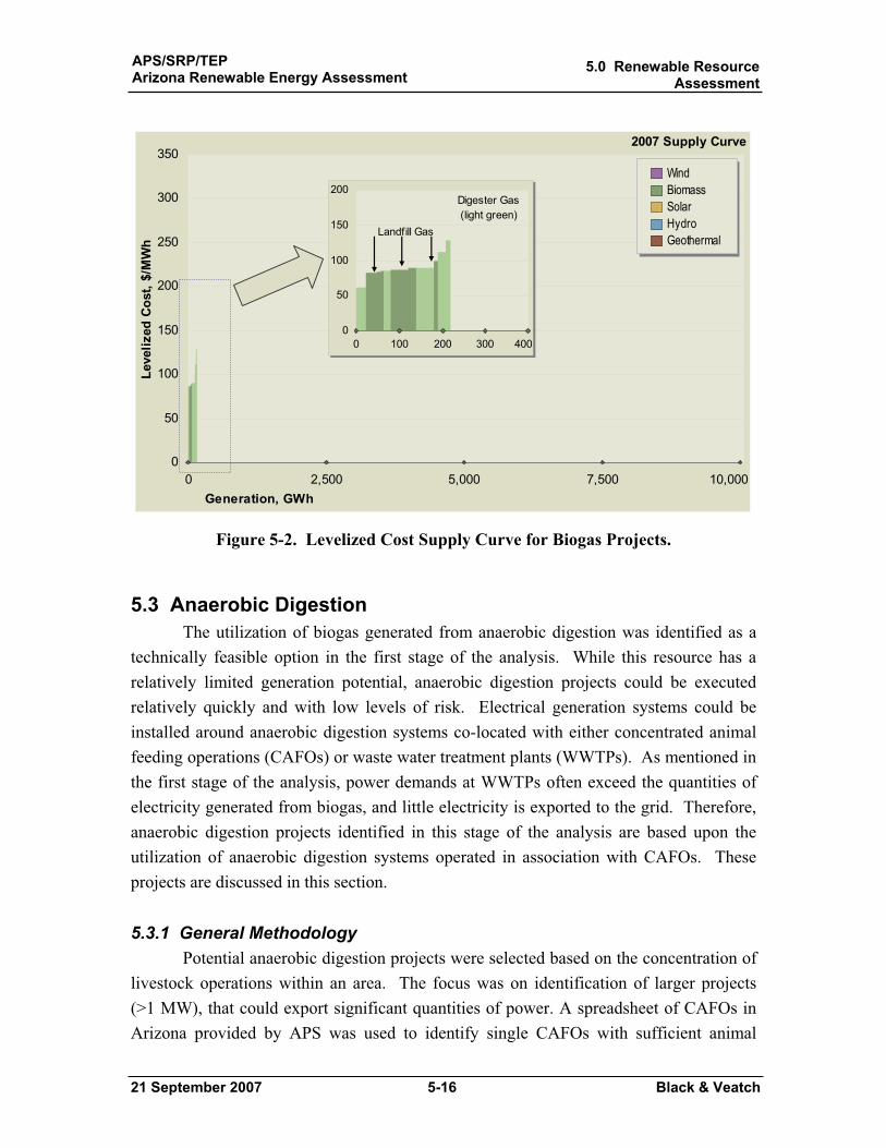
APS/SRP/TEPArizona Renewable Energy Assessment
5.0 Renewable ResourceAssessment
21 September 2007 5-16 Black & Veatch
0 2,500 5,000 7,500 10,0000
50
100
150
200
250
300
350
Generation, GWh
Leve
lized
Cos
t, $/
MW
h
WindBiomass SolarHydroGeothermal
2007 Supply Curve
0 100 200 300 4000
50
100
150
200Digester Gas(light green)
Landfill Gas
0 100 200 300 4000
50
100
150
200Digester Gas(light green)
Landfill Gas
Figure 5-2. Levelized Cost Supply Curve for Biogas Projects.
5.3 Anaerobic Digestion The utilization of biogas generated from anaerobic digestion was identified as a
technically feasible option in the first stage of the analysis. While this resource has a relatively limited generation potential, anaerobic digestion projects could be executed relatively quickly and with low levels of risk. Electrical generation systems could be installed around anaerobic digestion systems co-located with either concentrated animal feeding operations (CAFOs) or waste water treatment plants (WWTPs). As mentioned in the first stage of the analysis, power demands at WWTPs often exceed the quantities of electricity generated from biogas, and little electricity is exported to the grid. Therefore, anaerobic digestion projects identified in this stage of the analysis are based upon the utilization of anaerobic digestion systems operated in association with CAFOs. These projects are discussed in this section.
5.3.1 General Methodology Potential anaerobic digestion projects were selected based on the concentration of
livestock operations within an area. The focus was on identification of larger projects (>1 MW), that could export significant quantities of power. A spreadsheet of CAFOs in Arizona provided by APS was used to identify single CAFOs with sufficient animal
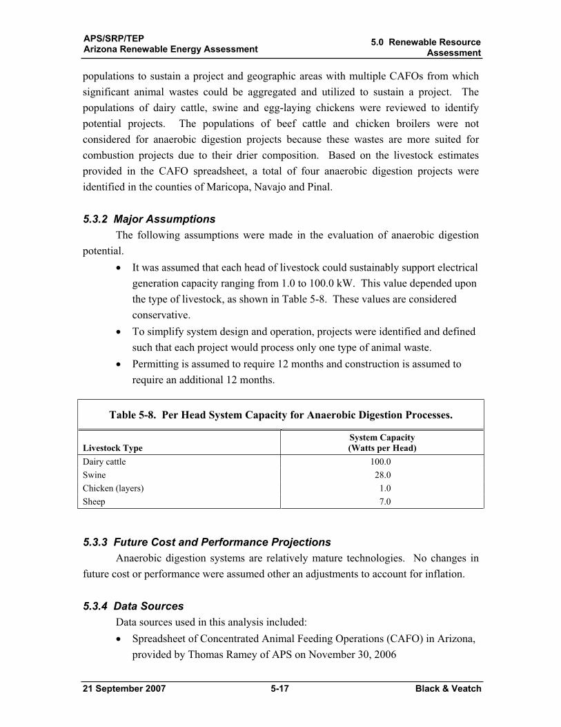
APS/SRP/TEPArizona Renewable Energy Assessment
5.0 Renewable ResourceAssessment
21 September 2007 5-17 Black & Veatch
populations to sustain a project and geographic areas with multiple CAFOs from which significant animal wastes could be aggregated and utilized to sustain a project. The populations of dairy cattle, swine and egg-laying chickens were reviewed to identify potential projects. The populations of beef cattle and chicken broilers were not considered for anaerobic digestion projects because these wastes are more suited for combustion projects due to their drier composition. Based on the livestock estimates provided in the CAFO spreadsheet, a total of four anaerobic digestion projects were identified in the counties of Maricopa, Navajo and Pinal.
5.3.2 Major Assumptions The following assumptions were made in the evaluation of anaerobic digestion
potential.It was assumed that each head of livestock could sustainably support electrical generation capacity ranging from 1.0 to 100.0 kW. This value depended upon the type of livestock, as shown in Table 5-8. These values are considered conservative.To simplify system design and operation, projects were identified and defined such that each project would process only one type of animal waste. Permitting is assumed to require 12 months and construction is assumed to require an additional 12 months.
Table 5-8. Per Head System Capacity for Anaerobic Digestion Processes.
Livestock Type System Capacity (Watts per Head)
Dairy cattle 100.0 Swine 28.0 Chicken (layers) 1.0 Sheep 7.0
5.3.3 Future Cost and Performance Projections Anaerobic digestion systems are relatively mature technologies. No changes in
future cost or performance were assumed other an adjustments to account for inflation.
5.3.4 Data Sources Data sources used in this analysis included:
Spreadsheet of Concentrated Animal Feeding Operations (CAFO) in Arizona, provided by Thomas Ramey of APS on November 30, 2006
APS/SRP/TEPArizona Renewable Energy Assessment
5.0 Renewable ResourceAssessment
21 September 2007 5-18 Black & Veatch
5.3.5 Projects Identified Four anaerobic digestion projects were identified:
A 3.5 MW swine manure digestion project located in Snowflake A 2.5 MW dairy cattle manure digestion project located in Buckeye A 1.5 MW dairy cattle manure digestion project located in Chandler A 2.4 MW poultry waste digestion project located in Maricopa
The swine manure project is proposed at Pigs for Farmer John (PFFJ) in Snowflake. The swine population of PFFJ is estimated to be 120,000 head, which could support approximately 3.5 MW of electrical generation. Assuming a capacity factor of 80 percent, this project could generate 25 GWh per year of electricity. It is assumed that this project would be located on the site of the hog operation, which will eliminate the cost of transporting manure to another location. It should be noted that Arizona voters in 2006 passed a proposition that will force this plant to change its animal management practices in the next few years. Local plant management has noted that plant closure is an option being considered. For this reason, there is some uncertainty regarding the viability of a renewable energy project at this site.
Two dairy manure projects are proposed in Maricopa County. The first project would be located in Buckeye and would produce 2.5 MW of electricity. Assuming a capacity factor of 80 percent, this facility would generate approximately 18 GWh per year of electricity. There are 29 dairy operations in Buckeye according to the CAFO spreadsheet, and the total size of the dairy population from these 29 operations is roughly 26,000 head. This population could support the entire 2.5 MW of generation proposed. However, there are also 14 dairy operations in Tolleson with over 15,000 head of cattle and additional operations in the vicinity to supplement the dairy manure resource.
The second dairy manure project would be located in Chandler and would produce 1.5 MW of electricity. Assuming a capacity factor of 80 percent, this facility would generate approximately 11 GWh per year of electricity. There are 17 dairy operations in Chandler, with another 10 operations in nearby Gilbert and Higley. The combined cattle population of these 27 operations is over 30,000 head, which is more than sufficient to provide the manure resources to provide 1.5 MW of capacity.
The chicken manure project would be located at Hickman’s Egg Ranch in Maricopa. The size of the Hickman operation is estimated at 2,400,000 chickens, and this population could support 2.4 MW of electrical generation. Assuming a capacity factor of 80 percent, this project could generate roughly 17 GWh per year of electricity. Because this project is supplied by manure from one location (similar to the swine
APS/SRP/TEPArizona Renewable Energy Assessment
5.0 Renewable ResourceAssessment
21 September 2007 5-19 Black & Veatch
manure project), the transportation cost of the manure will be significantly reduced, if not eliminated.
Given a notice to proceed of January 1, 2008, all of the proposed anaerobic digestion projects would likely be operational by January 1, 2010. The costs for the anaerobic digestion projects range from $70/MWh to $140/MWh (in 2010), largely dependent on project scale.
Table 5-9 shows the anaerobic digestion projects identified for this study. All characteristics are year 2007 values, before any future cost and performance modifications have been made. Figure 5-2 in the previous section shows the supply curve for anaerobic digestion gas generation potential (landfill gas projects are also shown). For the purposes of visualizing the projects on the supply curve, it has been assumed that all projects could be built in 2007. Appendix A shows a consolidated list of projects; Appendix B shows the same list with forecast levelized costs for each project from 2007 to 2025.
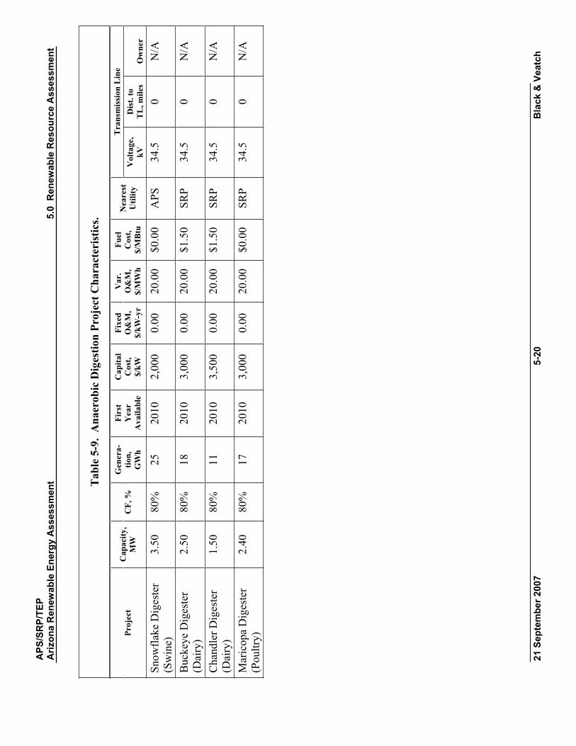
APS
/SR
P/TE
PA
rizon
a R
enew
able
Ene
rgy
Ass
essm
ent
5.0
Ren
ewab
le R
esou
rce
Ass
essm
ent
21 S
epte
mbe
r 200
7 5-
20
Bla
ck &
Vea
tch
Tab
le5-
9. A
naer
obic
Dig
estio
n Pr
ojec
t Cha
ract
eris
tics.
Tra
nsm
issi
on L
ine
Proj
ect
Cap
acity
, M
WC
F, %
G
ener
a-tio
n,G
Wh
Firs
tY
ear
Ava
ilabl
e
Cap
ital
Cos
t, $/
kW
Fixe
d O
&M
, $/
kW-y
r
Var
. O
&M
, $/
MW
h
Fuel
C
ost,
$/M
Btu
Nea
rest
U
tility
V
olta
ge,
kVD
ist.
to
TL
, mile
s O
wne
r
Snow
flake
Dig
este
r (S
win
e)3.
50
80%
25
20
10
2,00
0 0.
00
20.0
0 $0
.00
APS
34
.5
0 N
/A
Buc
keye
Dig
este
r (D
airy
)2.
50
80%
18
20
10
3,00
0 0.
00
20.0
0 $1
.50
SRP
34.5
0
N/A
Cha
ndle
r Dig
este
r (D
airy
)1.
50
80%
11
20
10
3,50
0 0.
00
20.0
0 $1
.50
SRP
34.5
0
N/A
Mar
icop
a D
iges
ter
(Pou
ltry)
2.
40
80%
17
20
10
3,00
0 0.
00
20.0
0 $0
.00
SRP
34.5
0
N/A
APS/SRP/TEPArizona Renewable Energy Assessment
5.0 Renewable ResourceAssessment
21 September 2007 5-21 Black & Veatch
5.4 Solar Thermal Electric The various solar thermal electric technologies were discussed in detail in
Section 4. One solar thermal electric technology, parabolic trough, is currently proven commercially, with over 350 MW operating in the Mohave Desert since about 1990, and with multiple plants of 50 MW or larger being constructed in the US and in Spain. This section will primarily focus on trough plants. Parabolic dish engine systems, for which there are power purchase agreements in California for hundreds of MWs, are unproven, but are treated as a special sensitivity case. Power tower and compact linear Fresnel reflector (CLFR) technologies hold potential, but are not included in this section because of uncertainty in cost and performance.
5.4.1 General Methodology The potential for solar thermal was characterized in a different manner than other
technologies. Whereas technologies such as biomass and geothermal are largely limited by resource availability, solar resources in Arizona are much larger than the potential near-term demand. Rather than being limited by resource, the technology is practically limited by equipment availability, development timelines, and ultimately economics. These factors were taken into account when forecasting potential solar thermal development.
The first parabolic trough plant was assumed to be a 100 MW facility with no thermal storage, but with hybrid fossil capability, which would go on line in 2011. Hybrid fossil capability means that the plant would have the ability to burn natural gas to generate electricity when the solar resource is unavailable.11 This design is identical to the operating solar trough plants in California. The size is consistent with first trough plants in planning. Subsequent plants would be 200 MW with levels of thermal storage as discussed later in this section.
Broad siting regions were identified rather than specific sites. A map of Arizona direct normal insolation overlaid with terrain constraints was obtained from the National Renewable Energy Laboratory (see Figure 4-19 in the previous chapter). This map was used to identify broad areas of interest. It should be noted that Arizona has vast areas which could be suitable for solar thermal electric plants. Generally, solar resource is quite high throughout the state, with terrain, transmission, and water availability being key constraints. For this study, terrain was considered via the NREL maps. It has been 11 In California, natural gas may be used for up to 25 percent of the facility output, without impacting the eligibility of the facility for renewable energy designation. For the purposes of this study, although the
APS/SRP/TEPArizona Renewable Energy Assessment
5.0 Renewable ResourceAssessment
21 September 2007 5-22 Black & Veatch
assumed that projects would be sited such that water for wet cooling would be available. Should water not be available, dry cooling would substantially lower water requirements, but would result in performance decreases and capital cost increases that would generally raise the cost of energy by about 10 percent.
Performance estimates have been based on Black & Veatch’s use of the NREL Excelergy model for Phoenix. Output was adjusted for direct normal insolation (DNI) estimates and latitude of the subject site. Excelergy estimates trough output on an hourly basis, estimating through collector field and power block thermal flows through the system, leading to net electrical output. Excelergy, which was developed by NREL, has been checked versus SEGS plant operation by NREL.
Phoenix output was modeled using Typical Meteorological Year (TMY2) data for Phoenix, along with the Phoenix latitude and longitude. Annual output for other sites was based on a comparison of satellite DNI for 0.1 degree latitude, 0.1 degree longitude pixels (about 5.7 miles east-west and 6.9 miles north-south in Arizona), and adjustment for latitude (trough output decreases with increase in latitude).
5.4.2 Major Assumptions Solar thermal development will be constrained in the near term due to the
practical limitations of the industry’s supply chain. Demand for solar thermal equipment and supporting engineering and construction services is at an unprecedented level worldwide. Due to these constraints, it has been assumed that the first 100 MW trough plant in Arizona could not be completed until 2011. Beginning in 2013, plants will be 200 MW to take advantage of economy of scale of larger plants. It is assumed that the near term supply chain constraints in the industry will be alleviated by 2013, and two to four 200 MW plants could be constructed per year thereafter.
Solar thermal plants need large amounts of contiguous land for a project. A 200 MW plant can require up to 1,400 acres. Securing such parcels of land with ideal terrain and transmission characteristics is sometimes difficult. As an example of the total amount of land that might be necessary for a large-scale solar expansion, Black & Veatch’s base case forecast estimates 2100 MW of solar trough development. Assuming a density of 7 acres/MW, this results in a need for 14,700 acres (23 square miles) of total land. By comparison, Phoenix proper covers an area of about 500 square miles.
The land used for solar thermal plants would likely be a mix of Arizona state land and BLM land. There is a bill currently proposed in congress designating “solar park” land for several GW of solar plants in the Southwest, with a lease fee of $200/acre/year.
facility is assumed capable of burning natural gas to provide a firm resource, no generation from gas was assumed.
APS/SRP/TEPArizona Renewable Energy Assessment
5.0 Renewable ResourceAssessment
21 September 2007 5-23 Black & Veatch
This may ease permitting requirements on federal lands. The Arizona land office is currently contemplating streamlined permitting requirements for solar parks. Private land is also an option, but it may be more expensive and more difficult to aggregate large contiguous parcels.
Unlike most other technologies evaluated for this study, it is expected that significant technical and cost advances will be realized for solar thermal trough plants. The initial plant available to be built in 2011 would be based on existing technology. This plant will have no thermal storage, but will have hybrid fossil capabilities. Plants built through 2016 will use current heat transfer fluid (HTF) technology: synthetic oil such as Therminol VP-1 or Dowtherm A. Beginning in 2017, plants are expected to use molten salt as the HTF to take advantage of higher temperatures, higher efficiencies, and cost savings. Moving to molten salt as the HTF will require technology and engineering advances. Such advances are consistent with industry projections.
Energy storage capability would be incorporated into plants beginning in 2013. Plants built in 2013 are assumed to have 3 hours of thermal storage. These plants would also have an increased solar multiple (larger solar field thermal output to turbine thermal input ratio), and thus larger mirror field, to accommodate longer operating hours using thermal storage. These plants would use synthetic oil as the HTF, with molten salt as the storage medium. This will require an oil-to-molten salt heat exchanger. Plants starting in 2014 are assumed to have 6 hours of thermal storage, increasing the operating hours and allowing increased dispatchability.
The following additional assumptions have been made in characterizing projects: Projects would be sited in areas with access to sufficient cooling water for wet cooling.Projects would be sited near existing transmission (a 230 kV substation with a 1 mile interconnect is assumed for all projects). Transmission constraints or the need for new transmission development have not been considered (similar to the remainder of the study).
5.4.3 Future Cost and Performance Projections Future cost and performance projections are shown in Table 5-10 for four
prospective sites. (Note that costs are in constant 2007$). The sites are discussed further in Section 5.4.5. Cost projections show the following trends, which can be somewhat off-setting.
Cost per kW increases with the addition of storage and increase of solar multiple.Cost per kW decreases with capacity increase from 100 MW to 200 MW.
APS/SRP/TEPArizona Renewable Energy Assessment
5.0 Renewable ResourceAssessment
21 September 2007 5-24 Black & Veatch
Costs decrease with time for the following reason. Increased deployment results in lower costs associated with perceived risk, with more efficient construction means. Increased competition by suppliers. More locally based manufacturing, and in particular, mirrors and receiver tubes decreasing shipping costs, import fees, and exchange rate issues. Improved technology, increasing efficiency and decreasing required mirror area.
Cost decreases have been estimated from data in Excelergy, the Western Governors Association report, the Sargent & Lundy report, and the Black & Veatch NREL report referenced in the next section.
Future performance projections include modest improvements with technology. These estimates were based on Excelergy model projections.
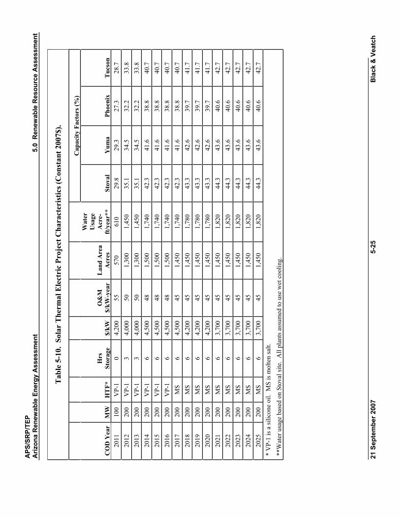
APS
/SR
P/TE
PA
rizon
a R
enew
able
Ene
rgy
Ass
essm
ent
5.0
Ren
ewab
le R
esou
rce
Ass
essm
ent
21 S
epte
mbe
r 200
7 5-
25
Bla
ck &
Vea
tch
Tab
le5-
10.
Sola
r T
herm
al E
lect
ric
Proj
ect C
hara
cter
istic
s (C
onst
ant 2
007$
).
C
apac
ity F
acto
rs (%
)
CO
D Y
ear
MW
H
TF*
H
rsSt
orag
e $/
kW
O&
M$/
kW-y
ear
Lan
d A
rea
Acr
es
Wat
erU
sage
Acr
e-ft
/yea
r**
Stov
al
Yum
a
Phoe
nix
T
ucso
n
2011
10
0 V
P-1
0 4,
200
55
570
610
29.8
29
.3
27.3
28
.7
2012
20
0 V
P-1
3 4,
000
50
1,30
0 1,
450
35.1
34
.5
32.2
33
.8
2013
20
0 V
P-1
3 4,
000
50
1,30
0 1,
450
35.1
34
.5
32.2
33
.8
2014
20
0 V
P-1
6 4,
500
48
1,50
0 1,
740
42.3
41
.6
38.8
40
.7
2015
20
0 V
P-1
6 4,
500
48
1,50
0 1,
740
42.3
41
.6
38.8
40
.7
2016
20
0 V
P-1
6 4,
500
48
1,50
0 1,
740
42.3
41
.6
38.8
40
.7
2017
20
0 M
S 6
4,50
0 45
1,
450
1,74
0 42
.3
41.6
38
.8
40.7
20
18
200
MS
6 4,
200
45
1,45
0 1,
780
43.3
42
.6
39.7
41
.7
2019
20
0 M
S 6
4,20
0 45
1,
450
1,78
0 43
.3
42.6
39
.7
41.7
20
20
200
MS
6 4,
200
45
1,45
0 1,
780
43.3
42
.6
39.7
41
.7
2021
20
0 M
S 6
3,70
0 45
1,
450
1,82
0 44
.3
43.6
40
.6
42.7
20
22
200
MS
6 3,
700
45
1,45
0 1,
820
44.3
43
.6
40.6
42
.7
2023
20
0 M
S 6
3,70
0 45
1,
450
1,82
0 44
.3
43.6
40
.6
42.7
20
24
200
MS
6 3,
700
45
1,45
0 1,
820
44.3
43
.6
40.6
42
.7
2025
20
0 M
S 6
3,70
0 45
1,
450
1,82
0 44
.3
43.6
40
.6
42.7
*
VP-
1 is
a si
licon
e oi
l. M
S is
mol
ten
salt.
**W
ater
usa
ge b
ased
on
Stov
al si
te.
All
plan
ts a
ssum
ed to
use
wet
coo
ling.
APS/SRP/TEPArizona Renewable Energy Assessment
5.0 Renewable ResourceAssessment
21 September 2007 5-26 Black & Veatch
5.4.4 Data Sources Cost data for the trough evaluation are based on several sources:
Black & Veatch Engineer, Procure, Construct bid price developed for confidential client, 2006.Preferred Plant Size, Bruce Kelly, Nexant, draft prepared for National Renewable Energy Laboratory, 2005-2006 Economic, Energy, and Environmental Benefits of Concentrating Solar Power in California, NREL/SR-550-39291, Black & Veatch, Prepared for National Renewable Energy Laboratory, April 2006.Assessment of Parabolic Trough and Power Tower Solar Technology Cost and Performance Forecasts, Sargent & Lundy Consulting Group, Prepared for Department of Energy and National Renewable Energy Laboratory (NREL), May 2003. Excelergy, Parabolic Trough Spreadsheet Model, developed by NREL. “Solar Task Force Report,” Western Governor’s Association, January 2006. Southwestern US DNI Satellite Data, spreadsheet obtained from NREL.Arizona DNI Map Overlaid with 1 Percent Slope, NREL website.
It should be noted that parabolic trough system costs are considerably higher than shown in many of the referenced documents. Costs of commodities, such as steel and copper, have risen significantly in the last two years. Furthermore, many of the trough components are manufactured in Europe, resulting in cost increases as the dollar has weakened compared to the euro.
5.4.5 Projects Identified Specific site locations were not identified at this stage of analysis. Generic
projects have been identified for four areas in Arizona: StovalYuma PhoenixTucson
Characteristics for these plants are shown in Table 5-11.The Stoval area, about 80 miles southwest of Phoenix along Interstate 8, has the
highest DNI of the potential sites (7.4 kwh/m2/day – per satellite data), with potential areas of low land slope. Because of the improved performance, it has been assumed that
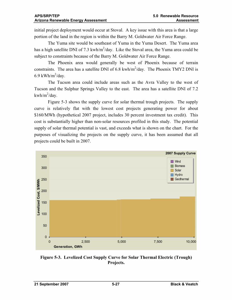
APS/SRP/TEPArizona Renewable Energy Assessment
5.0 Renewable ResourceAssessment
21 September 2007 5-27 Black & Veatch
initial project deployment would occur at Stoval. A key issue with this area is that a large portion of the land in the region is within the Barry M. Goldwater Air Force Range.
The Yuma site would be southeast of Yuma in the Yuma Desert. The Yuma area has a high satellite DNI of 7.3 kwh/m2/day. Like the Stoval area, the Yuma area could be subject to constraints because of the Barry M. Goldwater Air Force Range.
The Phoenix area would generally be west of Phoenix because of terrain constraints. The area has a satellite DNI of 6.8 kwh/m2/day. The Phoenix TMY2 DNI is 6.9 kWh/m2/day.
The Tucson area could include areas such as the Avra Valley to the west of Tucson and the Sulphur Springs Valley to the east. The area has a satellite DNI of 7.2 kwh/m2/day.
Figure 5-3 shows the supply curve for solar thermal trough projects. The supply curve is relatively flat with the lowest cost projects generating power for about $160/MWh (hypothetical 2007 project, includes 30 percent investment tax credit). This cost is substantially higher than non-solar resources profiled in this study. The potential supply of solar thermal potential is vast, and exceeds what is shown on the chart. For the purposes of visualizing the projects on the supply curve, it has been assumed that all projects could be built in 2007.
0 2,500 5,000 7,500 10,0000
50
100
150
200
250
300
350
Generation, GWh
Leve
lized
Cos
t, $/
MW
h
WindBiomass SolarHydroGeothermal
2007 Supply Curve
Figure 5-3. Levelized Cost Supply Curve for Solar Thermal Electric (Trough) Projects.
APS/SRP/TEPArizona Renewable Energy Assessment
5.0 Renewable ResourceAssessment
21 September 2007 5-28 Black & Veatch
5.4.6 Parabolic Dish Engine Assumptions At the present time, there are no operating commercial dish engine power plants.
There are, however, hundreds of megawatts of proposed projects which, if implemented successfully, would substantially advance the technology. For this reason, dish engine technology was not included in the base renewable energy development model (Section 7), but was included as a special sensitivity run. Stirling Engine Systems (SES), the principal dish engine developer in the United States, projects that the cost of dishes will decrease dramatically with hundreds of MWs of central station, grid connected deployment.
Cost and performance data (Table 5-11) for the dish engine systems were provided by SES, and represent a projection by SES of costs for 100 MW block system. Black & Veatch is unaware of any current independent cost estimates for parabolic dish Stirling systems. The estimate assumes significant deployment of dish systems, resulting in substantially lower capital costs than exist at present. The estimate also assumes that with the large deployment there are appropriate gains in system reliability.
The 100 MW system would comprise 4,000 x 25 kW dishes. The system would provide electricity in a sun-following mode, i.e., it would generate electricity when DNI is available and would not generate electricity at night or during cloud cover. The assumed capacity factor for dish systems at higher DNI sites in Arizona is 27.4 percent. Capacity factor will vary slightly depending on the site; however, this has not been included in the model.
Engineering, permitting, and other indirect costs are lower for dish engine plants than for parabolic trough plants. Trough plants require significant site-specific engineering compared to the far more modular dish systems.
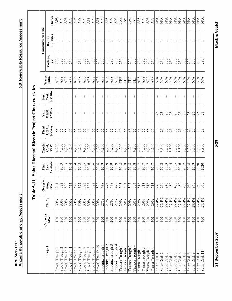
APS
/SR
P/TE
PA
rizon
a R
enew
able
Ene
rgy
Ass
essm
ent
5.0
Ren
ewab
le R
esou
rce
Ass
essm
ent
21 S
epte
mbe
r 200
7 5-
29
Bla
ck &
Vea
tch
Tab
le5-
11.
Sola
r T
herm
al E
lect
ric
Proj
ect C
hara
cter
istic
s.
Tra
nsm
issi
on L
ine
Proj
ect
Cap
acity
, M
WC
F, %
G
ener
a-tio
n,G
Wh
Firs
tY
ear
Ava
ilabl
e
Cap
ital
Cos
t, $/
kW
Fixe
d O
&M
, $/
kW-y
r
Var
. O
&M
, $/
MW
h
Fuel
C
ost,
$/M
Btu
Nea
rest
U
tility
V
olta
ge,
kVD
ist.
to
TL
, mile
s O
wne
r St
oval
Tro
ugh
1 10
0 30
%
261
2011
4,
200
55
– –
APS
23
0 1
APS
Stov
al T
roug
h 2
200
30%
52
2 20
13
4,20
0 55
–
– A
PS
230
1 A
PSSt
oval
Tro
ugh
3 20
0 30
%
522
2013
4,
200
55
– –
APS
23
0 1
APS
Stov
al T
roug
h 4
200
30%
52
2 20
14
4,20
0 55
–
– A
PS
230
1 A
PSSt
oval
Tro
ugh
5 20
0 30
%
522
2014
4,
200
55
– –
APS
23
0 1
APS
Stov
al T
roug
h 6
200
30%
52
2 20
15
4,20
0 55
–
– A
PS
230
1 A
PSSt
oval
Tro
ugh
7 20
0 30
%
522
2015
4,
200
55
– –
APS
23
0 1
APS
Stov
al T
roug
h 8
200
30%
52
2 20
16
4,20
0 55
–
– A
PS
230
1 A
PSSt
oval
Tro
ugh
9 20
0 30
%
522
2016
4,
200
55
– –
APS
23
0 1
APS
Stov
al T
roug
h 10
20
0 30
%
522
2016
4,
200
55
– –
APS
23
0 1
APS
Phoe
nix
Trou
gh 1
20
0 27
%
478
2019
4,
200
55
– –
APS
23
0 1
APS
Phoe
nix
Trou
gh 2
20
0 27
%
478
2019
4,
200
55
– –
APS
23
0 1
APS
Phoe
nix
Trou
gh 3
20
0 27
%
478
2019
4,
200
55
– –
APS
23
0 1
APS
Phoe
nix
Trou
gh 4
20
0 27
%
478
2019
4,
200
55
– –
APS
23
0 1
APS
Tucs
on T
roug
h 1
200
29%
50
3 20
18
4,20
0 55
–
– TE
P 23
0 1
Loca
lTu
cson
Tro
ugh
2 20
0 29
%
503
2018
4,
200
55
– –
TEP
230
1 Lo
cal
Tucs
on T
roug
h 3
200
29%
50
3 20
18
4,20
0 55
–
– TE
P 23
0 1
Loca
lTu
cson
Tro
ugh
4 20
0 29
%
503
2018
4,
200
55
– –
TEP
230
1 Lo
cal
Yum
a Tr
ough
1
200
29%
51
3 20
17
4,20
0 55
–
– A
PS
230
1 A
PSY
uma
Trou
gh 2
20
0 29
%
513
2017
4,
200
55
– –
APS
23
0 1
APS
Yum
a Tr
ough
3
200
29%
51
3 20
17
4,20
0 55
–
– A
PS
230
1 A
PSY
uma
Trou
gh 4
20
0 29
%
513
2017
4,
200
55
– –
APS
23
0 1
APS
Sola
r Dis
h 1
100
27.4
%
240
2011
3,
300
23
25
– N
/A
230
1 N
/A
Sola
r Dis
h 2
100
27.4
%
240
2012
3,
300
23
25
– N
/A
230
1 N
/A
Sola
r Dis
h 3
100
27.4
%
240
2013
3,
300
23
25
– N
/A
230
1 N
/A
Sola
r Dis
h 4
200
27.4
%
480
2014
3,
300
23
25
– N
/A
230
1 N
/A
Sola
r Dis
h 5
200
27.4
%
480
2015
3,
300
23
25
– N
/A
230
1 N
/A
Sola
r Dis
h 6
200
27.4
%
480
2016
3,
300
23
25
– N
/A
230
1 N
/A
Sola
r Dis
h 7
400
27.4
%
960
2017
3,
300
23
25
– N
/A
230
1 N
/A
Sola
r Dis
h 8
400
27.4
%
960
2018
3,
300
23
25
– N
/A
230
1 N
/A
Sola
r Dis
h 9
400
27.4
%
960
2019
3,
300
23
25
– N
/A
230
1 N
/A
Sola
r Dis
h 10
40
0 27
.4%
96
0 20
20
3,30
0 23
25
–
N/A
23
0 1
N/A
So
lar D
ish
11
400
27.4
%
960
2020
3,
300
23
25
– N
/A
230
1 N
/A
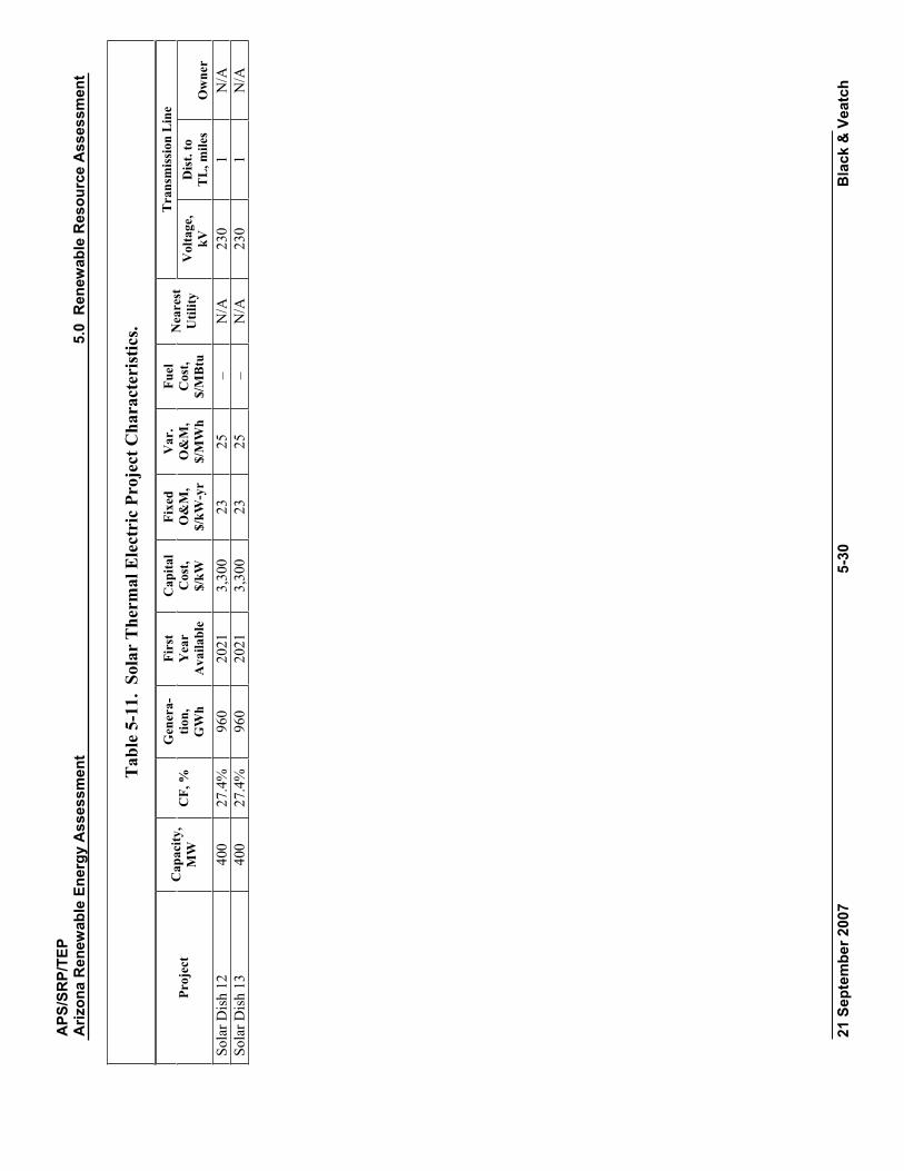
APS
/SR
P/TE
PA
rizon
a R
enew
able
Ene
rgy
Ass
essm
ent
5.0
Ren
ewab
le R
esou
rce
Ass
essm
ent
21 S
epte
mbe
r 200
7 5-
30
Bla
ck &
Vea
tch
Tab
le5-
11.
Sola
r T
herm
al E
lect
ric
Proj
ect C
hara
cter
istic
s.
Tra
nsm
issi
on L
ine
Proj
ect
Cap
acity
, M
WC
F, %
G
ener
a-tio
n,G
Wh
Firs
tY
ear
Ava
ilabl
e
Cap
ital
Cos
t, $/
kW
Fixe
d O
&M
, $/
kW-y
r
Var
. O
&M
, $/
MW
h
Fuel
C
ost,
$/M
Btu
Nea
rest
U
tility
V
olta
ge,
kVD
ist.
to
TL
, mile
s O
wne
r So
lar D
ish
12
400
27.4
%
960
2021
3,
300
23
25
– N
/A
230
1 N
/A
Sola
r Dis
h 13
40
0 27
.4%
96
0 20
21
3,30
0 23
25
–
N/A
23
0 1
N/A
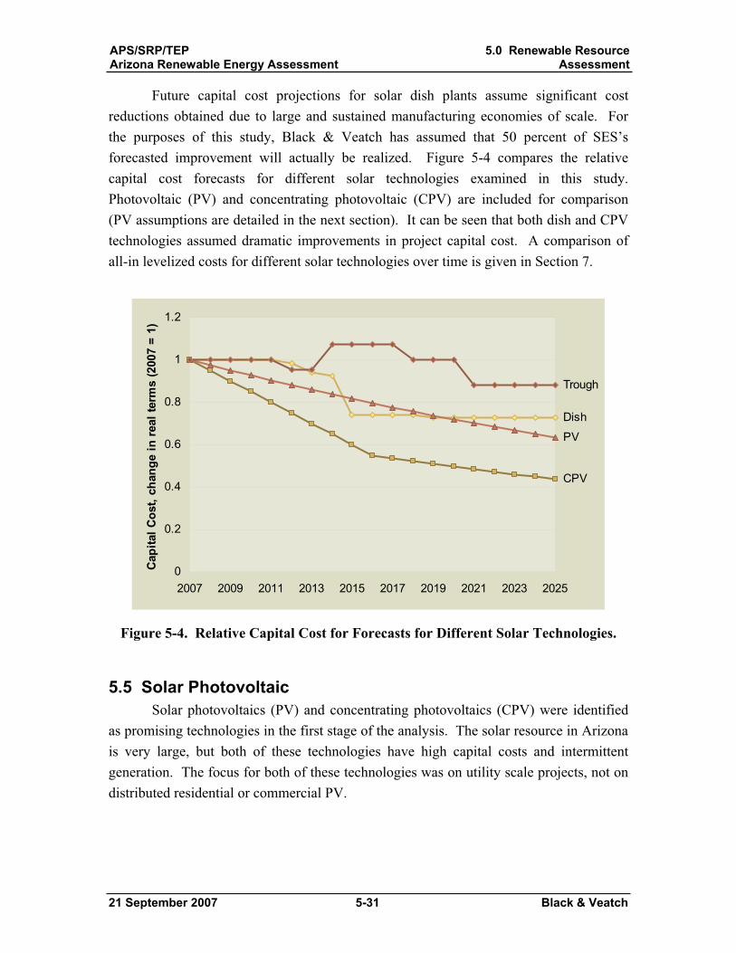
APS/SRP/TEPArizona Renewable Energy Assessment
5.0 Renewable ResourceAssessment
21 September 2007 5-31 Black & Veatch
Future capital cost projections for solar dish plants assume significant cost reductions obtained due to large and sustained manufacturing economies of scale. For the purposes of this study, Black & Veatch has assumed that 50 percent of SES’s forecasted improvement will actually be realized. Figure 5-4 compares the relative capital cost forecasts for different solar technologies examined in this study. Photovoltaic (PV) and concentrating photovoltaic (CPV) are included for comparison (PV assumptions are detailed in the next section). It can be seen that both dish and CPV technologies assumed dramatic improvements in project capital cost. A comparison of all-in levelized costs for different solar technologies over time is given in Section 7.
Dish
CPV
PV
Trough
0
0.2
0.4
0.6
0.8
1
1.2
2007 2009 2011 2013 2015 2017 2019 2021 2023 2025
Cap
ital C
ost,
chan
ge in
real
term
s (2
007
= 1)
Figure 5-4. Relative Capital Cost for Forecasts for Different Solar Technologies.
5.5 Solar Photovoltaic Solar photovoltaics (PV) and concentrating photovoltaics (CPV) were identified
as promising technologies in the first stage of the analysis. The solar resource in Arizona is very large, but both of these technologies have high capital costs and intermittent generation. The focus for both of these technologies was on utility scale projects, not on distributed residential or commercial PV.

APS/SRP/TEPArizona Renewable Energy Assessment
5.0 Renewable ResourceAssessment
21 September 2007 5-32 Black & Veatch
5.5.1 General Methodology As discussed in the previous section, solar is a special case because the resource is
generally available anywhere in the state; the constraints in solar are mainly capital costs and equipment availability. PV and CPV use little water, and projects were assumed to be in the 5-10 MW range, requiring 50-100 acres of land and minimal transmission capacity. Resource, transmission and land were assumed to be available for PV and CPV development. The approach was to make assumptions about future capital costs and the equipment available for utility scale projects.
5.5.2 Major Assumptions The following assumptions were made in the evaluation of solar photovoltaic
potential.Siting for PV or CPV projects is not a major constraint, due to modest land requirements and low environmental impact. PV projects will be up to 10 MW in any given location through 2015, allowing interconnection to distribution networks or low voltage transmission. We would expect larger plants after that time if economics are viable.
5.5.3 Future Cost and Performance Projections Black & Veatch feels traditional flat plate for utility scale will see modest cost
reduction in the near term. Utility scale PV has limited economies of scale, and module costs make up a large portion of total capital costs. Current capital costs for utility scale PV in the US are around $6,000/kWp, and there is little room for future improvement in non-module costs such as inverters and wiring. While there are promising developments in thin-film PV and non-silicon materials, these modules may be better suited for the distributed PV market. Most current utility scale PV projects are using traditional silicon materials due to concerns about degradation and the life of thin-film modules. Black & Veatch assumed that PV costs would remain flat in nominal dollars for the indefinite future. This translates to a 2.5 percent annual decrease in real dollars.
Concentrating PV was seen as more promising for cost reductions in utility applications. Concentrating PV uses far less silicon than traditional PV, and high efficiency chips are more cost-effective in CPV applications. Spectrolab, a Boeing subsidiary and a leader in high performance triple-junction solar cells, recently crossed the 40 percent efficiency barrier. Concentrating PV is still an immature industry, which makes cost reductions more likely. Mass production of lenses and tracking components could bring costs down over the next decade. There are a number of companies addressing concentrating PV, including Amonix, Sharp, Sol Focus, Green Volts, and
APS/SRP/TEPArizona Renewable Energy Assessment
5.0 Renewable ResourceAssessment
21 September 2007 5-33 Black & Veatch
others. Many of these companies have been recently funded by venture capital and are currently developing products.
Black & Veatch assumed capital costs for CPV would decrease in real dollars by approximately 5 percent annually, maturing in 2016 at 55 percent of current costs (a 5 MW CPV plant would drop from $7,200/kWp to $3,960/kWp in 2016). Capacity factors would remain unchanged.
Figure 5-4 in the previous section compares the relative capital cost forecasts for different solar technologies examined in this study. A comparison of all-in levelized costs for different solar technologies over time is given in Section 7.
5.5.4 Data Sources Data sources used in this analysis included:
Black & Veatch Independent Engineering report for utility scale PV and CPV plant, confidential client, March 2007. Western Governor’s Association, Clean and Diversified Energy Initiative, “Solar Task Force Report” January 2006. Available at http://www.westgov.org/wga/initiatives/cdeac/solar.htm Maycock, Paul. “PV Market Update” Renewable Energy World, July-August 2005Navigant Consulting, “Arizona Solar Electric Roadmap Study” prepared for the Arizona Department of Commerce, January 2007. Available at http://www.azcommerce.com/doclib/energy/az_solar_electric_roadmap_study_full_report.pdfWiser, Ryan et al “Letting the Sun Shine on Solar Costs: An Empirical Investigation of Photovoltaic Cost Trends in California” LBNL January 2006. Available at http://eetd.lbl.gov/EA/EMP “The US Photovoltaic Industry Roadmap,” Available at http://www.sandia.gov/pv/docs/PVRMPV_Road_Map.htm Western Governor’s Association, Clean and Diversified Energy Initiative, “Solar Task Force Report” January 2006. Available at http://www.westgov.org/wga/initiatives/cdeac/solar.htm
5.5.5 Projects Identified Most flat plate PV is sensitive to temperature and insolation, which varies
capacity factors across the state. PV, especially crystalline silicon used in most utility scale PV projects, performs best in areas of low temperatures and high insolation, such as TEP’s Springerville plant or APS’s Prescott plant. For flat plate PV, Black & Veatch
APS/SRP/TEPArizona Renewable Energy Assessment
5.0 Renewable ResourceAssessment
21 September 2007 5-34 Black & Veatch
assumed a typical 5 MWp plant, either a fixed installation (such as Springerville) or with single axis tracking (Prescott). Capital costs shown are $/kWp and do not include the federal 30 percent ITC. Capital costs are from current utility scale PV projects. Black & Veatch used PV simulation software to estimate the capacity factors for four locations in the state: Prescott, Tucson, Phoenix and Flagstaff. The software takes insolation and temperature into account to generate capacity factors.
While the main limits to PV are cost, there are also limitations in the global supply chain for PV modules. Black & Veatch assumed that 15 MW were available for utility scale projects in Arizona for 2008 and 2009, ramping up to 500 MW in 2010 and later. However, because of the high cost of solar photovoltaics, larger projects are not forecast to be built.
Concentrating PV is less sensitive to ambient temperature, as the solar modules are designed to withstand higher temperatures, and CPV systems typically include heat rejection. Concentrating PV has a higher capacity factor than flat plate PV due to increased cell efficiency and the use of dual-axis tracking. Concentrating PV, like solar thermal technologies, use direct normal insolation (DNI). The best locations for CPV are therefore similar to the locations for solar thermal. Black & Veatch did not specify individual sites for CPV, due to the small size of projects and the lack of resource and transmission constraints.
Because of the immaturity of the industry, there are limitations to the amount of concentrating PV systems that can be installed in any given year. CPV is also capital intensive – 100 MW of CPV represents a $500 million investment. In addition, PV industry is a global industry and other markets (Germany, Japan, California) will place demands on the global supply. Black & Veatch assumed the following ramp up of the industry
1 MW of CPV could be installed in 2008 A single 5 MW CPV plant could be installed in 2009 Two 5 MW CPV plants (10 MW total) could be installed in 2010 Two 10 MW CPV plants (20 MW total) could be installed in 2011 Four 10 MW CPV plants (20 MW total) could be installed in 2012 Ten 10 MW CPV plants (100 MW total) could be installed in 2013-2015
Figure 5-5 shows the supply curve for PV projects. The curve does not include CPV projects, but they are considered in Section 8.
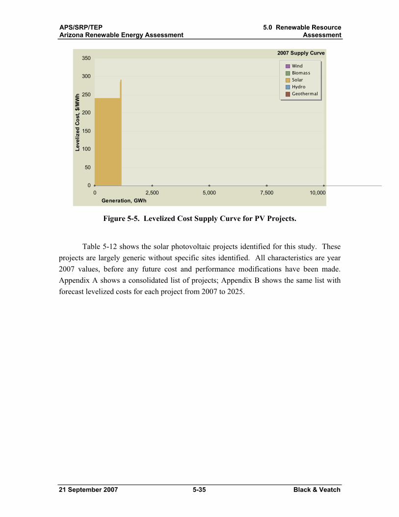
APS/SRP/TEPArizona Renewable Energy Assessment
5.0 Renewable ResourceAssessment
21 September 2007 5-35 Black & Veatch
0 2,500 5,000 7,500 10,0000
50
100
150
200
250
300
350
Generation, GWh
Leve
lized
Cos
t, $/
MW
h
WindBiomass SolarHydroGeothermal
2007 Supply Curve
Figure 5-5. Levelized Cost Supply Curve for PV Projects.
Table 5-12 shows the solar photovoltaic projects identified for this study. These projects are largely generic without specific sites identified. All characteristics are year 2007 values, before any future cost and performance modifications have been made. Appendix A shows a consolidated list of projects; Appendix B shows the same list with forecast levelized costs for each project from 2007 to 2025.
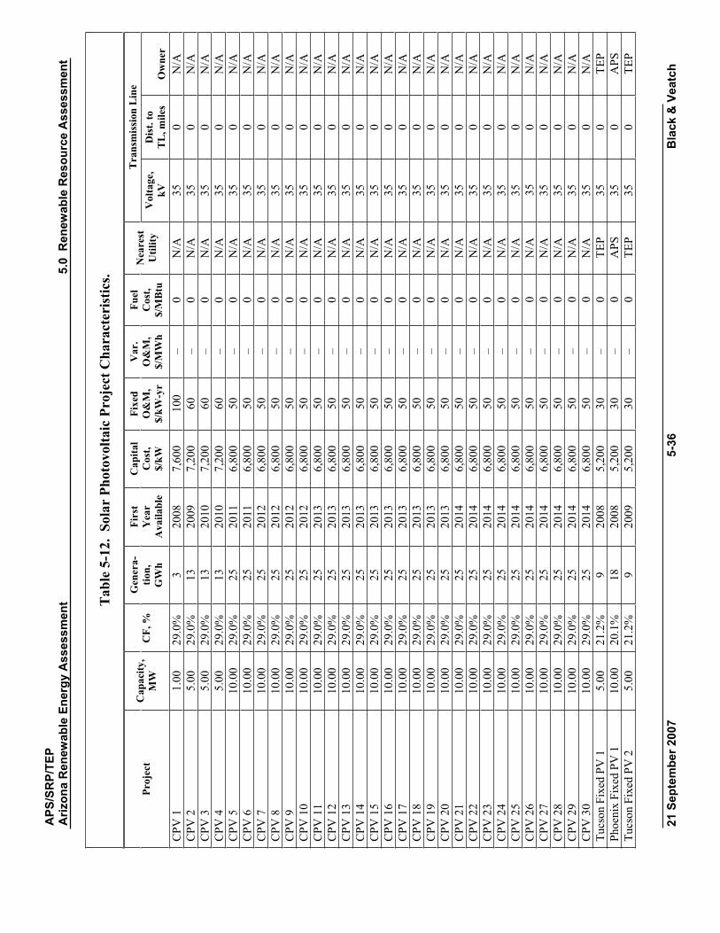
APS
/SR
P/TE
PA
rizon
a R
enew
able
Ene
rgy
Ass
essm
ent
5.0
Ren
ewab
le R
esou
rce
Ass
essm
ent
21 S
epte
mbe
r 200
7 5-
36
Bla
ck &
Vea
tch
Tab
le5-
12.
Sola
r Ph
otov
olta
ic P
roje
ct C
hara
cter
istic
s.
Tra
nsm
issi
on L
ine
Proj
ect
Cap
acity
, M
WC
F, %
G
ener
a-tio
n,G
Wh
Firs
tY
ear
Ava
ilabl
e
Cap
ital
Cos
t, $/
kW
Fixe
d O
&M
, $/
kW-y
r
Var
. O
&M
, $/
MW
h
Fuel
C
ost,
$/M
Btu
Nea
rest
U
tility
V
olta
ge,
kVD
ist.
to
TL
, mile
s O
wne
r C
PV 1
1.
00
29.0
%
3 20
08
7,60
0 10
0 –
0 N
/A
35
0 N
/A
CPV
2
5.00
29
.0%
13
20
09
7,20
0 60
–
0 N
/A
35
0 N
/A
CPV
3
5.00
29
.0%
13
20
10
7,20
0 60
–
0 N
/A
35
0 N
/A
CPV
4
5.00
29
.0%
13
20
10
7,20
0 60
–
0 N
/A
35
0 N
/A
CPV
5
10.0
0 29
.0%
25
20
11
6,80
0 50
–
0 N
/A
35
0 N
/A
CPV
6
10.0
0 29
.0%
25
20
11
6,80
0 50
–
0 N
/A
35
0 N
/A
CPV
7
10.0
0 29
.0%
25
20
12
6,80
0 50
–
0 N
/A
35
0 N
/A
CPV
8
10.0
0 29
.0%
25
20
12
6,80
0 50
–
0 N
/A
35
0 N
/A
CPV
9
10.0
0 29
.0%
25
20
12
6,80
0 50
–
0 N
/A
35
0 N
/A
CPV
10
10.0
0 29
.0%
25
20
12
6,80
0 50
–
0 N
/A
35
0 N
/A
CPV
11
10.0
0 29
.0%
25
20
13
6,80
0 50
–
0 N
/A
35
0 N
/A
CPV
12
10.0
0 29
.0%
25
20
13
6,80
0 50
–
0 N
/A
35
0 N
/A
CPV
13
10.0
0 29
.0%
25
20
13
6,80
0 50
–
0 N
/A
35
0 N
/A
CPV
14
10.0
0 29
.0%
25
20
13
6,80
0 50
–
0 N
/A
35
0 N
/A
CPV
15
10.0
0 29
.0%
25
20
13
6,80
0 50
–
0 N
/A
35
0 N
/A
CPV
16
10.0
0 29
.0%
25
20
13
6,80
0 50
–
0 N
/A
35
0 N
/A
CPV
17
10.0
0 29
.0%
25
20
13
6,80
0 50
–
0 N
/A
35
0 N
/A
CPV
18
10.0
0 29
.0%
25
20
13
6,80
0 50
–
0 N
/A
35
0 N
/A
CPV
19
10.0
0 29
.0%
25
20
13
6,80
0 50
–
0 N
/A
35
0 N
/A
CPV
20
10.0
0 29
.0%
25
20
13
6,80
0 50
–
0 N
/A
35
0 N
/A
CPV
21
10.0
0 29
.0%
25
20
14
6,80
0 50
–
0 N
/A
35
0 N
/A
CPV
22
10.0
0 29
.0%
25
20
14
6,80
0 50
–
0 N
/A
35
0 N
/A
CPV
23
10.0
0 29
.0%
25
20
14
6,80
0 50
–
0 N
/A
35
0 N
/A
CPV
24
10.0
0 29
.0%
25
20
14
6,80
0 50
–
0 N
/A
35
0 N
/A
CPV
25
10.0
0 29
.0%
25
20
14
6,80
0 50
–
0 N
/A
35
0 N
/A
CPV
26
10.0
0 29
.0%
25
20
14
6,80
0 50
–
0 N
/A
35
0 N
/A
CPV
27
10.0
0 29
.0%
25
20
14
6,80
0 50
–
0 N
/A
35
0 N
/A
CPV
28
10.0
0 29
.0%
25
20
14
6,80
0 50
–
0 N
/A
35
0 N
/A
CPV
29
10.0
0 29
.0%
25
20
14
6,80
0 50
–
0 N
/A
35
0 N
/A
CPV
30
10.0
0 29
.0%
25
20
14
6,80
0 50
–
0 N
/A
35
0 N
/A
Tucs
on F
ixed
PV
1
5.00
21
.2%
9
2008
5,
200
30
– 0
TEP
35
0 TE
P Ph
oeni
x Fi
xed
PV 1
10
.00
20.1
%
18
2008
5,
200
30
– 0
APS
35
0
APS
Tu
cson
Fix
ed P
V 2
5.
00
21.2
%
9 20
09
5,20
0 30
–
0 TE
P 35
0
TEP
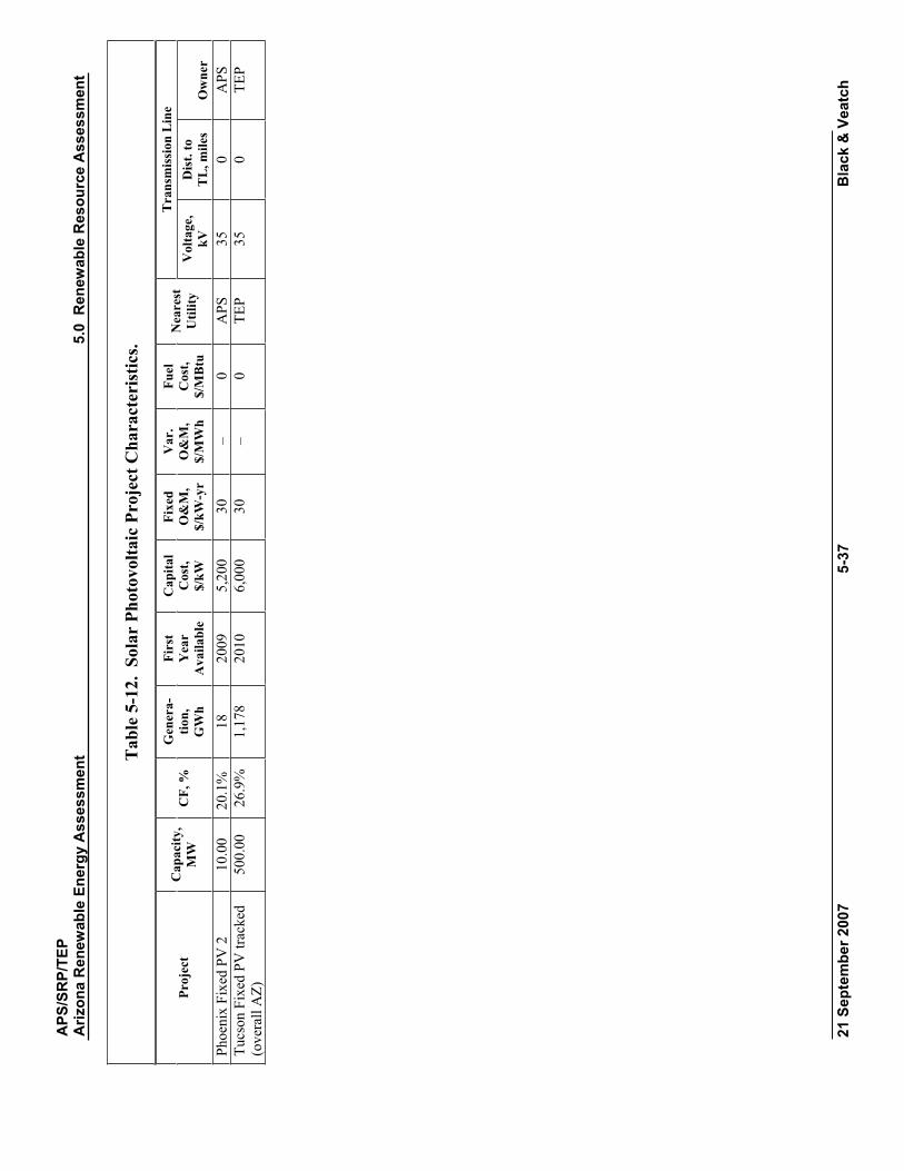
APS
/SR
P/TE
PA
rizon
a R
enew
able
Ene
rgy
Ass
essm
ent
5.0
Ren
ewab
le R
esou
rce
Ass
essm
ent
21 S
epte
mbe
r 200
7 5-
37
Bla
ck &
Vea
tch
Tab
le5-
12.
Sola
r Ph
otov
olta
ic P
roje
ct C
hara
cter
istic
s.
Tra
nsm
issi
on L
ine
Proj
ect
Cap
acity
, M
WC
F, %
G
ener
a-tio
n,G
Wh
Firs
tY
ear
Ava
ilabl
e
Cap
ital
Cos
t, $/
kW
Fixe
d O
&M
, $/
kW-y
r
Var
. O
&M
, $/
MW
h
Fuel
C
ost,
$/M
Btu
Nea
rest
U
tility
V
olta
ge,
kVD
ist.
to
TL
, mile
s O
wne
r Ph
oeni
x Fi
xed
PV 2
10
.00
20.1
%
18
2009
5,
200
30
– 0
APS
35
0
APS
Tu
cson
Fix
ed P
V tr
acke
d (o
vera
ll A
Z)
500.
00
26.9
%
1,17
8 20
10
6,00
0 30
–
0 TE
P 35
0
TEP
APS/SRP/TEPArizona Renewable Energy Assessment 5.0 Renewable Resource Assessment
21 September 2007 5-38 Black & Veatch
5.6 Hydroelectric Black & Veatch reviewed hydroelectric options that included power production
options from man-made water flows, improvements at existing facilities, new sites and pumped storage for load management. This assessment is based on projects previously identified as promising in the Interim Report (Section 4). Seven projects were identified for further investigation
5.6.1 General Methodology Black & Veatch identified seven hydroelectric projects for characterization and an
additional seven pumped storage projects. The overall number of projects were limited to these based on water resource availability and environmental concerns.
5.6.2 Major Assumptions There are a variety of methods to estimate performance of proposed hydroelectric
projects. One useful method of estimating plant performance is to review generation records. Except for the Glen Canyon project, power generation records for the existing hydroelectric facilities were not available for review for this study. Flow duration curves can also be used to estimate performance; however, these were not available either. For this study 40 percent capacity factor was assumed for the smaller hydroelectric projects. This percentage was based on Black & Veatch experience with projects of these characteristics. Forty-five percent was assumed for Glen Canyon dam which is classified as medium hydroelectric project. Without specific site layouts it is impossible to determine a site specific capacity factor. Therefore the capacity factors in the model are estimates only.
A nationwide database of hydroelectric construction cost information per kW of capacity is available from the Department of Energy. In 2003, the nationwide average to develop a hydroelectric project ranged from about $500-6,000/kW, with a median about $2,700/kW for an undeveloped site, and $700/kW for upgrade projects at sites with existing generation. As would be expected, specific costs decrease with plant size and previous development of the site. Most of the selected projects fit within this range.
Like wind and solar, capital costs for hydroelectric projects make up most of the overall costs since the “fuel” is “free” once the required infrastructure is in place. For hydroelectric projects, much of the cost is often off-site from the power plant in the diversion structures, penstock, and their associated access roads. The variability in project site requirements leads to broad ranges of potential costs. For this reason, it is
APS/SRP/TEPArizona Renewable Energy Assessment 5.0 Renewable Resource Assessment
21 September 2007 5-39 Black & Veatch
difficult to develop generic estimates of project costs without detailed site studies, and past detailed estimates, despite their age, are preferred.
Project O&M costs are estimated based on percent of construction cost and staff allocation. O&M costs are expected to be higher for upgrade plants because, though some of the equipment would be new, the diversion and conveyance structures may still require a greater level of maintenance than a new project.
Hydroelectric projects are expected to take longer to develop than other renewable energy projects. Except for Glen Canyon, all the projects identified in this report assume installation by 2013. The Glen Canyon addition is assumed to not be complete until 2015.
5.6.3 Future Cost and Performance Projections Hydroelectric power generation and hydroelectric pumped storage are largely
mature technologies. No changes in future cost or performance were assumed other than adjustments to account for inflation.
5.6.4 Data Sources Data sources used in this analysis included:
U.S. Hydropower Resource Assessment for Arizona, Rinehart, Ben, Conner, Alison and Francfort, James, October 1997, Idaho National Engineering and Environmental Laboratory, and Renewable Energy Products Department, Lockheed Martin Idaho Technologies Company, http://hydropower.inel.gov/resourceassessment/pdfs/states/az.pdf. Telephone conversations with Doug Hall, Program Manager for INL Hydropower Program. Contacts with individual site owners, as possible.
5.6.5 Projects Identified This section provides descriptions of seven hydroelectric projects identified
previously in Section 4. These projects have been previously identified and studied by the Idaho National Laboratory (INL), previously INEEL, the Idaho National Engineering and Environmental Laboratory. Six of the seven project sites are located in the southern portion of the state and have a relatively small capacity in comparison to the total capacity of hydroelectric in the state.
Using the INL database as a starting point, this study included a further detailed search of public records on the internet, contacting the reported owners of each of the projects, and contacting Doug Hall who is the current program manager for the INL
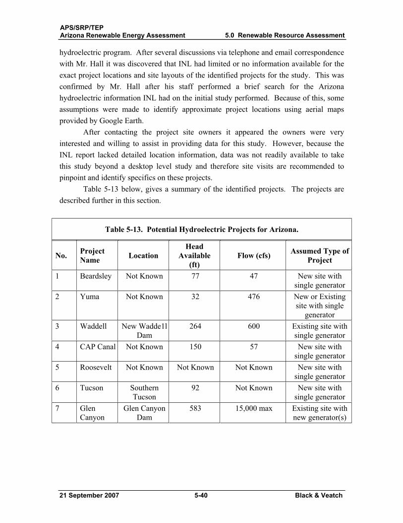
APS/SRP/TEPArizona Renewable Energy Assessment 5.0 Renewable Resource Assessment
21 September 2007 5-40 Black & Veatch
hydroelectric program. After several discussions via telephone and email correspondence with Mr. Hall it was discovered that INL had limited or no information available for the exact project locations and site layouts of the identified projects for the study. This was confirmed by Mr. Hall after his staff performed a brief search for the Arizona hydroelectric information INL had on the initial study performed. Because of this, some assumptions were made to identify approximate project locations using aerial maps provided by Google Earth.
After contacting the project site owners it appeared the owners were very interested and willing to assist in providing data for this study. However, because the INL report lacked detailed location information, data was not readily available to take this study beyond a desktop level study and therefore site visits are recommended to pinpoint and identify specifics on these projects.
Table 5-13 below, gives a summary of the identified projects. The projects are described further in this section.
Table 5-13. Potential Hydroelectric Projects for Arizona.
No. ProjectName Location
HeadAvailable
(ft)Flow (cfs) Assumed Type of
Project
1 Beardsley Not Known 77 47 New site with single generator
2 Yuma Not Known 32 476 New or Existing site with single
generator3 Waddell New Wadde1l
Dam 264 600 Existing site with
single generator 4 CAP Canal Not Known 150 57 New site with
single generator 5 Roosevelt Not Known Not Known Not Known New site with
single generator 6 Tucson Southern
Tucson92 Not Known New site with
single generator 7 Glen
CanyonGlen Canyon
Dam 583 15,000 max Existing site with
new generator(s)
APS/SRP/TEPArizona Renewable Energy Assessment 5.0 Renewable Resource Assessment
21 September 2007 5-41 Black & Veatch
Beardsley Canal Drop Information provided by INL and public records do not give the precise location
or details of the Beardsley canal drop project. The estimated Beardsley Canal project site is located approximately 26 miles from Phoenix, Arizona with overhead power owned by Arizona Public Service available along the presumed project location. The average flowrate in the canal is estimated at 47 cubic feet per second (cfs) with a hydraulic head of 77 feet (ft). Since the information provided on the location of this project can not reasonably pinpoint the project site location it is unclear how to take advantage of the 77 ft of hydraulic head. A local drop in the canal might make it attractive as an open flume, however the hydraulics of this situation with the energy extraction at the powerhouse, would create a sizeable tailwater pool. Further study would be necessary to locate a local drop.
Yuma Main Canal The locations from the INL database do not clearly identify the location or details
of the Yuma Main Canal project. Coordinates listed by INL show the location near the canal. The estimated Yuma Main Canal project site is located approximately 140 miles from Phoenix, with overhead power owned by the Department of Energy available along the presumed project location. Hydraulic head for this site is 32 ft and the flow rate for this site is estimated at 476 cfs. The flow rate is quite large for a canal indicating that a location at the end of a canal run is questionable. Further research uncovered an existing siphon-drop power plant located along the Yuma Main Canal located near Yuma, Arizona. The new power plant began operation in 1987, replacing an earlier power plant located 500 ft downstream that ended operation in 1972. Further study would be necessary to identify this project as a new site or simply an upgrade to the existing power plant.
WaddellThe locations from the INL database do not clearly identify the location or details
of the Waddell project. Coordinates listed by INL show the location near the New Waddell Dam. New Waddell Dam is located approximately 30 miles from Phoenix and is located at the New Lake Pleasant Reservoir. The U.S. States Department of the Interior website listed New Waddell Dam as not currently having power generation at the site. However further research uncovered an existing hydroelectric facility in operation. The outlet works capacity is listed at 600 cfs and has a hydraulic head of approximately 264 ft. It is assumed that this project would consist of adding a generator at the existing power plant at New Waddell Dam.
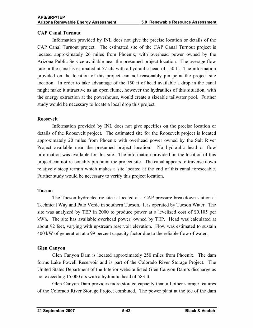
APS/SRP/TEPArizona Renewable Energy Assessment 5.0 Renewable Resource Assessment
21 September 2007 5-42 Black & Veatch
CAP Canal Turnout Information provided by INL does not give the precise location or details of the
CAP Canal Turnout project. The estimated site of the CAP Canal Turnout project is located approximately 26 miles from Phoenix, with overhead power owned by the Arizona Public Service available near the presumed project location. The average flow rate in the canal is estimated at 57 cfs with a hydraulic head of 150 ft. The information provided on the location of this project can not reasonably pin point the project site location. In order to take advantage of the 150 ft of head available a drop in the canal might make it attractive as an open flume, however the hydraulics of this situation, with the energy extraction at the powerhouse, would create a sizeable tailwater pool. Further study would be necessary to locate a local drop this project.
RooseveltInformation provided by INL does not give specifics on the precise location or
details of the Roosevelt project. The estimated site for the Roosevelt project is located approximately 20 miles from Phoenix with overhead power owned by the Salt River Project available near the presumed project location. No hydraulic head or flow information was available for this site. The information provided on the location of this project can not reasonably pin point the project site. The canal appears to traverse down relatively steep terrain which makes a site located at the end of this canal foreseeable. Further study would be necessary to verify this project location.
TucsonThe Tucson hydroelectric site is located at a CAP pressure breakdown station at
Technical Way and Palo Verde in southern Tucson. It is operated by Tucson Water. The site was analyzed by TEP in 2000 to produce power at a levelized cost of $0.105 per kWh. The site has available overhead power, owned by TEP. Head was calculated at about 92 feet, varying with upstream reservoir elevation. Flow was estimated to sustain 400 kW of generation at a 99 percent capacity factor due to the reliable flow of water.
Glen Canyon Glen Canyon Dam is located approximately 250 miles from Phoenix. The dam
forms Lake Powell Reservoir and is part of the Colorado River Storage Project. The United States Department of the Interior website listed Glen Canyon Dam’s discharge as not exceeding 15,000 cfs with a hydraulic head of 583 ft.
Glen Canyon Dam provides more storage capacity than all other storage features of the Colorado River Storage Project combined. The power plant at the toe of the dam
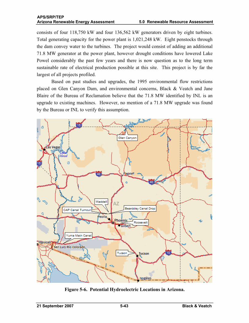
APS/SRP/TEPArizona Renewable Energy Assessment 5.0 Renewable Resource Assessment
21 September 2007 5-43 Black & Veatch
consists of four 118,750 kW and four 136,562 kW generators driven by eight turbines. Total generating capacity for the power plant is 1,021,248 kW. Eight penstocks through the dam convey water to the turbines. The project would consist of adding an additional 71.8 MW generator at the power plant, however drought conditions have lowered Lake Powel considerably the past few years and there is now question as to the long term sustainable rate of electrical production possible at this site. This project is by far the largest of all projects profiled.
Based on past studies and upgrades, the 1995 environmental flow restrictions placed on Glen Canyon Dam, and environmental concerns, Black & Veatch and Jane Blaire of the Bureau of Reclamation believe that the 71.8 MW identified by INL is an upgrade to existing machines. However, no mention of a 71.8 MW upgrade was found by the Bureau or INL to verify this assumption.
Figure 5-6. Potential Hydroelectric Locations in Arizona.
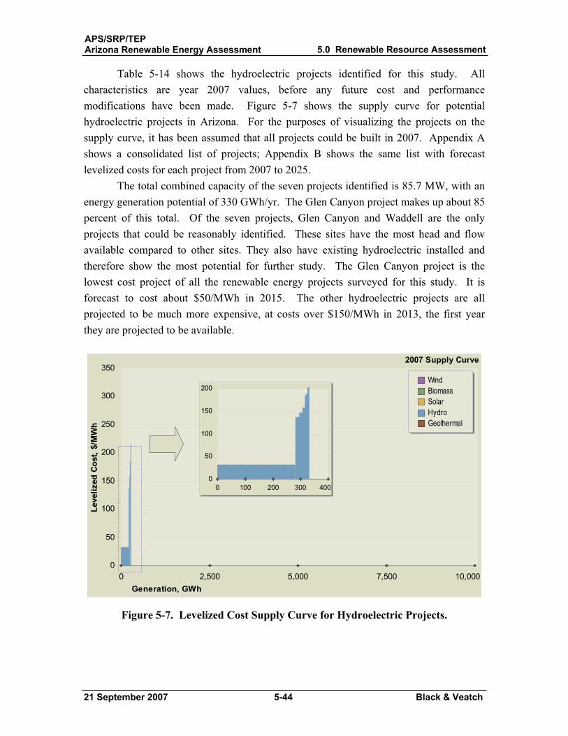
APS/SRP/TEPArizona Renewable Energy Assessment 5.0 Renewable Resource Assessment
21 September 2007 5-44 Black & Veatch
Table 5-14 shows the hydroelectric projects identified for this study. All characteristics are year 2007 values, before any future cost and performance modifications have been made. Figure 5-7 shows the supply curve for potential hydroelectric projects in Arizona. For the purposes of visualizing the projects on the supply curve, it has been assumed that all projects could be built in 2007. Appendix A shows a consolidated list of projects; Appendix B shows the same list with forecast levelized costs for each project from 2007 to 2025.
The total combined capacity of the seven projects identified is 85.7 MW, with an energy generation potential of 330 GWh/yr. The Glen Canyon project makes up about 85 percent of this total. Of the seven projects, Glen Canyon and Waddell are the only projects that could be reasonably identified. These sites have the most head and flow available compared to other sites. They also have existing hydroelectric installed and therefore show the most potential for further study. The Glen Canyon project is the lowest cost project of all the renewable energy projects surveyed for this study. It is forecast to cost about $50/MWh in 2015. The other hydroelectric projects are all projected to be much more expensive, at costs over $150/MWh in 2013, the first year they are projected to be available.
0 2,500 5,000 7,500 10,0000
50
100
150
200
250
300
350
Generation, GWh
Leve
lized
Cos
t, $/
MW
h
WindBiomass SolarHydroGeothermal
2007 Supply Curve
0 100 200 300 4000
50
100
150
200
0 100 200 300 4000
50
100
150
200
Figure 5-7. Levelized Cost Supply Curve for Hydroelectric Projects.
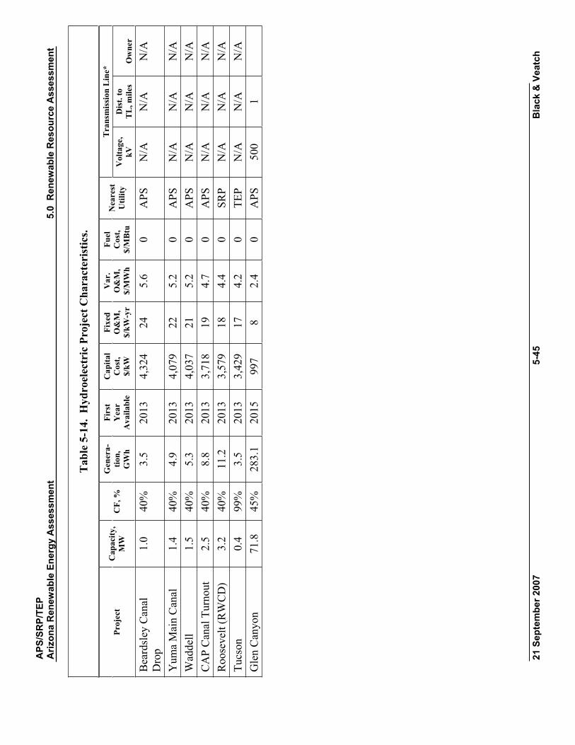
APS
/SR
P/TE
PA
rizon
a R
enew
able
Ene
rgy
Ass
essm
ent
5.0
Ren
ewab
le R
esou
rce
Ass
essm
ent
21 S
epte
mbe
r 200
7 5-
45
Bla
ck &
Vea
tch
Tab
le5-
14.
Hyd
roel
ectr
ic P
roje
ct C
hara
cter
istic
s.
Tra
nsm
issi
on L
ine*
Pr
ojec
t C
apac
ity,
MW
CF,
%
Gen
era-
tion,
GW
h
Firs
tY
ear
Ava
ilabl
e
Cap
ital
Cos
t, $/
kW
Fixe
d O
&M
, $/
kW-y
r
Var
. O
&M
, $/
MW
h
Fuel
C
ost,
$/M
Btu
Nea
rest
U
tility
V
olta
ge,
kVD
ist.
to
TL
, mile
s O
wne
r
Bea
rdsl
ey C
anal
D
rop
1.0
40%
3.
5 20
13
4,32
4 24
5.
6 0
APS
N
/A
N/A
N
/A
Yum
a M
ain
Can
al
1.4
40%
4.
9 20
13
4,07
9 22
5.
2 0
APS
N
/A
N/A
N
/A
Wad
dell
1.5
40%
5.
3 20
13
4,03
7 21
5.
2 0
APS
N
/A
N/A
N
/A
CA
P C
anal
Tur
nout
2.
5 40
%
8.8
2013
3,
718
19
4.7
0 A
PS
N/A
N
/A
N/A
R
oose
velt
(RW
CD
) 3.
2 40
%
11.2
20
13
3,57
9 18
4.
4 0
SRP
N/A
N
/A
N/A
Tu
cson
0.
4 99
%
3.5
2013
3,
429
17
4.2
0 TE
P N
/A
N/A
N
/A
Gle
n C
anyo
n 71
.8
45%
28
3.1
2015
99
7 8
2.4
0 A
PS
500
1

APS/SRP/TEPArizona Renewable Energy Assessment 5.0 Renewable Resource Assessment
21 September 2007 5-46 Black & Veatch
Pumped Storage The following provides and a brief introductory study and summary of two
existing and five proposed pumped storage hydroelectric projects. As part of the preliminary study, pumped storage was not included. For this report existing pumped storage projects were researched using public records available on the internet. Some of the projects looked at had no identifiable locations and limited or no data readily available.
Pumped storage methods are typically used to provide power during peak demand periods. In a pumped storage facility, water is pumped during off-peak demand periods from a reservoir at a lower elevation for storage in a reservoir at a higher elevation. Electricity is then generated during peak demand periods by releasing the pumped water from the higher reservoir and allowing it to flow downhill through the hydraulic turbine(s) connected to generators. During the off-peak pumping cycle, the pumped storage facility is a consumer of electricity which can account for the lower capacity factor. Pumped storage facilities, however, can be economical because they consume low-cost off-peak electricity, but generate high-value on-peak electricity. As with hydroelectric plants, drought conditions can reduce the quantity of on-peak electricity pumped storage facilities can generate.
To date, only a few pumped storage facilities have been built and all are associated with existing dams. Pumped storage can easily be complimented by other renewable resources if available to increase off-peak efficiency. For this study pumped storage was included and was assumed to have a capacity factor of 33 percent.
Table 5-15 lists a summary and descriptions of existing and proposed pumped storage projects in Arizona:
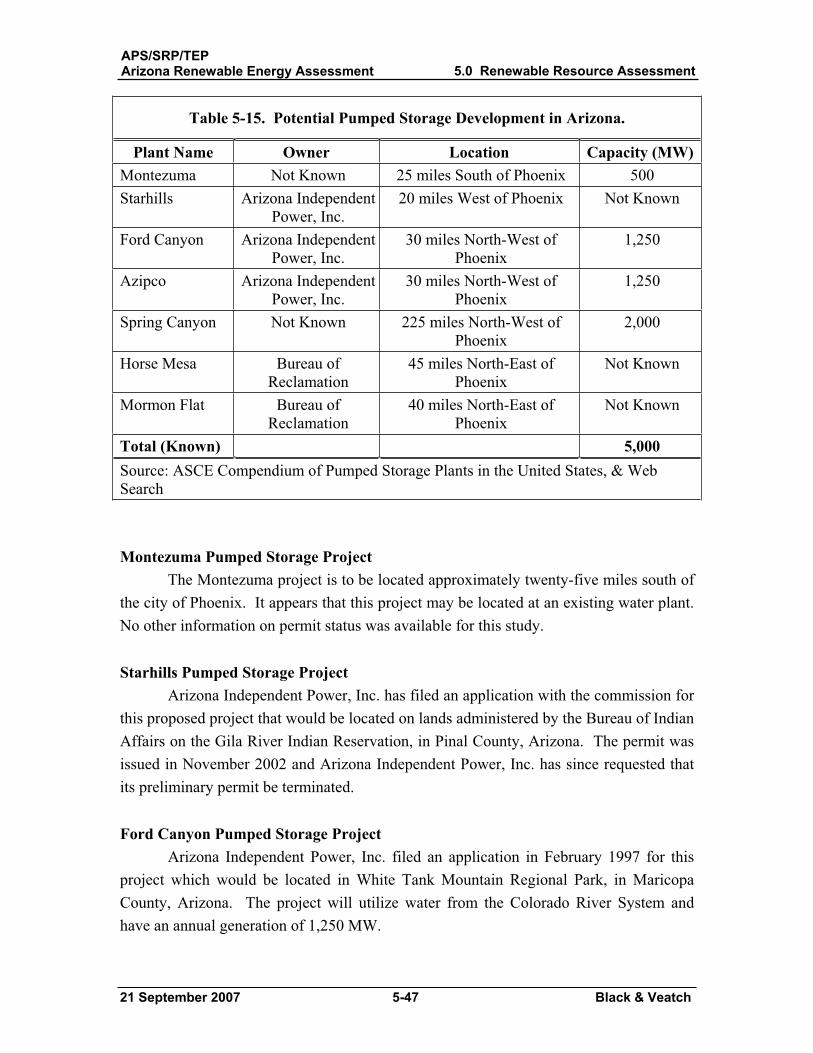
APS/SRP/TEPArizona Renewable Energy Assessment 5.0 Renewable Resource Assessment
21 September 2007 5-47 Black & Veatch
Table 5-15. Potential Pumped Storage Development in Arizona.
Plant Name Owner Location Capacity (MW)Montezuma Not Known 25 miles South of Phoenix 500 Starhills Arizona Independent
Power, Inc. 20 miles West of Phoenix Not Known
Ford Canyon Arizona Independent Power, Inc.
30 miles North-West of Phoenix
1,250
Azipco Arizona Independent Power, Inc.
30 miles North-West of Phoenix
1,250
Spring Canyon Not Known 225 miles North-West of Phoenix
2,000
Horse Mesa Bureau of Reclamation
45 miles North-East of Phoenix
Not Known
Mormon Flat Bureau of Reclamation
40 miles North-East of Phoenix
Not Known
Total (Known) 5,000Source: ASCE Compendium of Pumped Storage Plants in the United States, & Web Search
Montezuma Pumped Storage Project The Montezuma project is to be located approximately twenty-five miles south of
the city of Phoenix. It appears that this project may be located at an existing water plant. No other information on permit status was available for this study.
Starhills Pumped Storage Project Arizona Independent Power, Inc. has filed an application with the commission for
this proposed project that would be located on lands administered by the Bureau of Indian Affairs on the Gila River Indian Reservation, in Pinal County, Arizona. The permit was issued in November 2002 and Arizona Independent Power, Inc. has since requested that its preliminary permit be terminated.
Ford Canyon Pumped Storage Project Arizona Independent Power, Inc. filed an application in February 1997 for this
project which would be located in White Tank Mountain Regional Park, in Maricopa County, Arizona. The project will utilize water from the Colorado River System and have an annual generation of 1,250 MW.
APS/SRP/TEPArizona Renewable Energy Assessment 5.0 Renewable Resource Assessment
21 September 2007 5-48 Black & Veatch
Azipco Pumped Storage Project This project was to be located on the Beardsley Canal, in Maricopa County. The
proposed project would consist of a 350 foot high by 1700 foot long earth and rockfill upper dam. This proposed reservoir would have a surface area of 180 acres and a storage capacity of 13,000 acre-feet and have a normal water surface elevation of 3,000 feet with a proposed 200 foot high by 2600 foot long earth and rockfill lower dam. A proposed reservoir having a surface area of 150 acres and a storage capacity of 14,000 acre-feet with a normal water surface elevation of 1,800 feet would complete the lower portion of this project. The proposed powerhouse would consist of five generating units having a total capacity of 1,250 MW. The original permit was issued in February 2001. Arizona Independent Power, Inc. has requested that its preliminary permit be terminated.
Spring Canyon Pumped Storage Spring Canyon Pumped Storage Project was to have been a 2,000 MW pumped
storage project. This project never went beyond the planning phases. No other information was readily available for this study. This project may have been stopped due to its impacts on the environment. Further study would be necessary to confirm this assumption. No information on permit application could be found, however the application was most likely applied for in the mid to late 1980’s.
Horse Mesa Dam and Reservoir The Horse Mesa Dam and reservoir is located on the Salt River approximately 65
miles northeast of Phoenix. Horse Mesa Dam forms Apache reservoir. One pumped storage hydroelectric unit was added in 1972 and rated at 97,000
kW. The pumped storage unit permits recycling of water for hydroelectric production and keep lake levels relatively constant. The turbine generating units at this dam produce power during periods of peak demands. The turbines are reversed to pump water during off peak periods from the lower reservoir back to the upper reservoir for repeated usage.
Mormon Flat Dam and Reservoir Mormon Flat Dam is a 224-foot high concrete thin-arch structure and is located
on the Salt River 51 miles northeast of Phoenix. Constructed by the Salt River Valley Water Users' Association from 1923-1926, it creates Canyon Lake reservoir.
The pumped storage unit was built in 1971 and is rated at 50,000 kW. The pumped storage unit permits recycling of water for hydroelectric production and keep lake levels relatively constant. The turbine generating units at this dam produce power
APS/SRP/TEPArizona Renewable Energy Assessment 5.0 Renewable Resource Assessment
21 September 2007 5-49 Black & Veatch
during periods of peak demands. The turbines are reversed to pump water during off peak periods from the lower reservoir back to the upper reservoir for repeated usage.
Pumped Storage Summary & Location Map Of the potential capacity identified in Arizona to date, only two pumped storage
facilities have been built and all are associated with existing dams. Pumped storage projects do not appear to be a viable alternative due to it low capacity factor, evaporation, environmental impacts. New pumped storage sites were not identified in this study however, and it is not recommended to consider new pumped storage sites. Due to environmental impacts and permitting issues, it is unlikely that a new pumped storage project would make it past the application process.
Figure 5-8, below identifies the pumped storage projects discussed in this report.
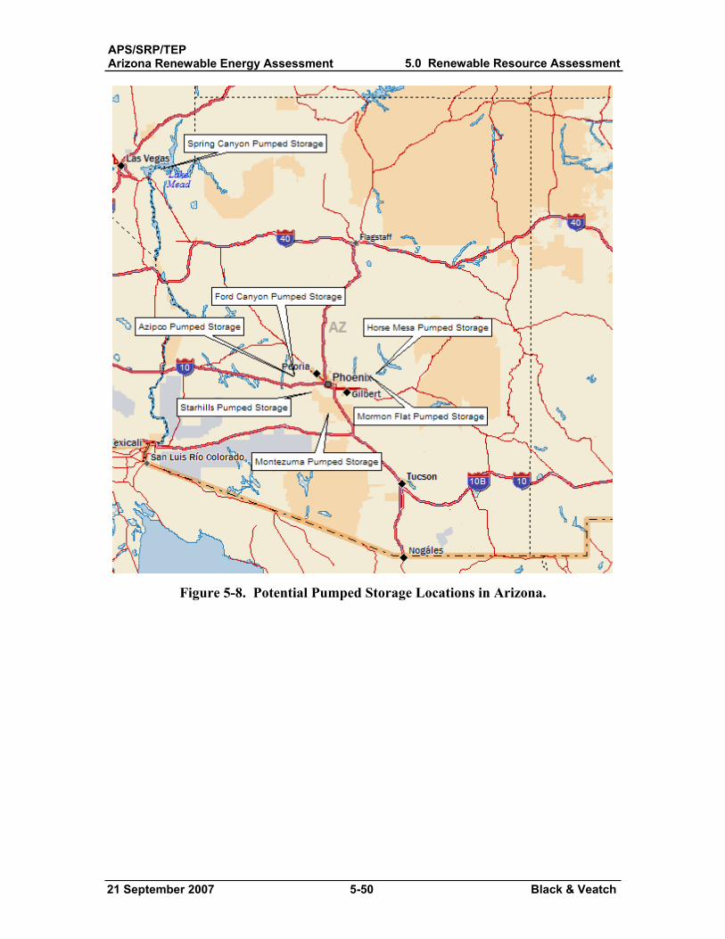
APS/SRP/TEPArizona Renewable Energy Assessment 5.0 Renewable Resource Assessment
21 September 2007 5-50 Black & Veatch
Figure 5-8. Potential Pumped Storage Locations in Arizona.

APS/SRP/TEPArizona Renewable Energy Assessment
5.0 Renewable ResourceAssessment
21 September 2007 5-51 Black & Veatch
5.7 Wind Power Wind power was identified as a promising technology in the first stage of the
analysis. Most of Arizona wind resources are marginal, especially when compared to higher speed wind resources in adjacent states. The economics of wind energy in Arizona vary based on the resource, and the specific attributes of each site will dictate suitable turbine models. This section characterizes the resources suitable for wind technology and those turbines thought to be appropriate for use at the prospective sites.
5.7.1 General Methodology Information was gathered on Arizona’s estimated wind resource, geological
characteristics, transmission infrastructure, environmental and federal land areas in order to identify specific areas conducive to the development of a utility scale wind energy project. Information was collected on current wind development activity in the state. Black & Veatch also spoke with several wind developers, Northern Arizona University, and a member of the Arizona Wind Working group.
An initial list of sites was created based upon the presence of significant land area of at least a class 3 wind resource (greater than 6.3 m/s annual wind speed), which is considered marginal, and specific terrain features that allow a project to be oriented perpendicular with the prevailing wind direction. Each of the sites on this list was then reviewed in light of the following characteristics:
Close proximity to adequate transmission (greater than 69 kV ) Not located within or close to federal or environmentally sensitive areas Constructability
Sites that were not located within 8 to 10 miles of transmission lines with voltages above 69 kV were eliminated from the list. In addition, sites were eliminated in areas with “fatal flaws” due to environmental or other reasons. Of the remaining sites, the next review criteria were based on the overall constructability and suitability of the site.
Each site’s constructability was measured by the ability to both access the wind resource area and construct turbines on it. Sites that had numerous areas of high slope grades and access routes that presented insurmountable equipment delivery issues were eliminated from the list. For those sites deemed to be constructable, site boundaries where created around areas that could likely support the installation of numerous utility scale wind turbines, and had existing access roads or areas where access road construction would likely not be cost prohibitive.
An analysis was then performed for those sites remaining on the list to determine key cost and performance metrics. The following site specific parameters were calculated
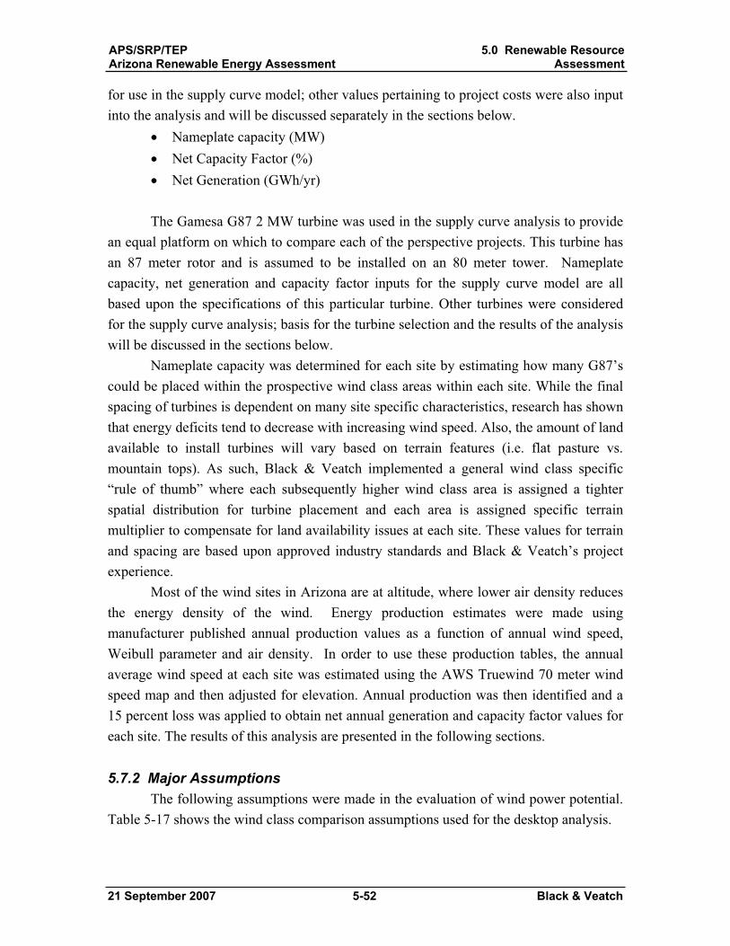
APS/SRP/TEPArizona Renewable Energy Assessment
5.0 Renewable ResourceAssessment
21 September 2007 5-52 Black & Veatch
for use in the supply curve model; other values pertaining to project costs were also input into the analysis and will be discussed separately in the sections below.
Nameplate capacity (MW) Net Capacity Factor (%) Net Generation (GWh/yr)
The Gamesa G87 2 MW turbine was used in the supply curve analysis to provide an equal platform on which to compare each of the perspective projects. This turbine has an 87 meter rotor and is assumed to be installed on an 80 meter tower. Nameplate capacity, net generation and capacity factor inputs for the supply curve model are all based upon the specifications of this particular turbine. Other turbines were considered for the supply curve analysis; basis for the turbine selection and the results of the analysis will be discussed in the sections below.
Nameplate capacity was determined for each site by estimating how many G87’s could be placed within the prospective wind class areas within each site. While the final spacing of turbines is dependent on many site specific characteristics, research has shown that energy deficits tend to decrease with increasing wind speed. Also, the amount of land available to install turbines will vary based on terrain features (i.e. flat pasture vs. mountain tops). As such, Black & Veatch implemented a general wind class specific “rule of thumb” where each subsequently higher wind class area is assigned a tighter spatial distribution for turbine placement and each area is assigned specific terrain multiplier to compensate for land availability issues at each site. These values for terrain and spacing are based upon approved industry standards and Black & Veatch’s project experience.
Most of the wind sites in Arizona are at altitude, where lower air density reduces the energy density of the wind. Energy production estimates were made using manufacturer published annual production values as a function of annual wind speed, Weibull parameter and air density. In order to use these production tables, the annual average wind speed at each site was estimated using the AWS Truewind 70 meter wind speed map and then adjusted for elevation. Annual production was then identified and a 15 percent loss was applied to obtain net annual generation and capacity factor values for each site. The results of this analysis are presented in the following sections.
5.7.2 Major Assumptions The following assumptions were made in the evaluation of wind power potential.
Table 5-17 shows the wind class comparison assumptions used for the desktop analysis.
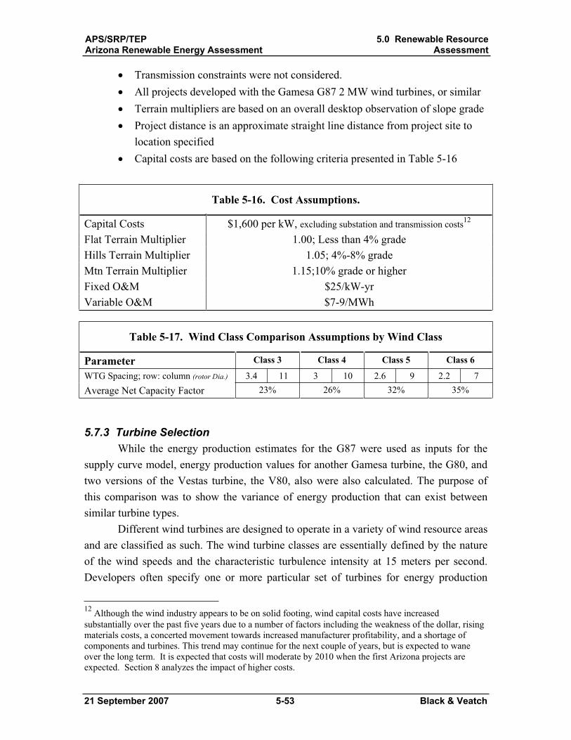
APS/SRP/TEPArizona Renewable Energy Assessment
5.0 Renewable ResourceAssessment
21 September 2007 5-53 Black & Veatch
Transmission constraints were not considered. All projects developed with the Gamesa G87 2 MW wind turbines, or similar Terrain multipliers are based on an overall desktop observation of slope grade Project distance is an approximate straight line distance from project site to location specified Capital costs are based on the following criteria presented in Table 5-16
Table 5-16. Cost Assumptions.
Capital Costs $1,600 per kW, excluding substation and transmission costs12
Flat Terrain Multiplier 1.00; Less than 4% grade Hills Terrain Multiplier 1.05; 4%-8% grade Mtn Terrain Multiplier 1.15;10% grade or higher Fixed O&M $25/kW-yr Variable O&M $7-9/MWh
Table 5-17. Wind Class Comparison Assumptions by Wind Class
Parameter Class 3 Class 4 Class 5 Class 6
WTG Spacing; row: column (rotor Dia.) 3.4 11 3 10 2.6 9 2.2 7 Average Net Capacity Factor 23% 26% 32% 35%
5.7.3 Turbine Selection While the energy production estimates for the G87 were used as inputs for the
supply curve model, energy production values for another Gamesa turbine, the G80, and two versions of the Vestas turbine, the V80, also were also calculated. The purpose of this comparison was to show the variance of energy production that can exist between similar turbine types.
Different wind turbines are designed to operate in a variety of wind resource areas and are classified as such. The wind turbine classes are essentially defined by the nature of the wind speeds and the characteristic turbulence intensity at 15 meters per second. Developers often specify one or more particular set of turbines for energy production
12 Although the wind industry appears to be on solid footing, wind capital costs have increased substantially over the past five years due to a number of factors including the weakness of the dollar, rising materials costs, a concerted movement towards increased manufacturer profitability, and a shortage of components and turbines. This trend may continue for the next couple of years, but is expected to wane over the long term. It is expected that costs will moderate by 2010 when the first Arizona projects are expected. Section 8 analyzes the impact of higher costs.
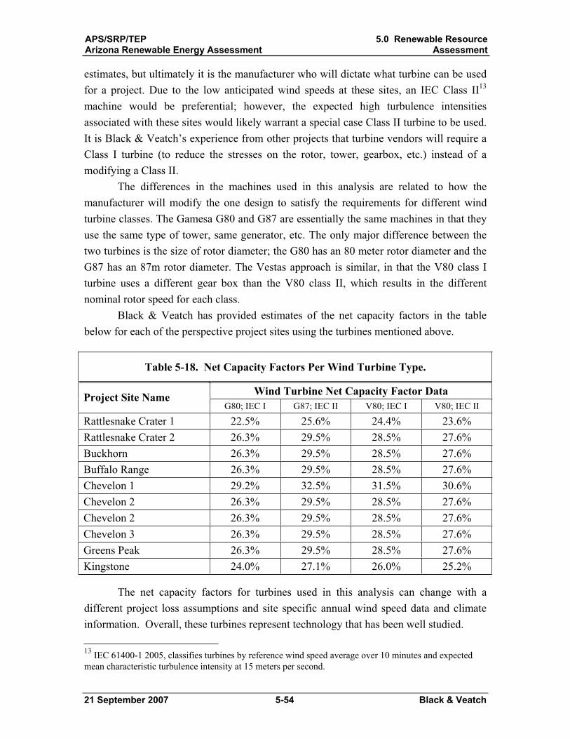
APS/SRP/TEPArizona Renewable Energy Assessment
5.0 Renewable ResourceAssessment
21 September 2007 5-54 Black & Veatch
estimates, but ultimately it is the manufacturer who will dictate what turbine can be used for a project. Due to the low anticipated wind speeds at these sites, an IEC Class II13
machine would be preferential; however, the expected high turbulence intensities associated with these sites would likely warrant a special case Class II turbine to be used. It is Black & Veatch’s experience from other projects that turbine vendors will require a Class I turbine (to reduce the stresses on the rotor, tower, gearbox, etc.) instead of a modifying a Class II.
The differences in the machines used in this analysis are related to how the manufacturer will modify the one design to satisfy the requirements for different wind turbine classes. The Gamesa G80 and G87 are essentially the same machines in that they use the same type of tower, same generator, etc. The only major difference between the two turbines is the size of rotor diameter; the G80 has an 80 meter rotor diameter and the G87 has an 87m rotor diameter. The Vestas approach is similar, in that the V80 class I turbine uses a different gear box than the V80 class II, which results in the different nominal rotor speed for each class.
Black & Veatch has provided estimates of the net capacity factors in the table below for each of the perspective project sites using the turbines mentioned above.
Table 5-18. Net Capacity Factors Per Wind Turbine Type.
Wind Turbine Net Capacity Factor Data Project Site Name G80; IEC I G87; IEC II V80; IEC I V80; IEC II
Rattlesnake Crater 1 22.5% 25.6% 24.4% 23.6% Rattlesnake Crater 2 26.3% 29.5% 28.5% 27.6% Buckhorn 26.3% 29.5% 28.5% 27.6% Buffalo Range 26.3% 29.5% 28.5% 27.6% Chevelon 1 29.2% 32.5% 31.5% 30.6% Chevelon 2 26.3% 29.5% 28.5% 27.6% Chevelon 2 26.3% 29.5% 28.5% 27.6% Chevelon 3 26.3% 29.5% 28.5% 27.6% Greens Peak 26.3% 29.5% 28.5% 27.6% Kingstone 24.0% 27.1% 26.0% 25.2%
The net capacity factors for turbines used in this analysis can change with a different project loss assumptions and site specific annual wind speed data and climate information. Overall, these turbines represent technology that has been well studied. 13 IEC 61400-1 2005, classifies turbines by reference wind speed average over 10 minutes and expected mean characteristic turbulence intensity at 15 meters per second.

APS/SRP/TEPArizona Renewable Energy Assessment
5.0 Renewable ResourceAssessment
21 September 2007 5-55 Black & Veatch
5.7.4 Future Cost and Performance Projections Wind technology has improved measurable over the last few years. As part of
work performed for the American Wind Energy Association, Black & Veatch analyzed monthly capacity factor data from over 5,000 MW of wind plants installed in the US Midwest for the years 2000 through 2005. The Midwest was chosen to ensure all the plants were in a similar wind regime. Capacity factors have shown enormous improvement, averaging 15 percent improvement every two years. This improvement is due to improved availability, increased hub heights and rotor diameters, as well as better siting. Average hub heights went from roughly 60 meters in 2000-2001 to 85 meters in 2005. Rotor diameters increased from 47 meters to 80 or 90 meters, doubling swept area.
Black & Veatch believes this improvement will continue, although at a slower pace. Capacity factors are forecast to increase another 20 percent from 2005 to 2030, based on higher hub heights, larger rotors, and advanced power electronics.
5.7.5 Data Sources Data sources used in this analysis included:
AWS TrueWind, Arizona Wind Maps Elliott, D.L, 1991, “Status of Wake and Array Loss Research”, Pacific Northwest Laboratory, Richland, Washington “The Arizona Meteorological Network”, available at: http://ag.arizona.edu/AZMET/.html, accessed: March, 2007 “Geospatial Data and Metadata Statewide Coverages for Arizona BLM”, available at: http://www.blm.gov/az/gis/files.htm, accessed: March, 2007 Northern Arizona University, available at: http://wind.nau.edu/, accessed: March, 2007 IEC 61400-1 2005, Wind Turbines – Part 1: Design requirement
5.7.6 Projects Identified At the conclusion of the review, ten projects at six sites totaling 991 MW of wind
energy remained from the original list. Black & Veatch estimates that the total production of these projects will annually yield 2,551 GWh, with an average project net capacity factor of 28.9 percent. The characteristics of these individual projects are provided in Table 5-19. Figure 5-9 shows the general locations of each of the identified project areas overlain on a wind speed map for Arizona. The following sections contain descriptions of each project. Each section contains a map which has the local wind speed map overlain on the site topography. Transmission lines are also indicated. Military training zones may impact the total developable amounts of wind generation and should be

APS/SRP/TEPArizona Renewable Energy Assessment
5.0 Renewable ResourceAssessment
21 September 2007 5-56 Black & Veatch
reviewed in detail before project development. Additionally, the Arizona Fish and Game Department has recommended that a three year bird and bat study be performed prior to commencing a wind project in Arizona. Finally, while it is possible that other wind sites could be developed in Arizona, these sites are either further from transmission, have environmental restrictions, are in difficult to construct areas, or have weaker wind resources.
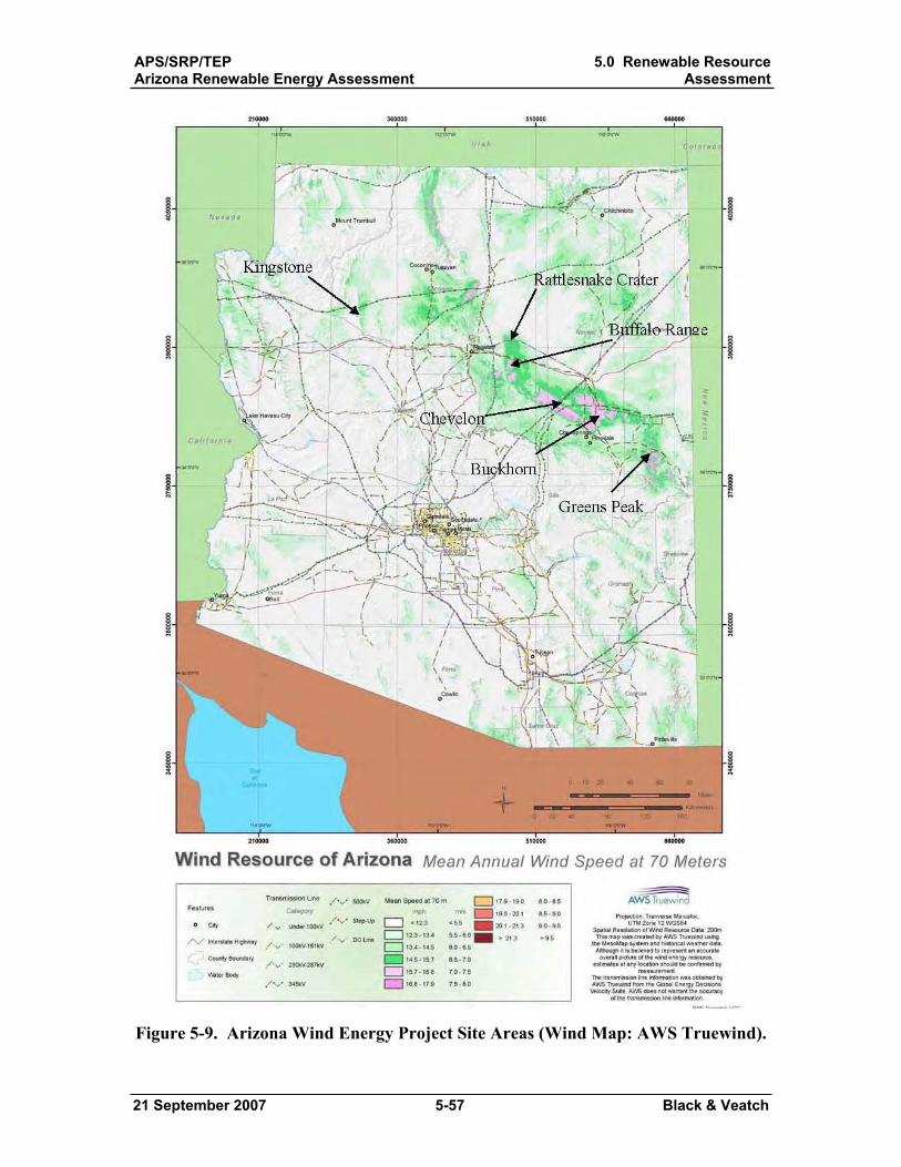
APS/SRP/TEPArizona Renewable Energy Assessment
5.0 Renewable ResourceAssessment
21 September 2007 5-57 Black & Veatch
Figure 5-9. Arizona Wind Energy Project Site Areas (Wind Map: AWS Truewind).
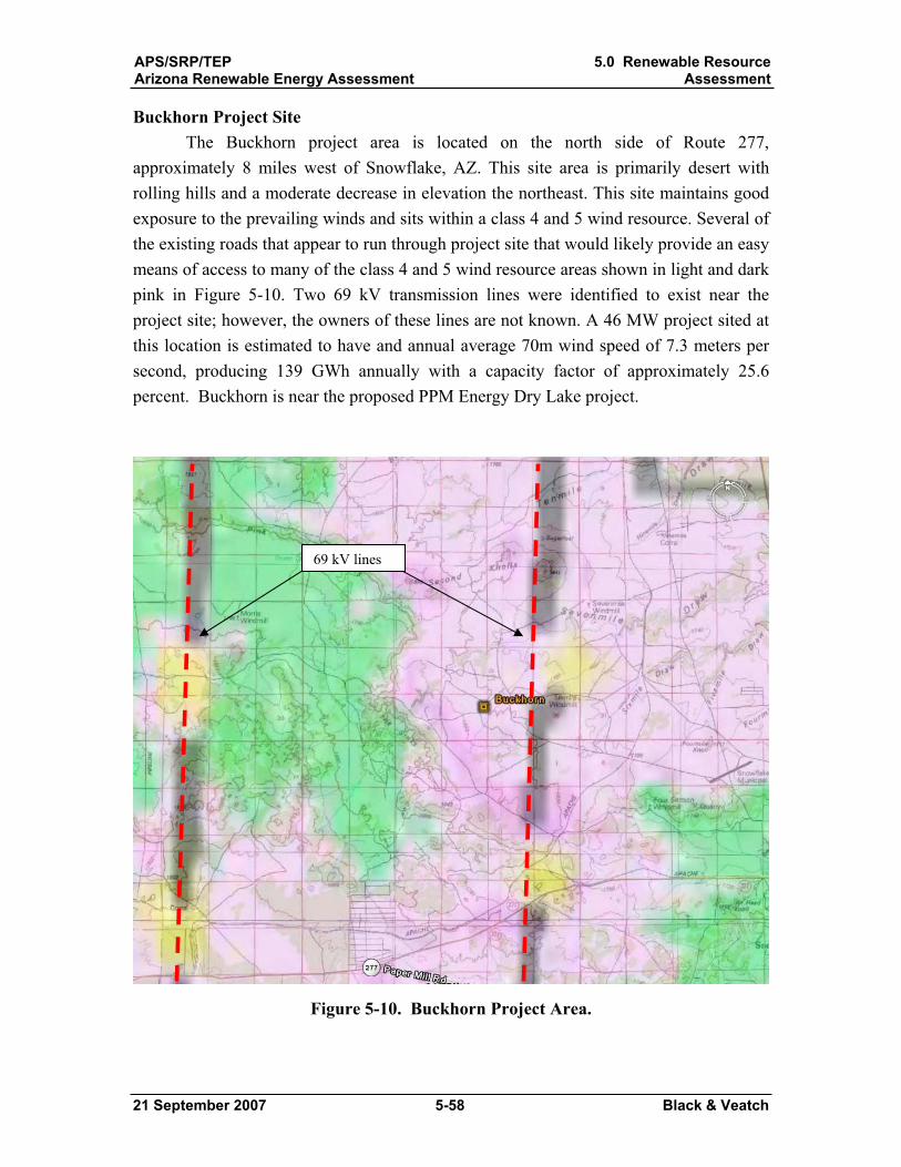
APS/SRP/TEPArizona Renewable Energy Assessment
5.0 Renewable ResourceAssessment
21 September 2007 5-58 Black & Veatch
Buckhorn Project Site The Buckhorn project area is located on the north side of Route 277,
approximately 8 miles west of Snowflake, AZ. This site area is primarily desert with rolling hills and a moderate decrease in elevation the northeast. This site maintains good exposure to the prevailing winds and sits within a class 4 and 5 wind resource. Several of the existing roads that appear to run through project site that would likely provide an easy means of access to many of the class 4 and 5 wind resource areas shown in light and dark pink in Figure 5-10. Two 69 kV transmission lines were identified to exist near the project site; however, the owners of these lines are not known. A 46 MW project sited at this location is estimated to have and annual average 70m wind speed of 7.3 meters per second, producing 139 GWh annually with a capacity factor of approximately 25.6 percent. Buckhorn is near the proposed PPM Energy Dry Lake project.
Figure 5-10. Buckhorn Project Area.
69 kV lines
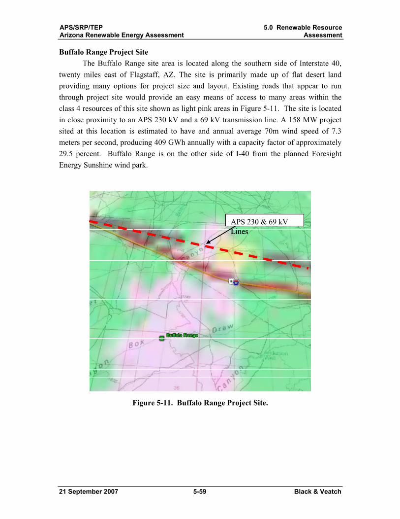
APS/SRP/TEPArizona Renewable Energy Assessment
5.0 Renewable ResourceAssessment
21 September 2007 5-59 Black & Veatch
Buffalo Range Project Site The Buffalo Range site area is located along the southern side of Interstate 40,
twenty miles east of Flagstaff, AZ. The site is primarily made up of flat desert land providing many options for project size and layout. Existing roads that appear to run through project site would provide an easy means of access to many areas within the class 4 resources of this site shown as light pink areas in Figure 5-11. The site is located in close proximity to an APS 230 kV and a 69 kV transmission line. A 158 MW project sited at this location is estimated to have and annual average 70m wind speed of 7.3 meters per second, producing 409 GWh annually with a capacity factor of approximately 29.5 percent. Buffalo Range is on the other side of I-40 from the planned Foresight Energy Sunshine wind park.
APS 230 & 69 kV LinesAPS 230 & 69 kV LinesAPS 230 & 69 kV Lines
Figure 5-11. Buffalo Range Project Site.
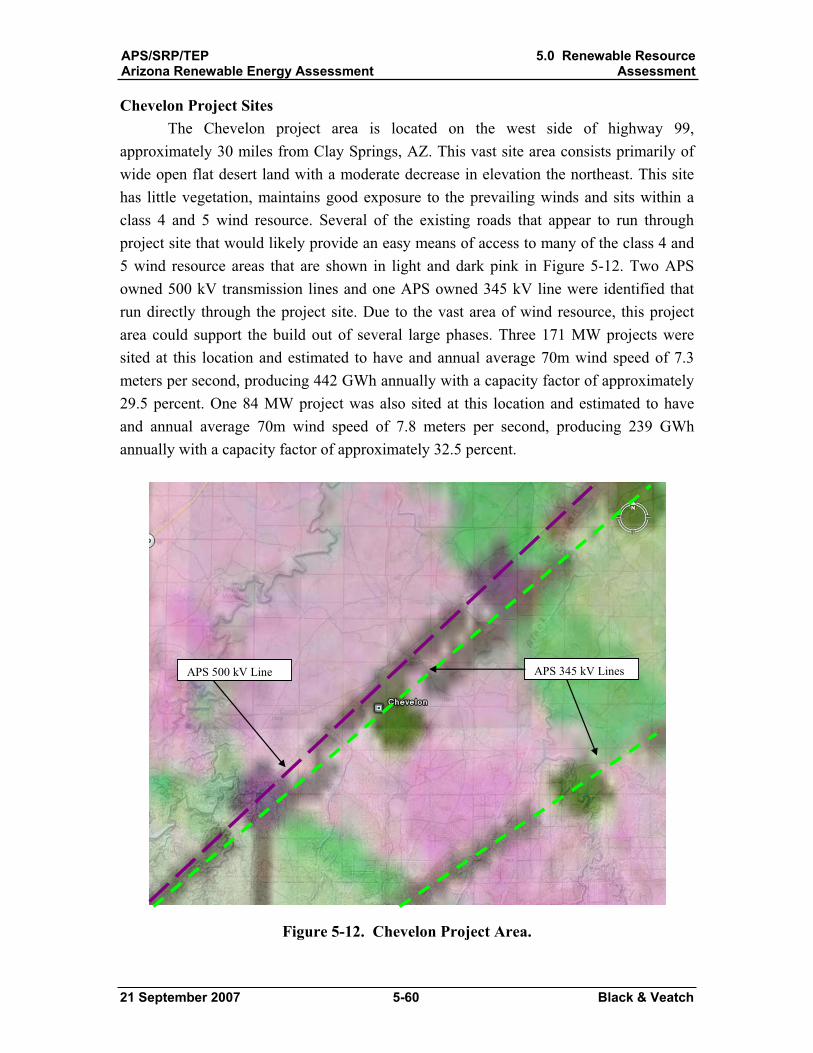
APS/SRP/TEPArizona Renewable Energy Assessment
5.0 Renewable ResourceAssessment
21 September 2007 5-60 Black & Veatch
Chevelon Project Sites The Chevelon project area is located on the west side of highway 99,
approximately 30 miles from Clay Springs, AZ. This vast site area consists primarily of wide open flat desert land with a moderate decrease in elevation the northeast. This site has little vegetation, maintains good exposure to the prevailing winds and sits within a class 4 and 5 wind resource. Several of the existing roads that appear to run through project site that would likely provide an easy means of access to many of the class 4 and 5 wind resource areas that are shown in light and dark pink in Figure 5-12. Two APS owned 500 kV transmission lines and one APS owned 345 kV line were identified that run directly through the project site. Due to the vast area of wind resource, this project area could support the build out of several large phases. Three 171 MW projects were sited at this location and estimated to have and annual average 70m wind speed of 7.3 meters per second, producing 442 GWh annually with a capacity factor of approximately 29.5 percent. One 84 MW project was also sited at this location and estimated to have and annual average 70m wind speed of 7.8 meters per second, producing 239 GWh annually with a capacity factor of approximately 32.5 percent.
APS 345 kV LinesAPS 500 kV Line
Figure 5-12. Chevelon Project Area.

APS/SRP/TEPArizona Renewable Energy Assessment
5.0 Renewable ResourceAssessment
21 September 2007 5-61 Black & Veatch
Greens Peak Project Site The Greens Peak project area is located on the north side of Highway 260,
approximately 14 miles west of Springerville, AZ. While this site area is primarily desert with rolling hills, the landscape is covered with thick vegetation and a few areas of complex terrain features. Exposure of this site to prevailing winds appears to be somewhat restricted to specific areas; however, wind resource maps indicate that strong class 4 and 5 wind resources present in this area. Several of the existing roads that appear to run through project site that would likely provide an easy means of access to many of the wind resource areas shown in light and dark pink in Figure 5-13. Several Navopache Electric Cooperative owned 69 kV transmission lines were identified to exist near the project site. A 31 MW project sited at this location is estimated to have and annual average 70m wind speed of 7.6 meters per second, producing 79 GWh annually with a capacity factor of approximately 29.5 percent.
69 kV lines69 kV lines
Figure 5-13. Greens Peak Project Area.
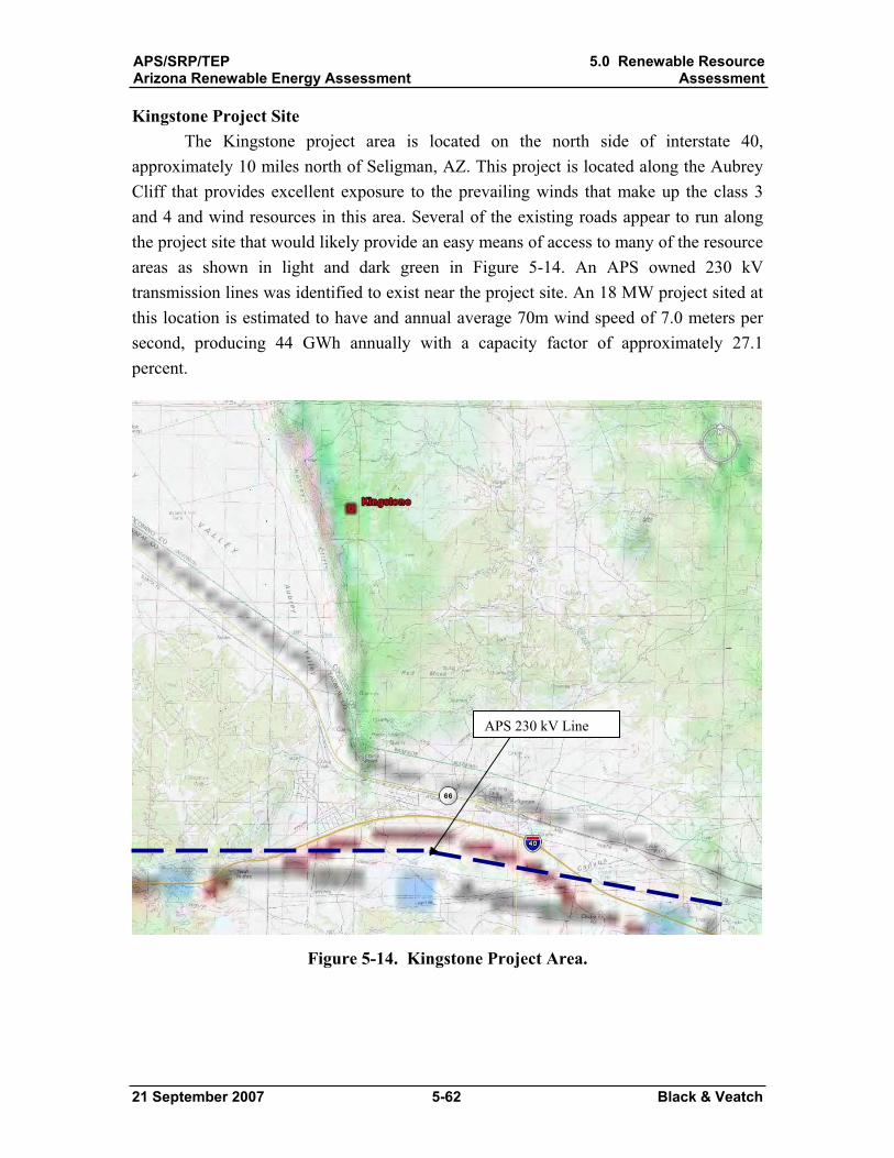
APS/SRP/TEPArizona Renewable Energy Assessment
5.0 Renewable ResourceAssessment
21 September 2007 5-62 Black & Veatch
Kingstone Project Site The Kingstone project area is located on the north side of interstate 40,
approximately 10 miles north of Seligman, AZ. This project is located along the Aubrey Cliff that provides excellent exposure to the prevailing winds that make up the class 3 and 4 and wind resources in this area. Several of the existing roads appear to run along the project site that would likely provide an easy means of access to many of the resource areas as shown in light and dark green in Figure 5-14. An APS owned 230 kV transmission lines was identified to exist near the project site. An 18 MW project sited at this location is estimated to have and annual average 70m wind speed of 7.0 meters per second, producing 44 GWh annually with a capacity factor of approximately 27.1 percent.
Figure 5-14. Kingstone Project Area.
APS 230 kV Line
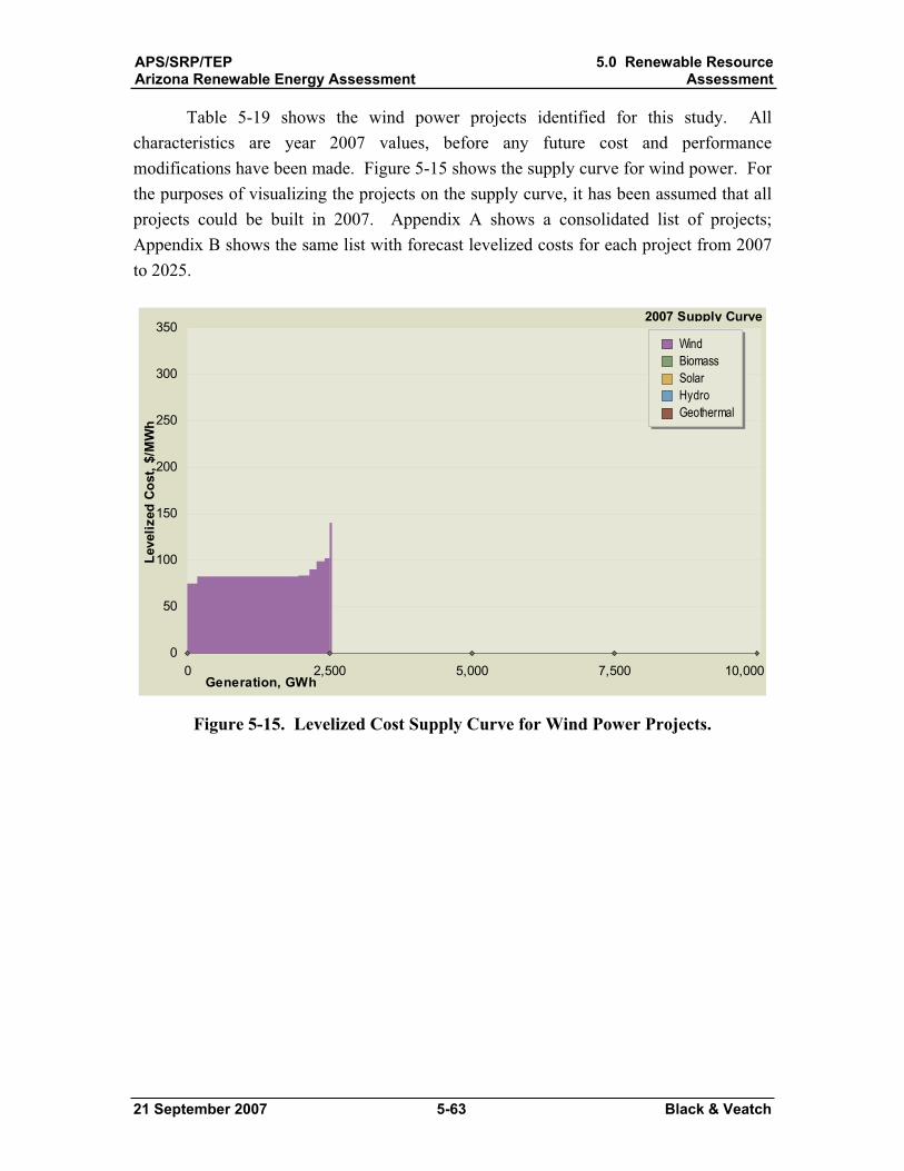
APS/SRP/TEPArizona Renewable Energy Assessment
5.0 Renewable ResourceAssessment
21 September 2007 5-63 Black & Veatch
Table 5-19 shows the wind power projects identified for this study. All characteristics are year 2007 values, before any future cost and performance modifications have been made. Figure 5-15 shows the supply curve for wind power. For the purposes of visualizing the projects on the supply curve, it has been assumed that all projects could be built in 2007. Appendix A shows a consolidated list of projects; Appendix B shows the same list with forecast levelized costs for each project from 2007 to 2025.
0 2,500 5,000 7,500 10,0000
50
100
150
200
250
300
350
Generation, GWh
Leve
lized
Cos
t, $/
MW
h
WindBiomass SolarHydroGeothermal
2007 Supply Curve
Figure 5-15. Levelized Cost Supply Curve for Wind Power Projects.
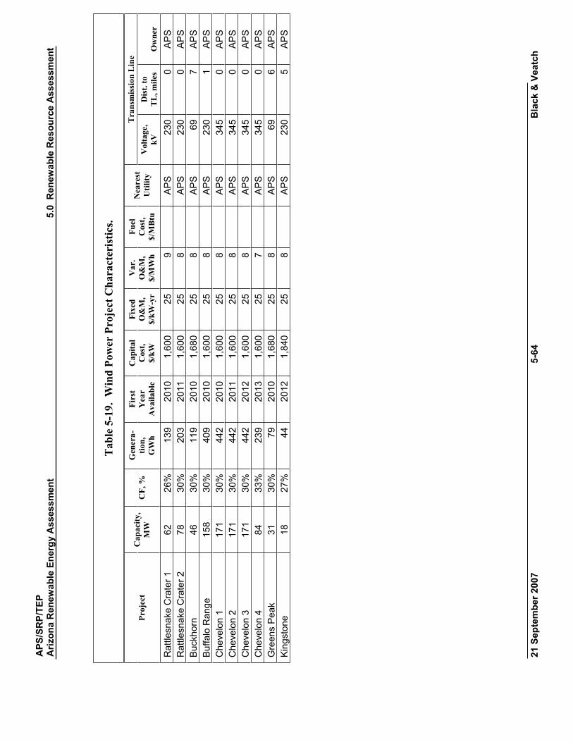
APS
/SR
P/TE
PA
rizon
a R
enew
able
Ene
rgy
Ass
essm
ent
5.0
Ren
ewab
le R
esou
rce
Ass
essm
ent
21 S
epte
mbe
r 200
7 5-
64
Bla
ck &
Vea
tch
Tab
le5-
19.
Win
d Po
wer
Pro
ject
Cha
ract
eris
tics.
Tra
nsm
issi
on L
ine
Proj
ect
Cap
acity
, M
WC
F, %
G
ener
a-tio
n,G
Wh
Firs
tY
ear
Ava
ilabl
e
Cap
ital
Cos
t, $/
kW
Fixe
d O
&M
, $/
kW-y
r
Var
. O
&M
, $/
MW
h
Fuel
C
ost,
$/M
Btu
Nea
rest
U
tility
V
olta
ge,
kVD
ist.
to
TL
, mile
s O
wne
r
Rat
tlesn
ake
Cra
ter 1
62
26
%13
920
101,
600
25
9A
PS
23
00
AP
S
Rat
tlesn
ake
Cra
ter 2
78
30
%20
320
111,
600
25
8A
PS
23
00
AP
S
Buc
khor
n 46
30
%11
920
101,
680
25
8A
PS
69
7A
PS
B
uffa
lo R
ange
15
8 30
%40
920
101,
600
25
8A
PS
23
01
AP
S
Che
velo
n 1
171
30%
442
2010
1,60
025
8
AP
S
345
0A
PS
C
heve
lon
2 17
1 30
%44
220
111,
600
25
8A
PS
34
50
AP
S
Che
velo
n 3
171
30%
442
2012
1,60
025
8
AP
S
345
0A
PS
C
heve
lon
4 84
33
%23
920
131,
600
25
7A
PS
34
50
AP
S
Gre
ens
Pea
k 31
30
%79
2010
1,68
025
8
AP
S
696
AP
S
Kin
gsto
ne
18
27%
4420
121,
840
25
8A
PS
23
05
AP
S
APS/SRP/TEPArizona Renewable Energy Assessment
5.0 Renewable ResourceAssessment
21 September 2007 5-65 Black & Veatch
5.8 Geothermal Geothermal was identified as a relatively unquantified, but potentially promising
resource in the first phase of this study. This section explores two potential projects in more detail.
5.8.1 General Methodology In Arizona, the geothermal resource is not as well explored and characterized as
in some areas of the Southwestern United States. Electric power production from geothermal is undemonstrated in Arizona. Because of the limited work done to this point to identify specific developable geothermal resources in the state, projects are based on the two areas where there has been some focus on understanding the resource potential.
Without a known location that would support a flash steam geothermal facility, binary cycle type plants have been characterized.
5.8.2 Major Assumptions Because projects are still in their early exploratory state, there is not enough data
available to accurately characterize the geothermal projects with a high degree of precision. Even identifying the potential project size is still speculative. For this reason, generic project assumptions (similar to those presented in Section 4) were adjusted for economies of scale and then applied to the two projects identified.
The following assumptions were made in the evaluation of geothermal potential. Two sites, Gillard Hot Springs and Clifton 15 and 20 MW power plants Binary cycle plant type Construction time of 3.5 years Available for operation in 2013 and 2014 Capacity factor of 70 percent, which is typical for dry-cooled binary resources (the most likely type to be developed in Arizona)
At best, these assumptions identify “place-holder” projects that must be further defined as more information about the true potential of each site is discovered.
5.8.3 Future Cost and Performance Projections The geothermal technologies of flash steam and binary cycle are largely mature
technologies. No changes in their future cost or performance were assumed. “Enhanced Geothermal Systems” described below, are new techniques that may bring more
APS/SRP/TEPArizona Renewable Energy Assessment
5.0 Renewable ResourceAssessment
21 September 2007 5-66 Black & Veatch
geothermal development to Arizona, not because of lower costs or higher efficiencies, but because they may make new geothermal resource areas available for production.
Although the focus for most geothermal projects to date has been conventional hydrothermal resources, there is considerable potential in Arizona for the so-called “Enhanced Geothermal Systems” or “Hot Dry Rock” type of projects. Such projects are developed in areas with high underground temperatures but insufficient permeability to support commercial flow rates. In such projects, the reservoir rock is stimulated by hydraulic and/or chemical methods, creating a large network of fine fractures, thus forming an underground heat exchanger. Fluid is injected at one location and produced at another, having passed through the fracture network, gaining heat on the way. These non-conventional resources are experimental and strategic at this point, but many projects are underway in the US, Europe and Australia to determine the most effective methods of stimulation and heat recovery. The project at Soultz-sous-Forêts in France is likely to be the first to produce power from EGS/HDR resources, with one of the Australian projects likely to be the next. This type of development is probably 10 years or more from being commercial; more experience in the development and operational aspects of EGS/HDR resources is needed, and cost reductions need to enable this technology to be considered commercial. EGS/HDR resources were not explicitly modeled in this study. However, there appears to be sufficient promise that development of the technology should be closely monitored.
5.8.4 Data Sources Data sources used in this analysis included:
NOAA (National Oceanic and Atmospheric Administration, 1982. Geothermal Resources of Arizona. Oversized map with text and tables. INL (Idaho National Engineering and Environmental Laboratory), 2003.Arizona Geothermal Resources. One-page map. Publication No. INL/MIS-2002-1616 Rev.1. Witcher, James C., 1995. Geothermal Resource Data Base: Arizona.”Southwest Technology Development Institute, New Mexico State University. David Brown and Associates, 2006. GRED III Final Report, Clifton Hot Springs Geothermal Project, Greenlee County, Arizona. Report on worked funded by US Department of Energy, DE-FC36-04GO14346. Morgan, P., W. Duffield., J. Sass and T. Felger, 2003. Searthing for an electrical-grade geothermal resource in northern Arizona to help Geopower the West. Transactions, Geothermal Resources Council, Vol. 27.
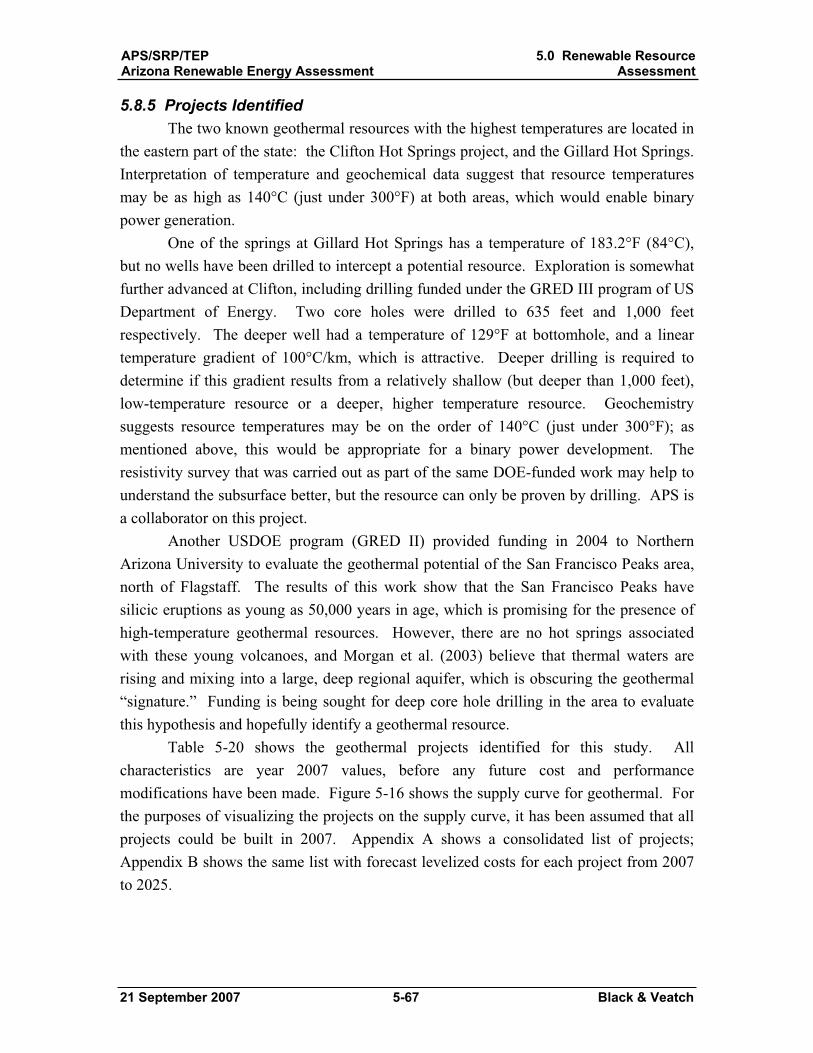
APS/SRP/TEPArizona Renewable Energy Assessment
5.0 Renewable ResourceAssessment
21 September 2007 5-67 Black & Veatch
5.8.5 Projects Identified The two known geothermal resources with the highest temperatures are located in
the eastern part of the state: the Clifton Hot Springs project, and the Gillard Hot Springs. Interpretation of temperature and geochemical data suggest that resource temperatures may be as high as 140°C (just under 300°F) at both areas, which would enable binary power generation.
One of the springs at Gillard Hot Springs has a temperature of 183.2°F (84°C), but no wells have been drilled to intercept a potential resource. Exploration is somewhat further advanced at Clifton, including drilling funded under the GRED III program of US Department of Energy. Two core holes were drilled to 635 feet and 1,000 feet respectively. The deeper well had a temperature of 129°F at bottomhole, and a linear temperature gradient of 100°C/km, which is attractive. Deeper drilling is required to determine if this gradient results from a relatively shallow (but deeper than 1,000 feet), low-temperature resource or a deeper, higher temperature resource. Geochemistry suggests resource temperatures may be on the order of 140°C (just under 300°F); as mentioned above, this would be appropriate for a binary power development. The resistivity survey that was carried out as part of the same DOE-funded work may help to understand the subsurface better, but the resource can only be proven by drilling. APS is a collaborator on this project.
Another USDOE program (GRED II) provided funding in 2004 to Northern Arizona University to evaluate the geothermal potential of the San Francisco Peaks area, north of Flagstaff. The results of this work show that the San Francisco Peaks have silicic eruptions as young as 50,000 years in age, which is promising for the presence of high-temperature geothermal resources. However, there are no hot springs associated with these young volcanoes, and Morgan et al. (2003) believe that thermal waters are rising and mixing into a large, deep regional aquifer, which is obscuring the geothermal “signature.” Funding is being sought for deep core hole drilling in the area to evaluate this hypothesis and hopefully identify a geothermal resource.
Table 5-20 shows the geothermal projects identified for this study. All characteristics are year 2007 values, before any future cost and performance modifications have been made. Figure 5-16 shows the supply curve for geothermal. For the purposes of visualizing the projects on the supply curve, it has been assumed that all projects could be built in 2007. Appendix A shows a consolidated list of projects; Appendix B shows the same list with forecast levelized costs for each project from 2007 to 2025.

APS
/SR
P/TE
PA
rizon
a R
enew
able
Ene
rgy
Ass
essm
ent
5.0
Ren
ewab
le R
esou
rce
Ass
essm
ent
21 S
epte
mbe
r 200
7 5-
68
Bla
ck &
Vea
tch
Tab
le5-
20.
Geo
ther
mal
Pro
ject
Cha
ract
eris
tics.
Tra
nsm
issi
on L
ine
Proj
ect
Cap
acity
, M
WC
F, %
G
ener
a-tio
n,G
Wh
Firs
tY
ear
Ava
ilabl
e
Cap
ital
Cos
t, $/
kW
Fixe
d O
&M
, $/
kW-y
r
Var
. O
&M
, $/
MW
h
Fuel
C
ost,
$/M
Btu
Nea
rest
U
tility
V
olta
ge, k
VD
ist.
to T
L,
mile
s O
wne
r C
lifto
n 20
.0
70%
12
3 20
13
4,00
0
30
0A
PS
35
10
Gill
ard
15.0
70
%
92
2014
4,
500
30
0
APS
35
10
N
ote:
Tra
nsm
issi
on L
ine
volta
ge a
nd D
ista
nce
to tr
ansm
issi
on li
ne is
unk
now
n.
Fixe
d O
&M
cos
ts a
re in
clud
ed in
the
capi
tal c
ost a
nd v
aria
ble
O&
M c
ost n
umbe
rs.
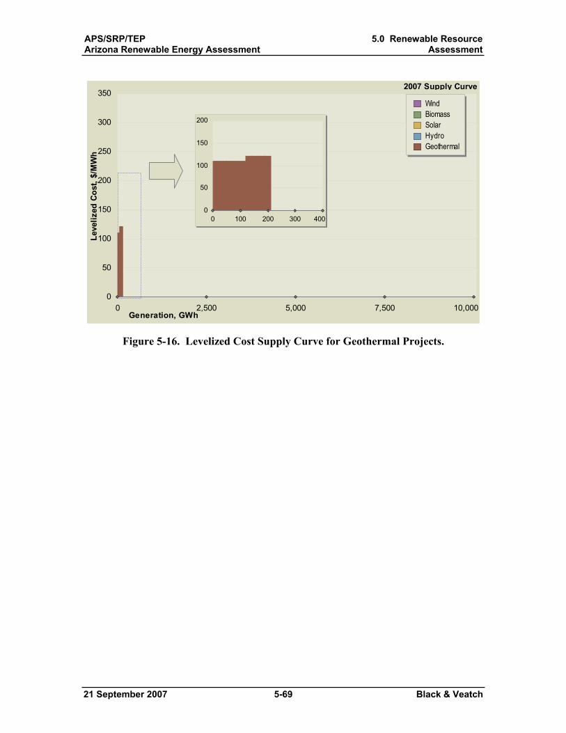
APS/SRP/TEPArizona Renewable Energy Assessment
5.0 Renewable ResourceAssessment
21 September 2007 5-69 Black & Veatch
0 2,500 5,000 7,500 10,0000
50
100
150
200
250
300
350
Generation, GWh
Leve
lized
Cos
t, $/
MW
hWindBiomass SolarHydroGeothermal
2007 Supply Curve
0 100 200 300 4000
50
100
150
200
0 100 200 300 4000
50
100
150
200
Figure 5-16. Levelized Cost Supply Curve for Geothermal Projects.
APS/SRP/TEPArizona Renewable Energy Assessment
6.0 Renewable Energy FinancialIncentives
21 September 2007 6-1 Black & Veatch
6.0 Renewable Energy Financial Incentives
A number of financial incentives are available for the installation and operation of renewable energy technologies. These incentives can substantially influence profitability and can make the difference between a non-viable and a viable project. The following discussion provides a brief list of existing and proposed incentives that are available to new renewable energy facilities. Although many of these incentives are designed as tax credits, it may still be possible for non-taxable entities (or others with limited tax appetite) to benefit from the incentives by establishing facility ownership through a third-party taxable entity or other project structures. It should be noted that the intent of this section is to provide general information on available incentives; Black & Veatch cannot provide tax advice concerning the implications of the specific incentive programs.
6.1 Tax Related Incentives The predominant incentive offered by the federal government for renewable
energy has been through the US tax code in the form of tax deductions, tax credits, or accelerated depreciation. An advantage of this form of incentive is that it is defined in the tax code and is not subject to annual congressional appropriations or other limited budget pools (such as grants and loans). Tax related incentives include:
Section 45 Production Tax Credit (PTC) Section 48 Investment Tax Credit (ITC) Accelerated depreciation
The ability to utilize tax credits is limited not only by specific legal considerations, but also by practical considerations. It can be difficult to line up the risks and benefits of a specific transaction with the appropriate participants and their tax status.
Government-owned utilities and other tax-exempt entities are not able to directly take advantage of these tax incentives. Tax-exempt entities, however, do enjoy a number of other benefits when financing and operating capital investments. The most obvious benefit is freedom from federal and state income tax liability. Depending on project location and local laws, payment of property taxes may also be reduced or eliminated. These entities are also able to issue tax-exempt debt, which carries considerably lower interest rates than comparable corporate debt.
The Section 45 PTC is available to private entities subject to taxation for the production of electricity from various renewable energy technologies. The Energy Policy Act of 2005 expanded and extended the PTC through 2007. The PTC was further extended in late 2006 until the end of 2008. For most technologies, the facility must be in service by December 31, 2008. The income tax credit amounts to 1.5 cents/kWh
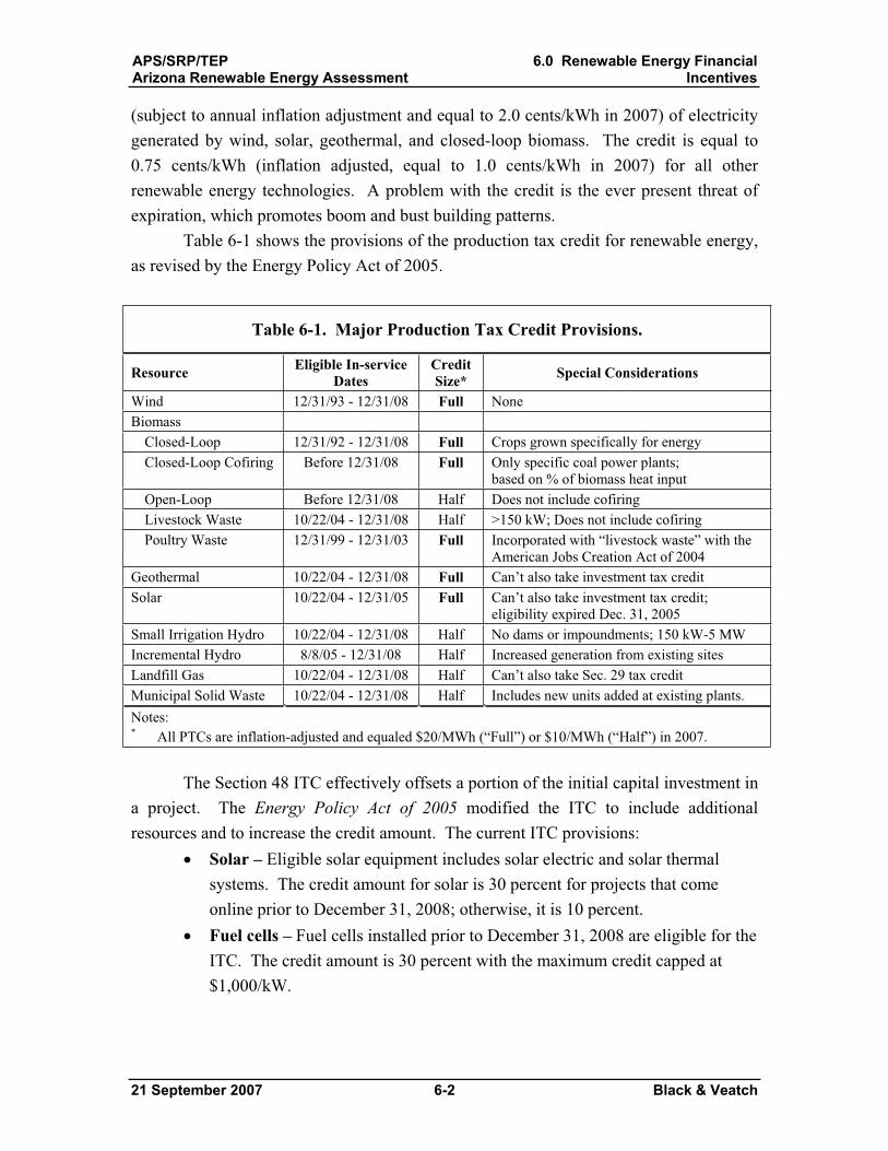
APS/SRP/TEPArizona Renewable Energy Assessment
6.0 Renewable Energy FinancialIncentives
21 September 2007 6-2 Black & Veatch
(subject to annual inflation adjustment and equal to 2.0 cents/kWh in 2007) of electricity generated by wind, solar, geothermal, and closed-loop biomass. The credit is equal to 0.75 cents/kWh (inflation adjusted, equal to 1.0 cents/kWh in 2007) for all other renewable energy technologies. A problem with the credit is the ever present threat of expiration, which promotes boom and bust building patterns.
Table 6-1 shows the provisions of the production tax credit for renewable energy, as revised by the Energy Policy Act of 2005.
Table 6-1. Major Production Tax Credit Provisions.
Resource Eligible In-service Dates
CreditSize* Special Considerations
Wind 12/31/93 - 12/31/08 Full None Biomass
Closed-Loop 12/31/92 - 12/31/08 Full Crops grown specifically for energy Closed-Loop Cofiring Before 12/31/08 Full Only specific coal power plants;
based on % of biomass heat input Open-Loop Before 12/31/08 Half Does not include cofiring Livestock Waste 10/22/04 - 12/31/08 Half >150 kW; Does not include cofiring Poultry Waste 12/31/99 - 12/31/03 Full Incorporated with “livestock waste” with the
American Jobs Creation Act of 2004 Geothermal 10/22/04 - 12/31/08 Full Can’t also take investment tax credit Solar 10/22/04 - 12/31/05 Full Can’t also take investment tax credit;
eligibility expired Dec. 31, 2005 Small Irrigation Hydro 10/22/04 - 12/31/08 Half No dams or impoundments; 150 kW-5 MW Incremental Hydro 8/8/05 - 12/31/08 Half Increased generation from existing sites Landfill Gas 10/22/04 - 12/31/08 Half Can’t also take Sec. 29 tax credit Municipal Solid Waste 10/22/04 - 12/31/08 Half Includes new units added at existing plants. Notes:* All PTCs are inflation-adjusted and equaled $20/MWh (“Full”) or $10/MWh (“Half”) in 2007.
The Section 48 ITC effectively offsets a portion of the initial capital investment in a project. The Energy Policy Act of 2005 modified the ITC to include additional resources and to increase the credit amount. The current ITC provisions:
Solar – Eligible solar equipment includes solar electric and solar thermal systems. The credit amount for solar is 30 percent for projects that come online prior to December 31, 2008; otherwise, it is 10 percent.Fuel cells – Fuel cells installed prior to December 31, 2008 are eligible for the ITC. The credit amount is 30 percent with the maximum credit capped at $1,000/kW.
APS/SRP/TEPArizona Renewable Energy Assessment
6.0 Renewable Energy FinancialIncentives
21 September 2007 6-3 Black & Veatch
Microturbines – Microturbines installed prior to December 31, 2008 are eligible for the ITC. The credit amount is 10 percent with the maximum credit capped at $200/kW.Geothermal – Geothermal includes equipment used to produce, distribute, or use energy derived from a geothermal deposit. It does not include geothermal heat pumps. The credit amount is 10 percent, but it cannot be taken in conjunction with the PTC.
The language of the PTC extension does not allow claiming of both the PTC and the ITC. Project developers must choose one or the other. For capital intensive solar projects, the ITC is typically more attractive. For geothermal projects, the PTC is more attractive. The ITC also interacts with accelerated depreciation, as discussed further below.
Section 168 of the Internal Revenue Code contains a Modified Accelerated Cost Recovery System (MACRS) through which certain investments can be recovered through accelerated depreciation deductions. There is no expiration date for the program. Under this program, certain power plant equipment may qualify for 5-year, 200 percent (i.e., double) declining-balance depreciation, while other equipment may also receive less favorable depreciation treatment. Renewable energy property that will receive the 5-year MACRS includes:
Solar – Solar property that meets the same standards for eligibility required by the federal 10 percent investment tax credit. Wind – Wind property subject to the same 25 percent limit on dual-fueled equipment required for solar property.Geothermal – Geothermal property up to the electrical transmission stage. Biomass – Qualifying Facilities 80 MW or less that directly burn at least 50 percent biomass to generate electricity. The power plant must burn the biomass directly to qualify.
The accelerated depreciation law also specifies that the depreciable basis is reduced by the value of any cash incentives received by the project, and by half of any federal investment tax credits (e.g., the ITC). This provision has the effect of lowering the depreciable basis to 95 percent for projects that receive the 10 percent ITC (and 85 percent for projects that take the 30 percent ITC) but no other cash incentives.
6.2 Non Tax-Related Incentives The Renewable Energy Production Incentive (REPI) program was developed as a
public sector counterpart to the PTC (Section 45) discussed previously. The REPI has been recently renewed through September 30, 2016 as part of the Energy Policy Act of
APS/SRP/TEPArizona Renewable Energy Assessment
6.0 Renewable Energy FinancialIncentives
21 September 2007 6-4 Black & Veatch
2005. Qualifying facilities must use solar, wind, ocean, geothermal, or biomass (except for municipal solid waste) generation technologies. Under the REPI program, qualifying facilities are eligible for an annual incentive payment of 1.5 cents/kWh (subject to annual inflation adjustment and equal to 1.9 cents/kWh in 2005). The payment is given for a period of ten years after the facility begins operation. The payment is subject to the availability of annual congressional appropriations.
There are two major shortcomings of the REPI program as it currently exists. First, the REPI program’s reliance on annual Congressional appropriations limits its effectiveness as a financial incentive. Second, program appropriations for recent years (2003 and 2004) have not been sufficient to make full incentive payments for electricity. As a result, planners of renewable energy generation facilities have often not relied on REPI payments when evaluating the feasibility of projects. The DOE recognizes the problems of the REPI program and has sought and reviewed comments on options to make REPI a more effective incentive. These options would require either regulatory or statutory change and would need significantly higher levels of appropriations, which may be unrealistic.
Clean Renewable Energy Bonds (CREBs) were introduced as part of the Energy Policy Act of 2005 as a response to the perceived problems with the REPI program. CREBs provide interest-free loans to public utilities (including rural electric co-ops), while providing tax credits to purchasers (the investors who buy the bonds). Qualifying projects are renewable energy projects which meet the same technical definitions as the Section 45 PTC (with the exception of the placed-in-service date). Congress originally authorized $800 million in bonds over two years with repayment terms of 12 to 15 years.
Of the $800 million allocated, a maximum of $500 million is for governmental entities, with the remainder reserved for co-ops. The deadline for applying for the first round of CREBs was April 26, 2006. The IRS allocated funding beginning with the smallest request and continuing with the next smallest until the funds are exhausted. This makes the CREB funds much more likely to be available for small projects. Although the initial pool of $800 million of CREBs has been allocated, in December 2006 the government authorized an additional $400 million to continue the CREB program.
APS/SRP/TEPArizona Renewable Energy Assessment
7.0 Renewable Energy DevelopmentModel Results
21 September 2007 7-1 Black & Veatch
7.0 Renewable Energy Development Model Results
Black & Veatch has developed a model to help utilities, states, and other entities identify and compare renewable resources to develop renewable energy plans. This tool has been used for resource assessment, RPS compliance cost projections, renewable energy credit market price forecasts, and strategic planning. For the utilities represented in this study, Black & Veatch evaluated the renewable energy potential for the state of Arizona in light of increased demand for renewable energy stimulated \y an increased Renewable Energy Standard and other factors. The model was then used to forecast potential renewable energy development in the state through 2025.
This section describes the model methodology, assumptions, and results.
7.1 Methodology Black & Veatch developed an objective methodology to model renewable energy
potential and development based on sound utility generation planning fundamentals and the specific challenges inherent to analyzing renewable energy generation technologies. This methodology evaluates the total lifecycle cost of renewable energy projects, including capital and operating costs, performance, and transmission system impacts. Projections are made for future changes in technology cost and performance based on Black & Veatch’s experience in the field. This methodology can be used to identify the single most economic project, or to analyze a portfolio of projects to meet a specified renewable energy demand or other regulatory requirement. By allowing the model to consider all possible renewable energy resources in Arizona, the study assesses the full potential of all renewable energy resources while accounting for the economic variables of developing those resources.
The approach includes the following major steps: Technology characterization and selection Project characterization Future Cost and Performance Projections Transmission System Cost Analysis Levelized Cost Calculation Supply Curve Generation
Figure 7-1 shows a basic flow-chart of the renewable energy planning process and illustrates how the various steps integrate to produce an overall assessment plan.
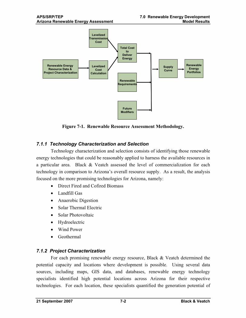
APS/SRP/TEPArizona Renewable Energy Assessment
7.0 Renewable Energy DevelopmentModel Results
21 September 2007 7-2 Black & Veatch
Renewable Energy Resource Data &
Project Characterization
Total Costto
DeliverEnergy
LevelizedTransmission
Cost
SupplyCurve
LevelizedCost
Calculation
FutureModifiers
RenewableRequirements
RenewableEnergy
Portfolios
Renewable Energy Resource Data &
Project Characterization
Total Costto
DeliverEnergy
LevelizedTransmission
Cost
SupplyCurve
LevelizedCost
Calculation
FutureModifiers
RenewableRequirements
RenewableEnergy
Portfolios
Figure 7-1. Renewable Resource Assessment Methodology.
7.1.1 Technology Characterization and Selection Technology characterization and selection consists of identifying those renewable
energy technologies that could be reasonably applied to harness the available resources in a particular area. Black & Veatch assessed the level of commercialization for each technology in comparison to Arizona’s overall resource supply. As a result, the analysis focused on the more promising technologies for Arizona, namely:
Direct Fired and Cofired Biomass Landfill Gas Anaerobic Digestion Solar Thermal Electric Solar Photovoltaic HydroelectricWind Power Geothermal
7.1.2 Project CharacterizationFor each promising renewable energy resource, Black & Veatch determined the
potential capacity and locations where development is possible. Using several data sources, including maps, GIS data, and databases, renewable energy technology specialists identified high potential locations across Arizona for their respective technologies. For each location, these specialists quantified the generation potential of
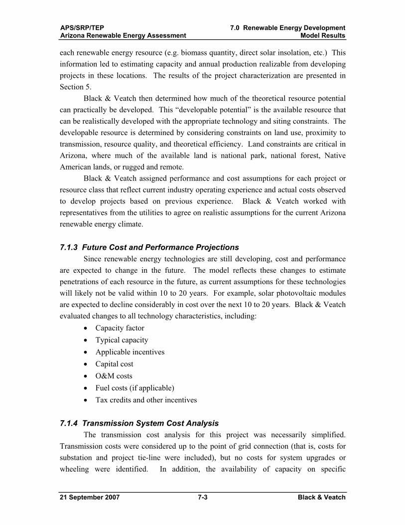
APS/SRP/TEPArizona Renewable Energy Assessment
7.0 Renewable Energy DevelopmentModel Results
21 September 2007 7-3 Black & Veatch
each renewable energy resource (e.g. biomass quantity, direct solar insolation, etc.) This information led to estimating capacity and annual production realizable from developing projects in these locations. The results of the project characterization are presented in Section 5.
Black & Veatch then determined how much of the theoretical resource potential can practically be developed. This “developable potential” is the available resource that can be realistically developed with the appropriate technology and siting constraints. The developable resource is determined by considering constraints on land use, proximity to transmission, resource quality, and theoretical efficiency. Land constraints are critical in Arizona, where much of the available land is national park, national forest, Native American lands, or rugged and remote.
Black & Veatch assigned performance and cost assumptions for each project or resource class that reflect current industry operating experience and actual costs observed to develop projects based on previous experience. Black & Veatch worked with representatives from the utilities to agree on realistic assumptions for the current Arizona renewable energy climate.
7.1.3 Future Cost and Performance Projections Since renewable energy technologies are still developing, cost and performance
are expected to change in the future. The model reflects these changes to estimate penetrations of each resource in the future, as current assumptions for these technologies will likely not be valid within 10 to 20 years. For example, solar photovoltaic modules are expected to decline considerably in cost over the next 10 to 20 years. Black & Veatch evaluated changes to all technology characteristics, including:
Capacity factor Typical capacity Applicable incentives Capital cost O&M costs Fuel costs (if applicable) Tax credits and other incentives
7.1.4 Transmission System Cost Analysis The transmission cost analysis for this project was necessarily simplified.
Transmission costs were considered up to the point of grid connection (that is, costs for substation and project tie-line were included), but no costs for system upgrades or wheeling were identified. In addition, the availability of capacity on specific

APS/SRP/TEPArizona Renewable Energy Assessment
7.0 Renewable Energy DevelopmentModel Results
21 September 2007 7-4 Black & Veatch
transmission lines was not assessed. Lines were assumed to have available capacity to accommodate the projects.
Based on input from the utilities, Black & Veatch estimated interconnection substation and transmission line spur costs for each potential project. Black & Veatch also identified the utility that corresponded to the service area and transmission line.
7.1.5 Levelized Cost of Electricity Calculations Black & Veatch calculated the levelized cost of electricity by using the
performance and cost assumptions for each project combined with the appropriate financing and economic assumptions for the type of development (see Table 7-3). The levelized cost is a measure of the life-cycle cost to generate electricity with a particular project. This cost allows various technologies, both conventional and renewable, to be compared on an equal economic basis ($/MWh). The methodology for levelized cost calculation is described in Section 4.1.
7.1.6 Supply Curve Development Black & Veatch developed supply curves for the aggregate mix of renewable
energy projects available to Arizona. Supply curves are used in economic analysis to determine the quantity of a product that is available for a particular price (e.g., the amount of renewable energy that can be generated within a utility system for under $50/MWh). The supply curve is constructed by plotting the amount of generation or capacity added by each technology or project against its corresponding levelized cost. For this study, the renewable generation added by each project class is plotted against its levelized cost of electricity in ascending order. As an example, see Figure 7-2. In this case, generation (GWh/yr) is on the x-axis and levelized cost ($/MWh) is shown on the y-axis. The supply curve shows that there are only a few projects that would be able to supply power for under $100/MWh by 2020. However, there is a large pool of solar resources at a cost of about $200/MWh.
APS/SRP/TEPArizona Renewable Energy Assessment
7.0 Renewable Energy DevelopmentModel Results
21 September 2007 7-5 Black & Veatch
0 5,000 10,000 15,000 20,0000
50
100
150
200
250
300
350
Generation, GWh
Leve
lized
Cos
t, $/
MW
hWindBiomass SolarHydroGeothermal
2020 Supply Curve
Figure 7-2. Arizona Resource Supply Curve.
Every “step” on the graph represents an individual project color-coded by its technology type. The curve compares the quantities and costs for the renewable resources and shows which products can be brought to market at the lowest cost (resources towards the left side). Supply curves were generated for each of the technologies under study (Section 5) and then combined.
Because a supply curve models potential projects, every year has a different supply curve. Due to time required for resource procurement, engineering, ACC approval, and construction, many projects are not feasibly available for energy production for several years. Of the many potential projects in Arizona, only a select few could be available over the next two years. However, by 2015, the majority of potential projects could feasibly be available. The further out the time horizon, the “longer” the supply curves become, representing a large pool of available generation.
As time proceeds, the lower cost renewable energy resources are most likely to be developed first, while higher price resources would likely be developed in future years. However, it is important to note that supply curves will change each year for variety of factors, including:
The least-cost projects are assumed to be developed first and can no longer be considered as part of the supply curves for new generation
APS/SRP/TEPArizona Renewable Energy Assessment
7.0 Renewable Energy DevelopmentModel Results
21 September 2007 7-6 Black & Veatch
Minimum project development timelines constrain project development (e.g., not all wind resource could be developed in 2009) Improvements in technology over time affect costs Commercial availability of new renewable technologies (e.g., dish engine solar in 2015) Timing of development of proposed transmission projects enabling development of new resources Expiration of tax credits and other incentives
The supply curves help the utilities determine the optimal mix of renewable energy to balance cost and generation. Importantly, however, there are numerous other factors to consider in addition to the generation cost shown in the supply curves. These are described below.
7.1.7 Model Limitations The model used for this report was a relatively simple linear model. The
renewable energy supply curves were developed based largely on best available public information and they represent a snapshot of what could be developed in the near term without consideration of significant future technology advancements. The projects identified, although based on analysis of best-available data, should be considered hypothetical but representative of actual projects that could be developed to meet renewable energy demand. In addition, the model has the following limitations, many of which were established by the agreed-upon scope of work for this project:
No resources were considered outside of Arizona (including existing power purchase agreements) No distributed generation resources were considered No banking of excess renewable generation was included to meet future demands. In addition there was no carry-forward of under-procurement. The transmission assessment has been simplified, as described previously. No consideration has been made for the differential value of different resources (avoided cost).Except for already announced projects (assumed to fail at a 50 percent rate), project failure was not explicitly modeled. No intra-annual variability of resources was considered.Costs to integrate intermittent resources (e.g., firming of wind) were not included. (Note, however, that wind comprises a relatively small portion of the portfolio. Solar projects largely include integrated thermal storage.)
APS/SRP/TEPArizona Renewable Energy Assessment
7.0 Renewable Energy DevelopmentModel Results
21 September 2007 7-7 Black & Veatch
The model is not a production cost model and does not simulate system dispatch.
In selecting projects to develop or procure, utilities may further consider these limitations, which may result in a different order of resource/project development than shown in the supply curves in this report. The most important additional factors that should be considered are competitiveness of out-of-state resources, transmission costs needed to access some resources (particularly wind), and the differential avoided cost (or value) of resources.
Consideration of avoided costs is particularly important. Avoided cost is typically determined by assessing a resource’s capacity value (based on degree of “firmness” at the time of a utility’s system peak demand) and its energy value (based on time of delivery). This is important when comparing resources such as wind and solar. For example, wind energy projects only provide fractional capacity value (often estimated at 20 percent or less of the nameplate capacity) and are more likely to offset low cost energy resources during the winter and spring. Solar resources can readily provide firm capacity with gas hybridization or thermal storage. Further, solar is generally coincident with times of higher energy needs, when less efficient (and more expensive) peaking resources are more likely to be offset.
There are numerous methods to calculate avoided cost, and costs are specific to individual utility systems. Figure 7-3 shows an example calculation for wind and solar. For wind, the following assumptions have been made:
Energy – offsets electricity from a natural gas combined cycle. The wind would offset the variable component of a combined cycle plant, which is the sum of the variable operations and maintenance cost and the fuel cost (heat rate times gas cost). Capacity – offsets 20 percent of the capacity of a natural gas simple cycle. The fixed carrying cost of a simple cycle has been assumed to be $100/kW-yr. Integration cost – the intermittent nature of wind results in higher system operations costs for utilities to integrate its varying output. This cost is generally relatively small at low levels of penetration. A value of $3.50/MWh has been assumed as an additional cost for wind.
For solar thermal (with natural gas back-up or integrated storage), the following assumptions have been made:
Energy – offsets electricity from a natural gas simple cycle.Capacity – offsets 100 percent of the capacity of a natural gas simple cycle.
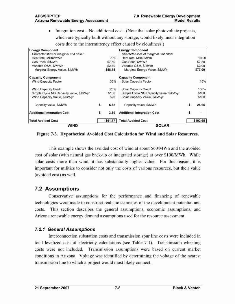
APS/SRP/TEPArizona Renewable Energy Assessment
7.0 Renewable Energy DevelopmentModel Results
21 September 2007 7-8 Black & Veatch
Integration cost – No additional cost. (Note that solar photovoltaic projects, which are typically built without any storage, would likely incur integration costs due to the intermittency effect caused by cloudiness.)
Energy ComponentCharacteristics of marginal unit offsetHeat rate, MBtu/MWh 7.50Gas Price, $/MWh $7.50Variable O&M, $/MWh $2.50
Marginal Energy Value, $/MWh $58.75
Capacity ComponentWind Capacity Factor 35%
Wind Capacity Credit 20%Simple Cycle NG Capacity value, $/kW-yr $100Wind Capacity Value, $/kW-yr $20
Capacity value, $/MWh 6.52$
Additional Integration Cost 3.50$
Total Avoided Cost $61.77
Energy ComponentCharacteristics of marginal unit offsetHeat rate, MBtu/MWh 10.00Gas Price, $/MWh $7.50Variable O&M, $/MWh $2.00
Marginal Energy Value, $/MWh $77.00
Capacity ComponentSolar Capacity Factor 45%
Solar Capacity Credit 100%Simple Cycle NG Capacity value, $/kW-yr $100Solar Capacity Value, $/kW-yr $100
Capacity value, $/MWh 25.65$
Additional Integration Cost -$
Total Avoided Cost $102.65 WIND SOLAR
Figure 7-3. Hypothetical Avoided Cost Calculation for Wind and Solar Resources.
This example shows the avoided cost of wind at about $60/MWh and the avoided cost of solar (with natural gas back-up or integrated storage) at over $100/MWh. While solar costs more than wind, it has substantially higher value. For this reason, it is important for utilities to consider not only the costs of various resources, but their value (avoided cost) as well.
7.2 Assumptions Conservative assumptions for the performance and financing of renewable
technologies were made to construct realistic estimates of the development potential and costs. This section describes the general assumptions, economic assumptions, and Arizona renewable energy demand assumptions used for the resource assessment.
7.2.1 General Assumptions Interconnection substation costs and transmission spur line costs were included in
total levelized cost of electricity calculations (see Table 7-1). Transmission wheeling costs were not included. Transmission assumptions were based on current market conditions in Arizona. Voltage was identified by determining the voltage of the nearest transmission line to which a project would most likely connect.
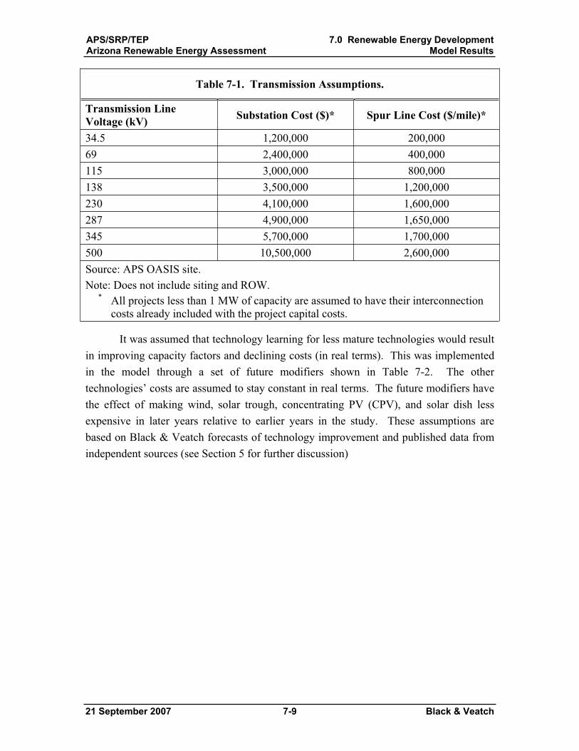
APS/SRP/TEPArizona Renewable Energy Assessment
7.0 Renewable Energy DevelopmentModel Results
21 September 2007 7-9 Black & Veatch
Table 7-1. Transmission Assumptions.
Transmission Line Voltage (kV) Substation Cost ($)* Spur Line Cost ($/mile)*
34.5 1,200,000 200,000 69 2,400,000 400,000 115 3,000,000 800,000 138 3,500,000 1,200,000 230 4,100,000 1,600,000 287 4,900,000 1,650,000 345 5,700,000 1,700,000 500 10,500,000 2,600,000 Source: APS OASIS site. Note: Does not include siting and ROW.
* All projects less than 1 MW of capacity are assumed to have their interconnection costs already included with the project capital costs.
It was assumed that technology learning for less mature technologies would result in improving capacity factors and declining costs (in real terms). This was implemented in the model through a set of future modifiers shown in Table 7-2. The other technologies’ costs are assumed to stay constant in real terms. The future modifiers have the effect of making wind, solar trough, concentrating PV (CPV), and solar dish less expensive in later years relative to earlier years in the study. These assumptions are based on Black & Veatch forecasts of technology improvement and published data from independent sources (see Section 5 for further discussion)
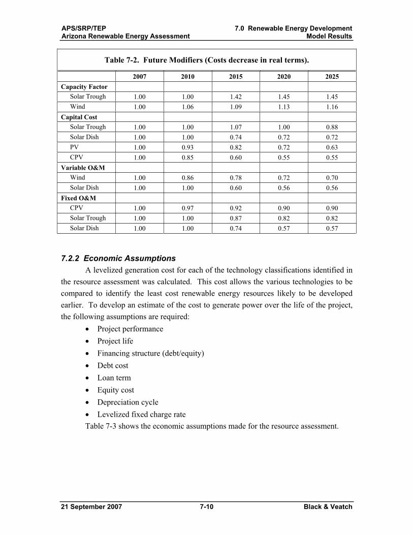
APS/SRP/TEPArizona Renewable Energy Assessment
7.0 Renewable Energy DevelopmentModel Results
21 September 2007 7-10 Black & Veatch
Table 7-2. Future Modifiers (Costs decrease in real terms).
2007 2010 2015 2020 2025 Capacity Factor
Solar Trough 1.00 1.00 1.42 1.45 1.45 Wind 1.00 1.06 1.09 1.13 1.16
Capital Cost Solar Trough 1.00 1.00 1.07 1.00 0.88 Solar Dish 1.00 1.00 0.74 0.72 0.72 PV 1.00 0.93 0.82 0.72 0.63 CPV 1.00 0.85 0.60 0.55 0.55
Variable O&M Wind 1.00 0.86 0.78 0.72 0.70 Solar Dish 1.00 1.00 0.60 0.56 0.56
Fixed O&M CPV 1.00 0.97 0.92 0.90 0.90 Solar Trough 1.00 1.00 0.87 0.82 0.82 Solar Dish 1.00 1.00 0.74 0.57 0.57
7.2.2 Economic Assumptions A levelized generation cost for each of the technology classifications identified in
the resource assessment was calculated. This cost allows the various technologies to be compared to identify the least cost renewable energy resources likely to be developed earlier. To develop an estimate of the cost to generate power over the life of the project, the following assumptions are required:
Project performance Project life Financing structure (debt/equity) Debt cost Loan term Equity cost Depreciation cycle Levelized fixed charge rate
Table 7-3 shows the economic assumptions made for the resource assessment.
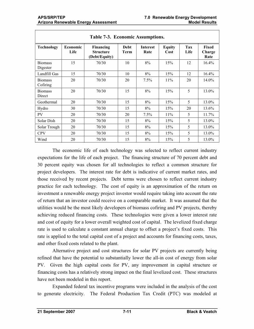
APS/SRP/TEPArizona Renewable Energy Assessment
7.0 Renewable Energy DevelopmentModel Results
21 September 2007 7-11 Black & Veatch
Table 7-3. Economic Assumptions.
Technology Economic Life
Financing Structure
(Debt/Equity)
Debt Term
Interest Rate
EquityCost
Tax Life
FixedCharge
Rate Biomass Digester
15 70/30 10 8% 15% 12 16.4%
Landfill Gas 15 70/30 10 8% 15% 12 16.4% Biomass Cofiring
20 70/30 20 7.5% 11% 20 14.0%
Biomass Direct
20 70/30 15 8% 15% 5 13.0%
Geothermal 20 70/30 15 8% 15% 5 13.0% Hydro 30 70/30 15 8% 15% 20 13.6% PV 20 70/30 20 7.5% 11% 5 11.7% Solar Dish 20 70/30 15 8% 15% 5 13.0% Solar Trough 20 70/30 15 8% 15% 5 13.0% CPV 20 70/30 15 8% 15% 5 13.0% Wind 20 70/30 15 8% 15% 5 13.0%
The economic life of each technology was selected to reflect current industry expectations for the life of each project. The financing structure of 70 percent debt and 30 percent equity was chosen for all technologies to reflect a common structure for project developers. The interest rate for debt is indicative of current market rates, and those received by recent projects. Debt terms were chosen to reflect current industry practice for each technology. The cost of equity is an approximation of the return on investment a renewable energy project investor would require taking into account the rate of return that an investor could receive on a comparable market. It was assumed that the utilities would be the most likely developers of biomass cofiring and PV projects, thereby achieving reduced financing costs. These technologies were given a lower interest rate and cost of equity for a lower overall weighted cost of capital. The levelized fixed charge rate is used to calculate a constant annual charge to offset a project’s fixed costs. This rate is applied to the total capital cost of a project and accounts for financing costs, taxes, and other fixed costs related to the plant.
Alternative project and cost structures for solar PV projects are currently being refined that have the potential to substantially lower the all-in cost of energy from solar PV. Given the high capital costs for PV, any improvement in capital structure or financing costs has a relatively strong impact on the final levelized cost. These structures have not been modeled in this report.
Expanded federal tax incentive programs were included in the analysis of the cost to generate electricity. The Federal Production Tax Credit (PTC) was modeled at
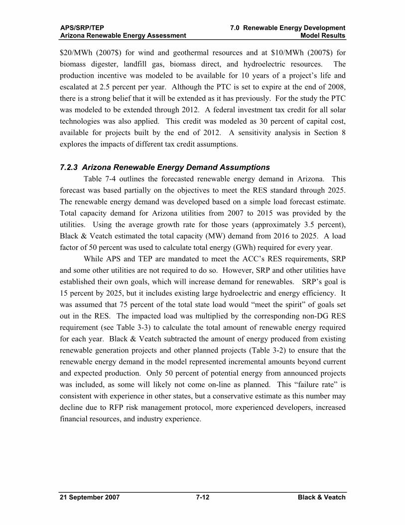
APS/SRP/TEPArizona Renewable Energy Assessment
7.0 Renewable Energy DevelopmentModel Results
21 September 2007 7-12 Black & Veatch
$20/MWh (2007$) for wind and geothermal resources and at $10/MWh (2007$) for biomass digester, landfill gas, biomass direct, and hydroelectric resources. The production incentive was modeled to be available for 10 years of a project’s life and escalated at 2.5 percent per year. Although the PTC is set to expire at the end of 2008, there is a strong belief that it will be extended as it has previously. For the study the PTC was modeled to be extended through 2012. A federal investment tax credit for all solar technologies was also applied. This credit was modeled as 30 percent of capital cost, available for projects built by the end of 2012. A sensitivity analysis in Section 8 explores the impacts of different tax credit assumptions.
7.2.3 Arizona Renewable Energy Demand Assumptions Table 7-4 outlines the forecasted renewable energy demand in Arizona. This
forecast was based partially on the objectives to meet the RES standard through 2025. The renewable energy demand was developed based on a simple load forecast estimate. Total capacity demand for Arizona utilities from 2007 to 2015 was provided by the utilities. Using the average growth rate for those years (approximately 3.5 percent), Black & Veatch estimated the total capacity (MW) demand from 2016 to 2025. A load factor of 50 percent was used to calculate total energy (GWh) required for every year.
While APS and TEP are mandated to meet the ACC’s RES requirements, SRP and some other utilities are not required to do so. However, SRP and other utilities have established their own goals, which will increase demand for renewables. SRP’s goal is 15 percent by 2025, but it includes existing large hydroelectric and energy efficiency. It was assumed that 75 percent of the total state load would “meet the spirit” of goals set out in the RES. The impacted load was multiplied by the corresponding non-DG RES requirement (see Table 3-3) to calculate the total amount of renewable energy required for each year. Black & Veatch subtracted the amount of energy produced from existing renewable generation projects and other planned projects (Table 3-2) to ensure that the renewable energy demand in the model represented incremental amounts beyond current and expected production. Only 50 percent of potential energy from announced projects was included, as some will likely not come on-line as planned. This “failure rate” is consistent with experience in other states, but a conservative estimate as this number may decline due to RFP risk management protocol, more experienced developers, increased financial resources, and industry experience.
APS/SRP/TEPArizona Renewable Energy Assessment
7.0 Renewable Energy DevelopmentModel Results
21 September 2007 7-13 Black & Veatch
Table 7-4. Arizona Renewable Energy Demand Forecast (Cumulative GWh).
Year Total Renewable Demand
Existing and Planned Projects
Net New Development
Required2007 884 312 572 2008 1,010 683 328 2009 1,128 825 303 2010 1,373 825 548 2011 1,597 825 773 2012 1,799 825 974 2013 2,126 825 1,302 2014 2,474 825 1,650 2015 2,844 825 2,019 2016 3,532 825 2,707 2017 4,265 825 3,440 2018 5,045 825 4,220 2019 5,874 825 5,049 2020 6,755 825 5,930 2021 7,691 825 6,866 2022 8,683 825 7,859 2023 9,736 825 8,912 2024 10,852 825 10,028 2025 12,034 825 11,210
7.3 Results The model was used to simulate the renewable resources that could be developed
to meet the 2025 demand of 11,210 GWh shown in Table 7-4. Although the model includes a variety of renewable energy resources that could be developed, other than solar, these resources appear relatively limited. In the mid to near-term, developable potential for new biomass, geothermal, and hydroelectric projects combined could contribute about 1,080 GWh/yr, or 1 percent of the electricity that was generated in Arizona in 2005. Wind could contribute about 2.5 percent. Despite the relatively limited potential of wind, biomass, geothermal and hydroelectric resources, they serve an important role in forestalling the need to install expensive solar. As such, their development may be important to keep renewable energy costs lower in the near term.
APS/SRP/TEPArizona Renewable Energy Assessment
7.0 Renewable Energy DevelopmentModel Results
21 September 2007 7-14 Black & Veatch
However, the relatively limited potential of these resources compared to surrounding states may serve as a deterrent for large, out-of-state renewable energy project developers.
Based on the resource assessments and future modifiers developed for each resource, supply curves were generated at annual increments from 2007 through 2025. Each supply curve was then compared against the total renewable energy demand required for each period. Supply curves for each year are provided in Appendix C. Figure 7-4 provides an example supply curve for 2015. This curve shows the Glen Canyon upgrade project the first year it is available as the lowest cost project (about $50/MWh). The potential demand line for 2015 crosses the supply line at the Glen Canyon project, indicating that Glen Canyon would likely be developed in 2015. The supply curve analysis was conducted under the assumption that each project would be developed and sold at its cost (including a reasonable developer profit), and not at the highest cost (“market clearing” price) in the respective period. This assumption is reasonable if it assumed that developers are pricing projects based on their costs and not unreasonably raising prices to take advantage of supply constraints in the market. This assumption is further examined in Section 8.
The projects selected for a particular year are removed from the next year’s supply curve. Thus, the supply curve in the last year does not represent a comprehensive supply curve of all resources available, but only those resources available for development at that time. It can be seen that the cost paid for renewable and advanced energy gradually increases as the lower cost resources are developed earlier in the RES term.
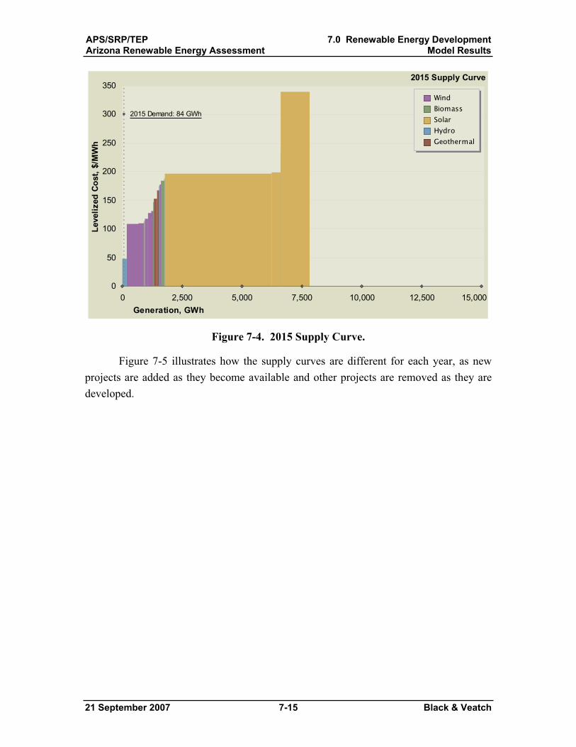
APS/SRP/TEPArizona Renewable Energy Assessment
7.0 Renewable Energy DevelopmentModel Results
21 September 2007 7-15 Black & Veatch
0 2,500 5,000 7,500 10,000 12,500 15,000
2015 Demand: 84 GWh
0
50
100
150
200
250
300
350
Generation, GWh
Leve
lized
Cos
t, $/
MW
hWindBiomass SolarHydroGeothermal
2015 Supply Curve
Figure 7-4. 2015 Supply Curve.
Figure 7-5 illustrates how the supply curves are different for each year, as new projects are added as they become available and other projects are removed as they are developed.
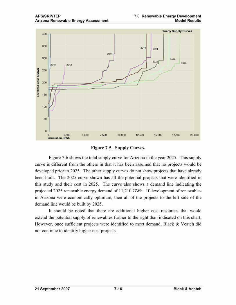
APS/SRP/TEPArizona Renewable Energy Assessment
7.0 Renewable Energy DevelopmentModel Results
21 September 2007 7-16 Black & Veatch
Yearly Supply Curves
2010 20202022
2012
2024
2014
2016
2018
0
50
100
150
200
250
300
350
400
0 2,500 5,000 7,500 10,000 12,500 15,000 17,500 20,000Generation, GWh
Leve
lized
Cos
t, $/
MW
h
Figure 7-5. Supply Curves.
Figure 7-6 shows the total supply curve for Arizona in the year 2025. This supply curve is different from the others in that it has been assumed that no projects would be developed prior to 2025. The other supply curves do not show projects that have already been built. The 2025 curve shown has all the potential projects that were identified in this study and their cost in 2025. The curve also shows a demand line indicating the projected 2025 renewable energy demand of 11,210 GWh. If development of renewables in Arizona were economically optimum, then all of the projects to the left side of the demand line would be built by 2025.
It should be noted that there are additional higher cost resources that would extend the potential supply of renewables further to the right than indicated on this chart. However, once sufficient projects were identified to meet demand, Black & Veatch did not continue to identify higher cost projects.
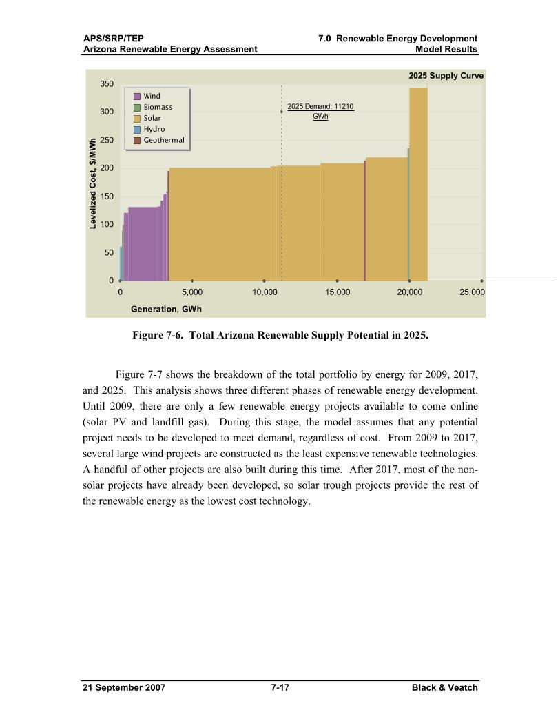
APS/SRP/TEPArizona Renewable Energy Assessment
7.0 Renewable Energy DevelopmentModel Results
21 September 2007 7-17 Black & Veatch
0 5,000 10,000 15,000 20,000 25,000
2025 Demand: 11210 GWh
0
50
100
150
200
250
300
350
Generation, GWh
Leve
lized
Cos
t, $/
MW
hWindBiomass SolarHydroGeothermal
2025 Supply Curve
Figure 7-6. Total Arizona Renewable Supply Potential in 2025.
Figure 7-7 shows the breakdown of the total portfolio by energy for 2009, 2017, and 2025. This analysis shows three different phases of renewable energy development. Until 2009, there are only a few renewable energy projects available to come online (solar PV and landfill gas). During this stage, the model assumes that any potential project needs to be developed to meet demand, regardless of cost. From 2009 to 2017, several large wind projects are constructed as the least expensive renewable technologies. A handful of other projects are also built during this time. After 2017, most of the non-solar projects have already been developed, so solar trough projects provide the rest of the renewable energy as the lowest cost technology.
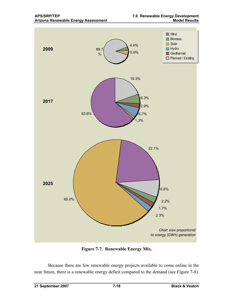
APS/SRP/TEPArizona Renewable Energy Assessment
7.0 Renewable Energy DevelopmentModel Results
21 September 2007 7-18 Black & Veatch
Chart size proportional to energy (GWh) generation
2.2%
1.7%
2.3%
65.0%
22.1%
6.6%
6.3%
2.9%
6.7%
1.3%
63.6%
19.3%
4.4%
5.9%89.7%
2009
2017
2025
WindBiomass SolarHydroGeothermalPlanned / Existing
Figure 7-7. Renewable Energy Mix.
Because there are few renewable energy projects available to come online in the near future, there is a renewable energy deficit compared to the demand (see Figure 7-8).
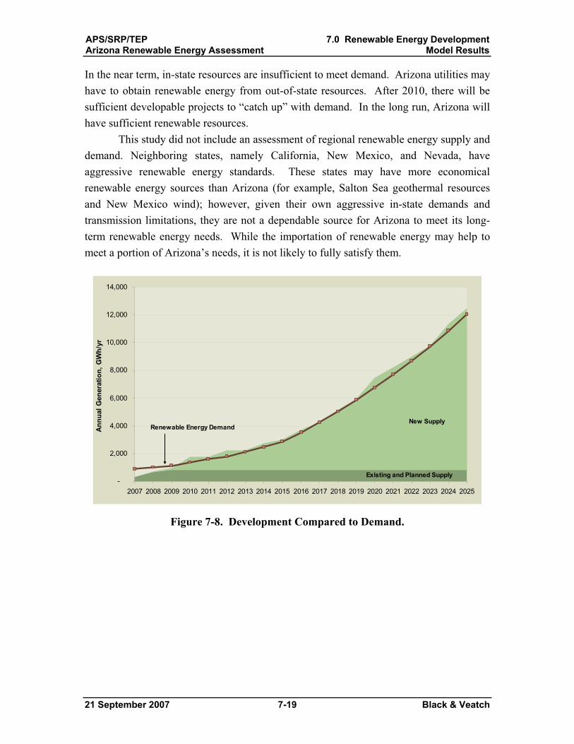
APS/SRP/TEPArizona Renewable Energy Assessment
7.0 Renewable Energy DevelopmentModel Results
21 September 2007 7-19 Black & Veatch
In the near term, in-state resources are insufficient to meet demand. Arizona utilities may have to obtain renewable energy from out-of-state resources. After 2010, there will be sufficient developable projects to “catch up” with demand. In the long run, Arizona will have sufficient renewable resources.
This study did not include an assessment of regional renewable energy supply and demand. Neighboring states, namely California, New Mexico, and Nevada, have aggressive renewable energy standards. These states may have more economical renewable energy sources than Arizona (for example, Salton Sea geothermal resources and New Mexico wind); however, given their own aggressive in-state demands and transmission limitations, they are not a dependable source for Arizona to meet its long-term renewable energy needs. While the importation of renewable energy may help to meet a portion of Arizona’s needs, it is not likely to fully satisfy them.
-
2,000
4,000
6,000
8,000
10,000
12,000
14,000
2007 2008 2009 2010 2011 2012 2013 2014 2015 2016 2017 2018 2019 2020 2021 2022 2023 2024 2025
Ann
ual G
ener
atio
n, G
Wh/
yr
Renewable Energy DemandNew Supply
Existing and Planned Supply
Figure 7-8. Development Compared to Demand.

APS/SRP/TEPArizona Renewable Energy Assessment
8.0 Assessment of Key RiskFactors
21 September 2007 8-1 Black & Veatch
8.0 Assessment of Key Risk Factors
Black & Veatch analyzed some of the risk factors of interest to utilities in Arizona to determine how sensitive the supply curve results would be to changing situations. These factors include tax credit changes, implementation of advanced solar technologies, delayed technical advances, escalating construction costs, manufacturing/supply chain constraints, near term performance learning curve, and competition for limited resources.
8.1 Sensitivity to Tax Credit Changes The base model assumes that the PTC and ITC will remain in place for another
five years, until 2012. Because these tax credits have a significant impact on the cost of power from renewable sources, two sensitivity runs were performed around this assumption:
Tax credits expire at the end of 2008 (current law) Tax credits never expire
Tax credits do not affect the availability of renewable resources, but they do impact the economics. In the long term, whether tax credits expire in 2008 or 2012 has surprisingly little impact on the cumulative average cost of meeting renewable energy demand in Arizona (less than 1 percent). This is because many of the most expensive, large solar projects would likely be built after 2012; they have the same cost under both scenarios. In the near term (through 2014), impacts are more significant. Costs are about 20 percent higher in the period 2009-2012. If tax credits never expire, the impact is significant. By 2025, the total renewable energy cost is about 25 percent lower than the base case assumption.
8.2 Advanced Solar Technologies Solar is the most expensive of the renewable resources profiled in this study. The
lower cost solar resources (about $180-205/MWh in 2007) are about twice as expensive as the bulk of the non-solar resources (about $70-110/MWh in 2007). The base case model included only proven, fully commercial solar technologies such as solar photovoltaics and solar thermal trough. Concentrating PV (CPV) and dish engine technologies have the potential to lower the cost of electricity from solar.
Figure 8-1 shows the forecasted levelized costs for representative solar projects included in the model (the large jump after 2012 is due to tax credit expiration). It can be seen that the solar photovoltaic technologies do not compete with the solar thermal technologies for large, centralized generation using the financing assumptions in the base case model (Section 7 describes the possibility of innovative financing approaches for
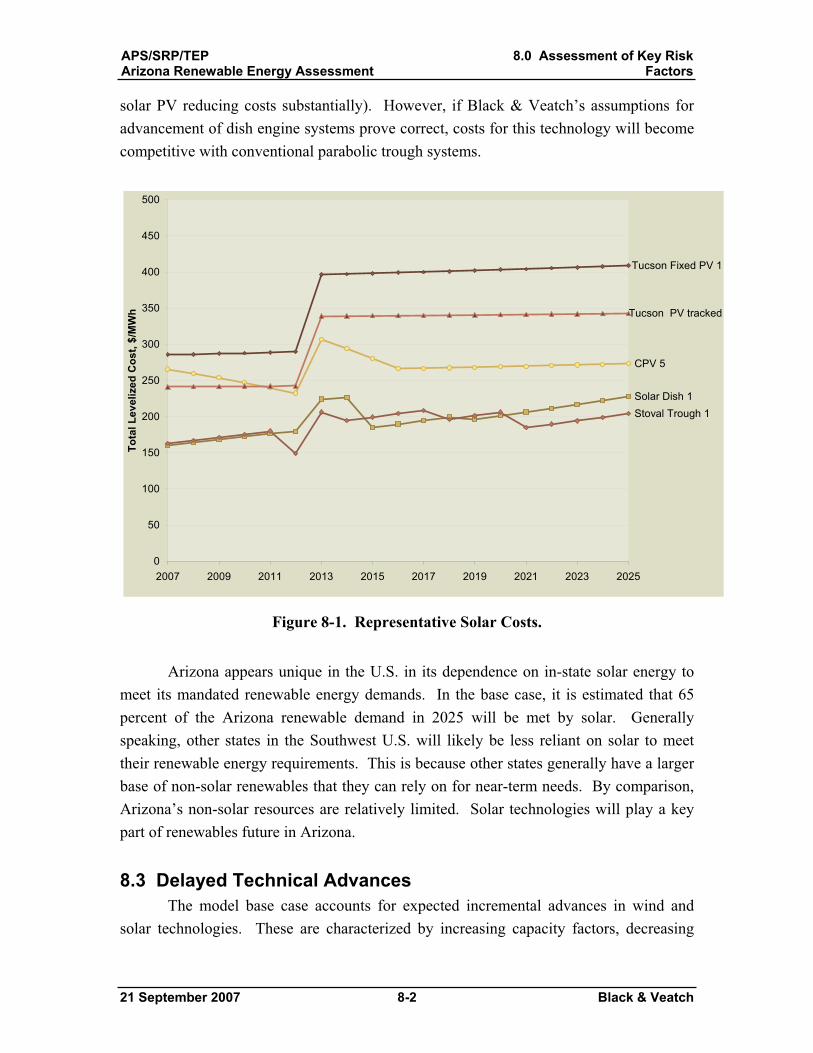
APS/SRP/TEPArizona Renewable Energy Assessment
8.0 Assessment of Key RiskFactors
21 September 2007 8-2 Black & Veatch
solar PV reducing costs substantially). However, if Black & Veatch’s assumptions for advancement of dish engine systems prove correct, costs for this technology will become competitive with conventional parabolic trough systems.
Tucson Fixed PV 1
Solar Dish 1
CPV 5
Stoval Trough 1
Tucson PV tracked
0
50
100
150
200
250
300
350
400
450
500
2007 2009 2011 2013 2015 2017 2019 2021 2023 2025
Tota
l Lev
eliz
ed C
ost,
$/M
Wh
Figure 8-1. Representative Solar Costs.
Arizona appears unique in the U.S. in its dependence on in-state solar energy to meet its mandated renewable energy demands. In the base case, it is estimated that 65 percent of the Arizona renewable demand in 2025 will be met by solar. Generally speaking, other states in the Southwest U.S. will likely be less reliant on solar to meet their renewable energy requirements. This is because other states generally have a larger base of non-solar renewables that they can rely on for near-term needs. By comparison, Arizona’s non-solar resources are relatively limited. Solar technologies will play a key part of renewables future in Arizona.
8.3 Delayed Technical Advances The model base case accounts for expected incremental advances in wind and
solar technologies. These are characterized by increasing capacity factors, decreasing
APS/SRP/TEPArizona Renewable Energy Assessment
8.0 Assessment of Key RiskFactors
21 September 2007 8-3 Black & Veatch
O&M costs, and falling capital costs for solar technologies. However, there is a risk that such advancement may be delayed or not realized. To assess the risk that wind and solar projects would experience delayed technical improvements, Black & Veatch reduced projected technology improvements in the model. To model no improvements in wind turbine design for wind projects, it was assumed that project capacity factors would not increase and O&M costs would not improve on a real basis. For solar thermal projects, it was assumed that capacity factor improvements due to storage would not be available until 2017 instead of 2012 and O&M costs would not improve on a real basis. For solar PV projects, it was assumed that capital costs would not improve on a real basis.
In this sensitivity analysis, wind and solar thermal projects were not as productive compared to the base case. Solar projects, particularly in the out years, are higher cost than the base case. The reduced technical advances will keep levelized costs for wind and solar higher, which will make other technologies (biomass and geothermal) comparatively more attractive in early years. The cumulative effect on the total renewable energy cost will likely be an increase of 15 to 20 percent by 2025. Overall, the delayed technical advances should not be expected to significantly alter the aggregate project mix. The general trend of exhausting nearly all potential biomass, wind, and hydroelectric, and geothermal projects before building solar trough projects holds true.
8.4 Escalating Construction Costs The model base case has a capital cost escalation of 2.5 percent, which is meant to
track close to general inflation. There is a risk that construction costs escalate at a higher rate, depending on future markets for materials and labor. For the sensitivity analysis of construction costs escalating faster than inflation, the capital cost escalator was changed to 5.0 percent.
Increasing the escalator increased levelized busbar costs for all projects. The increase is particularly pronounced for projects further into the future. At year 2025, levelized costs are about 37 percent higher than the base case.
8.5 Manufacturing and Supply Chain Constraints Manufacturing and supply chain constraints are already built into the model. The
projects most likely to be impacted by such constraints are solar and wind. For wind projects, there is currently a delay of up to two years between turbine order and turbine delivery because demand is greater than manufacturing capability. Wind projects were assigned “first year available” dates with this constraint in mind. The earliest any wind project is modeled to be available is 2010, with some not available until 2012 or 2013. If there are additional constraints in the wind supply chain, then it is likely that renewable
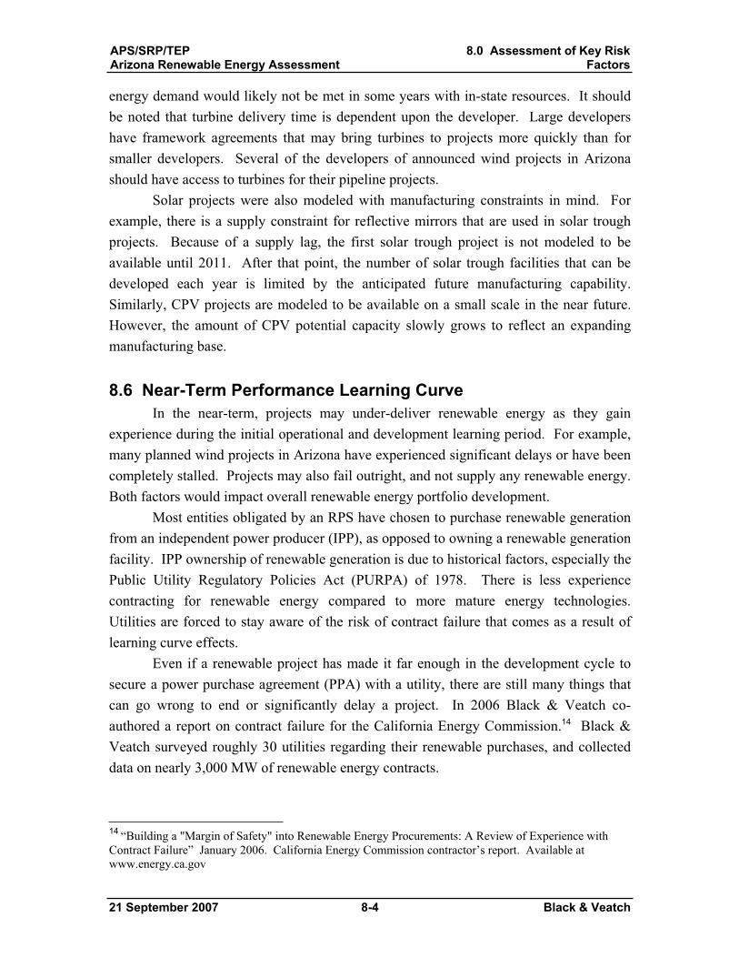
APS/SRP/TEPArizona Renewable Energy Assessment
8.0 Assessment of Key RiskFactors
21 September 2007 8-4 Black & Veatch
energy demand would likely not be met in some years with in-state resources. It should be noted that turbine delivery time is dependent upon the developer. Large developers have framework agreements that may bring turbines to projects more quickly than for smaller developers. Several of the developers of announced wind projects in Arizona should have access to turbines for their pipeline projects.
Solar projects were also modeled with manufacturing constraints in mind. For example, there is a supply constraint for reflective mirrors that are used in solar trough projects. Because of a supply lag, the first solar trough project is not modeled to be available until 2011. After that point, the number of solar trough facilities that can be developed each year is limited by the anticipated future manufacturing capability. Similarly, CPV projects are modeled to be available on a small scale in the near future. However, the amount of CPV potential capacity slowly grows to reflect an expanding manufacturing base.
8.6 Near-Term Performance Learning Curve In the near-term, projects may under-deliver renewable energy as they gain
experience during the initial operational and development learning period. For example, many planned wind projects in Arizona have experienced significant delays or have been completely stalled. Projects may also fail outright, and not supply any renewable energy. Both factors would impact overall renewable energy portfolio development.
Most entities obligated by an RPS have chosen to purchase renewable generation from an independent power producer (IPP), as opposed to owning a renewable generation facility. IPP ownership of renewable generation is due to historical factors, especially the Public Utility Regulatory Policies Act (PURPA) of 1978. There is less experience contracting for renewable energy compared to more mature energy technologies. Utilities are forced to stay aware of the risk of contract failure that comes as a result of learning curve effects.
Even if a renewable project has made it far enough in the development cycle to secure a power purchase agreement (PPA) with a utility, there are still many things that can go wrong to end or significantly delay a project. In 2006 Black & Veatch co-authored a report on contract failure for the California Energy Commission.14 Black & Veatch surveyed roughly 30 utilities regarding their renewable purchases, and collected data on nearly 3,000 MW of renewable energy contracts.
14 “Building a "Margin of Safety" into Renewable Energy Procurements: A Review of Experience with Contract Failure” January 2006. California Energy Commission contractor’s report. Available at www.energy.ca.gov
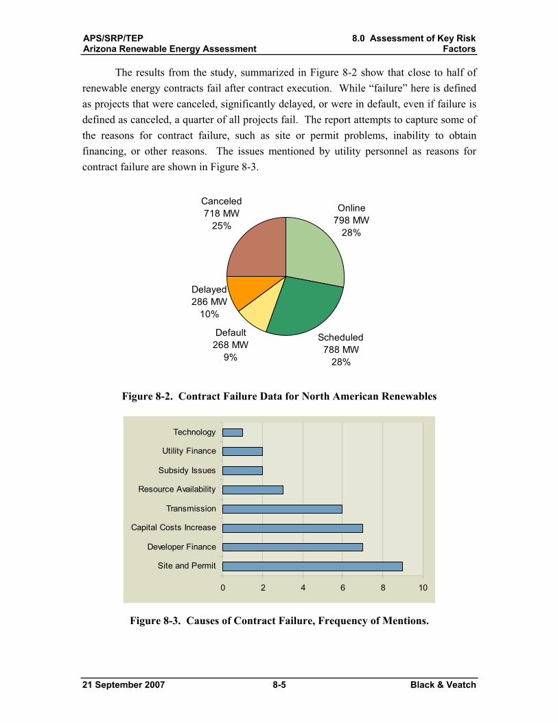
APS/SRP/TEPArizona Renewable Energy Assessment
8.0 Assessment of Key RiskFactors
21 September 2007 8-5 Black & Veatch
The results from the study, summarized in Figure 8-2 show that close to half of renewable energy contracts fail after contract execution. While “failure” here is defined as projects that were canceled, significantly delayed, or were in default, even if failure is defined as canceled, a quarter of all projects fail. The report attempts to capture some of the reasons for contract failure, such as site or permit problems, inability to obtain financing, or other reasons. The issues mentioned by utility personnel as reasons for contract failure are shown in Figure 8-3.
Online798 MW
28%
Default268 MW
9%
Delayed286 MW
10%
Canceled718 MW
25%
Scheduled788 MW
28%
Figure 8-2. Contract Failure Data for North American Renewables
0 2 4 6 8 10
Site and Permit
Developer Finance
Capital Costs Increase
Transmission
Resource Availability
Subsidy Issues
Utility Finance
Technology
Figure 8-3. Causes of Contract Failure, Frequency of Mentions.
APS/SRP/TEPArizona Renewable Energy Assessment
8.0 Assessment of Key RiskFactors
21 September 2007 8-6 Black & Veatch
Most, if not all, of the reasons renewable energy contracts fail are beyond the control of the utility, and some are beyond the control of the developer. No matter the cause, contract failure is a real problem for utilities trying to meet renewable energy demands.
To apply learning curve effects, it is important to understand that one of the reasons renewable energy contracts fail is a lack of experience with contracting for renewables. To mitigate this risk, utilities may “over-procure” renewable energy. For example, if a utility wanted renewable projects to produce 600 GWh for a certain year, the utility might enter into contract with projects for 800 GWh or more with the assumption that some projects would either be significantly delayed or never come online.
From a supply curve standpoint, contract failure and the utility counter measure of over-procurement serve to shift the supply curve to the left. When a project fails, its generation is removed from the supply curve, while all projects to the right (more expensive projects) shift left to fill in the space. As lower-priced projects fail, utilities will be forced to contract with more expensive renewable projects to secure renewable energy.
8.7 Competition for Limited Renewable Resources As more and more renewable energy projects are developed, there will be fewer
renewable resources to utilize in the future. There is a risk that utility competition for limited renewable resources will increase prices.
For renewable energy procurement, utilities typically contract with the least expensive energy available (projects on the left side of the supply curve). As renewable projects are developed, the supply curve shifts to the left. Utilities see an increasing marginal levelized cost as more expensive projects become the new lowest cost options. That is, costs increase as more renewable energy is developed. This is an expected phenomenon. However, there is a risk that IPPs will charge Arizona utilities the highest price possible that stays below the marginal cost of energy. Consider an example of a utility wanting to procure energy from three renewable energy projects for a certain year. The utility would have likely have several projects at different energy costs from which to choose. Other factors being equal, the three lowest priced projects would be chosen, with the most expensive project setting the marginal cost of energy (the most the utility is willing to pay at the time). If developers of the other two projects knew the utility’s marginal cost for renewables, they might be incented to raise their prices to the marginal cost to maximize profit. The utility would be forced to pay more for the energy, with no

APS/SRP/TEPArizona Renewable Energy Assessment
8.0 Assessment of Key RiskFactors
21 September 2007 8-7 Black & Veatch
other less expensive projects to pursue. This phenomenon occurs in supply constrained markets.
For Arizona utilities, it is possible that renewable energy developers may set energy prices as high as possible while still beating the marginal cost of energy. This would increase the price of power purchase agreements.
APS/SRP/TEPArizona Renewable Energy Assessment
Appendix A. Consolidated ProjectAssumptions
02 August 2007 A-1 Black & Veatch
Appendix A. Consolidated Project Assumptions
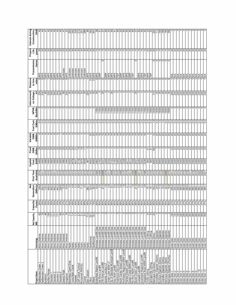
Proj
ect N
ame
Tech
nolo
gyNe
t Cap
acity
,MW
Cap
acity
Fact
or
Net
Gen
erat
ion,
GW
hr/y
rFi
rst Y
ear
Ava
ilabl
e
Cap
ital
Cos
t,$/
kW
Fixe
dO
&M
,$/
kWyr
Varia
ble
O&
M,
$/M
Whr
Fuel
Cos
t, $/
Mbt
uN
PHR
,B
tu/k
Whr
Inte
rcon
nect
ion
Vol
tage
, kV
Dis
tanc
eto
line
, m
iles
Tran
smis
sion
Ow
ner
Proj
ect
Life
,ye
ars
Inte
rest
dur
ing
Con
stru
ctio
n,$/
kWR
attle
snak
e C
rate
r 1W
ind
Ons
hore
6226
%13
8.8
2010
1600
259
0.0
023
00
AP
S20
45R
attle
snak
e C
rate
r 2W
ind
Ons
hore
7830
%20
2.5
2011
1600
258
0.0
023
00
AP
S20
45B
uckh
orn
Win
d O
nsho
re46
30%
119.
320
1016
8025
80.
00
697
AP
S20
47B
uffa
lo R
ange
Win
d O
nsho
re15
830
%40
9.0
2010
1600
258
0.0
023
01
AP
S20
45C
heve
lon
1W
ind
Ons
hore
171
30%
442.
220
1316
0025
80.
00
345
0A
PS
2045
Che
velo
n 2
Win
d O
nsho
re17
130
%44
2.2
2011
1600
258
0.0
034
50
AP
S20
45C
heve
lon
3W
ind
Ons
hore
171
30%
442.
220
1216
0025
80.
00
345
0A
PS
2045
Che
velo
n 4
Win
d O
nsho
re84
33%
238.
620
1016
0025
70.
00
345
0A
PS
2045
Gre
ens
Pea
kW
ind
Ons
hore
3127
%72
.820
1016
8025
80.
00
696
unkn
own
2047
Kin
gsto
neW
ind
Ons
hore
1827
%43
.820
1218
4025
80.
00
230
5A
PS
2052
Bea
rdsl
ey C
anal
Dro
pH
ydro
1.0
40%
3.5
2013
4324
246
0.0
035
1un
know
n30
363
Yum
a M
ain
Can
alH
ydro
1.4
40%
4.9
2013
4079
225
0.0
035
1un
know
n30
343
Wad
dell
Hyd
ro1.
540
%5.
320
1340
3721
50.
00
351
unkn
own
3033
9C
AP
Can
al T
urno
utH
ydro
2.5
40%
8.8
2013
3718
195
0.0
035
1un
know
n30
312
Roo
seve
lt (R
WC
D)
Hyd
ro3.
240
%11
.220
1335
7918
40.
00
351
unkn
own
3030
1Tu
cson
Hyd
ro0.
499
%3.
520
1334
2917
40.
00
351
unkn
own
3028
8G
len
Can
yon
Hyd
ro71
.845
%28
3.1
2015
997
82
0.0
023
01
AP
S30
84C
lifto
nG
eoth
erm
al20
.070
%12
2.6
2013
4000
030
0.0
035
10A
PS
2039
2G
illar
dG
eoth
erm
al15
.070
%92
.020
1445
000
300.
00
3510
AP
S20
441
But
terfi
eld
Sta
tion
Land
fill
Bio
mas
s La
ndfil
l Gas
280
%16
.920
0920
620
182.
011
500
350
AP
S15
58S
alt R
iver
Lan
dfill
Bio
mas
s La
ndfil
l Gas
180
%5.
520
0921
930
182.
011
500
00
SR
P15
6127
th A
venu
e La
ndfil
lB
iom
ass
Land
fill G
as3
80%
21.0
2050
2037
018
2.0
1150
035
00
1557
Apa
che
Junc
tion
LFB
iom
ass
Land
fill G
as0
80%
1.8
2010
2328
018
2.0
1150
00
0S
RP
1565
Cin
der L
ake
MS
W L
FB
iom
ass
Land
fill G
as1
80%
3.9
2011
2233
018
2.0
1150
00
0A
PS
1563
City
of G
lend
ale
Mun
icip
al L
andf
iBio
mas
s La
ndfil
l Gas
180
%9.
120
0921
320
182.
011
500
350
AP
S15
60G
rey
Wol
f Lan
dfill
Bio
mas
s La
ndfil
l Gas
180
%5.
520
1221
930
182.
011
500
00
AP
S15
61H
uach
uca
City
Lan
dfill
Bio
mas
s La
ndfil
l Gas
080
%2.
220
1223
050
182.
011
500
00
TEP
1565
Nor
th C
ente
r Stre
et L
andf
illB
iom
ass
Land
fill G
as1
80%
3.6
2008
2242
018
2.0
1150
00
0S
RP
1563
Nor
thw
est R
egio
nal M
SW
Lan
dfi lB
iom
ass
Land
fill G
as0
80%
1.8
2010
2328
018
2.0
1150
00
0A
PS
1565
Pai
nted
Des
ert L
andf
illB
iom
ass
Land
fill G
as0
80%
2.7
2010
2277
018
2.0
1150
00
0A
PS
1564
Que
en C
reek
MS
W L
andf
illB
iom
ass
Land
fill G
as0
80%
2.7
2011
2277
018
2.0
1150
00
0S
RP
1564
Rio
Ric
o M
SW
Lan
dfill
Bio
mas
s La
ndfil
l Gas
080
%1.
820
0823
280
182.
011
500
00
TEP
1565
Sku
nk C
reek
Lan
dfill
Bio
mas
s La
ndfil
l Gas
380
%21
.020
5020
370
182.
011
500
350
015
57C
ocop
ah L
andf
illB
iom
ass
Land
fill G
as1
80%
4.0
2011
2230
018
2.0
1150
00
0A
PS
1562
Sou
thw
est R
egio
nal L
andf
illB
iom
ass
Land
fill G
as0
80%
2.2
2010
2302
018
2.0
1150
00
0A
PS
1564
Tang
erin
e R
oad
MS
W L
andf
illB
iom
ass
Land
fill G
as1
80%
3.8
2008
2236
018
2.0
1150
00
0TE
P15
63C
holla
cof
iring
Bio
mas
s C
ofiri
ng10
80%
70.1
2010
900
610
2.5
1100
00
0A
PS
2024
Spr
inge
rvill
e co
firin
gB
iom
ass
Cof
iring
1080
%70
.120
1090
061
02.
310
000
00
TEP
2024
Mar
icop
a C
ity D
irect
Bio
mas
s D
irect
2080
%14
0.2
2012
4000
160
121.
914
500
115
20
2022
4S
now
flake
Dig
este
r (S
win
e)B
iom
ass
Dig
este
r4
80%
24.5
2010
2000
020
0.0
1500
035
00
1511
2B
ucke
ye D
iges
ter (
Dai
ry)
Bio
mas
s D
iges
ter
380
%17
.520
1030
000
201.
515
000
350
015
168
Cha
ndle
r Dig
este
r (D
airy
)B
iom
ass
Dig
este
r2
80%
10.5
2010
3500
020
1.5
1500
035
00
1519
6M
aric
opa
Dig
este
r (B
eef)
Bio
mas
s D
iges
ter
680
%42
.020
5035
000
200.
015
000
350
015
196
Mar
icop
a D
iges
ter (
Pou
ltry)
Bio
mas
s D
iges
ter
280
%16
.820
1030
000
200.
015
000
350
015
168
Sol
ar D
ish
1S
olar
Dis
h10
027
%24
0.0
2011
3300
2325
0.0
023
01
N/A
200
Sol
ar D
ish
2S
olar
Dis
h10
027
%24
0.0
2012
3300
2325
0.0
023
01
N/A
200
Sol
ar D
ish
3S
olar
Dis
h10
027
%24
0.0
2013
3300
2325
0.0
023
01
N/A
200
Sol
ar D
ish
4S
olar
Dis
h20
027
%48
0.0
2014
3300
2325
0.0
023
01
N/A
200
Sol
ar D
ish
5S
olar
Dis
h20
027
%48
0.0
2015
3300
2325
0.0
023
01
N/A
200
Sol
ar D
ish
6S
olar
Dis
h20
027
%48
0.0
2016
3300
2325
0.0
023
01
N/A
200
Sol
ar D
ish
7S
olar
Dis
h40
027
%96
0.1
2017
3300
2325
0.0
023
01
N/A
200
Sol
ar D
ish
8S
olar
Dis
h40
027
%96
0.1
2018
3300
2325
0.0
023
01
N/A
200
Sol
ar D
ish
9S
olar
Dis
h40
027
%96
0.1
2019
3300
2325
0.0
023
01
N/A
200
Sol
ar D
ish
10S
olar
Dis
h40
027
%96
0.1
2020
3300
2325
0.0
023
01
N/A
200
Sol
ar D
ish
11S
olar
Dis
h40
027
%96
0.1
2020
3300
2325
0.0
023
01
N/A
200
Sol
ar D
ish
12S
olar
Dis
h40
027
%96
0.1
2021
3300
2325
0.0
023
01
N/A
200
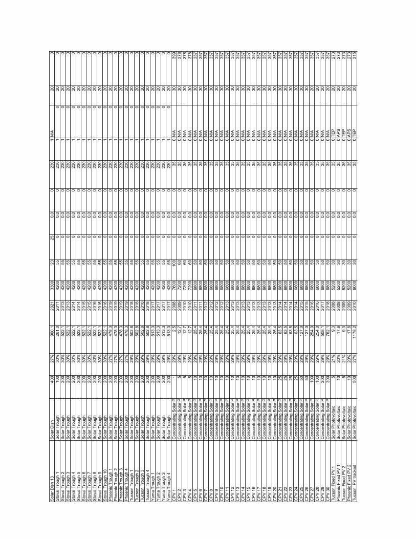
Sol
ar D
ish
13S
olar
Dis
h40
027
%96
0.1
2021
3300
2325
0.0
023
01
N/A
200
Sto
val T
roug
h 1
Sol
ar T
roug
h10
030
%26
1.0
2011
4200
550
0.0
023
01
020
0S
tova
l Tro
ugh
2S
olar
Tro
ugh
200
30%
522.
120
1342
0055
00.
00
230
10
200
Sto
val T
roug
h 3
Sol
ar T
roug
h20
030
%52
2.1
2013
4200
550
0.0
023
01
020
0S
tova
l Tro
ugh
4S
olar
Tro
ugh
200
30%
522.
120
1442
0055
00.
00
230
10
200
Sto
val T
roug
h 5
Sol
ar T
roug
h20
030
%52
2.1
2014
4200
550
0.0
023
01
020
0S
tova
l Tro
ugh
6S
olar
Tro
ugh
200
30%
522.
120
1542
0055
00.
00
230
10
200
Sto
val T
roug
h 7
Sol
ar T
roug
h20
030
%52
2.1
2015
4200
550
0.0
023
01
020
0S
tova
l Tro
ugh
8S
olar
Tro
ugh
200
30%
522.
120
1642
0055
00.
00
230
10
200
Sto
val T
roug
h 9
Sol
ar T
roug
h20
030
%52
2.1
2016
4200
550
0.0
023
01
020
0S
tova
l Tro
ugh
10S
olar
Tro
ugh
200
30%
522.
120
1642
0055
00.
00
230
10
200
Pho
enix
Tro
ugh
1S
olar
Tro
ugh
200
27%
478.
320
1942
0055
00.
00
230
10
200
Pho
enix
Tro
ugh
2S
olar
Tro
ugh
200
27%
478.
320
1942
0055
00.
00
230
10
200
Pho
enix
Tro
ugh
3S
olar
Tro
ugh
200
27%
478.
320
1942
0055
00.
00
230
10
200
Pho
enix
Tro
ugh
4S
olar
Tro
ugh
200
27%
478.
320
1942
0055
00.
00
230
10
200
Tucs
on T
roug
h 1
Sol
ar T
roug
h20
029
%50
2.8
2018
4200
550
0.0
023
01
020
0Tu
cson
Tro
ugh
2S
olar
Tro
ugh
200
29%
502.
820
1842
0055
00.
00
230
10
200
Tucs
on T
roug
h 3
Sol
ar T
roug
h20
029
%50
2.8
2018
4200
550
0.0
023
01
020
0Tu
cson
Tro
ugh
4S
olar
Tro
ugh
200
29%
502.
820
1842
0055
00.
00
230
10
200
Yum
a Tr
ough
1S
olar
Tro
ugh
200
29%
513.
320
1742
0055
00.
00
230
10
200
Yum
a Tr
ough
2S
olar
Tro
ugh
200
29%
513.
320
1742
0055
00.
00
230
10
200
Yum
a Tr
ough
3S
olar
Tro
ugh
200
29%
513.
320
1742
0055
00.
00
230
10
200
Yum
a Tr
ough
4S
olar
Tro
ugh
200
29%
513.
320
1742
0055
00.
00
230
10
200
CP
V 1
Con
cent
ratin
g S
olar
P1
29%
2.5
2008
7600
100
00.
00
350
N/A
3039
9C
PV
2C
once
ntra
ting
Sol
ar P
529
%12
.720
0972
0060
00.
00
350
N/A
3037
8C
PV
3C
once
ntra
ting
Sol
ar P
529
%12
.720
1072
0060
00.
00
350
N/A
3037
8C
PV
4C
once
ntra
ting
Sol
ar P
529
%12
.720
1072
0060
00.
00
350
N/A
3037
8C
PV
5C
once
ntra
ting
Sol
ar P
1029
%25
.420
1168
0050
00.
00
350
N/A
3035
7C
PV
6C
once
ntra
ting
Sol
ar P
1029
%25
.420
1168
0050
00.
00
350
N/A
3035
7C
PV
7C
once
ntra
ting
Sol
ar P
1029
%25
.420
1268
0050
00.
00
350
N/A
3035
7C
PV
8C
once
ntra
ting
Sol
ar P
1029
%25
.420
1268
0050
00.
00
350
N/A
3035
7C
PV
9C
once
ntra
ting
Sol
ar P
1029
%25
.420
1268
0050
00.
00
350
N/A
3035
7C
PV
10
Con
cent
ratin
g S
olar
P10
29%
25.4
2012
6800
500
0.0
035
0N
/A30
357
CP
V 1
1C
once
ntra
ting
Sol
ar P
1029
%25
.420
1368
0050
00.
00
350
N/A
3035
7C
PV
12
Con
cent
ratin
g S
olar
P10
29%
25.4
2013
6800
500
0.0
035
0N
/A30
357
CP
V 1
3C
once
ntra
ting
Sol
ar P
1029
%25
.420
1368
0050
00.
00
350
N/A
3035
7C
PV
14
Con
cent
ratin
g S
olar
P10
29%
25.4
2013
6800
500
0.0
035
0N
/A30
357
CP
V 1
5C
once
ntra
ting
Sol
ar P
1029
%25
.420
1368
0050
00.
00
350
N/A
3035
7C
PV
16
Con
cent
ratin
g S
olar
P10
29%
25.4
2013
6800
500
0.0
035
0N
/A30
357
CP
V 1
7C
once
ntra
ting
Sol
ar P
1029
%25
.420
1368
0050
00.
00
350
N/A
3035
7C
PV
18
Con
cent
ratin
g S
olar
P10
29%
25.4
2013
6800
500
0.0
035
0N
/A30
357
CP
V 1
9C
once
ntra
ting
Sol
ar P
1029
%25
.420
1368
0050
00.
00
350
N/A
3035
7C
PV
20
Con
cent
ratin
g S
olar
P10
29%
25.4
2013
6800
500
0.0
035
0N
/A30
357
CP
V 2
1C
once
ntra
ting
Sol
ar P
2529
%63
.520
1468
0050
00.
00
350
N/A
3035
7C
PV
22
Con
cent
ratin
g S
olar
P25
29%
63.5
2014
6800
500
0.0
035
0N
/A30
357
CP
V 2
3C
once
ntra
ting
Sol
ar P
2529
%63
.520
1468
0050
00.
00
350
N/A
3035
7C
PV
24
Con
cent
ratin
g S
olar
P25
29%
63.5
2014
6800
500
0.0
035
0N
/A30
357
CP
V 2
5C
once
ntra
ting
Sol
ar P
5029
%12
7.0
2015
6800
500
0.0
035
0N
/A30
357
CP
V 2
6C
once
ntra
ting
Sol
ar P
5029
%12
7.0
2015
6800
500
0.0
035
0N
/A30
357
CP
V 2
7C
once
ntra
ting
Sol
ar P
100
29%
254.
020
1668
0050
00.
00
350
N/A
2035
7C
PV
28
Con
cent
ratin
g S
olar
P10
029
%25
4.0
2016
6800
500
0.0
035
0N
/A20
357
CP
V 2
9C
once
ntra
ting
Sol
ar P
200
29%
508.
120
1768
0050
00.
00
350
N/A
2035
7C
PV
30
Con
cent
ratin
g S
olar
P30
029
%76
2.1
2018
6800
500
0.0
035
0N
/A20
357
Tucs
on F
ixed
PV
1S
olar
Pho
tovo
ltaic
521
%9.
320
0852
0030
00.
00
350
TEP
2027
3P
hoen
ix F
ixed
PV
1S
olar
Pho
tovo
ltaic
1020
%17
.620
0852
0030
00.
00
350
AP
S20
273
Tucs
on F
ixed
PV
2S
olar
Pho
tovo
ltaic
521
%9.
320
0952
0030
00.
00
350
TEP
2027
3P
hoen
ix F
ixed
PV
2S
olar
Pho
tovo
ltaic
1020
%17
.620
0952
0030
00.
00
350
AP
S20
273
Tucs
on P
V tr
acke
dS
olar
Pho
tovo
ltaic
500
27%
1178
.220
1060
0030
00.
00
350
TEP
2031
5
APS/SRP/TEPArizona Renewable Energy Assessment
Appendix B. Forecast Cost ofEnergy for Each Project
02 August 2007 B-1 Black & Veatch
Appendix B. Forecast Cost of Energy for Each Project
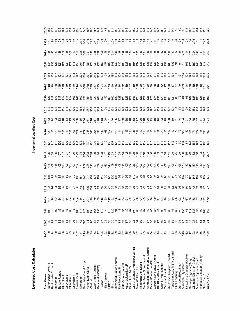
Leve
lized
Cos
t Cal
cula
tor
Proj
ect N
ame
2007
2008
2009
2010
2011
2012
2013
2014
2015
2016
2017
2018
2019
2020
2021
2022
2023
2024
2025
Rat
tlesn
ake
Cra
ter 1
9910
010
110
110
310
412
412
612
813
013
313
513
714
014
314
514
815
115
4R
attle
snak
e C
rate
r 284
8484
8586
8810
610
811
011
211
411
611
812
012
312
512
713
013
2B
uckh
orn
9091
9292
9495
114
116
118
120
123
125
127
129
132
134
137
140
142
Buf
falo
Ran
ge83
8383
8485
8710
510
710
911
111
311
511
711
912
112
412
612
913
1C
heve
lon
183
8383
8485
8610
510
710
911
111
311
511
711
912
112
412
612
813
1C
heve
lon
283
8383
8485
8610
510
710
911
111
311
511
711
912
112
412
612
813
1C
heve
lon
383
8383
8485
8610
510
710
911
111
311
511
711
912
112
412
612
813
1C
heve
lon
475
7676
7677
7997
9910
110
310
510
610
811
011
211
511
711
912
1G
reen
s P
eak
102
103
103
104
106
108
127
129
131
134
136
139
141
144
147
150
152
155
158
Kin
gsto
ne14
114
214
414
514
815
117
117
417
818
118
518
819
219
620
020
420
821
321
7B
eard
sley
Can
al D
rop
215
220
226
231
237
243
257
264
270
277
284
291
299
306
314
321
330
338
346
Yum
a M
ain
Can
al18
919
419
920
420
921
422
823
323
924
525
125
726
427
027
728
429
129
930
6W
adde
ll18
519
019
419
920
420
922
322
823
424
024
625
225
826
527
227
828
529
230
0C
AP
Can
al T
urno
ut15
816
216
617
017
417
819
119
620
120
621
121
622
222
723
323
924
525
125
7R
oose
velt
(RW
CD
)14
715
115
515
916
216
717
918
418
819
319
820
320
821
321
822
422
923
524
1Tu
cson
105
107
110
113
116
118
130
133
136
140
143
147
150
154
158
162
166
170
174
Gle
n C
anyo
n32
3334
3536
3646
4748
4950
5253
5456
5759
6062
Clif
ton
110
113
116
119
122
125
145
149
153
157
161
165
169
173
177
182
186
191
196
Gill
ard
122
125
128
132
135
138
159
163
167
171
176
180
185
189
194
199
204
209
214
But
terfi
eld
Sta
tion
Land
fill
8991
9496
9810
111
411
712
012
312
612
913
213
613
914
214
615
015
3S
alt R
iver
Lan
dfill
8284
8688
9193
106
108
111
114
117
120
123
126
129
132
135
139
142
27th
Ave
nue
Land
fill
8789
9194
9698
111
114
117
120
123
126
129
132
136
139
142
146
150
Apa
che
Junc
tion
LF85
8789
9194
9610
911
211
411
712
012
312
612
913
313
613
914
314
6C
inde
r Lak
e M
SW
LF
8385
8789
9194
107
109
112
115
118
121
124
127
130
133
137
140
143
City
of G
lend
ale
Mun
icip
al L
andf
ill99
102
104
107
109
112
125
129
132
135
138
142
145
149
153
157
161
165
169
Gre
y W
olf L
andf
ill82
8486
8891
9310
610
811
111
411
712
012
312
612
913
213
513
914
2H
uach
uca
City
Lan
dfill
8486
8991
9395
108
111
114
117
120
123
126
129
132
135
139
142
146
Nor
th C
ente
r Stre
et L
andf
ill83
8587
8992
9410
711
011
211
511
812
112
412
713
013
313
714
014
4N
orth
wes
t Reg
iona
l MS
W L
andf
ill85
8789
9194
9610
911
211
411
712
012
312
612
913
313
613
914
314
6P
aint
ed D
eser
t Lan
dfill
8486
8890
9295
108
110
113
116
119
122
125
128
131
134
138
141
145
Que
en C
reek
MS
W L
andf
ill84
8688
9092
9510
811
011
311
611
912
212
512
813
113
413
814
114
5R
io R
ico
MS
W L
andf
ill85
8789
9194
9610
911
211
411
712
012
312
612
913
313
613
914
314
6S
kunk
Cre
ek L
andf
ill87
8991
9496
9811
111
411
712
012
312
612
913
213
613
914
214
615
0C
ocop
ah L
andf
ill83
8587
8991
9410
710
911
211
511
812
112
412
713
013
313
614
014
3S
outh
wes
t Reg
iona
l Lan
dfill
8486
8991
9395
108
111
114
117
120
122
126
129
132
135
139
142
146
Tang
erin
e R
oad
MS
W L
andf
ill83
8587
8992
9410
710
911
211
511
812
112
412
713
013
313
714
014
4C
holla
cof
iring
6365
6668
7071
7375
7779
8183
8587
8991
9496
99S
prin
gerv
ille
cofir
ing
5859
6162
6465
6769
7072
7476
7879
8184
8688
90M
aric
opa
City
Dire
ct14
314
715
115
415
816
217
618
018
418
919
419
920
420
921
421
922
523
023
6S
now
flake
Dig
este
r (S
win
e)62
6465
6769
7082
8587
8991
9396
9810
010
310
610
811
1B
ucke
ye D
iges
ter (
Dai
ry)
112
115
117
120
123
126
140
143
147
151
154
158
162
166
170
175
179
184
188
Cha
ndle
r Dig
este
r (D
airy
)12
813
213
513
814
214
515
916
316
717
117
618
018
518
919
419
920
420
921
4M
aric
opa
Dig
este
r (B
eef)
9092
9597
9910
211
511
812
112
412
713
013
313
614
014
314
715
115
4M
aric
opa
Dig
este
r (P
oultr
y)86
8890
9295
9711
011
311
511
812
112
412
713
013
413
714
114
414
8S
olar
Dis
h 1
160
164
168
172
177
179
224
227
185
190
194
199
196
201
206
212
217
222
228
Sol
ar D
ish
216
016
416
817
217
717
922
422
718
519
019
419
919
620
120
621
221
722
222
8
Incr
emen
tal L
evel
ized
Cos
t

Sol
ar D
ish
316
016
416
817
217
717
922
422
718
519
019
419
919
620
120
621
221
722
222
8S
olar
Dis
h 4
158
162
166
171
175
177
222
225
183
188
192
197
194
199
204
209
214
220
225
Sol
ar D
ish
515
816
216
617
117
517
722
222
518
318
819
219
719
419
920
420
921
422
022
5S
olar
Dis
h 6
158
162
166
171
175
177
222
225
183
188
192
197
194
199
204
209
214
220
225
Sol
ar D
ish
715
816
216
617
017
417
622
122
418
218
719
119
619
319
820
320
821
321
922
4S
olar
Dis
h 8
158
162
166
170
174
176
221
224
182
187
191
196
193
198
203
208
213
219
224
Sol
ar D
ish
915
816
216
617
017
417
622
122
418
218
719
119
619
319
820
320
821
321
922
4S
olar
Dis
h 10
158
162
166
170
174
176
221
224
182
187
191
196
193
198
203
208
213
219
224
Sol
ar D
ish
1115
816
216
617
017
417
622
122
418
218
719
119
619
319
820
320
821
321
922
4S
olar
Dis
h 12
158
162
166
170
174
176
221
224
182
187
191
196
193
198
203
208
213
219
224
Sol
ar D
ish
1315
816
216
617
017
417
622
122
418
218
719
119
619
319
820
320
821
321
922
4S
tova
l Tro
ugh
116
316
717
117
518
014
920
619
419
920
420
819
620
120
618
518
919
419
920
4S
tova
l Tro
ugh
216
116
517
017
417
814
720
519
319
720
220
619
419
920
418
318
719
219
720
2S
tova
l Tro
ugh
316
116
517
017
417
814
720
519
319
720
220
619
419
920
418
318
719
219
720
2S
tova
l Tro
ugh
416
116
517
017
417
814
720
519
319
720
220
619
419
920
418
318
719
219
720
2S
tova
l Tro
ugh
516
116
517
017
417
814
720
519
319
720
220
619
419
920
418
318
719
219
720
2S
tova
l Tro
ugh
616
116
517
017
417
814
720
519
319
720
220
619
419
920
418
318
719
219
720
2S
tova
l Tro
ugh
716
116
517
017
417
814
720
519
319
720
220
619
419
920
418
318
719
219
720
2S
tova
l Tro
ugh
816
116
517
017
417
814
720
519
319
720
220
619
419
920
418
318
719
219
720
2S
tova
l Tro
ugh
916
116
517
017
417
814
720
519
319
720
220
619
419
920
418
318
719
219
720
2S
tova
l Tro
ugh
1016
116
517
017
417
814
720
519
319
720
220
619
419
920
418
318
719
219
720
2P
hoen
ix T
roug
h 1
176
181
185
190
194
160
223
210
216
221
225
212
217
223
199
204
210
215
220
Pho
enix
Tro
ugh
217
618
118
519
019
416
022
321
021
622
122
521
221
722
319
920
421
021
522
0P
hoen
ix T
roug
h 3
176
181
185
190
194
160
223
210
216
221
225
212
217
223
199
204
210
215
220
Pho
enix
Tro
ugh
417
618
118
519
019
416
022
321
021
622
122
521
221
722
319
920
421
021
522
0Tu
cson
Tro
ugh
116
817
217
618
018
515
321
220
020
521
021
420
220
721
219
019
419
920
420
9Tu
cson
Tro
ugh
216
817
217
618
018
515
321
220
020
521
021
420
220
721
219
019
419
920
420
9Tu
cson
Tro
ugh
316
817
217
618
018
515
321
220
020
521
021
420
220
721
219
019
419
920
420
9Tu
cson
Tro
ugh
416
817
217
618
018
515
321
220
020
521
021
420
220
721
219
019
419
920
420
9Y
uma
Trou
gh 1
164
168
172
177
181
149
208
196
201
206
210
197
202
207
186
190
195
200
205
Yum
a Tr
ough
216
416
817
217
718
114
920
819
620
120
621
019
720
220
718
619
019
520
020
5Y
uma
Trou
gh 3
164
168
172
177
181
149
208
196
201
206
210
197
202
207
186
190
195
200
205
Yum
a Tr
ough
416
416
817
217
718
114
920
819
620
120
621
019
720
220
718
619
019
520
020
5C
PV
137
637
136
636
135
534
843
242
040
739
439
640
040
340
641
041
441
742
142
5C
PV
229
128
527
927
226
525
733
532
230
829
329
429
529
629
729
830
030
130
230
4C
PV
329
128
527
927
226
525
733
532
230
829
329
429
529
629
729
830
030
130
230
4C
PV
429
128
527
927
226
525
733
532
230
829
329
429
529
629
729
830
030
130
230
4C
PV
526
626
025
424
724
023
330
629
428
026
626
726
726
826
927
027
127
127
227
3C
PV
626
626
025
424
724
023
330
629
428
026
626
726
726
826
927
027
127
127
227
3C
PV
726
626
025
424
724
023
330
629
428
026
626
726
726
826
927
027
127
127
227
3C
PV
826
626
025
424
724
023
330
629
428
026
626
726
726
826
927
027
127
127
227
3C
PV
926
626
025
424
724
023
330
629
428
026
626
726
726
826
927
027
127
127
227
3C
PV
10
266
260
254
247
240
233
306
294
280
266
267
267
268
269
270
271
271
272
273
CP
V 1
126
626
025
424
724
023
330
629
428
026
626
726
726
826
927
027
127
127
227
3C
PV
12
266
260
254
247
240
233
306
294
280
266
267
267
268
269
270
271
271
272
273
CP
V 1
326
626
025
424
724
023
330
629
428
026
626
726
726
826
927
027
127
127
227
3C
PV
14
266
260
254
247
240
233
306
294
280
266
267
267
268
269
270
271
271
272
273
CP
V 1
526
626
025
424
724
023
330
629
428
026
626
726
726
826
927
027
127
127
227
3C
PV
16
266
260
254
247
240
233
306
294
280
266
267
267
268
269
270
271
271
272
273
CP
V 1
726
626
025
424
724
023
330
629
428
026
626
726
726
826
927
027
127
127
227
3C
PV
18
266
260
254
247
240
233
306
294
280
266
267
267
268
269
270
271
271
272
273

CP
V 1
926
626
025
424
724
023
330
629
428
026
626
726
726
826
927
027
127
127
227
3C
PV
20
266
260
254
247
240
233
306
294
280
266
267
267
268
269
270
271
271
272
273
CP
V 2
126
225
625
024
323
622
830
228
927
626
126
226
226
326
326
426
526
626
626
7C
PV
22
262
256
250
243
236
228
302
289
276
261
262
262
263
263
264
265
266
266
267
CP
V 2
326
225
625
024
323
622
830
228
927
626
126
226
226
326
326
426
526
626
626
7C
PV
24
262
256
250
243
236
228
302
289
276
261
262
262
263
263
264
265
266
266
267
CP
V 2
526
025
524
824
223
422
730
028
827
426
026
026
026
126
226
226
326
426
426
5C
PV
26
260
255
248
242
234
227
300
288
274
260
260
260
261
262
262
263
264
264
265
CP
V 2
726
025
424
824
123
422
630
028
727
325
925
926
026
026
126
126
226
326
326
4C
PV
28
260
254
248
241
234
226
300
287
273
259
259
260
260
261
261
262
263
263
264
CP
V 2
925
925
424
724
123
322
629
928
627
325
825
925
926
026
026
126
226
226
326
4C
PV
30
259
254
247
240
233
226
299
286
273
258
258
259
260
260
261
261
262
263
263
Tucs
on F
ixed
PV
128
528
628
728
828
929
039
639
739
839
940
040
140
240
340
440
540
640
840
9P
hoen
ix F
ixed
PV
129
229
229
329
429
429
540
740
840
840
941
041
141
141
241
341
441
541
641
6Tu
cson
Fix
ed P
V 2
285
286
287
288
289
290
396
397
398
399
400
401
402
403
404
405
406
408
409
Pho
enix
Fix
ed P
V 2
292
292
293
294
294
295
407
408
408
409
410
411
411
412
413
414
415
416
416
Tucs
on P
V tr
acke
d24
124
124
224
224
224
233
933
934
034
034
034
034
134
134
134
234
234
334
3
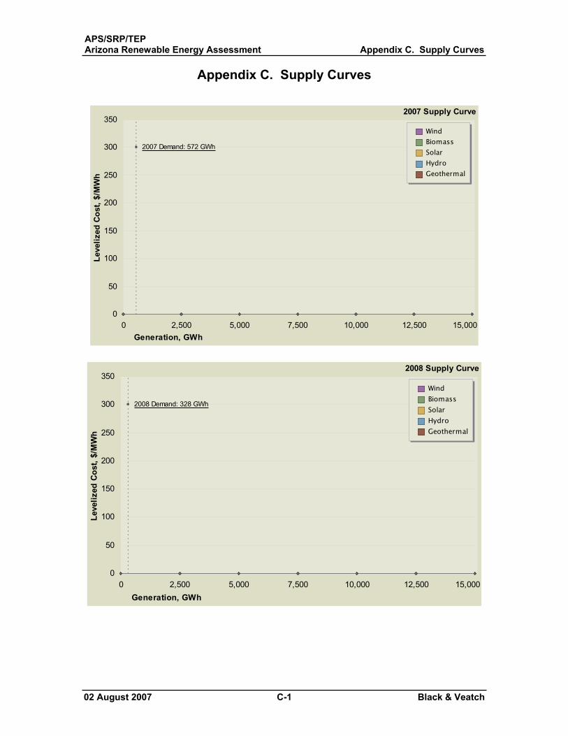
APS/SRP/TEPArizona Renewable Energy Assessment Appendix C. Supply Curves
02 August 2007 C-1 Black & Veatch
Appendix C. Supply Curves
0 2,500 5,000 7,500 10,000 12,500 15,000
2007 Demand: 572 GWh
0
50
100
150
200
250
300
350
Generation, GWh
Leve
lized
Cos
t, $/
MW
h
WindBiomass SolarHydroGeothermal
2007 Supply Curve
0 2,500 5,000 7,500 10,000 12,500 15,000
2008 Demand: 328 GWh
0
50
100
150
200
250
300
350
Generation, GWh
Leve
lized
Cos
t, $/
MW
h
WindBiomass SolarHydroGeothermal
2008 Supply Curve
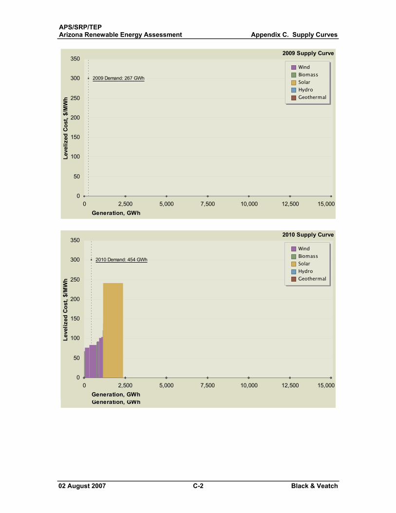
APS/SRP/TEPArizona Renewable Energy Assessment Appendix C. Supply Curves
02 August 2007 C-2 Black & Veatch
0 2,500 5,000 7,500 10,000 12,500 15,000
2009 Demand: 267 GWh
0
50
100
150
200
250
300
350
Generation, GWh
Leve
lized
Cos
t, $/
MW
hWindBiomass SolarHydroGeothermal
2009 Supply Curve
0 2,500 5,000 7,500 10,000 12,500 15,0000
50
100
150
200
250
300
350
Generation, GWh
Leve
lized
Cos
t, $/
MW
h
WindBiomass SolarHydroGeothermal
2011 Supply Curve
0 2,500 5,000 7,500 10,000 12,500 15,000
2010 Demand: 454 GWh
0
50
100
150
200
250
300
350
Generation, GWh
Leve
lized
Cos
t, $/
MW
h
WindBiomass SolarHydroGeothermal
2010 Supply Curve
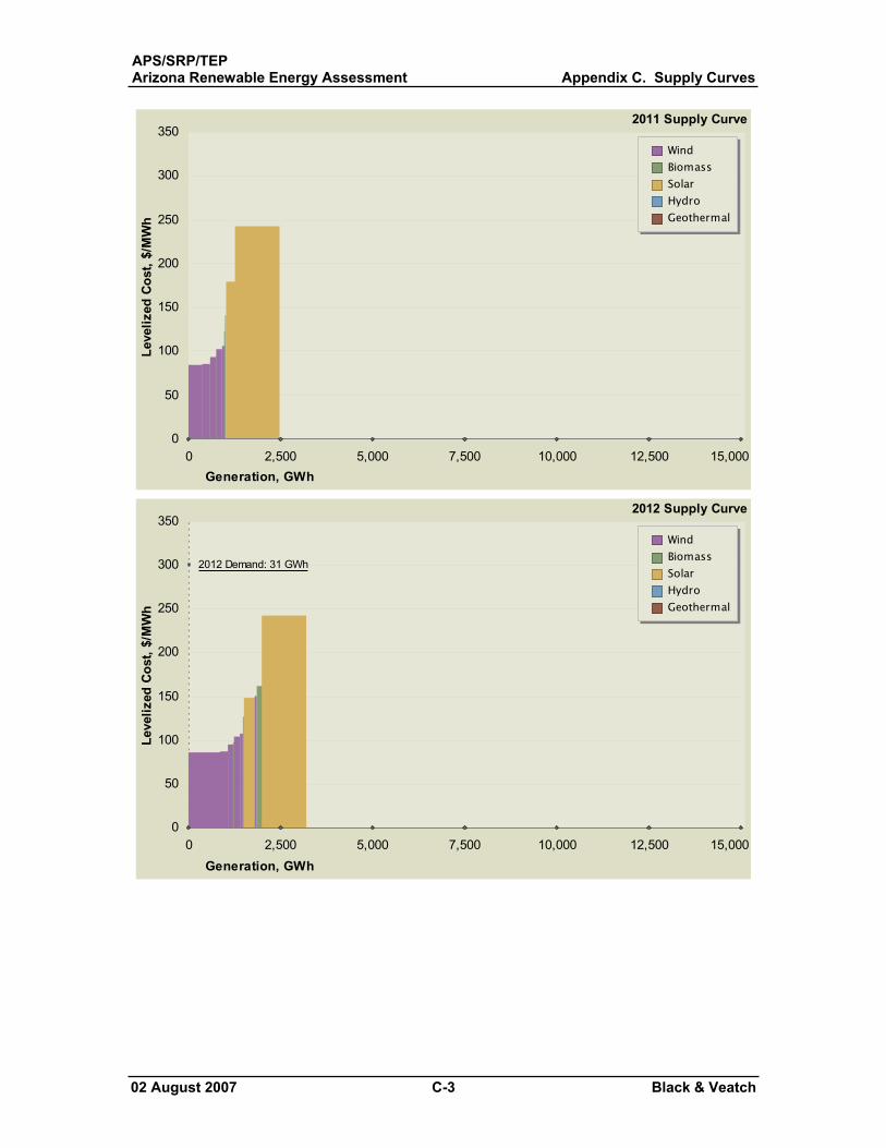
APS/SRP/TEPArizona Renewable Energy Assessment Appendix C. Supply Curves
02 August 2007 C-3 Black & Veatch
0 2,500 5,000 7,500 10,000 12,500 15,0000
50
100
150
200
250
300
350
Generation, GWh
Leve
lized
Cos
t, $/
MW
hWindBiomass SolarHydroGeothermal
2011 Supply Curve
0 2,500 5,000 7,500 10,000 12,500 15,000
2012 Demand: 31 GWh
0
50
100
150
200
250
300
350
Generation, GWh
Leve
lized
Cos
t, $/
MW
h
WindBiomass SolarHydroGeothermal
2012 Supply Curve
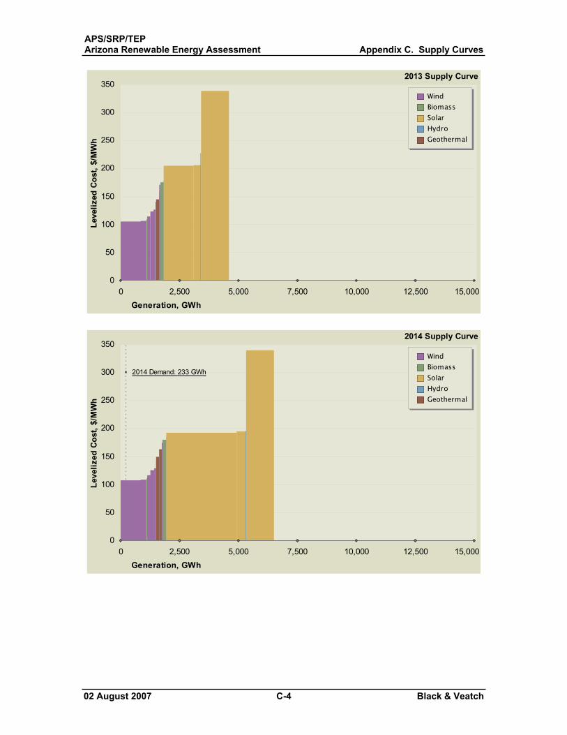
APS/SRP/TEPArizona Renewable Energy Assessment Appendix C. Supply Curves
02 August 2007 C-4 Black & Veatch
0 2,500 5,000 7,500 10,000 12,500 15,0000
50
100
150
200
250
300
350
Generation, GWh
Leve
lized
Cos
t, $/
MW
hWindBiomass SolarHydroGeothermal
2013 Supply Curve
0 2,500 5,000 7,500 10,000 12,500 15,000
2014 Demand: 233 GWh
0
50
100
150
200
250
300
350
Generation, GWh
Leve
lized
Cos
t, $/
MW
h
WindBiomass SolarHydroGeothermal
2014 Supply Curve
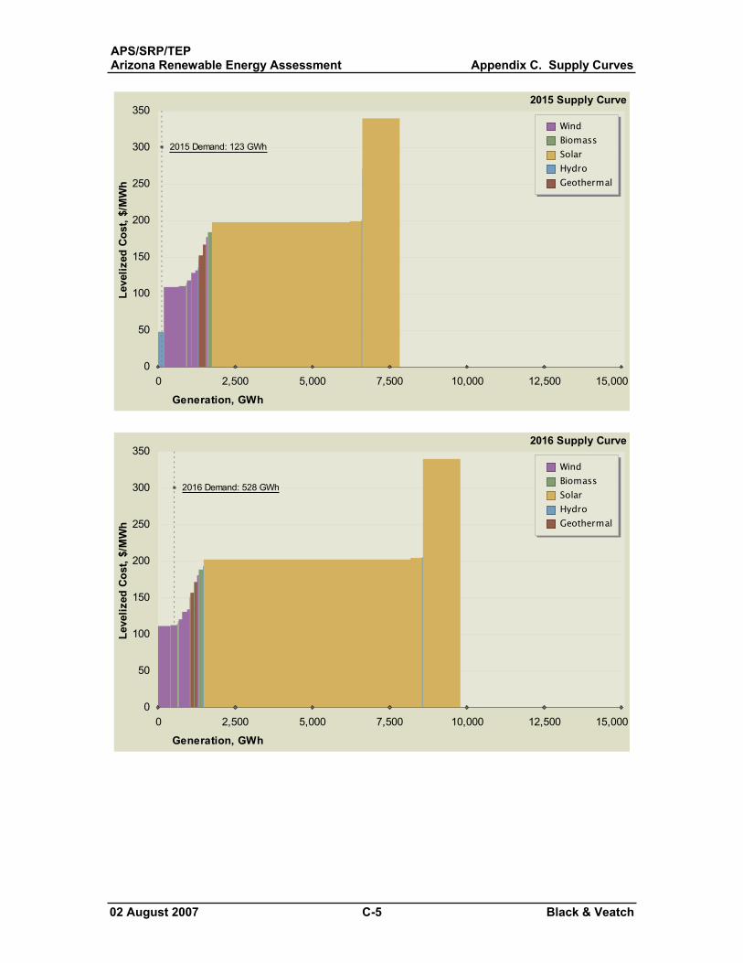
APS/SRP/TEPArizona Renewable Energy Assessment Appendix C. Supply Curves
02 August 2007 C-5 Black & Veatch
0 2,500 5,000 7,500 10,000 12,500 15,000
2015 Demand: 123 GWh
0
50
100
150
200
250
300
350
Generation, GWh
Leve
lized
Cos
t, $/
MW
hWindBiomass SolarHydroGeothermal
2015 Supply Curve
0 2,500 5,000 7,500 10,000 12,500 15,000
2016 Demand: 528 GWh
0
50
100
150
200
250
300
350
Generation, GWh
Leve
lized
Cos
t, $/
MW
h
WindBiomass SolarHydroGeothermal
2016 Supply Curve
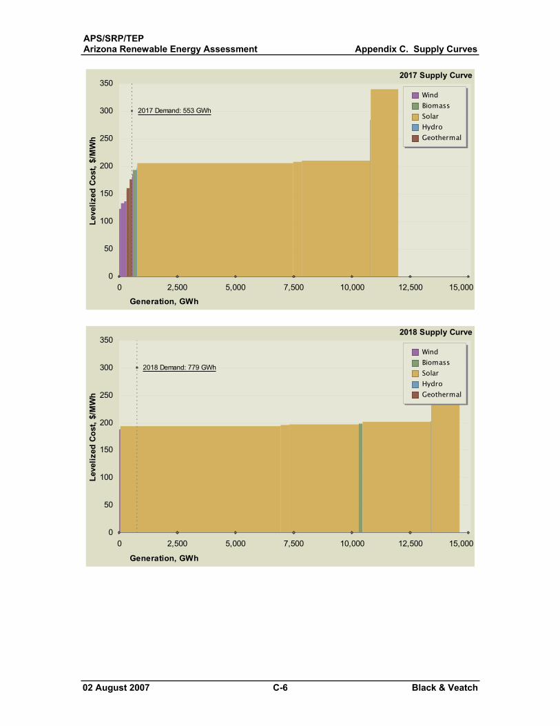
APS/SRP/TEPArizona Renewable Energy Assessment Appendix C. Supply Curves
02 August 2007 C-6 Black & Veatch
0 2,500 5,000 7,500 10,000 12,500 15,000
2017 Demand: 553 GWh
0
50
100
150
200
250
300
350
Generation, GWh
Leve
lized
Cos
t, $/
MW
hWindBiomass SolarHydroGeothermal
2017 Supply Curve
0 2,500 5,000 7,500 10,000 12,500 15,000
2018 Demand: 779 GWh
0
50
100
150
200
250
300
350
Generation, GWh
Leve
lized
Cos
t, $/
MW
h
WindBiomass SolarHydroGeothermal
2018 Supply Curve
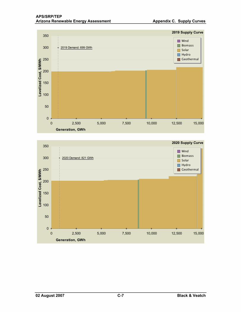
APS/SRP/TEPArizona Renewable Energy Assessment Appendix C. Supply Curves
02 August 2007 C-7 Black & Veatch
0 2,500 5,000 7,500 10,000 12,500 15,000
2019 Demand: 699 GWh
0
50
100
150
200
250
300
350
Generation, GWh
Leve
lized
Cos
t, $/
MW
hWindBiomass SolarHydroGeothermal
2019 Supply Curve
0 2,500 5,000 7,500 10,000 12,500 15,000
2020 Demand: 821 GWh
0
50
100
150
200
250
300
350
Generation, GWh
Leve
lized
Cos
t, $/
MW
h
WindBiomass SolarHydroGeothermal
2020 Supply Curve
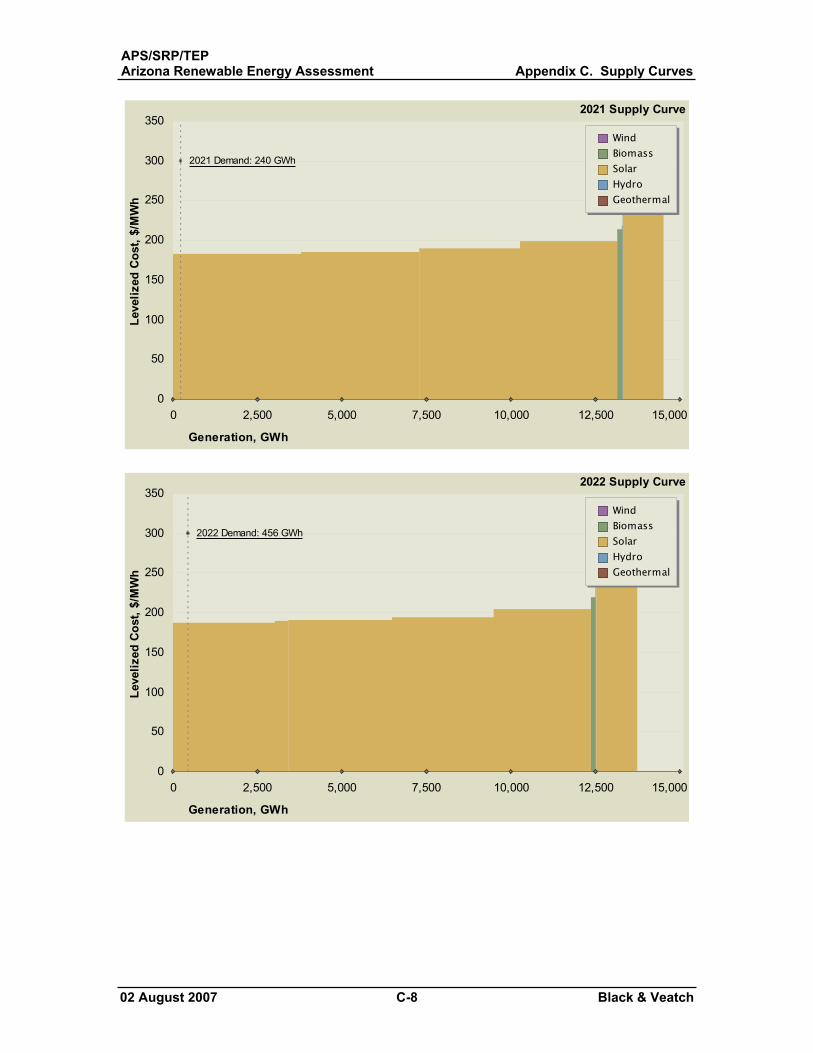
APS/SRP/TEPArizona Renewable Energy Assessment Appendix C. Supply Curves
02 August 2007 C-8 Black & Veatch
0 2,500 5,000 7,500 10,000 12,500 15,000
2021 Demand: 240 GWh
0
50
100
150
200
250
300
350
Generation, GWh
Leve
lized
Cos
t, $/
MW
hWindBiomass SolarHydroGeothermal
2021 Supply Curve
0 2,500 5,000 7,500 10,000 12,500 15,000
2022 Demand: 456 GWh
0
50
100
150
200
250
300
350
Generation, GWh
Leve
lized
Cos
t, $/
MW
h
WindBiomass SolarHydroGeothermal
2022 Supply Curve
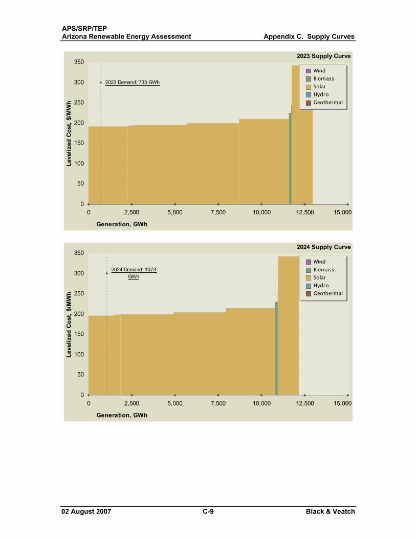
APS/SRP/TEPArizona Renewable Energy Assessment Appendix C. Supply Curves
02 August 2007 C-9 Black & Veatch
0 2,500 5,000 7,500 10,000 12,500 15,000
2023 Demand: 733 GWh
0
50
100
150
200
250
300
350
Generation, GWh
Leve
lized
Cos
t, $/
MW
hWindBiomass SolarHydroGeothermal
2023 Supply Curve
0 2,500 5,000 7,500 10,000 12,500 15,000
2024 Demand: 1073 GWh
0
50
100
150
200
250
300
350
Generation, GWh
Leve
lized
Cos
t, $/
MW
h
WindBiomass SolarHydroGeothermal
2024 Supply Curve
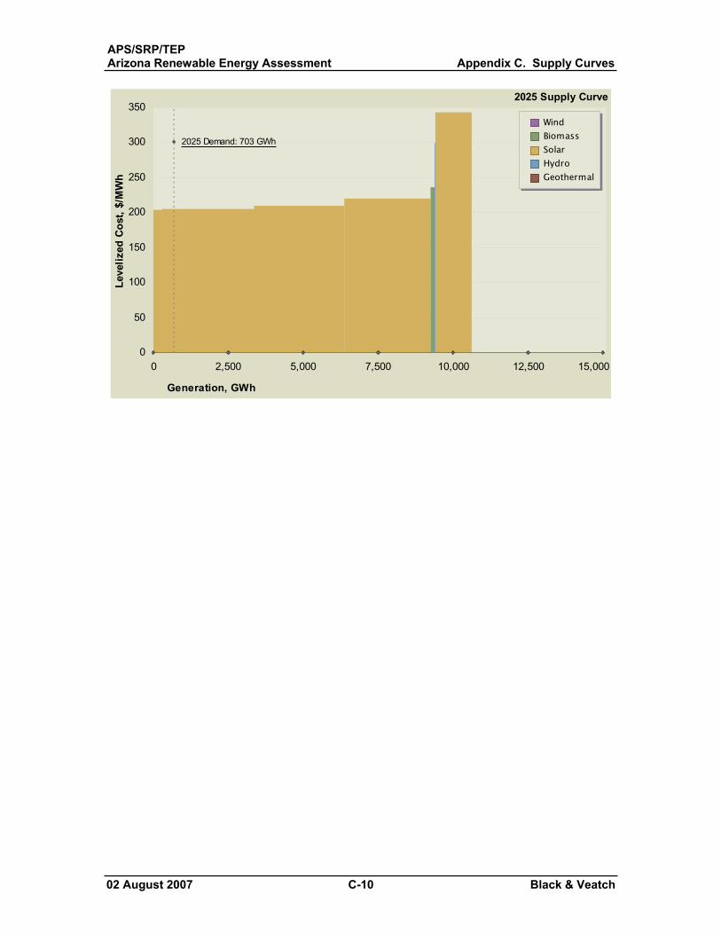
APS/SRP/TEPArizona Renewable Energy Assessment Appendix C. Supply Curves
02 August 2007 C-10 Black & Veatch
0 2,500 5,000 7,500 10,000 12,500 15,000
2025 Demand: 703 GWh
0
50
100
150
200
250
300
350
Generation, GWh
Leve
lized
Cos
t, $/
MW
hWindBiomass SolarHydroGeothermal
2025 Supply Curve