are political markets really superior to polls as election ... · are political markets really...

Are Political Markets Really Superior to Polls as Election Predictors?*

August 31, 2005

Robert S. Erikson Christopher Wlezien Columbia University Oxford University [email protected] [email protected]

Abstract Election markets have been praised for their ability to forecast elections, and to forecast even better than the polls. This paper challenges that argument, based on an analysis of Iowa Electronic Market (IEM) data from recent presidential elections. We show that while vote-share market prices do forecast better than naïve one-to-one interpretation of poll results, polls that are properly discounted for the favorite’s inflated lead outperform the market. Moreover, winner-take-all market prices predict poorly compared to reasonable win-projections based on the polls. Election markets generally see more uncertainty ahead in the campaign than the polling numbers warrant. The reasons for the poor performance of the IEM election markets are discussed. * Prepared for presentation at the Annual Meeting of the World Association of Public Opinion Research, Cannes, September, 2005. Research for this project was supported by National Science Foundation Grant SBR-9731308. We thank John Kastellec for his research assistance.

1

Election markets have recently emerged as an intriguing new tool for predicting

elections. These markets—made possible by the internet—now present the possibility that

electoral trends can be discerned well in advance by simply consulting the candidates’ latest

market prices. Or at least, that is a popular belief.

Modern political markets originated with the 1988 launching by the Business School at

the University of Iowa of its Iowa Electronic Market (IEM). The first IEM market was a

“vote-share” market for the 1988 Bush-Dukakis presidential contest, in which internet traders

electronically buy and sell futures contracts based on their forecasts of the candidates’ actual

vote percentages. Since 1992, IEM offers both a “vote-share” market and a higher-volume

“winner-take-all” presidential market, in which payoffs go to contracts on the popular vote

winner.1 Along the way, IEM has offered occasional markets on non-presidential races. Most

recently, commercial political markets on the internet have entered the field. Most notable is

the tradesport.com winner-take-all market on the 2004 US presidential election. Unlike IEM,

which has a $500 limit on individual investments, Tradesport.com has no limit on the amount

invested, making it the thicker and arguably more efficient market.2

Election markets have drawn considerable favor in both the popular and academic press

as an alternative to public opinion polls as a method of predicting elections. As James

1 In the IEM vote-share markets, one share of a candidate pays off in proportion to the candidate’s final vote share. For instance, one unit of a candidate who obtains 44 percent of the vote is worth pays 44 cents. A portfolio of one unit of each candidate pays exactly one dollar. A candidate’s unit price therefore represents the market’s expectation of the final vote. If a trader buys a candidate at, say, 40 cents per unit, and the candidate wins the 44 percent as in our example above, the profit is 4 cents on the dollar. If our trader buys at 40 and sells at 50, the profit is 10 cents on the dollar. In the IEM winner-take-all market, one share of a candidate pays off one dollar if the candidate wins and nothing if the candidate loses. A portfolio of one unit of each candidate pays exactly one dollar. A trader who buys one unit of a candidate at, say 40 cents on the dollar, wins either one dollar (a 60 cent profit) or nothing (a 40 cent loss) if the contract is held until market closing following the election. If our trader buys at 40 cents and sells at, say 60, the profit is 20 cents on the dollar. For further details, consult the IEM website, http://www.biz.uiowa.edu/iem/. 2 These “modern” election markets were not the first. Before the development of scientific polling, high-volume Wall Street election markets were an important means of gauging election trends. See Rohde and Strumpf, 1994.

2

Surowiecki (2004: pp. 35-36) popularizes the argument in The Wisdom of Crowds, IEM

traders’ “predictions of what the voters of the country will do are better than the predictions

you get when you ask the voters themselves what they are going to do.” Across a wide

spectrum of academia, one finds this view repeated—as if it has now entered the domain of

common knowledge—that the daily prices in the election markets dominate public opinion

polls in terms of forecast accuracy. From economists Justin Wolfers and Eric Zitzewitz (2004:

p. 112), we learn that the IEM presidential election market has “outperformed large-scale

polling organizations.” Echoing Wolfers and Zitzewitz as the source, Law professor Cass

Sunstein (2004: p. 42) say of the IEM markets: “Most of the time, they have done better than

professional polling organizations.” Political scientists have also begun to see election markets

as superior to polls. Gregory Caldeira (2004: p. 779) puts this view to print, asserting that IEM

prices “are amazingly stable and close to the final outcome, in contrast to polls, which bounce

around, by day.”3

The theory of market superiority is seductive: Polls are distorted both by their inherent

sampling error and their transient reactivity to short-term stimuli that expire before Election

Day. That is, they at best capture preferences as of the day of the poll, i.e., “if the election

were held today.” In contrast, disinterested investors in election markets, while certainly

incorporating contemporary opinion trends, are capable both of discounting short-term

movement in opinion and anticipating subtle electoral forces in advance of their actual impact

on public opinion. (For a formalization of this argument, see Kou and Sobel, 2004). The

success of election markets has even served as inspiration for expanding the realm of political

3 One readily finds the idea of election markets superiority to the polls in popular magazines. Consider the headlines, “Punters v. pollsters: Are betting markets a better guide to election results than the polls?” The Economist, April 14 2005 or “The ‘Election Futures’ Market: More Accurate than the Polls? As The U. of Iowa Goes, So Goes the Nation?” Business Week, November 11, 1996.

3

markets to predict political phenomena outside the electoral realm. Indeed, the idea of using

markets for predicting terrorism and other international political events—while provoking

public outrage from politicians—remains the subject of serious discussion in academic circles

(Wolfers and Zitzewitz, 2004; Meirowitz and Tucker, 2004).

Of course, believers in election markets do not draw their enthusiasm solely from

theory. They can and do also cite the available empirical evidence from studies that show that

markets do in fact predict better than the polls. This evidentiary trail leads back to the

organizers of the Iowa Electronic Market themselves, whose series of papers (Berg, Forsythe,

Nelson, and Rietz, 2003; Berge, Nelson, and Rietz, 2003; Berg and Rietz, 2005) show that

daily prices contain only half the forecast error of the daily polls. Indeed, three days out of

four, a poll will be less accurate than the vote-share market price at predicting the election

outcome. Someone who played the vote-share market based on the expectation that the

division in the latest polls would translate one-to-one into the final vote division would lose

decisively in the long run.

The substance of the IEM authors’ test of the market versus the polls is accurate and

not in dispute. The market price is superior to a naïve reading of the polls. For instance, if the

incumbent leads 60-40 in the polls in May while the market says the incumbent will win with

55 percent, the market price is likely to be closer to the Election Day vote division. But is that

the fair test of the polls? Election analysts know that it is naïve to believe that vote divisions in

polls on any given day in advance of Election Day directly translate into the final vote

outcome.4 For instance, the hypothetical 60-40 lead in May is likely to fade over the course of

the campaign. A fair test would ask: based on an assessment of the historical record of the

polls, what would be the expected November vote division, given a 60-40 incumbent lead in 4 See Wlezien and Erikson (2002); Campbell (2000).

4

May, and does that offer a superior or inferior prediction compared to the May vote-share

prices? Moreover, a thorough test of market superiority would also include an evaluation of

the higher-volume winner-take-all market where the idea is to pick winners instead of point

spreads. We could ask, for instance, what an analysis of polling history would show to be the

odds of the incumbent winning in November given a 60-40 lead in May, and whether this

prediction based on polls offers greater certainty than the May winner-take-all price.

This paper offers these further tests of the relative accuracy of the IEM presidential

markets versus presidential election polls.5 Our results put the polls in a much more favorable

light than the claims of market enthusiasts. Based on our analysis, an investor with a modest

knowledge of how trial-heat polls translate into Election Day outcomes would reap handsome

profits from the IEM presidential market. The implication is that where candidate market

prices depart from where the polls project that they should be, these deviations contain more

noise than signal.

Methodology: An Overview

We apply two tests of the IEM presidential markets versus trial-heat polls as electoral

predictors. First, we apply a new test to the vote-share market. Vote-share leads in trial-heat

polls exaggerate the size of actual winning margins, so that it would be naïve to expect

winning margins to hold up to Election Day. Accordingly, we discount poll margins by

transforming raw poll vote divisions into projections of the Election Day outcome and compare

these projections to prices. We find that these poll projections are superior to IEM prices. In

three of the five presidential elections with IEM vote share markets, poll projections are more

5 Although IEM has conducted markets on other elections besides US presidential elections, testing must be limited to presidential markets because they are the only markets where the daily prices can be compared to a depth of parallel polling data.

5

accurate than market prices. In four of five elections (with one tie), the week’s average poll

projection dominates the daily market price.

Secondly, we assess the polls versus market prices in IEM’s thicker winner-take-all

markets. For this test, we start by converting our vote projections into probabilities of

incumbent party victory, based on the projected vote share outcome and the days to the

election. Then, we compare the incumbent win probabilities with the win prices in the IEM

market to see which ones are closer to the actual outcomes. Here out test shows the polls

systematically dominating market prices in all four elections with IEM winner-take-all

contests. The implication is that markets are slower to recognize election winners than what

can be learned by applying a reasonable understanding of polling history to the interpretation

of current polls.

Performing the test of the vote-margin market requires empirical estimates of how—

given the number of days before the election—raw poll results translate into expectations of

the actual vote division. And the test of the winner-takes-all market requires empirically-based

conversions of how expected vote margins translate into probabilities of incumbent victory and

defeat. For these tasks, we use a data set of virtually all national presidential trial-heat polls

conducted, starting with 1952.

Estimating the projected vote from poll results works as follows. For all days within

200 days of each election, starting with 1952, we record the two-party vote division in the

latest trial poll. Where there exists more than one poll ending on a specific date, we pool the

polls ending on that date. On dates for which we have no polls ending, we use the most recent

poll from preceding days. Then for each day before the election (-1 to -200), we regress the

6

actual vote margin on the latest polls. The predictions from these 200 equations provide the

vote projections.

In making these vote projections, we use only the historical data that would be available

to observers of that election. Thus, to estimate the daily vote projections for each year 1988-

2004, the regression equations incorporate only observations through the preceding presidential

year. For instance, the 1988 equations incorporate only information from polls 1952-1984

while the 2004 equations are based on polls through 2000.

The generic vote projection equation is:

ytyttty ePV ++= βα Equation 1

where Vy = the actual incumbent-party vote percent in year y minus 50 and Pyt = the

corresponding poll vote division minus 50 in year y at day t of the campaign. Separate

equations are drawn for each t from 1 to 200 days before the election for years 1952-yY-1 where

yY-1 is the presidential year preceding the election to be predicted in year Y. Note that for

interpretive convenience, the vote division is measured as deviations from a tied 50-50 vote.

Given equation 1 based on electoral history, we compute the projected vote. This poll-

based forecast for VY, the actual vote in year Y, from the current polls in year Y at date T is:

YTTTY PV βα +=^

Equation 2

If α were zero and β were unity, the projection ^

V would be identical to the raw two-party vote

division of the polls. But, as any student of political campaigns would know, early leads fade

and incumbency sometimes matters. Thus, the daily β estimates are all well below 1.0, as

early leads in the polls dissipate over time (see Wlezien and Erikson, 2002). And the α’s are

slightly positive early in the campaign, as incumbents perform better than their early poll

7

numbers, but slightly negative in the final run-up, as late polls overestimate incumbent party

support.

The vote projection equations can be used not only to obtain an expectation of the vote

but also the variance around that expectation. The estimated variance in the error term, or σΤ,

can be used to estimate the daily forecast errors predicting VY in year Y from the out-of-sample

PTY in year Y and date T.

))((_

2TYTTTT PPVar −+= βσφ Equation 3

Knowing the forecast error we estimate the cumulative normal density ΦYT at zero (50-50

split), that is, the probability of an incumbent victory in year Y based on the polls at time T.

Thus, for each date during the campaign we have two poll-based projections—the

projection of the Election Day vote and the projection of the probability that the incumbent

party candidate will win. Because our poll data are reported in terms of the beginning and end

of the polling period rather than their release dates, we lag the polls’ projections two days when

comparing them to market prices. Market prices are the daily closing prices in the vote-share

and winner-take-all polls. The only complication in determining market prices is that where

there are separate markets for the two major-party candidates, we ignore any third options

(e.g., Perot) in determining the relative market prices. For instance, if the winner-take-all

market prices for a day in 1992 are 0.30 for Bush, 0.60 for Clinton, and 0.10 for Perot, we

would ignore Perot and treat the net price as 0.30/0.90 = 0.33 for Bush.

Armed with market prices and poll-based projections, our task is to compare the

accuracy of each. For each date of five campaigns with an active IEM market, we compare

prices with projections in terms of their match with the election outcome. We start with the

vote-share market, comparing the accuracy of vote-share prices for the incumbent candidate

8

with the accuracy of the projected vote, lagged two days from the final date of polling. We

then turn to the winner-take-all market, comparing the accuracy of winner-take-all prices for

the incumbent party candidate with the accuracy of the projected probability of an incumbent

party win, based on our analysis of polls ending two days earlier.

The IEM Vote Share Markets

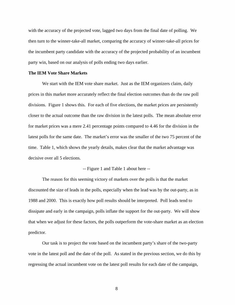
We start with the IEM vote share market. Just as the IEM organizers claim, daily

prices in this market more accurately reflect the final election outcomes than do the raw poll

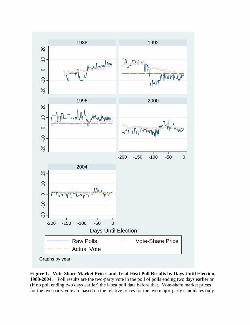
divisions. Figure 1 shows this. For each of five elections, the market prices are persistently

closer to the actual outcome than the raw division in the latest polls. The mean absolute error

for market prices was a mere 2.41 percentage points compared to 4.46 for the division in the

latest polls for the same date. The market’s error was the smaller of the two 75 percent of the

time. Table 1, which shows the yearly details, makes clear that the market advantage was

decisive over all 5 elections.

-- Figure 1 and Table 1 about here --

The reason for this seeming victory of markets over the polls is that the market

discounted the size of leads in the polls, especially when the lead was by the out-party, as in

1988 and 2000. This is exactly how poll results should be interpreted. Poll leads tend to

dissipate and early in the campaign, polls inflate the support for the out-party. We will show

that when we adjust for these factors, the polls outperform the vote-share market as an election

predictor.

Our task is to project the vote based on the incumbent party’s share of the two-party

vote in the latest poll and the date of the poll. As stated in the previous section, we do this by

regressing the actual incumbent vote on the latest poll results for each date of the campaign,

9

using data from previous election years. With 200 dates to cover (from 1 to 200 days before

the election), this is 200 x 5 or 1000 equations. We have separate sets of 200 equations for

each election because each new election expands the moving wall of prior information. For

1988, the information set is all polls 1952-1984. By 2004, the set expands to all polls 1952-

2000.6

-- Figure 2 about here --

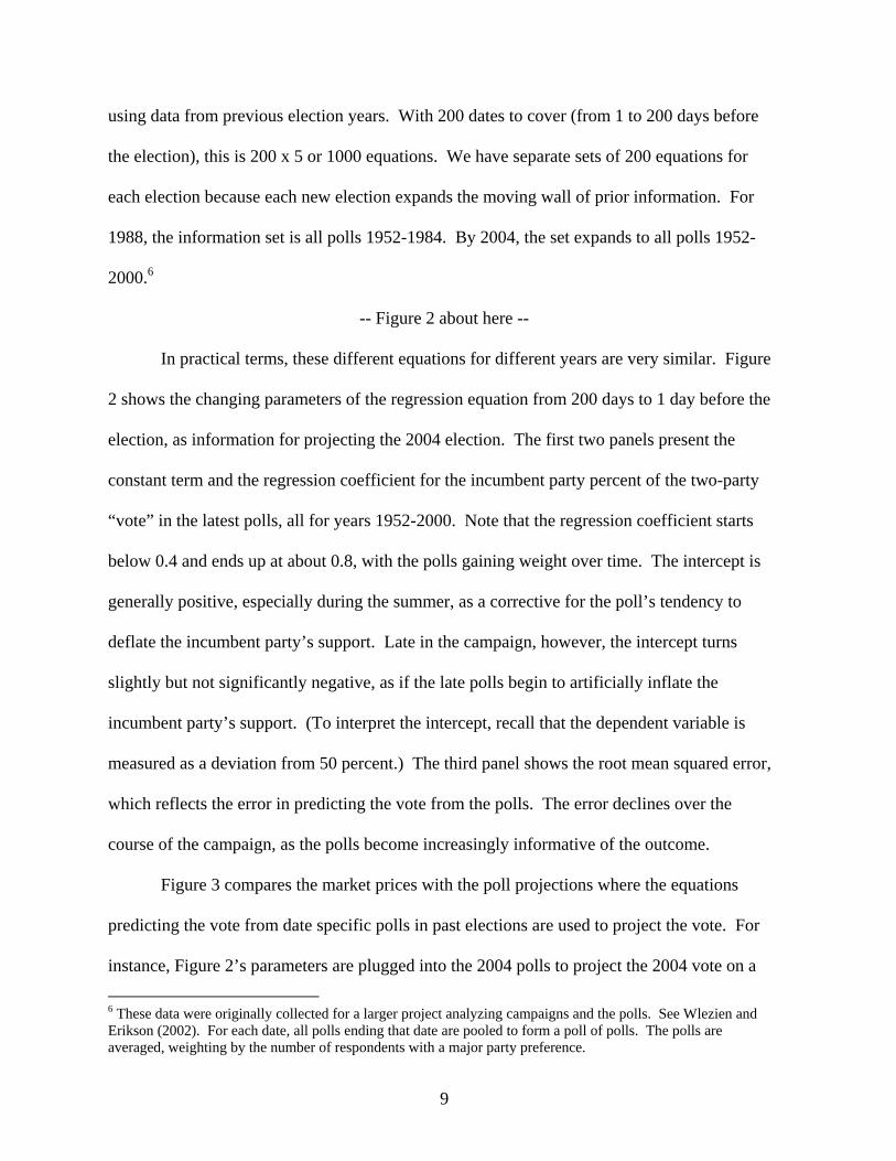
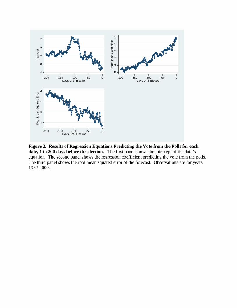
In practical terms, these different equations for different years are very similar. Figure

2 shows the changing parameters of the regression equation from 200 days to 1 day before the

election, as information for projecting the 2004 election. The first two panels present the

constant term and the regression coefficient for the incumbent party percent of the two-party

“vote” in the latest polls, all for years 1952-2000. Note that the regression coefficient starts

below 0.4 and ends up at about 0.8, with the polls gaining weight over time. The intercept is

generally positive, especially during the summer, as a corrective for the poll’s tendency to

deflate the incumbent party’s support. Late in the campaign, however, the intercept turns

slightly but not significantly negative, as if the late polls begin to artificially inflate the

incumbent party’s support. (To interpret the intercept, recall that the dependent variable is

measured as a deviation from 50 percent.) The third panel shows the root mean squared error,

which reflects the error in predicting the vote from the polls. The error declines over the

course of the campaign, as the polls become increasingly informative of the outcome.

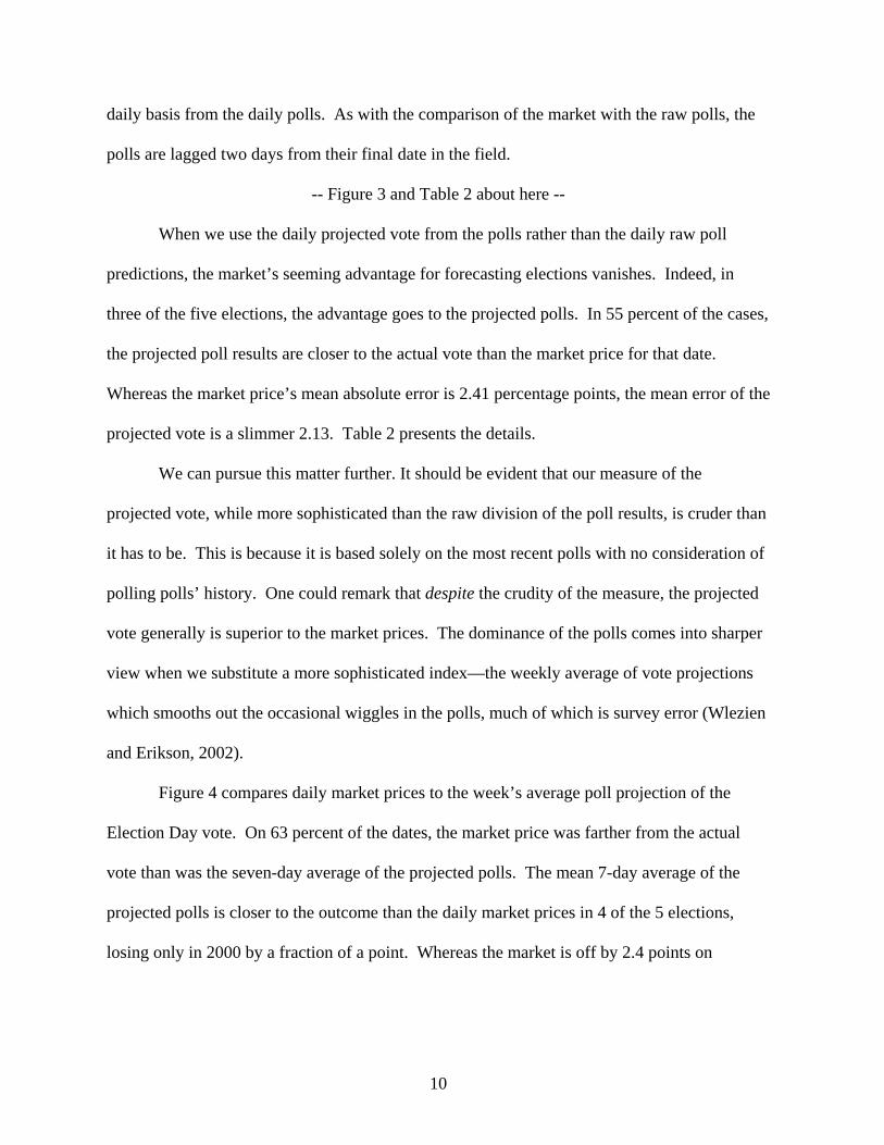
Figure 3 compares the market prices with the poll projections where the equations

predicting the vote from date specific polls in past elections are used to project the vote. For

instance, Figure 2’s parameters are plugged into the 2004 polls to project the 2004 vote on a

6 These data were originally collected for a larger project analyzing campaigns and the polls. See Wlezien and Erikson (2002). For each date, all polls ending that date are pooled to form a poll of polls. The polls are averaged, weighting by the number of respondents with a major party preference.

10

daily basis from the daily polls. As with the comparison of the market with the raw polls, the

polls are lagged two days from their final date in the field.


When we use the daily projected vote from the polls rather than the daily raw poll

predictions, the market’s seeming advantage for forecasting elections vanishes. Indeed, in

three of the five elections, the advantage goes to the projected polls. In 55 percent of the cases,

the projected poll results are closer to the actual vote than the market price for that date.

Whereas the market price’s mean absolute error is 2.41 percentage points, the mean error of the

projected vote is a slimmer 2.13. Table 2 presents the details.

We can pursue this matter further. It should be evident that our measure of the

projected vote, while more sophisticated than the raw division of the poll results, is cruder than

it has to be. This is because it is based solely on the most recent polls with no consideration of

polling polls’ history. One could remark that despite the crudity of the measure, the projected

vote generally is superior to the market prices. The dominance of the polls comes into sharper

view when we substitute a more sophisticated index—the weekly average of vote projections

which smooths out the occasional wiggles in the polls, much of which is survey error (Wlezien

and Erikson, 2002).

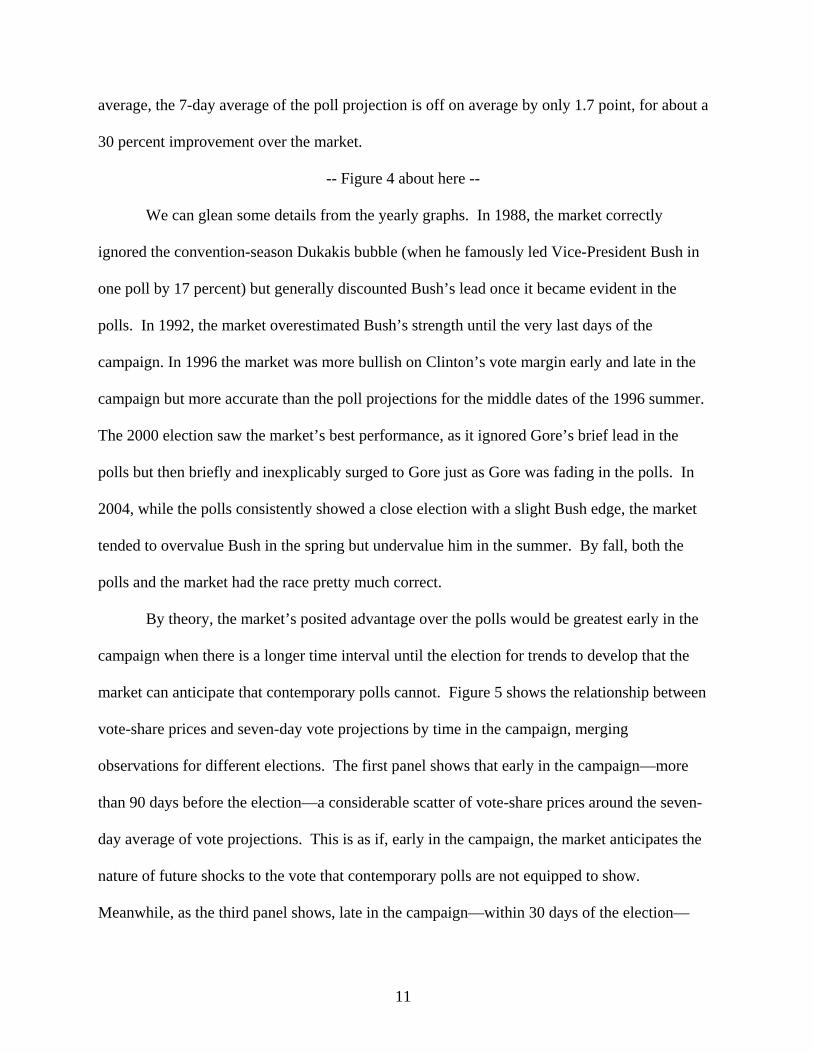
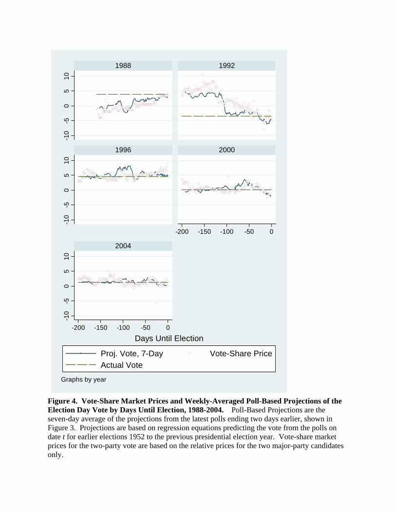
Figure 4 compares daily market prices to the week’s average poll projection of the

Election Day vote. On 63 percent of the dates, the market price was farther from the actual

vote than was the seven-day average of the projected polls. The mean 7-day average of the

projected polls is closer to the outcome than the daily market prices in 4 of the 5 elections,

losing only in 2000 by a fraction of a point. Whereas the market is off by 2.4 points on

11

average, the 7-day average of the poll projection is off on average by only 1.7 point, for about a

30 percent improvement over the market.


We can glean some details from the yearly graphs. In 1988, the market correctly

ignored the convention-season Dukakis bubble (when he famously led Vice-President Bush in

one poll by 17 percent) but generally discounted Bush’s lead once it became evident in the

polls. In 1992, the market overestimated Bush’s strength until the very last days of the

campaign. In 1996 the market was more bullish on Clinton’s vote margin early and late in the

campaign but more accurate than the poll projections for the middle dates of the 1996 summer.

The 2000 election saw the market’s best performance, as it ignored Gore’s brief lead in the

polls but then briefly and inexplicably surged to Gore just as Gore was fading in the polls. In

2004, while the polls consistently showed a close election with a slight Bush edge, the market

tended to overvalue Bush in the spring but undervalue him in the summer. By fall, both the

polls and the market had the race pretty much correct.

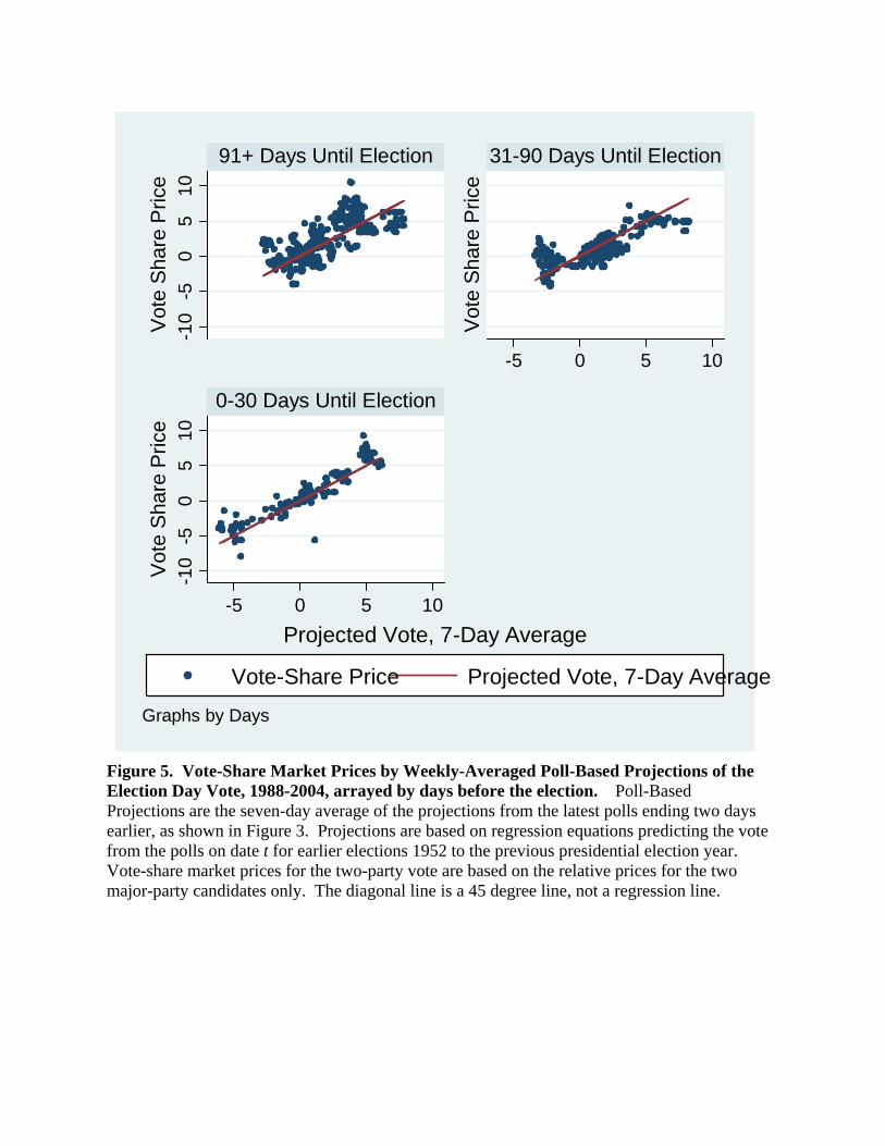
By theory, the market’s posited advantage over the polls would be greatest early in the

campaign when there is a longer time interval until the election for trends to develop that the

market can anticipate that contemporary polls cannot. Figure 5 shows the relationship between

vote-share prices and seven-day vote projections by time in the campaign, merging

observations for different elections. The first panel shows that early in the campaign—more

than 90 days before the election—a considerable scatter of vote-share prices around the seven-

day average of vote projections. This is as if, early in the campaign, the market anticipates the

nature of future shocks to the vote that contemporary polls are not equipped to show.

Meanwhile, as the third panel shows, late in the campaign—within 30 days of the election—

12

the share prices begin to fall in line with vote projections, as if the market tracks the polls now

that there are few shocks to come. Do the market’s departures from the poll projections early in

the campaign signal that the market sees future events that the polls cannot see?7

-- Figures 5 and 6 about here --

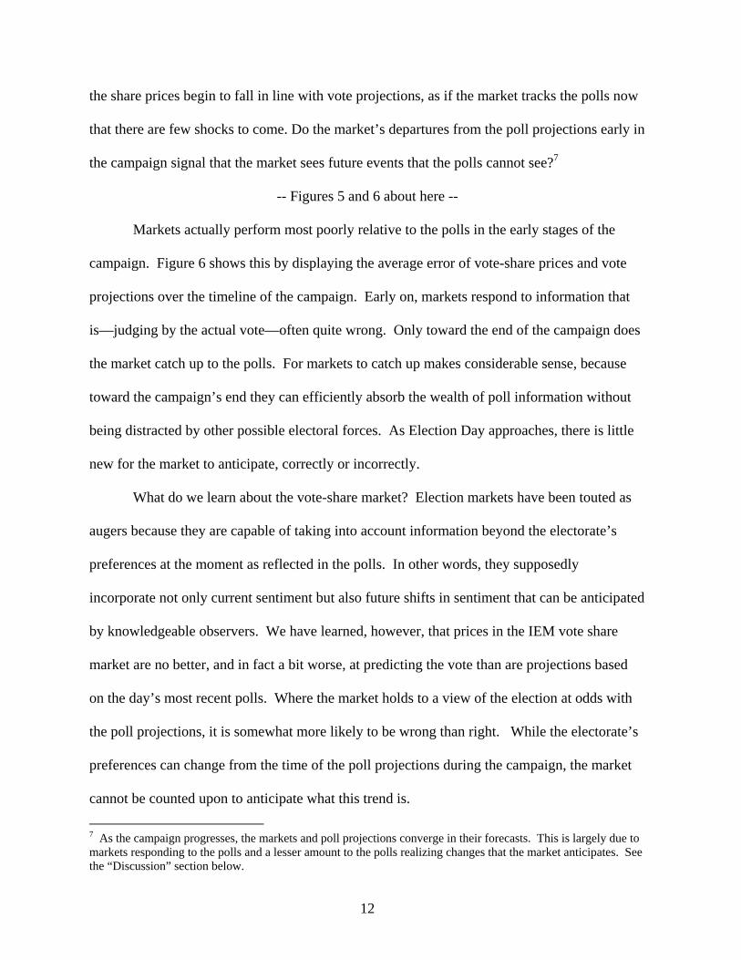
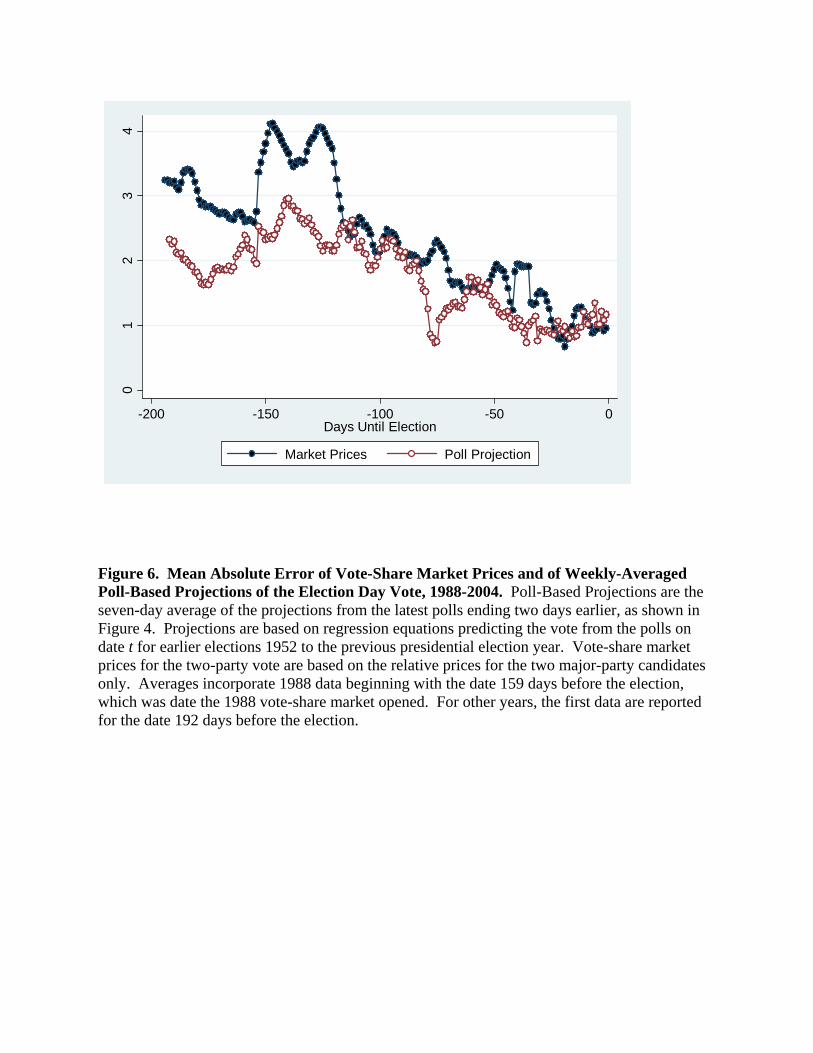
Markets actually perform most poorly relative to the polls in the early stages of the

campaign. Figure 6 shows this by displaying the average error of vote-share prices and vote

projections over the timeline of the campaign. Early on, markets respond to information that

is—judging by the actual vote—often quite wrong. Only toward the end of the campaign does

the market catch up to the polls. For markets to catch up makes considerable sense, because

toward the campaign’s end they can efficiently absorb the wealth of poll information without

being distracted by other possible electoral forces. As Election Day approaches, there is little

new for the market to anticipate, correctly or incorrectly.

What do we learn about the vote-share market? Election markets have been touted as

augers because they are capable of taking into account information beyond the electorate’s

preferences at the moment as reflected in the polls. In other words, they supposedly

incorporate not only current sentiment but also future shifts in sentiment that can be anticipated

by knowledgeable observers. We have learned, however, that prices in the IEM vote share

market are no better, and in fact a bit worse, at predicting the vote than are projections based

on the day’s most recent polls. Where the market holds to a view of the election at odds with

the poll projections, it is somewhat more likely to be wrong than right. While the electorate’s

preferences can change from the time of the poll projections during the campaign, the market

cannot be counted upon to anticipate what this trend is.

7 As the campaign progresses, the markets and poll projections converge in their forecasts. This is largely due to markets responding to the polls and a lesser amount to the polls realizing changes that the market anticipates. See the “Discussion” section below.

13

As a final comment on the vote share market, let us consider the profit one could make

from knowing that savvy projection from the polls are better estimates of the final vote spread

than the market’s prices. Suppose for instance, one set up a robotic trading program to always

buy vote-share stock in the candidate whose poll-based prospects appear better than the market

price. (Suppose also that this market were thick enough that one’s trading actions did not

affect market prices.) Let us say that every day the market is open, one buys one unit of the

candidate who our poll analysis suggests is underpriced. Alas, the profit rate would be only

about 1.4 percent of investment. The meagerness of the profit is due to the conservative nature

of the vote-share market. On average, one purchases a unit of a candidate at a price of about

50 cents (a market expectation of winning half the votes). Considering the average edge of

markets over the polls of about 0.7 points, the expected return for a $0.50 investment is about

$0.507 for a somewhat meager 1.4 percent profit. However, although the rewards from our

market strategy accrue slowly, they should be quite steady. Based on a t-test of over 11 on the

weekly average of the projected poll’s net advantage over the market price—the difference in

absolute errors—the probability of a net loss from our poll-based program trading strategy is

infinitesimally low.

Winner-take-all markets

With candidate shares either paying off at full value or no value on Election Day, the

winner-take-all market offers both greater risk and reward than the vote-share market. The

trader’s challenge is also more difficult in the winner-take-all market: Rather than wager based

on their expectation of the final vote, they must also consider the variance around this

expectation in order to assess the probabilities of a Democratic and Republican victory. Our

14

vote projections include a measure of the variance around the expectation, as shown in the

third panel of Figure 2. Based on the degree of fit by which the date’s regression coefficient

predicts the vote form the polls, one can calculate the forecast error around the point

predictions from the poll projections and in turn, estimate the probability that the candidate’s

margin is greater than zero (that is, 50 percent) and thus wins the popular vote, as per equation

3, above.

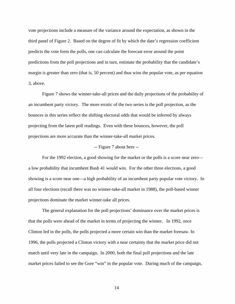
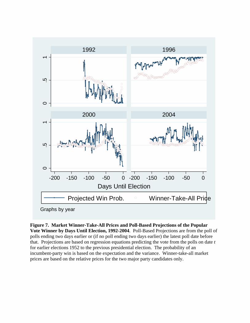
Figure 7 shows the winner-take-all prices and the daily projections of the probability of

an incumbent party victory. The more erratic of the two series is the poll projection, as the

bounces in this series reflect the shifting electoral odds that would be inferred by always

projecting from the latest poll readings. Even with these bounces, however, the poll

projections are more accurate than the winner-take-all market prices.


For the 1992 election, a good showing for the market or the polls is a score near zero—

a low probability that incumbent Bush 41 would win. For the other three elections, a good

showing is a score near one—a high probability of an incumbent party popular vote victory. In

all four elections (recall there was no winner-take-all market in 1988), the poll-based winner

projections dominate the market winner-take all prices.

The general explanation for the poll projections’ dominance over the market prices is

that the polls were ahead of the market in terms of projecting the winner. In 1992, once

Clinton led in the polls, the polls projected a more certain win than the market foresaw. In

1996, the polls projected a Clinton victory with a near certainty that the market price did not

match until very late in the campaign. In 2000, both the final poll projections and the late

market prices failed to see the Gore “win” in the popular vote. During much of the campaign,

15

the poll projection was much more favorable to Gore’s chances than was the market, allowing

the poll projections to score a technical victory in 2000. For much of 2004, the polls

persistently translated Bush 43’s typical slight lead as an incumbent into a far greater

likelihood of victory than the market projected.

The market’s sluggish response to what should have been overwhelming poll numbers

seems due its assigning of a wide variance to the expected vote. Put another way, in addition

to the vote-share market being somewhat behind in estimating the point spread based on

information of the moment (see the discussion of the vote-share market), the winner-take-all

market overestimates the degree to which unexpected events can overtake the market

projection of the point spread. In effect, the market greatly overvalues long-shots.

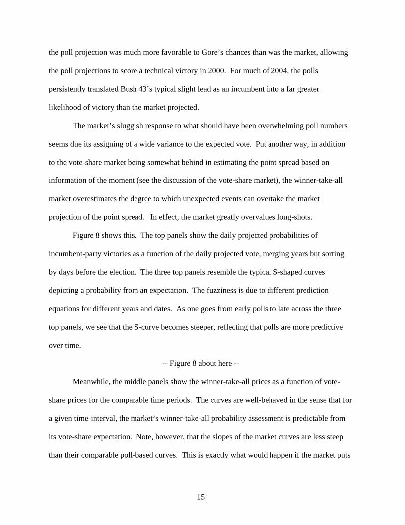
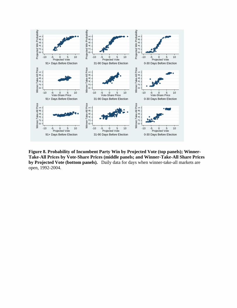
Figure 8 shows this. The top panels show the daily projected probabilities of

incumbent-party victories as a function of the daily projected vote, merging years but sorting

by days before the election. The three top panels resemble the typical S-shaped curves

depicting a probability from an expectation. The fuzziness is due to different prediction

equations for different years and dates. As one goes from early polls to late across the three

top panels, we see that the S-curve becomes steeper, reflecting that polls are more predictive

over time.


Meanwhile, the middle panels show the winner-take-all prices as a function of vote-

share prices for the comparable time periods. The curves are well-behaved in the sense that for

a given time-interval, the market’s winner-take-all probability assessment is predictable from

its vote-share expectation. Note, however, that the slopes of the market curves are less steep

than their comparable poll-based curves. This is exactly what would happen if the market puts

16

a wide variance around its vote-share assessment. The market’s degree of uncertainty about its

own vote-share expectations is greater than the uncertainty about the poll projections. This is

as if the market overestimates the degree to which unanticipated campaign shocks will upend

expectations between then and Election Day.

It follows that the slope of the winner-take-all prices on the poll-based projections

should be even less steep than the slope of the winner-take-all prices on the vote-share prices.

This pattern is born out in the bottom panel. Especially in the early days of the campaign,

when the polls project the verdict to be one-sided, the market is quite uncertain, with variation

in the poll projections having little bearing on winner-take-all prices.

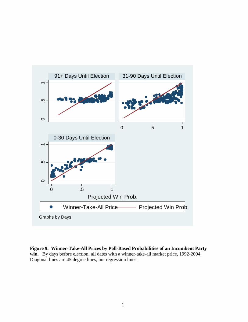
Figure 9 presents the l punch-line of this exercise. It displays the winner-take-all prices

as a function of our objective probabilities based on the vote projections. For the early panel,

based on data 91 days or more before the election, the prices bear virtually no relation to the

probabilities that can be projected from the polls. Indeed, the market cautiously puts the odds

at about 50-50 no matter how certain is the poll projection of the likely outcome. By the

middle dates (31-90 days before the election, the responsiveness of the market to the poll

probability projections improves slightly. By within 30 days of the election, the market moves

almost all the way to the poll projections of the probabilities.


How decisive is this victory of the poll projections over the winner-take-all markets? A

trader who would have picked the undervalued candidate in the market according to the poll

projections would have make the winning choice an astounding 87 percent of the time. As

Table 3 shows, the result is a rout in each year. Overall, a trader who had bought one unit of

17

the undervalued candidate (according to the poll projections) every day would have reaped a

15 percent profit on investment.

Discussion: Where Election Markets Go Wrong (and Right)

So far we have documented that poll projections beat the IEM market. We have

learned the source of the winner-take-all market’s error to be an overestimation of the degree

of surprise still to come during the campaign, so that the market persistently undervalues the

current poll favorite’s chances. The dominance of poll projections over the vote-share market,

while less spectacular, requires explanation. Why did this market fail to do what by theory it is

supposed to do—utilize information beyond the snapshot of current sentiment as revealed in

the polls—to forecast elections accurately?

What moves the vote-share market? Does it respond to recent voter sentiment, as

registered by the polls? Is there any evidence that the vote-share market anticipates actual

shifts in voter preferences? To learn the answers to these questions, we regress both market

prices and the projected vote on lagged prices and lagged vote projections.

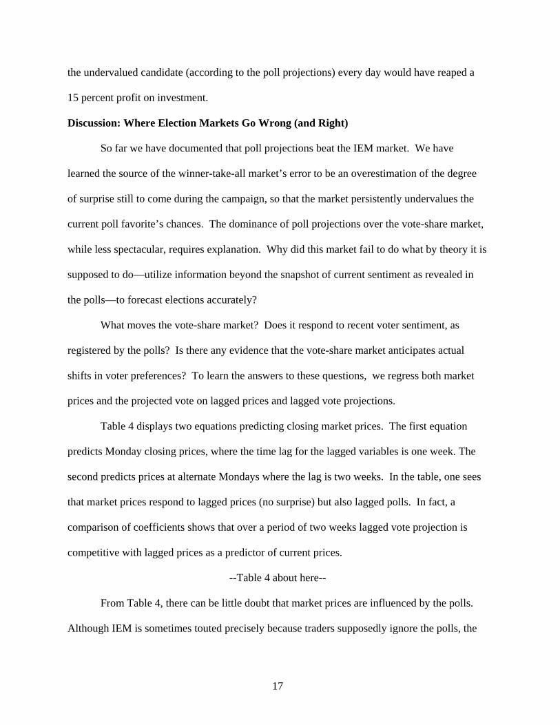
Table 4 displays two equations predicting closing market prices. The first equation

predicts Monday closing prices, where the time lag for the lagged variables is one week. The

second predicts prices at alternate Mondays where the lag is two weeks. In the table, one sees

that market prices respond to lagged prices (no surprise) but also lagged polls. In fact, a

comparison of coefficients shows that over a period of two weeks lagged vote projection is

competitive with lagged prices as a predictor of current prices.

--Table 4 about here--

From Table 4, there can be little doubt that market prices are influenced by the polls.

Although IEM is sometimes touted precisely because traders supposedly ignore the polls, the

18

fact that prices respond to the polls is no indictment of the markets. Market prices should

reflect poll those poll trends that are long-lasting.8

Note for future reference that Table 4 contains no “fixed” (dummy variable) effects for

year. If fixed year effects are added, they are decidedly non-significant and incorporating fixed

effects makes virtually no impact on the key coefficients. That is, election context does not

matter for determining market prices, once one knows the lagged prices and lagged poll-based

vote projections.

Table 5 presents results for parallel models of the weekly average of poll projections as

a function of lagged projections and lagged prices. Just as we did with the price equations of

Table 4, we use weekly and bi-weekly lags.9 Here, in contrast with the price models, we show

equations with and without fixed year effects, because year effects make a difference and offer

clues to the strength and weakness of market prices for electoral forecasting. The attention-

getting feature of Table 5 is the strong showing of lagged market prices as a predictor of poll-

based vote projections. Their strength inspired us to predict vote projections from prices

lagged not only one week or two weeks but even with a lag of four weeks. Thus, Table 5 has

six equations—with three different lag lengths, with and without fixed year effects.

--Table 5 about here--

What do we learn from Table 5? First, there can be little doubt that market prices help

to predict future polls. The proper interpretation of course is not of direct causation, with

markets generating bandwagons in the polls. Rather, we should interpret the “effects” of

8 Polls shift in the short term due to sampling error and to real but short-term change such as so-called convention bounces. What matters for forecasting are long-lasting bumps in voter preferences that survive until Election Day. See Wlezien and Erikson (2002). 9 We “observe” the poll projection weekly averages on Mondays (seven day lag) and alternative Mondays (14 day lag) where the polls’ actual end-date is two days earlier (leaving the field on Saturdays).

19

market prices to be that the election market anticipates change in voter preferences during the

campaign, which becomes reflected in the polls.10

Secondly, we learn that fixed year effects are decidedly significant, and their presence

greatly changes the coefficient for lagged market prices. In each instance, the price effect is

about twice as high with fixed effects. This has the following interpretation. With fixed

effects, price effects are all within-year, so that a strong effect for lagged market prices means

that the stronger “effects” are time-serial: when a candidate’s stock in the market is seemingly

overvalued given the poll numbers, a gain in the polls is likely to follow. The coefficients

without year effects reflect this process as well, but are compromised by persistent year-to-year

distortions in market prices.

Thirdly, when controlling for fixed effects, the “response” of the polls to market prices

increases with the time lag. While the response over one week is impressive, it is even more

impressive over two weeks, when incorporating fixed effects. When lagged over two weeks,

market prices predict the poll-based projected vote slightly better than the lagged projected

vote. When the lag is doubled again to four weeks, in a stunning “victory” market prices

totally dominate the lagged dependent variable as a predictor of poll-based poll projections.

The effect of lagged projections is in fact virtually zero and decidedly non-significant. This is

as if the market does a great job of incorporating both polling information but also information

about what will move the polls over the subsequent four weeks. It seemingly incorporates the

polls so well, that over a four-week horizon, the polls add nothing that the market does not

show.

10 Another way to demonstrate the market’s anticipation of short-term shifts in the projected vote is to regress market price as the dependent variable on lagged price, current poll projection, and future change (first difference) in the poll projection, using either 7 or 14 day lags. In each instance, the future vote shift is positive and significant.

20

Before we climb totally aboard the market bandwagon, however, let us mull a fourth

observation from Table 5—the large year effects. These fixed effects (which are statistically

significant only with lagged prices in the equation11) compensate for systematic error in the

market prices. These “effects” actually represent market distortions—for market prices to

predict poll-based projections, the prices must be adjusted for the market’s persistent tendency

to overestimate or underestimate the incumbent’s vote in the particular year.

This leads to a fifth observation about Table 5. The sizeable year effects grow with the

lag length. Over two weeks they are roughly twice those for one week. Over four weeks they

display further growth, almost doubling once again. By inference, over longer lengths—such

as between early polls and the final vote, they should be larger still. The regular growth of

year effects with lag length is consistent with the market suffering from judgment biases that

persist throughout the campaign. The market distortions from these year-specific persistent

market biases more than offset the market’s ability to discern short-term electoral change

before it registers in the polls.

Finally, consider our sixth and last observation from Table 5. Ideally we would test

markets versus the polls cross-sectionally, with market prices and polls raced as predictors of

election outcomes. With vote-share markets over only five elections, that is not possible.

However, consider that in Table 5, we have a rough substitute in that the dependent variable—

vote projections—measures the state of the election at a particular date in the campaign. The

limitation is that the maximum time gap from polls and market to “vote” is four weeks or less

while the market’s target is the election-day price. But the advantage is a working N. The

11 Although the year effects are not statistically significant when vote projections are modeled solely as a function of lagged projections, they do approach the traditional .05 cutoff level. The p-values are .06, .06, and .11 for lags of 7, 14, and 28 days respectively.

21

appropriate tests are the non-fixed effect equations, particularly over 28 days. We see that in a

cross-sectional battle of predictors, the lagged vote projection still wins handily over lagged

prices. Prices show their worth only when we control for market distortions from year effects.

Unfortunately for forecasting purposes, it is difficult to estimate these yearly distortions in

advance.12

The analysis of this section has provided some insight into why the vote-share prices

predict less well than poll-based information. Whereas the market moves well in the short-

term—in response to polls shifts past and future (anticipated)—it does a poor job of adjusting

its biases about the fundamentals of the elections. While markets may anticipate electoral shifts

(first differences) objectively, it does a poor job of projecting levels of electoral support. The

market holds beliefs about the election’s fundamentals that persist even when they are not true.

This brief excursion can only serve as an introduction to understanding why the vote-

share market does not live up to the claim of greater accuracy than the polls. For example,

beyond persistent biases, another problem with market prices is that they seem prone to the

erratic—seemingly random—movement that could be a sign of a thin market. 13 There may be

some good news though in the fact that the market distortions seem to be on the decline. The

distortions in the first three years of the IEM appear to be larger in magnitude than in 2000 and

2004. Whether this is a real trend, we will have to wait and see.

12 Adjusting for market distortion is not impossible. With sufficient observations over a campaign, one could observe how the polls perform relative to recent market projections. By our analysis, persistent market mistakes should be ignored, while a shift in the first-difference of prices relative to the polls should not be. 13 One might argue that because the market prices display some evidence of autoregressive “error,” prices should be averaged like poll projections. However, if mean market prices provide an improved signal to investors, investors can take further advantage by exploiting short-term variation around the moving average.

22

Conclusion

This paper has tested the claim that the new election stock markets offer superior

predictions of election outcomes than the snapshots from public opinion polls. By our tests,

election markets are not better than the polls for predicting elections. In fact, by a reasonable

as opposed to naïve reading of the polls, the polls dominate the Iowa Electronic market as an

election forecaster. This is true in the sense that a trader in the market can readily profit by

“buying” candidates that informed reading of the polls say are undervalued. Where then do the

markets go wrong? First consider the vote-share market. The histories of market prices show

that traders tend to hold persistent beliefs about the vote division that contradict the polls and

that these persistent beliefs are often wrong. Wrong beliefs get corrected only in the last days

before the election, when the polls are difficult to deny. The winner-take-all market tracks the

vote-share market nicely, but the winner-take-all prices reveal considerable hedging about the

favorite candidate’s chances, as if the market expects more campaign surprises than occur in

reality. The existence of persistent mistakes in the vote-share market compounded by the

degree of uncertainty about the vote-share estimates makes the winner-take-all market a

particularly poor forecasting tool. Based on the experience of the IEM, if the polls show a

candidate to hold a decisive lead but the market is unconvinced, bet on the polls.

One could argue that these negative results are drawn from a limited number of election

years with examples drawn from a toy market with thin volume and limits on trader spending.

With time, the IEM record could improve. And full-blown market like tradesports.com might

in the end achieve an efficiency that so far eludes the Iowa Electronic Market. Interesting

though these possibilities might be, they are not the question. The claim has been made in the

literature that the IEM market dominates the polls, and this claim has wide acceptance. This

23

claim can be considered true only if vote-share prices are naively compared to the polls without

discounting for the likely decline in the size of the polls’ vote margins. Very basic

interpretations of the polls show them to be decisively better at predicting election vote

divisions and—especially—the identity of election winners.

References Berg, Joyce, Forrest Nelson, and Thomas Reitz. 2003. “Accuracy and Forecast Standard Errrors for Prediction Markets.” Working paper. Berge, Joyce E. and Thomas A. Rietz. 2005. “The Iowa Electric Market: Lessons Learned and Answers Yearned.” In Paul Tetlock and Robert Litan (eds). Information Markets: A New Way of Making Decisions in the Public and Private Sector, forthcoming. Berg, Joyce, Robert Forsythe, ,Forrest Nelson, and Thomas Rietz. 2003. “Results from a Dozen Years of Election Futures Market Research.” Working paper. Caldeira, Gregory A. 2004. “Expert Judgment versus Statistical Models: Explanation versus Prediction.” Perspectives on Politics 2:777-780. Campbell, James E. 2000. The American Campaign. College Station: Texas A&M University Press. Kou, Steven and Michael E. Sobel. 2004. “Forecasting the Vote: An Analytical Comparison of Election Markets and Public Opinion Polls.” Political Analysis 12:277-295. Meirowitz, Adam and Joshua A. Tucker. 2004. “Learning from Terrorism Markets.” Perspectives on Politics 2 (June): 331-335. Rohde, Paul W. and Koleman S. Strumpf. 2004. “Historic Presidential Betting Markets.” Journal of Economic Perspectives 18:127-142. Sunstein, Cass. 2004. “Group Judgments: Deliberations, Statistical Means, and Information Markets.” Joint Center: AEI-Brookings Center fro Regulatory Studies Working Paper 04-167. Surowiecki, James. 2004. The Wisdom of Crowds. New York: Doubleday. Wlezien, Christopher and Robert S. Erikson. 2002. “The Timeline of Presidential Election Campaigns.” Journal of Politics 64:969-993. Wolfers, Justin and Eric Zitsewitz. 2004. “Prediction Markets.”Journal of Economic Perspectives, 18.

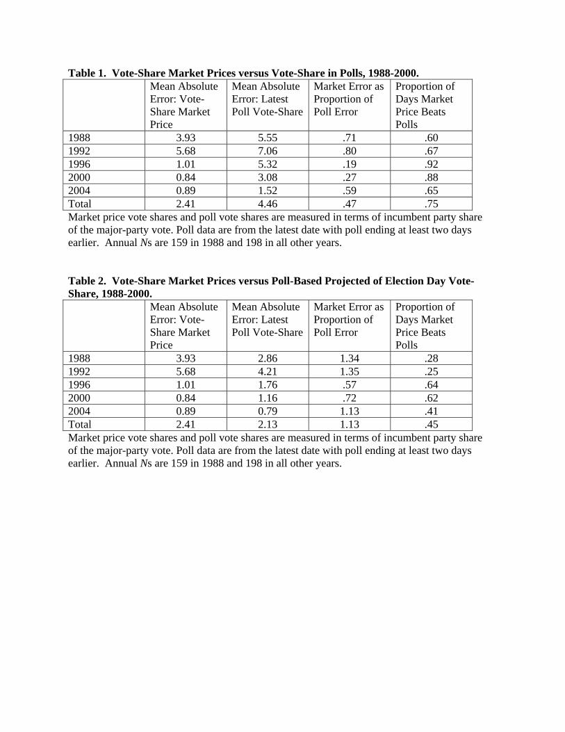
Table 1. Vote-Share Market Prices versus Vote-Share in Polls, 1988-2000.

Mean Absolute Error: Vote-Share Market Price

Mean Absolute Error: Latest Poll Vote-Share

Market Error as Proportion of Poll Error

Proportion of Days Market Price Beats Polls

1988 3.93 5.55 .71 .60 1992 5.68 7.06 .80 .67 1996 1.01 5.32 .19 .92 2000 0.84 3.08 .27 .88 2004 0.89 1.52 .59 .65 Total 2.41 4.46 .47 .75 Market price vote shares and poll vote shares are measured in terms of incumbent party share of the major-party vote. Poll data are from the latest date with poll ending at least two days earlier. Annual Ns are 159 in 1988 and 198 in all other years. Table 2. Vote-Share Market Prices versus Poll-Based Projected of Election Day Vote-Share, 1988-2000.





1988 3.93 2.86 1.34 .28 1992 5.68 4.21 1.35 .25 1996 1.01 1.76 .57 .64 2000 0.84 1.16 .72 .62 2004 0.89 0.79 1.13 .41 Total 2.41 2.13 1.13 .45 Market price vote shares and poll vote shares are measured in terms of incumbent party share of the major-party vote. Poll data are from the latest date with poll ending at least two days earlier. Annual Ns are 159 in 1988 and 198 in all other years.

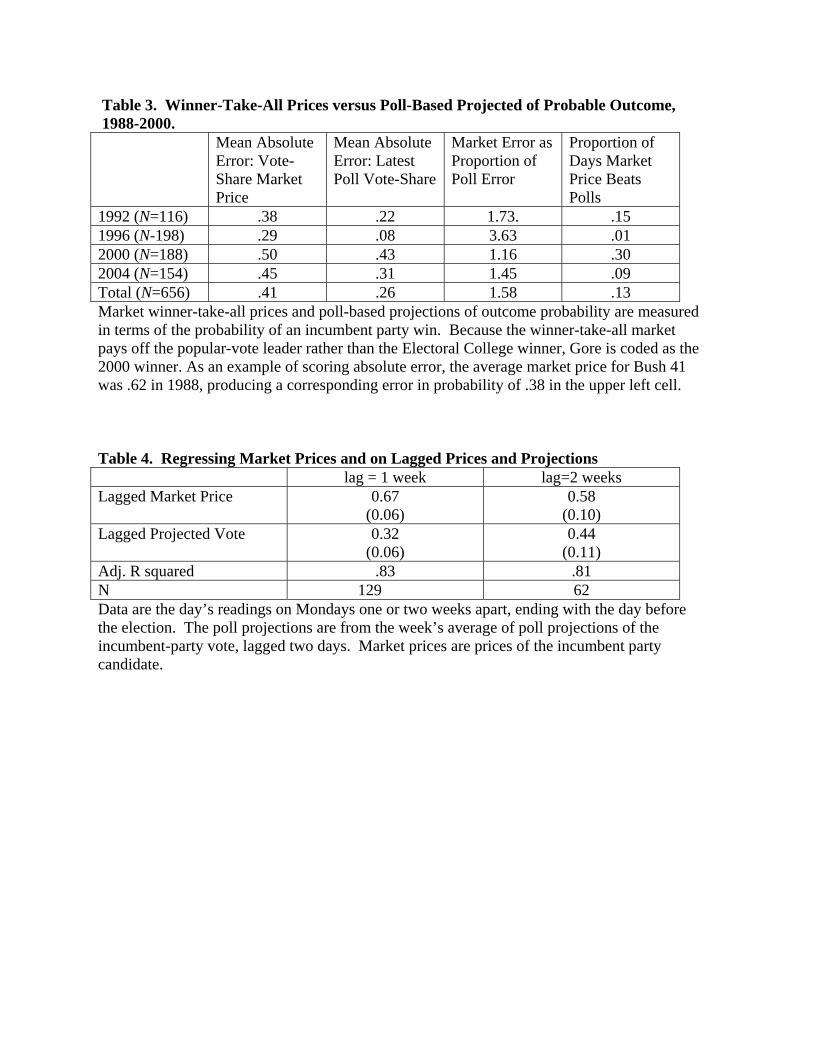
Table 3. Winner-Take-All Prices versus Poll-Based Projected of Probable Outcome, 1988-2000.





1992 (N=116) .38 .22 1.73. .15 1996 (N-198) .29 .08 3.63 .01 2000 (N=188) .50 .43 1.16 .30 2004 (N=154) .45 .31 1.45 .09 Total (N=656) .41 .26 1.58 .13 Market winner-take-all prices and poll-based projections of outcome probability are measured in terms of the probability of an incumbent party win. Because the winner-take-all market pays off the popular-vote leader rather than the Electoral College winner, Gore is coded as the 2000 winner. As an example of scoring absolute error, the average market price for Bush 41 was .62 in 1988, producing a corresponding error in probability of .38 in the upper left cell. Table 4. Regressing Market Prices and on Lagged Prices and Projections lag = 1 week lag=2 weeks Lagged Market Price 0.67

(0.06) 0.58

(0.10) Lagged Projected Vote 0.32

(0.06) 0.44

(0.11) Adj. R squared .83 .81 N 129 62 Data are the day’s readings on Mondays one or two weeks apart, ending with the day before the election. The poll projections are from the week’s average of poll projections of the incumbent-party vote, lagged two days. Market prices are prices of the incumbent party candidate.

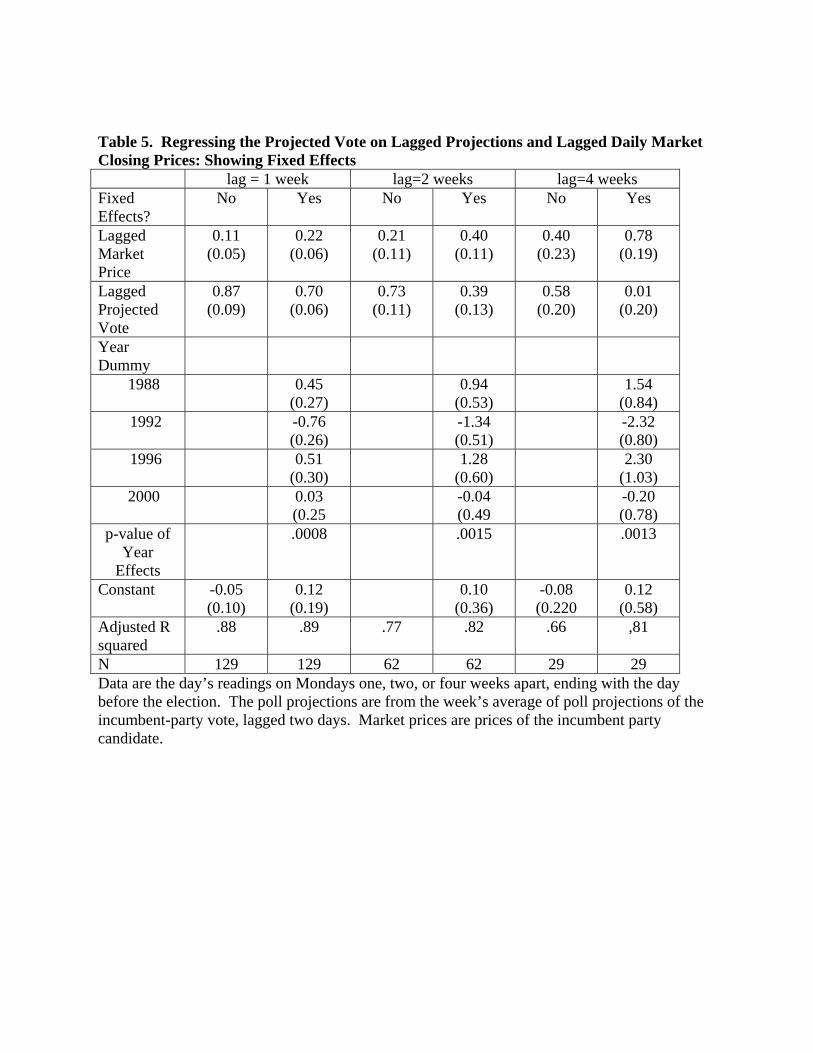
Table 5. Regressing the Projected Vote on Lagged Projections and Lagged Daily Market Closing Prices: Showing Fixed Effects lag = 1 week lag=2 weeks lag=4 weeks Fixed Effects?

No Yes No Yes No Yes

Lagged Market Price

0.11 (0.05)

0.22 (0.06)

0.21 (0.11)

0.40 (0.11)

0.40 (0.23)

0.78 (0.19)

Lagged Projected Vote

0.87 (0.09)

0.70 (0.06)

0.73 (0.11)

0.39 (0.13)

0.58 (0.20)

0.01 (0.20)

Year Dummy

1988 0.45 (0.27)

0.94 (0.53)

1.54 (0.84)

1992 -0.76 (0.26)

-1.34 (0.51)

-2.32 (0.80)

1996 0.51 (0.30)

1.28 (0.60)

2.30 (1.03)

2000 0.03 (0.25

-0.04 (0.49

-0.20 (0.78)

p-value of Year

Effects

.0008 .0015 .0013

Constant -0.05 (0.10)

0.12 (0.19)

0.10 (0.36)

-0.08 (0.220

0.12 (0.58)

Adjusted R squared

.88 .89 .77 .82 .66 ,81

N 129 129 62 62 29 29 Data are the day’s readings on Mondays one, two, or four weeks apart, ending with the day before the election. The poll projections are from the week’s average of poll projections of the incumbent-party vote, lagged two days. Market prices are prices of the incumbent party candidate.

-20

-10

010

20-2

0-1

00

1020

-20

-10

010

20

-200 -150 -100 -50 0

-200 -150 -100 -50 0

1988 1992

1996 2000

2004

Raw Polls Vote-Share PriceActual Vote

Days Until Election

Graphs by year

Figure 1. Vote-Share Market Prices and Trial-Heat Poll Results by Days Until Election, 1988-2004. Poll results are the two-party vote in the poll of polls ending two days earlier or (if no poll ending two days earlier) the latest poll date before that. Vote-share market prices for the two-party vote are based on the relative prices for the two major-party candidates only.

-10

12

3In

terc

ept

-200 -150 -100 -50 0Days Until Election

.3.4

.5.6

.7.8

Reg

ress

ion

Coe

ffici

ent


23

45

Roo

t Mea

n S

quar

ed E

rror


Figure 2. Results of Regression Equations Predicting the Vote from the Polls for each date, 1 to 200 days before the election. The first panel shows the intercept of the date’s equation. The second panel shows the regression coefficient predicting the vote from the polls. The third panel shows the root mean squared error of the forecast. Observations are for years 1952-2000.

-10

-50

510

-10

-50

510

-10

-50

510

-200 -150 -100 -50 0

-200 -150 -100 -50 0

1988 1992

1996 2000

2004

Projected Vote Vote-Share PriceActual Vote

Days Until Election

Graphs by year

Figure 3. Vote-Share Market Prices and Poll-Based Projections of Election Day Two-Party Vote by Days Until Election, 1988-2004. Poll-Based Projections are from the poll of polls ending two days earlier or (if no poll ending two days earlier) the latest poll date before that. Projections are based on regression equations predicting the vote from the polls on date t for earlier elections 1952 to the previous presidential election year. Vote-share market prices for the two-party vote are based on the relative prices for the two major-party candidates only.

-10

-50

510

-10

-50

510

-10

-50

510

-200 -150 -100 -50 0

-200 -150 -100 -50 0

1988 1992

1996 2000

2004

Proj. Vote, 7-Day Vote-Share PriceActual Vote

Days Until Election

Graphs by year

Figure 4. Vote-Share Market Prices and Weekly-Averaged Poll-Based Projections of the Election Day Vote by Days Until Election, 1988-2004. Poll-Based Projections are the seven-day average of the projections from the latest polls ending two days earlier, shown in Figure 3. Projections are based on regression equations predicting the vote from the polls on date t for earlier elections 1952 to the previous presidential election year. Vote-share market prices for the two-party vote are based on the relative prices for the two major-party candidates only.

-10

-50

510

-10

-50

510

-5 0 5 10

-5 0 5 10

Vote

Sha

re P

rice

Vote

Sha

re P

rice

Vot

e S

hare

Pric

e91+ Days Until Election 31-90 Days Until Election

0-30 Days Until Election

Vote-Share Price Projected Vote, 7-Day Average

Projected Vote, 7-Day Average

Graphs by Days

Figure 5. Vote-Share Market Prices by Weekly-Averaged Poll-Based Projections of the Election Day Vote, 1988-2004, arrayed by days before the election. Poll-Based Projections are the seven-day average of the projections from the latest polls ending two days earlier, as shown in Figure 3. Projections are based on regression equations predicting the vote from the polls on date t for earlier elections 1952 to the previous presidential election year. Vote-share market prices for the two-party vote are based on the relative prices for the two major-party candidates only. The diagonal line is a 45 degree line, not a regression line.

01

23

4


Market Prices Poll Projection

Figure 6. Mean Absolute Error of Vote-Share Market Prices and of Weekly-Averaged Poll-Based Projections of the Election Day Vote, 1988-2004. Poll-Based Projections are the seven-day average of the projections from the latest polls ending two days earlier, as shown in Figure 4. Projections are based on regression equations predicting the vote from the polls on date t for earlier elections 1952 to the previous presidential election year. Vote-share market prices for the two-party vote are based on the relative prices for the two major-party candidates only. Averages incorporate 1988 data beginning with the date 159 days before the election, which was date the 1988 vote-share market opened. For other years, the first data are reported for the date 192 days before the election.

0.5

10

.51

-200 -150 -100 -50 0 -200 -150 -100 -50 0

1992 1996

2000 2004

Projected Win Prob. Winner-Take-All Price

Days Until Election

Graphs by year

Figure 7. Market Winner-Take-All Prices and Poll-Based Projections of the Popular Vote Winner by Days Until Election, 1992-2004. Poll-Based Projections are from the poll of polls ending two days earlier or (if no poll ending two days earlier) the latest poll date before that. Projections are based on regression equations predicting the vote from the polls on date t for earlier elections 1952 to the previous presidential election. The probability of an incumbent-party win is based on the expectation and the variance. Winner-take-all market prices are based on the relative prices for the two major party candidates only.

0.2

.4.6

.81

Pro

ject

ed W

in P

roba

bilit

y

-10 -5 0 5 10Projected Vote

91+ Days Before Election

0.2

.4.6

.81

Pro

ject

ed W

in P

roba

bilit

y


31-90 Days Before Election

0.2

.4.6

.81

Pro

ject

ed W

in P

roba

bilit

y



0.2

.4.6

.81

Win

ner-T

ake-

All

Pric

e

-10 -5 0 5 10Vote-Share Price


0.2

.4.6

.81

Win

ner-T

ake-

All

Pric

e



0.2

.4.6

.81

Win

ner-T

ake-

All

Pric

e



0.2

.4.6

.81

Win

ner-T

ake-

All

Pric

e



0.2

.4.6

.81

Win

ner-T

ake-

All

Pric

e


31-90 Days Before Election0

.2.4

.6.8

1W

inne

r-Tak

e-A

ll P

rice



Figure 8. Probability of Incumbent Party Win by Projected Vote (top panels); Winner-Take-All Prices by Vote-Share Prices (middle panels; and Winner-Take-All Share Prices by Projected Vote (bottom panels). Daily data for days when winner-take-all markets are open, 1992-2004.

1

0.5

10

.51

0 .5 1

0 .5 1

91+ Days Until Election 31-90 Days Until Election

0-30 Days Until Election

Winner-Take-All Price Projected Win Prob.

Projected Win Prob.

Graphs by Days

Figure 9. Winner-Take-All Prices by Poll-Based Probabilities of an Incumbent Party win. By days before election, all dates with a winner-take-all market price, 1992-2004. Diagonal lines are 45 degree lines, not regression lines.

are political markets really superior to polls as election ... · are political markets really...

Documents