approximate bayesian recursive estimation

Information Sciences xxx (2014) xxx–xxx

Contents lists available at ScienceDirect

Information Sciences

journal homepage: www.elsevier .com/locate / ins

Approximate Bayesian recursive estimation

http://dx.doi.org/10.1016/j.ins.2014.01.0480020-0255/� 2014 Elsevier Inc. All rights reserved.

⇑ Tel.: +420 266052274.E-mail address: [email protected]

Please cite this article in press as: M. Kárny, Approximate Bayesian recursive estimation, Inform. Sci. (2014), http://dx.doi.org/1j.ins.2014.01.048

Miroslav Kárny ⇑Institute of Information Theory and Automation, Academy of Sciences of the Czech Republic, Pod Vodárenskou vezí 4, 182 08 Prague, Czech Republic

a r t i c l e i n f o a b s t r a c t

Article history:Available online xxxx

Keywords:Approximate parameter estimationBayesian recursive estimationKullback–Leibler divergenceForgetting

Bayesian learning provides a firm theoretical basis of the design and exploitation ofalgorithms in data-streams processing (preprocessing, change detection, hypothesis test-ing, clustering, etc.). Primarily, it relies on a recursive parameter estimation of a firmlybounded complexity. As a rule, it has to approximate the exact posterior probability density(pd), which comprises unreduced information about the estimated parameter. In the recur-sive treatment of the data stream, the latest approximate pd is usually updated using thetreated parametric model and the newest data and then approximated. The fact thatapproximation errors may accumulate over time course is mostly neglected in the estima-tor design and, at most, checked ex post. The paper inspects the estimator design withrespect to the error accumulation and concludes that a sort of forgetting (pd flattening)is an indispensable part of a reliable approximate recursive estimation. The conclusionresults from a Bayesian problem formulation complemented by the minimum Kullback–Leibler divergence principle. Claims of the paper are supported by a straightforward anal-ysis, by elaboration of the proposed estimator to widely applicable parametric models andillustrated numerically.

� 2014 Elsevier Inc. All rights reserved.

1. Introduction

Data-streams processing [2,19] faces many challenges connected with data preprocessing, change detection, hypothesistesting, clustering, prediction, etc. These classical statistical topics [12] are instances of dynamic decision making underuncertainty and incomplete knowledge well-covered by Bayesian paradigm [7]. Its routine use is inhibited by the fact thatthe available formal solutions neglect the inherent need for the recursive (sequential) treatment. The paper counteracts thisneglect with respect to parameter estimation, which forms the core of solutions of the mentioned problems.

The recursive estimation is rarely feasible without an information loss. Mostly, each data updating of estimates onlyapproximates the lossless estimation [9]. Without a care, approximation errors may accumulate to the extent damagingthe estimation quality. Stochastic approximations [5] dominate the analysis inspecting whether a specific estimator suffersfrom this problem or not. The design of estimators avoiding the accumulation is less developed and mostly relies on stochas-tic stability theory [28] limited by a non-trivial choice of an appropriate Lyapunov function.

Both the analysis and design predominantly focus on a point estimation. However, the recursive estimation serving todynamic decision making is to provide a fuller information about the estimated parameter. The Bayesian estimation providesits most complete expression, namely, the posterior probability density of the unknown parameter (pd, Radon–Nikodymderivative with respect to a dominating measure, denoted d�, [33]). This explains the focus of the paper on the Bayesianestimation.

0.1016/

http://dx.doi.org/10.1016/j.ins.2014.01.048

mailto:[email protected]


http://www.sciencedirect.com/science/journal/00200255

http://www.elsevier.com/locate/ins



2 M. Kárny / Information Sciences xxx (2014) xxx–xxx

The inspection of the approximation-errors influence has been neglected within the Bayesian framework. Papers [20–24]represent a significant exception. They characterise the Bayesian approximate recursive estimation without an approxima-tion-errors accumulation. They show that the accumulation is completely avoided if and only if a finite collection of fixedlinear functionals acting on logarithm of the posterior pds are used as a (non-sufficient) statistic. The values of this statisticcan be recursively updated by data and serve as information-bearing constraints for the design of the approximate posteriorpds. This favourable class of statistics is, however, too narrow and excludes too many cases of practical interest. Thus, it isdesirable to inspect an approximate recursive Bayesian estimation allowing non-zero errors caused by the recursive treat-ment while counteracting their accumulation. The paper proposes such an estimator. The proposed solution respects that therecursively stored information about the exact posterior pd (quantifying fully the available information) is inevitably partial.Then, the minimum Kullback–Leibler divergence (KLD, [27]) principle [17,35] is to be used for its completion. Under generalconditions, the completion adds forgetting to a common ‘‘naive’’ approximate recursive estimation, which takes the approx-imate posterior pd as an exact prior pd for the data updating.

The paper primarily aims to attract the research attention to the problem practically faced by any approximate recursivelearning. This determines the relatively abstract presentation way. The excellent anonymous reviewers have served as anencouraging sample of readers who confirmed the presentation efficiency. The suppression of multitude features and tech-nical details of an overall data-streams handling has allowed them to grasp well the essence of the addressed problem and ofits solution. The focus on the problem core also determines the level of proofs’ details. The paper is not fully self-containingin this respect and relies on availability of the complementary information in referred papers. Technically, Section 2 formu-lates the addressed problem. Section 3 provides its solution and indicates that the accumulation of approximation errors iscounteracted. It also guides how to choose the decisive data-dependent forgetting factor. Section 4 specialises the solution toan important class of parametric models and the corresponding feasible approximate posterior pds. An example illustratinggeneral results is in Section 5. Section 6 contains closing remarks.

2. Addressed problem

A parametric model mt ¼ mtðHÞ describes a (modelled) output yt 2 yH1 stimulated by an (external) input ut 2 uH atdiscrete-time moments labelled by t 2 tH ¼ f1;2; . . .g. Data records dt ¼ ðyt ;utÞ are processed sequentially. The parametricmodel mt is a pd of the output yt conditioned on the prior information, on the current input ut , on the past data recordsdt�1; . . . ;d1, and on an unknown parameter H 2 HH. The parameter is also unknown to the input generator. It means that ut

and H are independent when conditioned on dt�1; . . . ;d1, i.e. natural conditions of control [32] are met.Full information about the parameter H at time t � 1 is expressed by the exact posterior pd ft�1 ¼ ft�1ðHÞ ¼

fðHjut; dt�1; . . . ; d1Þ ¼ fðHjdt�1; . . . ; d1Þ (quantifying fully the available information). The Bayes rule Bt updates this pd bythe data record dt . The exact posterior pd evolves as follows

1 xH

scalar-v2 The

conditioargume

Pleasej.ins.2

ft ¼ Bt ½ft�1� () ftðHÞ ¼mtðHÞft�1ðHÞ

gtðytÞ/ mtðHÞft�1ðHÞ; 8 H 2 HH; ð1Þ

gtðytÞ ¼Z

HH

mtðHÞft�1ðHÞdH; ð2Þ

where / denotes equality up to normalisation. The predictive pd gtðyÞ is determined by (2) with the fixed conditionut ; dt�1; . . . ; d1 and an arbitrary output y 2 yH. The parametric model in (1) is treated as likelihood, i.e. as a function of Hfor a fixed inserted data dt ; dt�1; . . . ; d1. The recursion (1) is initiated by a designer-supplied prior pd f0 ¼ f0ðHÞ describingthe available prior information. The updating (1) requires knowledge of the pd ft�1 and information that allows the evalu-ation of the likelihood mtðHÞ; 8 H 2 HH. A j-dimensional statistic wt (called regression vector, j <1), which can be up-dated recursively, is assumed to comprise such an information.

The inspected problem arises when the exact posterior pd ft ¼ ftðHÞ is too complex and has to be replaced by an approx-imate pd pt ¼ ptðHÞ. The pd pt is a projection of ft on a designer-selected set of feasible pds pH. In [8], it was shown that the pdOpt 2 pH approximating optimally the exact posterior pd ft is to minimise the KLD Dðft jjpÞ [27].2

Opt 2 arg minp2pH

DðftjjpÞ ¼ arg minp2pH

ZHH

ftðHÞ lnftðHÞpðHÞ

� �dH: ð3Þ

Since a direct use of (3) with the exact pd ft evolving according to (1) is prevented by the problem definition, the recursiveevaluation without an additional error should evolve the optimal pd Opt (3), i.e. to update recursively the optimal approxima-tion Opt�1 of the exact posterior pd ft�1

Opt�1;mt� �

! Opt : ð4Þ

denotes a set of xs. It is either a non-empty subset of a finite-dimensional real space or a subset of pds acting on the set of unknown parameters. Thealued output is considered without a loss of generality as the multivariate case can always be treated entry-wise [16].KLD, defined in (3) by the integral expression after equality, is conditioned on the data dt ; . . . ; d1. The adopted simplified notation does not mark then explicitly. The KLD has many properties of distance between pds in its argument like non-negativity, equality to zero for almost surely equal

nts, etc. It is, however, asymmetric and does not meet triangle inequality.

cite this article in press as: M. Kárny, Approximate Bayesian recursive estimation, Inform. Sci. (2014), http://dx.doi.org/10.1016/014.01.048



M. Kárny / Information Sciences xxx (2014) xxx–xxx 3

The papers [20–24] mentioned in Introduction have shown that such a construction is possible if and only if the set pH isdelimited by values of a finite collection of linear, time and data invariant, functionals F kðlnðftÞÞ fulfilling F kð1Þ ¼ 0; k ¼1; . . . ;K <1. The exclusion of errors attributed to the recursive treatment excludes commonly used statistics, for instance,(i) the mean and covariance values in unscented approximation [15]; (ii) the likelihood values on a variable, say Monte Carlogenerated, grid [11]; (iii) statistics determining finite Gaussian mixtures with a fixed number of components [3]; (iv) statis-tics yielded by variational Bayes [37]; etc. In other words, the non-commutativity of the Bayes rule (1) and the projection (3)to such classes of pH makes the optimal recursive approximation (4) impossible. Thus, only a non-optimal approximate pdpt 2 pH can be evolved instead of Opt . The ideal recursion (4) is to be replaced by the map recursively updating the pd pt�1

non-optimally approximating the exact posterior pd ft�1

Pleasej.ins.2

pt�1;mtð Þ ! pt : ð5Þ

Such a feasible recursion is mostly constructed in the next naive way, t 2 tH,

Evaluate ~ft ¼ Bt½pt�1�Find ~pt 2 arg min

p2pH

Dð~ftjjpÞ

Set pt ¼ ~pt :

ð6Þ

Often, other proximity measures than the KLD are employed but the use of an approximate pt�1 in the role of the exact pd ft�1

is the common flaw.In summary, a question arises how to construct the map (5) respecting pt�1 – ft�1 or, in other words, how to modify the

recursive approximate estimator (6) so that the approximation-errors accumulation is counteracted.The next auxiliary proposition shows that a difference in prior pds has a tendency to diminish during the data updating.

Proposition 1 (Contractive Nature of the Bayes Rule). Let 8 t 2 tH; ft be the exact posterior pds corresponding to the exact priorpd f0 and pt be the posterior pds initiated by another prior pd p0 such that D0 ¼ Dðf0jjp0Þ <1.

Then, the KLD values Dt ¼ Dðft jjptÞ form super-martingale with respect to r-algebras generated the processed datautþ1; dt ; . . . ; d1. Consequently, Dt converges almost surely to a finite value D1 2 ½0;D0� for t !1.

Proof. Defining the predictive pds gtðyÞ ¼R

HH mtðHÞft�1ðHÞdH and htðyÞ ¼R

HH mtðHÞpt�1ðHÞdH, the key super-martingaleinequality is verified via the following evaluations of the conditional expectation

E½Dt jut ;dt�1; . . . ; d1� ¼Z

yH

gtðyÞZ

HH

ftðHÞ lnftðHÞptðHÞ

� �dH

� �dy

¼Z

yH

ZHH

mtðHÞft�1ðHÞ lnft�1ðHÞpt�1ðHÞ

� �dHdy�

ZyH

gtðyÞ lngtðyÞhtðyÞ

� �dy ¼ Dt�1 � Dðgt jjhtÞ 6 Dt�1:

They use the Bayes rule (1), Fubini theorem [33], the equalityR

yH mtðHÞdy ¼ 1, and non-negativity of the KLD [27]. The finalclaim is the property of any bounded super-martingale [30]. h

A finite number of differences in evaluating of intermediate posterior pds have also tendency diminish. However, theapproximations applied during potentially infinitely repeated data updating may completely spoil the super-martingaleproperty. Then, the accumulated effect can cause the divergence of the KLD Dt for t !1, i.e. the compared pds can becomeasymptotically singular. The possibility of this behaviour formalises the faced problem.

3. Solution

The solution relies on a construction of a sequence of pds’ sets containing the exact posterior pds.

3.1. Circumscribing set

At time t � 1, the approximate pd pt�1 represents the available information about the exact posterior pd ft�1. It differs bothfrom the optimally approximating pd Opt�1 and from the unknown exact posterior pd ft�1. The already cited result [8] impliesthat a pd pt�1 2 pH is an acceptable approximation of the pd ft�1 if there is a finite, ideally small, bt�1 P 0 such thatDðft�1jjpt�1Þ 6 bt�1 <1. Convexity of the functional DðfjjpÞ with respect to the pd f implies convexity of the following setfH

t�1 ¼ fH

pt�1bt�1of pds on HH

fH

t�1 ¼ fH

pt�1bt�1¼ ff : Dðfjjpt�1Þ 6 bt�1 <1g ð7Þ

within which the exact pd ft�1 stays. The expanded notation fH

pt�1bt�1of fH

t�1 stresses its dependence on the given ‘‘centre’’ pt�1

and ‘‘radius’’ bt�1.The following simple proposition shows that the Bayes rule maps the ‘‘ball’’ fH

t�1 on a ball-like set.





Proposition 2 (The Bayes Rule Preserves Convexity). Let a set fH of pds on HH be convex such that for any of its elements f ¼ fðHÞand the considered likelihood m ¼ mðHÞ it holds

RHH mðHÞfðHÞdH > 0. Then, the image B½fH� of fH by the Bayes rule B (1) is convex.

Proof. Let fk 2 fH, k ¼ 1;2. The convexity of fH means that for any a 2 ½0;1� the pd fa ¼ af1 þ ð1� aÞf2 2 fH. Its Bayes image is

Pleasej.ins.2

B½fa� ¼mðaf1 þ ð1� aÞf2Þ

aR

HH mðHÞf1ðHÞdHþ ð1� aÞR

HH mðHÞf2ðHÞdH

¼aR

HH mðHÞf1ðHÞdHaR


HH mðHÞf2ðHÞdH|fflfflfflfflfflfflfflfflfflfflfflfflfflfflfflfflfflfflfflfflfflfflfflfflfflfflfflfflfflfflfflfflfflfflfflfflfflfflfflfflfflfflfflfflfflfflfflffl{zfflfflfflfflfflfflfflfflfflfflfflfflfflfflfflfflfflfflfflfflfflfflfflfflfflfflfflfflfflfflfflfflfflfflfflfflfflfflfflfflfflfflfflfflfflfflfflffl}�

Bðf1Þ þð1� aÞ

RHH mðHÞf2ðHÞdH

aR


HH mðHÞf2ðHÞdH|fflfflfflfflfflfflfflfflfflfflfflfflfflfflfflfflfflfflfflfflfflfflfflfflfflfflfflfflfflfflfflfflfflfflfflfflfflfflfflfflfflfflfflfflfflfflfflffl{zfflfflfflfflfflfflfflfflfflfflfflfflfflfflfflfflfflfflfflfflfflfflfflfflfflfflfflfflfflfflfflfflfflfflfflfflfflfflfflfflfflfflfflfflfflfflfflffl}1��

Bðf2Þ

¼ �B½f1� þ ð1� �ÞB½f2�;

where the coefficient � belongs to the interval [0,1] and the mapping �$ a is bijection. h

The updated exact pd ft ¼ Bt ½ft�1� as well as the pd ~ft ¼ Bt ½pt�1� belong to the convex set Bt ½fH

t�1� ¼ f~f : ~f ¼ Bt ½f�; f 2fH

t�1 ¼ fH

pt�1bt�1g, which is, however, quite complex in the considered generic case. Thus, it is necessary to circumscribe

Bt ½fH

t�1� by the set fH

t ¼ fH

ptbt¼ ff : DðfjjptÞ 6 bt <1g, i.e. by the set of the form (7) for the increased time index.

Proposition 3 (Existence of fH

ptbt). Let the values of the predictive pds gtðyÞ ¼

RHH mtðHÞft�1ðHÞdH; htðyÞ ¼

RHH mtðHÞpt�1ðHÞdH

be positive and finite for y ¼ yt. Let the likelihood mt as well as the ratio

~ft

pt¼ Btðpt�1Þ

a new chosen centre in pH

be essentially bounded with respect to the measure dH. Then a finite bt exists such that fH

t ¼ fH

ptbtcircumscribes Bt ½fH

t�1�.

Proof. The Bayes rule (1), the definition of the KLD (4), the definition of ~ft ¼ Btðpt�1Þ (6), the normalisation of ftðHÞ andsimple manipulations imply

DðftjjptÞ ¼Z

HH

mtðHÞft�1ðHÞgtðytÞ

lnmtðHÞft�1ðHÞgtðytÞptðHÞ

� �dH

¼ 1gtðytÞ

ZHH

mtðHÞft�1ðHÞ lnft�1ðHÞpt�1ðHÞ

� �dHþ

ZHH

mtðHÞft�1ðHÞgtðytÞ

ln~ftðHÞptðHÞ

!dHþ ln

htðytÞgtðytÞ

� �:

After the second equality, the first integral (multiplied by the finite factor 1=gtðytÞ) is bounded as it integrates the product of

the essentially bounded mtðHÞ and of the integrable function ft�1ðHÞ ln ft�1ðHÞpt�1ðHÞ

. The second summand is bounded by the fi-

nite value ln essupHH

~ftðHÞptðHÞ

. The third summand is bounded for positive and finite values of the involved predictive pds. h

The adopted assumptions are probably stronger than necessary but they are verifiable as the realisation of the treateddata record implies positivity of gtðytÞ and other conditions can be inspected analytically.

3.2. Algorithmic construction of the circumscribing set

The construction of the circumscribing set fH

t ¼ fH

ptbtcoincides with the recursive choice of the centre pt and the radius bt .

The Bayes image ~ft ¼ Bt½pt�1� of the centre pt�1 is an obvious candidate for the updated centre. It is generally out of the set pH

of pds of feasible forms so that it cannot be practically used. In accordance with [8], the optimal projection of the pd~ft ¼ Bt ½pt�1� on the set pH of feasible pds offers as a new centre

~pt 2 arg minp2pH

Dð~ft jjpÞ: ð8Þ

Then, it seemingly remains to select the radius bt so that Bt½fH

pt�1bt�1� � fH

~ptbt. A permanent prolongation of this procedure is

impossible as the centre would be updated in the naive way (6) and the error accumulation could cause an unbounded increaseof the radiuses bt of the constructed circumscribing sets for t !1. Thus, a centre pt , which exploits the available informationabout the exact pd ft in a better way, is to be searched for.

A (generally iterative) search for a better centre simplifies substantially if the set of feasible pds pH is closed with respectto taking geometric mean of its elements, if it is log-convex set. Further on, the log-convexity of pH is assumed without a sub-stantial loss of applicability.

The axiomatically justified minimum KLD principle [35] recommends to replace the unknown, partially specified, exactpd ft by a pd fc with the smallest KLD on a pd representing the information before processing the information contained in





the pd ~pt 2 pH (8). The non-updated pd pt�1 is the available descriptor of such a (vague) information. The pd fc is searched inthe trial circumscribing set fH

~ptc ¼ ff : Dðfjj~ptÞ 6 cg parameterised by c 2 ½0;1Þ. The new centre pc is then found as the projec-

tion of fc on the set of feasible pds pH. Then, the trial radius c is chosen so that the radius bt guaranteeing circumscriptionBtðfH

t�1Þ � fH

pcbtis the smallest one. Formally,

Pleasej.ins.2

fc 2 arg minff:Dðfjj~ptÞ6cg

Dðfjjpt�1Þ ð9Þ

pc 2 arg minp2pH

DðfcjjpÞ ð10Þ

ðbt; ctÞ 2 arg minðb;cÞsuch thatffH

pcb�BtðfH

t�1Þgb ð11Þ

pt ¼ pct:

Proposition 4 (The Optimal Centre). Let the set pH of approximate pds be log-convex. Then, the fc solving (9) is in pH. For a giventrial radius c, the solution of (9) and (10) pc ¼ fc has the form of stabilised forgetting [26] determined by a forgetting factorkc 2 ½0;1�

pc ¼ pkc ¼~p

kct p

1�kct�1R

HH ~pkct p

1�kct�1 dH

¼ ~pkct p

1�kct�1

LðkcÞð12Þ

kc ¼ 0 if Dðpt�1jj~ptÞ < ckc solves Dðpcjj~ptÞ ¼ c otherwise:

Proof. The Kuhn–Tucker optimality conditions [14] and the KLD property DðfjjgÞ ¼ 0() f ¼ g dH-almost surely provide thesolution of the task (9). Its form and log-convexity of the set pH imply that fc 2 pH and the nearest pc 2 pH (10) coincides withit. h

The radiuses ðbt ; ctÞ guaranteeing that fH

pctbt

circumscribes the set BtðfH

t�1Þ, i.e. the solution of (11), depend on the chosentrial centre ~pt (8), see (12). The found pd pct

offers itself as a better centre. Under the adopted log-convexity of the set of fea-sible pds pH, the replacement of the centre ~pt by pct

preserves the form (12) of pctand no improvement of bt can be gained.

Thus, an iterative search is avoided.To find the best radiuses ðbt ; ctÞ (11) either analytically or numerically is hard and the mapping of ct on the forgetting

factor kctis also complex. Instead, kt 2 ½0;1� approximately minimising the expectation of the KLD dðft; kÞ ¼ Dðft jjpkÞ, see

(12), is searched for. The following proposition prepares the search and shows that the forgetting has indeed the potentialto counteract the approximation-errors accumulation.

Proposition 5 (Forgotten Probability Density Approximates Better). To any pd f such that Dðfjj~ptÞ <1;Dðfjjpt�1Þ <1, there iskt ¼ ktðfÞ 2 ½0;1� such that Dðfjjpkt

Þ 6 Dðfjj~ptÞ.

Proof. The definitions of the KLD and the pd pk (12) give for any k 2 ½0;1�

dðf; kÞ ¼ DðfjjpkÞ ¼ kDðfjj~ptÞ þ ð1� kÞDðfjjpt�1Þ þ lnðLðkÞÞ:

The definition (12) of the pd pk also implies that pk¼1 ¼ ~pt and pk¼0 ¼ pt�1. Denoting

Rt ¼pk¼1

pk¼0¼ ~pt

pt�1; ð13Þ

derivatives of the function dðf; kÞ get the forms

@dðf; kÞ@k

¼ Dðfjj~ptÞ � Dðfjjpt�1Þ þZ

HH

pkðHÞ ln RtðHÞð ÞdH ð14Þ

@2dðf; kÞ@k2 ¼

ZHH

pkðHÞln2

RtðHÞð ÞdH�Z

HH

pkðHÞ ln RtðHÞð ÞdH� �2

:

The second derivative is the positive variance of ln RtðHÞð Þ with respect to the pd pkðHÞ. Thus, dðf; kÞ is a convex function ofk 2 ½0;1� and reaches its minimum within this closed interval. h

Remarks.

� The necessary condition @dðf;kÞ@k ¼ 0 for selecting the forgetting factor kt ¼ ktðfÞ minimising dðf; kÞ ¼ DðfjjpkÞ has the appeal-

ing form, cf. (13) and (14),





Pleasej.ins.2

ZHH

fðHÞ lnðRtðHÞÞdH ¼Z

HH

pktðHÞ lnðRtðHÞÞdH; ð15Þ

if the extreme is in (0,1). Otherwise, kt 2 f0;1g if no kt solving (15) exists.� The inequality claimed by Proposition 5 cannot be improved. It is trivially met for kt ¼ 1 corresponding to the ‘‘naive’’

approximate learning step. The illustrative example, Section 5, indicates that it often – but not always – happens. Asymp-totically, when the approximate posterior concentrates around the optimal projection of the almost surely convergingexact posterior pd, the optimality of kt ¼ 1 is even desirable.

The exact posterior pd ft is unknown so that the optimal kt ¼ ktðftÞminimising dðft ; kÞ cannot be constructed. Proposition1 shows that the pd ~ft ¼ Btðpt�1Þ is expected to be nearer to the unknown exact pd ft than the approximate pd pt�1 to theexact pd ft�1. Also, Proposition 3 guarantees that Dðfjj~ptÞ <1;Dðfjjpt�1Þ <1 for f 2 f~ft ; ftg. As the left-hand side of (15) de-pends linearly on the considered pd f, it can be expected that the use f ¼ ~ft instead of f ¼ ft will lead to ktð~ftÞ, which makesDðft jjpktð~ft ÞÞ ¼ dðft ; ktð~ftÞÞ < dðft ; k ¼ 1Þ ¼ Dðft jj~ptÞ. Thus, it is reasonable to use kt ¼ ktð~ftÞ instead of the inaccessible ktðftÞ. Thisis the only heuristic step in designing the final recursive estimation applicable 8t 2 tH.

Algorithm 1. Approximate Recursive Bayesian Estimation

~

ci01

Evaluate ft ¼ Bt ½pt�1� / mtpt�1

Find ~pt 2 argminp2pH

Dð~ft jjpÞ

Define pk / ~pkt p

1�kt�1 ; for k 2 ½0;1�; and Rt ¼

~pt

pt�1

Find kt 2 ½0;1�solv ing

ð16Þ

Z Z
HH
~ftðHÞ lnðRtðHÞÞdH ¼HH

pktðHÞ lnðRtðHÞÞdH ð�Þ

if no solution of ð�Þ exists set kt ¼0 if

RHH

~ftðHÞ lnðRtðHÞÞdH � 01 otherwise

(

Forget pt ¼ pkt:

Remarks.

� Algorithm 1 rectifies the estimator (6) by complementing it by a stabilised forgetting applied to the naive approximate pd~pt , while using the pd pt�1 as the needed alternative.� Algorithm 1 reduces to the naive estimator (6) for kt ¼ 1. It happens whenever no projection is needed after data updat-

ing, whenever ~ft ¼ ~pt 2 pH. Thus, it does not spoil the feasible optimal recursion. This smooth transition to the exact recur-sive estimation is an intuitively desirable property.� Similar ‘‘flattening’’ techniques counteracting errors’ accumulation are already used, for instance, within applications of

Monte Carlo methods for a recursive parameter estimation [31]. The proposed treatment formally supports the need for atechnique of this type and recommends its form (12) without adding a new ‘‘tuning knob’’.

4. Dynamic regression model with an arbitrary noise

The widely applicable class of dynamic regression parametric models with an external inputs (briefly regression models)with an arbitrary noise is considered here. It: (i) is useful per se; (ii) illustrates the respective steps of the general estimationalgorithm; (iii) indicates a mild increase of the computational complexity needed for the proposed counteracting of the erroraccumulation. Algorithm 1 is tailored to this common parametric model, which arises from the following functional expan-sion of the conditional expectation

yt ¼ E½yt jut ;dt�1; . . . ; d1;H� þffiffiffirp

et ¼ h0wt þffiffiffirp

et;0 is transposition: ð17Þ

Such an expansion is often possible at least locally. The noiseffiffiffirp

et as the difference between the output and its conditionalexpectation has the conditional expectation equal to zero. As such, it is uncorrelated over time and uncorrelated with data inthe condition. The j-dimensional regression vector wt ;j <1, is supposed to be recursively updatable. This makes the recur-sive updating of the data vector Ut consisting of the output yt and of the regression vector wt possible. The unknown param-eter H ¼ ðh; rÞ includes the regression coefficients h and a scaling parameter r > 0 used in a pd 1ffiffi

rp g e; rð Þ defining the distribution

of the scaled noise e. With it, the parametric regression model gets the form

te this article in press as: M. Kárny, Approximate Bayesian recursive estimation, Inform. Sci. (2014), http://dx.doi.org/10.1016/4.01.048




Pleasej.ins.2

mtðHÞ ¼1ffiffiffirp g

½1;�h0�ffiffiffirp Ut; r

� �¼ 1ffiffiffi

rp g g0Ut; rð Þ; g0 ¼ g0ðh; rÞ ¼ ½1;�h0�ffiffiffi

rp : ð18Þ

When delimiting known properties of the noise, its distribution g is obtained by the minimum KLD principle. For instance,assuming that r is a finite noise variance and reducing the minimum KLD principle to maximum entropy principle, the allo-

cated noise distribution is Gaussian. In the Gaussian case with the pd gðe; rÞ ¼ ð2pÞ�0:5 exp � e2

2

h i, the regression model has

the Gauss-inverse-Wishart (GiW, [32]) as the conjugated prior

ptðHÞ ¼ pLt ;mtðh; rÞ ¼ r�0:5ðmtþjþ2Þ exp½�0:5g0L0tLtg�

JðLt ; mtÞ; H ¼ ðh; rÞ; ð19Þ

where Lt is lower triangular matrix with positive diagonal (symbolically, Lt > 0; it is Choleski square root of the extendedinformation matrix), scalar mt > 0 and j is the length of the regression vector wt , which equals to the number of regressioncoefficients.

For the Gaussian regression model, this pd preserves its form during estimation and its use converts the data updating ofthe posterior pds into the algebraic updating

L0tLt ¼ L0t�1Lt�1 þUtU0t; mt ¼ mt�1 þ 1: ð20Þ

The recursion starts from the chosen prior values L0 > 0 and m0 > 0.The GiW pds have a chance to approximate well the exact posterior pds even for non-Gaussian regression models. This

follows from the fact that the exact posterior pds quickly concentrate on a narrow support in HH ¼ ðhH; rHÞ. It happens undergeneral conditions [6] allowing the extension of the classical large-deviation theorem [34] to externally stimulated dynamicsystems.

4.1. Specialisation of Algorithm 1

The specialisation of Algorithm 1 exploits the following elementary properties of the GiW pd, proved for instance in [16].They are expressed in terms of the following splitting of the extended information matrix Vt ¼ L0tLt

Vt ¼Vt;y V 0t;yw

Vt;yw Vt;w

" #¼

L2y þ L0ywLyw L0ywLw

L0wLyw L0wLw

" #> 0: ð21Þ

There, Vt;y; Lt;y are scalars. The time index, separated by semicolon, is dropped whenever its occurrence brings noinformation.

Proposition 6 (Some Properties of GiW Probability Density). Let us consider GiW pds pLt�1 ;mt�1; peLt ;~mt

with JðLt�1; mt�1Þ <1 andJðeLt ; ~mtÞ <1. Then, the pd pk / ~pk

t p1�kt�1 , given by k 2 ½0;1�, is the pd pLk;mk

with

L0kLk ¼ k eL0t ; ffiffiffiffiffiffiffiffiffiffiffiffiffiffiffiffik�1 � 1

pL0t�1

h i eL0t; ffiffiffiffiffiffiffiffiffiffiffiffiffiffiffiffik�1 � 1

pL0t�1

h i0; mk ¼ k~mt þ ð1� kÞmt�1: ð22Þ

For a GiW pd given by statistic values Lt > 0; mt > 0 the normalisation factor JðLt ; mtÞ in (19) is finite. Consequently, JðLk; mkÞ <1for Lt�1 > 0; mt�1 > 0. The set pH of GiW pds (19), serving as approximate feasible posterior pds, is log-convex set and the construc-tion from Section 3.2 is directly applicable.

It holds

JðL; mÞ ¼ p0:5jCð0:5mÞð0:5KÞ�0:5mjCj0:5; E½hjL; m� ¼ h; E½r�1jL; m� ¼ 1r¼ m

K

E½lnðrÞjL; m� ¼ lnð0:5KÞ �Wð0:5mÞ; E½gg0jL; m� ¼ 1r

1 h0

h hh0 þ rC

" #:

There psi function WðxÞ ¼ @CðxÞ@x ;CðxÞ ¼

R10 zx�1 expð�zÞdz <1 for x > 0, [1], and entities known from least squares estimation

method are used

C ¼ V�1w ¼ L�1

w L�1w

0; K ¼ Vy � V 0ywV�1

w Vyw ¼ L2y ; h ¼ L�1

w Lyw: ð23Þ
Recalling that the GiW pds (19) form the assumed set pH of feasible approximate pds, the specialisation of Algorithm 1
starts with the application of the Bayes rule to the pd pt�1 ¼ pLt�1 ;mt�1and likelihood of the form (18)

~ftðh; rÞ / gðg0Ut ; rÞpLt�1 ;mt�1þ1ðh; rÞ: ð24Þ

The association of the factor 1ffiffirp with the prior pd pLt�1 ;mt�1

makes the considered likelihood essentially bounded in generic case.The KLD definition, the form of the approximating GiW pd and (24) imply that the approximate pd ~pt ¼ peLt ;~mt

minimisingthe KLD Dð~ft jjpÞ is determined by the statistic values eLt ; ~mt





Pleasej.ins.2

eLt ; ~mt 2 argminL;m

f�2ln jLwj þ2lnðCð0:5mÞÞ� m lnð0:5L2yÞþ ðmþjþ2Þat þ tr½Bt;yðL2

y þ L0ywLywÞþ2B0t;ywL0wLyw� þ tr½Bt;wL0wLw�g

at ¼ZðhH ;rHÞ

lnðrÞgðg0Ut ;rÞpLt�1 ;mt�1þ1ðh;rÞR

ðhH ;rHÞ gðg0Ut;rÞpLt�1 ;mt�1þ1ðh;rÞdhdrdhdr

Bt ¼ZðhH ;rHÞ

gg0gðg0Ut; rÞpLt�1 ;mt�1þ1ðh; rÞR

ðhH ;rHÞRðhH ;rHÞ gðg0Ut ; rÞpLt�1 ;mt�1þ1ðh; rÞdhdr

dhdr ¼Bt;y B0t;yw

Bt;yw Bt;w

" #¼

Ut;y 0Ut;yw U0t;w

" #Ut;y U0t;yw

0 Ut;w

" #: ð25Þ

The scalar at and the positive definite matrix Bt can be found efficiently by Monte Carlo sampling from the GiW pdpLt�1 ;mt�1þ1ðh; rÞ. The upper-triangular Choleski factors Ut of Bt splits similarly as Vt (21).

Proposition 7 (The Best Projection on a GiW Probability Density). The GiW minimiser peLt ;~mtðh; rÞ of Dð~ft jjpL;mÞ for ~ftðh; rÞ, see (24),

is given by

eV�1t;w ¼ eCt ¼ Bt;w () eLt;w ¼ U�1

t;w

0eV t;yw ¼ �B�1

t;yeV t;wBt;yw () eLt;yw ¼ �U�1

t;y U�1t;w

0Ut;yw () ~ht ¼ �U�1

t;y Ut;yw

eV t;y ¼~mt

Bt;yþ eV 0t;yw

eV�1t;weV t;yw () ~Kt ¼

~mt

Bt;y¼ 1

~rt

() eLt;y ¼ffiffiffiffiffi~mt

pUt;y

ln 0:5~mtð Þ �Wð0:5~mtÞ ¼ at þ lnðBt;yÞ; Bt;y ¼ U2t;y; ð26Þ

where W function and the least-squares entities (23), for eV t ¼ eL0teLt, are used.

Proof. The proof exploits the necessary conditions for extreme, the matrix identities @ lnðjCjÞ@C ¼ C�1, @trðCDÞ

@C ¼ D0 and simplemanipulations. h

The Eq. (26) for the positive scalar s ¼ 0:5~mt is the only one to be solved iteratively. The following proposition shows thatthe solution exists. It indicates that no problems should be encountered in a numerical solution.

Proposition 8 (The Solution of (26)). The solution of (26) exists.

Proof. The right-hand side of the inspected equation has the form at þ lnðBt;yÞ ¼ �E½lnðr�1Þ� þ lnðE½r�1�ÞP 0, cf. (25). Thenon-negativity of this expression follows from Jensen inequality [33] applied either to the exact expectation or its MonteCarlo approximation. The same inequality also allows the bounding of the left-hand side

lnðsÞ �WðsÞ ¼ lnðsÞ �@ ln

R10 zs�1 expð�zÞdz

� �@s

¼ lnðsÞ �Z 1

0lnðzÞ zs�1 expð�zÞR1

0 zs�1 expð�zÞdzdz P lnðsÞ � ln

Cðsþ 1ÞCðsÞ

� �¼ 0;

where the equality Cðsþ 1Þ ¼ sCðsÞ, [1], is used.Moreover, �WðsÞ ¼ 1

sþ fðsÞ, for s! 0þ, where fðsÞ is a bounded function [1]. Thus, the left-hand sidelnðsÞ �WðsÞ ¼ 1

s ðs lnðsÞ þ 1Þ þ fðsÞ increases to infinity for s! 0þ. This together with the continuous dependence of thisfunction on s implies the claim. h

Having the projection p~Lt ;~mt, it remains to find the forgetting factor kt meeting (�) in (16).

Proposition 9 (Forgetting factor). Let us consider the approximate GiW pd (19) and denote

Dm ¼ mt�1 � ~mt; DV ¼ Vt�1 � eV t: ð27Þ

Then, the forgetting factor kt 2 ½0;1� minimising dð~ft ; kÞ ¼ Dð~ftjjpLk ;mkÞ is

(i) either a unique solution of the equation

Dmat þ tr U0tUtDV� �

ð28Þ

" # !
¼ Dm½lnð0:5KkÞ �Wð0:5mkÞ� þ tr
1rk

1 h0khk hkh0k þ rkCk

DV





Pleasej.ins.2

¼ Dm½lnð0:5L2ykÞ �Wð0:5mkÞ� þ tr L�1

k L�1k

0DV

; ð29Þ

where at;Bt ¼ U0tUt are defined in (25). The used least squares entities correspond to the extended information matrix Vk ¼ L0kLk,see (22) also defining mk,

(ii) or equals 0 for (cf. (23))

Dmat þ tr U0tUtDV� �

þ 2 lnJðLt�1; mt�1Þ

JðeLt ; ~mtÞ

!6 0 ð30Þ

(iii) otherwise equals 1.

Proof. The statement is specialisation of the general results and the equation (�) in (16). In the considered case,

2 lnðRtðh; rÞÞ ¼ Dm lnðrÞ þ tr gg0DVð Þ þ 2 lnJðLt�1; mt�1Þ

JðeLt; ~mtÞ

!|fflfflfflfflfflfflfflfflfflfflfflfflfflfflfflffl{zfflfflfflfflfflfflfflfflfflfflfflfflfflfflfflffl}

x

ð31Þ

The left-hand side (lht) of the inspected equation (�) gets the form

lht ¼ Dmat þ tr U0tUtDV� �

þx

The right-hand side (rht) gets the analytical form

rht ¼ DmEk½lnðrÞ� þ tr Ek gg0½ �DVð Þ þx;

where Ek is expectation with respect to the inspected pLk ;mk. The explicit formulae for the needed moments are in Proposition

6 and then it remains to set lht ¼ rht . If the solution does not exist then k ¼ 0 is minimiser if Dð~ftjjpt�1Þ 6 Dð~ft jj~ptÞ, whichtranslates into the condition (30). h

This concludes specialisation of Algorithm 1 for the regression model (18) and the GiW class of approximate pds (19).

Algorithm 2. Approximate Recursive Bayesian Estimator for (18 and 19)

Initial phase

� Specify the regression model by specifying the modelled output y 2 yH, structure of the regression vector w and thepd g of the noise.� Set t ¼ 0 and specify the values of the prior statistic Lt; mt .� Select parameters controlling evaluations, i.e. the number of Monte Carlo samples of H ¼ ðh; rÞ and a precision used

in solving equations for mt and kt .Recursive phase, running for t 2 tH,1. Increase time counter.2. Evaluate at ;Ut in (25) for the processed data vector U0t ¼ ½yt;w

0t�.

3. Evaluate the statistic values eLt ; ~mt according to (26).4. Determine the forgetting factor kt as specified in Proposition 9.5. Set L0tLt ¼ kt

eL0teLt þ ð1� ktÞL0t�1Lt�1; mt ¼ kt~mt þ ð1� ktÞmt�1.

In a generic case, Step 2 of Recursive phase is performed by Monte Carlo with samples from GiW pd pLt�1 ;mt�1þ1 (19). Theiterative solution in Steps 3, 4 can employ any simple standard method. Step 4 brings the only computational overheads withrespect to the naive recursive estimation.

Note that updating of Choleski square roots Lt;Ut can be efficiently performed by using standard rotation-based algo-rithms, see for instance [16].

5. Illustrative example

The presented example illustrates behaviour of the proposed estimator and indicates that the naive estimator (6), evenwhen complemented by a fixed forgetting, exhibits the divergence the paper is fighting with.

The simple regression model with Cauchy noise was estimated

mtðHÞ ¼ pffiffiffirp

1þ ðyt � h0wtÞ2

r

!" #�1

; H ¼ ð½h1; h2�0; rÞ; wt ¼ ½ut ; yt�1�0; ð32Þ





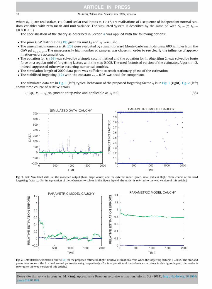
where h1; h2 are real scalars, r > 0 and scalar real inputs ut ; t 2 tH, are realisations of a sequence of independent normal ran-dom variables with zero mean and unit variance. The simulated system is described by the same pd with Hs ¼ ðh0s; rsÞ ¼ð½0:8;0:9�;1Þ.

The specialisation of the theory as described in Section 4 was applied with the following options:

� The prior GiW distribution (19) given by unit L0 and m0 was used.� The generalised moments at ;Bt (25) were evaluated by straightforward Monte Carlo methods using 600 samples from the

GiW pd pLt�1 ;mt�1þ1. The unnecessarily high number of samples was chosen in order to see clearly the influence of approx-imation-errors accumulation.� The equation for ~mt (26) was solved by a simple secant method and the equation for kt , Algorithm 2, was solved by brute

force on a regular grid of forgetting factors with the step 0.005. The used factorised version of the estimator, Algorithm 2,indeed suppressed otherwise occurring numerical troubles.� The simulation length of 2000 data pairs was sufficient to reach stationary phase of the estimation.� The stabilised forgetting (12) with the constant kc ¼ 0:95 was used for comparison.

The simulated data are in Fig. 1 (left), typical behaviour of the proposed forgetting factor kt is in Fig. 1 (right). Fig. 2 (left)shows time course of relative errors

Fig. 1.forgetti

Fig. 2.green lreferred

Pleasej.ins.2

ðE½hjLt ; mt � � hsÞ=hs ðmeant entry-wise and applicable as hs – 0Þ ð33Þ

0 500 1000 1500 2000−200

−100

0

100

200

300

400

500

600

700SIMULATED DATA CAUCHY

TIME

DAT

A

0 500 1000 1500 20000

0.1

0.2

0.3

0.4

0.5

0.6

0.7

0.8

0.9

1PARAMETRIC MODEL CAUCHY

TIME

FOR

GET

TIN

G F

ACTO

R

Left: Simulated data, i.e. the modelled output (blue, large values) and the external input (green, small values). Right: Time course of the usedng factor kt . (For interpretation of the references to colour in this figure legend, the reader is referred to the web version of this article.)

0 500 1000 1500 2000−0.2

0

0.2

0.4

0.6

0.8

1

1.2PARAMETRIC MODEL CAUCHY

TIME

REL

ATIV

E ES

TIM

ATIO

N E

RR

OR

S

0 500 1000 1500 20000

0.2

0.4

0.6

0.8

1

1.2

1.4PARAMETRIC MODEL CAUCHY

TIME

REL

ATIV

E ES

TIM

ATIO

N E

RR

OR

S

Left: Relative estimation errors (33) for the proposed estimator. Right: Relative estimation errors when the forgetting factor is k ¼ 0:95. The blue andines concern the first and second parameter entry, respectively. (For interpretation of the references to colour in this figure legend, the reader is

to the web version of this article.)





for the proposed estimator and Fig. 2 (right) shows the same quantities for the naive estimator combined with a fixedforgetting.

A range of experiments differing in noise distributions, their realisations and prior pd was performed. Their outcomeslooked quite similar. They confirmed that the presented results are typical and weakly dependent on the specific optionsmade. The high occurrence of the extreme forgetting factors in {0,1} is characteristic to the very heavy-tailed Cauchy para-metric model. The models with lighter tails are less demanding and infrequently require k ¼ 0: they rarely drop the updatingand projection pair.

6. Concluding remarks

Adaptive control [4] has been the author’s original research domain. There, the recursive treatment and adaptation tochanges dominate and a lot have been done in this area. Comparing to general cases, the processed data streams are theredefinitely simpler. The adaptive control, however, demonstrated that the common problems ranging from data preprocess-ing, detection of abrupt changing, adaptation to slow changes [25,26], dynamic clustering [16], etc. are systematically solv-able within a single axiomatised framework [18]. The current paper fills a significant gap of the referred theory by designinga recursive Bayesian estimator, which counteracts the accumulation of approximation errors caused by the recursivetreatment.

The proposed estimator is useful on its own. More importantly, it touches of the common problem of widely used recur-sive techniques like sequential Monte Carlo parameter estimation, variational Bayes, unscented-transformation based esti-mation, etc. The problem is especially urgent in the considered parameter estimation, where the errors are not damped by astable state evolution. Respecting these observations in the future research promises a non-trivial improvements of estab-lished estimators and filters. This hypothesis is supported by recent attempts of this type, e.g. [29].

A finer structuring of the circumscribing set is a promising direction of the future research. Ideas connected with direc-tional [25] and partial [10] forgetting are surely applicable.

Treatment of general data streams requires a systematic effort and corresponding expertise to get general algorithmicsolutions available now only in the simpler adaptive-control context. This paper intends to stimulate a wider research inter-est in this respect. Recent papers like [13], dealing with drifts in data streams, confirm the need for it. The same observationapplies to handling of crowd-wisdom-based classifiers [36], which obviously have to gradually switch from the batch toadaptive data-stream processing.

Acknowledgements

The research reflected in this paper has been supported by GACR 13-13502S. Dr. Kamil Dedecius helped significantly ininitial phase of the research that indicated we are on a proper track.

References

[1] M. Abramowitz, I.A. Stegun, Handbook of Mathematical Functions, Dover Publications, New York, 1972.[2] C. Aggarwal (Ed.), Data Streams: Models and Algorithms, Springer, 2007.[3] D.L. Alspach, H.W. Sorenson, Nonlinear Bayesian estimation using Gaussian sum approximation, IEEE Trans. Autom. Control 17 (4) (1972) 439–448.[4] K.J. Astrom, B. Wittenmark, Adaptive Control, Addison-Wesley, Massachusetts, 1989.[5] A. Benveniste, M. Métivier, P. Priouret, Adaptive Algorithms and Stochastic Approximations, Springer, Berlin, 1990.[6] L. Berec, M. Kárny, Identification of reality in Bayesian context, in: K. Warwick, M. Kárny (Eds.), Computer-Intensive Methods in Control and Signal

Processing, Birkhäuser, 1997, pp. 181–193.[7] J.O. Berger, Statistical Decision Theory and Bayesian Analysis, Springer, New York, 1985.[8] J.M. Bernardo, Expected information as expected utility, Ann. Stat. 7 (3) (1979) 686–690.[9] F. Daum, Nonlinear filters: beyond the Kalman filter, IEEE Aero. Electron. Syst. Mag. 20 (8) (2005) 57–69.

[10] K. Dedecius, I. Nagy, M. Kárny, Parameter tracking with partial forgetting method, Int. J. Adapt. Control Signal Process. 26 (1) (2012) 1–12.[11] A. Doucet, V.B. Tadic, Parameter estimation in general state-space models using particle methods, Ann. Inst. Stat. Math. 55 (2) (2003) 409–422.[12] M.M. Gaber, A. Zaslavsky, S. Krishnaswamy, Mining data streams: a review, SIGMOD Record 34 (2) (2005) 1–26.[13] J. Gama, I. Ziobailte, A. Bifet, ACM computing surveys, J. Math. Econ. 1 (1) (2013).[14] R. Horst, H. Tuy, Global Optimization, Springer, 1996. 727 pp..[15] S.J. Julier, J.K. Uhlmann, H.F. Durrant-Whyte, A new approach for the nonlinear transformation of means and covariances in linear filters, IEEE Trans.

Autom. Control 5 (3) (2000) 477–482.[16] M. Kárny, J. Böhm, T.V. Guy, L. Jirsa, I. Nagy, P. Nedoma, L. Tesar, Optimized Bayesian Dynamic Advising: Theory and Algorithms, Springer, 2006.[17] M. Kárny, T.V. Guy, On support of imperfect Bayesian participants, in: T.V. Guy, M. Kárny, D.H. Wolpert (Eds.), Decision Making with Imperfect

Decision Makers, vol. 28, Springer, Berlin, 2012. Intelligent Systems Reference Library.[18] M. Kárny, T. Kroupa, Axiomatisation of fully probabilistic design, Inform. Sci. 186 (1) (2012) 105–113.[19] L. Khan, Data stream mining: challenges and techniques, in: Proc. 22nd IEEE International Conference on Tools with Artificial Intelligence, 2010.[20] R. Kulhavy, A Bayes-closed approximation of recursive nonlinear estimation, Int. J. Adapt. Control Signal Process. 4 (1990) 271–285.[21] R. Kulhavy, Recursive Bayesian estimation under memory limitations, Kybernetika 26 (1990) 1–20.[22] R. Kulhavy, Recursive nonlinear estimation: a geometric approach, Automatica 26 (3) (1990) 545–555.[23] R. Kulhavy, Can approximate Bayesian estimation be consistent with the ideal solution?, in: Proc. of the 12th IFAC World Congress, vol. 4, Sydney,

Australia, 1993, pp. 225–228.[24] R. Kulhavy, Implementation of Bayesian parameter estimation in adaptive control and signal processing, Statistician 42 (1993) 471–482.[25] R. Kulhavy, M. Kárny, Tracking of slowly varying parameters by directional forgetting, in: Preprints of the 9th IFAC World Congress, vol. X, IFAC,

Budapest, 1984, pp. 178–183.[26] R. Kulhavy, M.B. Zarrop, On a general concept of forgetting, Int. J. Control 58 (4) (1993) 905–924.

Please cite this article in press as: M. Kárny, Approximate Bayesian recursive estimation, Inform. Sci. (2014), http://dx.doi.org/10.1016/j.ins.2014.01.048

http://refhub.elsevier.com/S0020-0255(14)00096-6/h0030











































[27] S. Kullback, R. Leibler, On information and sufficiency, Ann. Math. Stat. 22 (1951) 79–87.[28] H.J. Kushner, Stochastic Stability and Control, Academic Press, 1967.[29] F. Liu, D. Qian, C. Liu, An artificial physics optimized particle filter, Kong. yu Juece/Control Decis. 27 (8) (2012) 1145–1149.[30] M. Loeve, Probability Theory, van Nostrand, Princeton, New Jersey, Russian translation, Moscow, 1962.[31] P. Del Moral, A. Doucet, S.S. Singh, Forward smoothing using sequential Monte Carlo, Technical Report CUED/F-INFENG/TR 638, Cambridge University,

2010.[32] V. Peterka, Bayesian system identification, in: P. Eykhoff (Ed.), Trends and Progress in System Identification, Pergamon Press, Oxford, 1981. pp. 239–

304.[33] M.M. Rao, Measure Theory and Integration, John Wiley, NY, 1987.[34] I.N. Sanov, On probability of large deviations of random variables, Matemat. Sborn. 42 (1957) 11–44. also in Selected Translations Mathematical

Statistics and Probability I (1961) 213–244 (in Russian)..[35] J. Shore, R. Johnson, Axiomatic derivation of the principle of maximum entropy & the principle of minimum cross-entropy, IEEE Trans. Inform. Theory

26 (1) (1980) 26–37.[36] E. Simpson, S. Roberts, I. Psorakis, A. Smith, Dynamic Bayesian combination of multiple imperfect classifiers, in: T.V. Guy, M. Kárny, D.H. Wolpert

(Eds.), Decision Making and Imperfection, vol. 28, Springer, Berlin, 2013, pp. 1–38. Studies in Computation Intelligence.[37] V. Šmídl, A. Quinn, The Variational Bayes Method in Signal Processing, Springer, 2005.

Please cite this article in press as: M. Kárny, Approximate Bayesian recursive estimation, Inform. Sci. (2014), http://dx.doi.org/10.1016/j.ins.2014.01.048

























approximate bayesian recursive estimation

Documents