Nonlinear Vibrations of Metallic and Composite Structures

by

Tony 1. Anderson

Dissertation submitted to the Faculty of the

Virginia Polytechnic Institute and State University

in Partial fulfillment of the requirements for the degree of

Doctor of Philosophy

in

Engineering Mechanics

APPROVED:

Ali H. Nayfeh, Chai an

d~~~ DeanT.Mook Mahendra P. Singh

Rakesh K. Kapania Scott L. Hendricks

April 1993

Blacksburg, Virginia

Nonlinear Vibrations of Metallic and Composite Structures

by

Tony J. Anderson

Ali H. Nayfeh, Chairman

Engineering Mechanics

(ABSTRACT)

In this work, several studies into the dynamic response of structures are made.

In all the studies there is an interaction between the theoretical and experimental work

that lead to important results. In the first study, previous theoretical results for the

single-mode response of a parametrically excited cantilever beam are validated. Of

special interest is that the often ignored nonlinear curvature is stronger than the

nonlinear inertia for the first mode. Also, the addition of quadratic damping to the

model improves the agreement between the theoretical and experimental results. In

the second study, multi-mode responses of a slender cantilever beam are observed and

characterized. Here, frequency spectra, psuedo-phase planes, Poincare sections, and

dimension values are used to distinguish among periodic, quasi-periodic, and chaotic

motions. Also, physical interpretations of the modal interactions are made. In the

third study, a theoretical investigation into a previously unreported modal interaction

between high-frequency and low-frequency modes that is observed in some

experiments is conducted. This modal interaction involves the complete response of

the first mode and modulations associated with the third and fourth modes of the

beam. A model that captures this type of modal interaction is developed. In the

fourth study, the natural frequencies and mode shapes of several composite plates are

experimentally detennined and compared with a linear finite-element analysis. The

objective of the work is to provide accurate experimental natural frequencies of

several composite plates that can be used to validate future theoretical developments.

iii

Acknowledgments

I would like to thank my advisor, Professor Ali H. Nayfeh, for the opportunity to

work with him and for his guidance and support through my research. I would like to

thank Dr. Scott L. Hendricks for his friendship and help both at and away from school. I

would like to thank Professors Dean T. Mook and Mahendra P. Singh for their teaching

and advise. In addition, I would like to thank Rakesh K. Kapania for his helpful

comments about my work. I would like to thank Edmund G. Henneke and the ESM

Department for financial support. I would like to thank all the people at Virginia

Polytechnic Institute and State University who have taught me and provided an excellent

educational opportunity.

I would like to thank Balakumar Balachandran and Pemg-Jin F. Pai for their

freely given input to my work and for their friendship, and special thanks for Balakumar

Balachandran1s patience on reviewing my publications. I would like to express my

appreciation to Kyoyul Oh and the other students working in the Vibrations Laboratory

and Sally Shrader for their help and friendships that made my work more enjoyable.

I am most thankful to my wife and children. They provide both support for my

work and a life away from school that is required for the maintenance of my sanity.

This work was support by the Army Research Office under Grant No. DAAL03-

89-K-0180, the Center for Innovative Technology under Contract No. MAT-91-013, and

the Air Force Office of Scientific Research under Grant No. F49620-92-J-0197.

iv

Table of Contents

1. Introduction ................................................................................................................ 1

1.1 Literature Review ......................................................................................... 2

1.1.1 Beam Studies ................................................................................. 3

1.1.2 Damping ........................................................................................ 7

1.1.3 Nonlinear Dynamic Phenomena in Other Structures .................... 9

1.1.4 Composite Plate Studies ................................................................ 11

1.2 Summary and Overview of the Dissertation ............................................... 14

2. Test Setup and Tools .................................................................................................. 16

2.1 Nonlinear Equations of Motion .................................................................... 16

2.2 Test Setup and Measurements ...................................................................... 19

2.3 Tools for Characterizing Motions ................................................................ 23

2.3.1 Frequency Spectra .......................................................................... 24

2.3.2 Psuedo-Phase Plane ........................................................................ 26

2.3.3 Poincare Sections ........................................................................... 27

2.3.4 Pointwise Dimension ..................................................................... 28

3. Experimental Verification of the Importance of Nonlinear Curvature in the Response of a Cantilever Beam ................................................................................ 37

3.1 Multiple-Scales Analysis ............................................................................. 37

3.2 Experiments ................................................................................................. 44

3.3 Results .......................................................................................................... 45

3.4 Discussion and Conclusions ......................................................................... 48

4. Experimental Observations of the Transfer of Energy From High-Frequency Excitations to Low-Frequency Response Components ............................................ 55

4.1 Test Description ........................................................................................... 56

v

4.2 Planar Motion for fe =: 2f3 ............................................................................ 58

4.3 Out-of-Plane Motion for fe =: 2f3 .................................................................. 61

4.4 Band-Limited Random Base Excitation ...................................................... 62

4.5 Periodic Base Excitation: fe = 138 Hz and fe=144.0 Hz .............................. 63

4.6 Concluding Remarks .................................................................................... 65

5. Exchange of Energy Between Modes with Widely Spaced Frequencies: Theory and Experiment ............................................................................................. 79

5.1 Perturbation Analysis ................................................................................... 79

5.2 Theoretical Results ....................................................................................... 85

5.3 Comparison of Experimental and Theoretical Results ................................ 88

5.4 Concluding Remarks .................................................................................... 91

6. Natural Frequencies and Mode Shapes of Laminated Composite Plates: Experiments and FEM .............................................................................................. 101

6.1 Plate Descriptions ........................................................................................ 101

6.2 Test Setup and Analysis ............................................................................... 105

6.3 Results and Comparisons ............................................................................. 108

6.4 Summary and Discussion ............................................................................. 117

7. Summary and Recommendations .............................................................................. 147

7.1 Summary ...................................................................................................... 147

7.2 Recommendations ........................................................................................ 148

References..................................................................................................................... .. 150

Vita .................................................................................................................................. 159

vi

List of Figures

Fig. 2.1 A cantilever beam subjected to a base excitation ............................................. 31

Fig. 2.2 A schematic of the experimental setup for periodic excitation ........................ 32

Fig. 2.3 A schematic of the experimental setup for random excitation ......................... 33

Fig. 2.4 Frequency spectra of a periodic signal composed of two sine waves with the record length being an integer multiple of the periods ............................................. 34

Fig. 2.5 Plot for dimension calculation .......................................................................... 35

Fig 2.6 Plots of dimension versus embedding dimension for two scaling regions ........ 36

Fig. 3.1 Experimental and theoretical frequency-response curves for the first mode when C1 =0.000 and ab = 46.53 inlsecl\2 ............................................................... 49

Fig. 3.2 Experimental and theoretical force-response curves for the first mode when C1 =O.<XXl and fe=1.253 Hz ..................................................................................... 49

Fig. 3.3 Theoretical frequency-response curves for the first mode for ab = 46.53 inlsecl\2 and various values OfCl ................................................................ 50

Fig. 3.4 Theoretical force-response curves for the first mode for fe=1.253 Hz and various values of C 1 ........................................................................................................ 50

Fig. 3.5 Experimental and theoretical frequency-response curves for the first mode when C 1 =0.050 and ab = 46.53 inlsecI\2 .............................................................. 51

Fig. 3.6 Experimental and theoretical force-response curves for the first mode when C 1 =0.050 and fe= 1.253 Hz .................................................................................... 51

Fig. 3.7 Experimental and theoretical frequency-response curves for the second mode when C2=O'000 and ab = 61. 78 inlsecl\2 .............................................................. 52

Fig. 3.8 Experimental and theoretical force-response curves for the second mode when C2=O'OOO and 11.05 Hz ......................................................................................... 52

Fig. 3.9 Theoretical frequency-response curves for the second mode for ab = 61. 78 inlsecl\2 and various values of C2 ................................................................ 53

Fig. 3.10 Theoretical force-response curves for the second mode for fe=11.05 Hz and various values of C2 ................................................................................................. 53

Fig. 3.11 Experimental and theoretical frequency-response curves for the second mode when C2=O.100 and ab = 61. 78 inlsecl\2 .............................................................. 54

vii

Fig. 3.12 Experimental and theoretical force-response curves for the second mode when C2=O.I00 and fe=11.05 Hz .................................................................................... 54

Fig. 4.1 Cantilever beam response during a steady frequency sweep ............................ 67

Fig. 4.2 Power spectra and Poincare sections of the response during ........................... 68

Fig. 4.3 Strain-gage and base acceleration spectra for fe=32.00 Hz and ab=1.414 grms ................................................................................................................................. 71

Fig. 4.4 Strain-gage spectrum for fe=31.880 Hz and ab=1.414 grms ............................. 71

Fig. 4.5 Strain-gage spectrum for fe=31.879 Hz and ab=1.414 grms ............................. 72

Fig. 4.6 Time trace of a quasi-periodic motion for fe=31.879 Hz and ab=I.414 grms ................................................................................................................. 72

Fig.4.7 Strain-gage zoom span spectrum for fe=31.878 Hz and ab=1.414 grms .......... 73

Fig.4.8 Strain-gage spectrum for fe=31.877 Hz and ab=1.414 grms ............................. 74

Fig. 4.9 Poincare section for fe=31.880 Hz and ab=1.414 grms .................................... 74

Fig. 4.10 Time trace of a transient motion for fe=31.877 Hz and ab=1.414 grms ......... 75

Fig. 4.11 Strain-gage and base-acceleration spectrum for band-limited random excitation ....................................................................... 00 •• 00 •••••••••••••••••••••••••••••••••••••••••••• 76

Fig. 4.12 Strain-gage and base-acceleration spectrum for fe=138 Hz and ab=D.52 grms ................................................................................................................................. 77

Fig. 4.13 Strain-gage and base-acceleration spectrum for fe=l44 Hz and ab=O.52 grms ................................................................................................................................. 78

Fig. 5.1 Distribution force needed to produce the static deflection ~o(s) . ....•.............. 94

Fig. 5.2 Frequency-response curves: a) complete response of the first mode aI' b) amplitude of the third mode a3'1 and c) amplitude of the fourth mode a4' ••••••••••••••••••••••• 95

Fig. 5.3 Amplitudes of periodic solutions and magnitudes of nearby fixed points ........ 97

Fig. 5.4 Experimentally obtained stationary frequency-response curves ...................... 98

Fig. 5.5 An experimentally obtained frequency spectrum and a Poincare section for tIle three-mode motion ............................................................................................... 99

Fig. 5.6 Numerically obtained spectra and phase portraits obtained from the averaged equations .......................................................................................................... 100

Fig. 6.1 Free-hanging plate description and plate dimension definitions ...................... 119

viii

Fig. 6.2 Cantilever plate configuration .......................................................................... 120

Fig. 6.3 Fixed-fixed plate configuration ........................................................................ 120

Fig. 6.4 Details of the clamp used for the cantilever and fixed-fixed configurations .................................................................................................................. 121

Fig. 6.5 Schematic of the modal analysis test setup ....................................................... 122

Fig. 6.6 Contour plots of experimentally obtained mode shapes for the free-hanging ±15° plate configuration ............................................................................ 123

Fig. 6.7 Contour plots of experimentally obtained mode shapes for the free-hanging ±30° plate configuration ............................................................................ 124

Fig. 6.8 Contour plots of experimentally obtained mode shapes for the free-hanging cross-ply plate configuration ..................................................................... 125

Fig. 6.9 Contour plots of experimentally obtained mode shapes for the free-hanging quasi-isotropic plate configuration ............................................................ 126

Fig. 6.10 Contour plots of experimentally obtained mode shapes for the cantilevered ±15° plate configuration ............................................................................. 127

Fig. 6.11 Contour plots of experimentally obtained mode shapes for the cantilevered ±30° plate configuration ............................................................................. 128

Fig. 6.12 Contour plots of experimentally obtained mode shapes for the cantilevered cross-ply plate configuration ...................................................................... 129

Fig. 6.13 Contour plots of experimentally obtained mode shapes for the cantilevered quasi-isotropic plate configuration ............................................................. 130

Fig. 6.14 Contour plots of experimentally obtained mode shapes for the fixed-fIXed ±15° plate configuration ......................................................................................... 131

Fig. 6.15 Contour plots of experimentally obtained mode shapes for the fixed-fIXed ±30° plate configuration ......................................................................................... 132

Fig. 6.16 Contour plots of experimentally obtained mode shapes for the fixed-fIXed cross-ply plate configuration ................................................................................. 133

Fig. 6.17 Contour plots of experimentally obtained mode shapes for the fixed-fIXed quasi-isotropic plate configuration ........................................................................ 134

Fig. 6.18 Displacement plots of theoretically obtained mode shapes for the free-hanging ±15° plate configuration .................................................................................... 135

Fig. 6.19 Displacement plots of theoretically obtained mode shapes for the free-hanging ±30° plate configuration .................................................................................... 136

ix

Fig. 6.20 Displacement plots of theoretically obtained mode shapes for the free-hanging cross-ply plate configuration ............................................................................. 137

Fig. 6.21 Displacement plots of theoretically obtained mode shapes for the free-hanging quasi-isotropic plate configuration .................................................................... 138

Fig. 6.22 Displacement plots of theoretically obtained mode shapes for the cantilevered ±15° plate configuration ............................................................................. 139

Fig. 6.23 Displacement plots of theoretically obtained mode shapes for the cantilevered ±30° plate configuration ............................................................................. 140

Fig. 6.24 Displacement plots of theoretically obtained mode shapes for the cantilevered cross-ply plate configuration ...................................................................... 141

Fig. 6.25 Displacement plots of theoretically obtained mode shapes for the cantilevered quasi-isotropic plate configuration ............................................................. 142

Fig. 6.26 Displacement plots of theoretically obtained mode shapes for the fixed-fixed ±15° plate configuration ......................................................................................... 143

Fig. 6.27 Displacement plots of theoretically obtained mode shapes for the fixed-fixed ±30° plate configuration ......................................................................................... 144

Fig. 6.28 Displacement plots of theoretically obtained mode shapes for the fixed-flXed cross-ply plate configuration ................................................................................. 145

Fig. 6.29 Displacement plots of theoretically obtained mode shapes for the fixed-flXed quasi-isotropic plate configuration ........................................................................ 146

x

List of Tables

Table 2.1 Definitions of Variables ................................................................................. 17

Table 2.2 Physical Parameters of the Beam ................................................................... 21

Table 2.3 Beam Frequency Data .................................................................................... 21

Table 3.1 Valoes of Coefficients in Modulation Equations ........................................... 43

Table 6.1. Plate dimensions ........................................................................................... 103

Table 6.2 Plate material properties ................................................................................ 105

Table 6.3 CL T stiffness matrices for the four plates calculated using the average ply thickness of 0.0116 in ............................................................................................... 106

Table 6.4 Effective plate dimensions of the twelve configurations ............................... 107

Table 6.5 Modal analysis results and comparison with finite-element results for the free-hanging ±15° plate ............................................................................................. 112

Table 6.6 Modal analysis results and comparison with finite-element results for the free-hanging ±30° plate ............................................................................................. 113

Table 6.7 Modal analysis results and comparison with finite-element results for the free-hanging cross-ply plate ...................................................................................... 113

Table 6.8 Modal analysis results and comparison with finite-element results for the free-hanging quasi-isotropic plate ............................................................................. 114

Table 6.9 Modal analysis results and comparison with finite-element results for the ±15° cantilever plate .................................................................................................. 114

Table 6.10 Modal analysis results and comparison with finite-element results for the ±30° cantilever plate .................................................................................................. 115

Table 6.11 Modal analysis results and comparison with finite-element results for the cross-ply cantilever plate ........................................................................................... 115

Table 6.12 Modal analysis results and comparison with finite-element results for the quasi-isotropic cantilever plate ................................................................................. 116

Table 6.13 Modal analysis results and comparison with finite-element results for the ±15° fixed-fixed plate ................................................................................................ 116

Table 6.14 Modal analysis results and comparison with finite-element results for the ±30° fixed-fixed plate ................................................................................................ 117

xi

Table 6.15 Modal analysis results and comparison with finite-element results for the cross-ply fixed-fixed plate ......................................................................................... 117

Table 6.16 Modal analysis results and comparison with finite-element results for the quasi-isotropic fixed-fixed plate ............................................................................... 118

XlI

1. Introduction

Performance requirements for structures are becoming more difficult to meet.

Often the requirements on structures are conflicting. For example, due to the expense of

carrying components into orbit, the structure for the Space Station Freedom must be light

weight. In addition, low-gravity experiments require stable platforms. The Hubble Space

Telescope required light-weight components and extremely tight pointing accuracy.

Mter the Hubble Space Telescope was in orbit and operating, scientists found that low­

frequency structural vibrations initiated by the release of thermal stresses were large

enough that the pointing accuracy did not meet the requirements of the observation

missions and valuable time was lost due to the vibrations. Light weight and high strength

are requirements for structures, such as the blades of hubless helicopter rotors. This

certainly is not an all inclusive list of high-performance structures, but it is enough to

show that the requirements on these structures are contradictory. For example, the easiest

way for engineers to make a stable platform for the space station is to make it big and

stiff and not worry about the structure's dynamics, but this violates the other requirement

of light-weight components. This trend of ever more difficult requirements on structures

is sure to continue.

Engineers must consider the dynamics in the modeling of a structure in order to

meet high-performance requirements. Linear models are often used to approximate the

response of structures. Linear models have many desirable characteristics. For many

linear systems, exact solutions are known and a single solution exists for a given set of

parameters. Also, superposition holds, modes do not exchange energy, and the frequency

content of the steady-state response is the same as that of the excitation. Light-weight

structures tend to be flexible. As the flexibility of structures increases, linear

approximations often no longer adequately predict the behavior and engineers must resort

to nonlinear models. This leads to a fundamental problem; the aforementioned

characteristics of linear systems do not hold for nonlinear systems.

When engineers deal with systems that require nonlinear models, they generally

resort to approximate techniques. The books by Nayfeh and Mook (1979), Bolotin

(1964), Evan-Ivanowski (1976), and Tondl (1965) show some of the tremendous amount

of work and success in this area. The responses of nonlinear systems exhibit complicated

phenomena, such as multiple solutions, frequency entrainment, superharmonic

resonances, subharmonic resonances, combination resonances, modal interactions,

saturation, quenching, Hopf bifurcations, limit cycles, symmetry-breaking and period­

multiplying bifurcations, and chaos. Even with this long list of different phenomena,

there is apparently no way of knowing if all types of nonlinear phenomena that can occur

have been found. Due to the approximate nature of the analytical techniques and the

many possible types of responses, it is difficult for an engineer to know with a high level

of confidence that the analytical results will capture the motion that will occur in practice.

This leads to the need for experiments to validate predicted results. In the process,

experiments can reveal previously unknown nonlinear responses.

1.1 Literature Review

Often, knowledge about nonlinear systems develops by the observation of a

phenomenon that is not understood, which leads to an analysis that explains the

observation, which in tum predicts additional phenomena not previously observed, which

is verified by experimental observations. A description of a classic example of this

process follows. Froude (1863) reported that a ship whose frequency in heave is twice its

frequency in roll has undesirable seakeeping characteristics. N ayfeh, Mook, and

Marshall (1973) considered the response of a ship whose frequency in pitch is

Chapter 1 2

approximately twice its frequency in roll to primary-resonant excitations. They found

nonlinear periodic and modulated responses when the first (roll) mode was excited by a

primary-resonant excitation. This type of response could be interpreted as undesirable

seakeeping characteristics. In their study, they also discovered the saturation

phenomenon. Haddow, Barr, and Mook (1984) conducted a theoretical and experimental

investigation of the response of a two-degree-of-freedom beam structure to a harmonic

excitation. They were the first to experimentally verify the saturation phenomenon.

Examples of theory and experiments complimenting each other are common

throughout the literature on nonlinear systems. A review of pertinent works on the

nonlinear vibration of structures follows.

1.1.1 Beam Studies

The exact analysis of structures is a nonlinear three-dimensional elasticity

problem. This is an extremely difficult problem for engineers. Typically, the analyst

makes some approximations to simplify the problem. For beam-like structures, beam

theories are very useful tools that reduce the three-dimensional elasticity problem to a

one-dimensional problem. The simplest beam theory is the well known Euler-Bernoulli

beam theory and can be found in any strength of materials text. It is applicable to the in­

plane deflections of long-slender isotropic beams. For this case, the shear deflection and

nonlinearities are ignored. For beams with high aspect ratios hIL, where h and L are the

length and thickness of the beam, respectively, or short wavelengths, the shear deflection

is not negligible. In these cases a first-order shear theory, known as Timoshenko's beam

theory (Thomson, 1981; Timoshenko, 1921, 1922), is often used. In this theory, the shear

stress is assumed to be the same at every point over a given cross section. A shear

correction coefficient, which depends on the shape of the cross section, is introduced to

account for the fact that the shear stress and shear strain are not uniformly distributed

Chapter 1 3

over the cross section. Heyliger and Reddy (1988) presented a higher-order shear

defonnation theory, in which some quadratic tenns are included and no shear correction

coefficient is needed.

Often nonlinearities due to finite deflections are important in the study of the

response of beam structures. Eringen (1951) included nonlinear inertia tenns in his

investigation of the planar response of simply-supported beams. He investigated the

single-mode response of a simply-supported beam with immovable hinged ends.

Evensen and Evan-Iwanowski (1966) included the effect of longitudinal inertia on the

parametric response of an elastic column. They assumed an inextensional beam and a

single-mode response. Their study combined analytical and experimental investigations

and found good agreement between the two. Sato et al. (1978) included both geometric

and inertia nonlinearities in their study of the parametric response of a horizontal beam

carrying a concentrated mass under gravity. They assumed a planar single-mode

response. Their results show that, in addition to parametric resonances, external

resonances occur due to initial static deflections.

The previously mentioned studies of the nonlinear response of beams investigated

planar responses. In the development of beam theories in three-dimensional space,

studies that combine theoretical and experimental results have proven to be important.

Haight and King (1971) analytically and experimentally investigated the stability of the

planar response of a parametrically excited cantilever beam. In the analysis, the three­

dimensional motion of a beam with approximately equal moments of inertia was

considered. For this case, the twisting of the beam can be neglected. Haight and King

found regions of forcing and frequency values that resulted in the planar motion losing

stability, resulting in an out-of-plane motion. Hodges and Dowell (1974) used Hamilton's

principle and Newton's second law to develop a comprehensive set of equations with

quadratic nonlinearities that describe the dynamics of beams in three-dimensional space.

Chapter 1 4

Dowell, Traybar, and Hodges (1977) devised a simple experiment to investigate the static

deflections and natural frequency shifts to evaluate the theory of Hodges and Dowell

(1974). The results show that there are systematic differences between the theory and

experiment when tip deflections become large. Later Hodges et al. (1988) pointed out

that the nonlinear equations of motion governing flexural deformations cannot be

consistent unless all nonlinear terms through third order are included. Crespo da Silva

and Glynn (1978a) formulated a set of consistent governing differential equations of

motion describing the nonplanar, nonlinear dynamics of an inextensional beam. In order

to include the twisting of the beam, they used three Euler angles to relate the deformed

and undeformed states. They also included nonlinearities due to both inertia and

curvature. Crespo da Silva and Glynn (1978b) showed that when the lower frequency

modes are considered the often ignored nonlinearities due to curvature are important. Pai

and Nayfeh (1992) presented a very general beam theory valid for metallic and

composite beams. The twisting curvature of the beam was used to define a twist angle,

resulting in equations of motion that are independent of the rotation sequence of the Euler

angles. They included both inertial and geometric nonlinearities as well as a third-order

shear-deformation model.

Several studies experimentally investigated the response of slender cantilever

beams similar to the one we study in this dissertation. Dugundji and Mukhopadhyay

(1973) experimentally and theoretically investigated the response of a thin cantilever

beam excited by a base motion transverse to the axis of the beam and along the direction

of the beam's larger cross-section dimension. They observed three resonances: a primary

resonance of the first torsional mode, a combination resonance involving the first and

second bending modes, and a combination resonance involving the first bending and first

torsional modes. For the cOITlbination resonance involving the first bending and first

torsional modes, the frequency relationship between the excitation frequency and the

Chapter 1 5

lowest-frequency component in the response was 18:1. Dugundji and Mukhopadhyay's

study demonstrates that high-frequency excitations can excite low-frequency modes

through external combination resonances. This type of resonance can be explained with

current analytical models. Haddow and Hasan (1988) experimentally investigated the

response of a parametrically excited flexible cantilever beam to an excitation whose

frequency was near twice the fourth natural frequency (2f4) and found various periodic

and chaotic responses. They also reported that an "extremely low subharmonic response"

occurred under certain conditions. Burton and Kolowith (1988) analytically and experi­

mentally studied the response of a parametrically excited flexible cantilever beam to an

excitation having a frequency near 2f4• They obtained experimental results similar to

those reported by Haddow and Hasan (1988). In the studies of Haddow and Hasan

(1988) and Burton and Kolowith (1988), prior to a chaotic response, a single-mode

periodic response was observed. Cusumano and Moon (1989) and Cusumano (1990)

presented results for an externally excited cantilever beam. They observed a "cascading

of energy" to low-frequency components in the response after the planar motion lost

stability, resulting in a nonplanar chaotic motion. The transition to a non planar chaotic

motion was the focus of the works of Haddow and Hasan (1988), Burton and Kolowith

(1988), and Cusumano and Moon (1989).

Several experimental studies have focused on chaotic vibrations of elastic beams.

Moon and Holmes (1979), Moon (1980), and Moon and Holmes (1985) investigated the

planar motion of buckled beams. In these test setups, the beam had two static equilibrium

positions. This lead to a two-well potential problem. The beam would vibrate about a

static equilibrium but then chaotically jump from one equilibrium to another. Moon and

Shaw (1983) experimentally and theoretically investigated chaotic vibrations in a planar

beam with impact boundary conditions.

Chapter 1 6

Cusumano (1990) extensively studied a slender cantilever beam subjected to an

external base excitation. His work focused mainly on chaotic out-of-plane motions. He

characterized these motions with time histories, frequency spectra, and dimension

calculations. In the excitation frequency-amplitude plane, he observed seven regions

where chaotic motions occurred. In all of the cases, the loss of planar stability was

preceded by the first in-plane bending mode being excited. He did not investigate how

the first mode was excited. For the modeling of the system, he set the curvature

associated with the largest area moment of inertia equal to zero. This defined a nonlinear

mode that consisted of out-of-plane bending and twisting. His experiment using a near

circular rod to verify this assumption is erroneous because, for this case, the assumption

of zero curvature is not valid. One area moment of inertia must be much larger than the

other to make this assumption. Cusumano also found that when the damping of the

system was reduced, the qualitative nature of the motion of the beam did not change. He

tested this by conducting experiments in a bag filled with helium. This suggests that the

damping model will change the analytical results quantitatively but not qualitatively.

1.1.2 Damping

Damping is a crucial element in the dynamics of structures. Without damping,

transient motions would not die out. Damping can also affect the stability boundaries.

Despite its importance, a well defined method for determining the type of dominant

damping mechanisms that are involved in a structure does not seem to exist. This is due,

in part, to the large number of possible mechanisms involved. Linear viscous damping is

often chosen because of modeling convenience. We present a brief review of studies on

damping to give some insight into the topic and present a background for the selection of

the damping models.

Chapter 1 7

Bert (1973) reviewed material damping models. He compared the energy loss per

cycle of the models and discussed their shortcomings. Also discussed are various

measurement techniques. Crandall (1970) discussed damping mechanisms and presented

results that show that damping depends on the amplitude and frequency of cyclic

motions. He described some models and noted their limitations. He also presented

examples where damping affects the stability of the dynamical system. Nelson and Greif

(1970) reviewed which of these models was incorporated into general purpose shock and

vibration computer programs.

Because the mechanisms involved in damping are not very well known,

experiments are typically conducted to determine the damping coefficients. Generally the

form of the damping is assumed and the coefficients are determined. Baker, Woolam,

and Young (1967) investigated damping of thin cantilever beams. They introduced

internal damping and external air damping into the governing equations. They obtained

solutions by energy methods and computer simulations. Predicted decrements of free­

vibration decay were compared with experiments on cantilevers run in atmospheres with

standard and reduced pressures. Banks and Inman (1991) investigated damping

mechanisms in composite beams. They found that a spatial hysteresis model combined

with a linear viscous air damping model results in the best quantitative agreement with

experimental time histories. Adams and Bacon (1973) investigated the flexural damping

capacity and dynamic Young's modulus of metals and reinforced plastics. They tested

their specimens in vacuum in order to obtain material damping properties. Rades (1983)

presented two methods to determine coefficients for linear viscous and drag-type

quadratic damping. These methods were based on variations to polar plots due to the

quadratic damping. Rice and Fitzpatrick (1991) presented a method to determine

nonlinear elements in a system by reformulating the nonlinear problem as a multiple

input/output linear system. They applied the method to a single-degree-of-freedom

Chapter 1 8

system with a drag-type quadratic damping. All these studies point out the large effect air

damping can have on a system. The models assumed for air damping are linear viscous

or linear viscous and quadratic damping. These are the models used in this work.

1.1.3 Nonlinear Dynamic Phenomena in Other Structures

In this section, we give a brief review of studies that investigated nonlinear

phenomena in structures other than cantilever beams. The review emphasizes but is not

restricted to studies with experimental and theoretical work.

Evan-Iwanowski (1976) presented quite general theoretical results for various

nonlinear systems. These results were used to guide theoretical and experimental results

presented later in the text. He presented theoretical and experimental results for the cases

of principal parametric resonance (fe = 2fj) of a simply-supported plate, principal

parametric and summation combination resonances (fe=fi+fj) of a circular cylinder,

summation combination resonances(fe=fi+fj+fk} of a three-degree-of-freedom lumped

mass system with cubic nonlinearities, principal parametric resonance of a column, and

electric motor and cantilever beam interaction, where fe is the excitation frequency and

the fm are the natural frequencies of the system.

Haddow, Barr, and Mook (1984) theoretically and experimentally investigated the

response of an ttL" shaped structure to a harmonic excitation. The structure had two

lumped masses which had the effect of reducing the continuous system to a two-degree­

of-freedom system having the frequencies ft and f2. The dominant nonlinearities in the

system were quadratic. They observed the influences of a two-to-one internal resonance

(i.e., f2=2ft). They were also the [rrst to experimentally verify the saturation phenomenon

when fe=f2' Nayfeh and Zavodney (1988) experimentally observed amplitude- and

phase-modulated motions in a similar structure when fe=flo Nayfeh, Balachandran,

Colbert, and Nayfeh (1989) studied a similar "L" shaped structure. Balachandran (1990)

Chapter 1 9

and Balachandran and Nayfeh (1990) treated the beam sections of the structure as

continuum, and used a time-averaged Lagragian to obtain the governing equations of

motion. They found that, in the presence of autoparametric resonances, extremely small

excitation levels may to produce chaotic motions, whereas large excitation levels are

required to produce chaotic motions in single-degree-of-freedom systems.

Nayfeh (1983) investigated the response of a bowed structure (systems with

quadratic and cubic nonlinearities) to a combination resonance. He showed that the

combination resonance of the difference type can never be excited. He also found that,

for certain ranges of the forcing level and phase, the combination resonance can be

quenched or enhanced. Nayfeh (1984) studied the response of bowed structures to a two­

frequency excitation with no internal resonances. He found up to seven equilibrium

solutions. However, only one of these solutions is stable. He also found that when the

amplitude of the excitation is higher than that necessary for both modes to be nonzero,

there were no periodic steady-state responses.

Nayfeh, Nayfeh, and Mook (1990) investigated a T-shaped beam-mass structure

subjected to a harmonic excitation of the third mode. The first three natural frequencies

of the structure are such that the third natural frequency is approximately the sum of the

first and second natural frequencies. The experiments and associated analysis show the

existence of modal saturation, quasiperiodic, and phase-locked responses.

Miles (1965), Anand (1966), Narasimha (1968), and Nayfeh and Mook (1979)

analyzed motions of strings subjected to harmonic in-plane excitations and found that

nonplanar responses are possible for some excitation frequencies. Johnson and Bajaj

(1989) investigated the same problem and showed that periodically and chaotically

modulated responses are possible. Nayfeh, Nayfeh, and Mook (1992) experimentally

investigated the motion of a stretched string subjected to external and parametric

excitations. The combination of parametric and external excitations leads to whirling

Chapter 1 10

motions where modes at the excitation frequency as well as modes at one-half the

excitation frequency can be excited. They showed that under certain conditions the

whirling motions lose stability, giving rise to complicated modulated motions.

1.1.4 Composite Plate Studies

To meet the ever more stringent requirements placed on structures, engineers

often use advanced composite materials because of their high specific moduli and high

specific weights. Much of the research on composite structures has been on plates.

Leissa (1981) surveyed the literature on the vibration and buckling of composite

plates. Bert (1985) reviewed the dynamic response of laminated composites. Reddy

(1983, 1985) reviewed the literature concerning the application of the finite-element

method for the vibration of plates. Kapania and Raciti (1989a,b) presented a summary of

recent advances in the analysis of laminated beams and plates. They reviewed the free­

vibration analysis of symmetrically laminated plates for various geometric shapes and

edge conditions.

In the study of the vibrations of laminated composite plates, the shear deflection is

important because of the large ratio between the tensile and shear moduli. Kapania and

Raciti (1989a) reviewed developments in the analysis of laminated beams and plates with

an emphasis on shear effects and buckling. They presented a discussion of various shear­

deformation theories for plates and beams and a review of the recently developed finite­

element method for the analysis of thin and thick laminated beams and plates. Librescu

and Reddy (1989) compared several shear-deformation theories and showed their

connection with first-order shear-deformation theory. Reddy (1984) and Bhimaraddi and

Stevens (1984) presented a higher-order shear-deformation theory that contains the same

dependent unknowns as the first-order shear-deformation theory, but accounts for a

parabolic distribution of the transverse shear strains through the thickness of the plate. It

Chapter 1 11

also predicts zero shear on the surface of the plate and does not require a shear correction

factor.

Bert and Mayberry (1969) experimentally and theoretically investigated the

natural frequencies and mode shapes of laminated anisotropic plates with clamped edges.

They presented the material properties used in the analysis but did not indicate how these

were obtained. They used the maximum response amplitude as a criterion to determine

the natural frequencies. In the theoretical investigation they neglected shear deflections

and used a Rayleigh-Ritz approximation. The error between the experimental and

theoretical results was approximately 10%. Clary (1972) investigated the natural

frequencies and mode shapes of unidirectional composite material panels. He

investigated the change in frequencies and mode shapes as the angle between the fibers

and boundaries is changed. He presented the material properties used in the analysis but

did not indicate how these were obtained. He used the maximum response amplitude to

determine the natural frequencies. Also, relatively large masses were attached to the

plate to monitor the response and to excite the plate. The percentage error between

experiment and theory is between 2% and 3% for the beam-type modes and between 2%

and 10% for the plate modes. Crawley (1979) experimentally and theoretically

investigated the natural frequencies and mode shapes of composite cantilever plates and

shells. He used the 90° phase difference between the periodic excitation and the response

as a criterion to determine the natural frequencies. This is a somewhat better method than

the maximum response amplitude method previously mentioned. He obtained material

properties from static tests of the specimens. The difference between experimental and

theoretical natural frequencies is approximately 12%. He suggested the difference could

be due to the dynamic moduli being different from the static moduli. Ashton and

Anderson (1969) experimentally and theoretically investigated the natural frequencies

and mode shapes of laminated boron-epoxy plates with clamped edges. They sprinkled

Chapter 1 12

aluminum granules on the plates. They took the excitation frequency at which the

granules had definite model patterns to be the natural frequency. The error between the

theoretical and experimental values for the natural frequencies ranges between 1-30 %.

There have been very few experimental investigations of the nonlinear response

of composite plates. Mayberry and Bert (1968) experimentally and theoretically

investigated the nonlinear vibrations of composite plates. They investigated a glass­

epoxy plate clamped on all edges. They observed that the plates frequencies increased as

the excitation level was increased. The predicted linear natural frequencies did not match

the measured linear natural frequencies. They normalized the results so that they match

in the linear case, then they found that the trend of increase in frequency with excitation

levels between theory and experiment matched for one case. The other cases did no

match.

Yamaki and Chiba (1983a, 1983b) experimentally and theoretically investigated

the nonlinear response of a thin isotropic rectangular plate clamped on all edges. They

observed many types of responses, such as internal and combination resonances. The

theory and experiments matched for some cases but not for most. The main limitation of

the analysis was their assumption that three symmetric modes participated in the

response. For most of the cases observed in the experiments, other modes participated in

the response.

The nonlinear analysis of laminated composite plates has been a subject of

significant current interest. Whitney (1968) and Whitney and Leissa (1969) were the first

to formulate the equations of motion for the large-deflection behavior of laminated

anisotropic plates by accounting for the von Karman geometrical nonlinearity. Chia

(1980) presents in his text a comprehensive literature review, which covers the work in

the field until 1979. Most nonlinear plate theories (Schmidt 1977; Reissner 1948, 1953;

Reddy 1984; and Bhimaraddi 1987) account for von Karman type nonlinearities with

Chapter 1 13

classical plate theory as well as first-order and higher-order shear theories. Pai and

Nayfeh (1991) presented a theory that accounts for nonlinear curvatures, mid-plane

strains, and third-order shear deformations. Singh, Rao, and Iyengar (1991) showed that

it is important to include nonlinearities in the analysis of composite plates even for small

loads because they observed nonlinear effects even in the small-deflection range

1.2 Summary and Overview of the Dissertation

In this work, several studies were conducted that combined experimental and

theoretical investigations. I believe the most significant results are presented in Chapters

4 and 5. In these Chapters, we present results pertaining to a newly found modal

interaction. This modal interaction could have implications for any structure that has

excitations with frequencies that are high relative to the lowest natural frequencies of the

structure. Following is an overview of the Dissertation.

In Chapter 2, we present the starting points for the investigation of the motion of

the metallic cantilever beam. For the theoretical investigation of the beam, we start with

the nonlinear equation and boundary conditions governing the planar motion of an

isotropic cantilever beam in a nondimensionalized and scaled form. For the experimental

investigation of the beam, we start with the test set-up and instrumentation. We also

present the tools used to characterize both the theoretical and experimental responses.

In Chapter 3, we present a theoretical and experimental investigation of single­

mode motions of the beam in the presence of a principal parametric resonance; that is, the

excitation frequency fe is near twice a natural frequency fi of the beam and the base

motion is along the undeformed axis of the beam. The nonlinearities in the system are

due to both nonlinear inertia (a softening-type nonlinearity) and the often ignored

nonlinear curvature (a hardening-type nonlinearity). Hence, the nonlinearity is of the

hardening or softening type depending on whether the curvature or inertia nonlinearity

Chapter 1 14

dominates the response. We experimentally verified that the nonlinearity for the first

mode is of the hardening type due to the dominance of the nonlinear curvature. Also, we

observed that the second mode is of the softening type, which is due to the dominance of

the nonlinear inertia.

In Chapter 4, we present the results of experimental investigations into the

transfer of energy from high-frequency excitations to low-frequency components in the

response of the flexible cantilever beam. Four cases were considered, three with periodic

base motions along the axis of the beam, and one with a band-limited random base

motion transverse to the axis of the beam. A transfer of energy from high-frequency

modes of the system to low-frequency modes of the system was observed in all four

cases.

In Chapter 5, we present a theoretical investigation of the resonances reported in

Chapter 4. We used the method of averaging to obtain equations that describe the

evolution of the slowly varying terms in the system. A nonclassical transformation is

used in the variation of parameters prior to the averaging process. This transformation

was required to capture the slow-time scale evolution of the low-frequency first mode

compared to the high-frequency third and fourth modes. The theoretical and

experimental results are in good agreement.

In Chapter 6, we present the results of an experimental and theoretical

investigation into the vibrations of advanced composite plates. We obtain the natural

frequencies and mode shapes of composite plates with several layup sequences and

boundary conditions. These results are compared to results obtained from linear finite­

element models. For the cases where the boundary conditions are well known, the

present experimental and finite-element results are in better agreement than what has

been previously reported.

Chapter 1 15

2. Test Setup and Tools

In this chapter, we introduce items that are common to Chapters 3-5. These items

include the nonlinear equations of motion for a flexible metallic cantilever beam, the test

setup used to investigate the nonlinear vibrations of the beam, and the tools used to

characterize the motions of the beam. Work on composite plates is presented in

Chapter 6, it is essentially self contained and includes a description of the test setup and

system.

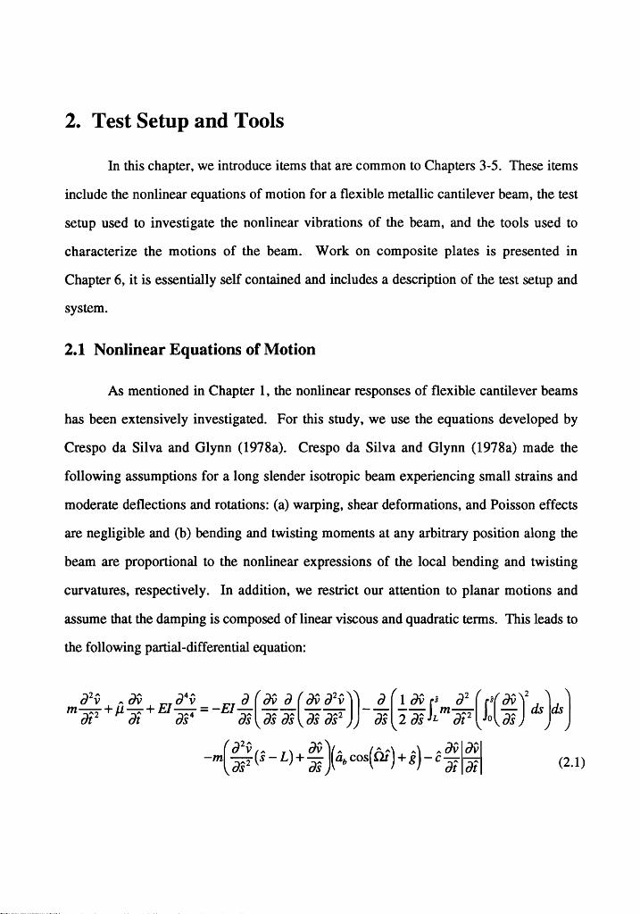
2.1 Nonlinear Equations of Motion

As mentioned in Chapter 1, the nonlinear responses of flexible cantilever beams

has been extensively investigated. For this study, we use the equations developed by

Crespo da Silva and Glynn (1978a). Crespo da Silva and Glynn (1978a) made the

following assumptions for a long slender isotropic beam experiencing small strains and

moderate deflections and rotations: (a) warping, shear deformations, and Poisson effects

are negligible and (b) bending and twisting moments at any arbitrary position along the

beam are proportional to the nonlinear expressions of the local bending and twisting

curvatures, respectively. In addition, we restrict our attention to planar motions and

assume that the damping is composed of linear viscous and quadratic terms. This leads to

the following partial-differential equation:

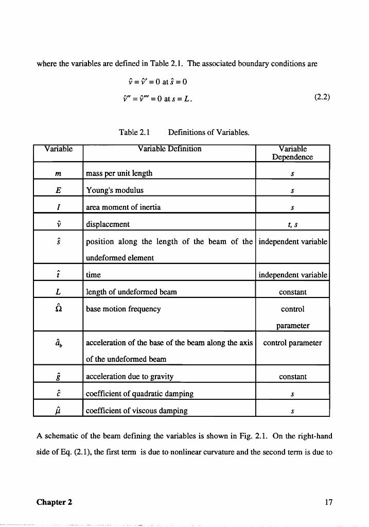
where the variables are defined in Table 2.1. The associated boundary conditions are

v = Vi = 0 at S = 0

V" = v'" = 0 at s = L. (2.2)

Table 2.1 Definitions of Variables.

Variable Variable Definition Variable Dependence

m mass per unit length s

E Young's modulus s

I area moment of inertia s

" displacement t, S v

" position along the length of the beam of the independent variable S

undeformed element

" time independent variable t

L length of undeformed beam constant

Q base motion frequency control

parameter

ab acceleration of the base of the beam along the axis control parameter

of the un deformed beam

g acceleration due to gravity constant

C coefficient of quadratic damping S

[L coefficient of viscous damping S

A schematic of the beam defining the variables is shown in Fig. 2.1. On the right-hand

side of Eq. (2.1), the first term is due to nonlinear curvature and the second term is due to

Chapter 2 17

nonlinear inertia. The third term represents the parametric excitation due to the base

motion and the effect of gravity. The last term is due to quadratic damping.

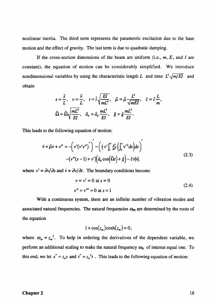
If the cross-section dimensions of the beam are uniform (Le., m, E, and I are

constant), the equation of motion can be considerably simplified. We introduce

non dimensional variables by using the characteristic length L and time L2 ~ m/ EI and

obtain

s v s=- v=-

L' L' ,,(EI - " L2

t = t~-;;;[J' J1 = J1 ~mEI'

This leads to the following equation of motion:

,

v+jiv+vw = {v'(v'v")') -(tvJ ~(J: V'2dY)dY)

-( v" (s - 1) + v')( iib cos( o't ) + g) - cVjVj.

_ "L C=C-,

m

where v' = avlas and v = avlat. The boundary conditions become

v = v' = 0 at s = 0

v" = VIII = 0 at s = 1

(2.3)

(2.4)

With a continuous system, there are an infinite number of vibration modes and

associated natural frequencies. The natural frequencies lDm are determined by the roots of

the equation

1 + cos{zm}cosh{zm} = 0,

where wm = Zm 2

• To help in ordering the derivatives of the dependent variable, we

perform an additional scaling to make the natural frequency ron of interest equal one. To

this end, we let s· = Z"s and t· = ZII 2t • This leads to the following equation of motion:

Chapter 2 18

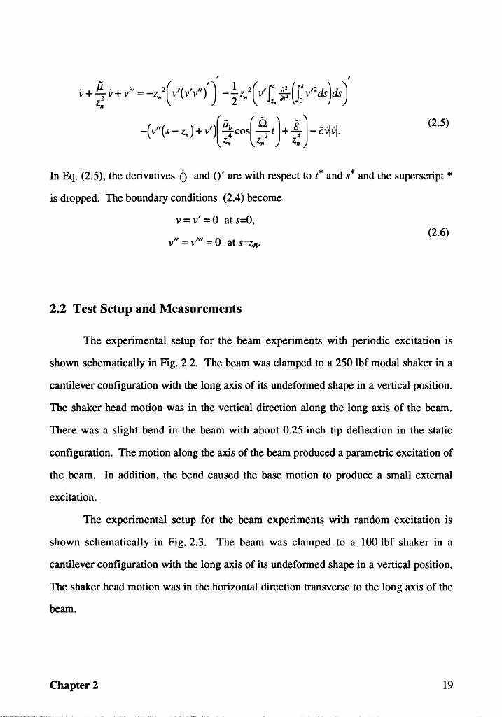
(2.5)

In Eq. (2.5), the derivatives () and 0" are with respect to t* and s* and the superscript * is dropped. The boundary conditions (2.4) become

v = v' = 0 at s=O,

v" = v'" = 0 at S=Zn. (2.6)

2.2 Test Setup and Measurements

The experimental setup for the beam experiments with periodic excitation is

shown schematically in Fig. 2.2. The beam was clamped to a 250 lbf modal shaker in a

cantilever configuration with the long axis of its undeformed shape in a vertical position.

The shaker head motion was in the vertical direction along the long axis of the beam.

There was a slight bend in the beam with about 0.25 inch tip deflection in the static

configuration. The motion along the axis of the beam produced a parametric excitation of

the beam. In addition, the bend caused the base motion to produce a small external

excitation.

The experimental setup for the beam experiments with random excitation is

shown schematically in Fig. 2.3. The beam was clamped to a 100 lbf shaker in a

cantilever configuration with the long axis of its undeformed shape in a vertical position.

The shaker head motion was in the horizontal direction transverse to the long axis of the

beam.

Chapter 2 19

The test specimen was a carbon steel beam with dimensions 33.56" x 0.75" x

0.032 ". In Table 2.2, we summarize the physical properties of the beam. The resulting

length to thickness ratio was 1049 and the width to thickness ratio was 23.44. Strain

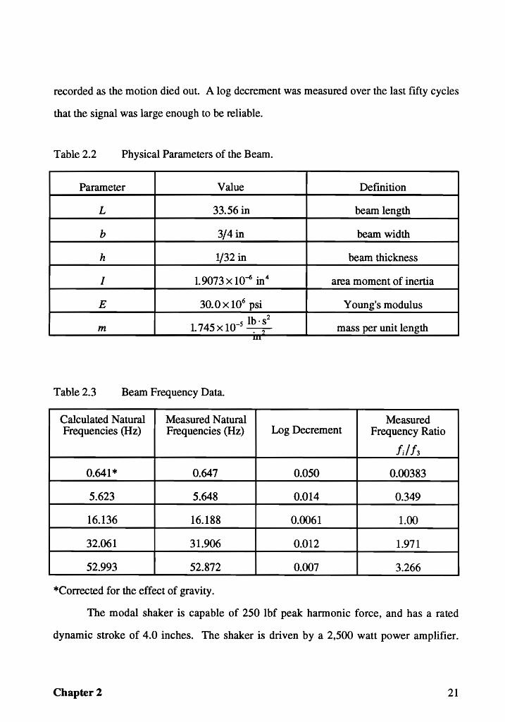
gages were used to obtain a measure of the beam response. In Table 2.3, we present the

first five measured and calculated natural frequencies along with the measured log

decrements. Because the third mode was a main component of several of the responses,

the frequency ratios relative to the third modes natural frequency are also given in

Table 2.3.

Because the base motion was along the long axis of the beam and hence produced

a parametric excitation, common frequency-domain methods of experimental modal

analysis cannot be used to measure natural frequencies and damping values (Ewins,

1984). To measure the frequencies, we excited the beam at approximately twice the

natural frequency of interest, thereby excited the associated mode in a principal

parametric resonance. We then stopped the excitation and monitored the locations of

peaks in the response spectrum that was continually updated. As the amplitudes of the

peaks shrank into the noise floor, we noted the frequencies. We used an additional

method to measure the natural frequency of the first mode (Zavodney 1987). We plotted

on the oscilloscope the output of the signal generator versus a strain-gage signal after the

excitation was turned off to produce a Lissajous pattern. The frequency from the signal

generator was adjusted until the figure eight was stationary. We interpreted the frequency

setting of the signal generator to be twice the first natural frequency. The results of this

method agree with those obtained by using the frequency-spectrum method. A similar

procedure was used to measure the damping. The beam was excited at twice the natural

frequency of the mode of interest. The excitation was turned off and a time history was

Chapter 2 20

recorded as the motion died out. A log decrement was measured over the last fifty cycles

that the signal was large enough to be reliable.

Table 2.2 Physical Parameters of the Beam.

Parameter Value Definition

L 33.56 in beam length

b 3/4 in beam width

h 1/32 in beam thickness

I 1.9073 x 10-6 in4 area moment of inertia

E 30.0 x 106 psi Young's modulus

m 1. 745 x 10-5 l~' ~2 mass per unit length .... n

Table 2.3 Beam Frequency Data.

Calculated Natural Measured Natural Measured Frequencies (Hz) Frequencies (Hz) Log Decrement Frequency Ratio

fJf3

0.641 * 0.647 0.050 0.00383

5.623 5.648 0.014 0.349

16.136 16.188 0'(x)61 1.00

32.061 31.906 0.012 1.971

52.993 52.872 0.007 3.266

*Corrected for the effect of gravity.

The modal shaker is capable of 250 lbf peak harmonic force, and has a rated

dynamic stroke of 4.0 inches. The shaker is driven by a 2,500 watt power amplifier.

Chapter 2 21

Because the shaker armature has no suspension stiffness of its own, we used a custom

suspension system to keep the shaker motion centered in the middle of the stroke

(Zavodney, 1987). We attached a sixty pound mass to the shaker armature to reduce the

amount of feedback to the shaker from the experiment. We attached the shaker system to

an isolation pad. The pad consists of a 4' x 8' x 0.75" plate of steel that is anchored to a

concrete block that weighs approximately 33,000 lbs. The isolation pad is attached to

ground and is isolated from the building.

The base motion of the beam was monitored with an accelerometer. A measure of

the response of the beam was obtained from two strain gages: one located at s I L = 0.06

and the other located at s I L = 0.25. These gages will be referred to as "Base Strain

Gage" and Mid-Span Gage", respectively, in the figures.

We processed the accelerometer and strain-gage signals with an oscilloscope and

signal analyzer. At certain settings of the control parameters, long time histories were

recorded for post-processing with a PC computer configured with an analog-to-digital

board.

The excitation and response spectra were monitored through stationary sweeps of

a single control parameter: either the excitation frequency or the excitation amplitude. A

stationary sweep is one in which the control parameter is changed a small increment and

a steady response is realized before the data is recorded and the next step in the control

parameter is made. For our experiments, a stationary response is one whose Poincare

section ceased to evolve and peaks in the frequency spectra had nearly constant

magnitudes.

To obtain the contribution of each mode to the response, we measured the

magnitudes of the main peaks near each modes' natural frequency in the spectrum. A

drawback to this method is that if a mode has a component at a frequency away from its

Chapter 2 22

natural frequency it will not be attributed to that mode. Two cases are of particular

interest. First, if the response of a mode is periodic, only the basic frequency will be

attributed to the mode of interest. In addition, if one of the harmonics falls close to the

natural frequency of a higher-frequency mode, it will be erroneously attributed the

response of the higher-frequency mode. Second, if a mode has a static response it will

not be attributed to the response of the mode. We use the described method to obtain the

contribution of each mode to the response because of the difficulty of measuring spatial

data on such light structures. The spatial data is required to separate the contribution of

each mode if they have response components at a common frequency. We note that even

with the mentioned drawbacks good results can be obtained if care is taken in interpreting

the results.

During the stationary sweeps the spectrum was used to characterize the motion.

Also, the two strain-gage signals were plotted against each other on the oscilloscope ,

thereby producing a pseudo-phase plane. To construct a Poincare section, we used the

excitation frequency as the sampling frequency for the oscilloscope. This resulted in a

512 point Poincare section. These tools are discussed further in the next section.

Experiments on the models were conducted with sinusoidal signals generated by a

two-channel, variable-phase wave synthesizer. It has a 0.0001 Hz resolution. The

harmonic distortion of the signal generator is less than -90 db.

2.3 Tools for Characterizing Motions

The following is a list of analytical tools used to characterize the responses

measured in experiments and predicted by the analysis:

Chapter 2

Frequency spectra

Pseudo-phase planes

23

Poincare sections

Dimensions.

This discussion of the tools contains my impressions and comments, which may

be useful to somebody wanting to perform similar experiments. References are given for

detailed discussions, definitions, and theorems.

2.3.1 Frequency Spectra

A frequency spectrum helps in distinguishing periodic, quasiperiodic, and chaotic

motions from each other. It is determined as a fast Fourier transform (FFT) of a time

series. A thorough treatment of FFT's is given by Brigham (1974). The spectrum of a

periodic motion has discrete spectral lines at a basic frequency and its mUltiples. The

spectrum of an n-period quasiperiodic motion is composed of n basic frequencies and

different integer combinations of these n frequencies, while the spectrum of a chaotic

motion has a broadband character. We can not draw strong conclusions about the nature

of the signal from the frequency spectrum alone because of the finiteness of the

resolution. When taking an FFf the signal is assumed to be periodic with period T,

where T is the record length. Therefore even a signal whose frequency spectrum has

broadband character may be periodic with a basic period of T. Even with this limitation

we found the frequency spectrum to be the most useful way to characterize the motion

"real time It during experiments.

The manner in which we conducted the experiments made the frequency spectra

very useful. During the stationary sweeps, we observed the frequency spectra on the

signal analyzer. The analyzer can be set to continuously sample data and calculate and

display the frequency spectra. Typically the frequency spectrum of the initial response of

an experiment would consist of a single peak at the excitation frequency. In many of the

Chapter 2 24

experiments, as the frequency was varied, additional peaks would come into the response

spectrum. This indicated that a bifurcation had occurred and a different type of motion

was present. At this point, psuedo-phase planes were observed, Poincare sections were

investigated, and long time histories could be taken for post experimental calculation of

dimension and high-resolution frequency spectra. In this manner, the evolution of the

frequency spectra throughout an experiment was found to be a very useful tool.

Whenever a frequency analysis is performed on experimental data, a weighting

function or tlwindow" must be used to prevent leakage. A very readable discussion of

windows is given by Gade and Henrik (1988). A more complete treatment is given by

Harris (1978). Leakage is due to the finite-time interval of the sampled data. Only

components in the signal whose frequency are an integer multiple of the basic frequency

lIT will project into a single line of resolution; all others will exhibit nonzero projections

over the entire frequency span. Windows are weighting functions applied to data to

reduce the spectral leakage associated with a finite record length.

In the process of reducing the effect of leakage, windowing distorts the signal.

Hence, there are several things to keep in mind when interpreting experimentally

obtained frequency spectra. One is the ripple caused by the window. The ripple can be

understood with the following experiment. The frequency of a signal consisting of a

single constant amplitude sine wave is incrementally swept. If the peak amplitude is

measured at each frequency setting, then due to the finiteness of the resolution the

measured peak amplitude will vary depending on what the frequency of the signal is

compared to the center lines in the spectrum. This can show up as false variations in the

response of a mode in an experiment. A commonly used filter that has the least amount

of ripple (0.01 dB) is the "Flat Top" window. Another concern with the use of windows

is their bandwidths. The bandwidth is the number of lines in the spectrum that the energy

Chapter 2 25

of a signal is smeared across. This limits the analyzer's ability to resolve two closely

spaced frequencies, particularly if one has a magnitude much smaller than the other. In

Fig. 2.4 we show two frequency spectra of a signal that consists of

y{t) = sin(/12nt) + .!.. sin (/2 2n t), where both 11 and 12 are integer multiples of the basic 2

frequency Iff and 12 - 11 =~. No window (or rectangular window) is used for Fig. 2.4a T

and we see that two separate peaks are present in the spectrum. A Kaiser-Bessel window

is used for Fig. 2.4b and we see that the two peaks are smeared together and can not be

distinguished. The Hat Top window has a 3 dB bandwidth of 3.72. Therefore, with the T

use of a Hat Top window, if the spectrum resolution (1fT) is 0.1 Hz the closest that two

frequencies can be resolved is about 0.3 Hz. If separating closely spaced frequencies is

important, the Kaiser-Bessel window is a good choice with a 3 dB bandwidth of 1. 71. A T

third item that should be kept in mind is the sidelobes caused by the windows. These can

show up as small peaks about the main peak in the response spectrum. Typically the

sidelobes are not a problem unless the experimenter is trying to locate a bifurcation very

accurately and is looking for when sidebands are first observed as an indicator. In this

case the sidelobes could be misinterpreted as sidebands.

2.3.2 Psuedo-Phase Plane

We constructed a psuedo-phase plane by plotting one stain-gage signal versus the

o'ther on an oscilloscope (Zavodney, 1987). A psuedo-phase plane shows the same

qualitative characteristics as a phase plane.

The space whose coordinates are the state variables is also known as the state

space. In the study of structures, a convenient set of coordinates is the modal coordinates.

The state space would consist of the modal coordinates and their time derivatives. The

strain measured with a strain gage on a structure will consist of components of all the

Chapter 2 26

modes present unless the stain gage is located at a strain node of a mode. With more than

one strain gage located at different locations on the structure, each one will measure all

the modes present with a varying contribution from each. If enough strain gages are

attached to distinguish all the modes present, these measured values could be transformed

into modal coordinates, thereby producing the displacement part of the phase space. Two

of the modal coordinates plotted against each other would produce a two dimensional

projection of the phase portrait. If two modes are present, two strain-gage signals plotted

against each other can be thought of as transformed modal coordinates plotted against

each other, thus giving the same qualitative information as two modal coordinates plotted

against each other. Even if more than two modes are present, the plot of the two strain­

gage signals versus each other gives qualitative information about the response.

Therefore we call this plot a psuedo-phase plane.

If too many modes are present, the psuedo-phase plane becomes very complicated

and difficult to interpret. Also, even with a low-order system, if the motion becomes

complicated the psuedo-phase plane may be difficult to interpret.

2.3.3 Poincare Sections

Often psuedo-phase planes become very complicated or "messy". Poincare

sections contain the same information as the psuedo-phase planes but from a reduced set

of data. For instance, a periodic signal with a frequency equal to the clock frequency

produces a closed loop in a psuedo-phase plane but produces a single point in a Poincare

section.

For our experiments, we constructed Poincare sections from the psuedo-phase

planes by sampling the signals at the excitation frequency. This has the effect of taking

the known fast time scale associated with the excitation frequency out of the data and

Chapter 2 27

displaying only the slowly varying components that characterize the motion. We

interpret Poincare sections as follows: a single point or a collection of a finite number of

points in the Poincare section corresponds to a periodic attractor, a collection of points

that fall on a closed curve corresponds to a two-period qausiperiodic attractor, and a

collection of points in the Poincare section that do not lie on any simple geometrical form

possibly corresponds to a strange attractor (Seydel, 1988). Here, we refer to the motion

that the beam evolves to after a long time as an attractor.

2.3.4 Pointwise Dimension

The dimension is one of the geometrical properties that characterizes an attractor.

It is a measure of the minimum number of essential variables necessary to model the

dynamics of a system. A fixed point attractor has a dimension of zero, a periodic

attractor has a dimension of one, and an n-period quasiperiodic attractor has a dimension

of n. A chaotic attractor has a noninterger or fractal dimension.

For the calculation of the dimension dp, we plot the logarithm of the number of

points N(r) in an n-dimensional ball of radius r on the ordinate and the logarithm of the

radius of the ball on the abscissa. Curves for different embedding dimension n are

plotted. The value of the dimension dp is estimated from the slope in the "scaling" region

of the curves. An example of this type of plot is shown in Fig. 2.5. The slopes found in

the scaling region are then plotted versus the embedding dimension to determine if the

dimension converges to a constant value, as shown in Fig. 2.6.

In the method used in this work, we obtained a scalar time signal Y(t) from the

system. We constructed an n-dimensional space from the scalar time signal Y(t) by

forming the additional coordinates Y(t+1:), Y(t+21:), ... ,Y(t+(n-l)1:). Here, n is the

embedding dimension mentioned earlier. The value for n where the slope of the scaling

Chapter 2 28

region ceases to change is chosen as the minimum embedding dimension. In choosing 't,

several considerations have to be taken into account. If 't is too small, the trajectories in

the state space of Y(t) and Y(t+'t) are highly correlated. On the other hand, if 't is too

large the delayed coordinates become uncorrelated. For this work, we use the first zero

crossing of the autocorrelation function as a starting point in choosing 'to Various values

of't are used near this value until one is found for which the slopes converge to a constant

value.

The dimension characterizes the motion and provides a lower bound on the

number of essential variables needed to model the dynamics. Therefore, a small finite

value for the dimension of the response of a continuous system, such as the cantilever

beam, gives hope to capturing the essential dynamics of such a system with a low-order

model. Also, if the dimension calculated numerically from a model of a system and the

dimension calculated from experimental data match, it indicates that the model and the

actual system have some common characteristics. Further discussion of dimension can

be found in Farmer et al. (1983).

The dimension of an attractor does not provide as much information as one might

hope. Here we discuss some shortcomings.

The dimension of an attractor is a measure of the minimum number of essential

variables necessary to model the dynamics of a system. For a structure, these essential

variables are not necessarily the modal coordinates. The dimension is not a measure of

the number of modes that are participating in the response. For instance, in the study by

Balachandran et aI. (1990), in some cases the response consisted of two modes with a

periodic response. In this case, the dimension is 1.0, although the number of participating

modes is two. As this example points out, the essential variables that the dimension

measures are not modal coordinates but some generally unknown functions.

Chapter 2 29

A noninteger dimension from experimental data does not necessarily mean the

motion is chaotic. Noise can influence the calculations. Cusumano (1990) calculated a

dimension of 1.11 from experimental data and still concluded that the motion was

periodic and that the noninterger value was due to noise. Dimension values farther from

an integer may be considered fractal.

More than one scaling region can exist in the plot for the dimension as can be

seen in Fig. 2.5. In Figs. 2.6a and 2.6b, we show variation of the dimension with the

embedding dimension. We see that, for this case, the dimension value converges in both

scaling regions. However, the dimension of 2.25 associated with the smaller radius is

chosen. In this case, the lowest region that converges to approximately a constant value

is used. If one of the scaling regions fails to converge, we assume that it represents

length scales dominated by noise. If one of the essential variables is of this scale it is not

measured and the calculated dimension is less than the true dimension of the motion.

Associated with this limitation is the observation that the noise floor often increases as

bifurcations are approached (Jeffries and Wiesenfeld, 1985; Wiesenfeld, 1985). This

makes it difficult to detennine accurate dimension values near bifurcations.

Chapter 2 30

Chapter 2

~v · · · · · · · · · · · · ·

ab cos(o.t)

Fig. 2.1 A cantilever beam subjected to a base excitation.

31

~

train S g ages '\

D ~D I -

2501b 4 inch shaker

--

I

Dig. plotter J--I Bridge amp. I

I W r-I Bridge amp. I a

r Signal Analyzer ~

-I Acel. conditioner ; I I

~ Scope ~ I I

I'"pc & AID """ I Hard/software

1

\.. ..)

Di~. plotter .. I

Power amplifier Signal Generator

- Field supply

Fig. 2.2 A schematic of the experimental setup for periodic excitation.

Chapter 2 32

~

..

.. ..

-I Bridge amp. I I

r-I Bridge amp. I r

-1 Accl. conditioner l

-

~scope~ I I I

Di2. plotter

Power amplifier Random Signal

Generator

Dig. plotter t-

W Signal Analyzer ~

I I I I

Fig. 2.3 A schematic of the experimental setup for random excitation.

Chapter 2 33

a)

0.9

0.8

0.7

0.6

0.5 y(t)

0.4

0.3

0.2

0.1

0 15 15.2 15.4 15.6 15.8 16 16.2 16.4 16.6 16.8 17

frequency (Hz)

b)

0.9

0.8

0.7

0.6

y(t) 0.5

0.4

0.3

0.2

0.1

0 15 15.2 15.4 15.6 15.8 16 16.2 16.4 16.6 16.8 17

frequency (Hz)

Fig. 2.4 Frequency spectra of a periodic signal composed of two sine waves with the record length being an integer multiple of the periods: a) no window, b) Kaiser-Bessel window.

Chapter 2 34

19

17

15

13

- 11 -c: ::s 0 (.) 9 '-' c: -

7

5

3

1

0 1 2 3 4 5 6 7

In(radius)

Fig. 2.5 Plot for dimension calculation.

Chapter 2 35

a)

§ 'ii; c C)

E :.a

b)

3

2.5

2

15

1.1

0.9

0.8

0.7

1 2 3 4 5 6 7 8 9 10 embedding dimension

1 2 3 4 5 6 7 8 9 10 embedding dimension

Fig 2.6 Plots of dimension versus em bedding dimension for two scaling regions:

a) 1<log(radius)<3, b) 4.5<log(radius)<6.

Chapter 2 36

3. Experimental Verification of the Importance of Nonlinear Curvature in the Response of a Cantilever Beam

In this Chapter, we present the results of an experimental and theoretical

investigation into the single-mode responses of a parametrically excited metallic

cantilever beam. During excitation of the first mode, we found a hardening-type

frequency-response curve. This experimentally verifies that, for the first mode, the often

ignored nonlinear curvature terms are stronger than the nonlinear inertia terms. Adding

quadratic damping in the analysis improves the agreement between the experimental and

theoretical results for both the frequency-response and force-response curves of the first

mode.

During excitation of the second mode, we found softening-type frequency­

response curves, in agreement with the analysis. The addition of quadratic damping to

the model improves the agreement between the experimental and theoretical results some

what but not nearly as much as for the first mode. This indicates that it may be necessary

to consider different nonlinear damping terms for different modes.

3.1 Multiple-Scales Analysis

In this chapter, we use the equations presented in Chapter 2 and restrict our

investigation to a single-mode response. Equations (2.5) and (2.6) are repeated here for

convenience:

(3.1)

v = v' = 0 at s=O, (3.2)

v" = v'" = 0 at s=zn.

To analyze the solutions of the nonlinear equation (3.1) subject to the boundary

conditions (3.2), we employ the method of multiple scales (Nayfeh, 1981). Toward this

end, we introduce a small parameter e as a bookkeeping device. Then, we seek a

unifonn expansion of the fonn

V(s, To, T2 ;e) = €VI (s, To, T2, .. . )+ e3v3(s, To, T2, .. . )+ .. 0, (3.3)

where To = t is a fast scale characterizing motions at the frequencies (On and a; and

T2 = e2 t is a slow scale characterizing the time variations of the amplitude and phase. In

addition, we replace il/z,,2, ab/z,,4, g/z" \ c, and o./Z,,2 with

e211, e2ab , e2g, ec, and a, respectively. Substituting these expressions and

Eq. (3.3) into Eqs. (3.1) and (3.2) and equating coefficients of like powers of e , we

obtain

Order e: (3.4)

VI = v{ = 0 at s = 0, (3.5)

" II' 0 VI = VI = at s = z"

Order e3 :

, '

O~ V3 +v; = -20002 VI -JlOo VI -z:(v:(v:v~n -~ z:(v{ 0~(1~:2d5 f J (3.6)

-(z"v;'(s - z,,) + z"v:)(ab cos(aTo)+ g) - cDo VI 10 0 VII

Chapter 3 38

V3 = v; = 0 at s = 0,

V~= v;"= 0 at s = Zn

where Do = a/aT o.

The general solution of Eqs. (3.4) and (3.5) can be expressed as

-v1(s,To,T2 ) = L4>m(s)A".(T2 )ei

t»IfIT

o +cc m=l

where cc stands for the complex conjugate of the preceding terms,

and

Z 2 (f) =-!!'!-

m 2 z,.

"'" ( ) h(ZmS) (ZmS) cos(z,.)+COSh(Zrr)(. (ZmS) .nh(ZmS») '" S =cos - -cos - + sm - -SI - .

m Zn z,. sin(Zrr) + sinh(z,.) Zn z,.

We note that

(3.7)

(3.8)

(3.9)

The Am are unknown functions of T2 at this order of approximation and will be found by

imposing the solvability condition at the next order of approximation.

The general solution, Eq. (3.8), of Eqs. (3.4) and (3.5) consists of an infinite

number of modes corresponding to an infinite number of frequencies. However, any

mode that is not directly or indirectly excited will decay to zero with time due to the

presence of damping. In this paper, we restrict our attention to the case where only one

mode is directly excited and assume that this mode is not excited by an internal

resonance, that is, we consider a single-mode approximation. Thus, the nondecaying

first-order solution can be expressed as

v1(s,To,T2 ) = 4>,,(s)(A,,(T2 )e iTO +A:,(T2 )e-'To ) (3.10)

where the overbar denotes the complex conjugate and the index n corresponds to the

mode being excited.

Chapter 3 39

Substituting Eq. (3.10) into Eq. (3.6) yields

,

-z/( 4>;(4);4>;)') (A,Y'T, + 3A,/ A"eiT' )

(3.11) ,

-i z/ ( 4>~ I:. 1: 4>~ 2 dsds ) (-4A" V iT, - 4A" 2 A" e iT, )

-z,,( (I):(s - z,,) + (I):)ab( ~ei(n+l)To + ~ei(n-l)To ) + cc

-c( (I)" (iA"e iTo - iA"e -iTo) )1(1)" { iA"eiTo - iA"e -iTo )1_

Here, we restrict our discussion to the case of principal parametric resonance of the nth

mode (i.e., n = 2). To express the nearness of this resonance, we introduce the detuning

parameter G defined by n = 2 + e2 G. Because the homogeneous part of Eqs. (3.11) and

(3.7) has a nontrivial solution, the inhomogeneous Eqs. (3.11) and (3.7) have a solution

only if a solvability condition is satisfied (Nayfeh, 1981). To determine this solvability

condition, we seek a particular solution free of secular terms in the form

(3.12)

Substituting Eq. (3.12) into Eqs. (3.11) and (3.7), multiplying the result by e-JTo, and

integrating over the interval To = 2 n ,we obtain

- V3 + V3 iv = -2i(l) n D2 ~ - J,li(l) 11 A" - z,. ((1):( s - z,,) + (I): )gA,.

where

Chapter 3

,

- z.. ( 4>;( s - z.. ) + 4>~ )abA"eioT, - 3z.. 2

( 4>~ ( 4>~ 4>;n A" 2 A" ,

+ 2z.. 2 ( 4>~ 1: J: 4>: 2

dsds ) A" 2 A" - r . eel> .14>.1

V3 (0, T2 ) = V; (0, T2 ) = 0

V;'(0,T2 ) = V;"(0,T2 ) = 0

(3.13)

(3.14)

40

(3.15)

To determine the solvability condition, we multiply Eq. (3.13) by the adjoint '1',

integrate over the interval 0 to Zn' and obtain (3.16)

where H is the right-hand side of Eq. (3.13). Here H is a function of An, V3, and «I>n.

Next, we integrate the left-hand side ofEq. (3.16) by parts to transfer the derivatives from

V 3 to 'I' and obtain

['I'v."~ 'I"v." + 'I'''v.' - 'I''''v. ]4" + (t" V. ('I'ilI - 'I')ds = rt .. 'I' Hds.

3 3 3 3 0 Jo 3 Jo (3.17)

The equation governing the adjoint 'I' is obtained by setting the coefficient of V3 in the

integrand in Eq. (3.17) equal to zero. The result is

'l'ilI - 'I' = O.

Using Eq. (3.18) and the boundary conditions given in Eq. (3.14), we have

['I'''V' - 'I''''v. ]z .. -['PV"~ 'I"V'1° - r4

.. 'l'Hds 3 3 3 3 - Jo •

(3.18)

(3.19)

To determine the boundary conditions needed to define '1', we consider the homogeneous

problem in which H = O. Then Eq. (3.19) becomes

['I'''V; - 'I''''V3r'' -['I'V~'~ 'I"V~'r = O. (3.20)

We choose the adjoint boundary conditions such that the coefficients of

V3(z,J, V;(ZIl)' V;,(O), V;"(O) in Eq. (3.20) vanish independently. This results in the

following boundary conditions:

'I' = '1" = 0 at s = 0 (3.21) '1''' = '1'''' = 0 at s = z"

Chapter 3 41

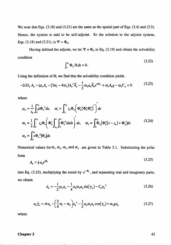
We note that Eqs. (3.18) and (3.21) are the same as the spatial part ofEqs. (3.4) and (3.5).

Hence, the system is said to be self-adjoint. So the solution to the adjoint system,

Eqs. (3.18) and (3.21), is 'II = <I>n.

Having defined the adjoint, we let 'II = <I>n in Eq. (3.19) and obtain the solvability

condition (3.22)

Using the defmition of H, we find that the solvability condition yields

. . ( ) 2- 1 - idI' (3.23) -21 D2 A" -1J111A" - 3al - 4a2 A" A" - - a3abA"e 1 + a3A"g - a4r" = 0 2

where ,

11Z

" J111 = - J1<I>,. 2ds, z" 0

a 1 = r Z. <I> • ( <1>= ( <1>: <I>:n tIs

(3.24)

Numerical values foral' a 2 , a3 , and a 4 are given in Table 3.1. Substituting the polar

form (3.25)

into Eq. (3.23), multiplying the result by e -i!J" , and separating real and imaginary parts,

we obtain

(3.26)

(3.27)

where

Chapter 3 42

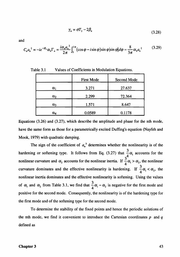
rn = 01"2 - 2/3" (3.28)

and

(3.29)

Table 3.1 Values of Coefficients in Modulation Equations.

First Mode Second Mode

at 3.271 27.637

a2 2.299 72.364

a3 1.571 8.647

a4 0.0589 0.1178

Equations (3.26) and (3.27), which describe the amplitude and phase for the nth mode,

have the same form as those for a parametrically excited Duffing's equation (Nayfeh and

Mook, 1979) with quadratic damping.

The sign of the coefficient of a" 3 determines whether the nonlinearity is of the

hardening or softening type. It follows from Eq. (3.27) that la} accounts for the 4

nonlinear curvature and a2 accounts for the nonlinear inertia. If l al > a2 , the nonlinear 4

curvature dominates and the effective nonlinearity is hardening. If lal < a2 , the 4

nonlinear inertia dominates and the effective nonlinearity is softening. Using the values

of at and a2 from Table 3.1, we find that l at - a2 is negative for the first mode and 4

positive for the second mode. Consequently, the nonlinearity is of the hardening type for

the first mode and of the softening type for the second mode.

To determine the stability of the fixed points and hence the periodic solutions of

the nth mode, we find it convenient to introduce the Cartesian coordinates p and q

defined as

Chapter 3 43

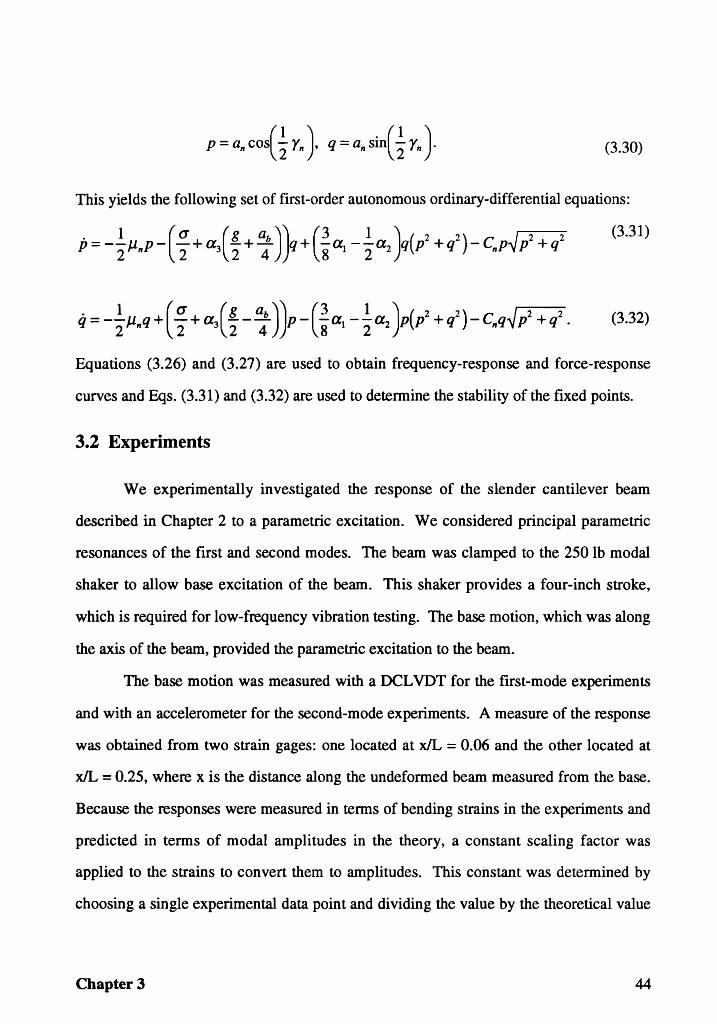
(3.30)

This yields the following set of first-order autonomous ordinary-differential equations:

(3.31)

(3.32)

Equations (3.26) and (3.27) are used to obtain frequency-response and force-response

curves and Eqs. (3.31) and (3.32) are used to determine the stability of the fixed points.

3.2 Experiments

We experimentally investigated the response of the slender cantilever beam

described in Chapter 2 to a parametric excitation. We considered principal parametric

resonances of the first and second modes. The beam was clamped to the 250 lb modal

shaker to allow base excitation of the beam. This shaker provides a four-inch stroke,

which is required for low-frequency vibration testing. The base motion, which was along

the axis of the beam, provided the parametric excitation to the beam.

The base motion was measured with a DCL VDT for the first-mode experiments

and with an accelerometer for the second-mode experiments. A measure of the response

was obtained from two strain gages: one located at xlL = 0.06 and the other located at

xIL = 0.25, where x is the distance along the undeformed beam measured from the base.

Because the responses were measured in terms of bending strains in the experiments and

predicted in terms of modal amplitudes in the theory, a constant scaling factor was

applied to the strains to convert them to amplitudes. This constant was determined by

choosing a single experimental data point and dividing the value by the theoretical value

Chapter 3 44

that corresponds to the same control parameter. This value was then used for all the

experimental data points of that experiment.

The excitation and response signals were monitored with a signal analyzer and an

oscilloscope. For real-time spectral analyses, we used 1280 lines and a Flat Top window.

We used a 10Hz base-band to monitor the response of the first mode and a 20 Hz base­

band to monitor the response of the second mode. The spectra were used to obtain the

contribution of each mode to the response and characterize the observed motion. The

excitation and response spectra were monitored through stationary sweeps of a single

control parameter: either the excitation frequency or the excitation amplitude.

3.3 Results

Here, we compare the results of the theoretical and experimental frequency and

amplitude sweeps. In Fig. 3.1, we theoretical frequency-response curves for the first

mode in the absence of quadratic damping (Le., Cl =0.000) along with experimental

observations. The symbol Z in the figures corresponds to observations obtained during a

reverse sweep and the symbol • corresponds to observations obtained during a forward

sweep in the control parameter. For all the plotted theoretical results, solid lines indicate

stable fixed points and broken lines indicate unstable fixed points. The theoretical

frequency-response curve is bent to the right, indicating that the nonlinear curvature

terms dominate the nonlinear inertia terms for this mode. Also the two theoretical

branches in Fig. 3.1 never close as the excitation frequency is increased. The

experimental frequency-response curve is also slightly bent to the right. The

experimentally obtained response is obviously bounded and does not show any overhang.

There is some qualitative agreement between the experimental and theoretical results

with both curves being bent to the right.

Chapter 3 45

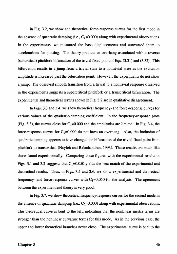
In Fig. 3.2, we show and theoretical force-response curves for the first mode in

the absence of quadratic damping (i.e., Cl=O.OOO) along with experimental observations.

In the experiments, we measured the base displacements and converted them to

accelerations for plotting. The theory predicts an overhang associated with a reverse

(subcritical) pitchfork bifurcation of the trivial fIXed point of Eqs. (3.31) and (3.32). This

bifurcation results in a jump from a trivial state to a nontrivial state as the excitation

amplitude is increased past the bifurcation point. However, the experiments do not show

a jump. The observed smooth transition from a trivial to a nontrivial response observed

in the experiments suggests a supercritical pitchfork or a transcritical bifurcation. The

experimental and theoretical results shown in Fig. 3.2 are in qualitative disagreement.

In Figs. 3.3 and 3.4, we show theoretical frequency- and force-response curves for

various values of the quadratic-damping coefficient. In the frequency-response plots

(Fig. 3.3), the curves close for Cl~.OOO and the amplitudes are limited. In Fig. 3.4, the

force-response curves for Cl ~.OOO do not have an overhang. Also, the inclusion of

quadratic damping appears to have changed the bifurcation of the trivial fixed point from

pitchfork to transcritical (Nayfeh and Balachandran, 1993). These results are much like

those found experimentally. Comparing these figures with the experimental results in

Figs. 3.1 and 3.2 suggests that C1 =0.050 yields the best match of the experimental and

theoretical results. Thus, in Figs. 3.5 and 3.6, we show experimental and theoretical

frequency- and force-response curves with C1=0.050 for the analysis. The agreement

between the experiment and theory is very good.

In Fig. 3.7, we show theoretical frequency-response curves for the second mode in

the absence of quadratic damping (i.e., C2=O.OOO) along with experimental observations.

The theoretical curve is bent to the left, indicating that the nonlinear inertia terms are

stronger than the nonlinear curvature terms for this mode. As in the previous case, the

upper and lower theoretical branches never close. The experimental curve is bent to the

Chapter 3 46

left with a definite overhang. The experimental response jumps from a large amplitude

solution to a trivial solution at 11.07 Hz, whereas the theory predicts that the response

continues to grow as the frequency is reduced. In Fig. 3.8, we show the theoretical force­

response curves for the second mode in the absence of quadratic damping (Le., C2=O.OOO)

along with experimental observations. They agree very well except that during the

reverse sweep in excitation amplitude the observed response jumps down to a trivial

response at ab = 221. 7 inlsecl\2 whereas the predicted response jumps down to a trivial

response at ab = 130.0 inlsecl\2 .

In Figs. 3.9 and 3.10, we show theoretical frequency- and force-response curves

for various values of the quadratic-damping coefficient. As in the previous case, the

frequency-response curves close for C2~0.000. Above a certain value of C2, the

frequency-response curve is stable throughout. In Fig. 3.10, as C2 is increased, the

turning points occur at higher excitation amplitudes. The inclusion of quadratic damping

in the model for the second mode does not change the bifurcation of the trivial response

from pitchfork to transcritical as much as it did for the frrst mode.

In Figs. 3.11 and 3.12, we show and theoretical frequency- and force-response

curves with C2=0.loo for the analysis along with corresponding experimental

observations respectively. As with the previous case, we tried to choose C2 to produce

the best match of the experimental and theoretical results. For this case, we chose C2

such that the excitation amplitude at which the large-amplitude response jumps down to

the trivial response match in the theoretical and experimental frequency-response curves.

However, for this value of C2 the location of the jump in the force-response curves does

not match. The value C2=O.loo is a compromise between matching the locations of the

jumps from the large-amplitude solution to the trivial solution in the frequency- and

force-response curves.

Chapter 3 47

3.4 Discussion and Conclusions

We conducted an experimental and theoretical investigation into the single-mode

responses of a parametrically excited cantilever beam. During excitation of the first

mode, we found a hardening-type frequency-response curve. This experimentally verifies

that, for the first mode, the often ignored nonlinear curvature terms are stronger than the

nonlinear inertia terms. Adding quadr~tic damp'ill~ in the analysis improves the

agreement between the experimental and theoretical results for both the frequency- and

force-response curves of the first mode.

During excitation of the second mode, we found softening-type frequency­

response curves, in agreement with the analysis. The addition of quadratic damping to

the model improves the agreement between the experimental and theoretical results some

what but not nearly as much as for the first mode. This indicates that it may be necessary

to consider different nonlinear damping terms for different modes.

Chapter 3 48

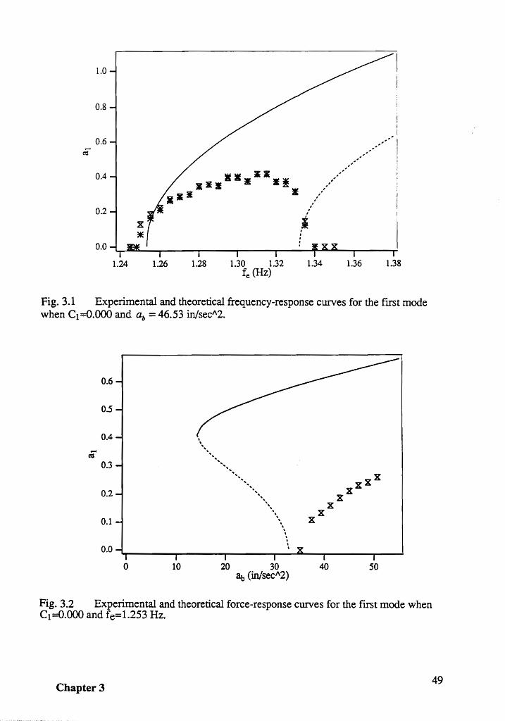
1.0

0.8

0.6 ~

0.4

0.2

0.0

1.24 1.26 1.28 1.30 1.32 fe (Hz)

//././// ...... .

,I , , ,

1.34 1.36

-'

1.38

Fig. 3.1 Experimental and theoretical frequency-response curves for the fIrst mode when Cl=O'OOO and ab =46.53 in/secI\2.

0.6

0.5

0.4

0.3

0.2

0.1

0.0

o 10 20 30 40 50 8t, (in/secI\2)

Fig. 3.2 Experimental and theoretical force-response curves for the firSt mode when Cl=O.OOO and fe=1.253 Hz.

Chapter 3 49

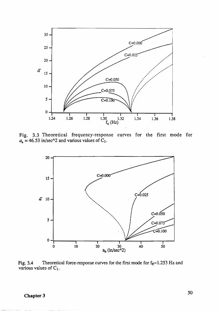
30

25

20

;; 15

10

5

0

1.24 1.26 1.28 1.30 1.32 1.34 1.36 1.38 fe (Hz)

Fig. 3.3 Theoretical frequency-response curves for the first mode for ab = 46.53 in/sec"2 and various values of Cl -

20

15

;; 10

5

C=O.OOO

~ , '.. .. ....

.......... ............

.... .........

'. \

\

'\ , • •

C=O.025

~ O~--____ ~ ______ ~ ______ ~ ____________ ~ __ __

o 10 20 30 40 50 8.t, (in/sec"2)

Fig. 3.4 Theoretical force-response curves for the frrst mode for fe= 1.253 Hz and various values of C l -

Chapter 3 50

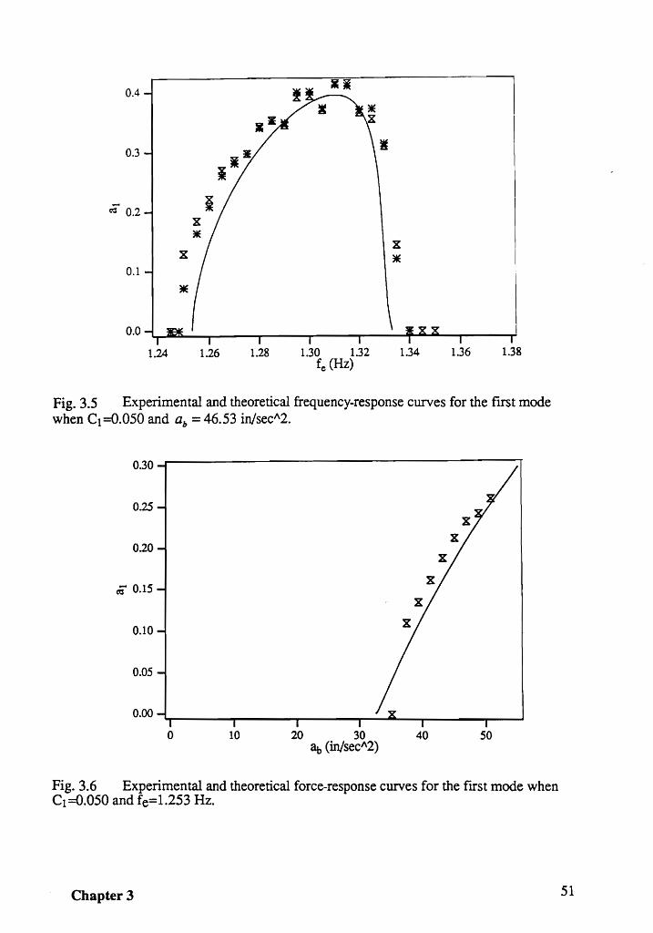
0.4

0.3

~ 0.2

0.1

0.0

1.24 1.26 1.28 1.30 1.32 1.34 1.36 1.38 fe (Hz)

Fig. 3.5 Experimental and theoretical frequency-response curves for the ftrst mode when Cl =0.050 and ab = 46.53 in/sec"2.

0.30

0.25

0.20

~ 0.15

0.10

0.05

0.00

0 10 20 30 40 50 8.f> (in/sec"2)

Fig. 3.6 Experimental and theoretical force-response curves for the frrst mode when Cl =0.050 and fe=1.253 Hz.

Chapter 3 51

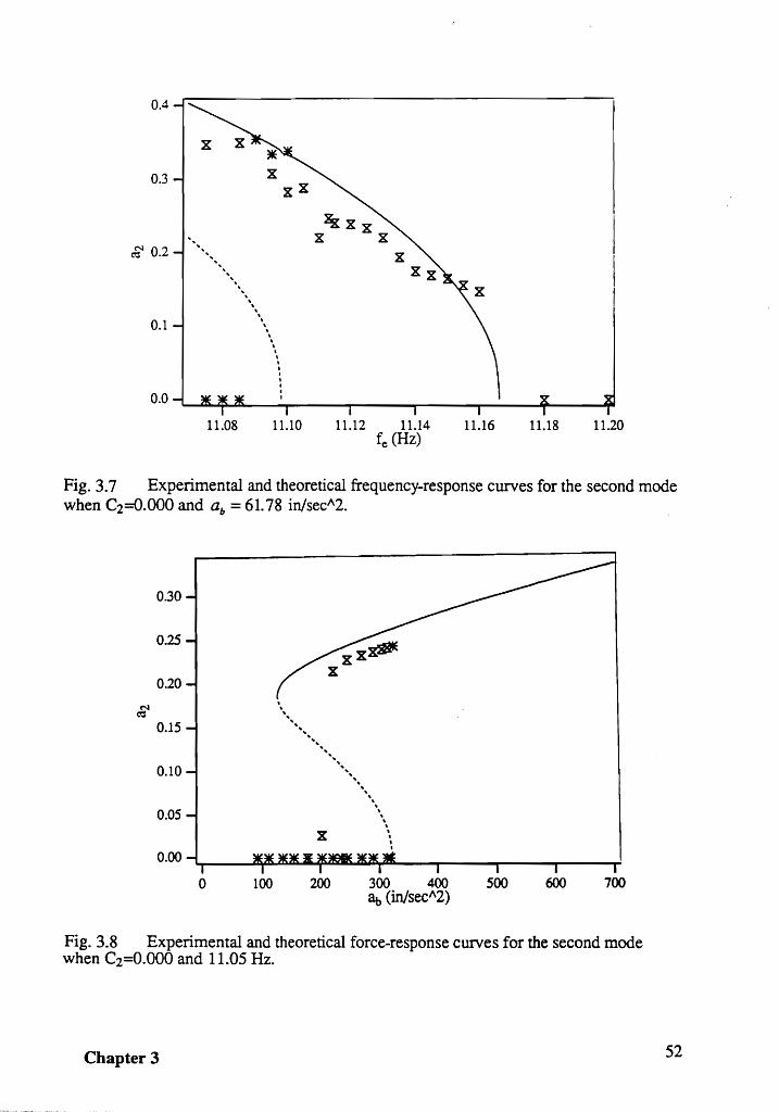
0.4

0.3

~ 0.2 ..

0.1

0.0

.. .. .. .. .. .. .. ..

11.08

.. .. .. , .. .. , \ , .. .. .. .. .. .. , , · I · · I

11.10 11.12 11.14 11.16 11.18 11.20 fe (Hz)

Fig. 3.7 Experimental and theoretical frequency-response curves for the second mode when C2=O'OOO and ab = 61. 78 in/secI\2.

0.30

0.25

0.20

N ec:s

0.15

0.10

0.05

0.00

0 100 200 300 400 ~ (in/secI\2)

500 600 700

Fig. 3.8 Experimental and theoretical force-response curves for the second mode when C2=O'000 and 11.05 Hz.

Chapter 3 52

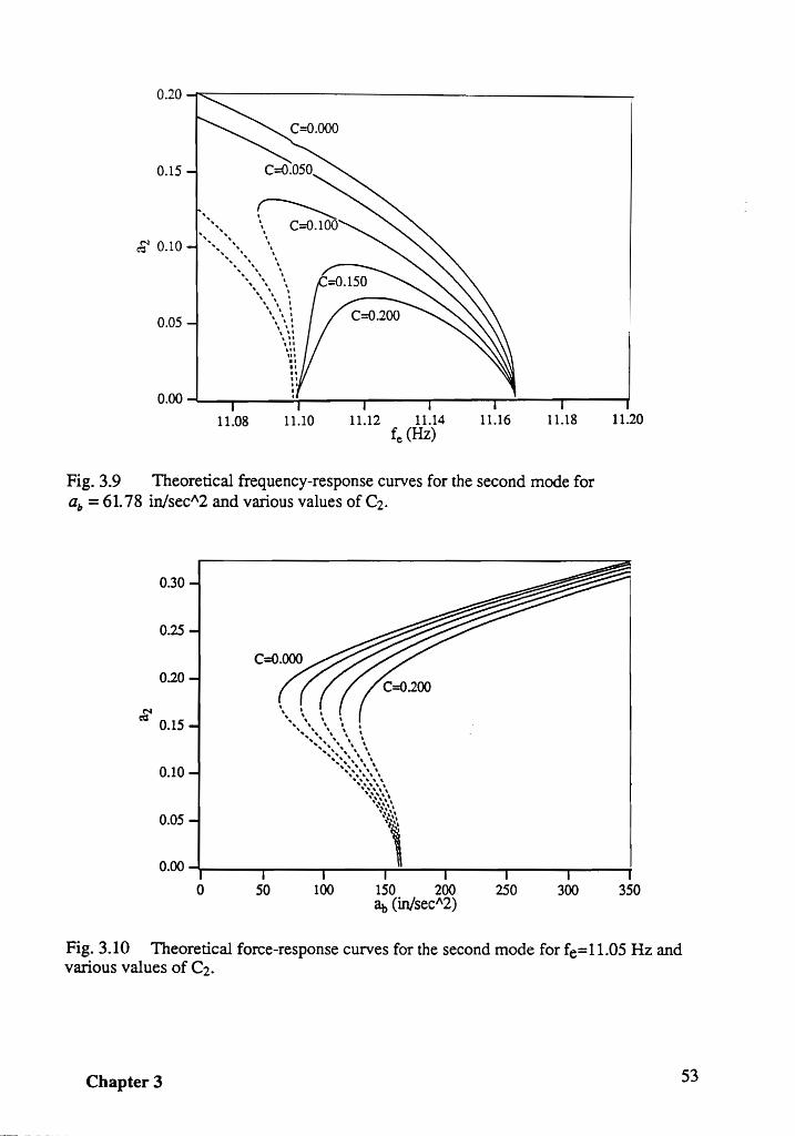
0.20 -r::;::-----------------------..

0.15

~ 0.10

0.05

0.00 -L-_--.!!r-----,-----,.-----,.---:.--r-------r

11.08 11.10 11.12 11.14 11.16 11.18 fe (Hz)

Fig. 3.9 Theoretical frequency-response curves for the second mode for ab = 61. 78 in/secA2 and various values of C2.

0.30

0.25

0.20

N

ed 0.15

0.10

0.05

0.00

0 50 100 150 200 ~ (in/sec"2)

250 300

11.20

350

Fig. 3.10 Theoretical force-response curves for the second mode for fe= 11.05 Hz and various values of C2.

Chapter 3 53

0.35

0.30

0.15

£' 0.10 l 0.!5l

0.10

0.05

O.CO

11.08

. . . . , . , . , . I .

11.10

x XXX

11.12 11.14 fc (HZ)

Xx

11.16 11.18 1

1120

Fi g. 3.11 Experimental and theoretical frequency .. response curves for the second mode when C2=O.100 and a" = 61.78 in/secA2.

0.30

0.25

0.20

M :::

0.15

0.10

0.05

0.00

0 100

. . . . " ~ " " ~

" " " " .. " ~ .. .. .. .. . . , , ,

x: ~

200

. . 300 400 3.t, (in/secA2)

500 600 700

. Fi g. 3.12 Experimental and theoretical force·response curves for the second mode when Cz=O.lOO and fe=11.05 Hz.

Chapter 3 54

4. Experimental Observations of the Transfer of Energy From High-Frequency Excitations to Low­Frequency Response Components

Aeronautical and mechanical systems often have energy inputs at frequencies

much higher than many of their natural frequencies. Examples of such systems include

the space station, by virtue of its very low natural frequencies, and systems with sensitive

instruments isolated from high-frequency noise. If nonlinearities exist in such systems,

the response can be complicated due to nonlinear (modal) interactions. We chose the

flexible cantilever beam described in Chapter 2 as a convenient structure to exhibit some

of these complicated phenomena in a controlled laboratory setting. In such a structure,

modes with frequencies an order of magnitude higher than the frequencies of the first few

modes can be excited. Energy from the directly excited high-frequency modes can be

transferred to low-frequency modes through nonlinear interactions.

In this chapter, we present the results of experimental investigations into the

transfer of energy from high-frequency excitations to low-frequency components in the

response of the flexible cantilever beam. Four cases were considered, three with periodic

base motions along the axis of the beam, and one with a band-limited random base

motion transverse to the axis of the beam. A transfer of energy from high-frequency

modes of the system to low-frequency modes of the system was observed in all four

cases. For the three cases with periodic excitation, the frequency relationship between

the excitation frequency and the lowest frequency component in the response is in the

ratio of 50:1 in two cases and 25:1 in another case. When one or more of the first few

modes are indirectly excited through nonlinear interactions with the directly excited

modes, their motion occurs on a slow-time scale in comparison to the time scale

associated with the motion of the directly excited modes.

55

In the first case, we excited the beam at fe=2f3 with the base excitation at ab=O.85

grms where g is the acceleration due to gravity. In this case, the response remained

planar throughout the frequency sweep. During part of a frequency sweep, a large

response of the first mode was observed. In the second case, we excited the beam at

fe=2f3 with the base excitation at ab=1.41 grms. In this case, the planar motion of the

beam lost stability and large out-of-plane motions were observed. A large response of the

first mode was observed prior to the out-of-plane motion. In the third section, we present

the results of two different experiments. One for fe=138 Hz and ab=0.52 grms, and

another for fe=144.5 Hz and ab=O.52 grms. In these two experiments, the second mode

with a natural frequency of 5.684 Hz dominated the response. It appeared that the shaker

was interacting with the structure. We did not investigate the fe=138 Hz and fe=144.5 Hz

motions in detail but, we present these results to show additional examples of the transfer

of energy from a high-frequency input to low-frequency components in the response.

4.1 Test Description

The test setups used to conduct the experiments with periodic excitations are

described in Chapter 2. For the fe=2f3 case, we conducted stationary frequency sweeps

and monitored the accelerometer and strain-gage spectra. The excitation level was held

constant during the stationary sweeps. We started the experiment at a selected excitation

frequency. Then, at each fe, we waited long enough until a steady-state motion was

achieved, recorded the data, incremented the frequency by a small amount, and repeated

the process. We used Poincare sections and frequency spectra to ascertain if a response

had achieved a steady state. For real-time spectral analyses, we used 1280 lines of

resolution in a 40 Hz baseband and a flat top window.

The test set up for the random excitation was much like that for periodic

excitations except that the beam was mounted on a 100 Ib shaker such that the base

Chapter 4 56

motion was transverse to the axis of the beam. Also, the signal was generated using a

random noise generator and band-pass filtered before it was fed to the shaker amplifier.

During the random excitation, the strain-gage signals were low-pass filtered through a

six-pole elliptic filter with a cut-off frequency of 50 Hz. For spectral analyses, we used

1280 lines of resolution in a 40 Hz baseband, a Hanning window, and 30 overlap

averages.

For the fe=138 Hz case, we obtained the accelerometer and strain-gage spectra for

a single excitation amplitude and frequency. For real-time spectral analyses, we used

1280 lines of resolution in a 160 Hz baseband and a flat top window.

To calculate the pointwise dimension (Moon, 1987), and high resolution FFT, we

collected 72,000 points from the base strain-gage at a sampling frequency of 120.0 Hz.

This was done for selected motions. The signal was low-passed filtered with a cut-off

frequency of 50 Hz before data acquisition. For the dimension calculations we used 1000

reference points. For the high resolution FFT's, 65536 (216) points were used with a

Kaiser window.

Throughout this discussion, we refer to the frequency component of the response

near a natural frequency of a particular mode as that particular mode's contribution to the

response. For large motions, this assumption may be questionable due to the possible

presence of harmonics of certain frequency components and peaks at combinations of the

frequency components. In the experiments, the mode shapes corresponding to the largest

components of the forced response could be visually identified by the nurnber of nodes.

In addition, for the case discussed below where the third mode was initially the largest

contributor to the response, the mode shape was measured. This was done by measuring

the displacements optically at different locations along the beam while the excitation

parameters were held constant. The amplitude of the third mode was measured from the

peak near f3 in the response spectrum. These values were plotted against the location

Chapter 4 57

along the beam and compared to the linear mode shape obtained from the Euler-Bernoulli

beam theory. They matched very closely. This indicates that, for this case, a peak in the

spectrum near a natural frequency corresponds to that particular mode.

4.2 Planar Motion for fe ::::: 2f3

The excitation frequency was varied between 33.00 Hz and 30.90 Hz while the

base acceleration was held constant at 0.85 gs rms. In Fig. 4.1a, the ranges of fe in which

the different responses occur in terms of the participating modes are summarized. Note

that, throughout the considered range of fe, two different responses were found for each

frequency setting except between 32.2 Hz and 32.73 Hz where only one response was

found. In Fig. 4.1 b, the frequency-response curve obtained during a downward sweep in

frequency is presented. In Fig. 4.1 c, the frequency-response curve obtained during an

upward sweep in frequency is presented. In Fig. 4.1 the amplitudes correspond to the

root sum squared (rms) of the signal at each modes response frequency. The scale for

Fig. 4.1c was chosen to highlight the fourth mode's response. In Figs. 4.1 band 4.1c, an

approximate conversion from strains to relative displacements was made by multiplying

each mode's contribution to the response by fi/f3, where fi is the natural frequency of the

ith mode. This conversion gives a better measure of the displacements observed during

the experiment.

We observed a combination resonance involving the first and fourth modes when

fe was between 33.00 Hz and 32.74 Hz during the downward sweep. A typical spectrum

of this type of response is shown in Fig. 4.2a. The sum of the frequencies of the

responses of the first and fourth modes is equal to the excitation frequency. A peak at the

excitation frequency is also present. By using a time delay of 0.33 seconds, we

calculated the pointwise dimension for this motion to be about 2.0 for n=10. The points

in the Poincare section, shown in Fig. 4.2a, form a closed loop. Both these tools indicate

Cbapter4 58

that the motion is a two-period quasi-periodic motion in agreement with the spectrum.

This response was difficult to obtain because very few initial conditions led to this

motion. Many tries of "tapping" the beam to give different initial conditions were

required to obtain this motion. The response, which most of the initial conditions would

evolve to, had a single peak in the spectrum at the excitation frequency.

A response due to a principal parametric resonance of the third mode and a

primary external resonance of the fourth mode was observed for fe between 32.74 Hz and

32.40 Hz in both the downward and upward frequency sweeps. The frequency of the

response of the third mode was fel2 and the frequency of the response of the fourth mode

was fe. A spectrum of this type of response is shown in Fig. 4.2b. The third mode

component dominated the response, as seen in Figs. 4.1b and 4.1c. Using 72000 points,

1000 reference points, and a time delay of 0.33 seconds, we calculated the pointwise

dimension for this motion to be about 1.0 for n=10. The Poincare section, shown in

Fig. 4.2b, consists of two discrete points. Both the Poincare section and the dimension

indicate a periodic motion. The two points in the Poincare section and the spectral line at

fel2 indicate that the motion had a basic period twice that of the excitation period.

A three-mode response that included the first mode was first observed at

approximately 32.4 Hz during the sweep down in fe. The three-mode response continued

as the frequency was swept down until 30.10 Hz, where the first and third modes dropped

out of the response, resulting in only a small peak at fe in the spectrum. As the frequency

was swept up, a transition from the single fourth-mode response to a three-mode response

occurred at 32.19 Hz. A spectrum of the three-mode response, when the first mode

component was large, is shown in Fig.4.2c. When the three-mode response was

observed, there were sidebands about the fel2 peak in the spectrum. The difference in

frequency fm between the fe/2 peak: and the sidebands varied throughout the frequency

sweep. The frequency of the first-mode component of the response was equal to fro. In

Chapter 4 59

the excitation frequency range between 32.22 Hz and 32.19 Hz, fm was approximately

0.65 Hz, which is close to the natural frequency of the first mode. This resulted in a

response with a large first-mode component, as shown in Figs. 4.1b and 4.1c. The

spectrum has discrete lines with fm and fe being the discernible incommensurate

frequencies. Generating the Poincare section for this motion, we found that the points

generated two small loops, as shown in Fig. 4.2c. The length of time to collect the 512

points for the Poincare section was about 16.0 seconds. The spectrum and the Poincare

section indicate a two-period quasi-periodic motion in the time span considered.

However, the first-mode component of the spectrum never settled down to a constant

value even after a long time (30 minutes). The pointwise dimension was about 2.25 for a

delay of 0.33 seconds at n=10. These results indicate a basic two-period motion that is

chaotically modulated. During the three-mode response, we measured a static component

in the strain, which returned to zero when the three-mode response was not present. We

measured the static displacement of a node of the third mode and observed that it changed

as we changed fee The analysis of Chapter 5 helps us interpret this response as a static

response of the first mode due to a dynamic response of the third and fourth modes.

A response consisting of the fourth mode alone was observed for most of the

upward frequency sweep, as shown in Fig. 4.1c. A jump in the response, characteristic of

a forced Duffing's oscillator with a softening spring, was observed. The Poincare section

for this motion consisted of a single point, the dimension was about 1.00, and the

spectrum had a single peak. These results indicate a periodic motion with a basic

frequency equal to the excitation frequency. During the downward frequency sweeps,

besides the fourth mode, the third mode was present in the response. Although the fourth

mode was excited by a primary resonance, the expected increase in amplitude of the

fourth mode did not occur. This can be seen in Fig. 4.1 b. During the upward frequency

sweeps, the increase in amplitude of the fourth mode can be seen in Fig. 4.1c. When the

Chapter 4 60

third mode appeared at 32.4 Hz during the upward frequency sweep, the amplitude of the

fourth mode decreased as seen in Fig. 4.1c. This suggests that the presence of the third

mode suppressed the fourth mode.

4.3 Out-of-Plane Motion for fe ::= 2f3

For this experiment, the excitation frequency was varied between 32.000 Hz and

31.877 Hz while the base acceleration was held constant at ab=1.414 grms. During a

downward sweep in frequency a planar three-mode motion similar to that discussed in the

previous section loses stability and an out-of-plane motion occurs. In this section, we

focus on the transition from the planar to out-of-plane motion and characterize the out-of­

plane motion. This transition only occurred during a downward frequency sweep.

Cusumano (1990) investigated similar out-of-plane motions of a flexible cantilever beam

subjected to an external excitation.

A response due to a principal parametric resonance of the third mode and a

primary external resonance of the fourth mode was observed at fe=32.000 Hz in a

downward frequency sweep. The frequency of the response of the third mode was fel2

and the frequency of the response of the fourth mode was fee Spectra of this type of

response and the associated base acceleration are shown in Fig. 4.3. This spectrum of the

base acceleration is typical of the rest of the experiment so the others are not shown. As

the frequency was reduced to 31.880 Hz, the first mode came into the response along

with sidebands about the fel2 and fe peaks in the spectrum, as shown in Fig. 4.4. This

motion has essentially the same characteristics as the three-mode motion discussed in the

previous section.

As the excitation frequency was reduced to fe=31.879 Hz, an increase in the

magnitude and number of sidebands about fe and fel2 peaks occurred, as shown in Fig.

4.5. This corresponds to an increase in the amplitude of the modulations. In addition, an

Chapter 4 61

increase in the magnitude of the peak associated with the first mode occurred. A time

history of a strain-gage signal for this type of motion is shown in Fig. 4.6. The

oscillations of the envelope correspond to the sidebands in the spectrum.

As the excitation frequency was reduced to fe=31.878 Hz, additional sidebands

were observed. A zoom span spectrum from 10Hz to 20 Hz around the fel2 peak with

1280 lines of resolution is shown in Fig. 4.7. The peaks appear to be spread over several

lines of resolution indicating that the response may be chaotic. Unfortunately, we did not

obtain a long time history for this motion for post-experiment calculation of the

dimension.

As the excitation frequency was reduced to fe=31.877 Hz, we visually observed a

slow increase of the amplitude of the first mode. After some time, the planar motion lost

stability and a large out-of-plane motion was observed. A spectrum of the out-of-plane

motion is shown in Fig. 4.8. We note that the response has a broadband spectrum. A

Poincare section of this motion is shown in Fig. 4.9. The Poincare section does not have

a simple geometry such as a point, line, or loop; thus, the long term motion is referred to

as a strange attractor. The dimension dp was found to be about 5.26. All the tools used to

characterize this motion indicate that the motion is chaotic. A time history of a strain­

gage signal for this motion as the beam transitioned from a planar to an out-of-plane

motion is shown in Fig. 4.1 O. We point out the abrupt change from a response dominated

by high-frequency components to one dominated by a low-frequency component.

4.4 Band-Limited Random Base Excitation

To investigate if nonlinear interactions occur with a band-limited random base

excitation, we conducted another experiment. For this case, the beam was excited by

random excitation in the frequency range from 10Hz to 50 Hz to preclude a direct

excitation of the first and second modes through linear mechanisms. The excitation

Chapter 4 62

signal was high-pass filtered through a six-pole elliptic filter with a cut-off frequency of

10 Hz and subsequently low-pass filtered through a six-pole elliptic filter with a cut-off

frequency of 50 Hz.

The spectra of the response and the excitation are shown in Fig. 4.11 Although

the beam was not provided with any input energy for frequencies less than 10 Hz, the

output spectrum still contains peaks near the first and second natural frequencies besides

peaks near the third and fourth natural frequencies. This observation indicates that the

first and second modes are excited through nonlinear mechanisms. The first and second

modes may be either indirectly excited by an energy transfer from the third and fourth

modes, as in the previous case, or directly excited through combination resonances.

4.5 Periodic Base Excitation: fe = 138 Hz and fe=144.0 Hz

Two additional tests were conducted to determine if the transfer of energy from

high-frequency modes to a low-frequency mode is an isolated phenomenon or if it occurs

for a variety of conditions. The test setup used was the same as that used for the fe=2f3

case. The excitation frequency fe was 138 Hz for one test and 144 Hz for the other with a

base acceleration ab=O.52 grms for both. The 138 Hz frequency is near the eighth natural

frequency of the beam, where as the 144 Hz is not near any natural frequencies of the

beam.

The strain-gage and the base acceleration spectra for fe=138 Hz are shown in

Fig. 4.12. In the strain-gage spectrum, there is a large peak near 5.6 Hz and two small

peaks near the excitation frequency that are separated by approximately 5.6 Hz. A visual

inspection indicated that the response of the beam was clearly dominated by the second

mode. The two high-frequency peaks in the response spectrum are less than a tenth of the

magnitude of the low-frequency peak. Also, note that the measured response is the strain.

A conversion that approximately converts from strains to relative displacements is

Chapter 4 63

f2/f8=O.04, where f8 is the natural frequency of the eighth mode. This indicates that the

response of the second mode is approximately 250 times the high-frequency components

in the response. Arguably, the high-frequency components in the strain-gage spectrum

are negligible. The base acceleration spectrum has a main peak at 138 Hz, which is the

frequency of the signal from the signal generator. There are also large sidebands around

138 Hz in the acceleration spectrum, indicating that the base acceleration is modulated.

As in the first case, the frequency difference between the carrier frequency and the

sidebands is near the natural frequency of a low-frequency mode of the beam. In this

case, modulations are seen in the base motion.

In Fig. 4.13, we show the spectra of the base strain gage signal and the base

accelerometer signal for fe=I44.0 Hz and ab=O.52 grms. There are multiples of 60 Hz in

the response spectrum that are due to line noise and should be ignored. Again, there is a

large second-mode contribution to the response. As in the previous case, there are

sidebands in the acceleration spectrum, indicating modulations of the base acceleration.

In addition, there are small peaks in the strain-gage spectrum at the same frequencies as

in the acceleration spectrum. The spacing fm of the high-frequency peaks is equal to the

response frequency of the second mode. This indicates that an interaction occurred

between the complete response of the low-frequency second mode and the modulations of

the high-frequency components in the experiment.

There are two interpretations of the low-frequency single-mode responses with a

modulated input that were observed. One is that the response consists of essentially a

single low-frequency mode excited by a modulated input. The other one is that the

response consists of two modes with one being the low-frequency second bending beam

mode and the other including the shaker system. This multi-mode response is driven by

the periodic signal from the signal generator.

Chapter 4 64

4.6 Concluding Remarks

In the experiments with fe=2f3, the nonlinear mechanism responsible for exciting

the first mode involved an energy exchange between the complete response of the first

mode and the modulations associated with the high-frequency third and fourth modes.

This resonance is a distinctly different mechanism than the combination resonance for

transferring energy from a high-frequency excitation to a low-frequency mode (Dugundji

and Mukhopadhyay, 1973). In the case of the cantilever beam, this type of transfer of

energy was found to be robust and occurred for a variety of excitations. Such transfer of

energy is expected to occur in other structures as well.

In addition, in the fe=2f3 experiments, a variety of resonant responses were

observed in a small range of the excitation frequency. These results highlight the

richness of the response of a simple structure. They also point out some of the difficulties

that can be encountered in predicting the response of a nonlinear continuous structure due

to the many nonlinear resonances.

The experiments conducted on the cantilever beam were at the same time "good

experiments" and "bad experiments". They were good because they revealed a

previously unstudied modal interaction. The understanding of the phenomena gained

from the experiments guided an analysis that captures the unusual characteristics of the

observed motions. The analysis is presented in Chapter 5. The results from these studies

could have applications to other flexible structures. Because of this, the experiments

were part of a significant contribution to the art and science of engineering. At the same

time, 'the experiments were "bad" because they were not very repeatable. With repeated

experiments, the same type of motions would be observed but, the excitation levels and

frequencies required for the various motions would change. This was due primarily to

the beam yielding during the experiments. The motion that did the most damage was the

Chapter 4 65

out-of-plane motion. This unfortunately was the favorite motion to show visitors. In

hindsight, this type of motion should have been kept at a minimum. The result of this

nonrepeatability was to make it difficult to obtain experimental results, analyze them, and

go back and try and obtain more results at the same settings of the control parameter to

characterize the motion further.

Chapter 4 66

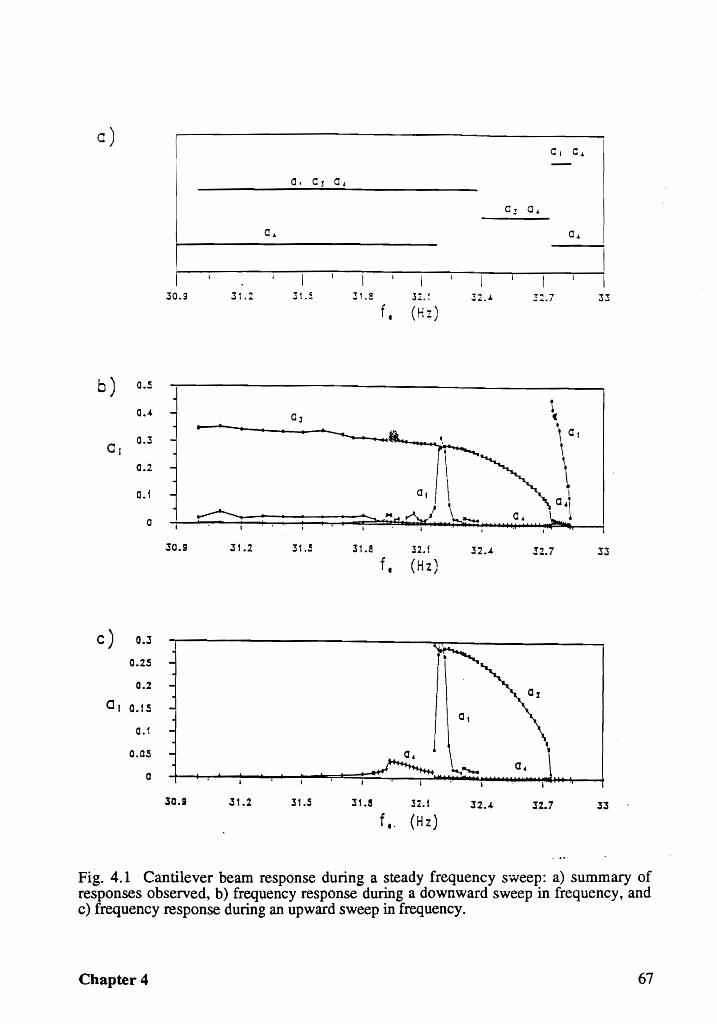
a)

30.9 31.2 31.: 31.1 32 • .4 !2.7

f. (Hz)

b) O.S

~ •

0 ..... ~

OJ « - .. • . .... ~ . , 0 t

0, 0.3

1 ~ . ,

0.2 \ ~o\ Q. f

0 \ -.-. o. I '1

30.9 31.2 31.S 31.8 .'52. f 32 ..... .!2.7 33

f. (H z)

c) 0.3

Q.25

0.2

01 O. f 5

0.1

~a, 0, \

0.05

a

.30.1 .31.2 31.S 31.8 32.1 32 ..... 32.7 33

f •. (Hz)

Fig. 4.1 Cantilever beam response during a steady frequency sweep: a) summary of responses observed, b) frequency response during a downward sweep in frequency, and c) frequency response during an upward sweep in frequency.

Chapter 4 67

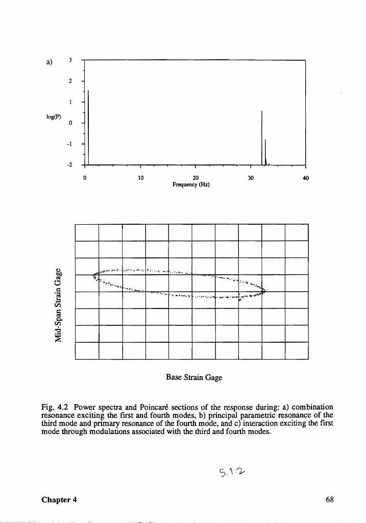
a) 3

-2 -

--

log(P) 0 -

-1 -.

-2 I I I

0 10 20 30 40 Frequency (Hz)

~,ta rdJt ............. r . " ....... , - ......... ... I .. i .. " .. I. _.. .. .. _ .... _ _ " ..

':1-_'-... ................. -'-.a-. .

.. ..... , ........... .. • .. r

........ - ...... -., • •• : ......................... tt. ... -: ... .........

Base Strain Gage

Fig. 4.2 Power spectra and Poincare sections of the response during: a) combination resonance exciting the first and fourth modes, b) principal parametric resonance of the third mode and primary resonance of the fourth mode, and c) interaction exciting the first mode through modulations associated with the third and fourth modes.

Chapter 4 68

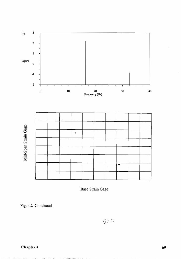
b) 3

2 -

-

log(P) 0 -

·1 -

·2 I I I

0 10 20 30 40 Frequency (Hz)

....

....

Base Strain Gage

Fig. 4.2 Continued.

Chapter 4 69

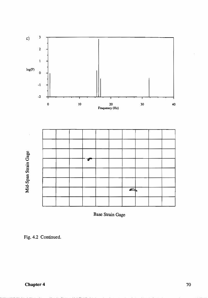
c) 3

2 -

-

log(P) 0 -

·1 -

-2 I I I

0 10 20 30 Fwquency (Hz)

¥~

~ ...

Base Strain Gage

Fig. 4.2 Continued.

Chapter 4 70

BASE STRAIN GAGE

1.000 ~ .

LOG ~

~

~

~

i.000e-05 . 0.0 LIN FREQ (HZ) 40.00

BASE ACCEL. . 10.00 .;; ~

· f-

LOG ~ ~ -:: ..

J :-·

~ 5 · ..

i.000e-03 . . 0.0 LIN FREG (HZ) 40.00

Fig. 4.3 Strain-gage and base acceleration spectra for fe=32.00 Hz and ab=1.414 grms.

o DEG STRAIN GAGE . . . 1.000 J

-= ~

LOG ~ ~ -· ~ ~ · :-

~

~ J. II. ~ · ~

It I U JI .L L II l-1.000e-04

t . t

0.0 LIN FREQ (HZ) 40.00

Fig. 4.4 Strain-gage spectrum for fe=31.880 Hz and aF1.414 grms.

Chapter 4 71

o DEG STRAIN GAGE . , I

1.000 ~

I ~.

~

LOG ~ j ~ · · i ·

J

I ~ : · ·

~

lL.1 ~ -: · dJ._I_. _. IIHI III :

· .1l 1 -- - --- - __ A -.... . T

1.000e-04

0.0 LIN FRED (HZ) 40.00

Fig. 4.5 Strain-gage spectrum for fe=31.879 Hz and alF1.414 grms.

0.3

........... CI1 0.2 .... -oJ 0 > .......,

0.1 LIJ C)

...: C) 0

z ...: a::: -0.1 .... CI1

LIJ -0.2 en

...: CD

-0.3

0 5 10 15 20 25

TIME (SEC)

Fig. 4.6 Time trace of a quasi-periodic motion for fe=31.879 Hz and ab=1.414 grms.

Chapter 4 72

45 OEG STRAIN GAGE

1.000

LOG

1 . OOOe-O 4 -+----+--"t---'---+-LL-.

10.00 LIN FRED (HZ) 20.00

Fig.4.7 Strain-gage zoom span spectrum for fe=31.878 Hz and ab=1.414 grms.

Chapter 4 73

o DEG STRAIN GAGE

0.0 LIN FREQ (HZ) BO.OO

Fig. 4.8 Strain-gage spectrum for fe=31.877 Hz and aLF1.414 grms .

.. '

"

. ' .. .. .. ..

:* ••• ' :. : ... " iIO... .. ..

.. " :

: ' .. . ....... ....

-. .."

... .. -, .. _ .. : ..

...... .. I· •• .. •

...... ":.:. iIO. : •• :_ .... • ..... "

- •• _iIO ...

"

"

..... iIO. . .... :.:

Mid-Span Strain Gage

Fig. 4.9 Poincare section for fe=31.880 Hz and ab=1.414 grms.

Chapter 4 74

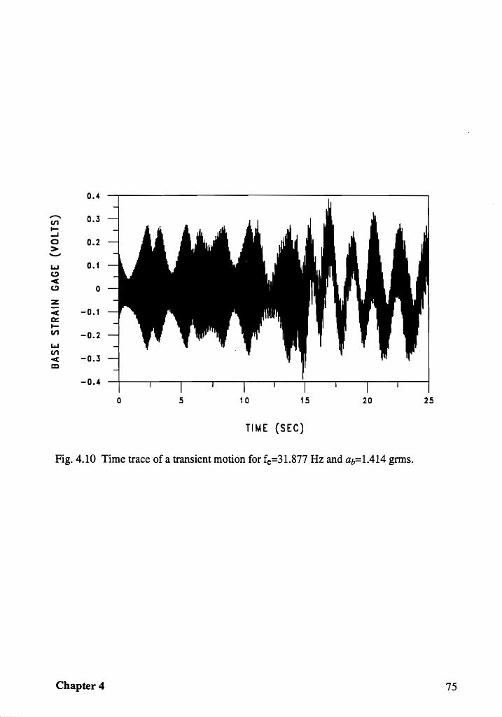
0.4

.......... 0.3 CI1 t-..J 0 0.2 > ....... L&J 0.1 C) 411'( C) 0

z -411'( -0.1 a:: t-CI1 -0.2 Lr.I CI1 411'( -0.3 III

-0.4

0 5 10 15 20 25

TIt.4E (SEC)

Fig. 4.10 Time trace of a transient motion for fe=31.877 Hz and ab=I.414 grms.

Chapter 4 75

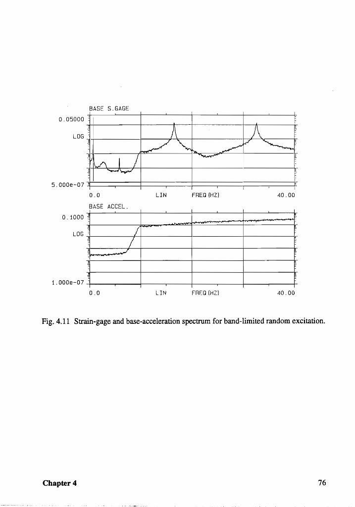
BASE S.GAGE

0.05000 .

LOG

5.000e-07~====;=====~==~=====t====~====1=====~====t 0.0 LIN FREQ (HZ) 40.00

BASE ACCEL.

0.1000 ~ ~

LOG I .... ~

/ ~ ~ ~

.;

~ f i.OOOe-07

0.0 LIN FREQ (HZ) 40.00

Fig. 4.11 Strain-gage and base-acceleration spectrum for band-limited random excitation.

Chapter 4 76

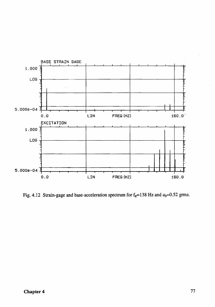
1.000

LOG

5.000e-04

1.000

LOG

5.000e-04

BASE STRAIN GAGE . :: -

,;;

1 :

§ . 0.0

EXCITATION I

.;;

~ : . ::

": .

~ J

0.0

J .

I

I

LIN

I

. . LIN

. , . I , ~. ..

~ ~

~ "!'

I I

I I :: . . I . · FREQ (HZ) 160.0:"

t I . . · ~ !-.

~ "',

~ ....

-I

I I ! . I · FREG (HZ) 160.0

Fig. 4.12 Strain-gage and base-acceleration spectrum for fe=138 Hz and ab=O.52 gnns.

Chapter 4 77

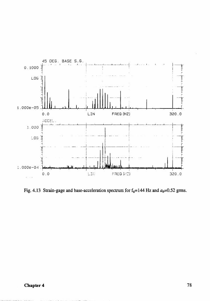
45 OEG. BASE S.G. o . 1000 -t--- I

.1 __ ._j - . I .. I _

J

LOG 1 -~

---t:-

. J 1~llllll-;,-t, I -! ..

I"'

:

1.000e-051111J ""j - -. ~

i j

I. i, I I r I

I i I

0.0 LIN FREQ (HZ) 320.0

Fig. 4.13 Strain-gage and base-acceleration spectrum for fe=l44 Hz and am.52 gnns.

Chapter 4 78

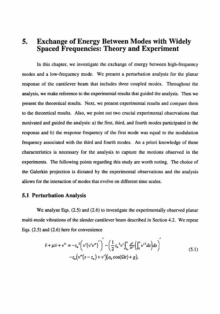
5. Exchange of Energy Between Modes with Widely Spaced Frequencies: Theory and Experiment

In this chapter, we investigate the exchange of energy between high-frequency

modes and a low-frequency mode. We present a perturbation analysis for the planar

response of the cantilever beam that includes three coupled modes. Throughout the

analysis, we make reference to the experimental results that guided the analysis. Then we

present the theoretical results. Next, we present experimental results and compare them

to the theoretical results. Also, we point out two crucial experimental observations that

motivated and guided the analysis: a) the first, third, and fourth modes participated in the

response and b) the response frequency of the first mode was equal to the modulation

frequency associated with the third and fourth modes. An a priori knowledge of these

characteristics is necessary for the analysis to capture the motions observed in the

experiments. The following points regarding this study are worth noting. The choice of

the Galerkin projection is dictated by the experimental observations and the analysis

allows for the interaction of modes that evolve on different time scales.

5.1 Perturbation Analysis

We analyze Eqs. (2.5) and (2.6) to investigate the experimentally observed planar

multi-mode vibrations of the slender cantilever beam described in Section 4.2. We repeat

Eqs. (2.5) and (2.6) here for convenience

I I

V+ ,uv + v;' = -z. 2 ( v'( v'v")') - G z.. V ( ;: (J:V'2 tis)tis )

(5.1)

- z" ( V" (s - z,. ) + V,)( ab cos( Ot ) + g),

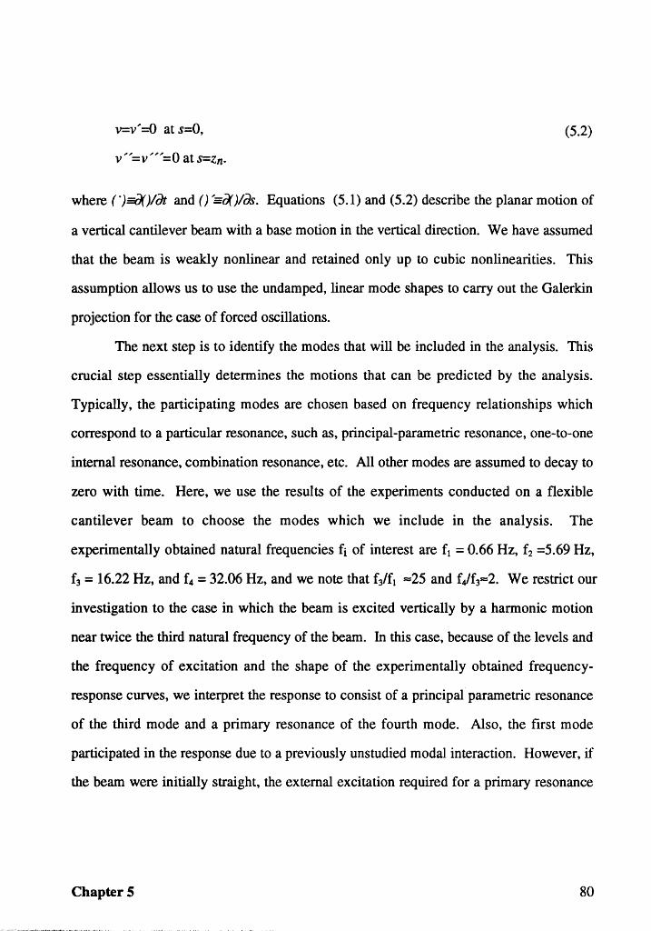
v=v" =0 at s=O,

v"=v"'''=O at s=zn.

(5.2)

where (")=(X)ldt and () "=~)Ias. Equations (5.1) and (5.2) describe the planar motion of

a vertical cantilever beam with a base motion in the vertical direction. We have assumed

that the beam is weakly nonlinear and retained only up to cubic nonlinearities. This

assumption allows us to use the undamped, linear mode shapes to carry out the Galerkin

projection for the case of forced oscillations.

The next step is to identify the modes that will be included in the analysis. This

crucial step essentially determines the motions that can be predicted by the analysis.

Typically, the participating modes are chosen based on frequency relationships which

correspond to a particular resonance, such as, principal-parametric resonance, one-to-one

internal resonance, combination resonance, etc. All other modes are assumed to decay to

zero with time. Here, we use the results of the experiments conducted on a flexible

cantilever beam to choose the modes which we include in the analysis. The

experimentally obtained natural frequencies fi of interest are ft = 0.66 Hz, f2 =5.69 Hz,

f3 = 16.22 Hz, and f4 = 32.06 Hz, and we note that f3/fl =25 and fJf3=2. We restrict our

investigation to the case in which the beam is excited vertically by a harmonic motion

near twice the third natural frequency of the beam. In this case, because of the levels and

the frequency of excitation and the shape of the experimentally obtained frequency­

response curves, we interpret the response to consist of a principal parametric resonance

of the third mode and a primary resonance of the fourth mode. Also, the first mode

participated in the response due to a previously unstudied modal interaction. However, if

the beam were initially straight, the external excitation required for a primary resonance

Chapter 5 80

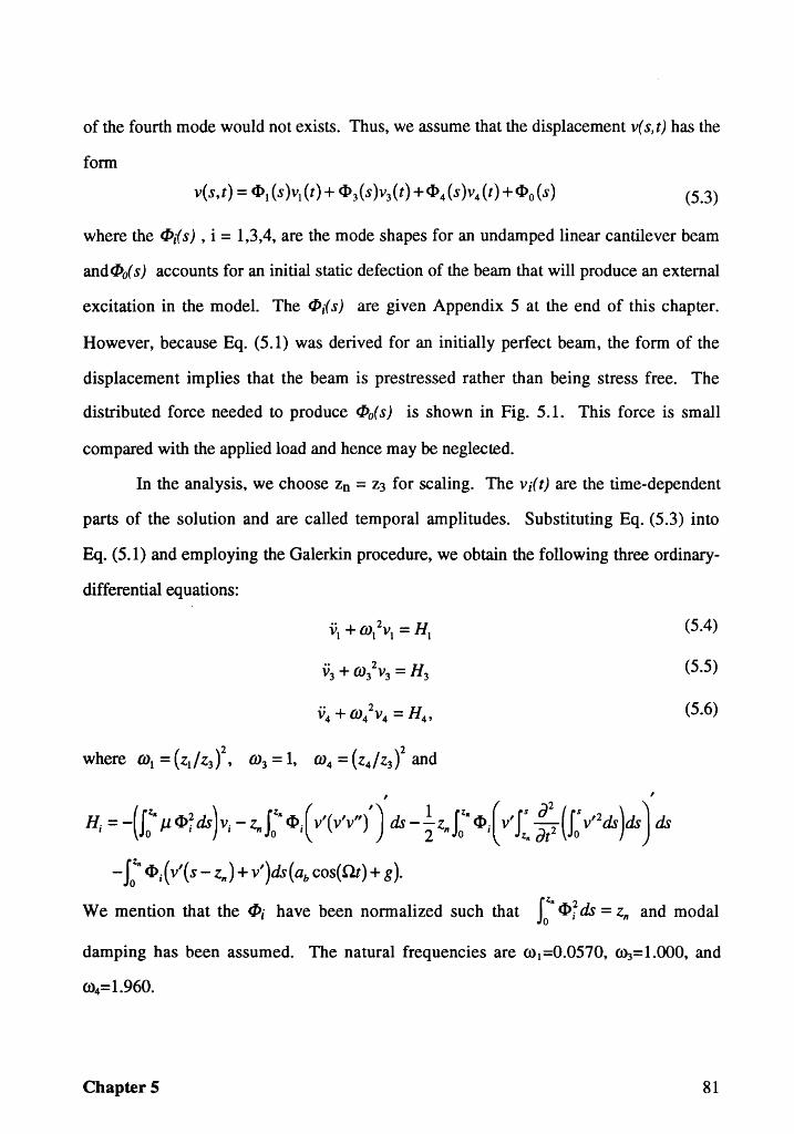
of the fourth mode would not exists. Thus, we assume that the displacement v( s,t) has the

fonn

(5.3)

where the tPls) , i = 1,3,4, are the mode shapes for an undamped linear cantilever beam

andtPo(s) accounts for an initial static defection of the beam that will produce an external

excitation in the model. The tP;(s) are given Appendix 5 at the end of this chapter.

However, because Eq. (5.1) was derived for an initially perfect beam, the form of the

displacement implies that the beam is prestressed rather than being stress free. The

distributed force needed to produce tPo(s) is shown in Fig. 5.1. This force is small

compared with the applied load and hence may be neglected.

In the analysis, we choose Zn = Z3 for scaling. The Vi(t) are the time-dependent

parts of the solution and are called temporal amplitudes. Substituting Eq. (5.3) into

Eq. (5.1) and employing the Galerkin procedure, we obtain the following three ordinary­

differential equations:

I I

Hi = -(Jo'" Jl4>; ds)vi - z.J:" 4>{ V'(v'v"n ds - ~ z.Io" 4>{ v'1:. !22 (J: v'2ds)ds ) ds

-J:" <l> i ( Vi ( S - zn) + v/)ds (ab cos( at ) + g).

(5.4)

(5.5)

(5.6)

illl 2 We mention that the tPi have been normalized such that 0 <l>j ds = Zn and modal

damping has been assumed. The natural frequencies are ffil=O.0570, ~=1.000, and

Chapter 5 81

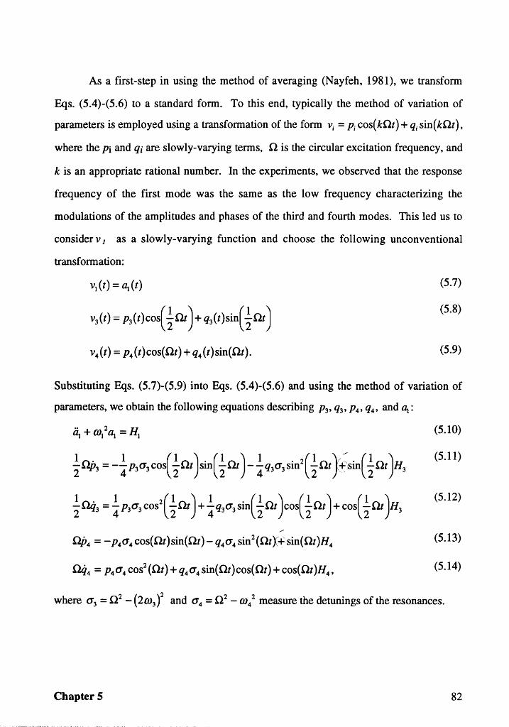
As a first-step in using the method of averaging (Nayfeh, 1981), we transform

Eqs. (5.4)-(5.6) to a standard form. To this end, typically the method of variation of

parameters is employed using a transformation of the form Vi = Pi cos( kat) + qi sin( kat),

where the Pi and qi are slowly-varying terms, a is the circular excitation frequency, and

k is an appropriate rational number. In the experiments, we observed that the response

frequency of the first mode was the same as the low frequency characterizing the

modulations of the amplitudes and phases of the third and fourth modes. This led us to

consider V 1 as a slowly-varying function and choose the following unconventional

transformation:

(5.7)

(5.8)

(5.9)

Substituting Eqs. (5.7)-(5.9) into Eqs. (5.4)-(5.6) and using the method of variation of

parameters, we obtain the following equations describing PJ' qJ' P4' q4' and llt:

/'

np 4 = - P 40'4 cos( at) sin( at) - Q40'4 sin 2 (at X + sin( at )H4

(5.10)

(5.11)

(5.12)

(5.13)

(5.14)

where O'J = 0 2 - (2mJ)2 and 0'4 = 0 2 -m/ measure the detunings of the resonances.

Chapter 5 82

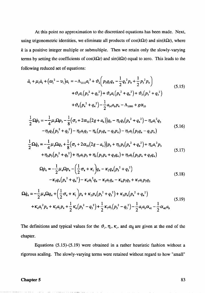
At this point no approximation to the discretized equations has been made. Next,

using trigonometric identities, we eliminate all products of cos(kOt) and sin(kOt), where

k is a positive integer multiple or submultiple. Then we retain only the slowly-varying

terms by setting the coefficients of cos(kQt) and sin(kQt) equal to zero. This leads to the

following reduced set of equations:

•• • (2 ) A 3 A<l ( 1 2 1 2 ) ll:t + J11ll:t + (01 - VI ll:t = - llull:t + U2 P3q3q4 - 2 q3 P4 + '2 P3 P4

+iJ3ll:t(p/ +q/)+ iJ4ll:t(p/ +q/)+ iJ5(p/ +q/)

.!.np3 = -.!.J13Qp) -.!.( 0'3 + 2a33 (2g + ab ))q3 - 112q3(P/ + q/) - 114ll:t 2q3 2 4 8

-113q3(P/ + q/) - 115ll:tq3 - 116 (P3q4 - q3P4) - 117ll:t (P3Q4 - Q3P4)

~ 1lq3 = - ! Jl30lb +~( 0'3 + 2a33(2g -ab )}P3 + ThP3(P/ +q/)+ 1J.a/ P3

+ 113P3 (P32 + Q/) + 11sll:tP3 + 116 (P3P4 + q3q4) + 117a. (P3P4 + q3Q4)

OP. = - ~ Jl.Qp. - G 0'. + Xi}. - IC2q.(P32 + q/}

-K:3q4(P/ +q/)- K:4a.2q4 - K:Sa.Q4 - K:6P3Q) + K:7a.P3Q3

(5.15)

(5.16)

(5.17)

(5.18)

(5.19)

The definitions and typical values for the iJi , 11i' K:i' and aij are given at the end of the

chapter.

Equations (5.15)-(5.19) were obtained in a rather heuristic fashion without a

rigorous scaling. The slowly-varying terms were retained without regard to how "small"

Chapter 5 83

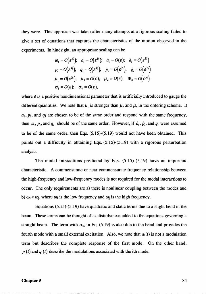
they were. This approach was taken after many attempts at a rigorous scaling failed to

give a set of equations that captures the characteristics of the motion observed in the

experiments. In hindsight, an appropriate scaling can be

rol = o( eM); llt = o( eM); ~ = O(e); ~ = o( e~) Pi = O(eM); qj = q(eM); Pi = O(e~); (t = O(e%)

J.ll = o( eM); J.l3 = O( e); J.l4 = O( e); <1>0 = o( eX)

0'3 = O(e); 0'4 = O(e),

where e is a positive nondimensional parameter that is artificially introduced to gauge the

different quantities. We note that J.ll is stronger than J.l3 and J.l4 in the ordering scheme. If

al, Ph and qi are chosen to be of the same order and respond with the same frequency,

then ~,Pi' and qi should be of the same order. However, if ~,Pi' and qj were assumed

to be of the same order, then Eqs. (5.15)-(5.19) would not have been obtained. This

points out a difficulty in obtaining Eqs. (5.15)-(5.19) with a rigorous perturbation

analysis.

The modal interactions predicted by Eqs. (5.15)-(5.19) have an important

characteristic. A commensurate or near commensurate frequency relationship between

the high-frequency and low-frequency modes is not required for the modal interactions to

occur. The only requirements are a) there is nonlinear coupling between the modes and

b) Oli « Olj, where Oli is the low frequency and Olj is the high frequency.

Equations (5.15)-(5.19) have quadratic and static terms due to a slight bend in the

beam. These terms can be thought of as disturbances added to the equations governing a

straight beam. The term with a40 in Eq. (5.19) is also due to the bend and provides the

fourth mode with a small external excitation. Also, we note that al(t) is not a modulation

term but describes the complete response of the first mode. On the other hand,

pj(t) and qj(t) describe the modulations associated with the ith mode.

Chapter 5 84

5.2 Theoretical Results

Because we were unable to obtain closed-fonn solutions to Eqs. (5.15)-(5.19), we

used numerical methods to investigate the solutions of these equations. The different

branches of fixed points were detennined by using an arc-length continuation method

(Seydel, 1988). An initial point on a branch, where only one solution was expected, was

obtained by numerically integrating Eqs. (5.15)(5.19) for a long time. To find a starting

fixed point on the other branches, we varied the initial guesses until a fixed point on

another branch was found. To detennine the stability of the fixed points, we calculated

the eigenvalues of the Jacobi matrix. To detennine the branches of periodic solutions, we

used a shooting method and a sequential continuation scheme (Seydel, 1988).

In Figs. 5.2a-5.2c, al is the complete response of the first mode and a3 and a4,

where ai = ~ p/ + q/ ' are the amplitudes of the third and fourth modes. Stable fixed

points are shown as solid lines and unstable fixed points are shown as broken and dotted

lines. We note that a fixed point corresponds to a periodic motion of the structure.

Branch <D corresponds to fixed points for which

llt =1: 0, P3 = 0, q3 = 0, P 4 =1: 0, and q4 =1: 0. Both of branches Q) and (3) correspond to

fIXed points for which llt =1: 0, P3 =1: 0, q3 =1: 0, P4 =1: 0, and q4 =1: 0. However, for a given

set of parameter values, the value of a3 on branch Q) is smaller than the corresponding

value of a3 on branch Q). Also, the fixed points on branch (j) are unstable.

In the range 33.00 Hz ;:: fe ;::32.754 Hz, only branch CD was found and the fixed

points are all stable. At the critical value fe=32.754 Hz, a supercritical pitchfork

bifurcation occurs in the response of the third mode; that is, a3' As a result of this

pitchfork bifurcation, branch CD becomes unstable for fe<32.754 Hz, as seen in

Figs 5.2a-5.2c. Branch (2) intersects branch CD at this point. Branch CD regains

stability at fe=31.763 Hz due to a reverse pitchfork bifurcation in the response of the third

ChapterS 85

mode, as seen in Figure 5.2b. Branch (3) intersects branch CD at this point. Branch CD

remains stable in the range 31.763 Hz ~ fe ~ 31.669 Hz. At fe=31.669 Hz, a saddle-node

bifurcation of branch <D occurs. On branch <D we have saddle points for

31.669 Hz>fe>31.682 Hz. At fe=31.683 Hz another saddle-node bifurcation occurs on

branch <D. The shape of branch CD in this region shows similarities to the frequency­

response curve of a Duffing oscillator with a softening-type nonlinearity when subjected

to a primary resonance excitation. Also, the peak in the frequency-response curve is near

the natural frequency of the fourth mode. Based on these two observations, we attribute

this peak and the two saddle-node bifurcations to a primary resonance of the fourth mode.

There are no more bifurcations on branch <D in the frequency range considered.

Branch a> intersects branch <D at the pitchfork bifurcation point fe=32. 7 54 Hz.

For 32.754 Hz ~ fe ~ 32.026 Hz, branch (2) is stable. In this region, when fe is decreased,

a3 increases rapidly with no jump, as seen in Fig. 5.2b. In addition, a} increases while a4

decreases, as seen in Fig. 5.2a and 5.2c. As fe is decreased further, we find that a

supercritical Hopf bifurcation occurs at fe=32.026 Hz. Increasing fe from 31.00 Hz, we

find that a subcritical Hopf bifurcation occurs at fe=31.971 Hz. In the range

31.971 Hz<fe<32.026 Hz, branch (2) is unstable with a complex conjugate pair of

eigenvalues having a positive real part. Branch (2) is stable in the remainder of the

region considered.

In Fig. 5.3, we show the frequency-response curves for all three modes in a small

region of the control parameter that includes the Hopf bifurcation points. The solid lines

in Fig. 5.3 represent stable fixed points, the dashed lines represent unstable fixed points,

and the circles represent the amplitudes of the periodic solutions. During the course of

the sequential continuation, the monodromy matrix associated with the periodic solution

was monitored to determine if additional bifurcations occurred. No bifurcations of the

Chapter 5 86

peliodic solution were found. We note that the amplitudes of the periodic solution

increase smoothly from the right and continue past the second Hopf bifurcation point.

This indicates that the Hopf bifurcation at fe=32.026 Hz is supercritical and that the Hopf

bifurcation at fe=31.971 Hz is subcritical. We have not shown the unstable branch of

periodic solutions in the vicinity of the subcritical Hopf bifurcation point in Fig. 5.3. On

the periodic solution branch, the magnitude of at is much larger than the magnitudes of a3

and a4' We note that a periodic solution of Eqs. (5.15)-(5.19) corresponds to a

quasiperiodic response of the cantilever beam, which was also observed in the

experiments.

Branch 0> intersects branch <D at the pitchfork bifurcation point at fe=31.763 Hz,

as shown in Figs. 5.2a-c. Branch 0> consists entirely of unstable fixed points. This

branch corresponds to the lower unstable branch of a principal parametric resonance of

the third mode. Turning points occur at fe=31.525 Hz and fe=31.649 Hz. In this region

we see that the response curve of the first mode makes a loop. We note that the turning­

points in this region are bifurcations because the number of solutions changes between

one and two locally and an eigenvalue goes to zero. However, these turning-point

bifurcations are not saddle-node bifurcations because the branch is unstable on both sides

of the bifurcation points.

5.3 Comparison of Experimental and Theoretical Results

In Fig. 5.4, we show experimentally obtained frequency-response curves for a

base acceleration of 0.85 grms. Figure 5.4a is for a downward sweep in frequency and

Fig. 5.4b is for an upward sweep in frequency. There is a strong qualitative similarity

between the experimental frequency-response curves and the theoretical frequency­

response curves. We mention that in Fig. 5.4 an approximate conversion from strains to

relative displacements was made by multiplying each mode's contribution to the response

Chapter 5 87

by fi/f3, where fi is the natural frequency of the ith mode. This conversion gives a better

measure of the relative displacements observed during the experiment.

In the experimental downward sweep in frequency, we observed a motion with

the third mode being dominant from 32.74 Hz to 31.00 Hz. Beyond fe=31.00 Hz, the

third mode dropped out of the response. The first mode was present from 32.40 Hz to

31.00 Hz with a large oscillating response between 32.24 Hz and 32.17 Hz. Part of the

first-mode response consisted of a static offset The fourth mode had a small contribution

to the response throughout the experiment. This experimentally observed motion

corresponds to the theoretically obtained branch (2) . The large first-mode response

observed in the experiments corresponds to the region between the Hopf bifurcation

points in the analysis, where large periodic motions of the first mode were predicted (see

Fig. 5.3).

In the experimental downward sweep in frequency, we also observed a response

consisting of the first and fourth modes from fe=32.80 Hz to fe=32.74 Hz. This type of

response was not predicted by the analysis and might be due to a combination resonance.

An analysis similar to that of Dugundji and Mukhopadhyay (1973) may predict this

response.

In the experimental upward sweep in frequency, we observed a motion consisting

of only the fourth mode from fe=31.00 Hz to fe=32.17 Hz. A small increase in the

magnitude of the fourth mode occurred near 31.90 Hz. The first and third modes were

activated at 32.17 Hz and seemed to suppress the response of the fourth mode. The

contribution of the first mode to the response was large from 32.17 Hz to 32.24 Hz and

died out at 32.40 Hz. The third mode continued to contribute to the response until

32.74 Hz. For the remainder of the sweep, there was only a small response due to the

fourth mode. The first part of the upward sweep in frequency corresponds to branch <D in the analysis, which corresponds to llt ':# 0, P3 = 0, q3 = 0, P4 ':# 0" and q4 ':# O. The

ChapterS 88

observed increase in a4 corresponds to the primary resonance of the fourth mode. When

branch <D loses stability, one would expect the response to jump to the available stable

branch (2), which corresponds to at -:F- 0, P3 -:F- 0, q3 -:F- 0, P4 -:F- 0, and q4 -:F- O. On this

branch, a4 is smaller than those on branch CD, as observed in the experiment. The large

aj component corresponds to a principal parametric resonance of the third mode. The

large first-mode response observed in the experiments corresponds to the region between

the Hopf bifurcation points in the analysis, where large periodic solutions of llt were

predicted.

In the range of fe in which the third mode was excited, the analytical results are in

very good qualitative agreement with the experimental results. We show in Fig. 5.5 the

spectrum and Poincare section of an experimentally obtained three-mode response when

the first-mode component was large. We show in Fig. 5.6 the spectra and phase portraits

of numerically obtained responses from the averaged equations in the region between the

Hopf bifurcation points. When we observed the three-mode response in the experiments,

there were sidebands about the ! fe and fe peaks in the spectrum. The sideband spacing 2

fm varied throughout the frequency sweep. The frequency of the first-mode component

of the response was equal to fm. In the excitation frequency range between 32.22 Hz and

32.19 Hz, fm was approximately 0.60 Hz, which is close to the natural frequency of the

first mode. This resulted in a response with a large first-mode component, as shown in

Figs. 5.3a and 5.3b. The spectrum has discrete lines with fm and fe being the discernible

incommensurate frequencies. We show in Fig. 5.5 a Poincare section of this motion; the

points form two small loops. The length of time taken to collect the 512 points for the

Poincare section was about 16.0 seconds. The spectrum and the Poincare section indicate

a two-period quasi-periodic motion in the time span considered. From 600 seconds of

data, the pointwise dimension was found to be about 2.25 for a delay of 0.33 seconds at

n=10. The dimension calculation indicates a chaotically modulated motion when the

Chapter 5 89

response of the beam is examined over a longer length of time. This chaotically

modulated motion might be a result of the noise and other disturbances which may be

present in the experiments but not modeled in the analysis.

Information from the experimental observations guided the theoretical

development. The characteristics of the experimentally obtained three-mode response

suggests that the following mechanisms were involved in the responses. A principal

parametric resonance excited the third mode and a weak primary resonance excited the

fourth mode, as indicated by the frequency of the main response of the third mode being

at .!. fe and the frequency of the main response of the fourth mode being at fe. Also, the 2

shape of the frequency-response curve of the third mode is similar to a frequency-

response curve of a nonlinear softening oscillator subjected to a principal-parametric

resonance excitation. An interaction between the first mode and the modulations of the

third and fourth modes resulted in an exchange of energy between the three modes, as

indicated by the response frequency of the first mode being equal to the modulation

frequency_

The base acceleration used in the experiments was 0.85 g rms. In the numerical

simulations an acceleration of 0.85 g rms was not sufficient for exciting the first mode.

So the level of excitation was increased to 1.55 g rms in order to have the first mode

participate in the response. This discrepancy between the experimental and analytical

results could not be accounted for.

5.4 Concluding Remarks

The interaction between the first mode and modulations associated with the third

and fourth modes is a newly observed mechanism for transferring energy from a high­

frequency excitation to a low-frequency mode. The analytical model developed captures

Chapter 5 90

the essential characteristics of this modal interaction. Also, the analytical model predicts

that a static response of a low-frequency mode can be produced due to interactions with

the dynamic response of high-frequency modes. Guided by this result, further

experiments revealed that this static response of the first mode was present in the

response of the cantilever beam. The form of the developed equations can be used in

future studies to gain insight into the behavior of flexible structures that have many

modes of interest with widely separated frequencies.

Chapter 5 91

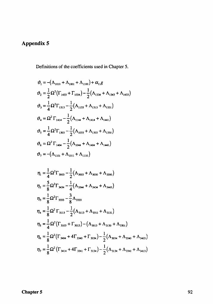
Appendix 5

Definitions of the coefficients used in Chapter 5.

'01 = -( AlOlO + AlOOI + AllOO ) + aug

'02 = .!.02(r1433 + r 1334 ) - .!.(A1334 + Al343 + A1433) 2 2

"'3 = .!.02r1313 - .!.(All33 + Al313 + A1331 ) 4 2

"'4 = 0 2 r 1414 - .!.(AU44 + A1414 + Al44J

2

1 2 1 ( ) "'s = -0 r l303 - - At033 + Al303 + A1330 4 2

'06 = 0 2 r l404 - ..!.(At044 + AI404 + AI440 ) 2

"'7 = -( AllOl + AtOll + All 10 )

Chapter 5 92

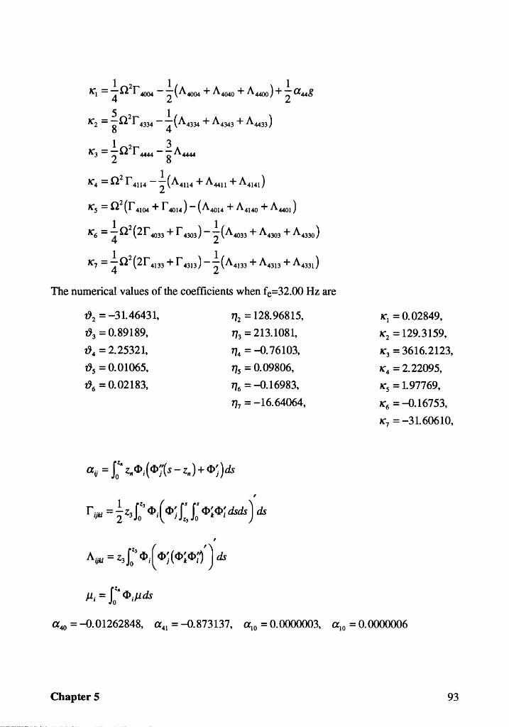
The numerical values of the coefficients when fe=32.00 Hz are

{)2 = -31.46431, 772 = 128.96815, 1('1 = 0.02849,

{)3 = 0.89189, 773 = 213.1081, 1('2 = 129.3159,

{)4 = 2.25321, 774 = -0.76103, 1('3 = 3616.2123,

{)s = 0.01065, 77s = 0.09806, 1('4 = 2.22095,

{)6 = 0.02183, 776 = -0.16983, 1('s = 1.97769,

771 = -16.64064, 1('6 = -0.16753,

1('7 = -31.60610,

,

r iiM = ~ Z3 fo" «I> { «I>j (f: «I>~ «1>; dsds ) tb

,

A ijkl = Z3 f:' «I> { «I>j ( «I>~ «I>j') tb

a 40 = -0.01262848, a41 = -0.873137, a 10 = 0.0000003, a 10 = 0.0000006

ChapterS 93

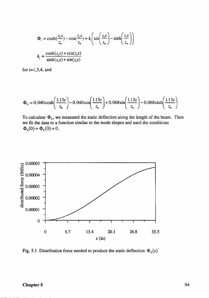
Z·S Z.s (( Z.s) ( Z.s )J CV j =cosh(~)-COS(~)+ki sin ~ -sinh ;n

k. = cosh (ZiS ) + cos( ZiS) , sinh(zjs) + sin(Zis)

for i=1,3,4, and

«1>0 = O. O4OCOShC· ~s ) - O. 040cof· !~S ) + O. 068SinC· !~S ) -O. 068SinhC· !~S ) To calculate CVo' we measured the static deflection along the length of the beam. Then we fit the data to a function similar to the mode shapes and used the conditions

cvo(O) = cvo(O) = O.

=0.00005 S .0 0,0.00004 t)

8 ; 0.00003 £ ::s

=E 0.00002 Cf.I

:.a 0.00001

° o 6.7 13.4 20.1 26.8 33.5

s (in)

Fig. 5.1 Distribution force needed to produce the static deflection CVo{s)'

ChapterS 94

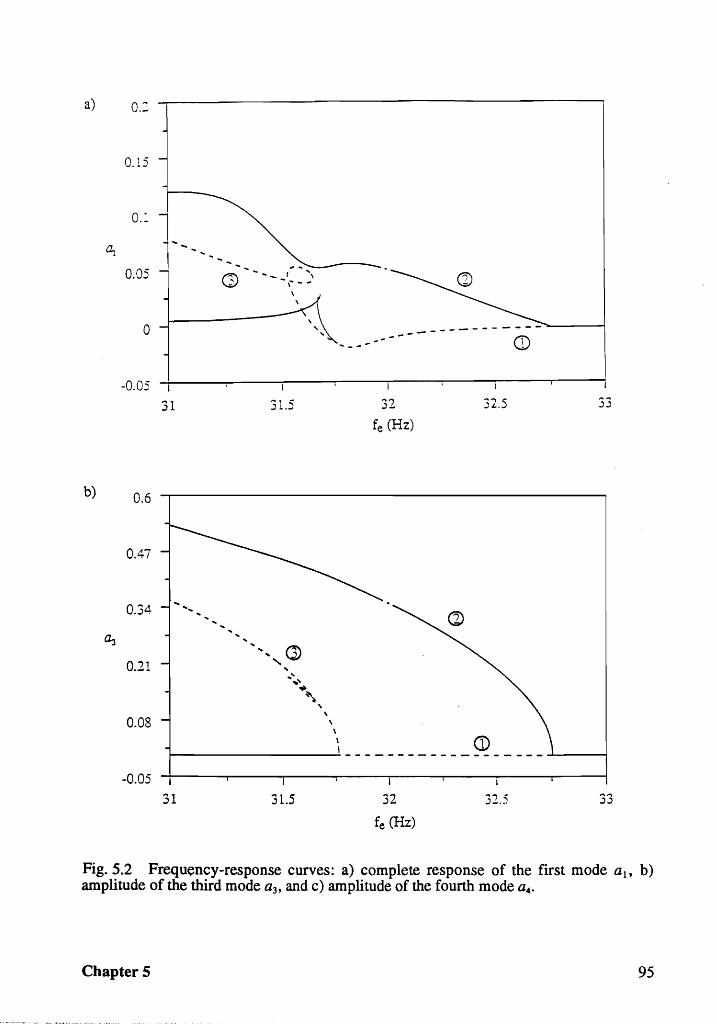
a) 0.2

~

b)

0.15

0.1

0.05 Q)

0 --------~-­_ ..... - ------ CD

-0. 05 -+------:-~-___r--___._--_r_--...-----r_--.--____j

0.6

0.47

0.34

0.21

0.08

31

......

31.5

........ Q)

" ...

, \

\

fe (Hz)

32.5 33

CD ~-------~-------------------~--~

-0.05 -+---......,...--......,...--~--...,..---~--~--r--------1

31 31.5 32 33

fe (Hz)

Fig. 5.2 Frequency-response curves: a) complete response of the first mode al' b) amplitude of the third mode a3' and c) amplitude of the fourth mode a4.

Chapter 5 95

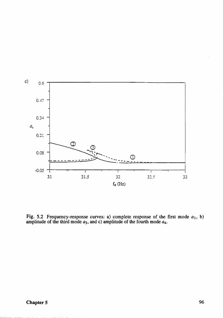
c) 0.6

0..+7

0.34

0.21

0.08 Q)

--------- -------

-0.05 -+-----r----~--~-_.,--___r_-----..,._-____l

31 31.5 32 32.5 33

fe (Hz)

Fig. 5.2 Frequency-response curves: a) complete response of the first mode aI, b) amplitude of the third mode a3, and c) amplitude of the fourth mode a4.

Chapter 5 96

? .,-_._)

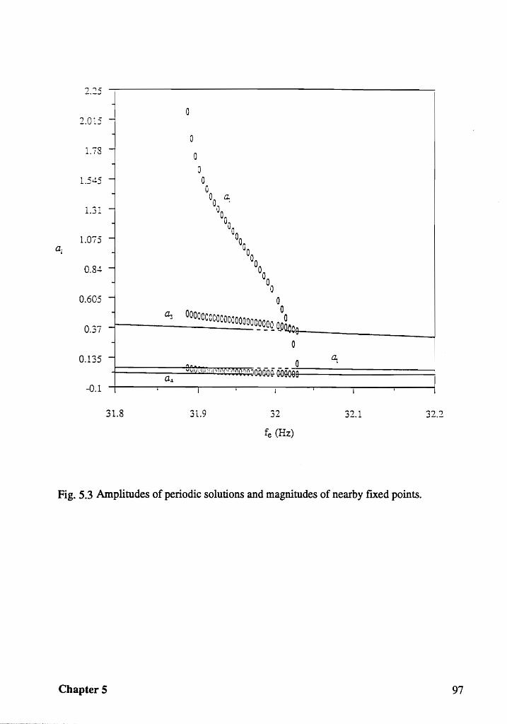
2.015 j -

1.78 --

1.545 -

-1.31 -

-1.075 -

Q,

0.84 --

0.605 -- ~

0.37 --

0.135 -a4

-0.1

31.8

Q

0

0 0 0 0

00 a..

°0 °0

°0 °0

°0 00

00 0

0 0

OOOOCCOCOOOCOOOOOOOOOOO qoO - - - ~Oa. .,

0

1'\", 0 'oJ \ [I ":Id' PI "l(1((\I'\doooo~GoOOGe

I

31.9

I

"'? .J_

fe (Hz)

c;.

I

32.1

Fig. 5.3 Amplitudes of periodic solutions and magnitudes of nearby fIXed points.

Chapter 5

"'? ., .J_._

97

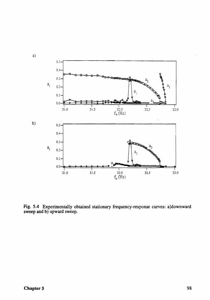
a)

0.5

OA

0.3

a· I 0.:2

0.1

0.0

31.0 31.5 3:::.0 32.5 33.0 fc (Hz)

b) 0.5

0.4

OJ

a· 1 0.2

0.1

0.0

31.0 31.5 32.0 32.5 33.0 fe (Hz)

Fig. 5.4 Experimentally obtained stationary frequency-response curves: a)downward sweep and b) upward sweep.

Chapter 5 98

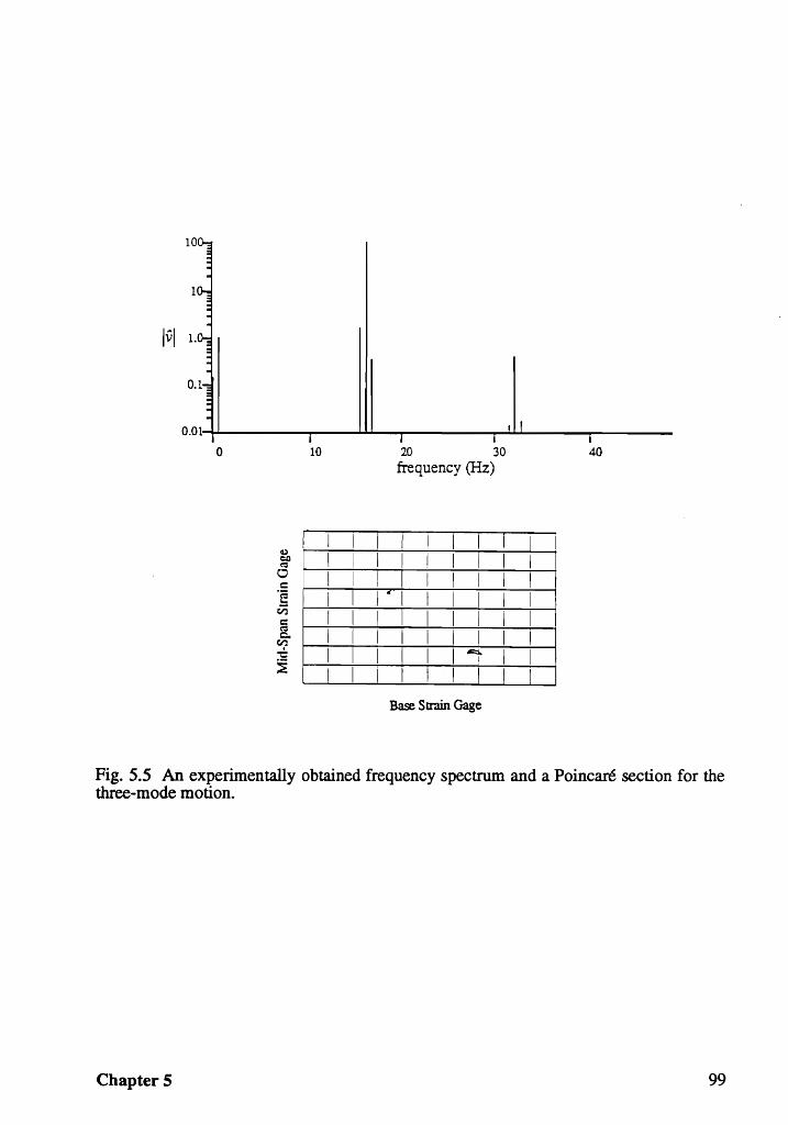
Ivl 1.

0.01~---__ ---U.""--...,.----..,.-l...L.J-_-...,.----

o 10 20 30 40 frequency (Hz)

I I I I I I 1 I I I I I I I , I I I I I I .. I I I I I I I I I I I I I I I I I I I I I I I I I I I I I I .-::::s.. I I I

I , ! I f I T Base Strain Gage

Fig. 5.5 An experimentally obtained frequency spectrum and a Poincare section for the three-mode motion.

Chapter 5 99

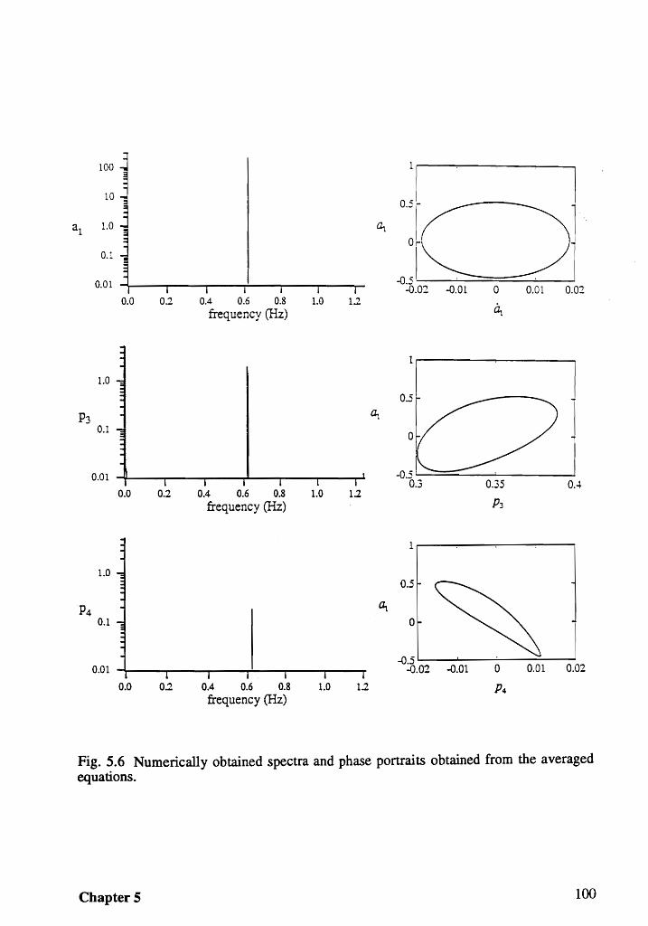
100 j 10

al 1.0 ~ 0.1 J

0.01 J I I I I I

0.0 0.2 0.4 0.6 0.8 1.0 1.2 frequency (Hz)

1.0

P3 0.1

0.01 -y---.,--~----,.J""---_--_-.....,...J.

0.0 0.2 0.4 0.6 0.8 1.0 1.2 frequency (Hz)

1.0

0.01 4---.,---......,.--.,.:...-----..----

0.0 0.2 0.4 0.6 0.8 1.0 1.2 frequency (Hz)

~

:1 1 00°

1 ] ~J~ 1

-0.0: -0.01 0 0.01 0.0:

~

0.5

o

-0.5 L...::=::::::.._...I--___ --1 0.3

0.5

o

0.35

P3

0..+

-O.51---.....I---=---..:::....._......J 0.01 0.02 -0.02 -0.01

Fig. 5.6 Numerically obtained spectra and phase portraits obtained from the averaged equations.

Chapter 5 100

6. Natural Frequencies and Mode Shapes of Laminated Composite Plates: Experiments and FEM

The objective of this chapter is to provide accurate experimental natural

frequencies of several composite plates that can be used to validate future theoretical

developments. In this study, we tried to avoid some of the problems encountered in

similar previous studies, such as, mass loading the structure, using the maximum

response amplitude as a measure of the natural frequency, choice of the material

properties, and unknown boundary conditions.

We determined the natural frequencies and mode shapes of the four composite

plates by using experimental modal-analysis techniques. We tested each plate in a free­

hanging, cantilever, and fIxed-ftxed confIguration for a total of twelve configurations. In

order to eliminate mass loading of the structures, we excited them with an instrumented

impact hammer and measured the response with strain gages. We also calculated the

natural frequencies and mode shapes of the plates by using a finite-element analysis. To

determine the elastic material properties for use in the present finite-element analysis and

future theoretical analyses, we conducted tensile tests on samples made of the same

material and cured with the same cure cycle. Comparing the experimental and theoretical

results, we fInd that the difference between them is less than previously published results.

6.1 Plate Descriptions

In this section, we present the layups, dimensions, and material properties of the

plates. We also describe the methods used to obtain the material properties.

For this study, we manufactured four plates with the following layups:

[-151+ 15/+ 15/-151+ 151-15]s, [-30/+30/+30/-30/+30/-30]8' [9010138, [90/301-301-30130/90]8.

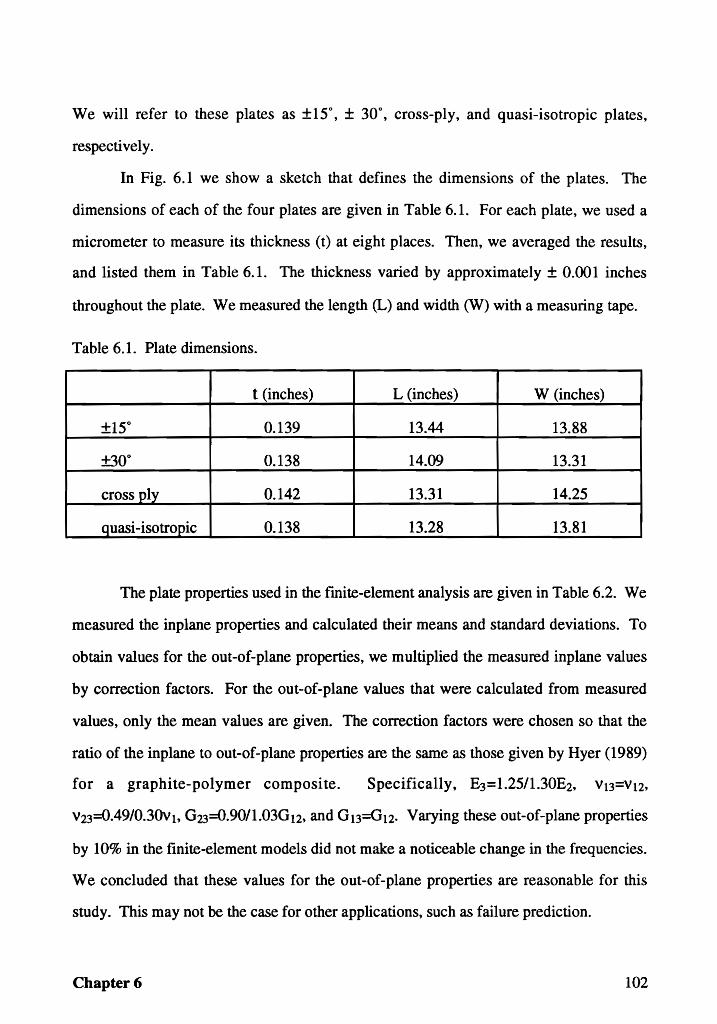
We will refer to these plates as ±15°, ± 30°, cross-ply, and quasi-isotropic plates,

respectivel y.

In Fig. 6.1 we show a sketch that defines the dimensions of the plates. The

dimensions of each of the four plates are given in Table 6.1. For each plate, we used a

micrometer to measure its thickness (t) at eight places. Then, we averaged the results,

and listed them in Table 6.1. The thickness varied by approximately ± OJXH inches

throughout the plate. We measured the length (L) and width (W) with a measuring tape.

Table 6.1. Plate dimensions.

t (inches) L (inches) W (inches)

±15° 0.139 13.44 13.88

±30° 0.138 14.09 13.31

cross ply 0.142 13.31 14.25

quasi-isotropic 0.138 13.28 13.81

The plate properties used in the fmite-element analysis are given in Table 6.2. We

measured the inplane properties and calculated their means and standard deviations. To

obtain values for the out-of-plane properties, we multiplied the measured inplane values

by correction factors. For the out-of-plane values that were calculated from measured

values, only the mean values are given. The correction factors were chosen so that the

ratio of the inplane to out-of-plane properties are the same as those given by Hyer (1989)

for a graphite-polymer composite. Specifically, E3=1.25/1.30E2, V13=V12,

v23=O.49/0.3OVt, 023=0.9011.03012, and 013=012. Varying these out-of-plane properties

by 10% in the finite-element models did not make a noticeable change in the frequencies.

We concluded that these values for the out-of-plane properties are reasonable for this

study. This may not be the case for other applications, such as failure prediction.

Chapter 6 102

To determine the inplane material properties, we made two 12" x 12" plates of the

same material and cured them using the same cure cycle as the plates investigated. One

plate was a uniaxial plate and the other was a symmetric cross-ply plate. A diamond saw

was used to cut out specimens to ensure that the edges were not chipped and delaminated

due to the cutting process. We cut the uniaxial plate into ten test specimens: five had

dimensions 11.0" x 1.0" x 0.092" with the fibers being parallel to the long edges, and five

had dimensions 5.0" x 2.0" x 0.092" with the fibers being perpendicular to the long edges.

We cut the cross-ply plate into five test specimens with dimension 6.0" x 1.0" x 0.1".

The cuts were made at 45 degrees to the plate's edges. This resulted in five ± 45°

specimens. Each of the specimen were instrumented with a biaxial strain gage and pulled

in an Instrom test machine. The load cell had a 10V=10,()(X) lbf calibration for the 0°

specimens and a 10V=2000 lbf calibration for all other specimens. The cross-head rate

was 0.10 in/min for all tests. The axial and transverse strains and the forces were

measured and recorded simultaneously with a PC based data acquisition system. We

later plotted and curve fit the data to obtain the material properties. We used the tensile

tests of the uniaxial specimens to determine the moduli of elasticity Ell and ~2 and

Poisson's ratios Vl2 and V21 similar to the ASTM D 3039-76 test procedure for inplane

tensile properties. We used the tensile tests of the cross-ply specimens to determine the

inplane shear modulus 012 similar to the ASTM D 3518-76 test procedure for inplane

shear properties. Because we were not interested in the strength information, we did not

test the specimens to failure.

To determine the density, we divided the weight by the measured volume. This

was then converted to the appropriate units for mass and volume.

Chapter 6 103

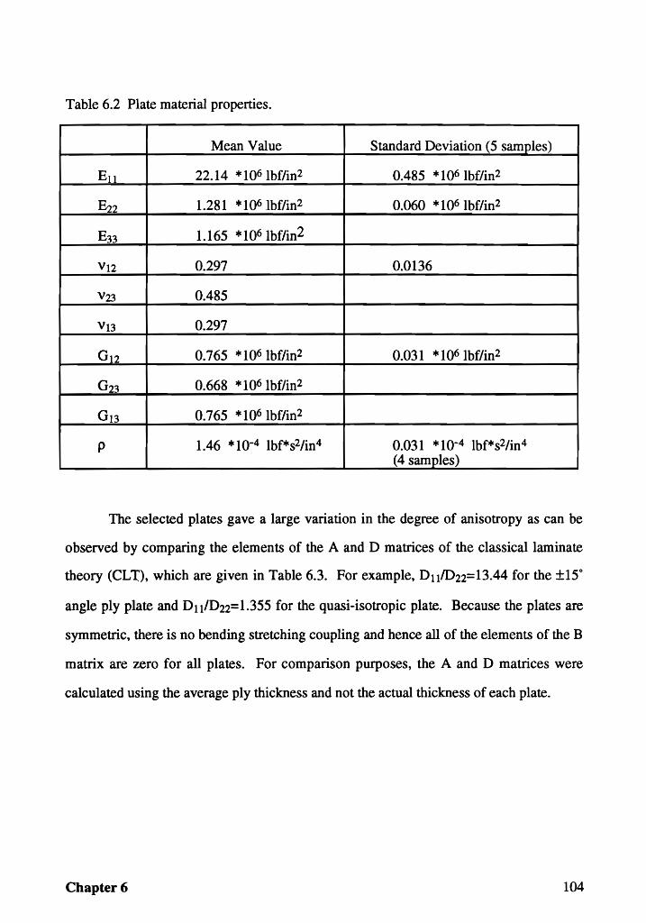
Table 6.2 Plate material properties.

Mean Value Standard Deviation (5 samples)

Ell 22.14 * 106 Ibf/in2 0.485 *106 1bf/in2

~2 1.281 *106 1bf/in2 0.060 * 106 Ibf/in2

E33 1.165 *106 1bf/in2

V12 0.297 0.0136

V23 0.485

V13 0.297

G12 0.765 * 106 Ibf/in2 0.031 *106 1bf/in2

023 0.668 *106 1bf/in2

013 0.765 *106 1bf/in2

p 1.46 *10-4 Ibf*s2/in4 0.031 *10-4 Ibf*s2/in4

(4 samples)

The selected plates gave a large variation in the degree of anisotropy as can be

observed by comparing the elements of the A and D matrices of the classical laminate

theory (CLT), which are given in Table 6.3. For example, D111D22=13.44 for the ±15°

angle ply plate and D11/D22=1.355 for the quasi-isotropic plate. Because the plates are

symmetric, there is no bending stretching coupling and hence all of the elements of the B

matrix are zero for all plates. For comparison purposes, the A and D matrices were

calculated using the average ply thickness and not the actual thickness of each plate.

Chapter 6 104

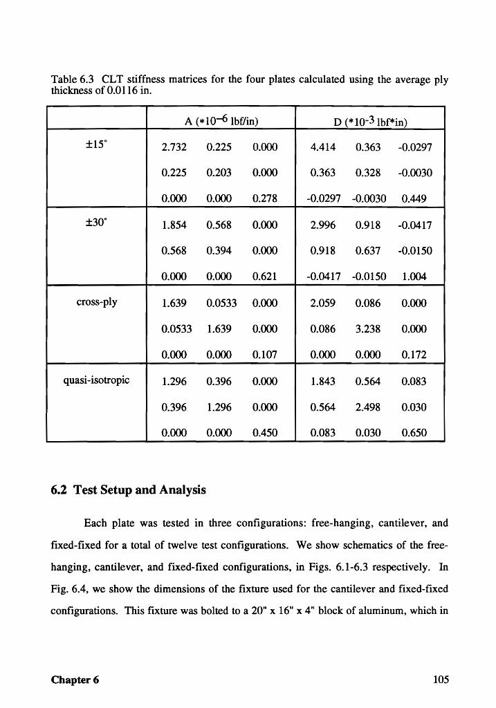
Table 6.3 CLT stiffness matrices for the four plates calculated using the average ply thickness of 0.0116 in.

A (*10-6 lbflin) D (* 10-3 lbf*in)

±15° 2.732 0.225 0.000 4.414 0.363 -0.0297

0.225 0.203 0.000 0.363 0.328 -0.0030

0.000 0.000 0.278 -0.0297 -0.0030 0.449

±30° 1.854 0.568 0.000 2.996 0.918 -0.0417

0.568 0.394 0.000 0.918 0.637 -0.0150

0.000 0.000 0.621 -0.0417 -0.0150 1.004

cross-ply 1.639 0.0533 0.000 2.059 0.086 0.000

0.0533 1.639 0.000 0.086 3.238 0.000

0.000 0.000 0.107 0.000 0.000 0.172

quasi-isotropic 1.296 0.396 0.000 1.843 0.564 0.083

0.396 1.296 0.000 0.564 2.498 0.030

0.000 0.000 0.450 0.083 0.030 0.650

6.2 Test Setup and Analysis

Each plate was tested in three configurations: free-hanging, cantilever, and

fIXed-fixed for a total of twelve test configurations. We show schematics of the free­

hanging, cantilever, and fixed-fixed configurations, in Figs. 6.1-6.3 respectively. In

Fig. 6.4, we show the dimensions of the fixture used for the cantilever and fixed-fIXed

configurations. This fixture was bolted to a 20" x 16" X 4" block of aluminum, which in

Chapter 6 105

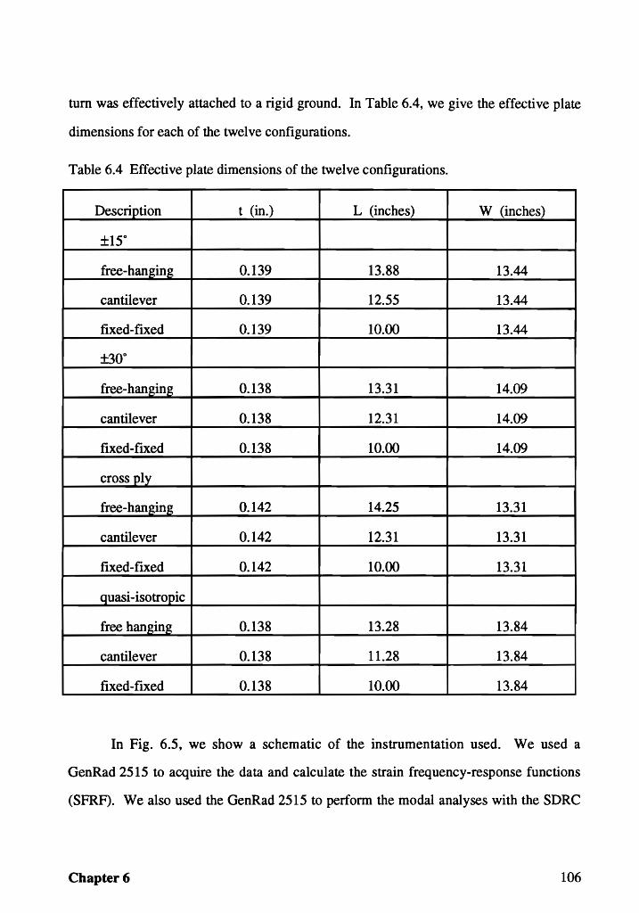
tum was effectively attached to a rigid ground. In Table 6.4, we give the effective plate

dimensions for each of the twelve configurations.

Table 6.4 Effective plate dimensions of the twelve configurations.

Description t (in.) L (inches) W (inches)

±15°

free-hanging 0.139 13.88 13.44

cantilever 0.139 12.55 13.44

fixed-fixed 0.139 10.00 13.44

±30°

free-hanging 0.138 13.31 14.09

cantilever 0.138 12.31 14.09

flXed-fixed 0.138 10.00 14.09

cross ply

free-hanging 0.142 14.25 13.31

cantilever 0.142 12.31 13.31

fixed-fixed 0.142 10.00 13.31

quasi-isotropic

free hanging 0.138 13.28 13.84

cantilever 0.138 11.28 13.84

fixed-fixed 0.138 10.00 13.84

In Fig. 6.5, we show a schematic of the instrumentation used. We used a

GenRad 2515 to acquire the data and calculate the strain frequency-response functions

(SFRF). We also used the GenRad 2515 to perform the modal analyses with the SDRC

Chapter 6 106

Modal-Plus software. To minimize the mass loading of the plates, we chose to excite the

structures with an instrumented impact hammer and measure the responses with strain

gages.

In calculating the SFRFs we used 512 lines of resolution. We chose this

resolution because the analyzer is built in such a way that 512 lines of resolution are the

most convenient for modal analysis. For the free-hanging and cantilever configurations

the tested frequency range was 0-512 Hz. For the fixed-fixed configuration, the tested

frequency range was 0-1024 Hz. To obtain the natural frequencies, mode shapes, and

damping coefficients, we used a polyreference technique available in the SDRC

MODAL-PLUS software (1985). For the free-hanging and cantilever configurations, we

obtained 6 X 6 grids of SFRFs. For the fixed-fixed configurations, we obtained 5 X 5

grids of SFRFs

When using an impact hammer to excite a structure, one must exercise care to

ensure the quality of the obtained data. Corelli and Brown (1984) reviewed some

problems associated with impact testing and means for dealing with them. With these

problems in mind, we took a number of steps to ensure the quality of the obtained data.

We monitored the hammer impulse and a small part of the strain-gage response on an

oscilloscope that was set to trigger by the impulse and freeze the screen. The

oscilloscope had a much higher sampling rate than that used with the signal analyzer.

The use of the oscilloscope enabled us to perform several checks. Based on the peak

value observed on the oscilloscope, we set the full range value of the analyzer to prevent

overloads. Also, we checked for double hits. We often observed double hits and

manually discarded the data if it was not discarded by the signal analyzer. In addition, we

checked the hammer impulse width to ensure that the analyzer acquired at least 6 samples

during the hammer impulse. If the analyzer acquired fewer samples during the impulse,

then either the sample period or the hammer tip was changed for that test. Additionally,

Chapter 6 107

we checked the autospectrum of the impulse to make sure that there was less that 20 db

roll off of the signal in the measurement frequency range. We used an appropriate force

window for the hammer signal from the windows available on the signal analyzer. In

addition, we used an exponential window for both the hammer and strain-gage signals.

When using strain gages to measure the response of a structure, one can obtain the

natural frequencies and modal damping factors with conventional modal-analysis

techniques. In addition, if one gage is used and different SFRFs are obtained by moving

the force (hammer impact location), then mode shapes proportional to the displacement

mode shapes are obtained (Bernasconi and Ewins, 1989). We used thin foil strain gages.

Typically the coherence is good only around the peaks for SFRF. This is sufficient to

extract the modal constants with good precision (Bernasconi and Ewins, 1989).

For the finite-element analysis (FEA) , we used the commercial FEA code

ABAQUS. We used the eight noded quadrilateral element S8R with five integration

points through the thickness (ABAQUS User's Manual, 1989). For all the cases, we used

a uniform 20 X 20 grid of elements. To determine this pattern, we calculated FEA results

with a lOX 10 mesh. We then refined the mesh until there were no significant changes

in the calculated natural frequencies. For the free-hanging configurations, we added soft

springs between the plate and ground to prevent the rigid-body modes from having zero

natural frequencies. It is interesting to note that the free-hanging configurations required

a fmer element mesh than the cantilever or the fixed-fixed configurations for the natural

frequencies to converge.

6.3 Results and Comparisons

In Tables 6.5-6.16, we present the experimental natural frequencies, experimental

damping coefficients, FEA natural frequencies, and the percent difference between the

experimental and FEA natural frequencies. In Figs. 6.6-6.17, we show contour plots of

Chapter 6 108

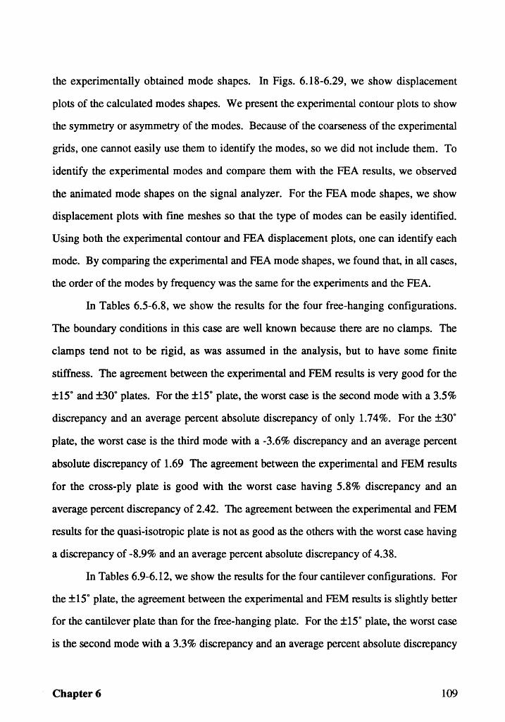
the experimentally obtained mode shapes. In Figs. 6.18-6.29, we show displacement

plots of the calculated modes shapes. We present the experimental contour plots to show

the symmetry or asymmetry of the modes. Because of the coarseness of the experimental

grids, one cannot easily use them to identify the modes, so we did not include them. To

identify the experimental modes and compare them with the FEA results, we observed

the animated mode shapes on the signal analyzer. For the PEA mode shapes, we show

displacement plots with fine meshes so that the type of modes can be easily identified.

Using both the experimental contour and PEA displacement plots, one can identify each

mode. By comparing the experimental and PEA mode shapes, we found that, in all cases,

the order of the modes by frequency was the same for the experiments and the FEA.

In Tables 6.5-6.8, we show the results for the four free-hanging configurations.

The boundary conditions in this case are well known because there are no clamps. The

clamps tend not to be rigid, as was assumed in the analysis, but to have some finite

stiffness. The agreement between the experimental and FEM results is very good for the

±15° and ±30° plates. For the ±15° plate, the worst case is the second mode with a 3.5%

discrepancy and an average percent absolute discrepancy of only 1.74%. For the ±30°

plate, the worst case is the third mode with a -3.6% discrepancy and an average percent

absolute discrepancy of 1.69 The agreement between the experimental and PEM results

for the cross-ply plate is good with the worst case having 5.8% discrepancy and an

average percent discrepancy of 2.42. The agreement between the experimental and FEM

results for the quasi-isotropic plate is not as good as the others with the worst case having

a discrepancy of -8.9% and an average percent absolute discrepancy of 4.38.

In Tables 6.9-6.12, we show the results for the four cantilever configurations. For

the ±15° plate, the agreement between the experimental and FEM results is slightly better

for the cantilever plate than for the free-hanging plate. For the ±15° plate, the worst case

is the second mode with a 3.3% discrepancy and an average percent absolute discrepancy

Chapter 6 109

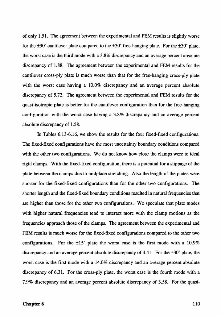
of only 1.51. The agreement between the experimental and FEM results is slightly worse

for the ±30° cantilever plate compared to the ±30° free-hanging plate. For the ±30° plate,

the worst case is the third mode with a 3.8% discrepancy and an average percent absolute

discrepancy of 1.88. The agreement between the experimental and FEM results for the

cantilever cross-ply plate is much worse than that for the free-hanging cross-ply plate

with the worst case having a 10.0% discrepancy and an average percent absolute

discrepancy of 5.72. The agreement between the experimental and FEM results for the

quasi-isotropic plate is better for the cantilever configuration than for the free-hanging

configuration with the worst case having a 3.8% discrepancy and an average percent

absolute discrepancy of 1.58.

In Tables 6.13-6.16, we show the results for the four fixed-fixed configurations.

The fixed-fixed configurations have the most uncertainty boundary conditions compared

with the other two configurations. We do not know how close the clamps were to ideal

rigid clamps. With the fixed-fixed configuration, there is a potential for a slippage of the

plate between the clamps due to midplane stretching. Also the length of the plates were

shorter for the fixed-fixed configurations than for the other two configurations. The

shorter length and the fixed-fixed boundary conditions resulted in natural frequencies that

are higher than those for the other two configurations. We speculate that plate modes

with higher natural frequencies tend to interact more with the clamp motions as the

frequencies approach those of the clamps. The agreement between the experimental and

FEM results is much worse for the fixed-fixed configurations compared to the other two

configurations. For the ±15° plate the worst case is the first mode with a 10.9%

discrepancy and an average percent absolute discrepancy of 4.41. For the ±30° plate, the

worst case is the first mode with a 14.0% discrepancy and an average percent absolute

discrepancy of 6.31. For the cross-ply plate, the worst case is the fourth mode with a

7.9% discrepancy and an average percent absolute discrepancy of 3.58. For the quasi-

Chapter 6 110

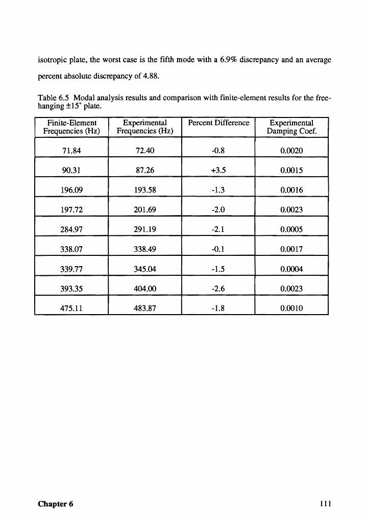
isotropic plate, the worst case is the fifth mode with a 6.9% discrepancy and an average

percent absolute discrepancy of 4.88.

Table 6.5 Modal analysis results and comparison with finite-element results for the free­hanging ±15° plate.

Finite-Element Experimental Percent Difference Experimental Frequencies (Hz) Frequencies (Hz) Damping Coef.

71.84 72.40 -0.8 0.0020

90.31 87.26 +3.5 0.0015

196.09 193.58 -1.3 0.0016

197.72 201.69 -2.0 0.0023

284.97 291.19 -2.1 0.0005

338.07 338.49 -0.1 0.0017

339.77 345.04 -1.5 0.0004

393.35 404.00 -2.6 0.0023

475.11 483.87 -1.8 0.0010

Chapter 6 111

Table 6.6 Modal analysis results and comparison with finite-element results for the free­banging ±30° plate.

Finite-Element Experimental Percent Difference Experimental Frequencies (Hz) Frequencies (Hz) Damping Coef.

84.92 82.77 +2.6 0.0025

130.74 130.97 -0.2 0.0006

209.32 217.23 -3.6 0.0009

260.69 263.56 -1.1 0.0026

280.11 281.50 -0.5 0.0012

353.18 361.49 -2.2 0.0009

474.71 478.97 -0.9 0.0017

Table 6.7 Modal analysis results and comparison with finite-element results for the free­banging cross-ply plate.

Finite-Element Experimental Percent Difference Experimental Frequencies (Hz) Frequencies (Hz) Damping Coef.

58.47 55.28 +5.8 0.0060

203.60 206.98 -1.6 0.0016

233.67 227.60 +2.7 0.0026

235.21 236.00 +0.1 0.0033

261.18 252.27 +3.5 0.0023

391.34 388.19 +0.8 0.0019

Chapter 6 112

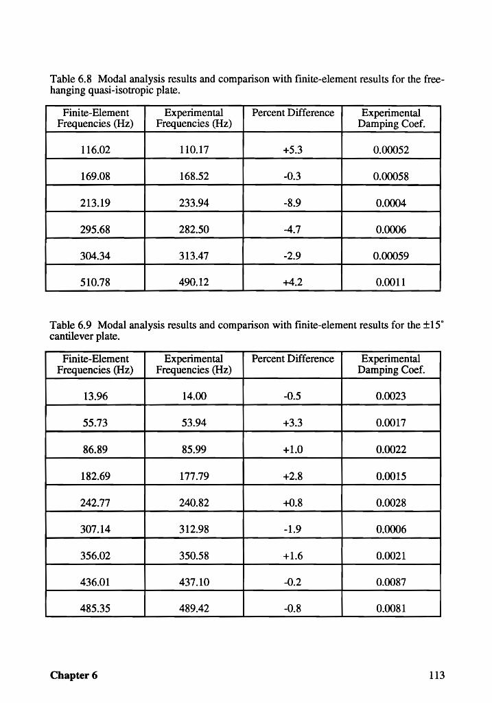
Table 6.8 Modal analysis results and comparison with finite-element results for the free­hanging quasi-isotropic plate.

Finite-Element Experimental Percent Difference Experimental Frequencies (Hz) Frequencies (Hz) Damping Coef.

116.02 110.17 +5.3 0.00052

169.08 168.52 -0.3 0.00058

213.19 233.94 -8.9 0.0004

295.68 282.50 -4.7 0.0006

304.34 313.47 -2.9 0.00059

510.78 490.12 +4.2 0.0011

Table 6.9 Modal analysis results and comparison with finite-element results for the ±15° cantilever plate.

Finite-Element Experimental Percent Difference Experimental Frequencies (Hz) Frequencies (Hz) Damping Coef.

13.96 14.00 -0.5 0.0023

55.73 53.94 +3.3 0.0017

86.89 85.99 +1.0 0.0022

182.69 177.79 +2.8 0.0015

242.77 240.82 +0.8 0.0028

307.14 312.98 -1.9 0.0006

356.02 350.58 +1.6 0.0021

436.01 437.10 -0.2 0.0087

485.35 489.42 -0.8 0.0081

Chapter 6 113

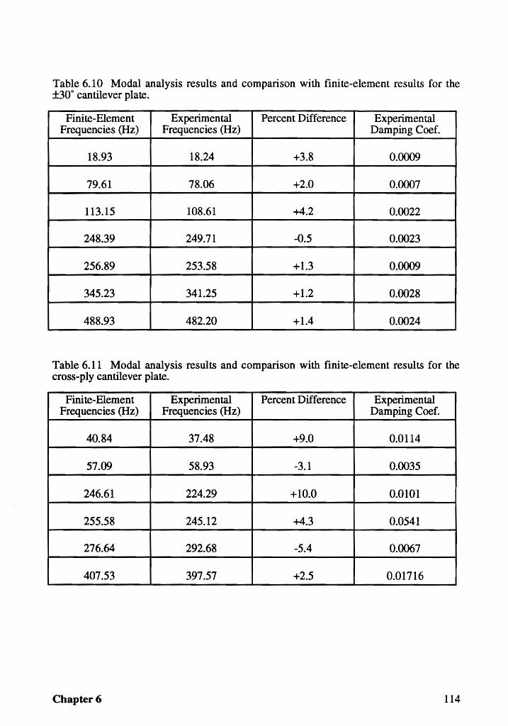
Table 6.10 Modal analysis results and comparison with finite-element results for the ±30° cantilever plate.

Finite-Element Experimental Percent Difference Experimental Frequencies (Hz) Frequencies (Hz) Damping Coef.

18.93 18.24 +3.8 0.0009

79.61 78.06 +2.0 0.0007

113.15 108.61 +4.2 0.0022

248.39 249.71 -0.5 0.0023

256.89 253.58 +1.3 0.0009

345.23 341.25 +1.2 0.0028

488.93 482.20 +1.4 0.0024

Table 6.11 Modal analysis results and comparison with finite-element results for the cross-ply cantilever plate.

Finite-Element Experimental Percent Difference Experimental Frequencies (Hz) Frequencies (Hz) Damping Coef.

40.84 37.48 +9.0 0.0114

57.09 58.93 -3.1 0.0035

246.61 224.29 +10.0 0.0101

255.58 245.12 +4.3 0.0541

276.64 292.68 -5.4 0.0067

407.53 397.57 +2.5 0.01716

Chapter 6 114

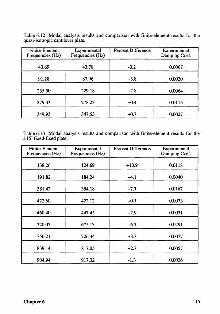
Table 6.12 Modal analysis results and comparison with finite-element results for the quasi-isotropic cantilever plate.

Finite-Element Experimental PercentI>uference Experimental Frequencies (Hz) Frequencies (Hz) I>amping Coef.

43.69 43.78 -0.2 OJXl67

91.28 87.96 +3.8 0.0020

235.50 229.18 +2.8 0.0064

279.33 278.23 +0.4 0.0115

349.93 347.53 +0.7 0.0027

Table 6.13 Modal analysis results and comparison with finite-element results for the ±15° fiXed-fixed plate.

Finite-Element Experimental Percent I>uference Experimental Frequencies (Hz) Frequencies (Hz) I>amping Coef.

138.26 124.69 +10.9 0.0118

191.82 184.24 +4.1 0.0040

381.42 354.18 +7.7 0.0167

422.60 422.12 +0.1 0.0073

460.40 447.45 +2.9 0.0031

720.07 675.13 +6.7 0.0291

750.21 726.44 +3.3 0.0077

839.14 817.05 +2.7 0.0057

904.94 917.32 -1.3 0.0026

Chapter 6 115

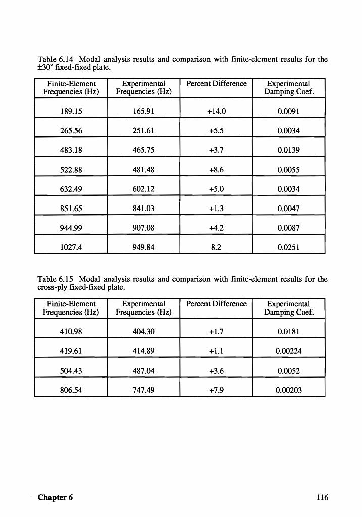
Table 6.14 Modal analysis results and comparison with finite-element results for the ±30° fixed-fixed plate.

Finite-Element Experimental Percent Difference Experimental Frequencies (Hz) Frequencies (Hz) Damping Coef.

189.15 165.91 +14.0 0.0091

265.56 251.61 +5.5 0.0034

483.18 465.75 +3.7 0.0139

522.88 481.48 +8.6 0.0055

632.49 602.12 +5.0 0.0034

851.65 841.03 +1.3 0.0047

944.99 907.08 +4.2 0.0087

1027.4 949.84 8.2 0.0251

Table 6.15 Modal analysis results and comparison with finite-element results for the cross-ply fixed-fIXed plate.

Finite-Element Experimental Percent Difference Experimental Frequencies (Hz) Frequencies (Hz) Damping Coef.

410.98 404.30 +1.7 0.0181

419.61 414.89 +1.1 0.00224

504.43 487.04 +3.6 0.0052

806.54 747.49 +7.9 0.00203

Chapter 6 116

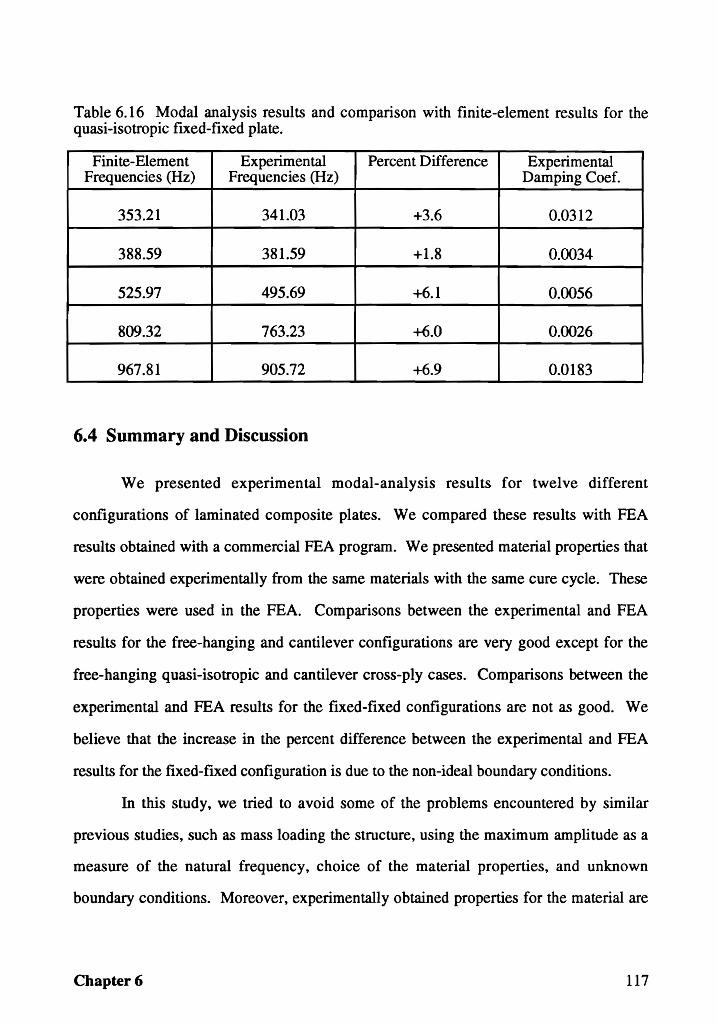
Table 6.16 Modal analysis results and comparison with finite-element results for the quasi-isotropic fIXed-fixed plate.

Finite-Element Experimental Percent Difference Experimental Frequencies (Hz) Frequencies (Hz) Damping Coef.

353.21 341.03 +3.6 0.0312

388.59 381.59 +1.8 0.0034

525.97 495.69 +6.1 0.0056

809.32 763.23 +6.0 0.0026

967.81 905.72 +6.9 0.0183

6.4 Summary and Discussion

We presented experimental modal-analysis results for twelve different

configurations of laminated composite plates. We compared these results with FEA

results obtained with a commercial FEA program. We presented material properties that

were obtained experimentally from the same materials with the same cure cycle. These

properties were used in the FEA. Comparisons between the experimental and FEA

results for the free-hanging and cantilever configurations are very good except for the

free-hanging quasi-isotropic and cantilever cross-ply cases. Comparisons between the

experimental and FEA results for the fixed-fixed configurations are not as good. We

believe that the increase in the percent difference between the experimental and FEA

results for the fixed-fixed configuration is due to the non-ideal boundary conditions.

In this study, we tried to avoid some of the problems encountered by similar

previous studies, such as mass loading the structure, using the maximum amplitude as a

measure of the natural frequency, choice of the material properties, and unknown

boundary conditions. Moreover, experimentally obtained properties for the material are

Chapter 6 117

included. The results of the free-hanging configuration provide accurate experimental

natural frequencies for several composite plates, these results can be used to validate

future theoretical developments. The results of the fixed-fixed configuration can be used

to provide possible explanations for the discrepancies between the measured and

calculated natural frequencies previously reported in the literature.

Chapter 6 118

,

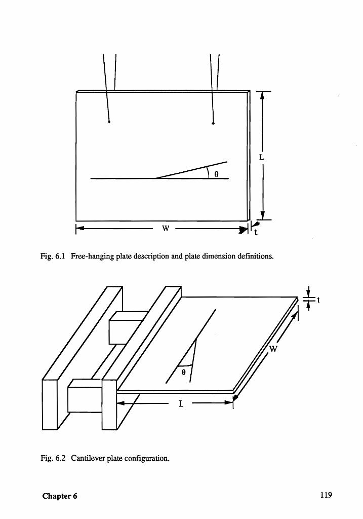
1 4~

L

------r;-

I .... w ----~...,.~

Fig.6.1 Free-hanging plate description and plate dimension definitions.

Fig. 6.2 Cantilever plate configuration.

Chapter 6 119

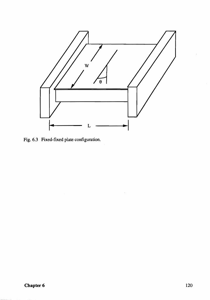
141 L

Fig. 6.3 Fixed-fIXed plate configuration.

Chapter 6 120

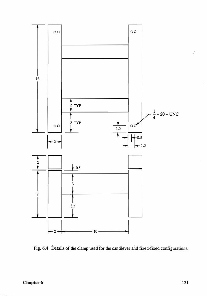
00

16

• 2 TYP r

~

3 TYP 00 ~

t 3

00

/ t 00"

1.0

+ ..... \ H-0.5 ~ . /-.-1.0

D

1 --20-UNC 4

Fig. 6.4 Details of the clamp used for the cantilever and fiXed-fiXed configurations.

Chapter 6 121

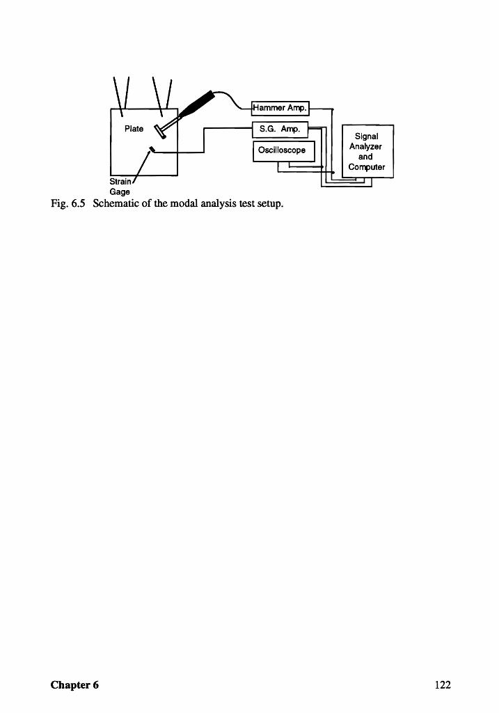
Strain Gage

Fig. 6.5 Schematic of the modal analysis test setup.

Chapter 6

Signal Analyzer

and Computer

122

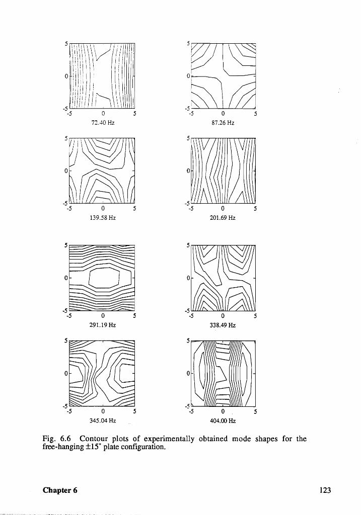
o

o

72.40 Hz

o 139.58 Hz

o 291.19 Hz

o 345.04 Hz

5

5

5

o .... L __

.~----'" ... l_.~ ~ -:J--5 0

o

87.26 Hz

o 201.69 Hz

o 338.49 Hz

o 404.00 Hz

5

5

5

5

Fig. 6.6 Contour plots of experimentally obtained mode shapes for the free-hanging ±15° plate configuration.

Chapter 6 123

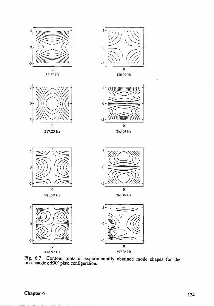
o 82.77 Hz

217.23 Hz

5 ~"-~

o~~ -5~~

o 281.50 Hz

o

5lL~\~ 1 0- ~

J~\@l o

130.97 Hz

:r~1 -5~

o 263.54 Hz

5Z(lQW

-:~oj o

361.49 Hz

5 \ ---=-~

-5 ::;..... -:::::::::::---""" •

o 478.97 Hz 557.06 Hz

Fig. 6.7 Contour plots of experimentally obtained mode shapes for the free-hanging ±30° plate configuration.

Chapter 6 124

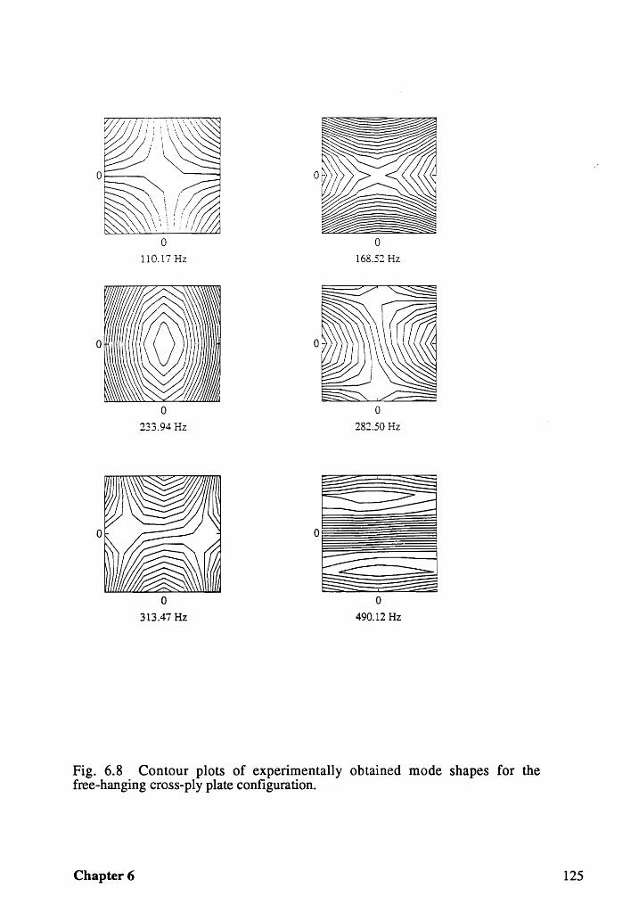
o 110.17 Hz

o 233.94 Hz

o 313.47 Hz

o 168.52 Hz

o 282.50 Hz

o 490.12 Hz

Fig. 6.8 Contour plots of experimentally obtained mode shapes for the free-hanging cross-ply plate configuration.

Chapter 6 125

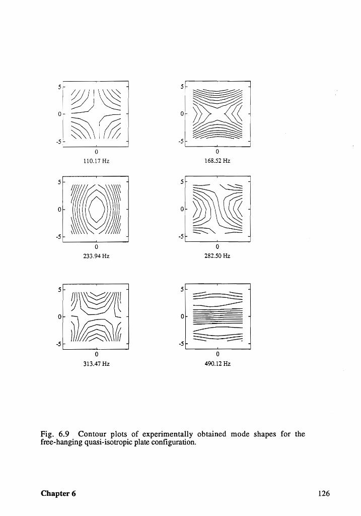
5

0

-5

5

-5

51-

0~ ~@

0

110.17 Hz

o 233.94 Hz

~~~ O"~~0

-51-

0

313.47 Hz

5

~--=~ ~ DrY

-5,..,

5

-5

5

0

-5

0

168.52 Hz

o 282.50 Hz

::::::::::::- -=:::::::: =-------:: --------------::::::::::::-- -::::;:..::::

0

490.12 Hz

Fig. 6.9 Contour plots of experimentally obtained mode shapes for the free-hanging quasi-isotropic plate configuration.

Chapter 6 126

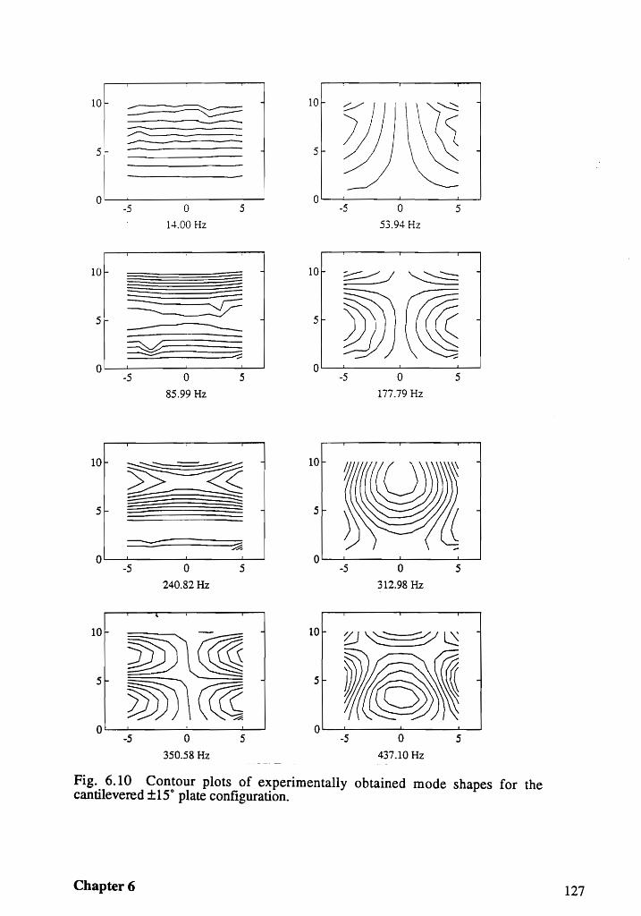
10

5

10

5

0

10

5

0

10

5

,.--.......---­-------

-5

-

a 14.00 Hz

-=.:::. ~ -------~ = ----.;::;---

---·5 0 5

85.99 Hz

-~~ ~ =:::

--- ~

·5 0 5

240.82 Hz

o c.--l __ ......1...-_--'-----'

-5 o 350.58 Hz

5

10 i-

5f-

0

10

5

0

10

5

-5 a 53.94 Hz

5

~...-I ~ -

I~ -5 0 5

177.79 Hz

-5 0 5

312.98 Hz

V~ ~Q

tft~ -5 o

437.10 Hz

5

-

Fig. 6.10 Contour plots of experimentally obtained mode shapes for the cantilevered ±15" plate configuration.

Cbapter6 127

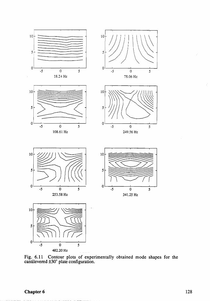
10~ -

==------===:::--------5

---0 I I

-5 0 5

18.24 Hz

o '---"--_--'--__ ..L..--J

-5 o 108.61 Hz

5

-5 0 5

253.58 Hz

482.20 Hz

10

5

0

~) ~ -5

-5

0

78.06 Hz

o 249.56 Hz

5

-5 0 5

341.25 Hz

Fig. 6.11 Contour plots of experimentally obtained mode shapes for the cantilevered ±30° plate configuration.

Chapter 6 128

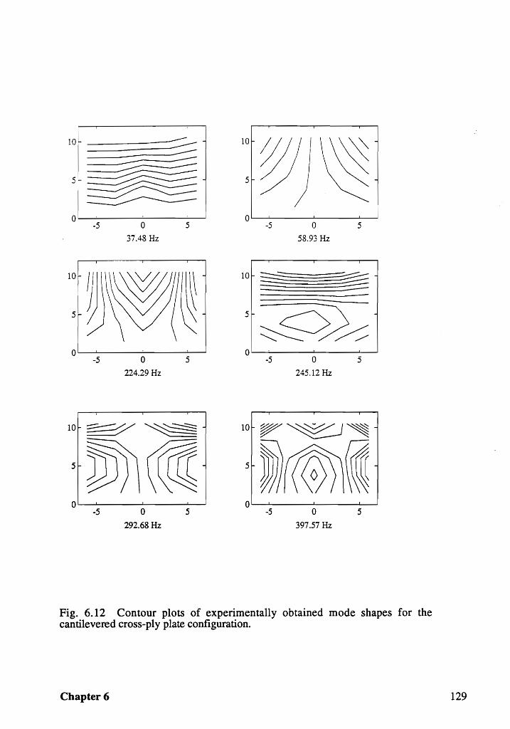
10 ___ ------ ---------------:::::---=--------

=-----= ---5~

--=====---------5

-5

o 37.48 Hz

o 224.29 Hz

5

5

-5

10 ~ -

-5

o 58.93 Hz

o 245.12 Hz

5

5

lO~::::::---~ ~ - lOr-~~~-

5e~~- 5e~~~-01..--..1.------"-----'----'

-5 o 292.68 Hz

5 -5 o 397.57 Hz

5

Fig. 6.12 Contour plots of experimentally obtained mode shapes for the cantilevered cross-ply plate configuration.

Chapter 6 129

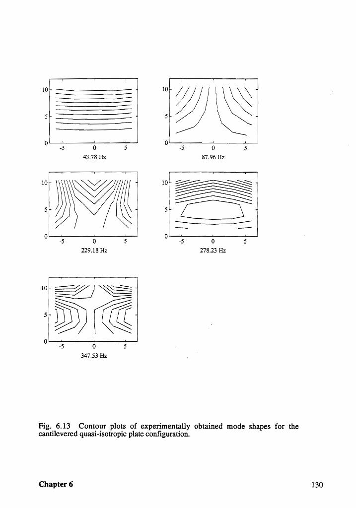
lQl ~_i _____ -

5

-5

10

5

0 -5

-5

o 43.78 Hz

0

229.18 Hz

o 347.53 Hz

5

5

5

5

o~~----~------~

10

5

0

-5 o 87.96 Hz

5

~

~ - ----5 0 5

278.23 Hz

Fig. 6.13 Contour plots of experimentally obtained mode shapes for the cantilevered quasi-isotropic plate configuration.

Chapter 6 130

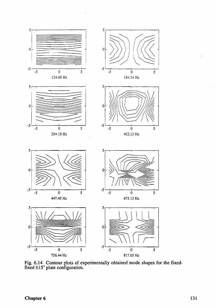
o

-5 '----'-----------""'"'"--' -5 '---'----~-----'--5 0 5 -5 o 5

124.68 Hz 184.24 Hz

-5 '----'-------'---.......... -5 '----'------'------'---' -5 0 5 -5 o 5

354.18 Hz 422.12 Hz

-5 i......-l-_..--L.. __ ..I.---J

-5 0 5

447.45 Hz 675.13 Hz

5,---,.------,---..,.......,

o

-5 ! -5 ~----'----""""" -5 o 5 -5 o 5

726.44 Hz 817.05 Hz

Fig. 6.14 Contour plots of experimentally obtained mode shapes for the fixed­flXed ±15° plate configuration.

Chapter 6 131

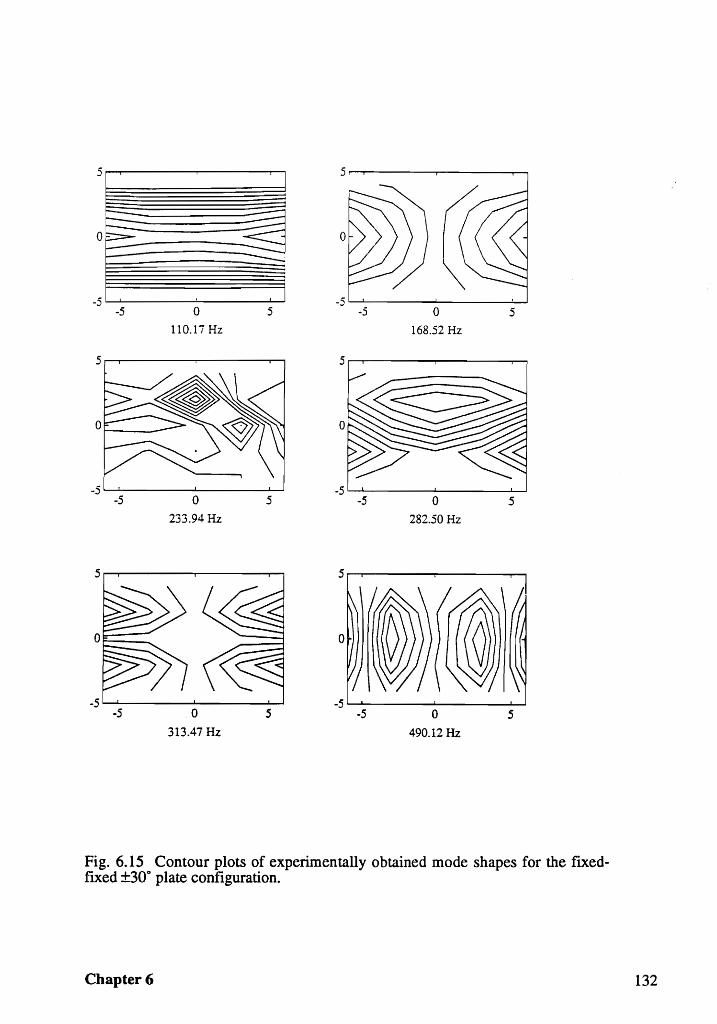
5~------~------~~

o

-5~------~------~~ -5 o

110.17 Hz

5

5~------~------~~

-5 \...-.L. _____ ----I. _____ .--I.--I

-5 o 233.94 Hz

5

5~------~-----~~

OF--___

-5~--------~------~ -5 o

313.47 Hz

5

5~------~------~~

o

-5~------~------~~ -5 o

168.52 Hz 5

5~------~------~~

-5 o 282.50 Hz

5

5~------~--------~

-5~------~------~~ -5 o

490.12 Hz

5

Fig. 6.15 Contour plots of experimentally obtained mode shapes for the flXed­flXed ±30° plate configuration.

Chapter 6 132

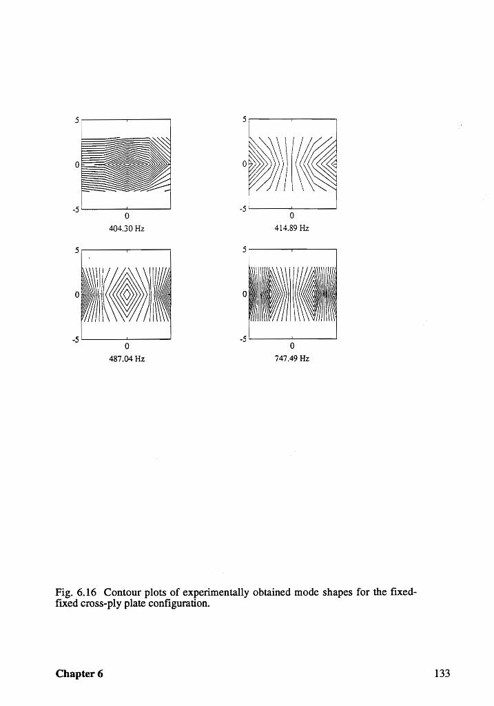
5 51

0 °l)r~ -5 -5

0 0

404.30 Hz 414.89 Hz

5 5

0 I. 0

-5 -5 0 0

487.04 Hz 747.49 Hz

Fig. 6.16 Contour plots of experimentally obtained mode shapes for the flXed­flXed cross-ply plate configuration.

Chapter 6 133

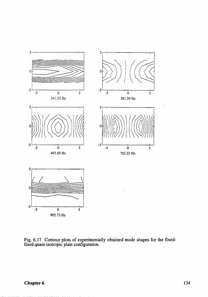
o

-5 !

·5 0 -5 0 5 341.03 Hz 381.59 Hz

-5 0 5 -5 0 5

495.69 Hz 763.23 Hz

~ -~ -r- --

-5 L...-.L......-.--L.....----'---J

-5 0 5

905.72 Hz

Fig. 6.17 Contour plots of experimentally obtained mode shapes for the ftxed­flXed quasi-isotropic plate conftguration.

Chapter 6 134

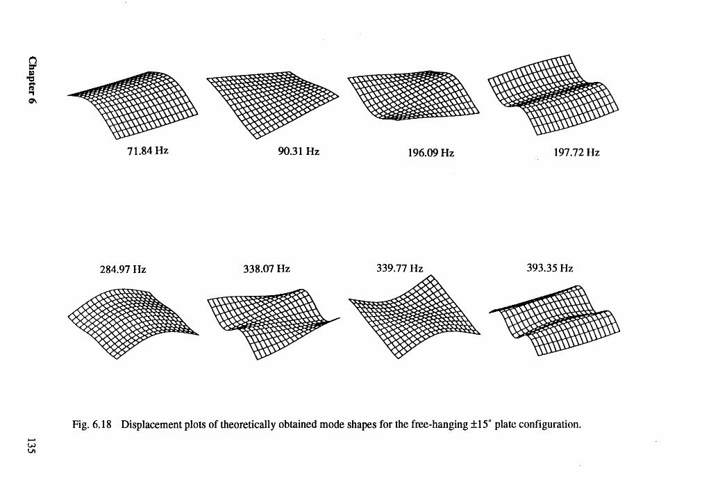
9 fI:I ~

~ c:P\

...... w V\

~ 71.84 Hz 90.31 Hz 196.09 Hz 197.72 Hz

284.97 lIz 338.07 Hz 339.77 Hz 393.35 I-Iz

Fig.6.18 Displacement plots of theoretically obtained mode shapes for the free-hanging ±15° plate configuration .

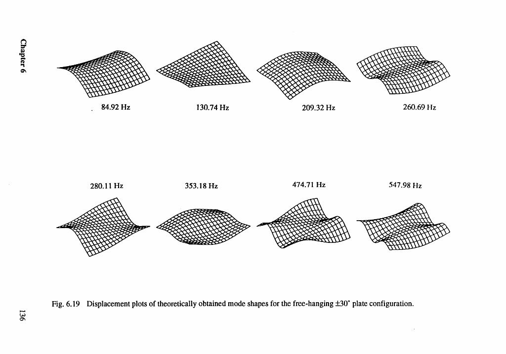
~ ~ f: .., 0\

-W 0'1

84.92 Hz 130.74 Hz 209.32 Hz 260.69 Hz

280.11 Hz 353.18 Hz 474.71 Hz 547.98 Hz

~

Fig.6.19 Displacement plots of theoretically obtained mode shapes for the free-hanging ±30° plate configuration.

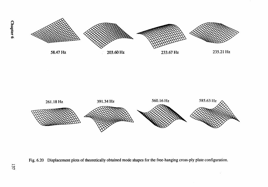
9 ~ ;-.... ~

..... W ....J

58.47 Hz 203.60 Hz 233.67 Hz 235.21 lIz

261.18 Hz 391.34 Hz 560.16 Hz 585.63 Hz

Fig.6.20 Displacement plots of theoretically obtained mode shapes for the free-hanging cross-ply plate configuration .

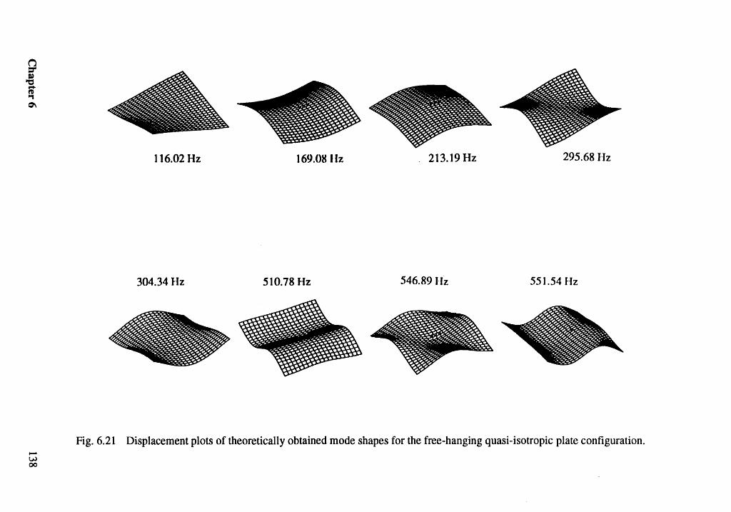
n ::r Q)

"t:S ;-"1

="

..... w 00

116.02 Hz 169.08 lIz 213.19 Hz 295.68 Hz

304.34 Hz 510.78 Hz 546.89 Hz 551.54 Hz

Fig. 6.21 Displacement plots of theoretically obtained mode shapes for the free-hanging quasi-isotropic plate configuration .

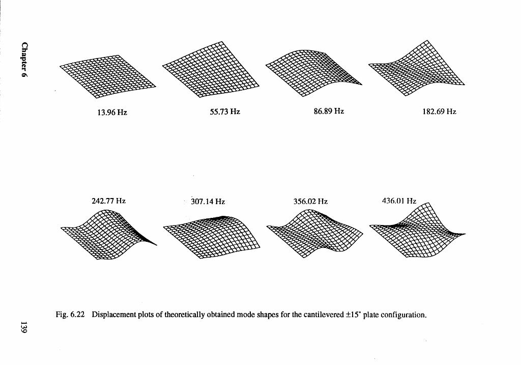
9 ~ ;-.., ~

....... W \0

13.96 Hz 55.73 Hz 86.89 Hz 182.69 Hz

242.77 Hz 307.14 Hz 356.02 Hz

Fig.6.22 Displacement plots of theoretically obtained mode shapes for the cantilevered ±15° plate configuration .

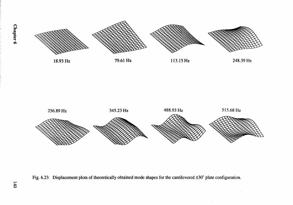
n =" ~

"'CS ;-"1 ~

...... ~

18.93 Hz 79.61 Hz 113.15 Hz 248.39 Hz

256.89 Hz 345.23 Hz 488.93 Hz 515.68 Hz

Fig. 6.23 Displacement plots of theoretically obtained mode shapes for the cantilevered ±30° plate configuration .

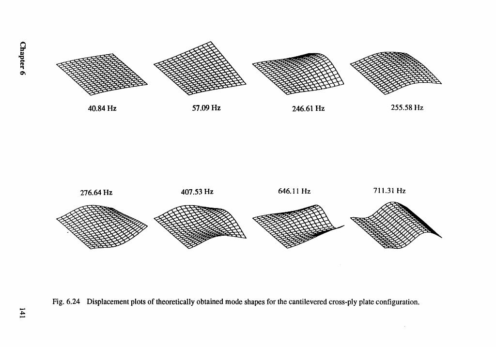
9 ~ ;-.., ~

...... ~ ......

40.84 Hz 57.09 Hz 246.61 Hz 255.58l-Iz

276.64 Hz 407.53 Hz 646.11 Hz 711.31 Hz

Fig. 6.24 Displacement plots of theoretically obtained mode shapes for the cantilevered cross-ply plate configuration .

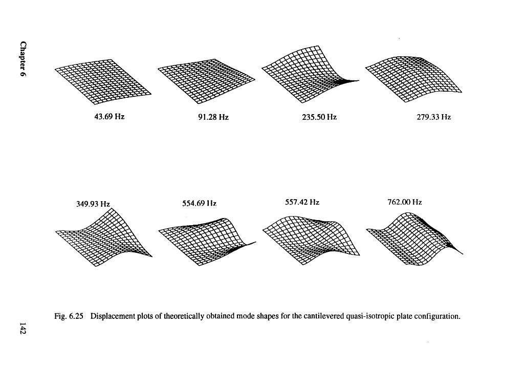
n ::r tQ ~ ;-.., ~

...... ~ tv

43.69 Hz 91.28 Hz 235.50 Hz 279.33 Hz

349.93 Hz 554.69111. 557.42 Hz 762.00 Hz

Fig. 6.25 Displacement plots of theoretically obtained mode shapes for the cantilevered quasi-isotropic plate configuration .

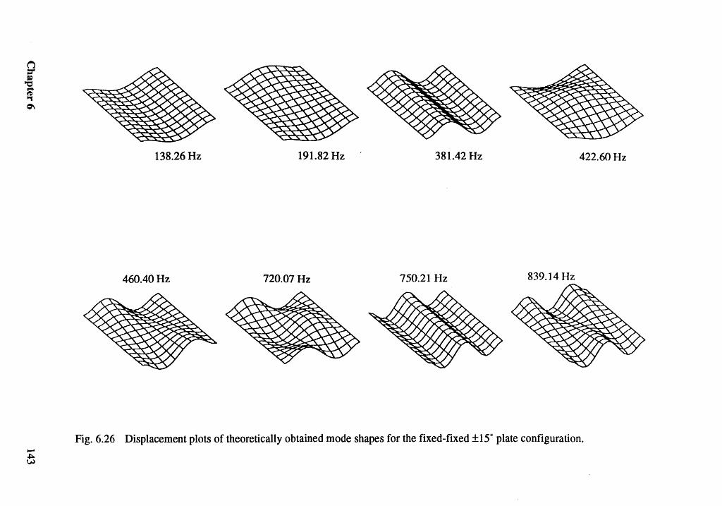
n =­~

"'CS ;i ~

'"

...... ~ w

138.26 Hz 191.82 Hz 381.42 Hz 422.60 Hz

460.40 Hz 720.07 Hz 750.21 Hz 839.14 Hz

Fig.6.26 Displacement plots of theoretically obtained mode shapes for the fixed-fixed ±15° plate configuration .

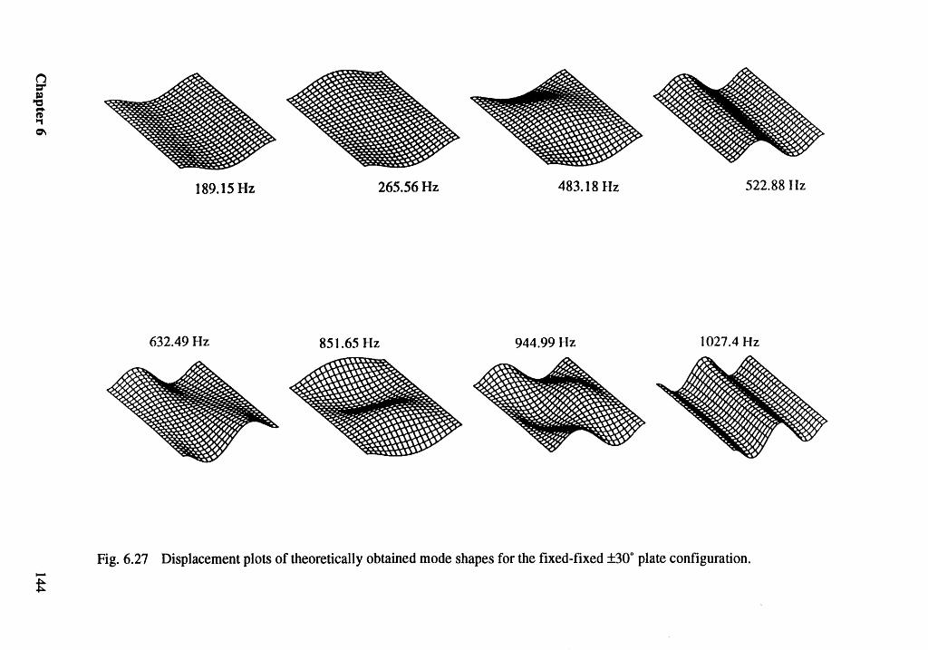
("') =" ~ ;-"'1 ~

...... t

189.15 Hz 265.56 lIz 483.18 Hz 522.88 Hz

632.49 Hz 851.65 Hz 944.99 Hz 1027.4 Hz

Fig. 6.27 Displacement plots of theoretically obtained mode shapes for the fixed-fixed ±30° plate configuration .

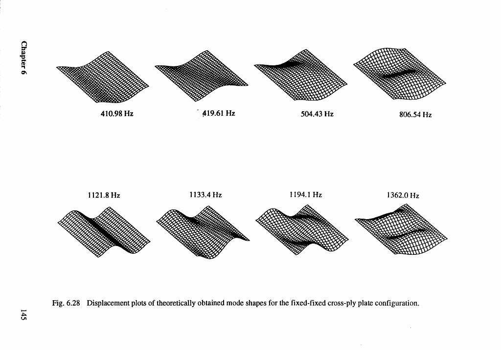
n ::r ~ ~ <:1'\

..... ~

410.98 Hz . ~19.61 Hz 504.43 Hz 806.541-Iz

1121.8 Hz 1133.4 Hz 1194.1 Hz 1362.0 Hz

Fig. 6.28 Displacement plots of theoretically obtained mode shapes for the fixed-fixed cross-ply plate configuration .

(i =" ~

"'CS ;-"'I

'"

""""" ~

353.21 Hz 388.59 Hz 525.97 Hz 809.32 liz

967.81 Hz 1015.6 Hz 1184.2 Hz 1262.5 Hz

Fig. 6.29 Displacement plots of theoretically obtained mode shapes for the fixed-fixed quasi-isotropic plate configuration.

7. Summary and Recommendations

7.1 Summary

Four separate studies were conducted and the results presented. In all of the

studies, we have emphasized the value of combining experimental and theoretical work.

With this combined approach, we verified the importance of the nonlinear curvature in

modeling of cantilever beams. Also, we found that the addition of quadratic damping to

the the model improves the agreement between the experimental and theoretical results

for both frequency-response and force-response curves. Without the quadratic damping

the experimental and theoretical results did not agree even qualitatively for the first mode.

In the two studies involving the multi-mode responses of the slender cantilever

beam, we experimentally discovered a new type of model interaction where the complete

response of a low-frequency mode interacts with the modulations of a high-frequency

mode. Both static and periodic responses of the low-frequency mode were found. We

then developed a model that captures the essential characteristics of this type of motion.

A significant characteristic of this type of modal interaction is that a specific frequency

relationship is not required between the modes involved as is typical of other modal

interactions. The only requirements for this type of modal interaction to occur are that

the frequency of one mode is much higher than the other and there is nonlinear coupling

between the modes. This result may have implications for flexible structures such as the

space station, which have many modes of interest with widely separated frequencies.

We also investigated the natural frequencies and mode shapes of several

laminated composite plates in various configurations. Results from experimental modal

analysis and PEA are presented and compared. Comparisons between experimental and

FEA are much better than what has been previously reported for the free-hanging

configuration where the boundary conditions are well known. Comparisons between the

experimental and FEA are poor for the fixed-fixed configuration indicating that the fixed

boundary conditions significantly deviate from ideal. In this study, we tried to avoid

some of the problems encountered by similar previous studies, such as mass loading the

structure, using the maximum amplitude as a measure of the natural frequency, choice of

the material properties, and unknown boundary conditions. Moreover, experimentally

obtained properties for the material are included. The results of the free-hanging

configuration provide accurate experimental natural frequencies for several composite

plates, these results can be used to validate future theoretical developments. The results

of the fixed-fixed configuration can be used to provide possible explanations for the

discrepancies between the measured and calculated natural frequencies previously

reported in the literature.

7.2 Recommendations

The following topics concerning the nonlinear vibrations of structures are

recommended for future study:

1) Additional experimental investigations need to be conducted to determine if the

transfer of energy from a high-frequency excitation to a low-frequency component in the

response, similar to that reported in Chapters 4 and 5, occurs in other systems.

2) An analysis should be done that includes the out-of-plane motion coupled with the

analysis from Chapter 5 that treats the first mode as a slowly-varying term. This analysis

could be used to explain the experimental results reported in Section 4.3.

3) Additional work in identifying appropriate models for damping is needed. The

identification of damping models must be done experimentally and on a case by case

basis.

148

4) Investigate if modal interactions can occur through coupling that comes only from

nonlinear damping.

5) Experimental investigations of the forced response of laminated composite plates

should be conducted. The results of Chapter 6 can be used to chose forcing frequencies

such that various resonant conditions would be expected to occur.

149

References

ABAQUS User's Manual Version 4.8, 1989, Hibbit, Karlsson & Ssorensen, Inc.

Adams, R. D., and Bacon, D. G. C., 1973, "Measurement of the Flexural Damping

Capacity and Dynamic Young's Modulus of Metals and Reinforced Plastics,"

Journal of Physics D: Applied Physics, Vol. 6, pp. 27-41.

Ashton, J. E., and Anderson, J. D., 1969, "The Natural Modes of Vibration of Boron­

Epoxy Plates," Shock and Vibration Bulletin, No. 39, Part 4, pp. 81-91.

Anand, G. V., 1966, "Nonlinear Resonance in Stretched Strings with Viscous Damping,"

Journal of Acoustical Society of America, Vol. 40, pp. 1517-1528.

Baker, W. E., Woolam, W. E., and Yound, D., 1967, "Air and Internal Damping of Thin

Cantilever Beams," International Journal Mechanical Sciences, Vol. 9, pp. 743-

766.

Banks, H. T., and Inman, D. J., 1991, "On Damping Mechanisms in Beams," Journal of

Applied Mechanics, Vol. 58, pp. 716-723.

Bernasconi, 0., and Ewins, D. J., 1989, "Application of Strain Modal Testing to Real

Structures," Proceedings of the 71h International Modal Analysis Conference, Las

Vegas, NV, Jan. 30-Feb. 2.

Bert, C. W., 1973, "Material Damping: An Introductory Review of Mathematical Models,

Measures and Experimental Techniques," Journal of Sound and Vibration, Vol.

29, pp. 129-153.

Bert, C. W., and Mayberry, B. L., 1969, "Free Vibrations on Unsymmetrically Laminated

Anisotropic Plates," Journal of Composite Materials, Vol. 3. pp. 282-293.

Bert, C. W., 1985, "Research on Dynamic Behavior of Composite and Sandwitch Plates,"

Shock and Vibration Digest, Vol. 17, pp. 3-15.

Bhimaraddi, A., and Stephens, L. K., 1984, "A Higher-Order Theory for Free Vibrations

of Orthotropic, Homogeneous, and Laminated Rectangular Plates," Journal of

Applied Mehcanics, Vol. 51, pp. 195-198.

Bhimaraddi, A., 1987, "Nonlinear Flexural Vibrations of Rectangular Plates SUbjected to

In-Plane Forces Uning a New Shear Deformation Theory," Thin-Walled

Structures, Vol. 5, pp. 309-327.

Brigham, E. 0., 1974, The Fast Fourier Transform, Prentice Hall Inc., New Jersey.

Burton, T. D., and Kolowith, M., 1988, "Nonlinear Resonances and Chaotic Motion in a

Flexible Parametrically Excited Beam,'1 Proceedings of the Second Conference on

Non-linear Vibrations, Stability, and Dynamics of Structures and Mechanisms,

Blacksburg, VA, June 1-3.

Chia, C. Y., 1980, Nonlinear Analysis of Plates, McGraw-Hill, New York.

Clary, R. R., 1972, "Vibration Characteristics of Unidirectional Filamentary Composite

Material Panels," Composite Materials: Testing, Design (Second Conference) ,

ASTM STP 497, pp. 415-438.

Corelli, D., and Brown, D. L., 1984, "Impact Testing Considerations," Proceedings of the

2nd International Modal Analysis Conference, Orlando, FL, Feb. 6-7.

Crandall, S. H., 1970, "The Role of Damping in Vibration Theory," Journal of Sound and

Vibration, Vol. 11, pp. 3-18.

Crawley, E. F., 1979, "The Natural Modes of Graphite/Epoxy Cantilever Plates and

Shells," Journal of Composite Materials, Vol. 13, pp. 195-205.

151

Crespo da Silva, M. R. M., and Glynn, C. C., 1978a, IINonlinear Flexural-Flexural­

Torsional Dyanamics of Inextensional Beams -- I. Equations of Motion," Journal

of Structural Mechanics, Vol. 6, pp. 437-448.

Crespo da Silva, M. R. M., and Glynn, C. C., 1978b, "Nonlinear Flexural-Flexural­

Torsional Dyanamics of Inextensional Beams -- II. Forced Motions," Journal of

Structural Mechanics, Vol. 6, pp. 449-461.

Cusumano, J. P., and Moon, F.C., 1989, "Low Dimensional Behavior in Chaotic

Nonplanar Motions of a Forced Elastic Rod: Experiment and Theory, II Nonlinear

Dynamics in Engineering Systems, IUTAM Symposium, Germany.

Cusumano, J. P., 1990, IILow-Dimensional, Chaotic, Nonplanar Motions of the Elastica:

Experiment and Theory," Ph.D. Dissertation, Cornell University, New York.

Dowell, E. H., Traybar, J., and Hodges, D. H., 1977, "An Experimental-Theoretical

Correlation Study of Nonlinear Bending and Torsion Deformations of a

Cantilever Beam:' Journal of Sound and Vibration, Vol. 50, pp. 533-544.

Dugundji, J., and Mukhopadhyay, V., 1973, "Lateral Bending-Torsional Vibrations of a

Thin Beam Under Parametric Excitation," Journal of Applied Mechanics, Vol.

40, pp. 693-698.

Eringen, A. C., 1952, "On the Nonlinear Vibration of Elastic Bars," Quarterly of Applied

Mathematics, Vol. 9, pp. 361-369.

Evensen, D. A., and Evan-Iwanowski, R. M., 1966, "Effects fo Longitudinal Inertia Upon

the Parametric Response of Elastic Column," Journal of Applied Mechanics, Vol.

33, pp. 141-148.

Ewins, D. J., 1984, Modal Testing: Theory and Practice, Wiley, New York.

Froude, W., 1863, "Remarks on Mr. Scott Russell's Paper on Rolling," Transactions of

Institute of Naval Architects, Vol. 4, pp. 232-275.

152

Gade, S., and Herlufsen, H., 1988, "Windows to FFT Analysis," Sound and Vibration,

Vol. 22, No.3, pp. 14-22.

Haddow, A. G., Barr, A. D. S., and Mook, D. T., 1984, "Theoretical and Experimental

Study of Modal Interaction in a Two-Degree-of-Freedon Structure," Journal of

Sound and Vibration, Vol. 97, pp. 451-473.

Haddow, A. G., and Hasan, S. M., 1988, "Nonlinear Oscillation of a Aexible Cantilever:

Experimental Results," Proceedings of the Second Conference on Non-linear

Vibrations, Stability, and Dynamics of Structures and Mechanisms, Blacksburg,

VA, June 1-3.

Haight, E. C., and King, W. W., 1971, "Stability of Parametrically Excited Vibrations of

and Elastic Rod," Developments in Theoretical and Applied Mechanics, Vol. 5,

pp.677-714.

Harris, F. J., 1978, "On the Use of Windows for Harmonic Analysis with the Discrete

Fourier Transform," Proceeding of the IEEE, Vol. 66, No.1, pp. 51-83.

Heyliger, P. R., and Reddy, J. N., 1988, "A Higher Order Beam Finite Element for

Bending and Vibration Problems," Journal of Sound and Vibration, Vol. 126, pp.

309-326.

Hodges, D. H., and Dowell, E. H., 1974, " Nonlinear Equations of Motion for the Elastic

Bending and Torsion of Twisted Nonuniform Rotor Blades," NASA TN D-7818.

Hodges, D. H., Crespo da Silva, M. R. M., and Peters, D. A., 1988, "Nonlinear Effects in

the Static and Dynamic Behavior of Beams and Rotor Blades," Vertica, Vol. 12,

pp.243-256.

Hyer, M. W., 1989, "Introduction to the Mechanics of Fiber-Reinforced Materials and

Structures," Virginia Polytechnic Institute and State University, College of

Engineering Report VPI-E89-9.

153

Jeffries, C., and Wiesenfeld, K., 1985, "Observation of Noisy Precursors of Dynamical

Instabilities," Physical Review A, Vol. 31, No.2, pp. 1077-1084.

Johnson, J. M., and Bajaj, A. K., 1989, "Amplitued Modulated and Chaotic Dynamics in

Resonant Motion of Strings," Journal of Sound and Vibration, Vol. 128, pp. 87-

107.

Kapania, R. K., and Raciti, S., 1989a, "Recent Advances in Analysis of Laminated Beams

and Plates, Part I: Shear Effects and Buckling," AIAA Journal, Vol. 27, pp. 923-

934.

Kapania, R. K., and Raciti, S., 1989b, "Recent Advances in Analysis of Laminated

Beams and Plates, Part II: Vibration and Wave Propagation," AIAA Journal, Vol.

27, pp. 934-946.

Leissa, A. W., 1981, "Advances in Vibrations, Buckling, and Postbuckling Studies on

Composite Plates," Composite Structures, edited by T. H. Marshall, Applied

Science Publisters, London, pp. 312-334.

Librescu, L., and Reddy, J. N., 1989, itA Few Remarks Concerning Several Refined

Theories of Anisotropic Composite Laminated Plates," International Journal of

Engineering Science, Vol. 27, pp. 515-527.

Mayberry, B. L., and Bert, C. W., 1968 , "Experimental Investigation of Nonlinear

Vibrations of Laminated Anisotropic Panels," The Shock and Vibration Bulletin,

No. 39, Part 3, pp. 191-199.

Miles, J. W., 1962, "Stability of Forces Oscillations of a Spherical Pendulum," Quarterly

of Applied Mathematics, Vol. 20, pp. 21-32.

Miles, J. W., 1965, "Stability of Forced Oscillations of a Vibrating String, Journal of

Acoustical Society of America, Vol. 38, pp. 855-861.

154

Moon, F. C., and Holmes, P. J., 1979, "A Magneto-Elastic Strange Attractor," Journal of

Sound and Vibration, Vol. 65, pp. 275-296.

Moon, F. C., 1980, "Experiments on Chaotic Motions of a Forced Nonlinear Oscillator:

Strange Attractors,'t Journal of Applied Mechanics, Vol. 47, pp. 638-644.

Moon, F. C., and Holmes, W. T., 1985, "Double Poincare Sections of a Quasi­

Periodically Forced Chaotic Attractor," Physics Letters A, Vol. 111, No.4, pp.

157-160.

Moon, F. C., and Shaw, S. W., 1983, "Chaotic Vibrations of a Beam with Nonlinear

Boundary Conditions,tI International Journal of Non-Linear Mechanics, Vol. 18,

pp.465-477.

Narasimha, R., 1968, ttNonlinear Vibration of an Elastic String," Journal of Sound and

Vibration, Vol. 8, pp. 134-136.

Nayfeh, A. H., Mook, D. T., and Marshall, L. R., 1973, tlNonlinear Coupling of Pitch and

Roll Modes in Ship Motions," Journal ofHydronautics, Vol. 7, pp. 145-152.

Nayfeh, A. H., and Mook, D. T., 1979, Nonlinear Oscillations, Wiley, New York.

Nayfeh, A. H., 1981, Introduction to Perturbation Techniques, Wiley, New York.

Nayfeh, A. H., 1983, ttCombination Resonances in the Non-Linear Response of Bowed

Structures to a Harmonic Excitation," Journal of Sound and Vibration, Vol. 90,

pp.457-470.

Nayfeh, A. H., 1984, "On the Low-Frequency Drumming of Bowed Structures," Journal

of Sound and Vibration, Vol. 94, pp. 551-562.

Nayfeh, A. H., and Zavodney, L. D., 1988, "Experimental Observations of Amplitude­

and Phase-Modulated Responses of Two Internally Coupled Oscillators to a

Harmonic Excitation," Journal of Applied Mechanics, Vol. 55, pp. 706-711.

155

Nayfeh, A. H., Balachandran, B., Colbert, M. A., and Nayfeh, M. A., 1989, "An

Experimental Investigation of Complicated Responses of a Two-Degree-of

Freedom Structure," Journal of Applied Mechanics, Vol. 56, pp. 960-967.

Nayfeh, A. H., and Balachandran, B., 1993, Applied Nonlinear Dynamics, Wiley, New

York.

Nayfeh, S. A., Nayfeh, A. H., and Mook, D. T., 1992, "Modal Interactions in a

Parametrically and Externally Excited String," Proceedings of the Fourth

Conference on Nonlinear Vibrations, Stability, and Dynamics of Structures and

Mechanisms, Blacksburg, VA, June 7-11.

Nayfeh, T. A., Nayfeh, A. H., and Mook, D. T., 1990, "A Theoretical-Experimental

Investigation of a Three-Degree-of-Freedom Structure," AIAA Paper No. 90-1081,

AIAA 31st Structure, Structural Dyanmics and Materials Conference, Long

Beach, CA.

Nelson, F. C., and Greif, R., 1970, tlDamping", Shock and Vibration Computer

Programs: Reviews and Summaries, Vol. 23, pp. 237-245.

Pai, P. F., and Nayfeh, A. H., 1991, "A Nonlinear Composite Plate Theory,tI Nonlinear

Dynamics, Vol. 2, pp. 445-477.

Pai, P. F., and Nayfeh, A. H., 1992, "A Nonlinear Composite Beam Theory," Nonlinear

Dynamics, Vol. 3, pp. 273-303.

Rades, M., 1983, "Identification of the Dyanmic Characteristics of a Simple System with

Qaudratic Damping," Rev. Roum. Sci. Techn.-Mec. Appl., Vol. 28, No.4, pp. 439-

446.

Reddy, J. N., 1983, tlA Review of the Literature on Finite-Element Modeling of

Laminated Composite Plates and Shells," Shock and Vibration Digest, Vol. 15,

pp.3-8.

156

Reddy, J. N., 1984a, "A Simple Higher-Order Theory for Laminated Composite Plates,"

Journal of Applied Mechanics, Vol. 51, pp. 745-762.

Reddy, J. N., 1984b, "A Refined Nonlinear Theory of Plates with Transverse Shear

Deformation," International Journal of Solids and Structrues, Vol. 20, pp. 881-

896.

Reddy, J. N., 1985, "A Review of the Literature on Finite-Element Modeling of

Laminated Composite Plates and Shells," Shock and Vibration Digest, VoL 17,

pp.3-8.

Reference Manual for Modal-Plus, 1985, Structural Dynamics Research Corporation.

Reissner, E., 1948, "Finite Deflections of Sandwitch Plates:' Journal of the Aeronautical

Sciences, Vol. 15, pp. 435-440.

Reissner, E., 1953, "On Variational Theory for Finite Elastic Deformation," Journal of

Mathenultical Physics, Vol. 32, pp. 129-135.

Rice, H. J., and Fitzpatrick, J. A., 1991, "The Measurement of Nonlinear Damping in

Single-Degree-of-Freedom Systems," Journal of Vibration and Acoustics, Vol.

113, pp. 132-140.

Sato, K., Saito, H., and Otomi, K., 1978, "The Parametric Response of a Horizonatal

Beam Carrying a Concentrated Mass Under Gravity," Journal of Applied

Mechanics, Vol. 45, pp. 643-648.

Schmidt, R., 1977, itA Refined Nonlinear Theory of Plates with Transverse Shear

Deformations," Journal of Industrial Mathematics Society, Vol. 27, Part 1, pp. 23-

28.

157

Singh, G., Rao, G. V., and Iyengar, N. G. R., 1991, "Some Observations on the Large

Deflecton Bending of Rectangular Antisymmetric Cross-Ply Plates," Composite

Structures, Vol. 18, pp. 77-91.

Thomson, W. T., 1981, Theory of Vibration with Applications, Prentice-Hall, Inc., New

Jersey.

Timoshenko, S. P., 1921, "On the Correction for Shear of the Differential Equation for

Tranverse Vibrations of Prismatic Bars," Philosophical Magazine, Vol. 41, pp.

744-746.

Timoshenko, S. P., 1922, "On the Transverse Vibrations of Bars of Uniform Cross

Sections," Philosophical Magazine, Vol. 43, pp. 125-131.

Whitney, J. M., and Leissa, A. W., 1969, "Analysis of Heterogeneous Anisotropic

Plates," Journal of Applied Mechanics, Vol. 36, pp. 261-266.

Wiesenfeld, K., 1985, "Noisy Precursors of Nonlinear Instabilities," Journal of Statistical

Physics, Vol. 38, Nos. 516, pp. 1071-1097.

Yamaki, M., and Chiba, M., 1983, "Nonlinear Vibrations of a Clamped Rectagular Plate

with Initial Deflection and Initial Edge Displacement--Part I: Theory, tI Thin­

Walled Structures, Vol. 1, pp. 3-29.

Yamaki, M., and Chiba, M., 1983, "Nonlinear Vibrations of a Clamped Rectagular Plate

with Initial Deflection and Initial Edge Displacement--Part II: Experiment," Thin­

Walled Structures, Vol. 1, pp. 101-119.

158

Vita

Tony Joseph Anderson was born on August 26, 1960 in Salt Lake City, Utah to

Douglas and Janet Anderson. After graduating from high school in 1978, he attended

Utah State University on an athletic scholarship in track and cross-country. He received a

B.S. degree in Mechanical Engineering from Utah State University in 1983. Because

jobs were scarce, he attended Arizona State University, where he worked towards a M.S.

in Mechanical Engineering. In 1984 he married Jonna Olson Anderson who he met while

at Utah State.

In the fall of 1984, Tony joined Space Data Corporation in Tempe, Arizona.

While at Space Data, he worked as a Mechanical Engineer on a wide assortments of tasks

related to building and launching rockets. While working at Space Data he continued to

work on a masters degree that he received from Arizona State University in 1987. In

1989, Tony, Jonna and family left Arizona for Virginia so Tony could work towards a

Ph.D. in the Department of Engineering Science and Mechanics at Virginia Polytechnic

Institute and State University. In April 1993, he received a Ph.D. degree in Engineering

Mechanics.

Tony and Jonna have three children, Danielle 8, Tana 6, and Kyle 5.

159