applying fixed box model to predict the concentrations...

http://www.iaeme.com/IJCIET/index.asp 159 [email protected]

International Journal of Civil Engineering and Technology (IJCIET)

Volume 7, Issue 2, March-April 2016, pp. 159–170, Article ID: IJCIET_07_02_013

Available online at

http://www.iaeme.com/IJCIET/issues.asp?JType=IJCIET&VType=7&IType=2

Journal Impact Factor (2016): 9.7820 (Calculated by GISI) www.jifactor.com

ISSN Print: 0976-6308 and ISSN Online: 0976-6316

© IAEME Publication

APPLYING FIXED BOX MODEL TO

PREDICT THE CONCENTRATIONS OF

(PM10) IN A PART OF AL-KUT CITY, WASIT

PROVINCE (IRAQ)

Ali Abdul Khaliq Kamal

Building and Construction Engineering, Environmental Department,

Master Student at University of Technology Baghdad, Iraq

Prof. Dr. Abdul Razzak T. Ziboon


University of Technology Baghdad, Iraq

Dr. Zainab Bahaa Mohammed


University of Technology Baghdad, Iraq

ABSTRACT

This paper offers the applying of Fixed Box Model to predict the

concentration of particulate matter of 10 micrometers (PM10) one of the air

pollutants that most commonly affects people's health. The input parameters

(area source capacity of PM10, wind speed, mixing height, size of area source)

were estimated based on the area source emission inventory results including:

road source, mobile source, construction source, industry source and

household domestic source in a part of AL-Kut District. This emission

inventory project was carried out during five months period from November

2015 to March 2016.

The aim of this study was to present that fixed box model east-to-use for

evaluating the presence of air pollution over AL-Kut city.

The calculated results from the model were such closer to the results

founded by using portable equipment for the study area.

Cite this Article: Ali Abdul Khaliq Kamal, Prof. Dr. Abdul Razzak T. Ziboon

and Dr. Zainab Bahaa Mohammed, Applying Fixed Box Model To Predict

The Concentrations of (Pm10) In A Part of Al-Kut City, Wasit Province

(Iraq), International Journal of Civil Engineering and Technology, 7(2), 2016,

pp. 159–170.

http://www.iaeme.com/IJCIET/issues.asp?JType=IJCIET&VType=7&IType=2

http://www.iaeme.com/IJCIET/issues.asp?JType=IJCIET&VType=7&IType

Ali Abdul Khaliq Kamal, Prof. Dr. Abdul Razzak T. Ziboon and Dr. Zainab Bahaa

Mohammed


1. INTRODUCTION The use of comprehensive air quality models started in the late 1970s [1] and since

then, their development has increased rapidly, together with the fast increase in

computational resources. Today, the scientific community develops more, more

complex, and computationally expensive numerical models, and their results made

available to the environmental authorities dealing with the development of air quality

plans and regulations. Models may serve as very useful tools for indirect estimation of

human exposure. As already stated, it is not possible to perform monitoring in all the

various environments that the population meets. Lifetime exposure cannot be measure

directly, and for this kind of study, modeling is the only option. Furthermore, data

from air quality models can supplement the monitoring data for performing mapping

of pollution concentrations in the various microenvironments in which monitoring is

not performed. For model tools to be useful in exposure studies, they need to be well

tested and they need to describe the dominating physical and chemical processes in

the atmosphere at the given location [2]. Present-day numerical air quality models

seen as important tools for the assessment and forecast of air pollutant concentrations

and depositions, contributing to the development of effective strategies for the control

and reduction of air pollutant emissions [3].

The forecasting of air quality is one of the topics of air quality research today due

to urban air pollution and specifically pollution episodes i.e. high pollutant

concentrations causing adverse health effects and even premature deaths among

sensitive groups such as asthmatics and elderly people [4]. The impact of air pollution

on urban environments has become an important research issue [5], leading to

numerous modeling studies related to the influence of buildings and other urban

structures on pollutant accumulation and dissipation patterns. A wide variety of

operational warning systems based on empirical, causal, statistical and hybrid models

have been developed in order to start preventive action before and during episodes

[6].

Modeling approaches to predict pollutant concentrations based on emission

sources and environmental conditions are commonly used tools in air pollution and

climate studies [7]. The forecasting of air quality is one of the topics of air quality

research today due to urban air pollution and specifically pollution episodes i.e. high

pollutant concentrations causing adverse health effects and even premature deaths

among sensitive groups such as asthmatics and elderly people [4].

Air quality models predict air quality in terms of the concentration of specified

pollutants in the air at a certain place. All air quality models need two kinds of input:

1. information about the input pollutants found in the air from one or more sources;

and 2. information about factors that influence the dispersion of pollutants through the

air such as wind speed and direction, presence of high buildings, presence of hills

around the city, etc. The models use all of this information to mathematically

calculate and simulate how pollutants will spread, giving estimates of specific

concentrations at specific places. Some models are very simple, while others are more

complex, including such data as ground level elevation and chemical reactions taking

place in the atmosphere that change the concentration of pollutants in the air. There

are many approaches to modeling, each approach having its strengths and

weaknesses.

Using different models or, even better, combining modeling with other assessment

techniques, significantly improves the reliability of a model [8]. Fixed-box model is a

low cost air pollution modeling method for roughly and quickly estimate the pollutant

Applying Fixed Box Model To Predict The Concentrations of (Pm10) In A Part of Al-Kut

City, Wasit Province (Iraq)


concentration in urban atmosphere [9]. Air quality models now used extensively for

the purpose of air quality management. Whilst such a model can be used in an

operational context, i.e., to predict air pollutant concentrations in advance, more

commonly they are used to evaluate pollution control strategies in advance of

implementation, so as to ensure maximum cost-effectiveness [10].

2. OBJECTIVES

The main objective of this work is to present a fixed-box model method easy-to-use

for evaluating the presence of air pollutants in AL-Kut city. This study was to

compute air pollution concentration in the city using the general material balance

equation.

3. THEORETICAL BACKGROUND OF THE FIXED BOX

MODEL Area source is the set of emission sources in a large area unit such as the toxic vapor

dispersion from transportation activities, manufactures, households’ cooking

activities, dust from coal and sand banks, etc. If an area source created from some

point sources, which are not very large, mathematical models can used to calculate for

each point source and then their results will aggregated to infer the concentrations of

pollutants at the investigated points. In addition, the surface area can divided into a set

of parallel road sources. Calculating formulas will used for each road source and their

results will aggregated. Besides the above methods, we can also use a fixed box

model in order to estimate the level of atmospheric pollution caused by area sources

(districts, cities, mine areas, etc.). The advantage of the fixed box model in

comparison with the dispersion models of point sources and line sources is able to

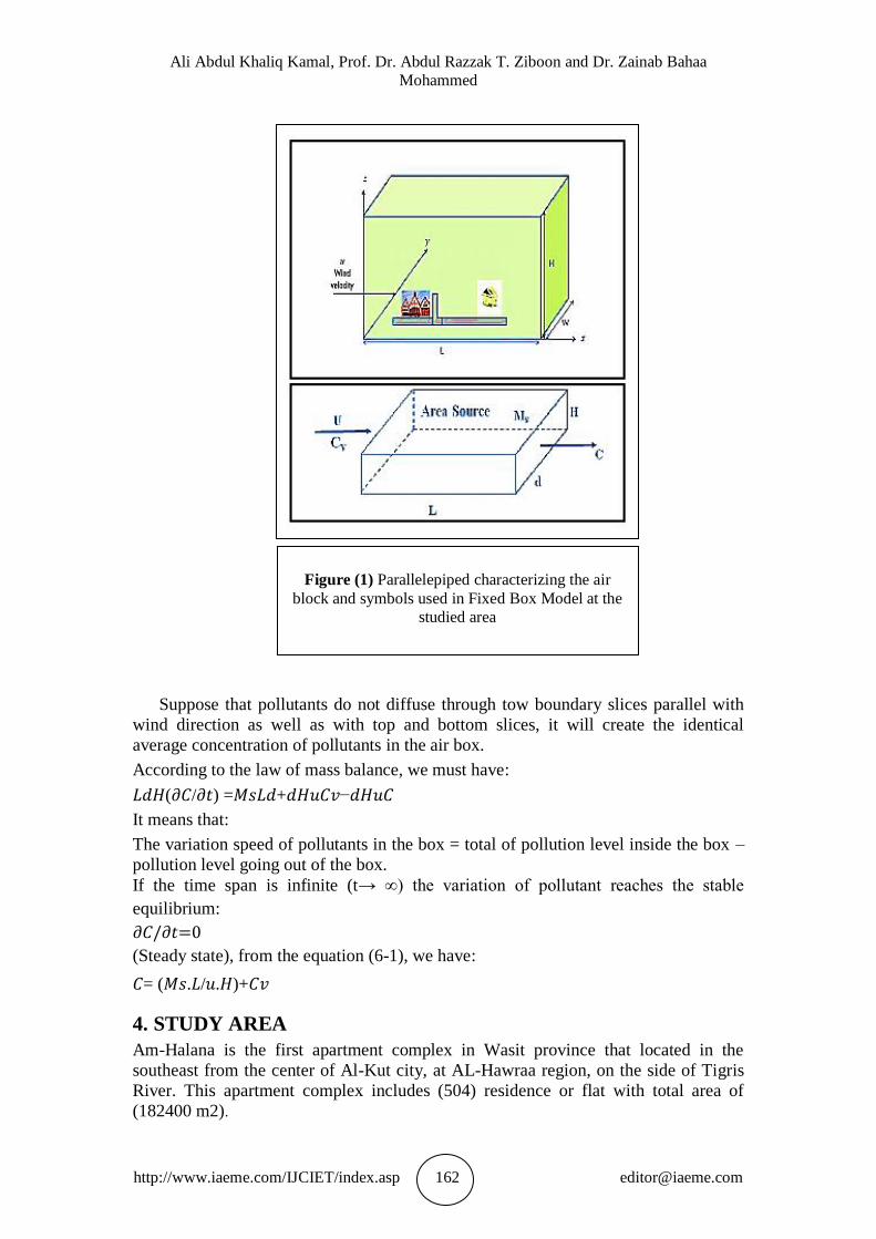
solve a non-steady state problem. Its content is as follows:

Assuming that the air block at the studied area has a parallelepiped shape with length

L (m), width d (m), and height H (m) which is often the height of atmospheric

turbulent mixing layer.

Capacity of area source is Ms (mg/m2.s).

The wind whose direction is perpendicular to the width has the average speed U

(m/s).

The wind takes a pollution flow that has the concentration Cv (mg/m3).

The concentration inside the parallelepiped is equal C (mg/m3) as shown in Figure

(1) below.


Mohammed


Suppose that pollutants do not diffuse through tow boundary slices parallel with

wind direction as well as with top and bottom slices, it will create the identical

average concentration of pollutants in the air box.

According to the law of mass balance, we must have:

( / ) = + −

It means that:

The variation speed of pollutants in the box = total of pollution level inside the box –

pollution level going out of the box.

If the time span is infinite (t→ ∞) the variation of pollutant reaches the stable

equilibrium:

/ =0 (Steady state), from the equation (6-1), we have:

= ( . / . )+

4. STUDY AREA

Am-Halana is the first apartment complex in Wasit province that located in the

southeast from the center of Al-Kut city, at AL-Hawraa region, on the side of Tigris

River. This apartment complex includes (504) residence or flat with total area of

(182400 m2).

Figure (1) Parallelepiped characterizing the air

block and symbols used in Fixed Box Model at the

studied area




This area has been chosen as model for large cities, to controlling the necessary

parameters that needs for the method of fixed box model during the study period.

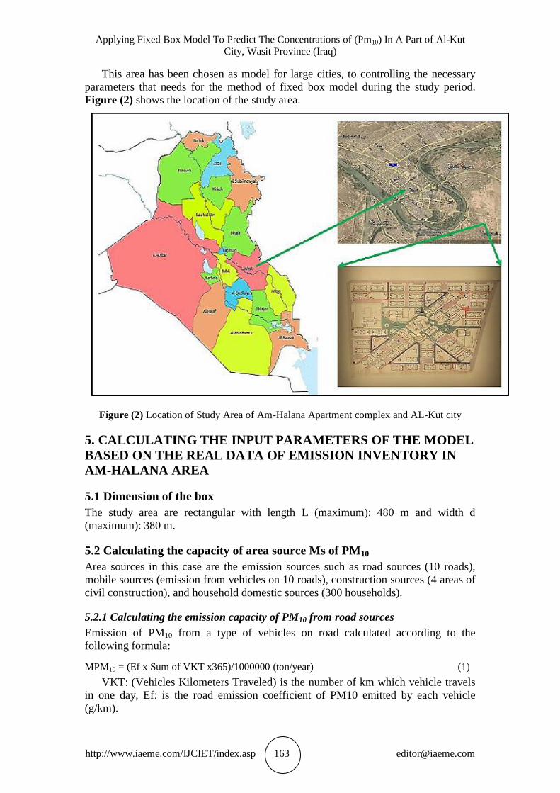
Figure (2) shows the location of the study area.

Figure (2) Location of Study Area of Am-Halana Apartment complex and AL-Kut city

5. CALCULATING THE INPUT PARAMETERS OF THE MODEL

BASED ON THE REAL DATA OF EMISSION INVENTORY IN

AM-HALANA AREA

5.1 Dimension of the box

The study area are rectangular with length L (maximum): 480 m and width d

(maximum): 380 m.

5.2 Calculating the capacity of area source Ms of PM10

Area sources in this case are the emission sources such as road sources (10 roads),

mobile sources (emission from vehicles on 10 roads), construction sources (4 areas of

civil construction), and household domestic sources (300 households).

5.2.1 Calculating the emission capacity of PM10 from road sources

Emission of PM10 from a type of vehicles on road calculated according to the

following formula:

MPM10 = (Ef x Sum of VKT x365)/1000000 (ton/year) (1)

VKT: (Vehicles Kilometers Traveled) is the number of km which vehicle travels

in one day, Ef: is the road emission coefficient of PM10 emitted by each vehicle

(g/km).


Mohammed


In which:

Ef=k (sL/2)0.65(W/3)1.5(1-P/4N) (AP42, EPA, 1999)

K: coefficient considering the dimension of PM (g/km).

SL: quantity of alluvia on the road surface (g/m2) varying from (0 – 300 g/m2).

W: average weight of vehicle (ton).

P: total rainy days in year.

N: number of days in year, N=365 days.

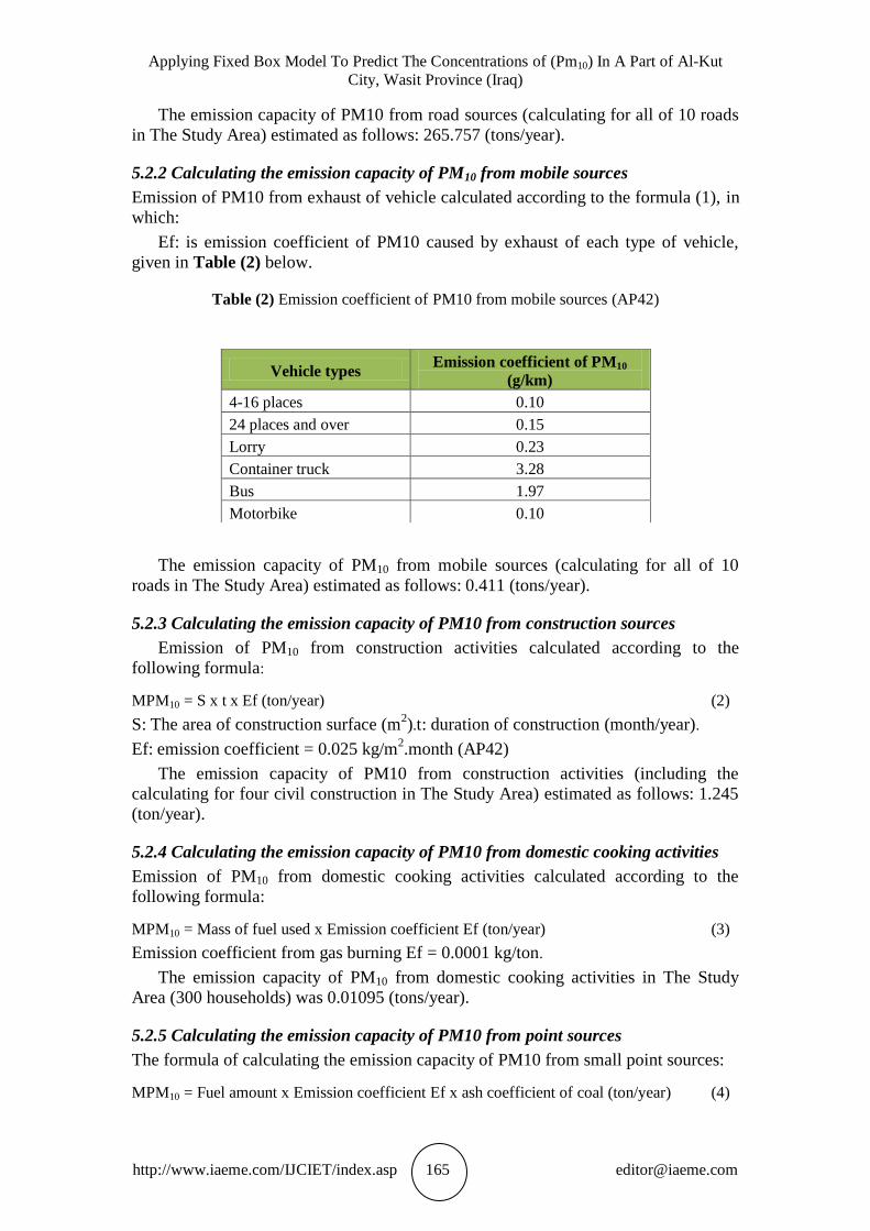
The concretely calculated parameters are in the following table.

Table (1) Parameters of vehicle and parameters related to road source.

Vehicle

type

4-16 places Over 24

places Lorry

Container

truck Bus Motorbike

W (ton) 3 5 5 25 10 0.12

k (PM10) sL P N

4.6 30 51 365

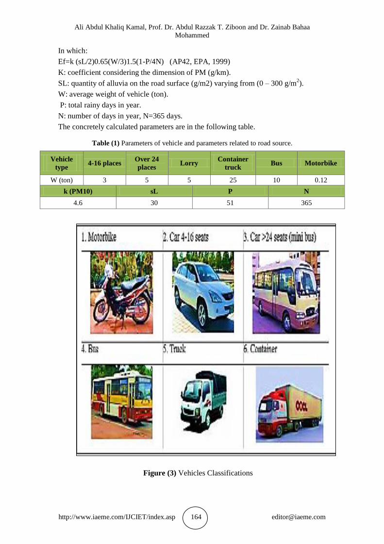
Figure (3) Vehicles Classifications




The emission capacity of PM10 from road sources (calculating for all of 10 roads

in The Study Area) estimated as follows: 265.757 (tons/year).

5.2.2 Calculating the emission capacity of PM10 from mobile sources

Emission of PM10 from exhaust of vehicle calculated according to the formula (1), in

which:

Ef: is emission coefficient of PM10 caused by exhaust of each type of vehicle,

given in Table (2) below.

Table (2) Emission coefficient of PM10 from mobile sources (AP42)

The emission capacity of PM10 from mobile sources (calculating for all of 10

roads in The Study Area) estimated as follows: 0.411 (tons/year).

5.2.3 Calculating the emission capacity of PM10 from construction sources

Emission of PM10 from construction activities calculated according to the

following formula:

MPM10 = S x t x Ef (ton/year) (2)

S: The area of construction surface (m2).t: duration of construction (month/year).

Ef: emission coefficient = 0.025 kg/m2.month (AP42)

The emission capacity of PM10 from construction activities (including the

calculating for four civil construction in The Study Area) estimated as follows: 1.245

(ton/year).

5.2.4 Calculating the emission capacity of PM10 from domestic cooking activities

Emission of PM10 from domestic cooking activities calculated according to the

following formula:

MPM10 = Mass of fuel used x Emission coefficient Ef (ton/year) (3)

Emission coefficient from gas burning Ef = 0.0001 kg/ton.

The emission capacity of PM10 from domestic cooking activities in The Study

Area (300 households) was 0.01095 (tons/year).

5.2.5 Calculating the emission capacity of PM10 from point sources

The formula of calculating the emission capacity of PM10 from small point sources:

MPM10 = Fuel amount x Emission coefficient Ef x ash coefficient of coal (ton/year) (4)

Vehicle types Emission coefficient of PM10

(g/km)

4-16 places 0.10

24 places and over 0.15

Lorry 0.23

Container truck 3.28

Bus 1.97

Motorbike 0.10


Mohammed


The emission capacity of PM10 from small point sources in The Study Area was

zero (ton/year).

6. ADJUSTMENT OF THE CALCULATED RESULTS OF

EMISSION CAPACITY IN THE STUDIED AREA

At present, there is no standard emission coefficient for the above types of studied

sources in the Study Area, United States emission coefficients (according to the

document AP-42, EPA and PUNE project, India, 2004) (PREIS 2004) were used

during the calculating process. Therefore, it is necessary to adjust the calculated

results in order to obtain a relative accuracy. The adjustment principle based on the

surveys of each specific source to correct and estimate the emission capacity M for

the studied area; the results showed in Table (3).

Table (3) Estimation of emission capacities of PM10, from emission sources in the Study Area

with the adjustment coefficient d

Emission sources

Calculated capacity M*

according to document AP-42

and PUNE (ton/year)

Adjustment

coefficient (d)

Adjusted

capacity

(ton/year)

M = M* (d+1)

Civil construction 1.245 0.3 1.6185

Domestic cooking 0.01095 0.15 0.0125

Road source 265.757 0.35 358.7719

Mobile source 0.411 0.15 0.4726

Total 267.4239 360.8755

7. CALCULATION SCENARIOS

7.1. The input parameters of fixed box model based on the Table (3)

Emission capacity of area source Ms = 0.0627 mg/m2.s.

The length of the box = 480 m.

The width of the box = 380 m.

Mixing height: H1= 120 m; H2 = 200 m.

Mixing height is the height H in the atmospheric boundary layer where the

turbulent coefficient Az = Kzζ = const with z > H; of which, Kz is the vertical

turbulent coefficient, ζ is the average density of the studied atmospheric layer.

The researches (Le Dinh Quang, Pham Ngoc Ho 2006) showed that Profile of Az

(or turbulent coefficient Kz) in the atmospheric border layer has a linear dependence

on the distance of vertical movement of turbulent cycle lz= χz (χ- Karman constant ≈

0.4) in the equilibrium condition to the height H=lzmax, corresponding with the




height Zmax varying from (300-500m). Therefore, the height H can be estimated

varies from (120-200m).

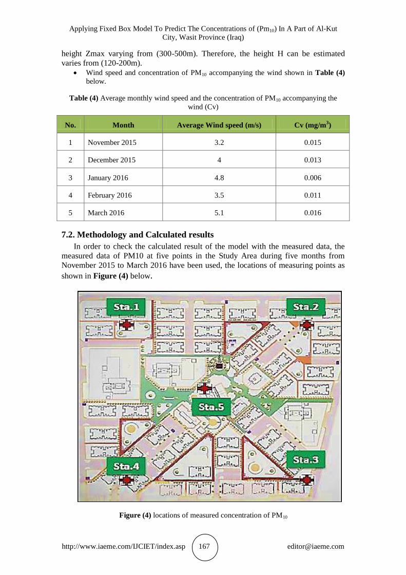
Wind speed and concentration of PM10 accompanying the wind shown in Table (4)

below.

Table (4) Average monthly wind speed and the concentration of PM10 accompanying the

wind (Cv)

No. Month Average Wind speed (m/s) Cv (mg/m3)

1 November 2015 3.2 0.015

2 December 2015 4 0.013

3 January 2016 4.8 0.006

4 February 2016 3.5 0.011

5 March 2016 5.1 0.016

7.2. Methodology and Calculated results

In order to check the calculated result of the model with the measured data, the

measured data of PM10 at five points in the Study Area during five months from

November 2015 to March 2016 have been used, the locations of measuring points as

shown in Figure (4) below.

Figure (4) locations of measured concentration of PM10


Mohammed


The methodology of sampling was 4 times per day at (8 am, 12 pm, 4 pm, and 8

pm). The duration of sampling is (30 min) for each time. The measured data were

averaged for each time, after that they were averaged for all of 4 times to get the

specific values for 24h; and the value of calculated concentration C is considered as

the average concentration of 24h which is taken to compare, the results are indicated

in the Table (5).

Table (5) Comparison between the calculated result of the model and the measured result

(mg/m3)

Month

Measured

concentration

of PM10

(mg/m3)

Calculated

concentration

of the model at

H=120 m

Relative

error (%)

Calculated

concentration

of the model at

H=200 m

Relative

error (%)

November

2015 0.085 0.0783 7.8 0.0470 44.7

December

2015 0.071 0.067 11.7 0.0376 47.1

January

2016 0.055 0.0522 5.1 0.0313 43.1

February

2016 0.079 0.0716 8.1 0.0429 45.7

March 2016

0.51 0.0491 3.7 0.0295 42.2

Table (5) above shows that, the calculated result is closer to the measured result

when (H1 < H2). The calculated results of the model at (H = 120m) where

approximately with relative error below (10%). While the calculated results of the

model at (H = 200m) where all with relative error exceeding (40%). Therefore, the

estimation of mixing height suitable with the actual conditions plays an important

role.

The calculated results from the model that were smaller than the measured results

corresponds with the physical significance because the measured concentration at the

monitoring point is (C = Co + Cv). Of which: (Co) is the calculated concentration of

emission from area sources and (Cv) is the concentration generated by wind flow,

which takes pollutants from other areas into the box (this element has not been

considered yet in the research).

The calculated results from the model also indicate that there has been a scientific

basic for the adjustment in emission inventory and the adjustment has obtained an

acceptable accurate level.

Pollutant’s concentration (Co) is in reverse ratio to wind speed (U) and mixing

height (H) and corresponding to the fixed box length (L) and area source capacity

(Ms).




Compared with the NAAQS and EPA standards (24h average), the concentrations

of PM10 calculated from box model is within the acceptable limits (150 μg/m3) or

(0.15 mg/m3).

The initial result may have significance for studying the application of this fixed

box model on evaluating the air quality in districts of AL-Kut city in particular and

urban areas of Iraq in general.

8. CONCLUSION

This work investigates methodologies for evaluating the performance of dispersion air

quality models. Dispersion models are used to predict the fate of gases and aerosols

after they are released into the atmosphere. The Fixed Box Air Quality Model was

used for studying regional air pollution problem in AL-Kut city. This work has

described a detailed model for studying the urban air pollution.

Mathematical models are needed to optimize air quality monitoring, provide

estimates for monitoring purposes, study different street geometries, and finally test

prospect emission. Depending on their mathematical principles, they may be more or

less suitable for a number of applications. However, validation of the results from this

study for urban air pollution would be highly beneficial. The same approach would

work fit indoors air pollution.

REFERENCES

[1] Daly A, Zannetti P. Air pollution modeling—an overview. In: Zannetti P, Al-

Ajmi D, Al-Rashied S (eds) Ambient air pollution, chapter 2., (2007).

[2] Moussiopoulos N., Studying Atmospheric Pollution in Urban Areas

(SATURN).Subproject of EUROTRAC-2. Project description of March 1997,

which can obtained from Professor Nicolas Moussiopoulos, Aristotle University

Thessaloniki, Box 483, Gr-54006, and Thessaloniki, Greece. Email:

[email protected]. (1997).

[3] Carnevale C, Finzi G, Pisoni E, Thunis P, Volta M. The impact of

thermodynamic module in the CTM performances. Atoms Environ 61:652–660,

(2012).

[4] Tiittanen, P., Timonen, K.L., Ruuskanen, J., Mirme, A., Pekkanen, J., Fine

particulate air pollution, resuspended road dust and respiratory health among

symptomatic children. European Respiratory Journal 12, 266–273, (1999).

[5] Bitan, A., The high climatic quality city of the future. Atmospheric Environment

26B, 313–329, (1992).

[6] Schlink, U., Dorling, S., Pelikan, E., Nunnari, G., Cawley, G., Junninen, H.,

Greig, A., Foxall, R., Eben, K., Chatterto, T., Vondracek, Richter, M., Dostal, M.,

Bertucco, L., Kolehmainen, M., Doyle, M. A rigorous inter-comparison of

ground-level ozone predictions. Atmospheric Environment 37, 3237–3253,

(2003).

[7] Bond, T.C., Zarzycki, C., Flanner, M.G., Koch, D.M. quantifying immediate

radiative forcing by black carbon and organic matter with the specific forcing

pulse. Atmos. Chem. Phys. Discuss. 10, 15713-15753, (2011).

[8] UNEP, Urban Air Quality Management Tool book, UNEP, Nairobi, (2005).

[9] Mahajan, S.P. Air Pollution Control. TERI Press, New Delhi, (2009).

[10] Skouloudis AN. In: Hester RE, Harrison RM, editors. The European auto-oil

programmer: scientific considerations. Environmental science and technology

vol. 8. Royal Society of Chemistry p. 67 – 93, (1997).


Mohammed


[11] Compilation of Air Pollutant Emission Factors (AP-42).

[12] Report of pilot emission inventory in Hanoi, Research Center for Environmental

Monitoring and Modeling (CEMM) and Hanoi Center for Environmental and

Natural Resources Monitoring and Analysis (CENMA), (2008).

[13] Handbook for Criteria Pollutant Inventory Development, EPA-454/R-99-037,

(EPA), (1999).

[14] Kadhim Naief Kadhim and Ahmed Awad Matr Al-Abody, The Geotechnical

Maps For Bearing Capacity by Using Gis and Quality of Ground Water For Al-

Imam District (Babil - Iraq), International Journal of Civil Engineering and

Technology, 6(10), 2015, pp. 176–184.

[15] Kadhim Naief Kadhim, Feasibility of Blending Drainage Water with River Water

For Irrigation In Samawa (Iraq), International Journal of Civil Engineering and

Technology, 4(5), 2013, pp. 22–32.

[16] Mustafa Hamid Abdulwahid and Kadhim Naief Kadhim, Application of Inverse

Routing Methods To Euphrates River (Iraq), International Journal of Civil

Engineering and Technology, 4(1), 2013, pp. 91–109.

applying fixed box model to predict the concentrations...

Documents