applied regression models for longitudinal dataimai.princeton.edu/teaching/files/panel.pdf ·...

Applied Regression Models forLongitudinal Data

Kosuke Imai

Princeton University

Fall 2016POL 573 Quantitative Analysis III

Kosuke Imai (Princeton) Longitudinal Data POL573 (Fall 2016) 1 / 48

Readings

Hayashi, Econometrics, Chapter 5

“Dirty Pool” papers referenced in the slides

Wooldrich, Econometric Analysis of Cross Section and PanelData, Chapter 10 and relevant sections of Part IV

Gelman and Hill, Data Analysis Using Regression andMultilevel/Hierarchical Models, Part 2A, Cambridge UniversityPress.


What Are Longitudinal Data?

Repeated observations for each unitAlso called panel data, cross-section time-series dataAssume balanced data:

Yi︸︷︷︸T×1

=

yi1yi2...

yiT

and Xi︸︷︷︸T×K

=

xi11 xi12 · · · xi1Kxi21 xi22 · · · xi2K

... · · · · · ·...

xiT 1 xiT 2 · · · xiTK

“Stacked” form:

Y︸︷︷︸NT×1

=

Y1Y2...

YN

and X︸︷︷︸NT×K

=

X1X2...

XN


Varying Intercept Models

Basic setup:yit = αi + β>xit + εit

Motivation: unobserved (time-invariant) heterogeneity

yit = α + β>xit + δ>ui + εit

where αi = α + δ>ui

(Strict) Exogeneity given Xi and ui :

E(εit | Xi ,ui) = 0

Constant slopesStatic model: no lagged y in the right hand-side


Fixed-Effects Model

“Fixed” effects mean that αi are model parameters to be estimated(N + K ) parameters to be estimated: inefficient if T is smallHomoskedasticity and independence across time (& units)

V(εi | X) = σ2IT

Stacked vector representation:

Y = Zγ+εwhere D =

1 0 · · · 0...

......

1 0 · · · 00 1 · · · 0...

......

0 0 · · · 1...

......

0 0 · · · 1

, Z = [D X], γ =

α1α2...αNβ


Estimation of Fixed Effects Model

The least-squares estimator (also MLE): γFE = (Z>Z)−1Z>YSampling distribution: γFE | Z ∼ N (γ, σ2(Z>Z)−1)

The dimension of (Z>Z) is large when N is largeComputation based on within-group variation:

Y =

y11 − y1

...yiT − yi

...yNT − yN

and X =

(x11 − x1)>

...(xiT − xi)

>

...(xNT − xN)>

Then, βW = (X>X)−1X>Y and βW | X ∼ N (β, σ2(X>X)−1)


Fixed Effects Estimator as Within-group Estimator

Within-group variation = Residuals from regression of Y on DRecall the geometry of least squares (see Multiple Regressionslides 39 and 43)Projection of Y onto S⊥(D)

Thus, Y = MDY = where MD = INT − D(D>D)−1D>

Also, X = MDXThis is a partitioned regression!

Then, βFE = βW (see Question 1 of POL572 Problem Set 4 ©)Also, ε = Y− ZγFE = Y− XβW

The lower-right block of (Z>Z)−1 equals (X>X)−1

Thus, βW | X ∼ N (β, σ2(X>X)−1)


Kronecker Product

Definition:

An×m ⊗ Bk×l =

a11B a12B . . . a1mBa21B a22B . . . a2mB

......

. . ....

an1B an2B . . . anmB

nk×ml

Some rules (assuming they are conformable):(A⊗ B)> = A> ⊗ B>A⊗ (B + C) = A⊗ B + A⊗ C(A⊗ B)⊗ C = A⊗ (B⊗ C)(A⊗ B)(C⊗ D) = (AC)⊗ (BD)(A⊗ B)−1 = A−1 ⊗ B−1

|A⊗ B| = |A|m|B|n where A and B are n × n and m ×m matrices,respectively.

Fixed effects calculation made easy: D = IN ⊗ 1T which impliesD>D = IN ⊗ (1>T 1T ) = T INPD = D(D>D)−1D> = 1

T IN ⊗ (1T 1>T )


Serial Correlation and Heteroskedasticity

Even after conditioning on xit and ui , yit may still be seriallycorrelatedCorr(εit , εit ′) 6= 0 for t 6= t ′

Independence across units is assumedWe are still assuming we got the conditional mean specificationcorrect and so just need to “fix” standard errorsRobust standard errors (see Multiple Regression slide 24):

V(β | X) = (X>X)−1︸︷︷︸bread

XE(εε> | X)X︸︷︷︸meat

(X>X)−1︸︷︷︸bread

where the “meat” is estimated by∑N

i=1 X>i εi ε>i Xi

Asymptotically consistent with any form of heteroskedasticity andserial correlationCan also use Feasible GLS


Panel Corrected Standard Error

A popular procedure proposed by Beck and Katz (1995)Basic idea: take into account contemporaneous (or spatial)correlation when calculating standard errorsAutocorrelation is assumed to be non-existent

E(εit εit ′ | X) = E(εit εi ′t ′ | X) = 0 for i 6= i ′ and t 6= t ′

Inclusion of lagged dependent variable (more on this later)Spatial correlation is assumed to be time-invariant

ρii ′ = E(εit εi ′t | X) =1T

T∑t ′=1

εit ′ εi ′t ′ for i 6= i ′

These robust standard errors can be applied to any linear models(with or without fixed effects)


A Variety of Exogeneity Assumptions

Contemporaneous exogeneity: E(εit | xit , αi) = 0Not sufficient for identification of β under fixed effects model

Strict exogeneity: E(εit | Xi , αi) = 0Sufficient for identification of β under fixed effects modelerror does not correlate with x at another time

Sequential exogeneity: E(εit | X it , αi) = 0 whereX it = xi1, xi2, . . . , xitpast error can correlate with future x

Dynamic sequential exogeneity: E(εit | X it ,Y i,t−1) = 0 whereY it = yi0, yi1, . . . , yitanalogous to sequential ignorability

Sequential ignorability: yit (1), yit (0) ⊥⊥ xit | X i,t−1,Y i,t−1

sequential randomization, marginal structural models


Fixed Effects and Lagged Dependent Variable

One of the simplest fixed effects model that incorporatesdynamics is the following AR(1) model:

yit = αi + ρyi,t−1 + β>xit + εit where |ρ| < 1

Strict exogeneity does not hold: E(εit | X iT ,Y i,T−1, αi) 6= 0Bias (Nickell) as N goes to∞ with fixed T :

ρ− ρ =

(1

NTY>−1MXY−1

)︸︷︷︸

AT

−1 1NT

Y>ε

p−→ −A−1T ·

σ2

T (1− ρ)

(1− 1− ρT

T (1− ρ)

)β − β = (ρ− ρ)(X>X)−1X>Y−1 + (X>X)−1X>ε

p−→ −A−1T ·

σ2

T (1− ρ)

(1− 1− ρT

T (1− ρ)

)· δ

where (X>X)−1X>Y−1p−→ δ


First Differencing for Identification

The model: yit = αi + ρyi,t−1 + β>xit + εit

Assumption: dynamic sequential exogeneity E(εit | X it ,Y i,t−1) = 0Implies E(εit ) = E(εitεit ′) = 0 for t 6= t ′

First differencing:

∆yit = ρ∆yi,t−1 + β>∆xit + ∆εit

where ∆yit = yit − yi,t−1 etc.Instrumental variables:

Anderson and Hsiao: yi,t−2 or ∆yi,t−2Arellano and Bond: use all instruments with GMM

t = 3: E(∆εi3yi1) = 0t = 4: E(∆εi4yi2) = E(∆εi4yi1) = 0t = 5: E(∆εi5yi3) = E(∆εi5yi2) = E(∆εi5yi1) = 0and so on; a total of (T − 2)(T − 1)/2 instruments

Instruments derived from the model rather than from thequalitative information


Random Effects Model

Dimension reduction is desirable when N is large relative to T“Random” intercepts: a prior distribution on αi

αii.i.d.∼ N (α, ω2)

Additional assumptions:1 A family of distributions for αi2 Independence between αi and X

Reduced form when εiti.i.d.∼ N (0, σ2):

Yi | Xindep.∼ N (α1T + Xiβ, σ

2Στ ) where Στ = IT + τ1T 1>T

and τ = ω2/σ2 or using the stacked form

Y | X ∼ N (Zγ, σ2Ωτ ) where Ωτ = IN ⊗ Στ

and Z = [1 X] and γ = (α, β)


Maximum Likelihood Estimation of RE Model

Likelihood function:

(2π)−NT/2|σ2Ωτ |−1/2 exp− 1

2σ2 (Y− Zγ)>Ω−1τ (Y− Zγ)

The same trick as in linear regression:

(Y− Zγ)>Ω−1τ (Y− Zγ)

= (Y− Zγ − Zγ + Zγ)>Ω−1τ (Y− Zγ − Zγ + Zγ)

= (Y− Zγ)>Ω−1τ (Y− Zγ) + (γ − γ)>Z>Ω−1

τ Z(γ − γ)

where γ = (Z>Ω−1τ Z)−1Z>Ω−1

τ YLog-likelihood function:

−TN2

log(2πσ2)− N2

log |Στ | −1

2σ2

NT σ2 + (γ − γ)>Z>Ω−1

τ Z(γ − γ)

where σ2 = (Y− Zγ)>Ω−1τ (Y− Zγ)/(NT )

Given any value of τ , (γ, σ2) is the MLE of (γ, σ2)


Maximum Likelihood Estimation of τ

Useful identities:

Σ−1τ = IT −

τ

1 + τT1T 1>T = MDi +

1T (1 + τT )

1T 1>T

Ω−1τ = IN ⊗ Σ−1

τ = MD + IN ⊗g(τ)

T1T 1>T

where MD = IN ⊗MDi and g(τ) = 1/(1 + τT )

Thus,

Z>Ω−1τ Z = Z>Z + Z>

(IN ⊗

g(τ)

T1T 1>T

)Z

where the second term equals

g(τ)

T

N∑i=1

Z>i 1T 1>T Zi = g(τ)T Z>Z

where Z is a stacked matrix based on Zi = 1T Z>i 1T


Now the MLE of γ and σ2 can be written as,

γτ = (Z>Z + g(τ)T Z>Z)−1(Z>Y + g(τ)T Z>Y )

σ2τ =

1NT

(ˆε>ˆε+ g(τ)T ˆε>ˆε)

where ˆε = Y− Zγτ and ˆε = Y− Zγτ

Maximize the “concentrated” log-likelihood with respect to τ :

τ = argmaxτ

−N2T log σ2

τ + log(1 + τT )

where |Στ | = 1 + τT


Within-group and Between-group Interpretation

Recall the within-group estimator: βW = (X>X)−1X>YBetween-group estimator: βB = (X>X)−1X>Y where Yi = yi − y ,Xi = (xi − x)>, and

Y︸︷︷︸NT×1

=

1T (y1 − y)...

1T (yN − y)

and X︸︷︷︸NT×K

=

1T (x1 − x)>

...1T (xN − x)>

Random effects estimator as the weighted average:

αRE = y − β>RE x

βRE = (X>X + g(τ)X>X)−1(X>XβW + g(τ)X>XβB)

g(τ)→ 0 when T →∞ or τ →∞Asymptotically, βRE ∼ N (β, σ2(X>X + g(τ)X>X)−1)

Under random effects model

V(βRE | X) ≈ σ2(X>X + g(τ)X>X)−1 ≤ V(βW | X) ≈ σ2(X>X)−1


Shrinkage and BLUP

Estimation of varying intercepts under the random effects modelEmpirical Bayes approach:

Bayes: likelihood + subjective priorEmpirical Bayes: likelihood + “objective” prior (estimated from data)

The posterior of αi

N(

τT1 + τT

(yi − β>xi) +1

1 + τTα,

σ2τ

1 + τT

)Plug in αRE , βRE , τ , σ

2 to obtain αi and its confidence interval

αi,RE is the BLUP (Best Linear Unbiased Predictor) without thedistributional assumption for αiShrinkage (partial pooling): weighted average of within-groupmean and overall mean where the weight is a function of T and τ

Borrowing strength: key idea for multilevel/hierarchical models,variable selection (ridge regression, LASSO, etc.)Bias-variance tradeoff


Fixed or Random Intercepts?

Dilemma: Random effects impose additional assumptions but canbe more efficient if the assumptions are correct

Hausman specification test1 Test statistic

H ≡ (βw − βRE )>V(βW − βRE | X)−1(βw − βRE )

= (βw − βRE )>V(βW | X)− V(βRE | X)−1(βw − βRE )

Hausman shows that asymptotically (βW − βRE ) ⊥⊥ βRE2 Null hypothesis: random effects model3 Asymptotic reference distribution: H ∼ χ2

K

Warning: the alternative hypothesis is that random effects modelis wrong but fixed effects model is correct, but in practice bothmodels could be wrong!


Hausman Test Proof

Lemma: Consider two consistent and asymptotically normalestimators of β and call them β0 and β1. Suppose β0 attains theCramer-Rao lower bound. Then, Cov(β0, q) converges asymptoticallyto zero where q = β0 − β1.

1 Define a new estimator β2 = β0 + rAq where r is a scalar and A isan arbitrary matrix to be chosen later

2 Show that β2p→ β with the asymptotic variance

V(β2) = V(β0) + 2rACov(q, β0) + r2AV(q)A>

3 Consider F (r) = V(β2)− V(β0) ≥ 0

4 Choose A = −Cov(q, β0)> and show that F (r) < 0 for a smallvalue of r , which yields a contradiction unless Cov(q, β0) = 0

5 Finally, V(β1) = V(q + β0) = V(q) + V(β0)


An Example: Democratic Peace Debate

International Organizationspecial issueGreen et al., Oneal &Russett, Beck & Katz, King

Dyadic analysisEffect of Democracy onbilateral trade (given here)and conflict (see later slide)Hausman test for pooledanalysis vs. fixed effects

452 International Organization

TABLE 2. Alternative regression analyses of bilateral trade (1951-92)

Pooled with Fixed effects Variable" Pooled Fixed effects dynamics with dynamics

GDP 1.182** 0.810** 0.250** 0.342** (0.008) (0.015) (0.006) (0.013)

Population -0.386** 0.752** -0.059** 0.143* (0.010) (0.082) (0.006) (0.068)

Distance -1.342** Dropped: no -0.328** Dropped: no within-group within-group variation variation

(0.018) (0.012) Alliance -0.745** 0.777** -0.247** 0.419**

(0.042) (0.136) (0.027) (0.121) Democracyb 0.075** -0.039** 0.022** -0.009**

(0.002) (0.003) (0.001) (0.002) Lagged 0.736** 0.533**

bilateral trade (0.002) (0.003) Constant -17.331** -47.994** -3.046** -13.745**

(0.265) (1.999) (0.177) (1.676) N = 93,924 NT = 93,924 N = 88,946 NT= 88,946

N = 3,079 N= 3,079 T 20 T 20

Adjusted R2 0.36 0.63 0.73 0.76

Note: Estimates obtained using areg and xtreg procedures in STATA, version 6.0. aGDP, population, distance, and bilateral trade are natural-log transformed. Method of analysis is

OLS and fixed-effects regression. bLower value within the dyad. **p < .01.

*p < .05, two-tailed test.

trade volume but lacks firm theoretical foundation.18 Political scientists have treated the gravity model as something of a baseline, appending additional political variables. We follow current practice in the spirit of examining the consequences of different modeling assumptions. We include as regressors the democracy and alliance measures from the previous analysis. Table 2 presents both pooled and fixed-effects models, each with and without a lagged dependent variable as a

regressor. We find no support whatsoever for the null hypothesis that all dyads share the same intercept. For the nondynamic case, F(3078,90841) - 23.68, p < .0001; when lagged trade is introduced as an independent variable, F(3078, 85862) = 4.43, p < .0001.

Clearly, the dyads have different intercepts, but are these omitted intercepts a source of bias for pooled regression? The correlation between the dyad-specific

18. Bergstrand 1985, 474.


A Generalization of Random Effects Model

Random effects model assumes αi ⊥⊥ Xi“Correlated” random effects:

αi | Xiindep.∼ N (α + ξ>xi , ω

2)

Then, β>xit + ξ>xi = β>(xit − xi) + (β + ξ)>xi implies

Zi =

1 (xi1 − xi)> x>i

......

...1 (xiT − xi)

> x>i

and γ =

αβλ

where λ = β + ξ

This leads to the surprising result:

βCRE = βW and λCRE = βB

Empirical Bayes estimate of αi :τT

1 + τTαi,FE +

11 + τT

(y − β>B x + (βB − βW )>xi)


Models with Varying Slopes and Intercepts

Random effects model can be made richer and more flexibleLinear mixed effects models:

Yi | X,Z, ζindep.∼ N (Xiβ + Ziζi , Σi)

ζi | X,Zi.i.d.∼ N (0,Ω)

where Z is typically a subset of XEstimating ζi without partial pooling is unrealistic when thedimension of Zi is largeUseful if intercepts/slopes differ across units and are of interestMultilevel/hierarchical models are extensions of this basic model(see Gelman and Hill (2007) for many interesting examples)Reduced form:

Yi | X,Zindep.∼ N (Xiβ, Λi)

where Λi = ZiΩZ>i + Σi


Estimation of Linear Mixed Effects Models

With known variance, the GLS is the MLE:

β =

(N∑

i=1

X>i Λ−1i Xi

)−1 N∑i=1

X>i Λ−1i Yi

Empirical Bayes estimate for ζi :

ζi = (Z>i Σ−1i Zi + Ω−1)−1Z>i Σ−1

i (Yi − Xi β)

= ΩZ>i Λ−1i (Yi − Xi β)

For known variance, ζi attains the smallest MSERestricted Maximum Likelihood (REML) to estimate variancewhere β is integrated out from the likelihood over improper priorlmer() in the lme4 package

Possible to obtain the MLE of all parameters at once via the EMalgorithm treating ζi as missing dataFully Bayesian approach via Gibbs sampling


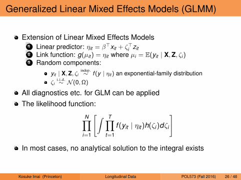
Generalized Linear Mixed Effects Models (GLMM)

Extension of Linear Mixed Effects Models1 Linear predictor: ηit = β>xit + ζ>i zit2 Link function: g(µit ) = ηit where µi = E(yit | X,Z, ζi )3 Random components:

yit | X,Z, ζiindep.∼ f (y | ηit ) an exponential-family distribution

ζii.i.d.∼ N (0,Ω)

All diagnostics etc. for GLM can be appliedThe likelihood function:

N∏i=1

[∫ T∏t=1

f (yit | ηit )h(ζi)dζi

]

In most cases, no analytical solution to the integral exists


Estimation of GLMM

Decomposition: yit = g−1(ηit ) + εit

Taylor expansion around current estimates (β(t), ζ(t)):

Y (t)i ≈ Xiβ+Ziζi+ε

(t)i where Y (t)

i = (V (t)i )−1(Yi−µi)+Xi β

(t)+Zi ζ(t)i

where Vi is the diagonal matrix whose diagonal elementcorresponds the variance function b′′(µit )

Iterated Weighted Least Squares where each iteration involves theoptimization problem under a linear mixed effects model

The resulting estimator can be justified as the penalizedquasi-likelihood estimatorThe approximation can be poorAlternative approximation: Gaussian quadrature (glmer())MCEM and MCMC


An Example: Modeling Latent Social Networks

Hoff and Ward (Political Analysis, 2004)Modeling bilateral trade using cross-section dyadic dataModel (export from i to j)

yij = β>xij + ai + bj + γij + z>i zj︸︷︷︸εij

where ai is the sender effect, bj is the receiver effect, γij is thedyadic effect, zi is a vector in the latent network spaceRandom effects specification

1 (ai ,bi ) ∼ N (0,Σ)2 γij = γji ∼ N (0,Φ)3 zi ∼ N (0, σ2I)


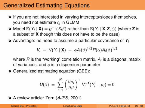
Generalized Estimating Equations

If you are not interested in varying intercepts/slopes themselves,you need not estimate ζi in GLMMModel E(Yi | X) = g−1(Xiβ) rather than E(Yi | X,Z, ζi) (where Z isa subset of X though this does not have to be the case)Advantage: no need to assume a particular covariance of Yi

Vi = V(Yi | X) = φAi(β)1/2R(α)Ai(β)1/2

where R is the “working” correlation matrix, Ai is a diagonal matrixof variances, and φ is a dispersion parameterGeneralized estimating equation (GEE):

U(β) =N∑

i=1

(∂µi

∂β

)>V−1

i (Yi − µi) = 0

A review article: Zorn (AJPS, 2001)


Properties of GEE

Close connection to the Method of MomentsAsymptotic properties hold even when R(α) is misspecified(consistency and normality with robust standard error)

√N(βN − β0)

D−→ N(

0,E(D>i V−1i Di )

−1E(D>i V−1i V(Yi | X)V−1

i Di )E(D>i V−1i Di )

−1)

where Di is ∂µi/∂β

Advantages of GEE1 Only need to get the mean right! (most efficient when you get the

variance structure correct)2 Unlike the independence model with robust standard error, you get

consistency as well as asymptotic normality3 Possible efficiency gain by accounting for correlation in the data

GEE does assume exogeneity: you need to get the mean correct


Working Correlation Matrix and Estimation of GEE

Popular choices:1 Independence: Ri (t , t ′) = 02 Exchangeability: Ri (t , t ′) = α3 AR(1): Ri (t , t ′) = α|t−t′|

4 Stationary m-dependence: Ri (t , t ′) =

αt,t′ if |t − t ′| ≤ m

0 otherwise5 Unstructured: Ri (t , t ′) = αt,t′

Iterative estimation procedure1 Use β(t) to update Di and Ai2 Estimate V(Yi | X)(t) =

∑Ni=1(Yi − µ(t))>(Yi − µ(t))/N

3 Compute Pearson residuals εPit and estimateφ(t) =

∑Ni=1∑T

t=1(εPit )2/NT and R(α(t)), which give V (t)i

4 Update β using one iteration of Fisher-scoring algorithm

β(t+1) = β(t) −

n∑

i=1

(D(t)i )>(V (t)

i )−1D(t)i

−1 n∑i=1

D(t)i (V (t)

i )−1(Yi − µ(t))


Fixed Effects in GLM

Model:E(yit | X) = g−1(β>xit + αi)

Incidental parameter problem (Neyman and Scott):# of parameters goes to infinity as N tends to infinity (for fixed T )Asymptotic properties of MLE are no longer guaranteed to holdEspecially problematic for small T and large N

In the linear case, everything is fine because the samplingdistribution of β does not depend on αi

In the nonlinear case, this is not generally the caseCanonical example: fixed effects logistic regression with T = 2and xit = time dummy

Model: Pr(yit = 1 | X) = exp(αi+βxit )1+exp(αi+βxit )

αi =

∞ if (yi1, yi2) = (1,1)−∞ if (yi1, yi2) = (0,0)

βP→ 2β


Conditional Likelihood Inference

Maximize conditional likelihood given a sufficient statistic for αiS(Y ) is said to be a sufficient statistic for θ if the conditionaldistribution of Y given S(Y ) does not depend on θProperties (Andersen): asymptotically consistent and normal, lessefficient than MLEA simple example:

yit = β>xit + αi + εit where εiti.i.d.∼ N (0, σ2)

Sufficient statistic for αi is∑T

t=1 yitConditional likelihood function:

N∏i=1

f

(yi1, . . . , yiT

∣∣∣ xit ,

T∑t=1

yit

)

∝ exp

[− 1

2σ2

N∑i=1

(T∑

t=1

(yit − yi)− β>(xit − xi)

2)]


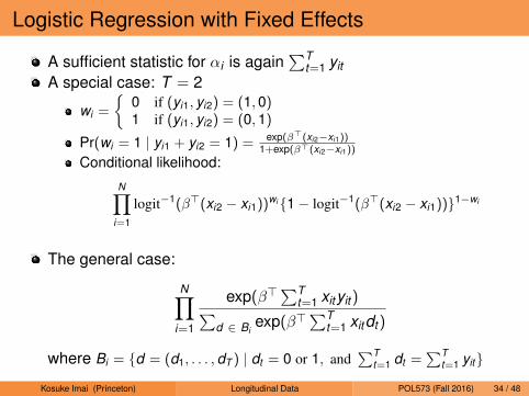
Logistic Regression with Fixed Effects

A sufficient statistic for αi is again∑T

t=1 yitA special case: T = 2

wi =

0 if (yi1, yi2) = (1,0)1 if (yi1, yi2) = (0,1)

Pr(wi = 1 | yi1 + yi2 = 1) = exp(β>(xi2−xi1))1+exp(β>(xi2−xi1))

Conditional likelihood:

N∏i=1

logit−1(β>(xi2 − xi1))wi1− logit−1(β>(xi2 − xi1))1−wi

The general case:

N∏i=1

exp(β>∑T

t=1 xityit )∑d ∈ Bi

exp(β>∑T

t=1 xitdt )

where Bi = d = (d1, . . . ,dT ) | dt = 0 or 1, and∑T

t=1 dt =∑T

t=1 yit


Estimation and Conditional Likelihood

Equivalent to the partial likelihood function of the stratified Coxmodel in discrete time

Single discrete time period (rather than continuous)All observations with yit = 1 are considered as failures at time 1All observations with yit = 0 are considered as censored at time 1Units correspond to strata

In R, you use the following syntax or clogit():coxph(Surv(time = rep(1, N*T), status = y) ~

x + strata(units), method = "exact")

The exact calculation can be difficult when the number of timeperiods is large; use approximation


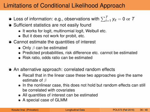
Limitations of Conditional Likelihood Approach

Loss of information: e.g., observations with∑T

t=1 yit = 0 or TSufficient statistics are not easily found

It works for logit, multinomial logit, Weibull etc.But it does not work for probit, etc.

Cannot estimate the quantities of interestOnly β can be estimatedPredicted probabilities, risk difference etc. cannot be estimatedRisk ratio, odds ratio can be estimated

An alternative approach: correlated random effectsRecall that in the linear case these two approaches give the sameestimate of βIn the nonlinear case, this does not hold but random effects can stillbe correlated with covariatesAll quantities of interest can be estimatedA special case of GLMM


Back to Dirty Pool

Democratic Peace: Effect ofDemocracy on militarizeddisputesHausman test for pooledanalysis vs. fixed effectsConditional likelihood:Peaceful dyads are droppedWhat is the effect size?Oneal and Russett estimatepositive effects using fixedeffects model for the datafrom 1885 (instead of 1952)Heterogeneous effects?

454 International Organization

TABLE 3. Alternative logistic regression analyses of militarized interstate disputes (1951-92)

Pooled with Fixed effects Variable Pooled Fixed effects dynamics with dynamics

Contiguity 3.042** 1.902** 1.992** 1.590** (0.092) (0.336) (0.120) (0.375)

Capability ratio 0.102** 0.387** 0.125** 0.350* (log) (0.024) (0.139) (0.028) (0.151)

Growtha -0.017 -0.059** -0.026* -0.062** (0.011) (0.012) (0.013) (0.013)

Alliance -0.234* -1.066* -0.013 -1.090* (0.097) (0.426) (0.118) (0.526)

Democracya -0.057** -0.003 -0.053** 0.0004 (0.007) (0.015) (0.008) (0.016)

Bilateral -0.194* -0.072 0.028 0.084 trade/GDPa (0.087) (0.186) (0.075) (0.217)

Lagged dispute 4.940** 1.813** (0.102) (0.103)

Constant -5.809** -6.274** (0.090) (0.108)

N 93,755 93,755b 88,752 88,752C Log likelihood -3,688.06 -1,546.53 -2,530.31 -1,299.53 x2 1,186.43 75.75 3,074.67 380.40 Degrees of freedom 6 6 7 7 Prob > 2 <0.0001 <0.0001 <0.0001 <0.0001

Note: Estimates obtained using logit and clogit procedures in STATA, version 6.0. aLower value within the dyad. Method of analysis: Logistic and fixed-effects logistic regression. b2,877 groups (87,402 observations) have no variation in outcomes. C2,883 groups (82,932 observations) have no variation in outcomes. **p < .01. *p < .05, two-tailed test.

assumptions implicit in different regression models greatly shape how one thinks about the determinants of bilateral trade.

To illustrate further the importance of fixed effects, we turn our attention to a nonlinear estimation problem. Table 3 reports the results of alternative logistic- regression models of militarized disputes. The pooled analysis suggests that the likelihood of disputes increases when dyads are contiguous and decreases as the less-democratic member of the dyad becomes more democratic. Alliances decrease the risk of war, whereas differences in military capabilities increase it. These results are in line with published research.

These estimates change markedly when fixed effects are controlled. Democracy's effects become negligible and statistically insignificant, whereas military capability and alliance prove much more influential. Consider, for example, what the fixed- effects regression results tell us about a dyad with a 5 percent chance of war. If the


Modeling Dynamics

Previous approaches: treating dynamics as a nuisanceIf dynamics are of substantive interest, they should be modeledDynamic linear models (DLMs):

yitindep.∼ N (X>it β + Z>it γt , σ

2)

where time-varying coefficients γt has a random-walk prior,

γtindep.∼ N (γt−1, Σ)

for t = 2, . . . ,T and γ1 ∼ N (µ0,Ω0)

Can add the second level covariates: γtindep.∼ N (Vtγt−1,Σ)

A special case of state-space models and Markov models


Dependence through the Simple Markov Structure

γ1 γ2 γ3

Y1 Y2 Y3


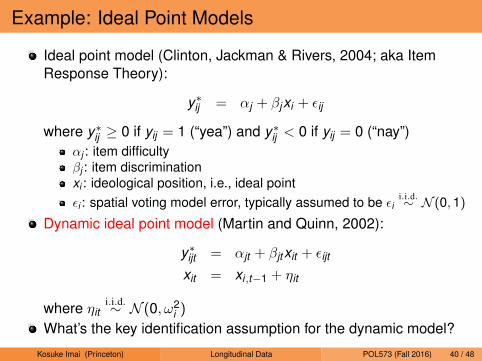
Example: Ideal Point Models

Ideal point model (Clinton, Jackman & Rivers, 2004; aka ItemResponse Theory):

y∗ij = αj + βjxi + εij

where y∗ij ≥ 0 if yij = 1 (“yea”) and y∗ij < 0 if yij = 0 (“nay”)αj : item difficultyβj : item discriminationxi : ideological position, i.e., ideal pointεi : spatial voting model error, typically assumed to be εi

i.i.d.∼ N (0,1)

Dynamic ideal point model (Martin and Quinn, 2002):

y∗ijt = αjt + βjtxit + εijt

xit = xi,t−1 + ηit

where ηiti.i.d.∼ N (0, ω2

i )

What’s the key identification assumption for the dynamic model?


Estimated Ideal Points for Supreme Court Justices

P1: FIC

OJ002-04 April 12, 2002 16:23

148 Andrew D. Martin and Kevin M. Quinn

Fig. 1 Posterior density summary of the ideal points of selected justices for the terms in which theyserved for the dynamic ideal point model.

Similarly, they find trends for Warren, Clark, and Powell that we do not. By controlling forcase stimuli and accounting for estimation uncertainty, we reach substantively very differentconclusions.

We might also be interested in the posterior probability that a given justice’s ideal pointin one term is greater than that justice’s ideal point in another term. This quantity is easilycalculated from the MCMC output. As an illustration, we compute the posterior probability


EM Algorithm for DLM

Complete-data likelihood function:

p(Y, γ | X,Z;β, σ2,Σ, µ0,Ω0)

= p(γ1;µ0,Ω0)T∏

t=2

p(γt | γt−1; Σ)T∏

t=1

p(Yt | Xt ,Zt , γt ;β, σ2)

where Ytindep.∼ N (Xtβ + Ztγt , σ

2IN)

EM updates:1 µ0 = E(γ1) and Ω0 = E(γ1γ

>1 )− E(γ1)E(γ1)>

2 Σ = 1T−1

∑Tt=2

E(γtγ

>t )− E(γtγ

>t−1)− E(γt−1γ

>t ) + E(γt−1γ

>t−1)

3 β = (

∑Tt=1 X>t Xt )

−1∑Tt=1 X>t Yt − ZtE(γt )

4 σ2 = 1T

∑Tt=1∑N

i=1y2it − 2yitZ>it E(γt ) + Z>it E(γtγ

>t )Zit

where yit = yit − X>it β


Computation for E-step

Must compute E(γt ), E(γtγ>t ) and E(γtγ

>t−1) conditional on all data

Define

α(γt ) = p(γt | Y1, . . . ,Yt )

δ(γt ) = p(Yt+1, . . . ,YT | γt )

The posterior is given by,

p(γt | Y1, . . . ,YT ) = ct α(γt ) δ(γt )

where ct = 1/p(Yt+1, . . . ,YT | Y1, . . . ,Yt ) is a normalizingconstant

The joint distribution of (Y1, . . . ,YT ) and (γ1, . . . , γT ) is Gaussianα(γt ), δ(γt ), and α(γt )δ(γt ) are all Gaussian

Forward-backward algorithm thorough Kalman filtering


Forward Recursion

α(γt ) =

∫p(γt , γt−1 | Y1, . . . ,Yt ) dγt−1

=

∫p(γt , γt−1,Yt | Y1, . . . ,Yt−1)

p(Yt | Y1, . . . ,Yt−1)dγt−1

∝∫

p(Yt , γt | γt−1,Y1, . . . ,Yt−1) p(γt−1 | Y1, . . . ,Yt−1) dγt−1

∝ p(Yt | γt )

∫p(γt | γt−1) α(γt−1) dγt−1

Thus, α(γt ) = N (µt ,Ωt ) is obtained as,

φ(γt ;µt ,Ωt )

∝ φ(Yt ; Xtβ + Ztγt , σ2I)∫φ(γt ; γt−1,Σ)φ(γt−1;µt−1,Ωt−1) dγt−1

∝ φ(Yt ; Xtβ + Ztγt , σ2I) φ(γt ;µt−1,Qt−1)

where Qt−1 = Ωt−1 + Σ.Kosuke Imai (Princeton) Longitudinal Data POL573 (Fall 2016) 44 / 48

Finally, Bayes rule gives,

µt = Ωt (Q−1t−1µt−1 + σ−2Z>t Yt )

Ωt = (Q−1t−1 + σ−2Z>t Zt )

−1

We can further simplify using the Woodbury formula,

(A + BD−1C)−1 = A−1 − A−1B(D + CA−1B)−1CA−1

which implies

Ωt = Qt−1 −Qt−1Z>t (σ2I + ZtQt−1Z>t )−1ZtQt−1

= (I− RtZt )Qt−1

where Rt = Qt−1Z>t (σ2I + ZtQt−1Z>t )−1. Finally, note another rule:

(A−1 + B>C−1B)−1B>C−1 = AB>(BAB> + C)−1

Then, we have

ΩtZ>t σ−2I = Qt−1Z>t (ZtQt−1Z>t + σ2I)−1 = Rt

µt = µt−1 + Rt (Yt − Ztµt−1)


Backward Recursion

p(γt | Y1, . . . ,YT ) =

∫p(γt , γt+1 | Y1, . . . ,YT ) dγt+1

=

∫p(γt | γt+1,Y1, . . . ,Yt )p(γt+1 | Y1, . . . ,YT ) dγt+1

From the forward recursion, we have,(γt+1γt

)| Y1, . . . ,Yt ∼ N

((µtµt

),

(Γt + ω2

x ΓtΓt Γt

))Then, the conditional distribution is given by,

γt | γt+1,Y1, . . . ,YT

∼ N (µt + Γt (Γt + ω2x )−1(γt+1 − µt ), Γt − Γt (Γt + ω2

x )−1Γt )


Concluding Remarks

Longitudinal data: opportunities to model within-unit andacross-time variation as well as across-unit variationOld debates: fixed or random interceptsGLMM: a generalization of random effects modelsModel slopes as well as intercepts: importance of substantivetheoryStructural modeling and causal inferenceFor causal inference, getting the conditional mean right isessentialStatic models ignore the systematic dependence on pastoutcomes: all dependence is in the error term


applied regression models for longitudinal dataimai.princeton.edu/teaching/files/panel.pdf ·...

Documents