applied high performance computing using...
TRANSCRIPT

Diploma Thesis
Applied High Performance ComputingUsing R
Stefan Theußl
27.09.2007
Supervisor: univ. Prof. Dipl. Ing. Dr. Kurt Hornik
Department of Statistics and MathematicsVienna University of Economics and Business Administration
Augasse 2-6A-1090 Vienna

Abstract
Applied High Performance Computing
Using R
In the 1990s the Beowulf project smoothed to way for massively paral-lel computing as access to parallel computing power became affordable forresearch institutions and the industry. But the massive breakthrough ofparallel computing has still not occurred. This is because two things weremissing: low cost parallel computers and simple to use parallel programmingmodels. However, with the introduction of multicore processors for main-stream computers and implicit parallel programming models like OpenMPa fundamental change of the way developers design and build their softwareapplications is taken place—a change towards parallel computing.
This thesis gives an overview of the field of high performance computingwith a special focus on parallel computing in connection with the R environ-ment for statistical computing and graphics. Furthermore, an introductionto parallel computing using various extensions to R is given.
The major contribution of this thesis is the package called paRc, whichcontains an interface to OpenMP and provides a benchmark environment tocompare various parallel programming models like MPI or PVM with eachother as well as with highly optimized (BLAS) libraries. The dot productmatrix multiplication was chosen as the benchmark task as it is a primeexample in parallel computing.
Eventually a case study in computational finance is presented in thisthesis. It deals with the pricing of derivatives (European call options) usingparallel Monte Carlo simulation.
Kurzfassung
Angewandtes Hochleistungsrechnen unter
Verwendung von R
In den 1990er Jahren ebnete das Beowulf Projekt den Weg fur massivesParallelrechnen, weil dadurch der Zugang zu parallelen Rechenresourcen furviele Forschungsinstitute und der Industrie erst leistbar wurde. Trotzdemwar der große Durchbruch lange nicht erkennbar. Ausschlaggebend dafurwaren zwei Aspekte: Erstens gab es bisher keine gunstigen Parallelrech-ner und zweitens waren auch keine einfachen Parallelprogrammiermodelle
i
vorhanden. Die Einfuhrung von Multicoreprozessoren fur Desktopsystemeund impliziter Programmiermodelle wie OpenMP fuhrte zu einem Umbruch,der auch Auswirkungen auf die Softwareentwicklung hat. Der Trend gehtdabei immer mehr in Richtung Parallelrechnen.
Diese Diplomarbeitet bietet einen Uberblick uber das Feld des Hochleis-tungsrechnens und im Speziellen des Parallelrechnens unter Verwendung vonR, einer Softwareumgebung fur statistisches Rechnen und Grafiken. Daruber-hinaus beinhaltet diese Arbeit eine Einfuhrung in paralleles Rechnen unterVerwendung mehrerer Erweiterung zu R.
Der Kern dieser Arbeit ist die Entwicklung eines Paketes namens paRc.Diese Erweiterung beinhaltet eine Schnittstelle zu OpenMP und stellt eineBenchmark Umgebung zur Verfugung, mit der verschiedene Parallelepro-grammiermodelle wie MPI oder PVM sowie hochoptimierte Bibliotheken(BLAS) miteinander verglichen werden konnen. Als Aufgabe fur diese Bench-marks wurde das klassische Beispiel aus dem Bereich des Parallelrechnens,namlich die Matrix Multiplikation, gewahlt.
Schlussendlich wird in dieser Arbeit eine Fallstudie aus der computa-tionalen Finanzwirtschaft prasentiert. Im Mittelpunkt dieser Fallstudie stehtdie Bewertung von Derivaten (Europaische Call Optionen) unter Verwendungparalleler Monte Carlo Simulation.
ii

Contents
1 Introduction 11.1 Motivation . . . . . . . . . . . . . . . . . . . . . . . . . . . . . 11.2 Contributions . . . . . . . . . . . . . . . . . . . . . . . . . . . 21.3 Organization of this Thesis . . . . . . . . . . . . . . . . . . . . 2
2 Parallel Computing 32.1 Introduction . . . . . . . . . . . . . . . . . . . . . . . . . . . . 32.2 Terms and Definitions . . . . . . . . . . . . . . . . . . . . . . 5
2.2.1 Process vs. Thread . . . . . . . . . . . . . . . . . . . . 52.2.2 Parallelism vs. Concurrency . . . . . . . . . . . . . . . 52.2.3 Computational Overhead . . . . . . . . . . . . . . . . . 62.2.4 Scalability . . . . . . . . . . . . . . . . . . . . . . . . . 7
2.3 Computer Architecture . . . . . . . . . . . . . . . . . . . . . . 72.3.1 Beyond Flynn’s Taxonomy . . . . . . . . . . . . . . . . 72.3.2 Processor and Memory . . . . . . . . . . . . . . . . . . 92.3.3 High Performance Computing Servers . . . . . . . . . . 11
2.4 MIMD Computers . . . . . . . . . . . . . . . . . . . . . . . . 132.4.1 Shared Memory Systems . . . . . . . . . . . . . . . . . 142.4.2 Distributed Memory Systems . . . . . . . . . . . . . . 14
2.5 Parallel Programming Models . . . . . . . . . . . . . . . . . . 162.5.1 Fundamentals of Message Passing . . . . . . . . . . . . 172.5.2 The Message Passing Interface (MPI) . . . . . . . . . . 182.5.3 Parallel Virtual Machine (PVM) . . . . . . . . . . . . . 202.5.4 OpenMP . . . . . . . . . . . . . . . . . . . . . . . . . . 21
2.6 Design of Parallel Programs . . . . . . . . . . . . . . . . . . . 232.6.1 Granularity of Parallel Programs . . . . . . . . . . . . 232.6.2 Organization of Parallel Tasks . . . . . . . . . . . . . . 242.6.3 Types of Achieving Parallelism . . . . . . . . . . . . . 25
2.7 Performance Analysis . . . . . . . . . . . . . . . . . . . . . . . 262.7.1 Execution Time and Speedup . . . . . . . . . . . . . . 262.7.2 Amdahl’s Law . . . . . . . . . . . . . . . . . . . . . . . 26
iii

2.8 Hardware and Software Used . . . . . . . . . . . . . . . . . . . 272.8.1 High Performance Computing Servers . . . . . . . . . . 272.8.2 Utilized Software . . . . . . . . . . . . . . . . . . . . . 29
2.9 Conclusion . . . . . . . . . . . . . . . . . . . . . . . . . . . . . 30
3 High Performance Computing and R 313.1 Introduction . . . . . . . . . . . . . . . . . . . . . . . . . . . . 313.2 The R Environment . . . . . . . . . . . . . . . . . . . . . . . . 313.3 The Rmpi Package . . . . . . . . . . . . . . . . . . . . . . . . 32
3.3.1 Initialization and Status Queries . . . . . . . . . . . . . 333.3.2 Process Spawning and Communication . . . . . . . . . 343.3.3 Built-in High Level Functions . . . . . . . . . . . . . . 363.3.4 Other Important Functions . . . . . . . . . . . . . . . 373.3.5 Conclusion . . . . . . . . . . . . . . . . . . . . . . . . . 38
3.4 The rpvm Package . . . . . . . . . . . . . . . . . . . . . . . . 383.4.1 Initialization and Status Queries . . . . . . . . . . . . . 393.4.2 Process Spawning and Communication . . . . . . . . . 403.4.3 Built-in High Level Functions . . . . . . . . . . . . . . 403.4.4 Conclusion . . . . . . . . . . . . . . . . . . . . . . . . . 44
3.5 The snow Package . . . . . . . . . . . . . . . . . . . . . . . . . 453.5.1 Initialization . . . . . . . . . . . . . . . . . . . . . . . . 463.5.2 Built-in High Level Functions . . . . . . . . . . . . . . 463.5.3 Fault Tolerance . . . . . . . . . . . . . . . . . . . . . . 483.5.4 Conclusion . . . . . . . . . . . . . . . . . . . . . . . . . 48
3.6 paRc—PARallel Computations in R . . . . . . . . . . . . . . . 493.6.1 OpenMP Interface Functions . . . . . . . . . . . . . . . 493.6.2 High Level OpenMP Functions . . . . . . . . . . . . . 503.6.3 Benchmark Environment . . . . . . . . . . . . . . . . . 513.6.4 Environment for Option Pricing . . . . . . . . . . . . . 543.6.5 Other Functions . . . . . . . . . . . . . . . . . . . . . . 57
3.7 Other Packages Providing HPC Functionality . . . . . . . . . 583.8 Conclusion . . . . . . . . . . . . . . . . . . . . . . . . . . . . . 59
4 Matrix Multiplication 604.1 Introduction . . . . . . . . . . . . . . . . . . . . . . . . . . . . 604.2 Notation . . . . . . . . . . . . . . . . . . . . . . . . . . . . . . 60
4.2.1 Column and Row Partitioning . . . . . . . . . . . . . . 614.2.2 Block Notation . . . . . . . . . . . . . . . . . . . . . . 61
4.3 Basic Matrix Multiplication Algorithm . . . . . . . . . . . . . 624.3.1 Dot Product Matrix Multiplication . . . . . . . . . . . 624.3.2 C Implementation . . . . . . . . . . . . . . . . . . . . . 63
iv

4.3.3 Using Basic Linear Algebra Subprograms . . . . . . . . 634.3.4 A Comparison of Basic Algorithms with BLAS . . . . . 64
4.4 Parallel Matrix Multiplication . . . . . . . . . . . . . . . . . . 654.4.1 Benchmarking Matrix Multiplication . . . . . . . . . . 664.4.2 OpenMP . . . . . . . . . . . . . . . . . . . . . . . . . . 674.4.3 MPI . . . . . . . . . . . . . . . . . . . . . . . . . . . . 694.4.4 PVM . . . . . . . . . . . . . . . . . . . . . . . . . . . . 73
4.5 Comparison of Parallel Routines . . . . . . . . . . . . . . . . . 754.5.1 Shared Memory Platform . . . . . . . . . . . . . . . . 764.5.2 Distributed Memory Platform . . . . . . . . . . . . . . 77
4.6 Conclusion . . . . . . . . . . . . . . . . . . . . . . . . . . . . . 80
5 Parallel Monte Carlo Simulation 875.1 Introduction . . . . . . . . . . . . . . . . . . . . . . . . . . . . 875.2 Option Pricing Theory . . . . . . . . . . . . . . . . . . . . . . 88
5.2.1 Derivatives . . . . . . . . . . . . . . . . . . . . . . . . 885.2.2 Black-Scholes Model . . . . . . . . . . . . . . . . . . . 895.2.3 Monte Carlo Evaluation of Option Prices . . . . . . . . 94
5.3 Monte Carlo Simulation . . . . . . . . . . . . . . . . . . . . . 965.3.1 Implementation in R . . . . . . . . . . . . . . . . . . . 975.3.2 Parallel Monte Carlo Simulation . . . . . . . . . . . . . 995.3.3 Notes on Parallel Pseudo Random Number Generation 1015.3.4 Results of Parallel Monte Carlo Simulation . . . . . . . 101
5.4 Conclusion . . . . . . . . . . . . . . . . . . . . . . . . . . . . . 103
6 Conclusion and Future Work 1056.1 Summary . . . . . . . . . . . . . . . . . . . . . . . . . . . . . 1056.2 Economical Coherences . . . . . . . . . . . . . . . . . . . . . . 1066.3 Outlook . . . . . . . . . . . . . . . . . . . . . . . . . . . . . . 1076.4 Acknowledgments . . . . . . . . . . . . . . . . . . . . . . . . . 107
A Installation of Message Passing Environments 109A.1 LAM/MPI . . . . . . . . . . . . . . . . . . . . . . . . . . . . . 109A.2 PVM . . . . . . . . . . . . . . . . . . . . . . . . . . . . . . . . 110
B Sun Grid Engine 111B.1 LAM/MPI Parallel Environment . . . . . . . . . . . . . . . . 111B.2 PVM Parallel Environment . . . . . . . . . . . . . . . . . . . 112
v

C Benchmark Definitions 114C.1 Matrix Multiplication . . . . . . . . . . . . . . . . . . . . . . . 114C.2 Option Pricing . . . . . . . . . . . . . . . . . . . . . . . . . . 116
vi

Chapter 1
Introduction
1.1 Motivation
During the last decades the demand for computing power has steadily in-creased, since problems like climate prediction, data mining, difficult com-putations in physics, or optimizations in various fields make use of more ac-curate and therefore time consuming models. It is obvious that minimizingtime needed for these calculations has become an important task. Thereforea new field in computer science has come up—high performance computing.
Being able to write code which can be executed in parallel is a key abilityin this field because high performance computing servers provide in generalmore than just one processor. But one has to consider that parallelization ofsequential code is a difficult task and is indeed another access in writing pro-grams. To help scientists and software developers standards and parallelizingtechniques like MPI or PVM have been introduced to make their work eas-ier. Nevertheless, sequential programs have to be rewritten, or completelynew applications have to be designed to make use of this enormous parallelcomputing power. Another approach has become popular again recently—compiler driven parallelization. Though writing parallel programs can beachieved more easily the performance cannot be compared to code whichhas been parallelized manually. All in all, writing efficient code remains achallenging, time consuming task and needs years of experience.
Therefore, the major aim of this thesis is not only to provide a goodoverview of the work which has been done in this field but more importantlyto become familiar with the state of the art of parallel computing.
Moreover, a lot of time consuming models exist in a scientific field calledcomputational statistics; a field which has many connections to other sci-entific areas (e.g., economics, physics, biology or engineering). As a com-
1
CHAPTER 1. INTRODUCTION 2
putational environment a software and language called R (R DevelopmentCore Team (2007b)) is available. This project is on its way to provide highperformance computing to statistical computing through various extensions.To become familiar with the capabilities of R in this area is of major interestas it would be a key for solving many problems not only in statistics but alsoin all other areas where computational statistics plays a major role. In thisthesis parallel Monte Carlo simulation used in finance to price options hasbeen chosen as a case study.
1.2 Contributions
In the course of this thesis an extension to the R environment for statisticalcomputing has been developed—the paRc package (Theussl (2007b)). First,it provides a benchmark environment for identifying performance gains ofparallel algorithms. Results of parallel matrix multiplication were producedusing this benchmark environment. Second, a first attempt to use OpenMP(OpenMP Architecture Review Board (2005)) in combination with R hasbeen made and a C interface to OpenMP library calls has been implemented.Finally, a framework for pricing options with parallel Monte Carlo simulationhas been developed.
1.3 Organization of this Thesis
This thesis is organized as follows. First we briefly summarize the fundamen-tals of high performance computing and parallel processing in Chapter 2. Inthe course of this chapter computer architectures and programming modelsare described as well as the principles of performance analysis.
Chapter 3 includes explanations of how to use these paradigms in R. Thispart of this thesis provides an overview of the available extensions supplyingparallel computing functionality to R.
In the remaining chapters case studies for high performance computingare presented. In Chapter 4 benchmarks of the parallel matrix multiplicationare compared for each parallel programming model as well as for highlyoptimized libraries. The aim is to point out which programming modelsavailable in R are most promising for further work. The case study presentedin Chapter 5 deals with the pricing of derivatives (in particular of Europeancall options) using parallel Monte Carlo simulation.
Eventually Chapter 6 summarizes the findings and give economical inter-pretations as well as an outlook to future work.
Chapter 2
Parallel Computing
2.1 Introduction
In 1965 a director in the Fairchild Semiconductor division of Fairchild Cam-era and Instrument Corporation predicted: “The complexity [of integratedcircuits] for minimum costs has increased at a rate of roughly two per year[. . . ] over the short term this rate can be expected to continue, if not in-crease.”(Moore (1965)) This soon became known as Moore’s Law. And in-deed for nearly forty years the advance predicted by Moore has taken place(the overall growth of the world’s most powerful computers has approxi-mately doubled every 18 months).
Furthermore, with greater speed more memory is needed, otherwise onehas the situation that a computer capable of performing trillions of operationsin every second only has access to a small memory which is rather useless forperforming huge data driven calculations. In addition to that the amount ofdata being available to analysts today has rapidly increased. Data collectionand mining is done nearly everywhere. This bulk of data implies that enoughmemory is available to process it. With this development a new field incomputer science established and has become increasingly important overthe last decades—high performance computing.
High Performance Computing
The term high performance computing (HPC) refers to the use of (parallel)supercomputers and computer clusters (Wikipedia (2007a)). Indeed it canbe explained as computing on a high performance computing machine. Thismachines can be clusters of workstations or huge shared memory machines(see Section 2.3.3 for more details on high performance computing servers).
Furthermore, HPC is a branch of computer science that concentrates
3
CHAPTER 2. PARALLEL COMPUTING 4
on developing high performance computers and software to run on thesecomputers. An important area of this discipline is the development of parallelprocessing algorithms or software referred to as parallel computing.
Trends Constituting High Performance Computing
Now, more than 40 years after Moore’s testimony desktop systems with twoto four processors and lots of memory are available. This means that standardstock computers can be compared with high performance workstations of justa few years ago.
Factors which constitute this trend are (Hennessy and Patterson (2007)):
• a slowdown in uniprocessor performance arising from diminishing re-turns in exploiting instruction level parallelism,
• a growth in servers and server performance,
• a growth in data intensive applications,
• the insight that increasing performance on the desktop is less impor-tant,
• an improved understanding of how to use multiprocessors effectively,especially in server environments where there is significant thread levelparallelism,
• the advantages of leveraging a design investment by replication ratherthan unique design—all multiprocessor designs provide such leverage.
With the need to solve large problems and the availability of adequateworkstations, large-scale parallel computing has become more and more im-portant. Some examples to illustrate this need in science and industry in-clude:
• data mining for large data sets,
• algorithms for solving NP-complete problems,
• climate prediction,
• computations in biology, chemistry and physics,
• cryptography,
• and astronomy.
CHAPTER 2. PARALLEL COMPUTING 5
The R project for Statistical Computing and Graphics is an open sourcesoftware environment available for different platforms. With the developmentmentioned above there have come up some extensions (called packages) forhigh performance computing. That means R is already prepared to be usedin this field. A more detailed overview of high performance computing inconnection with R can be found in a separate Chapter 3.
In this chapter the fundamentals of parallel computing are presented. Itprovides a general overview of the field of high performance computing andhow performance of applications can be analyzed in this field.
2.2 Terms and Definitions
Before we go into further details the terms which are commonly used whendealing with parallel computing have to be defined. It is important to knowthe difference between processes and threads as they are the key figures inparallel computing.
Then, the difference between parallelism and concurrency is illustratedas they are often confused or said to be the same.
Eventually computational overhead and scalability are explained.
2.2.1 Process vs. Thread
Both threads and processes are methods of parallelizing an application. Thedifference between them is the way they are created and share resources.
A process is the execution of a list of statements (a sequential program).Processes have their own state information, use their own address space andinteract with other processes only via an interprocess communication mech-anism generally managed by the operating system. A master process mayspawn subprocesses which are logically separated from the functionality ofthe master process and other subprocesses.
In contrast to processes, threads are typically spawned from processesfor a short time to achieve a certain task and then terminate—fork-joinprinciple. Within a process threads share the same state and same mem-ory space, and can communicate with each other directly through sharedvariables.
2.2.2 Parallelism vs. Concurrency
Parallelism is physically simultaneous processing of multiple threads or pro-cesses with the objective to increase performance (this implies multiple pro-

CHAPTER 2. PARALLEL COMPUTING 6
cessing elements) whereas concurrency is logically simultaneous processingof threads or processes regardless of a performance gain (this does not implymultiple processing elements). I.e., concurrent execution of processes can beinterleaved execution on a single processing element. Table 2.1 shows in-terleaved execution of 3 processes. In every cycle the process executed (X)changes: in the first cycle process 1 is executed, in the second cycle process2 and after process 3 has started in cycle 3, process 1 continues its executionin cycle 4. Table 2.2 shows the execution of three parallel processes runningon a computer with three processing elements.
Table 2.1: Interleaved concurrencyCycle
Process 1 2 3 4 5 6 7 8 9Process 1 X X XProcess 2 X X XProcess 3 X X X
Table 2.2: ParallelismCycle
Process 1 2 3 4 5 6 7 8 9Process 1 X X X X X XProcess 2 X X X X X X XProcess 3 X X X X X
In general, concurrent programs can be executed in parallel whereas par-allel programs cannot be reduced to logically concurrent processes.
For a description of concurrent programming languages and programmingmodels see Gehani and McGettrick (1988).
2.2.3 Computational Overhead
An often used term when dealing with implementations of parallel programsis overhead.
Overhead is generally considered any combination of excess or indirectcomputation time, memory, bandwidth, or other resources that are requiredto be utilized or expanded to enable a particular goal (Wikipedia (2007b)).
In parallel computing this can be the excess of computation time to senddata between one process to another.

CHAPTER 2. PARALLEL COMPUTING 7
Overhead may also be a criterion to decide whether a feature should beincluded or not in a parallel program or whether a parallel programmingparadigm should be used or not.
2.2.4 Scalability
When using more than one processor to carry out a computation one isinterested in the increase of performance which can be achieved by addingCPUs. The capability of a system to increase the performance under anincreased load when resources (in this case CPUs) are added is referred toas scalability. For example, when the number of CPUs is doubled and thecomputation of the same task takes nearly half the time, the system scaleswell. If this is not the case because it only reduces time by 1 or 2 percentthen bad scalability is given.
2.3 Computer Architecture
In this section computer architectures are briefly described. This knowledgeis of major interest to understand how performance can be maximized whenusing parallel computing. First it is important to know how to make anapplication fast on a single processor. As soon as this is done one may beginto parallelize this application and think of how to supply data efficientlyto more than one processors. In this section we try to summarize the keyconcepts in computer architecture and to show what we have to keep in mindwhen parallelizing code.
The beginning of this section deals with a taxonomy of the design alter-natives for multiprocessors. After that a brief look into processor design andmemory hierarchies is given. This section closes with a description of highperformance computing servers.
2.3.1 Beyond Flynn’s Taxonomy
Providing a high level standard for programming HPC applications is a ma-jor challenge nowadays. There is a variety of architectures for large-scalecomputing. They all have specific features and therefore there should be ataxonomy in which such architectures can be classified. About forty yearsago, Flynn (1972) classified architectures on the presence of single or multipleeither instructions or data streams known as Flynn’s taxonomy:
Single Instruction Single Data (SISD) This type of architecture ofCPUs (called uniprocessors), developed by the mathematician John

CHAPTER 2. PARALLEL COMPUTING 8
von Neumann, was the standard for a long time. These computers arealso known as serial computers.
Multiple Instruction Single Data (MISD) The theoretical possibilityof applying multiple instructions on a single datum is generally imprac-tical.
Single Instruction Multiple Data (SIMD) A single instruction is ap-plied by multiple processors to different data in parallel (data-levelparallelism).
Multiple Instruction Multiple Data (MIMD) Processors apply differ-ent instructions on different data (thread-level parallelism). See Sec-tion 2.4 for details.
But these distinctions are insufficient for classifying modern computersaccording to Duncan (1990). There are e.g., pipelined vector processorscapable of concurrent arithmetic execution and manipulating hundreds ofvector elements in parallel.
Therefore, Duncan (1990) defines that a parallel architecture provides anexplicit, high level framework for the development of parallel programmingsolutions by providing multiple processors that cooperate to solve problemsthrough concurrent execution:
Synchronous architectures coordinate concurrent operations in lockstepthrough global clocks, central control unit, or vector unit controllers.These architectures involve pipelined vector processors (characterizedby multiple, pipelined functional units, which implement arithmeticand Boolean operations), SIMD architectures (typically a control unitbroadcasting a single instruction to all processors executing the instruc-tion on local data) and systolic architectures (pipelined multiprocessorsin which data flows from memory through a network of processors backto memory synchronized by a global clock).
MIMD architectures consist of multiple processors applying different in-structions on local (different) data. The MIMD models are asyn-chronous computers although they may be synchronized by messagespassing through an interconnection network (or by accessing data in ashared memory). The advantage is the possibility of executing largelyindependent sub calculations. These architectures can further be clas-sified in distributed or shared memory systems whereas the formerachieves interprocess communication via interconnection network andthe latter via global memory each processor can address.
CHAPTER 2. PARALLEL COMPUTING 9
MIMD-based architectural paradigms involve MIMD/SIMD hybrids,dataflow architectures, reduction machines, and wavefront arrays. AMIMD architecture can be called a MIMD/SIMD hybrid if parts ofthe MIMD architecture are controlled in SIMD fashion (some sort ofmaster/slave relation). In dataflow architectures instructions are en-abled for execution as soon as all of their operands become availablewhereas in reduction architectures an instruction is enabled for execu-tion when its results are required as operands for another instructionalready enabled for execution. Wavefront array processors are a mix-ture of systolic data pipelining and asynchronous dataflow execution.
These paradigms have to be kept in mind when designing high perfor-mance software as each architecture implies a specific way of writing efficientcode. Luckily, platform specific libraries and compilers tuned to run optimalon the corresponding hardware are available to developers. They help toreduce the amount of work necessary to create a parallel application.
2.3.2 Processor and Memory
A reduction of the execution time can be achieved when taking advantageof parallel computing and this is an essential possibility for improving per-formance. But a programmer can only achieve best performance when heis aware of the underlying hardware. Before making use of parallelism theperformance of the sequential parts of the code has to be maximized. Thismeans the serial routines of a parallel program have to be optimized to runon a single processor. In fact parallelism can be exploited at different levelsstarting with the processor itself (e.g., pipelining).
Furthermore, processors have to be provided with data sufficiently fast.If the memory is too slow having a fast processor does not pay. Typicallymemory which delivers good performance is too expensive to be economicallyfeasible. This situation has led to the development of memory hierarchies.
Instruction Level Parallelism
A technique called pipelining allows a processor to execute different stagesof different instructions at the same time. For example in the classic vonNeumann architecture (SISD), processors complete consecutive instructionsin a fetch-execute cycle: Each instruction is fetched, decoded, then datais fetched and the decoded instruction is applied on the data. A simpleimplementation where every instruction takes at most 5 clock cycles can beas follows (for details see Appendix A of Hennessy and Patterson (2007)).

CHAPTER 2. PARALLEL COMPUTING 10
Instruction fetch cycle (F) The current instruction is fetched from mem-ory.
Instruction decode/register fetch cycle (D) Decode instructions andread registers corresponding to register source from the register file.
Execution/effective address cycle (X) The arithmetic logic unit (ALU)operates on the operands prepared in the prior cycle.
Memory access (M) Load or store instructions.
Write-back cycle (W) Write the result into the register file.
Pipelining allows parallel processing of these instructions. I.e., while oneinstruction is being decoded, another instruction may be fetched and so on.On each clock cycle simply a new instruction is started. Therefore after 5cycles the pipe is filled and on each subsequent clock cycle an instruction isfinished. The results of this execution pattern is shown in table 2.3.
Table 2.3: PipeliningCycle
Instruction Number 1 2 3 4 5 6 7 8 9Instruction i F D X M WInstruction i+ 1 F D X M WInstruction i+ 2 F D X M WInstruction i+ 3 F D X M WInstruction i+ 4 F D X M W
Pipelining only works if every instruction does not depend on its predeces-sor. If so, instructions may completely or partially be executed in parallel—instruction level parallelism. Pipelining can be exploited either in hardwareor in software. In the hardware based approach (the market dominating ap-proach) the hardware helps to discover and achieve parallelism dynamically.In the software based approach parallelism is exploited statically at compiletime through the compiler.
Memory Hierarchies
The best way to make a program fast would be to take advantage entirely ofthe fastest memory available. But this would make the price of a computerextremely high. Memory hierarchies have become an economical solution in
CHAPTER 2. PARALLEL COMPUTING 11
a cost-performance sense. Between the processor and the main memory oneor more levels of fast (smaller in size) memory is inserted—cache memory.
Programs tend to reuse data and instructions they have used recently.Therefore one wants to predict what instructions and data a program willuse in the near future and keep them in higher (faster) levels of the memoryhierarchy. This is also known as the principle of locality (Hennessy andPatterson (2007)). Fulfilling the principle of locality, cache memory stores theinstructions and data which are predicted to be used next or in subsequentsteps. This increases the throughput of the data provided that the predictionsmade were correct.
2.3.3 High Performance Computing Servers
High performance computing refers to the use of (parallel) supercomputersand computer clusters (see Section 2.1). This section gives an overview ofhigh performance computing servers and how they are classified among allcomputer types.
Traditionally computers have been categorized as follows:
• personal computers
• workstations
• mini computers
• mainframe computers
• high performance computing servers (super computers)
This has changed rapidly in the last years, as the requirements of peopleare now different than they were before. Microprocessor-based computersdominate the market. PCs and workstations have emerged as major productsin the computer industry. Servers based on microprocessors have replacedminicomputers and mainframes have almost been replaced with networks ofmultiprocessor workstations.
We are now interested in the last category namely high performancecomputing servers, because these computers have the highest computationalpower and they are mainly used for scientific or technical applications. Thenumber of processors such a computer can have reaches from hundred toseveral thousand. The trend is to use 64 bit processors as this kind allowsaddressing more memory (and they have become commonplace now). Thiscategory of computers can be divided into the following categories: “vectorcomputers” and “parallel computers”. The amount of memory they have
CHAPTER 2. PARALLEL COMPUTING 12
varies according to the type of these servers or applications which are run-ning on them. The maximum amount of memory can absolutely be beyondseveral tera bytes.
This development started in the 1990’s where parallel programming ex-perienced major interest. With the increasing need of powerful hardware,computer vendors started to build supercomputers capable of executing moreand more instructions in parallel. In the beginning vector supercomputingsystems using a single shared memory were widely used to run large-scale ap-plications. Due to the fact that vector systems were rather expensive in bothpurchasing and operation and bus based shared memory parallel systems weretechnologically bound to smaller CPU counts, the first distributed memoryparallel platforms (DMPs) came up. The advantage of these platforms wasthat they were inexpensive with respect to their computational power andcould be built in many different sizes. DMPs could be rather small like afew workstations connected via a network to form a cluster of workstations(COW) or arbitrarily large. In fact, individual organizations could buy clus-ters of a size that suited their budgets. The major disadvantage DMPs haveis the higher latency and smaller throughput of messages passing through anetwork in comparison to a shared memory system. Although the technologyhas improved (Infiniband), there is still room for improvements.
Current HPC systems are still formed of vector supercomputers (provid-ing highest level of performance, but only for certain applications), SMPswith two to over 100 hundred CPUs and DMPs. As more than one CPUhas become commonplace in desktop machines, clusters can nowadays pro-vide both small SMPs and big DMPs. When it comes to a decision whicharchitecture to buy, companies, laboratories or universities often choose touse a cluster of workstations because the cost of networking has decreased asmentioned before and performance has increased since systems of this kindalready dominate the Top500 list. Furthermore, COWs are so successful be-cause they can be configured from commodity chips and network technology.Moreover they are typically set up with the open source Linux operatingsystem and therefore offer high performance for a reasonable price.
New developments show that there are interesting alternatives. SomeHPC platforms offer a global addressing scheme and therefore enable CPUsto directly access the entire system’s memory. This can be done e.g., withccNUMA (cache coherent nonuniform memory access) systems (for more in-formation see e.g., Kleen (2005)) or global arrays (Nieplocha et al. (1996)).They have become an important improvement because they allow a processorto access local and remote memory with rather low latency.
Another advantage of having a global addressing scheme is that it enablescompiler driven parallelizing techniques like OpenMP (see Section 2.5.4) to

CHAPTER 2. PARALLEL COMPUTING 13
be used on these systems. Otherwise the shared memory paradigm has to bemaintained through a distributed shared memory subsystem like in ClusterOpenMP (Hoeflinger (2006)).
2.4 MIMD Computers
Recalling Section 2.3.1 we know that computer architecture plays an impor-tant role for designing parallel programs and from Section 2.3.3 we know howhigh performance computing servers have developed since the last decade.We are now interested in an architecture which supports parallel process ex-ecution and how distributed processing entities can be connected to form asingle unit. According to Flynn’s taxonomy this would be MIMD or SIMDarchitectures combined in a shared or distributed memory system.
On MIMD architectural based computers one has the highest flexibilityin parallel computing. Whereas in SIMD based architectures a single in-struction is applied to multiple data the MIMD paradigm allows to applydifferent instructions to different data at the same time. But SIMD architec-tures have become popular again recently. The Cell processor of IBM (Kahleet al. (2005)) is one of the promising CPUs of its kind. The focus in thisthesis is on MIMD computers though.
There are two different categories in which such a system can be classified.The classification is based on how the CPU accesses memory. One possibilityis to have distributed memory platforms (DMPs). Each processor has its ownmemory and when it comes to sharing of data, an interconnection network isneeded. Exchange of data or synchronizing is done through message passing.
The other possibility is to have shared memory platforms (SMPs). Allprocessors or computation nodes can access the same memory. The advan-tage is the better performance like in DMPs because messages do not have tobe sent via a slow network. Each processor is able to fetch the necessary datadirectly from memory. But this kind of platform has a big limitation. Thecosts of having as much memory as a cluster of workstation would provideare enormous. That is why cluster or grid computing has become so popular.
A further possibility is to have some sort of a hybrid platform. On theone hand one has several shared memory platforms with a few computationcores on each and on the other hand they are connected via an interconnectionnetwork.

CHAPTER 2. PARALLEL COMPUTING 14
2.4.1 Shared Memory Systems
In a shared memory system multiple processors share one global memory.They are connected to this global memory mostly via bus technology. A biglimitation of this type of machine is that though they have a fast connectionto the shared memory, saturation of the bandwidth can hardly be avoided.Therefore scaling shared memory architectures to more than 32 processors israther difficult. Recently this type of architecture has gained more attentionagain. Consumer PCs with two to four processors have become common sincethe last year. High-end parallel computers use 16 up to 64 processors. Re-cent developments try to achieve easy parallelization of existing applicationsthrough parallelizing compilers (e.g., OpenMP see Section 2.5.4).
2.4.2 Distributed Memory Systems
Since the developments done by the NASA in the 1990’s (the Beowulf project,Becker et al. (1995)), this kind of MIMD architecture has become really pop-ular. Distributed memory systems can entirely be built out of stock hardwareand therefore give access to cheap computational power. Furthermore, a bigadvantage is that this architecture can easily be scaled up to several hun-dreds or thousands of processors. A disadvantage of this type of systemsis that communication between the nodes is achieved through common net-work technology. Therefore sending messages is rather expensive in terms oflatency and bandwidth. Another disadvantage is the complexity of program-ming parallel applications. There exist several implementations or standardswhich assist the developer in achieving message passing (for MPI see Sec-tion 2.5.2 or PVM see Section 2.5.3).
Beowulf Clusters
In 1995 NASA scientist completed the Beowulf project, which was a milestonetoward cluster computing.
“Beowulf Clusters are scalable performance clusters based on commodityhardware, on a private system network, with open source software (Linux)infrastructure. The designer can improve performance proportionally withadded machines. The commodity hardware can be any of a number of mass-market, stand-alone compute nodes as simple as two networked computerseach running Linux and sharing a file system or as complex as 1024 nodeswith a high-speed, low-latency network.” (from http://www.beowulf.org/)
Since then building an efficient low-cost distributed memory computer hasnot been difficult anymore. Indeed it has become the way to build MIMD

CHAPTER 2. PARALLEL COMPUTING 15
computers.
The Grid
Another (new) type of achieving high performance computing is to use a grid(Foster and Kesselman (1999)). In a grid, computers which participate areconnected to each other via the Internet (or other wide area networks). Thesedistributed resources are shared via a grid software. The software monitorsseparate resources and if necessary supplies them with jobs. The researchproject SETI@home (Korpela et al. (2001) and Anderson et al. (2002)) can besaid to be the first grid-like computing endeavor. Over 3 million users worktogether in processing data acquired by the Acribo radio telescope, searchingfor extraterrestrial signals. Most of the power is gained by utilizing unusedcomputers (e.g., with a screen saver).
The idea behind it is that computers connected to a grid can combinetheir computational power with other available computing resources in thegrid. Then, researchers or customers are able to use the combined resourcesfor their projects. The aim of development of grid computing is to findstandards so that grid computing becomes popular not only in academicinstitutes but also in industry. Today there are several initiatives in Europe.For example D-Grid (http://www.d-grid.de) funded by by BMBF, theFederal Ministry of Education and Research of Germany or the AustrianGrid (http://www.austriangrid.at) funded by the bm.w f, the FederalMinistry for Science and Research of Austria.
In a grid more attention has to be paid on heterogeneous network com-puting than in smaller DMPs which typically consist of many machines withthe same architecture and are most likely from the same vendor. Computersconnected to a grid are made from different vendors, have different archi-tectures and different compilers. All in all they may differ in the followingareas:
• architecture
• computational speed
• machine load
• network load and performance
• file system
• data format

CHAPTER 2. PARALLEL COMPUTING 16
A Grid middleware software like the open source software “globus toolkit”(Foster and Kesselman (1997)—software available from http://www.globus.
org/) interconnects all the (heterogeneous) distributed resources in a net-work. All interfaces between these heterogeneous components have to bestandardized and thus enable full interoperability between them.
2.5 Parallel Programming Models
In Section 2.3.3 and 2.4 we presented the hardware used when dealing withparallel computing which is more or less given to the developers. The majortask for a programmer is to use the given infrastructure and provide efficientsolutions for computational intensive applications.
Creating a parallel application is a challenging task for every programmer.They have to distribute all the computations involved to a large number ofprocessors. It is important that this is done in a way so that each of thesecomputation nodes performs roughly the same amount of work. Further-more, developers have to ensure that data required for the computation isavailable to the processor with as little delay as possible. Therefore some sortof coordination is required for the locality of data in the memory (for moreinformation on the design of a parallel program see Section 2.6). One mightthink that this would be hard work, and indeed it is. But there are pro-gramming models for high performance parallel computing already availablewhich make the developer’s life easier.
When parallel computing came up parallel programming languages likeConcurrent C, Ada, or Linda (see e.g., Gehani and McGettrick (1988) andWilson and Lu (1996)) had been developed. Only few of them experiencedany real use. There have also existed many implementations of computer ven-dors for their own machines. For a long time there was no standard in sightas no agreement between hardware vendors and developers emerged. It wascommon that application developers had to write separate HPC applicationsfor each architecture.
In the 1990’s broad community efforts produced the first defacto stan-dards for parallel computing. Commonalities were identified between all theimplementations available and the field of parallel computing had been un-derstood better. Since then libraries and concrete implementations as wellas compilers capable of automatic parallelization have been developed.
The programming models presented in this section are common andwidely used. First we start with a description of fundamental concepts ofmessage passing as they are needed in subsequent sections. Then the firstgeneration, the Message Passing Interface (MPI—see Message Passing In-

CHAPTER 2. PARALLEL COMPUTING 17
terface Forum (1994)) and Parallel Virtual Machine (PVM—see Geist et al.(1994)), are described. The second generation of HPC programming modelsinvolve OpenMP (see OpenMP Architecture Review Board (2005)) amongothers. These programming models are not the only ones but are, as men-tioned above, commonly used.
2.5.1 Fundamentals of Message Passing
To understand subsequent sections it is important to know the exact meaningof message passing and the existing building blocks. On a distributed memoryplatform (Section 2.4.2) data has to be transmitted from one computationnode to the other to carry out computations in parallel. The most commonlyused method for distributing data among the nodes is message passing.
A message passing function is a function which explicitly transmits datafrom one process to another. With these functions, creating parallelprograms can be extremely efficient. Developers do not have to careabout low level message passing anymore.
To identify a process in a communication environment message passinglibraries make use of identifiers. In MPI they are called “ranks” and in PVM“TaskIDs”.
Often used concepts in message passing are buffering, blocking or non-blocking communication, load balancing and collective communication.
Buffering
Communication can be buffered which means that e.g., the sending processcan continue execution and need not wait for the receiving process signaling itis ready to receive. Otherwise one would have a synchronous communication.
Blocking and Non-blocking Communication
A communication is blocking if a receiving process has to wait if the messagefrom the sending process is not available. That means the receiving pro-cess remains idle until the sending process starts sending. In non-blockingcommunication the receiving process sends a request to another process andcontinues executing. At a later time the process checks if the message hasarrived in the meantime.
CHAPTER 2. PARALLEL COMPUTING 18
Load Balancing
To distribute data as evenly as possible among the processes, load balancingis a good method. This can be achieved either through data decomposition(identical programs or functions operate on different portions of the data)or function decomposition (different programs or functions perform differentoperations). For more details on workload allocation see Section 4.2 in Geistet al. (1994).
Collective Communication
In a parallel program we do not want that only one process does most ofthe work. This is an issue if it comes to sending of data. Assume that allof the data is available to one process (A) and it wants to send it to all ofthe other. The last receiving process remains idle until process A has sentdata to all of the other processes. This can be avoided when involving morethan one process in sending of data. This is called a broadcast. A broadcastis a collective communication in which a single process sends the same datato every other process. Depending on the topology of the system there isan optimized broadcast available (e.g., tree-structured communication). SeeChapter 5 in Pacheco (1997) for more details on collective communication inMPI.
2.5.2 The Message Passing Interface (MPI)
In 1994 the Message Passing Interface Forum (MPIF) has defined a set oflibrary interface standards for message passing. Over 40 organizations par-ticipated in the discussion which started in 1993. The aim was to develop awidely accepted standard for writing message passing programs. The stan-dard was called the Message Passing Interface (see Message Passing InterfaceForum (1994)).
As mentioned in Section 2.5 there were lots of different programmingmodels and languages for high performance computing available. With MPIa standard was established that should be practical, portable, efficient andflexible. After releasing Version 1.0 in 1994 the MPIF continued to correcterrors and made clarifications in the MPI document so that in June 1995Version 1.1 of MPI was released. Further corrections and clarifications havebeen made to version 1.2 of MPI and with Version 2 completely new typesof functionality were added (see Message Passing Interface Forum (2003) fordetails).
MPI is now a library providing higher level routines and abstractions built
CHAPTER 2. PARALLEL COMPUTING 19
upon lower level message passing routines which can be called from variousprogramming languages like C or Fortran. It contains all the infrastructurefor inter-process communication. Last but not least an interface wrapperis available to R. MPI communication can be set up using the R extensionRmpi (see Section 3.3 for details).
Compared to other parallel programming MPI has the following advan-tages and disadvantages:
Advantages
• portability through clearly defined sets of routines—a lot of implemen-tations are available for many different platforms
• better performance compared to PVM as MPI’s implementations areadapted to the underlying architecture.
• interoperability within the same implementation of MPI
• dynamic process creation since MPI-1.2
• good scalability
Disadvantages
• MPI is not a self contained software package
• development of parallel programs is difficult
• no resource management like PVM
• heterogeneity only within an architecture
For a detailed comparison of PVM and MPI see Geist et al. (1996)and Gropp and Lusk (2002).
Implementations of the MPI Standard
As MPI is only a standard, specific implementations are needed to use mes-sage passing routines as library calls in programming languages like C orFORTRAN. There has been huge effort to provide good implementationswhich are widely used. This is because of the fact that the primary goal wasportability. A lot of different platforms are now supported. What follows isa description of commonly used and well known MPI implementations.

CHAPTER 2. PARALLEL COMPUTING 20
LAM/MPI is an open source implementation of MPI. It runs on a networkof UNIX machines connected via a local area network or via the Inter-net. On each node runs a UNIX daemon which is a micro-kernel plusa few system processes responsible for network communication amongother things. The micro-kernel is responsible for the communication be-tween local processes (see Burns et al. (1994)). The LAM/MPI imple-mentation includes all of the MPI-1.2 but not everything of the MPI-2standard. LAM/MPI is available at http://www.lam-mpi.org/.
MPICH is a freely available complete implementation of the MPI specifi-cation (MPICH1 includes all MPI-1.2 and MPICH2 all MPI-2 specifi-cations). The main goal was to deliver high performance with respectto portability. “CH” in MPICH stands for “Chameleon” which meansadaptability to one’s environment and high performance as chameleonsare fast (see Gropp et al. (1996)). MPICH had been developed duringthe discussion process of the MPIF and had immediately been avail-able to the community after the standard had been confirmed. Thereare many other implementations of MPI based on MPICH availablebecause of its high and easy portability. Sources and Windows binariesare available from http://www-unix.mcs.anl.gov/mpi/mpich/.
Open MPI has been built upon three MPI Implementations like LAM/MPIamong the others. It is a new open source MPI-2 Implementation. Thegoal of Open MPI is to implement the full MPI-1.2 and MPI-2 specifica-tions focusing on production-quality and performance (see Gabriel et al.(2004)). Open MPI can be downloaded from http://www.open-mpi.
org/.
For setting up the LAM/MPI implementation in Debian GNU Linuxsee Appendix A. For configuring the environment and running jobs on acluster see Appendix B.
2.5.3 Parallel Virtual Machine (PVM)
The PVM system is another implementation of a functionally complete mes-sage passing model. It is designed to link computing resources for example ina heterogenous network and to provide developers with a parallel platform.As the message passing model seemed to be the paradigm of choice in thelate 80’s the PVM project was created in 1989 to allow developers to exploitdistributed computing across a wide variety of computer types. A key con-cept in PVM is that it makes a collection of computers appear as one largevirtual machine, hence its name (Geist et al. (1994)). The PVM system can
CHAPTER 2. PARALLEL COMPUTING 21
be found on http://www.csm.ornl.gov/pvm/. How to setup this system ona Linux machine is explained in Appendix A. How to start a PVM job on acluster is shown in Appendix B.
PVM has like other message passing implementations its advantages anddisadvantages:
Advantages
• virtual machine concept
• good support of heterogeneous networks of workstations
• high portability—available for many different platforms
• resource management, load balancing and process control
• self-contained software package
• dynamic process creation
• support for fault tolerant programming
• good scalability
Disadvantages
• more overhead because of portability
• development of parallel programs is difficult
• not as flexible as MPI as PVM is a specific implementation
• not as much message passing functionality as MPI has
2.5.4 OpenMP
A completely different approach in the parallel programming model contextis the use of shared memory. Message passing is built upon this sharedmemory model which means that every processor has direct access to thememory of every other processor in the system (see Section 2.4.1). Thisclass of multiprocessor is also called Scalable Shared Memory Multiprocessor(SSMP).
Like the development of the MPI specifications the development of OpenMPstarted for one simple reason: portability. Prior to the introduction ofOpenMP as an industry standard every vendor of shared memory systems

CHAPTER 2. PARALLEL COMPUTING 22
created its own proprietary extension for developers. Therefore a lot of peopleinterested in parallel programming used portable message passing models likeMPI (see Section 2.5.2) or PVM (see Section 2.5.3). As there was an increas-ing demand for a simple and scalable programming model and the desire tobegin parallelizing existing code without having to completely rewrite it, theOpenMP Architecture Review Board released a set of compiler directives andcallable runtime library routines known as the OpenMP API (see OpenMPArchitecture Review Board (2005)). This directives and routines extend theprogramming languages FORTRAN and C or C++ respectively to expressshared memory parallelism.
Furthermore this programming model is based on the fork/join executionmodel which makes it easy to get parallelism out of a sequential program.Therefore unlike in message passing the program or algorithm need not tobe completely decomposed for parallel execution. Given a working sequen-tial program it is not difficult to incrementally parallelize individual loopsand thereby realize a performance gain in a multiprocessor system (Dagum(1997)). The specification and further information can be found on the fol-lowing website: http://www.openmp.org/.
OpenMP has a major advantage—it is easy to use. Further advantagesand disadvantages are:
Advantages
• writing parallel programs with OpenMP is easy—incrementally paral-lelizing of sequential code is possible
• dynamic creation of threads
• unified code—if OpenMP is not available directives are treated as com-ments
Disadvantages
• the use of OpenMP depends on the availability of a correspondingcompiler
• a shared memory platform is needed for efficient programs
• a lot more overhead compared to message passing functions because ofimplicit programming
• scalability is limited by the architecture

CHAPTER 2. PARALLEL COMPUTING 23
2.6 Design of Parallel Programs
In this section design issues when dealing with parallel programming arepresented.
First, the granularity of parallel programs plays an important role whendesigning a parallel application although the grain size is to some extentlimited by the architecture. It is a classification of the numbers of instructionsperformed in parallel.
Second, a fundamental differentiation of parallel programs (particularlyon MIMD platforms) is explained. Programs are categorized based on theorganization of the computing tasks.
Eventually, this section concludes with a differentiation of how parallelismcan be achieved. It is a summary of the three fundamental approaches ofwriting parallel programs.
2.6.1 Granularity of Parallel Programs
Having the parallel hardware available, the developer has to be aware ofthe software like the available compilers and libraries (parallel programmingmodels) to use for parallel computations.
What goes hand in hand with the decision for a parallel programmingmodel on a specific architecture is the granularity of the resulting parallelism.Granularity is in this case referred to as the number of instructions performedin parallel. This reaches from fine-grained (instruction level) parallelism tocoarse-grained (task or procedure level) parallelism:
Levels of Parallelism
Instruction level parallelism single instructions are processed concurrently.
Data level parallelism the same instruction is processed on different dataat the same time.
Loop level parallelism a block instruction from a loop can be run for eachloop iteration in parallel.
Task level parallelism larger program parts (mostly program procedures)are run in parallel.
With choosing a specific grain size the developer has to be aware of thefollowing tradeoff: a fine-grained program provides considerable flexibility

CHAPTER 2. PARALLEL COMPUTING 24
with respect to load balancing, but it also involves a high overhead of pro-cessing time due to a larger management need and communication expense(Sevcikova (2004)).
Furthermore, the available hardware architecture has to be taken intoconsideration. Fine-grained parallel programs would not benefit much in adistributed memory system. Indeed the cost for transferring data over thenetwork would be too high with respect to the runtime of the instructionitself. In contrast coarse grained parallelism would perform better, as com-munication is held at a minimum as larger program parts are run in parallel.
2.6.2 Organization of Parallel Tasks
Parallel programming paradigms can be classified according to the processstructure. According to Geist et al. (1994) parallel programs can be organizedin three different programming approaches:
Crowd computation is if a collection of closely related processes, typicallyexecuting the same code, perform computations on different portionsof the workload. This paradigm can be further subdivided into
• Master-slave or host-node model in which one process (the master)is responsible for process spawning (this means creation of a newprocess), initialization, collection and display of results. Slaveprograms perform the actual computation involved.
• Node-only model have no master process but autonomous pro-cesses from which one takes over the non-computational parts inaddition to the computation itself.
Tree computations exhibit a tree-like process control structure. It canalso be seen as a tree-like parent-child relationship.
Hybrid is a combination of the crowd and the tree model.
Furthermore, parallel programs can be further classified either as thesingle program multiple data (SPMD) or multiple program multiple dataparadigm (MPMD).
Single program multiple data means that there is only one program avail-able to all computation nodes. Data is distributed equally amongst allnodes in the program (data decomposition). Then each node appliesthe same program on its own part of the data. One should not confuse
CHAPTER 2. PARALLEL COMPUTING 25
SPMD with the SIMD paradigm as in the latter case low level instruc-tions (directly from the CPU) are applied to previously distributeddata and therefore is another form of programming.
Multiple program multiple data is a thread like paradigm. On eachnode it is possible to run different programs with either the same ordifferent data (function decomposition). Each program forms a sep-arate functional unit. This is what one would assume when speakingof MIMD architectures but both models (SPMD and MPMD) form theMIMD programming paradigm.
2.6.3 Types of Achieving Parallelism
Providing parallelism to a program can be achieved with one of the follow-ing approaches (Sevcikova (2004)). They are different in the complexity ofwriting parallel programs.
Implicit parallelism is writing a sequential program and using an ad-vanced compiler to create parallel executables. The developer doesnot need to know how a program has to be parallelized. This involvesa lot of overhead as automated parallelization is difficult to achieve.
Explicit parallelism with implicit decomposition is writing a sequen-tial program and marking regions for parallel processing. In this casethe compiler does not need to analyze the code as the developer defineswhich regions are to be parallelized. With this type of parallelism notas much overhead as with implicit parallelism is involved. This canbe achieved via extensions to standard programming languages (e.g.,OpenMP).
Explicit parallelism is writing explicit parallel tasks and handling com-munication between processes manually. Overhead is only producedthrough communication and thus offer the possibility of creating veryefficient code. This type of parallelism is achieved through parallelprogramming libraries like MPI or PVM.
With the information given in this section we now know the design issuesof parallel programs. The next step is to analyze performance of parallelapplications.
CHAPTER 2. PARALLEL COMPUTING 26
2.7 Performance Analysis
In high performance computing one of the most important methods of im-proving performance is taking advantage of parallelism. As explained inSection 2.3.2 there are other possibilities to make a program run fast likefollowing the principle of locality or making use of pipelining. This is some-how architecture dependent and therefore developers should try to parallelizetheir code. A rule of thumb is to make the frequent case fast, this often in-volves parallelizing of this case. How these improvements can be analyzed isdiscussed in this section.
2.7.1 Execution Time and Speedup
The best way to analyze the performance of an application is to measurethe execution time. Consequently an application can be compared with animproved version through the execution times. The performance gain canthen be expressed as shown in Equation 2.1.
Speedup =tste
(2.1)
where
ts denotes the execution time for a program without enhancements (serialversion)
te denotes the execution time for a program using the enhancements (en-hanced version)
2.7.2 Amdahl’s Law
If we have a program running on a classical von Neumann machine with atotal execution time ts and the possibility to port this program to a multipro-cessor system with p processors we would expect that the parallel executiontime tp would be as in Equation 2.2
tp =tsp
(2.2)
and consequently the speedup would be equal to the number of processors p.But this is an ideal scenario. Linear speedup can hardly be achieved becausenot every part of a program can be parallelized in the same way. In generaldifferent parts of an application are executed with different speeds and/oruse different resources.

CHAPTER 2. PARALLEL COMPUTING 27
To find an estimate of good quality the program has to be separated intoits different parts which in turn can be subject to enhancements. Amdahl(1967) made significant initial work on this topic.
If we assume that a fraction f of an algorithm can be ideally parallelizedusing p processors whereas the remaining fraction 1−f cannot be parallelizedthe total execution time of the enhanced algorithm would be as shown inEquation 2.3.
tp = ftsp
+ (1− f)ts =ts(f + (1− f)p)
p(2.3)
The speedup of an algorithm that results from increasing the speed of itsfraction f is inversely proportional to the size of the fraction that has to be ex-ecuted at the slower speed (interpretation from Section 1.5 of Kontoghiorghes(2006)).
Equation 2.4 shows the corresponding speedup that can be achieved. If fequals one (the program can be ideally parallelized) the speedup would equalthe amount of processors p. If f is zero (the program cannot be parallelized)the speedup would be one.
speedup =p
f + (1− f)p(2.4)
Normally, as f < 1 inequality 2.5 is true. It has became known as Am-dahl’s Law for parallel computing. Figure 2.7.2 shows the speedup possiblefor 1 to 10 processors if the fraction of parallelizable code is 100% (linearspeedup), 90%, 75% and 50%.
speedup <1
1− f(2.5)
2.8 Hardware and Software Used
2.8.1 High Performance Computing Servers
The Hardware used for the applications presented in this thesis is going tobe described in this section.
At the Vienna University of Economics and Business Administration(WU) a research institute called Research Institute for Computational Meth-ods (Forschungsinstitut fur rechenintensive Methoden or FIRM for short)hosts a cluster of Intel workstations, known as cluster@WU. For more infor-mation on the research institute or on the cluster visit http://www.wu-wien.ac.at/firm.

CHAPTER 2. PARALLEL COMPUTING 28
2 4 6 8 10
24
68
10
Amdahl's Law for Parallel Computing
number of processors
spee
dup
f = 1f = 0.9f = 0.75f = 0.5
Figure 2.1: Amdahl’s Law for parallel computing
Furthermore, for experimenting and interactive testing an AMD Opteronserver with four computation cores is available at the Department of Statisticsand Mathematics.
Cluster@WU
All programs have been tested as well as benchmarked on this cluster of work-stations running the resource management system Sun Grid Engine (Gentzschet al. (2002) and Sun Microsystems, Inc. (2007)—see also Appendix B formore information on the grid engine). With a total of 152 64-bit computationnodes and a total of 336 gigabytes of RAM, Cluster@WU is by now amongstthe fastest supercomputers in Austria.
The cluster consists of four workstation with four cores each and 16 gi-gabytes of RAM. They are called “bignodes” as they offer more power tothe grid user. The queue for running applications on these bignodes is calledbignode.q. If a shared memory program is to be run (e.g., an OpenMPprogram), bignodes are the computers of choice. The other nodes consist ofdual core CPUs and less memory. They are combined in the queue node.q.Table 2.4 provides detailed information about the specs of the queues.
CHAPTER 2. PARALLEL COMPUTING 29
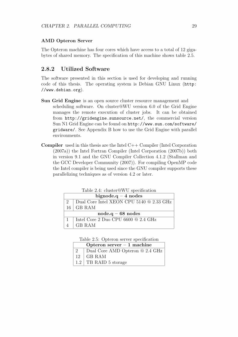
AMD Opteron Server
The Opteron machine has four cores which have access to a total of 12 giga-bytes of shared memory. The specification of this machine shows table 2.5.
2.8.2 Utilized Software
The software presented in this section is used for developing and runningcode of this thesis. The operating system is Debian GNU Linux (http://www.debian.org).
Sun Grid Engine is an open source cluster resource management andscheduling software. On cluster@WU version 6.0 of the Grid Enginemanages the remote execution of cluster jobs. It can be obtainedfrom http://gridengine.sunsource.net/, the commercial versionSun N1 Grid Engine can be found on http://www.sun.com/software/
gridware/. See Appendix B how to use the Grid Engine with parallelenvironments.
Compiler used in this thesis are the Intel C++ Compiler (Intel Corporation(2007a)) the Intel Fortran Compiler (Intel Corporation (2007b)) bothin version 9.1 and the GNU Compiler Collection 4.1.2 (Stallman andthe GCC Developer Community (2007)). For compiling OpenMP codethe Intel compiler is being used since the GNU compiler supports theseparallelizing techniques as of version 4.2 or later.
Table 2.4: cluster@WU specificationbignode.q – 4 nodes
2 Dual Core Intel XEON CPU 5140 @ 2.33 GHz16 GB RAM
node.q – 68 nodes1 Intel Core 2 Duo CPU 6600 @ 2.4 GHz4 GB RAM
Table 2.5: Opteron server specificationOpteron server – 1 machine
2 Dual Core AMD Opteron @ 2.4 GHz12 GB RAM1.2 TB RAID 5 storage

CHAPTER 2. PARALLEL COMPUTING 30
R is a free software environment for Statistical Computing and Graphics(R Development Core Team (2007b)). R-patched 2.5.1 is used in thisthesis. There is a separate chapter about R and high performancecomputing (Chapter 3).
PVM version 3.4 is used for running the corresponding programs (see Sec-tion 2.5.3).
LAM/MPI version 7.1.3 is used for running MPI programs (see Sec-tion 2.5.2).
2.9 Conclusion
This chapter provided an overview of the state of the art in parallel comput-ing. The ongoing development of computer architectures shows that paral-lel computing is becoming increasingly important as the newest commodityprocessors are already equipped with two to four computation cores. At thesame time in the high performance computing segment a further substantialincrease in parallel computational power is taken place. An interesting de-velopment certainly is grid computing. Sharing unused resources and on theother hand having access to a tremendous amount of computational powermay be the approach for large-scale computing in the future. Increasing net-work bandwidth and a growing amount of unused computational resourcesmakes this possible.
Tools for creating programs exist for every kind of platform. The mostpromising of them is certainly OpenMP which may be the paradigm of choicefor the mainstream. A lack in performance and the limitation to shared mem-ory platforms compared to message passing environments has to be consid-ered though. MPI and PVM are still commonly used as they deliver highestperformance on many different platforms through their portability. A majordisadvantage is the complexity of writing programs using message passing.Years of experience are needed to write efficient algorithms. Nevertheless, itremains to be an interesting challenge.
Chapter 3
High Performance Computingand R
3.1 Introduction
This chapter provides an overview of the capabilities of R (R DevelopmentCore Team (2007b)) in the area of high performance computing. A shortdescription of the software package R is given at the beginning of this chapter.Subsequently extensions to the base environment (so called packages) whichprovide high performance computation functionality to R are going to beexplained. Among these extensions there is the package called paRc, whichwas developed in the course of this thesis.
Examples shown in this chapter have been produced on cluster@WU (seeSection 2.8 for details).
3.2 The R Environment
R is an integrated suite of software facilities for data manipulation, calcu-lation and graphical display. R is open source originally developed by RossIhaka and Robert Gentleman (Ihaka and Gentleman (1996)). Since 1997 agroup of scientists (the “R Core Team”) is responsible for the developmentof the R-project and has write access to the source code. R has a homepagewhich can be found on http://www.R-project.org. Sources, binaries anddocumentation can be obtained from CRAN, the Comprehensive R ArchiveNetwork (http://cran.R-project.org). Among other things R has (R De-velopment Core Team (2007b))
• an effective data handling and storage facility,
31
CHAPTER 3. HIGH PERFORMANCE COMPUTING AND R 32
• a suite of operators for calculations on arrays, in particular matrices,
• a large, coherent, integrated collection of intermediate tools for dataanalysis,
• graphical facilities for data analysis and display either directly at thecomputer or on hardcopy, and
• a well developed, simple and effective programming language (called‘R’) which includes conditionals, loops, user defined recursive functionsand input and output facilities. (Indeed most of the system suppliedfunctions are themselves written in the R language.)
R is not only an environment for statistical computing and graphics butalso a freely available high-level language for programming. It can be ex-tended by standardized collections of code called “packages”. So developersand statisticians around the world can participate and provide optional codeto the base R environment. Developing and implementing new methods ofdata analysis can therefore be rather easy to achieve (for more informationabout R and on how R can be extended see Hornik (2007) and R DevelopmentCore Team (2007a)).
Now, as datasets grow bigger and bigger and algorithms become moreand more complex, R has to be made ready for high performance comput-ing. Indeed, R is already prepared through a few extensions explained inthe subsequent chapters. The packages mentioned in this chapter can beobtained from CRAN except paRc which can be obtained from R-Forge(http://R-Forge.R-project.org), a platform for collaborative software de-velopment for the R community (Theussl (2007a)).
3.3 The Rmpi Package
The Message Passing Interface (MPI) is a set of library interface standardsfor message passing and there are many implementations using these stan-dards (see also Section 2.5.2). Rmpi is an interface to MPI (Yu (2002) andYu (2006)). As of the time of this writing Rmpi uses the LAM implementa-tion of MPI. For process spawning the standard MPI-1.2 is required whichis available in the LAM/MPI implementation as LAM/MPI (version 7.1.3)supports a large portions of the MPI-2 standard. This is necessary if onelikes to use interactive spawning of R processes. With MPI versions prior toMPI-1.2 separate R processes have to be created by hand using mpirun (partof many MPI implementations) for example.
CHAPTER 3. HIGH PERFORMANCE COMPUTING AND R 33
Rmpi contains a lot of low level interface functions to the MPI C-library.Furthermore, a handful of high level functions are supplied. A selection ofroutines is going to be presented in this section.
A windows implementation of this package (which uses MPICH2) is avail-able from http://www.stats.uwo.ca/faculty/yu/Rmpi.
3.3.1 Initialization and Status Queries
The LAM/MPI environment has to be booted prior to using any messagepassing library functions. One possibility is to use the command line, theother is to load the Rmpi package. It automatically sets up a (small—1 host)LAM/MPI environment (if the executables are in the search path).
When using the Sun Grid Engine (SGE) or other queueing systems toboot the LAM/MPI parallel environment the developer is not engaged withsetting up and booting the environment anymore (see Appendix B on howto do this). On a cluster of workstations this is the method of choice.
Management and Query Functions
lamhosts() finds the hostname associated with its node number.
mpi.universe.size() returns the total number of CPUs available to theMPI environment (i.e., in a cluster or in a parallel environment startedby the grid engine).
mpi.is.master() returns TRUE if the process is the master process orFALSE otherwise.
mpi.get.processor.name() returns the hostname where the process is ex-ecuted.
mpi.finalize() cleans all MPI states (this is done when calling mpi.exit
or mpi.quit.
mpi.exit() terminates the mpi communication environment and detachesthe Rmpi package which makes reloading of the package Rmpi in thesame session impossible.
mpi.quit() terminates the mpi communication environment and quits R.
Example 3.1 shows how the configuration of the parallel environment canbe obtained. First it returns the hosts connected to the parallel environmentand then prints the number of CPUs available in it. After a query if this

CHAPTER 3. HIGH PERFORMANCE COMPUTING AND R 34
process is the master process, the hostname the current process runs on isreturned.
Example 3.1 Queries to the MPI communication environment
> library("Rmpi")> lamhosts()
node023 node023 node037 node037 node017 node017 node063 node0630 1 2 3 4 5 6 7
> mpi.universe.size()
[1] 8
> mpi.is.master()
[1] TRUE
> mpi.get.processor.name()
[1] "node023"
3.3.2 Process Spawning and Communication
In Rmpi it is easy to spawn R slaves and use them as workhorses. Thecommunication between all the involved processes is carried out in a so calledcommunicator (comm). All processes within the same communicator are ableto send or receive messages from other processes. The processes are identifiedthrough their commrank (see also the fundamentals of message passing inSection 2.5.1). The big advantage of Rmpi slaves is, that they can be usedinteractively when using the default R slave script.

CHAPTER 3. HIGH PERFORMANCE COMPUTING AND R 35
Process Management Functions
mpi.spawn.Rslaves(nslaves = mpi.universe.size(), ...) spawns anumber (nslaves) of R workhorses to those hosts automatically chosenby MPI. For other arguments represented by . . . to this function werefer to Yu (2006).
mpi.close.Rslaves(dellog = TRUE, ...) closes previously spawnedslaves and returns 1 if successful.
mpi.comm.size() returns the total number of members in a communicator.
mpi.comm.rank() returns the rank (identifier) of the process in a communi-cator.
mpi.remote.exec(cmd, ..., ret = TRUE) executes a command cmd on Rslaves with . . . arguments to cmd and returns executed results if ret
is TRUE.
In Example 3.2 as many slaves are spawned as are available in the parallelenvironment. The size of the communicator is returned (1 master plus thespawned slaves) and a remote query of the commrank is carried out. Beforethe slaves are closed the commrank of the master is printed.
Example 3.2 Process management and communication> mpi.spawn.Rslaves(nslaves = mpi.universe.size())
8 slaves are spawned successfully. 0 failed.master (rank 0, comm 1) of size 9 is running on: node023slave1 (rank 1, comm 1) of size 9 is running on: node023slave2 (rank 2, comm 1) of size 9 is running on: node023slave3 (rank 3, comm 1) of size 9 is running on: node037slave4 (rank 4, comm 1) of size 9 is running on: node037slave5 (rank 5, comm 1) of size 9 is running on: node017slave6 (rank 6, comm 1) of size 9 is running on: node017slave7 (rank 7, comm 1) of size 9 is running on: node063slave8 (rank 8, comm 1) of size 9 is running on: node063
> mpi.comm.size()[1] 9
> mpi.remote.exec(mpi.comm.rank())X1 X2 X3 X4 X5 X6 X7 X8
1 1 2 3 4 5 6 7 8
> mpi.comm.rank()[1] 0
> mpi.close.Rslaves()[1] 1

CHAPTER 3. HIGH PERFORMANCE COMPUTING AND R 36
3.3.3 Built-in High Level Functions
Rmpi provides many high level functions. We selected a few of them whichwe think are commonly used. Most of them have been utilized to buildparallel programs presented in subsequent chapters.
High Level Functions
mpi.apply(x, fun, ...) applies a function fun with additional arguments. . . to a specific part of a vector x. The return value is of type list withthe same length as of x. The length of x must not exceed the numberof R slaves spawned as each element of the vector is used exactly byone slave. To achieve some sort of load balancing one can use thecorresponding apply functions below.
mpi.applyLB(x, fun, ...) applies a function fun with additional argu-ments . . . to a specific part of a vector x. There are a few morevariants explained in Yu (2006).
mpi.bcast.cmd(cmd = NULL, rank = 0, ...) broadcasts a command cmd
from the sender rank to all R slaves and evaluates it.
mpi.bcast.Robj(obj, rank = 0, ...) broadcasts an R object obj fromprocess rank rank to all other processes (master and slaves).
mpi.bcast.Robj2slave(obj, ...) broadcasts an R object obj to all Rslaves from the master process.
mpi.parSim( ... ) carries out a Monte Carlo simulation in parallel. Fordetails on this function see the package manual (Yu (2006)) and onMonte Carlo simulation the applications in Chapter 5.
How to use the high level function mpi.apply() is shown in Example 3.3.A vector of n random numbers is generated on each of the n slaves and arereturned to the master as a list (each list element representing one row).Finally a n×n matrix is formed and printed. The output of the matrix showsfor each row the same random numbers. This is because of the fact, thateach slave has the same seed. This problem can be solved by using packageslike rsprng or rlecuyer which provide parallel random number generation(for more information see the descriptions of the packages in Section 3.7.
Example 3.3 Using mpi.apply> n <- 8> mpi.spawn.Rslaves(nslaves = n)

CHAPTER 3. HIGH PERFORMANCE COMPUTING AND R 37
8 slaves are spawned successfully. 0 failed.master (rank 0, comm 1) of size 9 is running on: node023slave1 (rank 1, comm 1) of size 9 is running on: node023slave2 (rank 2, comm 1) of size 9 is running on: node023slave3 (rank 3, comm 1) of size 9 is running on: node037slave4 (rank 4, comm 1) of size 9 is running on: node037slave5 (rank 5, comm 1) of size 9 is running on: node017slave6 (rank 6, comm 1) of size 9 is running on: node017slave7 (rank 7, comm 1) of size 9 is running on: node063slave8 (rank 8, comm 1) of size 9 is running on: node063
> x <- rep(n, n)> rows <- mpi.apply(x, runif)> X <- matrix(unlist(rows), ncol = n, byrow = TRUE)> round(X, 3)
[,1] [,2] [,3] [,4] [,5] [,6] [,7] [,8][1,] 0.621 0.209 0.038 0.319 0.595 0.437 0.034 0.344[2,] 0.621 0.209 0.038 0.319 0.595 0.437 0.034 0.344[3,] 0.621 0.209 0.038 0.319 0.595 0.437 0.034 0.344[4,] 0.621 0.209 0.038 0.319 0.595 0.437 0.034 0.344[5,] 0.621 0.209 0.038 0.319 0.595 0.437 0.034 0.344[6,] 0.621 0.209 0.038 0.319 0.595 0.437 0.034 0.344[7,] 0.621 0.209 0.038 0.319 0.595 0.437 0.034 0.344[8,] 0.621 0.209 0.038 0.319 0.595 0.437 0.034 0.344
> mpi.close.Rslaves()
[1] 1
3.3.4 Other Important Functions
To complete the set of important functions supplied by the Rmpi packagethe following functions have to be explained.
Collective Communication Routines
.mpi.gather(x, type, rdata, root = 0, ...) gathers data distr-ibuted on the nodes (x) to a specific process (mostly the master) intoa single array or list (depending on the length of the data) of typetype which can be integer, double or character. It performs a sendof messages from each member in a communicator. A specific process(root) accumulates this messages into a single array or list preparedwith the rdata command.

CHAPTER 3. HIGH PERFORMANCE COMPUTING AND R 38
.mpi.scatter(x, type, rdata, root = 0, ...) sends to each memberof a communicator a partition of a vector x, type type which can beinteger, double or character, from a specified member of the group(mostly the master). Each member of the communicator receive itspart of x after preparing the receive buffer with the argument rdata.
3.3.5 Conclusion
The package Rmpi implements many of the routines available in MPI-2.But there are routines that have to be omitted or are not included becausethey are not needed for use with R (e.g., data management routines are notnecessary as R has its own tools for data handling). A really interestingaspect of the Rmpi package is the possibility to spawn interactive R slaves.That enables the user to interactively define functions which can be executedremotely on the slaves in parallel. An example how one can do this is shownin Chapter 4, where the implementation of matrix multiplication is shown. Amajor disadvantage is that MPI in its current implementations lacks in faulttolerance. This results in a rather instable execution of MPI applications.Moreover, debugging is really difficult as there is no support for it in Rmpi.
All in all this package is a good start in creating parallel programs as thiscan easy be achieved entirely in R.
For further interface functions supplied by the Rmpi package, a more de-tailed description and further examples please consult the package descriptionYu (2006).
3.4 The rpvm Package
Parallel virtual machine uses the message passing model and makes a collec-tion of computers appear as a single virtual machine (see Section 2.5.3 fordetails). The package rpvm (Li and Rossini. (2007)) provides an interface tolow level PVM functions and a few high level parallel functions to R. It usesmost of the facilities provided by the PVM system which makes rpvm idealfor prototyping parallel statistical applications in R.
Generally, parallel applications can be either written in compiled lan-guages like C or FORTRAN or can be called as R processes. The lattermethod is used in this thesis and therefore a good selection of rpvm func-tions are explained in this section to show how PVM and R can be usedtogether.
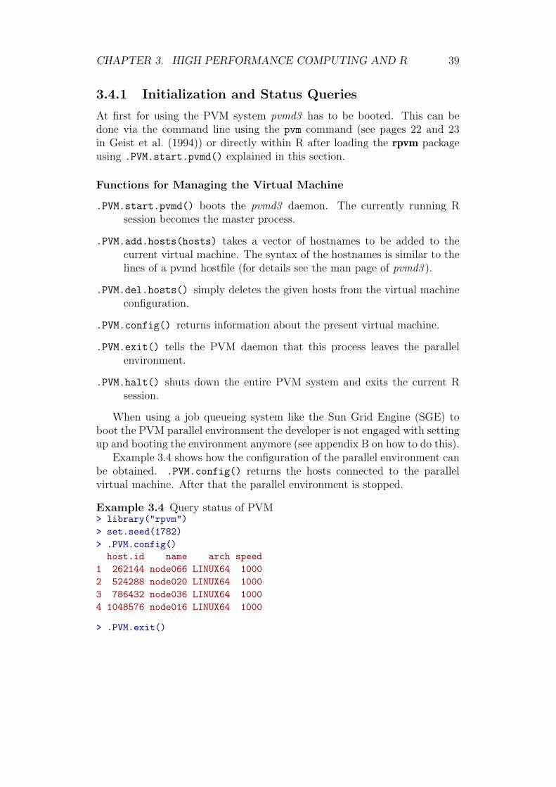
CHAPTER 3. HIGH PERFORMANCE COMPUTING AND R 39
3.4.1 Initialization and Status Queries
At first for using the PVM system pvmd3 has to be booted. This can bedone via the command line using the pvm command (see pages 22 and 23in Geist et al. (1994)) or directly within R after loading the rpvm packageusing .PVM.start.pvmd() explained in this section.
Functions for Managing the Virtual Machine
.PVM.start.pvmd() boots the pvmd3 daemon. The currently running Rsession becomes the master process.
.PVM.add.hosts(hosts) takes a vector of hostnames to be added to thecurrent virtual machine. The syntax of the hostnames is similar to thelines of a pvmd hostfile (for details see the man page of pvmd3 ).
.PVM.del.hosts() simply deletes the given hosts from the virtual machineconfiguration.
.PVM.config() returns information about the present virtual machine.
.PVM.exit() tells the PVM daemon that this process leaves the parallelenvironment.
.PVM.halt() shuts down the entire PVM system and exits the current Rsession.
When using a job queueing system like the Sun Grid Engine (SGE) toboot the PVM parallel environment the developer is not engaged with settingup and booting the environment anymore (see appendix B on how to do this).
Example 3.4 shows how the configuration of the parallel environment canbe obtained. .PVM.config() returns the hosts connected to the parallelvirtual machine. After that the parallel environment is stopped.
Example 3.4 Query status of PVM> library("rpvm")> set.seed(1782)> .PVM.config()host.id name arch speed
1 262144 node066 LINUX64 10002 524288 node020 LINUX64 10003 786432 node036 LINUX64 10004 1048576 node016 LINUX64 1000
> .PVM.exit()
CHAPTER 3. HIGH PERFORMANCE COMPUTING AND R 40
3.4.2 Process Spawning and Communication
The package rpvm uses the master-slave paradigm meaning that one processis the master task and the others are slave tasks. rpvm provides a routineto spawn R slaves but these slaves cannot be used interactively like theslaves in Rmpi. The spawned R slaves source an R script which containsall the necessary function calls to set up communication and carry out thecomputation and after processing terminate. PVM uses task IDs (tid—apositive integer for identifying a task) and tags for communication (see alsothe fundamentals of message passing in Section 2.5.1).
Process Management Functions
.PVM.spawnR(slave, ntask = 1, ...) spawns ntask copies of an slave
R process. slave is a character specifying the source file for the Rslaves located in the package’s demo directory (the default). Thereare more parameters indicated by the . . . (we refer to Li and Rossini.(2007)). The tids of the successfully spawned R slaves are returned.
.PVM.mytid() returns the tid of the calling process.
.PVM.parent() returns the tid of the parent process that spawned the call-ing process.
.PVM.siblings() returns the tid of the processes that were spawned in asingle spawn call.
.PVM.pstats(tids) returns the status of the PVM process(es) with taskID(s) tids.
3.4.3 Built-in High Level Functions
rpvm provides only two high level functions. One of them is a function toget or set values in the virtual machine settings. This is certainly becauseeach new high level functions needs separate source files for the slaves andthis is not what developers do intuitively.
High Level Functions
PVM.rapply(X, FUN = mean, NTASK = 1)) Apply a function FUN to therows of a matrix X in parallel using NTASK tasks.
PVM.options(option, value) Get or set values of libpvm options (for de-tails see Li and Rossini. (2007) and Geist et al. (1994)).

CHAPTER 3. HIGH PERFORMANCE COMPUTING AND R 41
Example 3.5 shows how the rows of a matrix X can be summed up inparallel via PVM.rapply().
Example 3.5 Using PVM.rapply
> n <- 8> X <- matrix(rnorm(n * n), nrow = n)> round(X, 3)
[,1] [,2] [,3] [,4] [,5] [,6] [,7] [,8][1,] -0.200 -0.183 0.560 1.286 0.468 0.502 0.874 -0.778[2,] -1.371 0.484 -0.498 1.788 0.534 -0.566 0.152 -1.307[3,] 1.041 0.484 0.399 0.580 0.586 -0.660 1.833 -1.405[4,] -1.117 -0.893 0.408 -1.612 0.486 0.644 0.422 -1.639[5,] 1.397 -0.237 -1.287 -0.122 -1.076 0.225 -0.047 0.020[6,] -0.046 0.537 -1.287 -0.089 0.564 2.671 -0.715 -0.901[7,] 1.085 0.706 -0.034 0.929 0.057 -2.402 -1.233 1.135[8,] 0.605 -0.076 -0.554 1.385 -0.436 0.249 0.338 1.369
> PVM.rapply(X, sum, 3)
Try to spawn tasks...Work sent to 524289Work sent to 786433Work sent to 1048577[1] 2.5291297 -0.7840539 2.8572559 -3.3002539 -1.1275728[6] 0.7329710 0.2431164 2.8806456
Before we explain how PVM.rapply works the following rpvm functionshave to be explained:
Other Important functions
.PVM.initsend() clears the default send buffer and prepares it for packinga new message.
.PVM.pkstr(data = "") and .PVM.pkint(data = 0, stride = 1) are lowlevel correspondents of the PVM packing routines (see Geist et al.(1994) for more information on packing data).
.PVM.pkdblmat(data) packs a double matrix including the dimension infor-mation. There are more packing routines available. They are explainedin Li and Rossini. (2007).
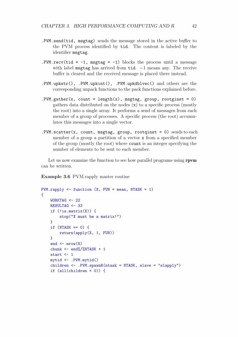
CHAPTER 3. HIGH PERFORMANCE COMPUTING AND R 42
.PVM.send(tid, msgtag) sends the message stored in the active buffer tothe PVM process identified by tid. The content is labeled by theidentifier msgtag.
.PVM.recv(tid = -1, msgtag = -1) blocks the process until a messagewith label msgtag has arrived from tid. −1 means any. The receivebuffer is cleared and the received message is placed there instead.
.PVM.upkstr(), .PVM.upkint(), .PVM.upkdblvec() and others are thecorresponding unpack functions to the pack functions explained before.
.PVM.gather(x, count = length(x), msgtag, group, rootginst = 0)
gathers data distributed on the nodes (x) to a specific process (mostlythe root) into a single array. It performs a send of messages from eachmember of a group of processes. A specific process (the root) accumu-lates this messages into a single vector.
.PVM.scatter(x, count, msgtag, group, rootqinst = 0) sends to eachmember of a group a partition of a vector x from a specified memberof the group (mostly the root) where count is an integer specifying thenumber of elements to be sent to each member.
Let us now examine the function to see how parallel programs using rpvmcan be written.
Example 3.6 PVM.rapply master routine
PVM.rapply <- function (X, FUN = mean, NTASK = 1){
WORKTAG <- 22RESULTAG <- 33if (!is.matrix(X)) {
stop("X must be a matrix!")}if (NTASK == 0) {
return(apply(X, 1, FUN))}end <- nrow(X)chunk <- end%/%NTASK + 1start <- 1mytid <- .PVM.mytid()children <- .PVM.spawnR(ntask = NTASK, slave = "slapply")if (all(children < 0)) {

CHAPTER 3. HIGH PERFORMANCE COMPUTING AND R 43
cat("Failed to spawn any task: ", children, "\n").PVM.exit()
}else if (any(children < 0)) {
cat("Failed to spawn some tasks. Successfully spawned ",sum(children > 0), "tasks\n")
children <- children[children > 0]}for (id in 1:length(children)) {
.PVM.initsend()range <- c(start, ifelse((start + chunk - 1) > end, end,
start + chunk - 1))work <- X[(range[1]):(range[2]), , drop = FALSE]start <- start + chunk.PVM.pkstr(deparse(substitute(FUN))).PVM.pkint(id).PVM.pkdblmat(work).PVM.send(children[id], WORKTAG)cat("Work sent to ", children[id], "\n")
}partial.results <- list()for (child in children) {
.PVM.recv(-1, RESULTAG)order <- .PVM.upkint()partial.results[[order]] <- .PVM.upkdblvec()
}.PVM.exit()return(unlist(partial.results))
}
The corresponding slave R script (slapply.R) looks as follows:
Example 3.7 PVM.rapply slave routine
library (rpvm)WORKTAG <- 22RESULTAG <- 33mytid <- .PVM.mytid ()myparent <- .PVM.parent ()## Receive work from parent (a matrix)buf <- .PVM.recv (myparent, WORKTAG)## Function to applyfunc <- .PVM.upkstr ()

CHAPTER 3. HIGH PERFORMANCE COMPUTING AND R 44
cat ("Function to apply: ", func, "\n")## Orderorder <- .PVM.upkint ()partial.work <- .PVM.upkdblmat ()print (partial.work)## actually work, take the mean of the rowspartial.result <- apply (partial.work, 1, func)print (partial.result)## Send result back.PVM.initsend ().PVM.pkint (order).PVM.pkdblvec (partial.result).PVM.send (myparent, RESULTAG)## Exit PVM.PVM.exit ()## Exit Rq (save="no")
Example 3.6 shows the master routine of PVM.rapply(). This functiontakes a matrix, the function which is going to be applied and the numberof processors to use as arguments. At first the message tags are specified.These tags are necessary to uniquely identify messages sent in a message pass-ing environment. After input validation NTASK child processes are spawnedusing the .PVM.spawnR() command. After initializing the send buffer thepartitioned data (packed in the buffer using the .PVM.pk* commands) issend to the corresponding child processes represented by their task IDs using.PVM.send(). PVM uses these task identifiers (tid) to address pvmds, tasks,and groups of tasks within a virtual machine.
Meanwhile the spawned slave processes (see Example 3.7) have been idlebecause they wait for input (.PVM.receive() is a blocking command). Afterreceiving data from the parent the data gets unpacked. Now the slavesapply the given function to their part of the matrix. Finally another sendis initialized to provide the results to the parent process and the slaves aredetached from the virtual machine by calling a .PVM.exit().
3.4.4 Conclusion
The PVM.rapply() example shown in this section followed the Single Pro-gram Multiple Data (SPMD) paradigm. Data is split into different partswhich are sent to different processes. I/O is handled solely by a master pro-cess. When loading rpvm in an R session this session becomes the master
CHAPTER 3. HIGH PERFORMANCE COMPUTING AND R 45
process. Slaves can easily be spawned provided that there are working slavescripts available.
We encountered no problems when using the routines in rpvm. Thispackage seem to be rather stable in contrast to Rmpi, where for unknownreasons the MPI environment sometimes crashed.
A major disadvantage is that the rpvm package only has two higher levelfunction. One of them can be used for calculations. That means whenusing this package for parallel computing one has to deal with low level mes-sage passing but which in turn may provide higher flexibility. New parallelfunctions can be constructed on the basis of the provided interface. ThePVM.rapply code can be taken as a template for further routines.
Another disadvantage is the missing support for interactive R slaves. Par-allel tasks have to be created on the basis of separate slave source files whichare sourced on the creation of the slaves.
For further interface functions supplied by the rpvm package, a more de-tailed description and further examples please consult the package descriptionLi and Rossini. (2007).
3.5 The snow Package
The aim of simple network of workstations (snow—Rossini et al. (2003),Tierney et al. (2007)) is to provide a simple parallel computing environmentin R. To make a collection of computers to appear as a virtual cluster in Rthree different message passing environments can be used:
• PVM via R package rpvm (see section 3.4)
• MPI via R package Rmpi (see section 3.3)
• SOCK via TCP sockets
The details of the mechanism used and how it implemented are hiddenfrom the high level user. As the name suggests it should be simple to use.
After setting up a virtual cluster developing parallel R functions can beachieved via a standardized interface to the computation nodes.
Moreover, when using snow one can rely on a good handful of high levelfunctions. This makes it rather easy to use the underlying parallel computa-tional engine. Indeed snow uses existing interfaces to R namely Rmpi whenusing MPI (see Section 3.3), rpvm when using PVM (see Section 3.4) anda new possibility of message passing namely TCP sockets, which is a rathersimple way of achieving communication between nodes (in most applications
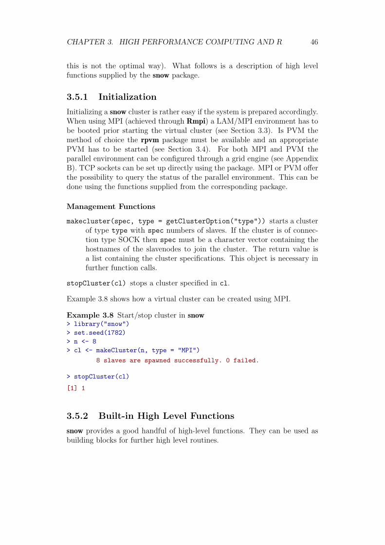
CHAPTER 3. HIGH PERFORMANCE COMPUTING AND R 46
this is not the optimal way). What follows is a description of high levelfunctions supplied by the snow package.
3.5.1 Initialization
Initializing a snow cluster is rather easy if the system is prepared accordingly.When using MPI (achieved through Rmpi) a LAM/MPI environment has tobe booted prior starting the virtual cluster (see Section 3.3). Is PVM themethod of choice the rpvm package must be available and an appropriatePVM has to be started (see Section 3.4). For both MPI and PVM theparallel environment can be configured through a grid engine (see AppendixB). TCP sockets can be set up directly using the package. MPI or PVM offerthe possibility to query the status of the parallel environment. This can bedone using the functions supplied from the corresponding package.
Management Functions
makecluster(spec, type = getClusterOption("type")) starts a clusterof type type with spec numbers of slaves. If the cluster is of connec-tion type SOCK then spec must be a character vector containing thehostnames of the slavenodes to join the cluster. The return value isa list containing the cluster specifications. This object is necessary infurther function calls.
stopCluster(cl) stops a cluster specified in cl.
Example 3.8 shows how a virtual cluster can be created using MPI.
Example 3.8 Start/stop cluster in snow> library("snow")> set.seed(1782)> n <- 8> cl <- makeCluster(n, type = "MPI")
8 slaves are spawned successfully. 0 failed.
> stopCluster(cl)
[1] 1
3.5.2 Built-in High Level Functions
snow provides a good handful of high-level functions. They can be used asbuilding blocks for further high level routines.

CHAPTER 3. HIGH PERFORMANCE COMPUTING AND R 47
High Level Functions
clusterEvalQ(cl, expr) evaluates an R expression expr on each clusternode provided by cl.
clusterCall(cl, fun, ...) calls a function fun with arguments . . . oneach node found in cl and returns a list of the results.
clusterApply(cl, x, fun, ...) applies a function fun with additionalarguments . . . to a specific part of a vector x. The return value is oftype list with the same length as of x. The length of x must not exceedthe number of R slaves spawned as each element of the vector is usedexactly by one slave. To achieve some sort of load balancing please usethe corresponding apply functions below.
clusterApplyLB(cl, x, fun, ...) is a load balancing version ofclusterApply() which applies a function fun with additional argu-ments . . . to a specific part of a vector x with the difference that thelength of x can exceed the number of cluster nodes. If a node finishedwith the computation the next job is placed on the available node. Thisis repeated until all jobs have completed.
clusterExport(cl, list) broadcasts a list of global variables on the mas-ter (list) to all slaves.
parApply(cl, x, fun, ...) is one of the parallel versions of the apply
functions available in R. We refer to the package documentation (Tier-ney et al. (2007)) for further details.
parMM(cl, A,B) is a simple parallel implementation of matrix multiplica-tion.
Example 3.9 shows the use of clusterApply() on a virtual cluster of 8nodes using MPI as communication layer. Like in Example 3.3 a vector ofn random numbers is generated on each of the n slaves and are returnedto the master as a list (each list element representing one row). Finally ann × n matrix is formed and printed. The output of the matrix shows againfor each row the same random numbers. This is because of the fact, thateach slave has the same seed. This problem is treated more specifically inChapter 5. For more information about parallel random number generatorssee the descriptions of the packages rsprng and rlecuyer in Section 3.7.
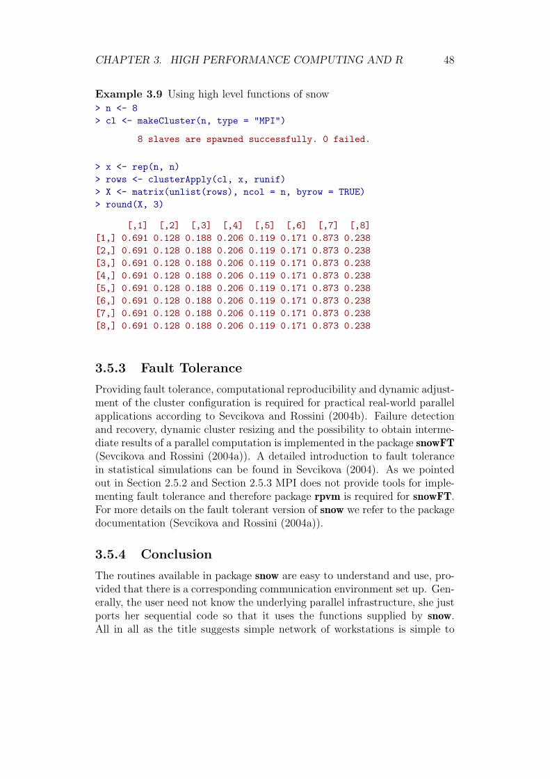
CHAPTER 3. HIGH PERFORMANCE COMPUTING AND R 48
Example 3.9 Using high level functions of snow> n <- 8> cl <- makeCluster(n, type = "MPI")
8 slaves are spawned successfully. 0 failed.
> x <- rep(n, n)> rows <- clusterApply(cl, x, runif)> X <- matrix(unlist(rows), ncol = n, byrow = TRUE)> round(X, 3)
[,1] [,2] [,3] [,4] [,5] [,6] [,7] [,8][1,] 0.691 0.128 0.188 0.206 0.119 0.171 0.873 0.238[2,] 0.691 0.128 0.188 0.206 0.119 0.171 0.873 0.238[3,] 0.691 0.128 0.188 0.206 0.119 0.171 0.873 0.238[4,] 0.691 0.128 0.188 0.206 0.119 0.171 0.873 0.238[5,] 0.691 0.128 0.188 0.206 0.119 0.171 0.873 0.238[6,] 0.691 0.128 0.188 0.206 0.119 0.171 0.873 0.238[7,] 0.691 0.128 0.188 0.206 0.119 0.171 0.873 0.238[8,] 0.691 0.128 0.188 0.206 0.119 0.171 0.873 0.238
3.5.3 Fault Tolerance
Providing fault tolerance, computational reproducibility and dynamic adjust-ment of the cluster configuration is required for practical real-world parallelapplications according to Sevcikova and Rossini (2004b). Failure detectionand recovery, dynamic cluster resizing and the possibility to obtain interme-diate results of a parallel computation is implemented in the package snowFT(Sevcikova and Rossini (2004a)). A detailed introduction to fault tolerancein statistical simulations can be found in Sevcikova (2004). As we pointedout in Section 2.5.2 and Section 2.5.3 MPI does not provide tools for imple-menting fault tolerance and therefore package rpvm is required for snowFT.For more details on the fault tolerant version of snow we refer to the packagedocumentation (Sevcikova and Rossini (2004a)).
3.5.4 Conclusion
The routines available in package snow are easy to understand and use, pro-vided that there is a corresponding communication environment set up. Gen-erally, the user need not know the underlying parallel infrastructure, she justports her sequential code so that it uses the functions supplied by snow.All in all as the title suggests simple network of workstations is simple to
CHAPTER 3. HIGH PERFORMANCE COMPUTING AND R 49
get started with and is simple with respect to the possibilities of parallelcomputations.
For further interface functions supplied by the snow package, a more de-tailed description and further examples please consult the package descriptionTierney et al. (2007).
3.6 paRc—PARallel Computations in R
In the course of this thesis a package called paRc (Theussl (2007b)) has beendeveloped with the aim to evaluate performance of parallel applications andto show how interfacing high performance applications written in C can bedone using OpenMP (see Section 2.5.4).
The package paRc contains interface functions to the OpenMP libraryand provides high level interface functions to a few C implementations ofparallel applications using OpenMP (e.g., matrix multiplication—see Chap-ter 4). Furthermore, it supplies a benchmark environment for performanceevaluation of parallel programs and a framework for pricing options withparallel Monte Carlo simulation (see Chapter 5).
paRc can be obtained from R-Forge.R-project.org—the R-project com-munity service. To install this package directly within R callinstall.packages("paRc", repos = "R-Forge.R-project.org").
To properly install this package you need either the Intel compiler withversion 9.1 or newer (the Linux compiler is free for non-commercial use) orthe GNU C compiler with version 4.2 or newer. They are known to supportOpenMP.
Examples in this section are produced on a bignode of cluster@WU. Big-nodes provide a shared memory platform with up to 4 CPUs. Shared memoryplatforms are necessary for running parallel OpenMP applications.
3.6.1 OpenMP Interface Functions
The user is provided with a few interface functions to the OpenMP library.They are used to query the internal variables of the compiled parallel envi-ronment or to change them.
OpenMP Routines
omp get num procs() returns the number of threads available to the pro-gram.
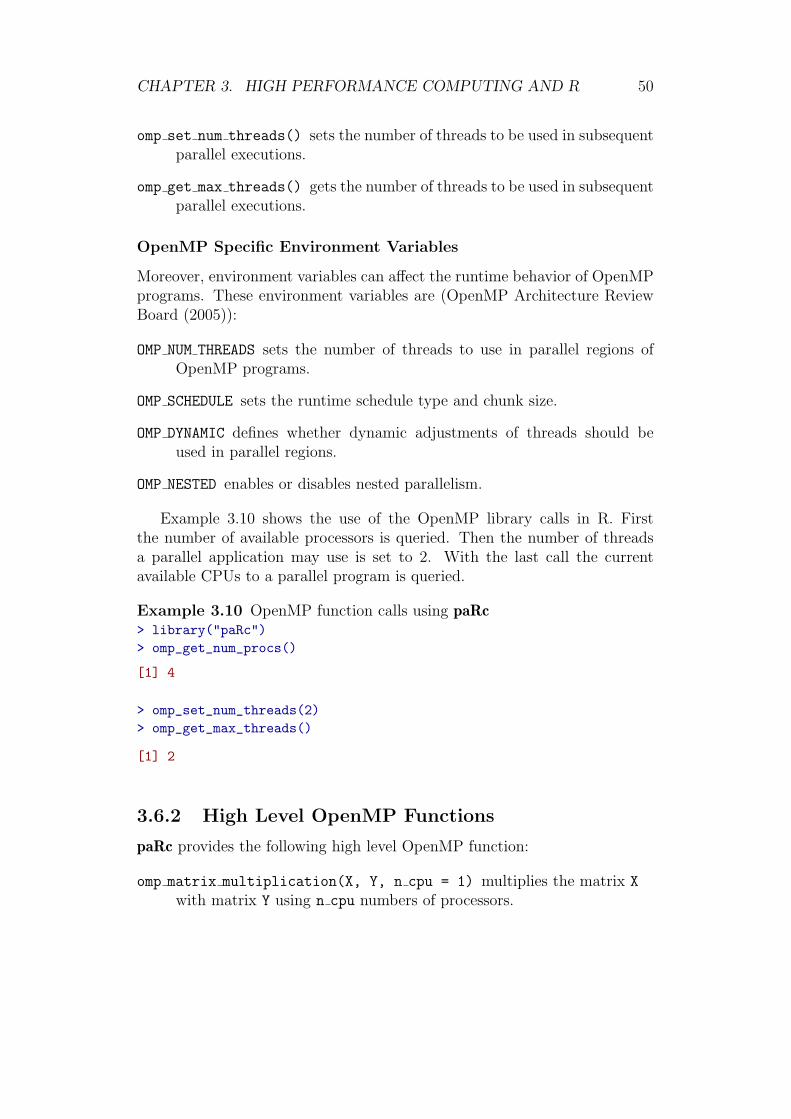
CHAPTER 3. HIGH PERFORMANCE COMPUTING AND R 50
omp set num threads() sets the number of threads to be used in subsequentparallel executions.
omp get max threads() gets the number of threads to be used in subsequentparallel executions.
OpenMP Specific Environment Variables
Moreover, environment variables can affect the runtime behavior of OpenMPprograms. These environment variables are (OpenMP Architecture ReviewBoard (2005)):
OMP NUM THREADS sets the number of threads to use in parallel regions ofOpenMP programs.
OMP SCHEDULE sets the runtime schedule type and chunk size.
OMP DYNAMIC defines whether dynamic adjustments of threads should beused in parallel regions.
OMP NESTED enables or disables nested parallelism.
Example 3.10 shows the use of the OpenMP library calls in R. Firstthe number of available processors is queried. Then the number of threadsa parallel application may use is set to 2. With the last call the currentavailable CPUs to a parallel program is queried.
Example 3.10 OpenMP function calls using paRc> library("paRc")> omp_get_num_procs()
[1] 4
> omp_set_num_threads(2)> omp_get_max_threads()
[1] 2
3.6.2 High Level OpenMP Functions
paRc provides the following high level OpenMP function:
omp matrix multiplication(X, Y, n cpu = 1) multiplies the matrix X
with matrix Y using n cpu numbers of processors.

CHAPTER 3. HIGH PERFORMANCE COMPUTING AND R 51
3.6.3 Benchmark Environment
paRc provides a benchmark environment for measuring the performance ofparallel programs. Two main functions exist in this context—one for creatinga benchmark object and one for running the benchmark described by theobject.
Class ‘benchmark’
An S3 object (Chambers and Hastie (1991)) of class ‘benchmark’ contains allthe necessary information to run a benchmark. The elements in the objectare
task is a character string defining the task of the benchmark. Currently, thefollowing tasks are implemented:
• matrix multiplication
• Monte Carlo simulation
data is a list containing the parameters and data to properly run the task.
type defines the parallel programming model used to run the benchmark.Currently, the following types are implemented (not necessarily all ofthem are available for each task):
• OpenMP—C interface calls provided by paRc,
• MPI—implementation in paRc using Rmpi for communication,
• PVM—implementation in paRc using rpvm for communication,
• snow-MPI—implementation in snow using Rmpi for communica-tion,
• and snow-PVM—implementation in snow using rpvm for commu-nication.
cpu range contains a vector of integers representing the number of CPUsfor th corresponding benchmark run.
is parallel is a logical TRUE or FALSE whether the benchmark contains par-allel tasks or not.
runs is an integer defining the number of repetitions of the benchmark.
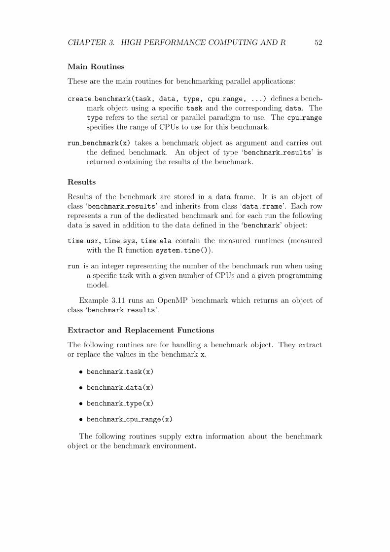
CHAPTER 3. HIGH PERFORMANCE COMPUTING AND R 52
Main Routines
These are the main routines for benchmarking parallel applications:
create benchmark(task, data, type, cpu range, ...) defines a bench-mark object using a specific task and the corresponding data. Thetype refers to the serial or parallel paradigm to use. The cpu range
specifies the range of CPUs to use for this benchmark.
run benchmark(x) takes a benchmark object as argument and carries outthe defined benchmark. An object of type ‘benchmark results’ isreturned containing the results of the benchmark.
Results
Results of the benchmark are stored in a data frame. It is an object ofclass ‘benchmark results’ and inherits from class ‘data.frame’. Each rowrepresents a run of the dedicated benchmark and for each run the followingdata is saved in addition to the data defined in the ‘benchmark’ object:
time usr, time sys, time ela contain the measured runtimes (measuredwith the R function system.time()).
run is an integer representing the number of the benchmark run when usinga specific task with a given number of CPUs and a given programmingmodel.
Example 3.11 runs an OpenMP benchmark which returns an object ofclass ‘benchmark results’.
Extractor and Replacement Functions
The following routines are for handling a benchmark object. They extractor replace the values in the benchmark x.
• benchmark task(x)
• benchmark data(x)
• benchmark type(x)
• benchmark cpu range(x)
The following routines supply extra information about the benchmarkobject or the benchmark environment.

CHAPTER 3. HIGH PERFORMANCE COMPUTING AND R 53
benchmark is parallel returns TRUE if the benchmark contains a parallelfunction to apply.
benchmark tasks returns the tasks which are possible to run with the bench-mark environment.
benchmark types returns the types of available serial or parallel paradigmsto run with the benchmark environment.
Generic Functions
Generic functions provide methods for different objects. In paRc a genericfunction for calculating the speedup is provided:
speedup(x) is a generic function taking an object as an argument. Cur-rently there are two methods implemented namely speedup.numeric
and speedup.benchmark results. The methods calculate the speedupas it is presented in Equation 2.1.
S3 Methods
The following S3 methods are provided for the benchmark environment:
print.benchmark prints objects of class ‘benchmark’
plot.benchmark results supplies a plot method for comparing benchmarkresults.
speedup.default returns an error message that there is no default method.
speedup.numeric returns the speedups calculated from a vector of type‘numeric’. The reference execution time is the first element in thevector. The return value is a vector of type ‘numeric’.
speedup.benchmark results calculates the speedups from a given object ofclass ‘benchmark results’ and the results are returned as a vector oftype ‘numeric’.
Example 3.11 Running a benchmark using OpenMP
> n <- 1000> max_cpu <- omp_get_num_procs()> dat <- list()> dat[[1]] <- dat[[2]] <- n> dat[[3]] <- function(x) {
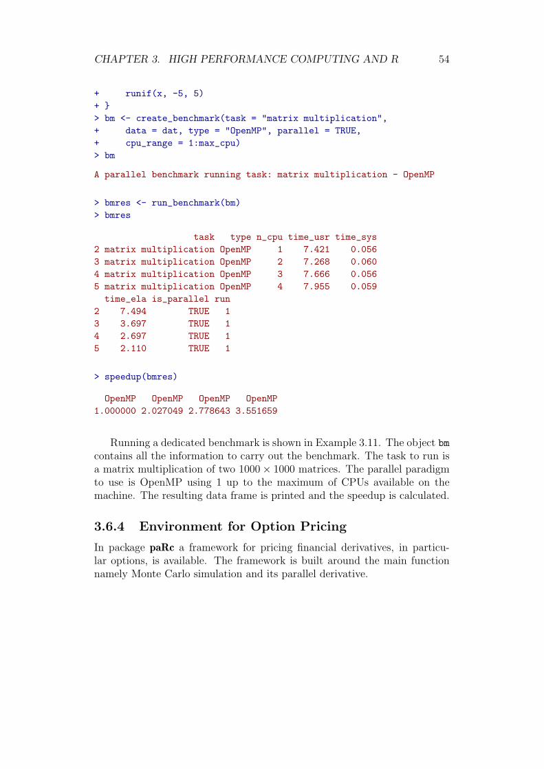
CHAPTER 3. HIGH PERFORMANCE COMPUTING AND R 54
+ runif(x, -5, 5)+ }> bm <- create_benchmark(task = "matrix multiplication",+ data = dat, type = "OpenMP", parallel = TRUE,+ cpu_range = 1:max_cpu)> bm
A parallel benchmark running task: matrix multiplication - OpenMP
> bmres <- run_benchmark(bm)> bmres
task type n_cpu time_usr time_sys2 matrix multiplication OpenMP 1 7.421 0.0563 matrix multiplication OpenMP 2 7.268 0.0604 matrix multiplication OpenMP 3 7.666 0.0565 matrix multiplication OpenMP 4 7.955 0.059
time_ela is_parallel run2 7.494 TRUE 13 3.697 TRUE 14 2.697 TRUE 15 2.110 TRUE 1
> speedup(bmres)
OpenMP OpenMP OpenMP OpenMP1.000000 2.027049 2.778643 3.551659
Running a dedicated benchmark is shown in Example 3.11. The object bmcontains all the information to carry out the benchmark. The task to run isa matrix multiplication of two 1000× 1000 matrices. The parallel paradigmto use is OpenMP using 1 up to the maximum of CPUs available on themachine. The resulting data frame is printed and the speedup is calculated.
3.6.4 Environment for Option Pricing
In package paRc a framework for pricing financial derivatives, in particu-lar options, is available. The framework is built around the main functionnamely Monte Carlo simulation and its parallel derivative.
CHAPTER 3. HIGH PERFORMANCE COMPUTING AND R 55
Class ‘option’
An S3 object of class ‘option’ contains all the necessary information forpricing an option. The list elements are
underlying is a numeric vector containing three elements to describe astock:
• the return µ,
• the volatility σ,
• and the present value of the stock.
strike price is a numeric defining the strike price of the option.
maturity is a numeric defining the time until the option expires.
type is a character representing the type of the option. There are twopossibilities—either a "Call" option, or a "Put" option.
kind contains a character representing the class of the option. Only optionsof type "European" can be priced at the time of this writing.
position is a character string marking the position of the investor. This caneither be "long" or "short".
Main Routines
These are the main routines for pricing an option:
define option(underlying, strike price, maturity, ...) defines anobject of class ‘option’. Further arguments represented by the . . . aretype (with default "Call"), class (default "European") and position
(default "long").
Black Scholes price(x) takes an object of class ‘option’ as argument andreturns the analytical solution of the Black Scholes differential equation(the price of the option). This works only for European options (seeSection 5.2.2 for details).
Monte Carlo simulation(x, r, path length, n paths, ...) carries outa Monte Carlo simulation pricing an option given by x. Further argu-ments are the risk free yield r, the length of a Wiener path path length,the number of simulated paths n paths, the number of simulation runsn simulations (with default 50) and if antithetic variance reductionshould be used (antithetic = TRUE).
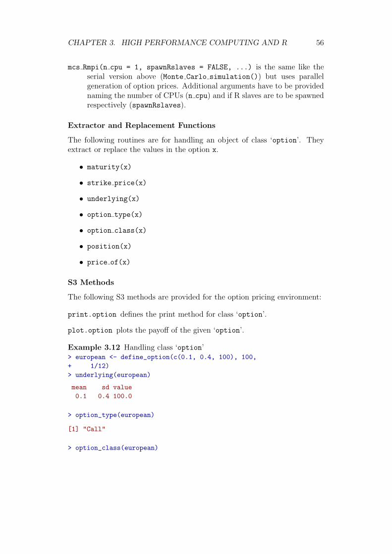
CHAPTER 3. HIGH PERFORMANCE COMPUTING AND R 56
mcs Rmpi(n cpu = 1, spawnRslaves = FALSE, ...) is the same like theserial version above (Monte Carlo simulation()) but uses parallelgeneration of option prices. Additional arguments have to be providednaming the number of CPUs (n cpu) and if R slaves are to be spawnedrespectively (spawnRslaves).
Extractor and Replacement Functions
The following routines are for handling an object of class ‘option’. Theyextract or replace the values in the option x.
• maturity(x)
• strike price(x)
• underlying(x)
• option type(x)
• option class(x)
• position(x)
• price of(x)
S3 Methods
The following S3 methods are provided for the option pricing environment:
print.option defines the print method for class ‘option’.
plot.option plots the payoff of the given ‘option’.
Example 3.12 Handling class ‘option’> european <- define_option(c(0.1, 0.4, 100), 100,+ 1/12)> underlying(european)
mean sd value0.1 0.4 100.0
> option_type(european)
[1] "Call"
> option_class(european)
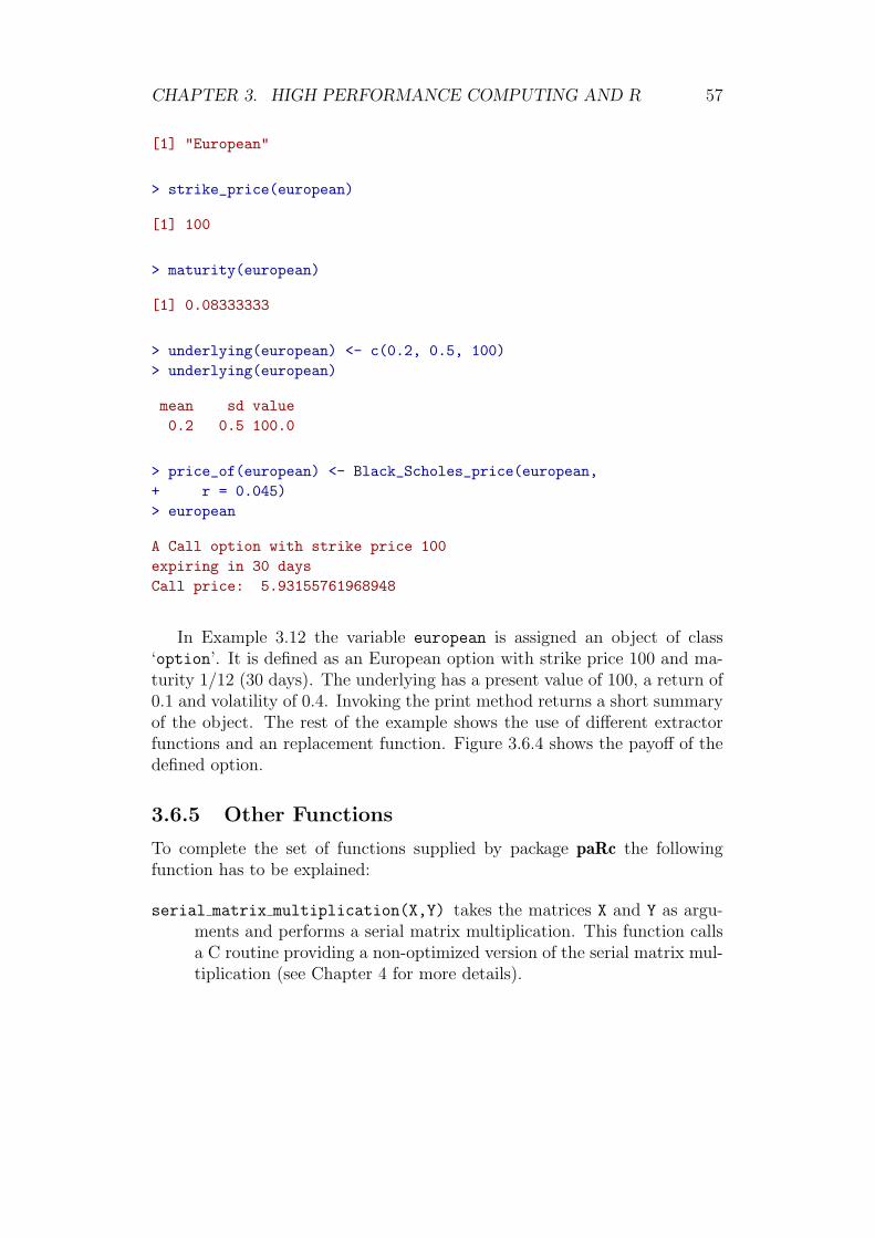
CHAPTER 3. HIGH PERFORMANCE COMPUTING AND R 57
[1] "European"
> strike_price(european)
[1] 100
> maturity(european)
[1] 0.08333333
> underlying(european) <- c(0.2, 0.5, 100)> underlying(european)
mean sd value0.2 0.5 100.0
> price_of(european) <- Black_Scholes_price(european,+ r = 0.045)> european
A Call option with strike price 100expiring in 30 daysCall price: 5.93155761968948
In Example 3.12 the variable european is assigned an object of class‘option’. It is defined as an European option with strike price 100 and ma-turity 1/12 (30 days). The underlying has a present value of 100, a return of0.1 and volatility of 0.4. Invoking the print method returns a short summaryof the object. The rest of the example shows the use of different extractorfunctions and an replacement function. Figure 3.6.4 shows the payoff of thedefined option.
3.6.5 Other Functions
To complete the set of functions supplied by package paRc the followingfunction has to be explained:
serial matrix multiplication(X,Y) takes the matrices X and Y as argu-ments and performs a serial matrix multiplication. This function callsa C routine providing a non-optimized version of the serial matrix mul-tiplication (see Chapter 4 for more details).
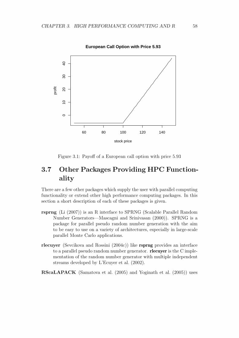
CHAPTER 3. HIGH PERFORMANCE COMPUTING AND R 58
60 80 100 120 140
010
2030
40
European Call Option with Price 5.93
stock price
prof
it
Figure 3.1: Payoff of a European call option with price 5.93
3.7 Other Packages Providing HPC Function-
ality
There are a few other packages which supply the user with parallel computingfunctionality or extend other high performance computing packages. In thissection a short description of each of these packages is given.
rsprng (Li (2007)) is an R interface to SPRNG (Scalable Parallel RandomNumber Generators—Mascagni and Srinivasan (2000)). SPRNG is apackage for parallel pseudo random number generation with the aimto be easy to use on a variety of architectures, especially in large-scaleparallel Monte Carlo applications.
rlecuyer (Sevcikova and Rossini (2004c)) like rsprng provides an interfaceto a parallel pseudo random number generator. rlecuyer is the C imple-mentation of the random number generator with multiple independentstreams developed by L’Ecuyer et al. (2002).
RScaLAPACK (Samatova et al. (2005) and Yoginath et al. (2005)) uses

CHAPTER 3. HIGH PERFORMANCE COMPUTING AND R 59
the high performance ScaLAPACK library (Dongarra et al. (1997))forlinear algebra computations. ScaLAPACK is a library of high perfor-mance linear algebra routines which makes use of message passing torun on distributed memory machines. Among other routines it providesfunctionality to solve systems of linear equations, linear least squaresproblems, eigenvalue problems and singular value problems. ScaLA-PACK is an acronym for Scalable Linear Algebra PACKage or ScalableLAPACK. Samatova et al. (2006) have shown how to use RScaLA-PACK in biology and climate modelling and analyzed its performance.
papply (Currie (2005)) implements a similar interface to lapply and applybut distributes the processing evenly among the nodes of a cluster.papply uses the package Rmpi (see Section 3.3) for communication butsupports in addition error messages for debugging.
biopara (Lazar and Schoenfeld (2006)) allows users to distribute executionof large problems over multiple machines. It uses R socket connections(TCP) for communication. biopara supplies two high level functions,one for distributing work (represented by function and its arguments)among “workers” and the other for doing parallel bootstrapping likethe native R function boot().
taskPR (Samatova et al. (2004)) provides a parallel execution environmenton the basis of TCP or MPI-2.
3.8 Conclusion
In this chapter we have shown that R offers a lot of possibilities in high per-formance computing. Extensions which interface the main message passingenvironments, MPI and PVM, offer the highest flexibility as parallel appli-cations can be based upon low level message passing routines. Especiallypackage Rmpi has to be noted as it offers interactive testing of developedparallel functions.
For easy parallelization of existing C code on shared memory machinea new approach has been shown using package paRc. Implicit parallel pro-gramming can be achieved using the compiler directives offered by OpenMP.A major disadvantage is that parallel functionality has to be implementedlow level in C or FORTRAN.
Chapter 4
Matrix Multiplication
4.1 Introduction
If we think of applications in parallel computing matrix multiplication comesto mind. Because of its nature it is a prime example for data parallelism.There has been done a lot of work in this area. E.g., Golub and Van Loan(1996) give a comprehensive introduction to the field of matrix computations.
In this chapter a short introduction to one of the fundamental methods inlinear algebra namely matrix multiplication is given. Subsequently an imple-mentation of a serial version of the matrix multiplication algorithm is com-pared with implementations from high performance linear algebra libraries.The remaining part of this chapter deals with the parallel implementations ofmatrix multiplication and uses them as a task to benchmark parallel multipli-cation routines provided from packages presented in Chapter 3. Algorithmsfrom the R package paRc are explained in more detail as they have beendeveloped in the course of this thesis. Eventually, results of the comparisonsare presented.
4.2 Notation
R denotes the set of real numbers and Rm×n the vector space of all m by nreal matrices.
A ∈ Rm×n ⇐⇒ A = (aij) =
a11 . . . a1n...
...am1 . . . amn
aij ∈ R
The lower case letter of the letter which denotes the matrix with subscripts ij
60
CHAPTER 4. MATRIX MULTIPLICATION 61
refers to the entry in the matrix.
4.2.1 Column and Row Partitioning
A matrix A can be accessed through its rows as it is a stack of row vectors:
A ∈ Rm×n ⇐⇒ A =
aT1...aTm
ak ∈ Rn
This is called a row partition of A.If A ∈ Rm×n the kth row of A is denoted as A(k, ) (according to the row
access in R). I.e.,
A(k, ) =(ak1, . . . , akn
)The other alternative is to see a matrix as a collection of column vectors:
A ∈ Rm×n ⇐⇒ A =(a1, . . . , an
)ak ∈ Rm
This is called a column partition of A.If A ∈ Rm×n the kth column of A can be notated as A(, k) (according to
the column access in R). I.e.,
A(, k) =
a1k...
amk
4.2.2 Block Notation
Block matrices are central in many algorithms. They have become very im-portant in high performance computing because it enables easy distributingof data.
In general an m by n matrix A can be partitioned to obtain
A =
A11 . . . A1q...
...Ap1 . . . Apq
Aij is the (i, j) block or sub matrix with dimensions mi by nj of A.∑pi=1mi = m and
∑qj=1 nj = n. We can say that A = Aij is a p by q block
matrix.It can be seen that column and row partitionings are special cases of block
matrices.

CHAPTER 4. MATRIX MULTIPLICATION 62
4.3 Basic Matrix Multiplication Algorithm
Matrix multiplication is one of the fundamental methods in linear algebra.In this section the matrix multiplication problem C = AB is presented usingthe dot product matrix multiply version. There are others like the saxpyand outer product method which are mathematically equivalent but havedifferent levels of performance as of the different ways they access memory.Nevertheless, we chose the dot product version for illustrating the implemen-tation of the serial version of the matrix multiplication. A good introductionto the other algorithms is given by Golub and Van Loan (1996).
4.3.1 Dot Product Matrix Multiplication
In the usual matrix multiplication procedure the array C is computed throughdot products one at a time from left to right and top to bottom order.
Rm×r × Rr×n → Rm×n
C = AB ⇐⇒ cij =r∑
k=1
aikbkj
Algorithm 1 shows the implementation of the basic dot product matrixmultiplication.
Algorithm 1 Basic matrix multiplication algorithm
Require: A ∈ Rm×r and B ∈ Rr×n.Ensure: C ∈ Rm×n
1: m← nrow(A)2: r ← ncol(A)3: n← nrow(B)4: for i = 1 : m do5: for j = 1 : n do6: for k = 1 : r do7: C(i, j)← C(i, j) + A(i, k)B(k, j)8: end for9: end for
10: end for

CHAPTER 4. MATRIX MULTIPLICATION 63
4.3.2 C Implementation
It is rather easy to implement Algorithm 1 in C. Example 4.1 shows the serialimplementation of the dot product matrix multiplication in package paRc.It can be called from R using serial matrix multiplication(A,B) whereA and B are the matrices to be multiplied.
Example 4.1 Serial matrix multiplication algorithm
void Serial_matrix_mult( double *x, int *nrx, int *ncx,double *y, int *nry, int *ncy,double *z) {
int i, j, k;double sum;
for(i = 0; i < *nrx; i++)for(j = 0; j < *ncy; j++){sum = 0.0;for(k = 0; k < *ncx; k++)
sum += x[i + k**nrx]*y[k + j**nry];z[i + j**nrx] = sum;
}}
4.3.3 Using Basic Linear Algebra Subprograms
In Section 2.3.2 we pointed out that parallelism can be achieved on the in-struction level. Furthermore, we discussed the importance of data locality inmemory hierarchies. The Basic Linear Algebra Subprograms (BLAS) stan-dard proposed by Lawson et al. (1979) consists of several basic operations(e.g., vector addition, dot product, etc.) utilizing the underlying architectureoptimally. Most attention is paid to the principle of data locality as it willpromise the highest performance gain. This can be achieved by moving theblock of data once up the memory hierarchy, performing all necessary oper-ations on it and moving the data back to the main memory and proceedingwith the next block. The BLAS routines were used in the development oflinear algebra libraries for solving a number of standard problems.
We used the following BLAS libraries in benchmarks of the matrix mul-tiplication problem:
refblas is the official implementation from netlib (http://www.netlib.org).

CHAPTER 4. MATRIX MULTIPLICATION 64
Intel MKL is a library designed to offer high performance linear algebraroutines on Intel architecture (Intel Corporation (2007c)— availablefreely for non-commercial use from http://www.intel.com).
GotoBLAS is currently the fastest implementation of the Basic Linear Al-gebra Subprograms (Goto (2007)). This library is threaded, whichmeans that it will use all available number of processors on a tar-get computer. It is freely available for non-commercial purposes fromhttp://www.tacc.utexas.edu/resources/software/.
4.3.4 A Comparison of Basic Algorithms with BLAS
To show how the BLAS routines perform on a single machine in comparisonto the basic C implementation we ran a benchmark on a bignode of clus-ter@WU. The complexity of computation is defined as the number of rowsand columns a matrix has. We chose to use 1000 × 1000 and 2500 × 2500matrices respectively as grades of complexity (i.e., complexity grade 1000and complexity grade 2500). The matrix multiplication C = AB is carriedout 10 times using two different matrices (A and B). In each run the entriesof the matrices are generated using pseudo random numbers of the uniformdistribution in the interval −5 to 5. To eliminate fluctuations of the runtimethe mean time of these runs is calculated.
Results of Complexity Grade 1000
Table 4.1 shows the results of the matrix multiplication benchmark usingthe Basic Linear Algebra Subroutines from the libraries mentioned in Sec-tion 4.3.3. The entry “native-BLAS” in this table refers to the BLAS librarydelivered with the R source code. Its aim is to deliver good performancethough it has to be of high portability. Furthermore the routines have toproduce results with high stability and numerical accuracy of the results hasto be maximized. These requirements lead to lower performance comparedto the highly specialized libraries.
With libraries trimmed for the corresponding platform a good speedupcan be achieved. The Intel MKL library boosts the matrix multiplicationwith a speedup of over 26 in comparison to the C implementation fromExample 4.1. The fastest BLAS library, in this case GotoBLAS, shows areally extraordinary speedup. In fact, nearly doubling the speedup of theMKL. It can really compete with if not beat all parallel algorithms for matrixmultiplication shown in this thesis. The drawbacks are that stability of the

CHAPTER 4. MATRIX MULTIPLICATION 65
results cannot be guaranteed and that this performance gain can only beachieved at the expense of numerical exactness.
Type Time Speedup1 normal 7.20 1.002 native-BLAS 2.56 2.813 MKL-BLAS 0.27 26.574 goto-BLAS 0.14 52.94
Table 4.1: Comparison of BLAS routines on a bignode with complexitygrade 1000
Results of Complexity Grade 2500
Increasing the complexity to 2500× 2500 matrices an interesting behavior isshown. Table 4.2 shows that the speedup achieved with the BLAS routineshas increased though running the same task on the same machine. Theprinciple of locality is better utilized as more data is been held in higherlevels of the memory hierarchies. In fact, the matrices are decomposed inblocks and the probability of using the same data (blocks) again in one ofthe next calculation steps increases with the complexity of the matrices.
Type Time Speedup1 normal 141.06 1.002 native-BLAS 42.92 3.293 MKL-BLAS 3.92 35.954 goto-BLAS 1.92 73.36
Table 4.2: Comparison of BLAS routines on a bignode with complexitygrade 2500
4.4 Parallel Matrix Multiplication
There are many specialized algorithms for parallel matrix multiplicationavailable. E.g., PUMMA (Parallel Universal Matrix Multiplication Algo-rithms, see Choi et al. (1993)) or Fox’s Algorithm (Fox et al. (1987)) tomention a few. But they are not within the scope of this thesis as we want

CHAPTER 4. MATRIX MULTIPLICATION 66
to compare the different non-specialized implementations in the R packageswith each other.
In this section we first explain in more details the benchmarking processused to produce all the results. The we show how the dot product matrix mul-tiplication can easily be parallelized using OpenMP. Furthermore, the moresophisticated implementations using the MPI and PVM interfaces availablein paRc are presented. Eventually, these implementations are compared tothose available in the package snow.
4.4.1 Benchmarking Matrix Multiplication
In general the benchmarks to produce the results in this section are definedand run like in Example 4.2. First, the parameters like the task, the pro-gramming model to use in the benchmark or the number of runs are specified.When using the matrix multiplication as a task, data is described as follows:the first two list elements contain the number of rows n and columns m re-spectively. The third element contains a function for generating the entriesof the matrix. It must return a vector of length n×m.
Then the defined benchmark is carried out. For each complexity, eachtype and each number of CPUs a predefined number of benchmark runs isperformed. In each run new entries for the matrices are generated using apredefined random number generator. Then the actual matrix multiplicationis carried out. Eventually the results are stored on the hard disk.
Example 4.2 Running a benchmark
## definition of benchmarkmax_cpu <- mpi.universe.size()task <- "matrix multiplication"taskID <- "mm"paradigm <- "distributed"types <- c("MPI","snow-MPI", "MPI-wB")complexity <- c(1000, 2500, 5000)runs <- 250## data descriptionbmdata <- list()bmdata[[1]] <- bmdata[[2]] <- 1000bmdata[[3]] <- function(x){runif(x,-5,5)
}## create benchmark objectbm <- create_benchmark(task=task, data=bmdata,

CHAPTER 4. MATRIX MULTIPLICATION 67
type=types[1], parallel=TRUE,cpu_range=1:max_cpu, runs=runs)
set.seed(1782)## for each complexity and type run a number of benchmarksfor(n in complexity){
bmdata[[1]] <- bmdata[[2]] <- nbenchmark_data(bm) <- bmdatafor(type in types){benchmark_type(bm) <- typewriteLines(paste("Starting", type ,"benchmark with complexity",
n, "..."))results <- run_benchmark(bm)save(results,file=sprintf("%s-%s-%s-%d.Rda", paradigm, taskID,
type, n))}
}
For further examples see Appendix C.
4.4.2 OpenMP
As we mentioned in earlier chapters auto-parallelization using implicit par-allel programming is a promising concept. OpenMP is a simple and scalableprogramming model and with the aim to parallelize existing code withouthaving to completely rewrite (see section 2.5.4). OpenMP directives androutines extend the programming languages FORTRAN and C or C++ re-spectively to express shared memory parallelism.
OpenMP Directives
OpenMP directives for C/C++ are specified with the #pragma preprocessingdirective (OpenMP Architecture Review Board (2005)). This means thateach OpenMP directive starts with #pragma omp followed by directive nameand clauses.
Parallel Loop Construct
The parallel loop construct is a combination of the fundamental constructparallel which starts parallel execution and a loop construct specifying thatthe iterations of the loop are distributed across the threads. The syntax ofthe parallel loop construct for is as follows:

CHAPTER 4. MATRIX MULTIPLICATION 68
• #pragma omp parallel for optional clauses
The optional clauses can be any of the clauses accepted by the parallel orfor directives. For example optional clauses can be data sharing attributeclauses like the following:
shared(list ) declares one or more list items to be shared among all thethreads,
private(list ) declares one or more list items to be private to a thread.
The for directive places restrictions on the structure of the correspond-ing loop. For example, the iteration variable is a signed integer, has to beeither incremented or decremented in each loop iteration, and is private toeach thread. Otherwise threading does not work properly, as loop iterationscannot be decomposed to create parallel threads.
For further information on other directives, constructs, clauses or restric-tions to the for loop we refer to OpenMP Architecture Review Board (2005).
Implementation
With the above information given we can parallelize the matrix multiplicationrather easily.
Algorithm 2 shows how the basic matrix multiplication (see Algorithm 1)can be extended to achieve shared memory parallelism using shared variables.
Algorithm 2 OpenMP matrix multiplication algorithm
Require: A ∈ Rm×r and B ∈ Rr×n.Ensure: C ∈ Rm×n
1: m← nrow(A)2: r ← ncol(A)3: n← nrow(B)4: !$omp parallel for shared(A, B, C, j, k)5: for i = 1 : m do6: for j = 1 : n do7: for k = 1 : r do8: C(i, j)← C(i, j) + A(i, k)B(k, j)9: end for
10: end for11: end for
Example 4.3 shows the implementation for Algorithm 2 in C to achieveloop level parallelism. This routine can be called from R using the R function
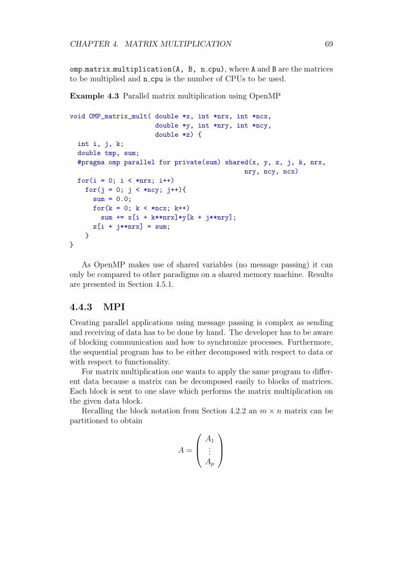
CHAPTER 4. MATRIX MULTIPLICATION 69
omp matrix multiplication(A, B, n cpu), where A and B are the matricesto be multiplied and n cpu is the number of CPUs to be used.
Example 4.3 Parallel matrix multiplication using OpenMP
void OMP_matrix_mult( double *x, int *nrx, int *ncx,double *y, int *nry, int *ncy,double *z) {
int i, j, k;double tmp, sum;#pragma omp parallel for private(sum) shared(x, y, z, j, k, nrx,
nry, ncy, ncx)for(i = 0; i < *nrx; i++)for(j = 0; j < *ncy; j++){sum = 0.0;for(k = 0; k < *ncx; k++)
sum += x[i + k**nrx]*y[k + j**nry];z[i + j**nrx] = sum;
}}
As OpenMP makes use of shared variables (no message passing) it canonly be compared to other paradigms on a shared memory machine. Resultsare presented in Section 4.5.1.
4.4.3 MPI
Creating parallel applications using message passing is complex as sendingand receiving of data has to be done by hand. The developer has to be awareof blocking communication and how to synchronize processes. Furthermore,the sequential program has to be either decomposed with respect to data orwith respect to functionality.
For matrix multiplication one wants to apply the same program to differ-ent data because a matrix can be decomposed easily to blocks of matrices.Each block is sent to one slave which performs the matrix multiplication onthe given data block.
Recalling the block notation from Section 4.2.2 an m× n matrix can bepartitioned to obtain
A =
A1...Ap

CHAPTER 4. MATRIX MULTIPLICATION 70
Ai is the ith block or sub matrix with dimensions mi by n of A where∑pi=1mi = m. We can say that A = Ai is an mi by n block matrix.The number of block matrices is given by the number p of available CPUs.
With this information given we can write down the matrix multiplication fora specific node:
Ci = AiB
Ci represents the local result of the multiplication. Clearly this is not thebest way to subdivide matrices in blocks (B has to be sent completely to allnodes) but is a good start to become familiar with data decomposition.
One issue, how many rows are sent to each slave, remains. If the numberof rows m of the matrix A can be evenly divided by the number of processorsp then m/p rows are sent to each slave. Otherwise the block matrices have tobe defined such that p− 1 slaves receive dm/pe and the remaining processorwill receive m− (p− 1)dm/pe rows.
This decomposition is used for the implementation of matrix multiplica-tion using MPI and PVM in paRc.
Implementation
We used the master-slave parallel programming paradigm (crowd computa-tion) to organize our tasks. This means that a master process exists whichis responsible for I/O, process spawning, distributing and collection of thedata. Only the slaves carry out the computation.
Package Rmpi is used to interface the MPI communication layer. Inaddition to the high level MPI multiplication routine provided by the packagesnow a separate implementation has been developed for package paRc tobecome familiar with message passing in MPI. The algorithms are presentedin this section.
Algorithm 3 shows the instructions to accomplish the task for the masterprocess and Algorithm 4 shows the instructions for the slaves. Whereas themaster is engaged with subdividing, sending, and collecting data, the slavesreceive their partition of matrix A—Arank, where rank is the identifier ofthe processor on which the slave runs on. After calculating the partial resultCrank, the master gathers them into the resulting matrix C.
Examples 4.4 and 4.5 show the R implementation of Algorithm 3 andAlgorithm 4 respectively. After validating the input n cpu number of R slavesare spawned. The master calculates and broadcasts all the necessary data tothe slaves. Then the slaves perform the actual computations and return theresulting local matrices to the master. The local solutions are combined toa single matrix which is the solution of the parallel matrix multiplication.
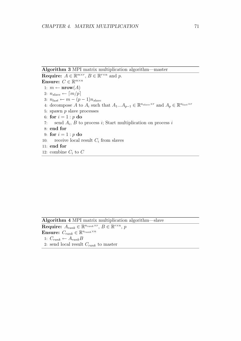
CHAPTER 4. MATRIX MULTIPLICATION 71
Algorithm 3 MPI matrix multiplication algorithm—master
Require: A ∈ Rm×r, B ∈ Rr×n and p.Ensure: C ∈ Rm×n
1: m← nrow(A)2: nslave ← dm/pe3: nlast ← m− (p− 1)nslave4: decompose A to Ai such that A1...Ap−1 ∈ Rnslave×r and Ap ∈ Rnlast×r
5: spawn p slave processes6: for i = 1 : p do7: send Ai, B to process i; Start multiplication on process i8: end for9: for i = 1 : p do
10: receive local result Ci from slaves11: end for12: combine Ci to C
Algorithm 4 MPI matrix multiplication algorithm—slave
Require: Arank ∈ Rnrank×r, B ∈ Rr×n, pEnsure: Crank ∈ Rnrank×n
1: Crank ← ArankB2: send local result Crank to master
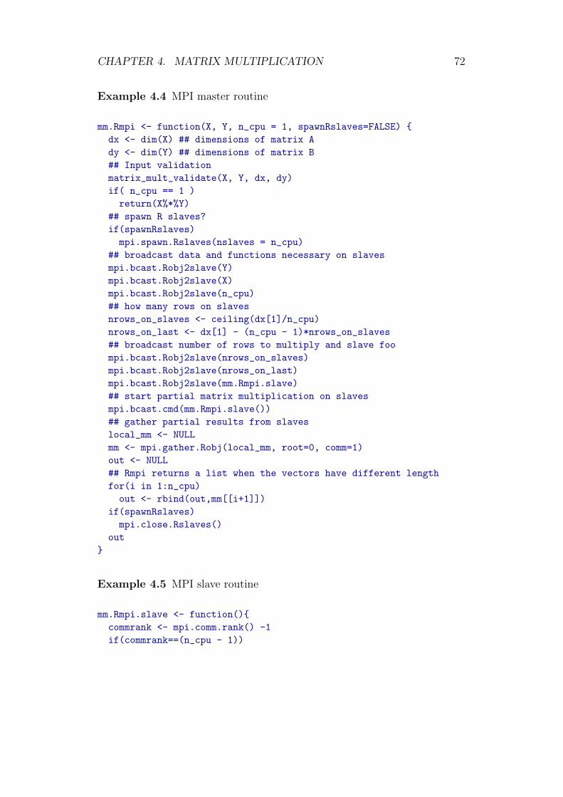
CHAPTER 4. MATRIX MULTIPLICATION 72
Example 4.4 MPI master routine
mm.Rmpi <- function(X, Y, n_cpu = 1, spawnRslaves=FALSE) {dx <- dim(X) ## dimensions of matrix Ady <- dim(Y) ## dimensions of matrix B## Input validationmatrix_mult_validate(X, Y, dx, dy)if( n_cpu == 1 )return(X%*%Y)
## spawn R slaves?if(spawnRslaves)mpi.spawn.Rslaves(nslaves = n_cpu)
## broadcast data and functions necessary on slavesmpi.bcast.Robj2slave(Y)mpi.bcast.Robj2slave(X)mpi.bcast.Robj2slave(n_cpu)## how many rows on slavesnrows_on_slaves <- ceiling(dx[1]/n_cpu)nrows_on_last <- dx[1] - (n_cpu - 1)*nrows_on_slaves## broadcast number of rows to multiply and slave foompi.bcast.Robj2slave(nrows_on_slaves)mpi.bcast.Robj2slave(nrows_on_last)mpi.bcast.Robj2slave(mm.Rmpi.slave)## start partial matrix multiplication on slavesmpi.bcast.cmd(mm.Rmpi.slave())## gather partial results from slaveslocal_mm <- NULLmm <- mpi.gather.Robj(local_mm, root=0, comm=1)out <- NULL## Rmpi returns a list when the vectors have different lengthfor(i in 1:n_cpu)out <- rbind(out,mm[[i+1]])
if(spawnRslaves)mpi.close.Rslaves()
out}
Example 4.5 MPI slave routine
mm.Rmpi.slave <- function(){commrank <- mpi.comm.rank() -1if(commrank==(n_cpu - 1))

CHAPTER 4. MATRIX MULTIPLICATION 73
local_mm <- X[(nrows_on_slaves*commrank + 1):(nrows_on_slaves*commrank + nrows_on_last),]%*%Y
elselocal_mm <- X[(nrows_on_slaves*commrank + 1):(nrows_on_slaves*
commrank + nrows_on_slaves),]%*%Ympi.gather.Robj(local_mm,root=0,comm=1)
}
4.4.4 PVM
PVM in R can be used with the package rpvm. In addition to the highlevel PVM multiplication routine provided by the package snow a separateimplementation has been developed for package paRc to become familiarwith message passing in PVM, which is slightly different from MPI.
Like the MPI implementation above the matrix multiplication is orga-nized according to the master-slave programming model. The difference toMPI is the lack of its ability to remotely execute commands. Therefore whenspawning R processes the complete source has to be available to the slave oncreation (i.e., from a file). The algorithms for matrix multiplication are thesame as shown in Section 4.4.3.
The PVM equivalents to the master and slave code of MPI are shown inExamples 4.6 and 4.7. After validating the input n cpu number of R slavesare spawned. Immediately after invoking this command the R slaves sourcethe code from a file "mm slave.R" (shown in Example 4.7). The master slavecalculates the necessary data and stores them in a buffer. This buffer is sendto all of the slaves. Then the slaves perform the actual computations (afterreceiving and unpacking the data of the buffer) and return the resulting localmatrices to the master. The local solutions are combined to a single matrixwhich is the solution of the parallel matrix multiplication.
Example 4.6 PVM master routine
mm.rpvm <- function(X, Y, n_cpu = 1) {dx <- dim(X) ## dimensions of matrix Xdy <- dim(Y) ## dimensions of matrix Y## Input validationmatrix_mult_validate(X,Y,dx,dy)## Tags for message sendingWORKTAG <- 17RESULTAG <- 82if(n_cpu == 1)

CHAPTER 4. MATRIX MULTIPLICATION 74
return(X%*%Y)mytid <- .PVM.mytid()children <- .PVM.spawnR(ntask = n_cpu, slave = "mm_slave.R")if (all(children < 0)) {cat("Failed to spawn any task: ", children, "\n").PVM.exit()
}else if (any(children < 0)) {cat("Failed to spawn some tasks. Successfully spawned ",
sum(children > 0), "tasks\n")children <- children[children > 0]
}nrows_on_slaves <- ceiling(dx[1]/n_cpu)nrows_on_last <- dx[1] - (n_cpu - 1)*nrows_on_slaves## distribute datafor (id in 1:length(children)) {.PVM.initsend().PVM.pkint(id).PVM.pkint(n_cpu).PVM.pkint(nrows_on_slaves).PVM.pkint(nrows_on_last).PVM.pkdblmat(X).PVM.pkdblmat(Y).PVM.send(children[id], WORKTAG)}## receive partial resultspartial_results <- list()for (child in children) {.PVM.recv(-1, RESULTAG)rank <- .PVM.upkint()partial_results[[rank]] <- .PVM.upkdblmat()
}.PVM.exit()## return in matrix formout <- NULLfor(i in 1:n_cpu)out <- rbind(out,partial_results[[i]])
out}
Eventually, the corresponding slave routine which actually carries out thewhole matrix multiplication looks as follows.

CHAPTER 4. MATRIX MULTIPLICATION 75
Example 4.7 PVM slave routine
library("rpvm")WORKTAG <- 17RESULTAG <- 82myparent <- .PVM.parent ()## Receive work from parent (a matrix)buf <- .PVM.recv (myparent, WORKTAG)rank <- .PVM.upkint() - 1n_cpu <- .PVM.upkint()nrows_on_slaves <- .PVM.upkint()nrows_on_last <- .PVM.upkint()X <- .PVM.upkdblmat()Y <- .PVM.upkdblmat()if(rank==(n_cpu - 1))
local_mm <- X[(nrows_on_slaves*rank + 1):(nrows_on_slaves*rank +nrows_on_last),]%*%Y
if(rank<(n_cpu - 1))local_mm <- X[(nrows_on_slaves*rank + 1):(nrows_on_slaves*rank +
nrows_on_slaves),]%*%Y## Send result back.PVM.initsend().PVM.pkint(rank + 1).PVM.pkdblmat(local_mm).PVM.send (myparent, RESULTAG)## Exit PVM.PVM.exit ()## Exit Rq (save="no")
4.5 Comparison of Parallel Routines
In this section the results of the comparison of parallel programming modelsare shown. They are compared on a shared memory machine using up to 4cores and on a distributed memory platform using up to 20 cluster nodes.On the shared memory machine matrices with dimensions of 1000 × 1000(complexity grade 1000) and 2500 × 2500 (complexity grade 2500) are usedand on the cluster nodes matrices with dimensions 2500× 2500 and 5000×5000 (complexity grade 5000).

CHAPTER 4. MATRIX MULTIPLICATION 76
4.5.1 Shared Memory Platform
On our shared memory testbed the number of available CPUs is restrictedto four. Benchmarks are run on the bignodes of cluster@WU.
Results of Complexity Grade 1000
Table 4.3 and Figure 4.1 show the resulting execution times of the matrix mul-tiplication with complexity grade 1000 (the dotted line represents the serialreference benchmark). A slight overhead is observed for the OpenMP routinefrom package paRc using one CPU but when increasing the number of CPUthis programming model scales better than the other two. This is becauseOpenMP makes use of shared variables and therefore not as much commu-nication overhead is produced as when using message passing—computationitself does not matter in relation to communication. Nevertheless, a slightoverhead produced from the compiler remains. This is what we expected. Inthis benchmark MPI and PVM show nearly the same speedup.
#CPU OpenMP MPI PVM7 1 7.43 7.18 7.20
14 2 3.71 3.97 5.0421 3 2.70 3.07 4.2228 4 2.14 2.60 3.97
Table 4.3: Comparison of parallel programming models on a shared memorymachine and complexity grade 1000
When using BLAS (as the supplied matrix multiplication routines fromsnow do) the results draw the following picture: Table 4.4 and Figure 4.2show that all of the programming models scale not so well. The commu-nication overhead is too large for this kind of complexity grade (the BLASroutines deliver results fast). Indeed, when using all computation cores thePVM routine from package snow is slower than with fewer cores. This isbecause the distribution of the data consumes more time with respect to thegain of distributing the computation.
Results of Complexity Grade 2500
Let the complexity be increased to 2500× 2500 matrices. Then, in contraryto 4.5.1 Figure 4.3 shows that the OpenMP routine performs worse thanthe other two. This is because the communication does not play an impor-tant role any more when carrying out this benchmark. The compiler driven
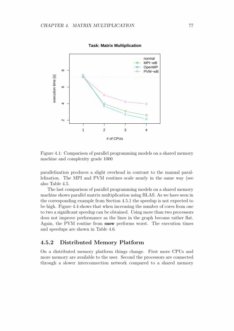
CHAPTER 4. MATRIX MULTIPLICATION 77
1 2 3 4
24
68
Task: Matrix Multiplication
# of CPUs
exec
utio
n tim
e [s
]
●
●
●
●
●
normalMPI−wBOpenMPPVM−wB
Figure 4.1: Comparison of parallel programming models on a shared memorymachine and complexity grade 1000
parallelization produces a slight overhead in contrast to the manual paral-lelization. The MPI and PVM routines scale nearly in the same way (seealso Table 4.5.
The last comparison of parallel programming models on a shared memorymachine shows parallel matrix multiplication using BLAS. As we have seen inthe corresponding example from Section 4.5.1 the speedup is not expected tobe high. Figure 4.4 shows that when increasing the number of cores from oneto two a significant speedup can be obtained. Using more than two processorsdoes not improve performance as the lines in the graph become rather flat.Again, the PVM routine from snow performs worst. The execution timesand speedups are shown in Table 4.6.
4.5.2 Distributed Memory Platform
On a distributed memory platform things change. First more CPUs andmore memory are available to the user. Second the processors are connectedthrough a slower interconnection network compared to a shared memory

CHAPTER 4. MATRIX MULTIPLICATION 78
#CPU MPI snow-MPI PVM snow-PVM3 1 2.55 2.56 2.56 2.56
12 2 1.66 1.81 1.14 1.8119 3 1.51 1.55 1.18 1.5426 4 1.38 1.68 1.43 1.49
Table 4.4: Comparison of parallel programming models on a shared memorymachine using BLAS and complexity grade 1000
#CPU OpenMP PVM6 1 142.63 141.12
11 2 70.45 59.9316 3 49.07 44.2321 4 40.10 35.43
Table 4.5: Comparison of parallel programming models on a shared memorymachine and complexity grade 2500
machine. This has an influence to all communication carried out in themessage passing environment. As we have more nodes available we decidedto use bigger matrices and therefore start with 2500×2500 and continue with5000× 5000 matrices.
Results of Complexity Grade 2500
Without using BLAS the MPI routine from package paRc scales rather well(Figure 4.5). The PVM routine shows good speedup until processor number 6but then performance gain breaks down. Again, PVM communication seemsto be suboptimal implemented.
Figure 4.6 is interesting. Only the MPI routine from paRc seems to de-liver good results. The PVM and the snow routines deliver lower performancewith increasing CPU counts after adding the 4th or 5th CPU. Furthermorethe snow PVM routine produced 2 outliers. It does not seem to deliver astable performance.
To sum up Table 4.7 shows the best results of the matrix multiplica-tion benchmark for each parallel programming model. It can be seen thatBLAS are highly optimized for the corresponding platform and can hardly bebeaten. Looking at the message passing models, the MPI routines performbetter with respect to the highest speedup which can be achieved than thePVM ones.

CHAPTER 4. MATRIX MULTIPLICATION 79
1 2 3 4
1.0
1.5
2.0
2.5
3.0
Task: Matrix Multiplication
# of CPUs
exec
utio
n tim
e [s
]
●
●
●
●
●
native−BLASMPIPVMsnow−MPIsnow−PVM
Figure 4.2: Comparison of parallel programming models on a shared memorymachine using BLAS and complexity grade 1000
Results of Complexity Grade 5000
The final task in this section is to multiply two 5000 × 5000 matrices onthe cluster nodes. Communication now really matters as one matrix needsaround 190 MB of memory when assuming that an entry is a double precisionfloating point of 8 Byte.
Figure 4.7 shows that the PVM routine has once more problems withlarge CPU counts. MPI is rather stable. Figure 4.8 shows the routines usingthe R BLAS library. Again PVM is unstable, the snow routines do not scalewell and MPI delivers stable and increasing performance.
Finally, Table 4.7 shows the best results of the matrix multiplicationbenchmark for each parallel programming model with complexity grade 5000.It can be seen that BLAS achieve again the best performance for the cor-responding platform (the disadvantages taken into consideration). In fact,comparing the best speedups which can be achieved for each programmingmodel draws the same picture as in Table 4.7: the MPI routines performbetter than the PVM routines. The message passing routine from packagepaRc seems to give a better speedup than the others.

CHAPTER 4. MATRIX MULTIPLICATION 80
1 2 3 4
5010
015
0
Task: Matrix Multiplication
# of CPUs
exec
utio
n tim
e [s
] ●
●
●
●
●
normalOpenMPPVM−wB
Figure 4.3: Comparison of parallel programming models on a shared memorymachine and complexity grade 2500
4.6 Conclusion
In this chapter we have shown how we achieved parallelism in R usingOpenMP and using message passing models like MPI and PVM. Further-more we compared the programming models on a shared and a distributedmemory platform.
On the shared memory platform we showed that OpenMP can be easyimplemented and that performance is rather good compared to the otherparallel programming models (when ignoring the optimized BLAS imple-mentations). Therefore we propose to use this paradigm for parallelizationof existing implementations in C as it is possible to incrementally parallelizecode. Then, as many commodity computers offer more than one processornowadays, one can experience higher performance when using R on a sharedmemory machine.
In contrast, on distributed memory platforms, one has to rely on messagepassing environments as they are by now the best way of achieving highperformance on these machines. It has been shown that MPI delivers better
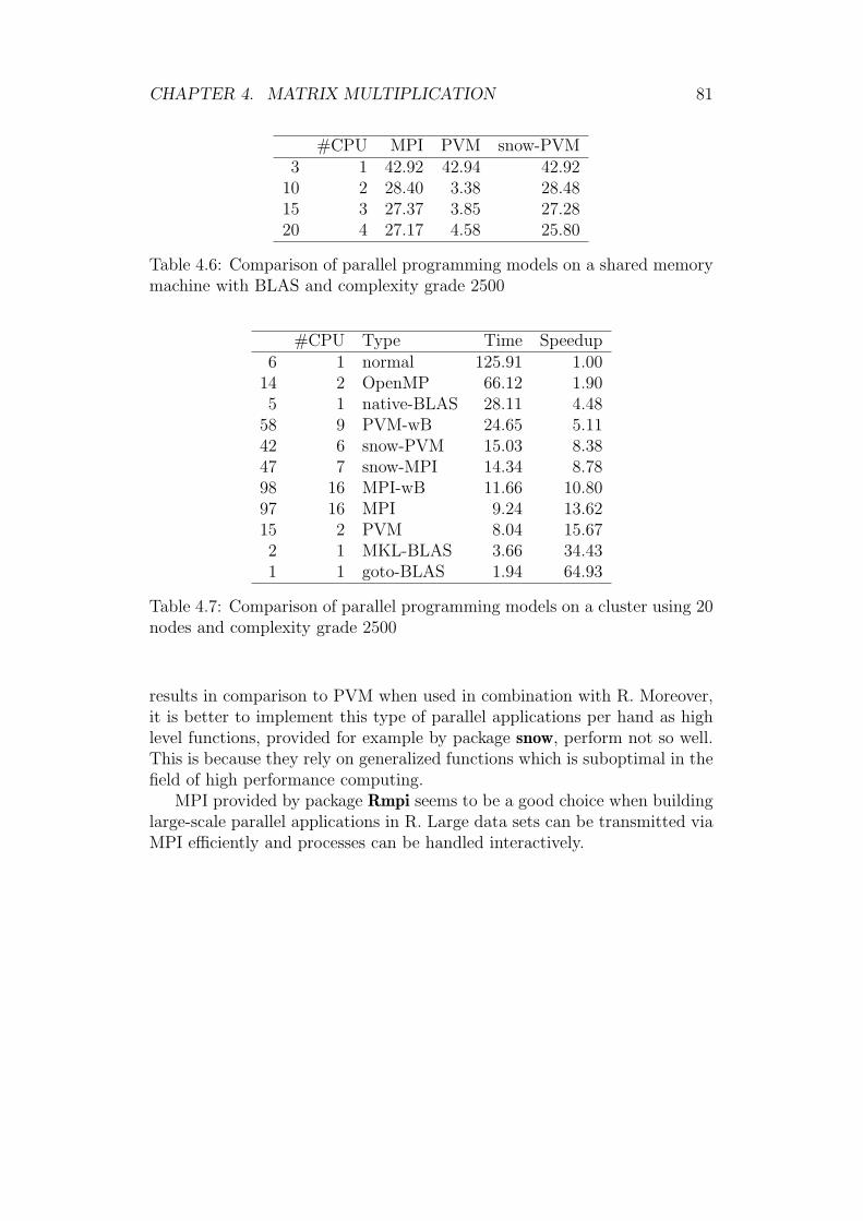
CHAPTER 4. MATRIX MULTIPLICATION 81
#CPU MPI PVM snow-PVM3 1 42.92 42.94 42.92
10 2 28.40 3.38 28.4815 3 27.37 3.85 27.2820 4 27.17 4.58 25.80
Table 4.6: Comparison of parallel programming models on a shared memorymachine with BLAS and complexity grade 2500
#CPU Type Time Speedup6 1 normal 125.91 1.00
14 2 OpenMP 66.12 1.905 1 native-BLAS 28.11 4.48
58 9 PVM-wB 24.65 5.1142 6 snow-PVM 15.03 8.3847 7 snow-MPI 14.34 8.7898 16 MPI-wB 11.66 10.8097 16 MPI 9.24 13.6215 2 PVM 8.04 15.672 1 MKL-BLAS 3.66 34.431 1 goto-BLAS 1.94 64.93
Table 4.7: Comparison of parallel programming models on a cluster using 20nodes and complexity grade 2500
results in comparison to PVM when used in combination with R. Moreover,it is better to implement this type of parallel applications per hand as highlevel functions, provided for example by package snow, perform not so well.This is because they rely on generalized functions which is suboptimal in thefield of high performance computing.
MPI provided by package Rmpi seems to be a good choice when buildinglarge-scale parallel applications in R. Large data sets can be transmitted viaMPI efficiently and processes can be handled interactively.

CHAPTER 4. MATRIX MULTIPLICATION 82
1 2 3 4
1.0
1.5
2.0
2.5
3.0
Task: Matrix Multiplication
# of CPUs
exec
utio
n tim
e [s
]
●
●
●
●
●
native−BLASMPIPVMsnow−PVM
Figure 4.4: Comparison of parallel programming models on a shared memorymachine with BLAS and complexity grade 2500
#CPU Type Time Speedup6 1 normal 1252.51 1.00
14 2 OpenMP 661.45 1.895 1 native-BLAS 222.61 5.63
40 6 PVM-wB 201.79 6.2159 9 snow-MPI 81.56 15.3666 10 snow-PVM 72.77 17.21
122 20 MPI-wB 64.10 19.54121 20 MPI 51.78 24.1915 2 PVM 35.29 35.492 1 MKL-BLAS 28.82 43.451 1 goto-BLAS 15.00 83.51
Table 4.8: Comparison of parallel programming models on a cluster using 20nodes and complexity grade 5000

CHAPTER 4. MATRIX MULTIPLICATION 83
0 5 10 15 20
5010
015
0
Task: Matrix Multiplication
# of CPUs
exec
utio
n tim
e [s
] ●
●
●
●●
● ● ● ● ● ● ● ● ● ● ● ● ● ● ●
●
normalMPI−wBOpenMPPVM−wB
Figure 4.5: Comparison of parallel programming models on a cluster using20 nodes and complexity grade 2500

CHAPTER 4. MATRIX MULTIPLICATION 84
0 5 10 15 20
1015
2025
3035
Task: Matrix Multiplication
# of CPUs
exec
utio
n tim
e [s
] ●●
●
●
●
● ●●
●● ● ● ● ● ● ●
● ● ● ●
●
native−BLASMPIPVMsnow−MPIsnow−PVM
Figure 4.6: Comparison of parallel programming models on a cluster using20 nodes using BLAS and complexity grade 2500
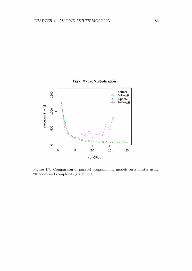
CHAPTER 4. MATRIX MULTIPLICATION 85
0 5 10 15 20
050
010
0015
00
Task: Matrix Multiplication
# of CPUs
exec
utio
n tim
e [s
]
●
●
●
●●
● ● ● ● ● ● ● ● ● ● ● ● ● ● ●
●
normalMPI−wBOpenMPPVM−wB
Figure 4.7: Comparison of parallel programming models on a cluster using20 nodes and complexity grade 5000

CHAPTER 4. MATRIX MULTIPLICATION 86
0 5 10 15 20
5010
015
020
025
030
0
Task: Matrix Multiplication
# of CPUs
exec
utio
n tim
e [s
] ●●
●
●
●
●●
● ● ● ● ● ● ● ● ● ● ● ● ●
●
native−BLASMPIPVMsnow−MPIsnow−PVM
Figure 4.8: Comparison of parallel programming paradigms on a cluster using20 nodes with BLAS and complexity grade 5000

Chapter 5
Option Pricing using ParallelMonte Carlo Simulation
5.1 Introduction
The search for competitive advantages and especially in economics and infinancial markets is in man’s nature. The biggest advantage a trader infinancial markets can have is to know something before all other market par-ticipants. On the stock exchange quickness and an advantage in time are thekey factors to be successful. On today’s financial markets more and moretrades are made by software and their algorithms (this is called algorith-mic trading) or even artificial intelligence (Kelly (2007)). A human tradercould process five to ten complex transactions per minute software in con-trast could process several thousand transactions per second and parallelismpreconditioned, look after several market places simultaneously.
The performance of the electronic exchange system is of great importancenowadays. Every millisecond counts and therefore financial firms keep theirtrading software as close to the trading system as possible (MacSweeney(2007)). This is because investors want to keep the time between the inputof a trade until its confirmation (this is called round tripping) at a minimum.Recently the Gruppe Deutsche Borse upgraded their trading system Xetra tooffer more bandwidth with lower latency (Gruppe Deutsche Borse (2007b),Gruppe Deutsche Borse (2007a)). These developments show the importanceof high performance computing in this sector.
In this chapter we investigate how high performance computing can beapplied in finance. This is done as a case study in which a European calloption is priced using parallel Monte Carlo simulation and the outcome iscompared to the analytical solution.
87
CHAPTER 5. PARALLEL MONTE CARLO SIMULATION 88
This chapter is organized as follows: First, a short overview of the theoryof option pricing is given, starting with a definition of derivatives and con-tinuing with the explanation of the Black-Scholes model. Then the theoryof Monte Carlo simulation of option prices is summarized. Before show-ing the results of the parallel Monte Carlo simulation the implementation isdescribed.
5.2 Option Pricing Theory
5.2.1 Derivatives
Derivatives are important in today’s financial markets. Futures and optionshave been increasingly traded since the last 20 years. Now, there are manydifferent types of derivatives.
A derivative is a financial instrument whose value depends on the valueof an other variable (or the values of other variables). This variable iscalled underlying.
Derivatives are traded on exchange-traded markets (people trade standard-ized contracts defined by the exchange) or over-the-counter markets (tradesare done in a computer linked network or over the phone—no physical con-tact).
There are two main types of derivatives, namely forwards (or futures) andoptions.
A forward is a contract in which one party buys (long position) or sells(short position) an asset at a certain time in the future for a certainprice. Futures in contrast are standardized and therefore are normallytraded on an exchange.
A call option is a contract which gives the holder the right to buy an assetat a certain time for a certain price (strike price).
A put option is a contract which gives the holder the right to sell an assetat a certain time for a certain price.
Forward prices (or future prices) can be determined in a simple way andtherefore it is not of computational interest for this chapter.
Options on the other hand are more sophisticated. There exist manyvariants of options on financial markets. European and American optionsare the most common of them.

CHAPTER 5. PARALLEL MONTE CARLO SIMULATION 89
European options are derivatives with the right to buy the underlying Sat a certain time T (expiration date or maturity) paying a previouslydefined price X (call option). If one sells this right it is called a putoption. Ct (Pt) denotes the value of the call option (put option) ata specific time t. St denotes the value of the underlying at a specifictime t. The price of a call option is defined as follows:
CT =
{0 if ST ≤ XST −X if ST > X,
}or max(ST −X, 0), (5.1)
and for the put option:
PT =
{0 if X ≤ STX − ST if X > ST
}or max(X − ST , 0). (5.2)
Figure 5.2.1 shows the payoff functions of a call and a put option andthe position of the investor (left: long position, right: short position).
American options are heavily traded on exchanges. The difference to itsEuropean counterpart is the fact, that it can be exercised at any time twithin the maturity 0 . . . T . The option expires if it is not exercised.The price of an American call option is
Ct =
{0 if St ≤ XSt −X if St > X,
}or max(St −X, 0), (5.3)
and for the put option:
Pt =
{0 if X ≤ StX − St if X > St
}or max(X − St, 0). (5.4)
In this chapter the pricing of European options is shown as we can obtainthe prices analytically (using the Black-Scholes-Merton model) and compareit to the prices estimated with Monte Carlo simulation.
5.2.2 Black-Scholes Model
In the 1970s Black and Scholes (1973) and Merton (1973) made a majorbreakthrough in the pricing of options. This soon became known as theBlack-Scholes model. They were awarded with the Nobel prize for economicsin 1997 for their work (Fischer Black died in 1995, otherwise he would havereceived this prize too).
In the model developed by Black, Scholes and Merton, price changes aredescribed mathematically by Markov processes. The Brownian motion (orWiener process) is one of the forms of Markov processes used as a model forstock price movements (this goes back to Bachelier (1900)).

CHAPTER 5. PARALLEL MONTE CARLO SIMULATION 90
60 80 100 120 140
020
40
European Call Option with Price 4
stock price
prof
it
60 80 100 120 140
−40
−20
0
European Call Option with Price 4
stock price
prof
it
60 80 100 120 140
020
40
European Put Option with Price 4
stock price
prof
it
60 80 100 120 140
−40
−20
0
European Put Option with Price 4
stock price
prof
it
Figure 5.1: Payoffs of a European put and call option depending on theposition of the investor
Brownian Motion or Wiener Process
A process (Wt)0≤t<∞ is a Brownian motion or a Wiener process if
1. W0 = 0,
2. the paths are continuous,
3. all increments Wt1 ,Wt2 − Wt1 , . . . ,Wtn − Wtn−1 are independent andnormal distributed for all 0 < t1 < t2 < · · · < tn
The Wiener process is a fundamental part of deriving option pricing for-mulas. An example of a Wiener path can be seen in Figure 5.2.2.
Stock Price Behavior
The value S of an underlying security follows the most widely used modelfor stock price behavior, the stochastic process
dS = µSdt+ σSdW (5.5)

CHAPTER 5. PARALLEL MONTE CARLO SIMULATION 91
Wiener Path
time
incr
emen
ts
0 1 2 3 4 5
−1.
5−
1.0
−0.
50.
00.
51.
0
Figure 5.2: Path of a Wiener process
ordS
S= µdt+ σdW
where µ is the drift rate (or expected return) and σ is the volatility. Wt isa standard Brownian motion and dt is a time increment. At t = 0 the valueS(0) is S0. If a volatility of zero is assumed the stock price would grow at acontinuously compounded rate of µ as
dS
S= µdt
and integrated between 0 and T is
ST = S0eµT .
Black-Scholes Differential Equation
Generally, the price of a derivative is a function of the stochastic variableunderlying the derivative (e.g., the stock S) and time t. In this case thestock price process is assumed to be like in Equation 5.5. If we suppose that
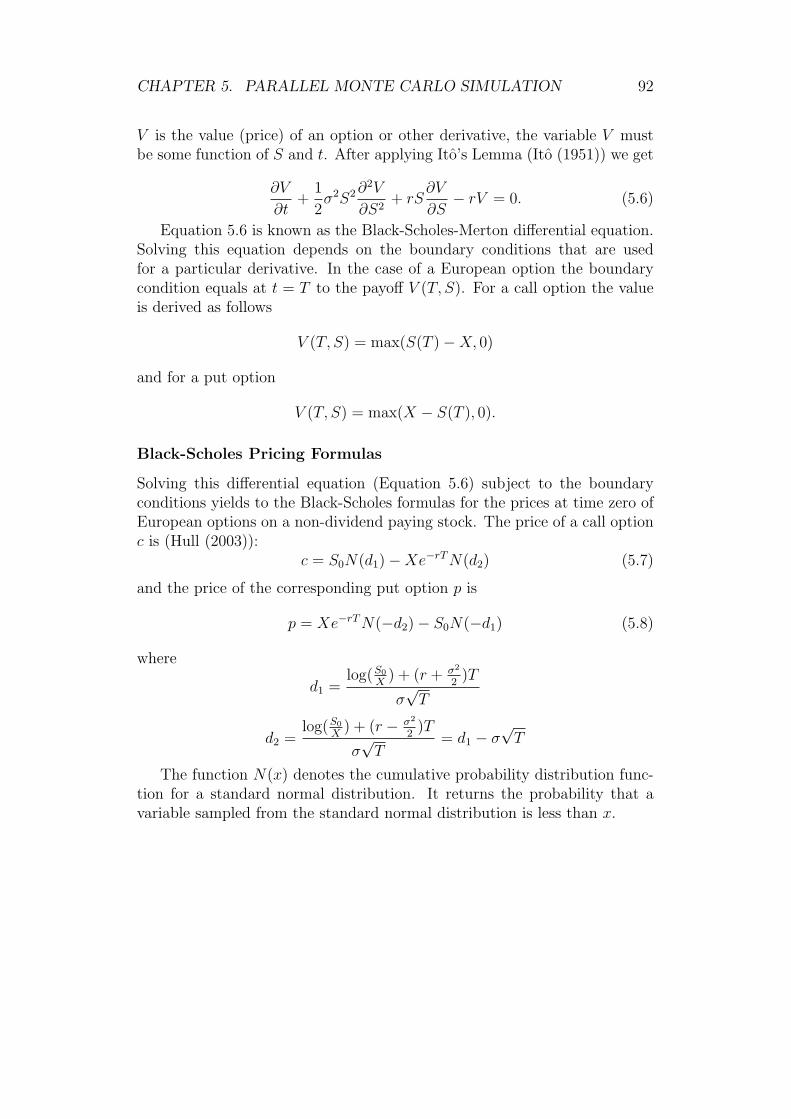
CHAPTER 5. PARALLEL MONTE CARLO SIMULATION 92
V is the value (price) of an option or other derivative, the variable V mustbe some function of S and t. After applying Ito’s Lemma (Ito (1951)) we get
∂V
∂t+
1
2σ2S2∂
2V
∂S2+ rS
∂V
∂S− rV = 0. (5.6)
Equation 5.6 is known as the Black-Scholes-Merton differential equation.Solving this equation depends on the boundary conditions that are usedfor a particular derivative. In the case of a European option the boundarycondition equals at t = T to the payoff V (T, S). For a call option the valueis derived as follows
V (T, S) = max(S(T )−X, 0)
and for a put option
V (T, S) = max(X − S(T ), 0).
Black-Scholes Pricing Formulas
Solving this differential equation (Equation 5.6) subject to the boundaryconditions yields to the Black-Scholes formulas for the prices at time zero ofEuropean options on a non-dividend paying stock. The price of a call optionc is (Hull (2003)):
c = S0N(d1)−Xe−rTN(d2) (5.7)
and the price of the corresponding put option p is
p = Xe−rTN(−d2)− S0N(−d1) (5.8)
where
d1 =log(S0
X) + (r + σ2
2)T
σ√T
d2 =log(S0
X) + (r − σ2
2)T
σ√T
= d1 − σ√T
The function N(x) denotes the cumulative probability distribution func-tion for a standard normal distribution. It returns the probability that avariable sampled from the standard normal distribution is less than x.

CHAPTER 5. PARALLEL MONTE CARLO SIMULATION 93
Risk Neutral Valuation
The assumption of a risk neutral world is one of the most important toolsfor the analysis of derivatives. This assumption can be derived from theBlack-Scholes differential equation as it does not involve any variable whichis affected by the risk preferences of investors (Hull (2003)).
In a world where investors are risk neutral, the expected return on allsecurities is the risk free rate of interest r. Therefore, the present value ofany cash flow can be obtained by discounting its expected value at the riskfree yield.
With this information given a derivative can be valued in a risk neutralworld by using the following important assumption: In a risk neutral worldthe return of the underlying asset (µ) is equal to the risk free interest rate (r).
Implementation in Package paRc
The Black-Scholes pricing formula is implemented in package paRc. If a Eu-ropean option is available one may call the function Black Scholes price(x,
r) to retrieve the exact price where x is an object of class ‘option’ and r isthe risk free yield.
Example 5.1 shows how the price of an European call option with strikeprice 100 and maturity 30 days (1/12 years) can be calculated using thefunction Black Scholes price(). The underlying is a stock with a currentvalue of 100, a µ of 0.1, and volatility σ of 0.4. The risk free yield is assumedto be 4.5%.
Example 5.1 Calculating the Black-Scholes price of an European option
> european <- define_option(c(0.1, 0.4, 100), 100, 1/12)> bsprice <- Black_Scholes_price(european, 0.1)> bsprice
value5.011784
The European options can be solved analytically as we saw in this section.Other derivatives can only be priced by numerical solutions. In the remainderof this chapter the use of Monte Carlo simulation is shown. Again we useEuropean options so that we can compare the analytical exact solution withthe numerical approximation.
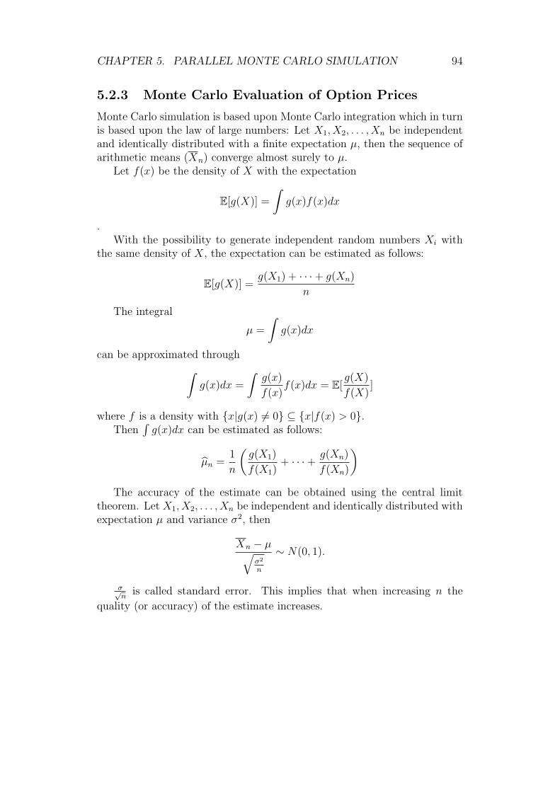
CHAPTER 5. PARALLEL MONTE CARLO SIMULATION 94
5.2.3 Monte Carlo Evaluation of Option Prices
Monte Carlo simulation is based upon Monte Carlo integration which in turnis based upon the law of large numbers: Let X1, X2, . . . , Xn be independentand identically distributed with a finite expectation µ, then the sequence ofarithmetic means (Xn) converge almost surely to µ.
Let f(x) be the density of X with the expectation
E[g(X)] =
∫g(x)f(x)dx
.With the possibility to generate independent random numbers Xi with
the same density of X, the expectation can be estimated as follows:
E[g(X)] =g(X1) + · · ·+ g(Xn)
n
The integral
µ =
∫g(x)dx
can be approximated through∫g(x)dx =
∫g(x)
f(x)f(x)dx = E[
g(X)
f(X)]
where f is a density with {x|g(x) 6= 0} ⊆ {x|f(x) > 0}.Then
∫g(x)dx can be estimated as follows:
µn =1
n
(g(X1)
f(X1)+ · · ·+ g(Xn)
f(Xn)
)The accuracy of the estimate can be obtained using the central limit
theorem. Let X1, X2, . . . , Xn be independent and identically distributed withexpectation µ and variance σ2, then
Xn − µ√σ2
n
∼ N(0, 1).
σ√n
is called standard error. This implies that when increasing n the
quality (or accuracy) of the estimate increases.

CHAPTER 5. PARALLEL MONTE CARLO SIMULATION 95
Simulating Paths of Stocks
The process of the underlying market value of a derivative is shown in Equa-tion 5.5. To simulate the path followed by S the time to maturity of theoption has to be subdivided into N short intervals of length δt and approxi-mate Equation 5.5 to
S(t+ δt)− S(t) = µS(t)δt+ σS(t)ε√δt
where S(t) denotes the value of S at time t, and ε is a random sample froma standard normal distribution. Now, for each δt all values of S can becalculated starting from the initial value S0. One simulation trial involvesconstructing a complete path for S using N random samples from a normaldistribution.
Usually it is more accurate to simulate ln S rather than S. This leads to
S(t+ δt) = S(t)e(bµ−σ2
2)δt+σε
√δt
Here the logarithm of the stock price is thus normally distributed, andthe stock price itself has a lognormal distribution. In contrast to the equationabove this equation is true for all δt.
The major advantage of Monte Carlo simulation is that the payoffs ofoptions can be simulated which depends not only on the final value of S butalso on the whole path followed by the underlying variable S. Furthermore,Monte Carlo simulation can be used to value options which depend on morethan one market variable. The drawbacks are that Monte Carlo simulationis computationally very time consuming but makes it in turn to a primeexample for parallel computing. A further disadvantage is that it cannoteasily handle situations where there are early exercise opportunities (e.g.,American options).
Variance Reduction Procedures
It is very expensive (in terms of computation time) to calculate the optionprice with Monte Carlo simulations as a very large number of simulation runsis necessary to estimate the price with reasonable accuracy. But there are anumber of variance reduction procedures available that can lead to savingsin computation time.
Among these variance reduction procedures there is a technique called an-tithetic variable. When using antithetic variable two values of the deriva-tive is calculated. One in the usual way (say f1) and the other using thesame random samples of the standard normal distribution but with inverse
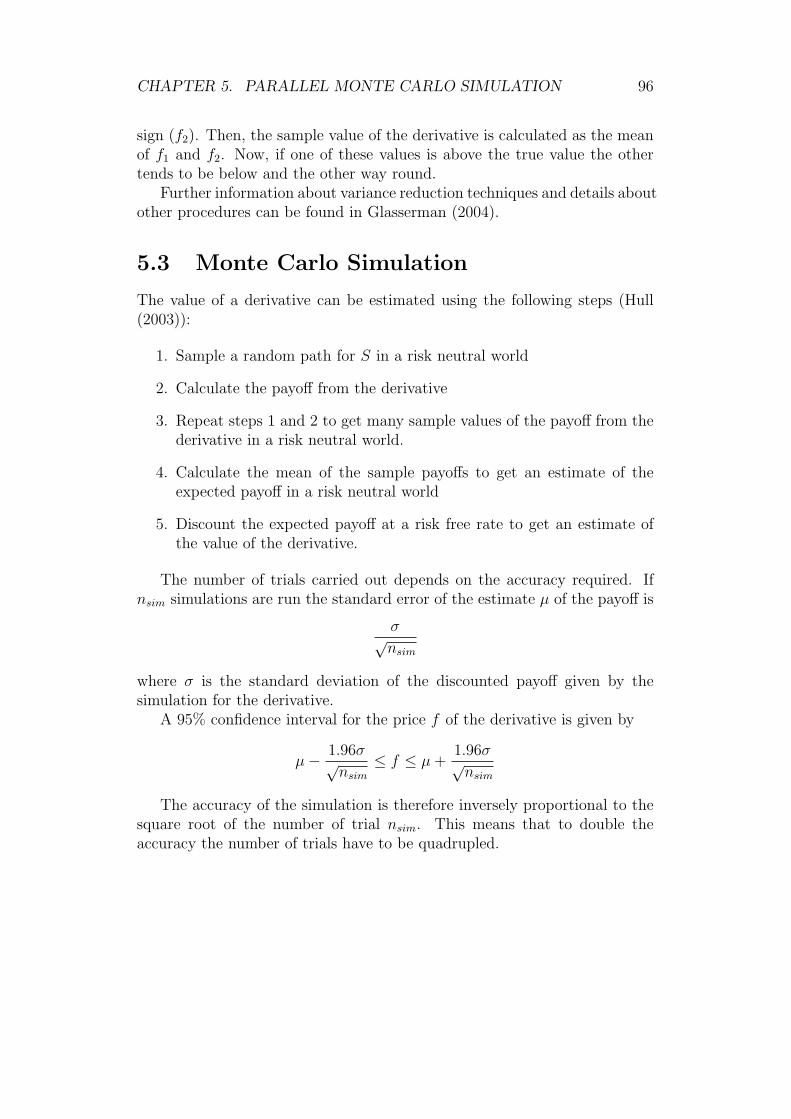
CHAPTER 5. PARALLEL MONTE CARLO SIMULATION 96
sign (f2). Then, the sample value of the derivative is calculated as the meanof f1 and f2. Now, if one of these values is above the true value the othertends to be below and the other way round.
Further information about variance reduction techniques and details aboutother procedures can be found in Glasserman (2004).
5.3 Monte Carlo Simulation
The value of a derivative can be estimated using the following steps (Hull(2003)):
1. Sample a random path for S in a risk neutral world
2. Calculate the payoff from the derivative
3. Repeat steps 1 and 2 to get many sample values of the payoff from thederivative in a risk neutral world.
4. Calculate the mean of the sample payoffs to get an estimate of theexpected payoff in a risk neutral world
5. Discount the expected payoff at a risk free rate to get an estimate ofthe value of the derivative.
The number of trials carried out depends on the accuracy required. Ifnsim simulations are run the standard error of the estimate µ of the payoff is
σ√nsim
where σ is the standard deviation of the discounted payoff given by thesimulation for the derivative.
A 95% confidence interval for the price f of the derivative is given by
µ− 1.96σ√nsim
≤ f ≤ µ+1.96σ√nsim
The accuracy of the simulation is therefore inversely proportional to thesquare root of the number of trial nsim. This means that to double theaccuracy the number of trials have to be quadrupled.
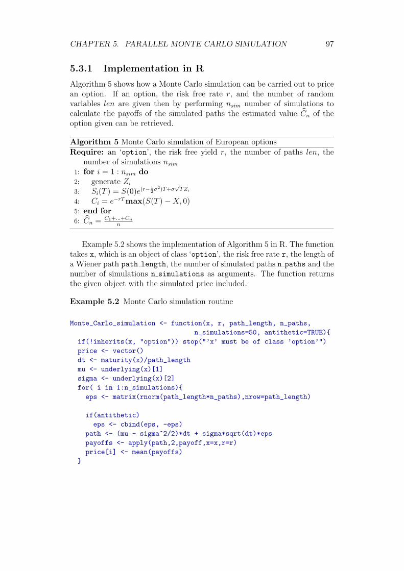
CHAPTER 5. PARALLEL MONTE CARLO SIMULATION 97
5.3.1 Implementation in R
Algorithm 5 shows how a Monte Carlo simulation can be carried out to pricean option. If an option, the risk free rate r, and the number of randomvariables len are given then by performing nsim number of simulations tocalculate the payoffs of the simulated paths the estimated value Cn of theoption given can be retrieved.
Algorithm 5 Monte Carlo simulation of European options
Require: an ‘option’, the risk free yield r, the number of paths len, thenumber of simulations nsim
1: for i = 1 : nsim do2: generate Zi3: Si(T ) = S(0)e(r−
12σ2)T+σ
√TZi
4: Ci = e−rTmax(S(T )−X, 0)5: end for6: Cn = C1+...+Cn
n
Example 5.2 shows the implementation of Algorithm 5 in R. The functiontakes x, which is an object of class ‘option’, the risk free rate r, the length ofa Wiener path path length, the number of simulated paths n paths and thenumber of simulations n simulations as arguments. The function returnsthe given object with the simulated price included.
Example 5.2 Monte Carlo simulation routine
Monte_Carlo_simulation <- function(x, r, path_length, n_paths,n_simulations=50, antithetic=TRUE){
if(!inherits(x, "option")) stop("’x’ must be of class ’option’")price <- vector()dt <- maturity(x)/path_lengthmu <- underlying(x)[1]sigma <- underlying(x)[2]for( i in 1:n_simulations){eps <- matrix(rnorm(path_length*n_paths),nrow=path_length)
if(antithetic)eps <- cbind(eps, -eps)
path <- (mu - sigma^2/2)*dt + sigma*sqrt(dt)*epspayoffs <- apply(path,2,payoff,x=x,r=r)price[i] <- mean(payoffs)
}

CHAPTER 5. PARALLEL MONTE CARLO SIMULATION 98
price_path(x) <- priceprice_of(x) <- mean(price)x
}
Recalling the option from Example 5.1 we can now use the functionMonte Carlo simulation() to estimate the price of the option. This isshown in Example 5.3 using a path length of 30 steps and 50 simulationruns. In each simulation run the mean of 5000 simulated payoffs is calcu-lated. Eventually the mean of the 50 estimated option prices and is storedin the object (see also the routine from Example 5.2).
Example 5.3 Estimating the price of an European option
> priced <- Monte_Carlo_simulation(european, r = 0.1,+ path_length = 30, n_paths = 5000)> priced
A Call option with strike price 100expiring in 30 daysCall price: 5.00535330924775
Table 5.1 shows estimates of the option price for three different numberof simulation runs and the corresponding runtime. Furthermore, the confi-dence interval of the estimate is calculated. It can be seen that even with alow number of trials it takes more than 10 seconds to finish the simulation.However, the standard error of the simulation is rather small for all results.The difference of the standard error between 50 and 150 trials is negligiblesmall.
The Convergence of the option price when increasing the number of sim-ulations can be seen in Figure 5.3. The grey line represents the Black-Scholesprice of the option.
#Sim MC estimate CI− CI+ Runtime[s]1 10.00 5.02 4.99 5.04 10.822 50.00 5.01 5.00 5.03 53.833 150.00 5.01 5.00 5.02 161.14
Table 5.1: Monte Carlo estimates and confidence intervals
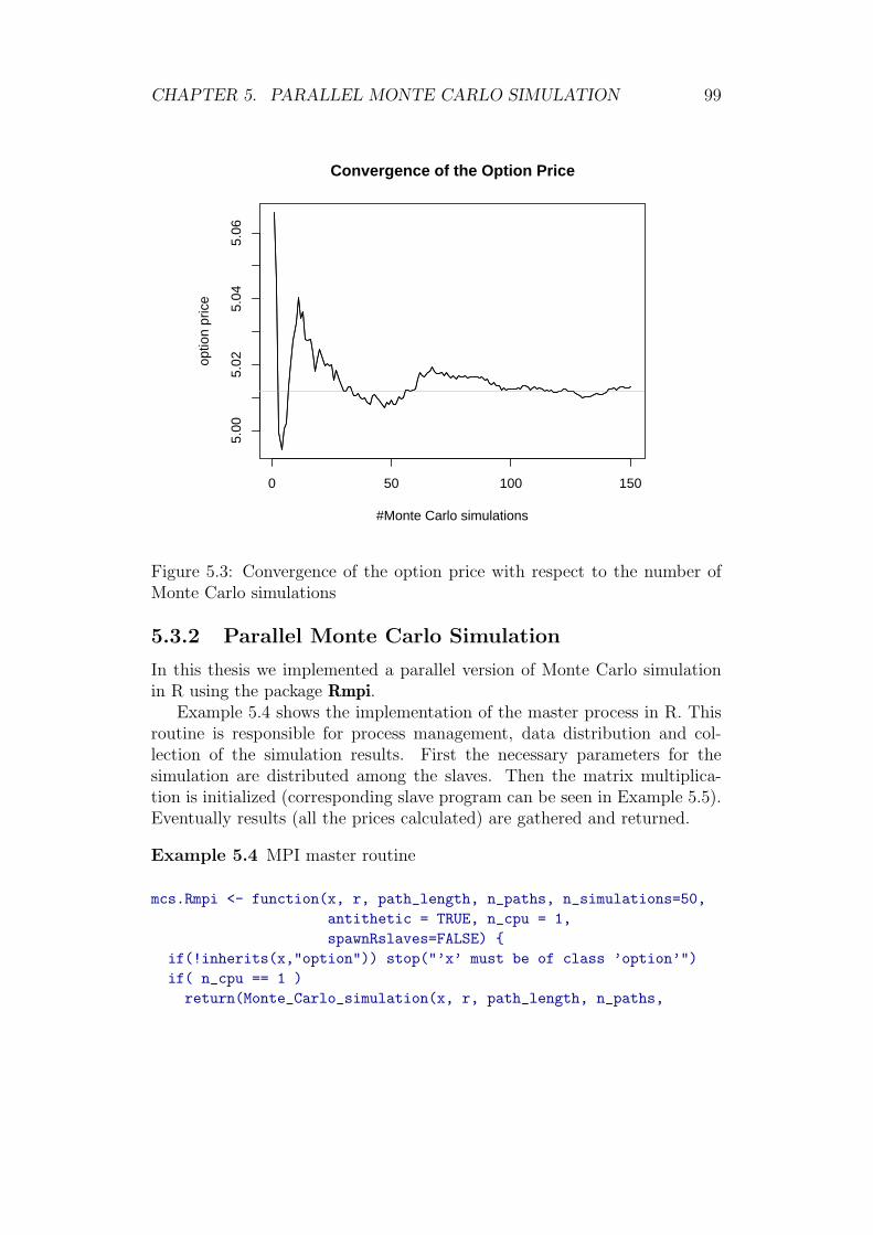
CHAPTER 5. PARALLEL MONTE CARLO SIMULATION 99
0 50 100 150
5.00
5.02
5.04
5.06
Convergence of the Option Price
#Monte Carlo simulations
optio
n pr
ice
Figure 5.3: Convergence of the option price with respect to the number ofMonte Carlo simulations
5.3.2 Parallel Monte Carlo Simulation
In this thesis we implemented a parallel version of Monte Carlo simulationin R using the package Rmpi.
Example 5.4 shows the implementation of the master process in R. Thisroutine is responsible for process management, data distribution and col-lection of the simulation results. First the necessary parameters for thesimulation are distributed among the slaves. Then the matrix multiplica-tion is initialized (corresponding slave program can be seen in Example 5.5).Eventually results (all the prices calculated) are gathered and returned.
Example 5.4 MPI master routine
mcs.Rmpi <- function(x, r, path_length, n_paths, n_simulations=50,antithetic = TRUE, n_cpu = 1,spawnRslaves=FALSE) {
if(!inherits(x,"option")) stop("’x’ must be of class ’option’")if( n_cpu == 1 )return(Monte_Carlo_simulation(x, r, path_length, n_paths,

CHAPTER 5. PARALLEL MONTE CARLO SIMULATION 100
n_simulations, antithetic))if(spawnRslaves)mpi.spawn.Rslaves(nslaves = n_cpu)
## broadcast data and functions necessary on slavesmpi.bcast.Robj2slave(x)mpi.bcast.Robj2slave(r)mpi.bcast.Robj2slave(path_length)mpi.bcast.Robj2slave(n_paths)mpi.bcast.Robj2slave(antithetic)nsim <- ceiling(n_simulations/n_cpu)nsim_on_last <- n_simulations - (n_cpu - 1)*nsimmpi.bcast.Robj2slave(nsim)mpi.bcast.Robj2slave(nsim_on_last)mpi.bcast.Robj2slave(mcs.Rmpi.slave)## start partial matrix multiplication on slavesmpi.bcast.cmd(mcs.Rmpi.slave())## gather partial results from slaveslocal_prices <- NULLprices <- mpi.gather.Robj(local_prices, root=0, comm=1)if(spawnRslaves)mpi.close.Rslaves()
prices}
The slave routine is basically the same like the serial version from Example 5.2except that it returns the local estimated prices to the master slave.
Example 5.5 MPI slave routine
mcs.Rmpi.slave <- function(){require("paRc")commrank <- mpi.comm.rank() - 1Monte_Carlo_slave <- function(x, r, path_length, n_paths,
n_simulations=50, antithetic=TRUE){price <- vector()dt <- maturity(x)/path_lengthmu <- underlying(x)[1]sigma <- underlying(x)[2]for( i in 1:n_simulations){eps <- matrix(rnorm(n*length),nrow=path_length)
if(antithetic)eps <- cbind(eps, -eps)

CHAPTER 5. PARALLEL MONTE CARLO SIMULATION 101
path <- (mu - sigma^2/2)*dt + sigma*sqrt(dt)*epspayoffs <- apply(path,2,payoff,x=x,r=r)price[i] <- mean(payoffs)
}price
}if(commrank==(n_cpu - 1))local_prices <- Monte_Carlo_slave(x, r, path_length, n_paths,
nsim_on_last, antithetic)elselocal_prices <- Monte_Carlo_slave(x, r, path_length, n_paths,
nsim, antithetic)mpi.gather.Robj(local_prices, root=0, comm=1)
}
5.3.3 Notes on Parallel Pseudo Random Number Gen-eration
Prior generating random numbers in parallel, a parallel pseudo random num-ber generator (PPRNG) has to be initialize (e.g., SPRNG is available in Rvia package rsprng). These generators assure that independend streams ofpseudo random numbers are available on the slaves (i.e., streams generatedon one node are independend and uncorrelated to streams generated on allof the other nodes). This is a crucial part for the quality of Monte Carlo esti-mates. Furthermore, the period length of generated random number streamshas to be long enough to cover the most sophisticated simulations and thegenerator itself has to be fast enough to be usable in high performance com-puting.
As already mentioned in Section 3.7 interfaces to widely used PPRNGare available in R (packages rsprng and rlecuyer).
5.3.4 Results of Parallel Monte Carlo Simulation
The results shown in this section were produced on a shared memory machineusing up to 4 cores (bignodes of cluster@WU) and on a distributed memoryplatform using up to 10 cluster nodes. We used 50 simulation runs to estimatethe option prices. The corresponding benchmark script can be found inAppendix C.
Figure 5.4 and Table 5.2 show that a good speedup can be achieved ona shared memory machine. Furthermore, in comparison to the results of theparallel matrix multiplication presented in Section 4.5 a better scalability is

CHAPTER 5. PARALLEL MONTE CARLO SIMULATION 102
#CPU Type Time Speedup1 1 normal 53.87 1.002 1 MPI 53.69 1.003 2 MPI 27.53 1.964 3 MPI 19.84 2.725 4 MPI 15.70 3.43
Table 5.2: Time and speedup achieved on a shared memory platform using50 simulation runs
#CPU Type Time Speedup1 1 normal 50.45 1.002 1 MPI 50.30 1.003 2 MPI 27.28 1.854 3 MPI 18.62 2.715 4 MPI 14.87 3.396 5 MPI 11.56 4.367 6 MPI 10.49 4.818 7 MPI 9.46 5.339 8 MPI 8.38 6.02
10 9 MPI 7.27 6.9411 10 MPI 6.19 8.16
Table 5.3: Time and speedup achieved on cluster@WU using 10 nodes and50 simulation runs
observed for both, using the shared memory paradigm and using the dis-tributed memory paradigm (Figure 5.5 and Table 5.3). This is because onlyfew data is sent through the interconnection network and therefore (withAmdahl’s law in mind) a greater fraction of the whole work can be executedin parallel. Moreover, when using the distributed memory paradigm only aslight overhead is observed in comparison to the shared memory paradigmbecause again of the fact that we have low communication costs.
To sum up, a substantial reduction of the execution time can be achievedwhen taking advantage of parallel computing. In fact we reduced the runtimeof the simulation from over 50 seconds necessary with one processor to nearly6 seconds using 10 processors (see Table 5.3).

CHAPTER 5. PARALLEL MONTE CARLO SIMULATION 103
1 2 3 4
2030
4050
6070
Task: Parallel Monte Carlo Simulation
# of CPUs
exec
utio
n tim
e [s
] ●
●
●
●
●
normalMPI
Figure 5.4: Performance of parallel Monte Carlo simulation using 50 simula-tion runs on a shared memory machine
5.4 Conclusion
In this chapter we presented a possible application of parallel computing incomputational finance–a field with an increasing demand for high perfor-mance computing.
Parallel Monte Carlo simulation makes extensive use of parallel randomnumber generators and therefore they have a major impact on the overallperformance. Further research is promising in this area as only few alter-natives exist. Furthermore, Monte Carlo simulation is not only an issue infinance but also for other problems which can only be solved numerically.
All in all in this case study we have shown that high scalability can beachieved for this type of application as work can nearly be perfectly dividedamong the slaves and only few data has to be sent via the network. Resultsshowed good speedups with increasing CPU counts.
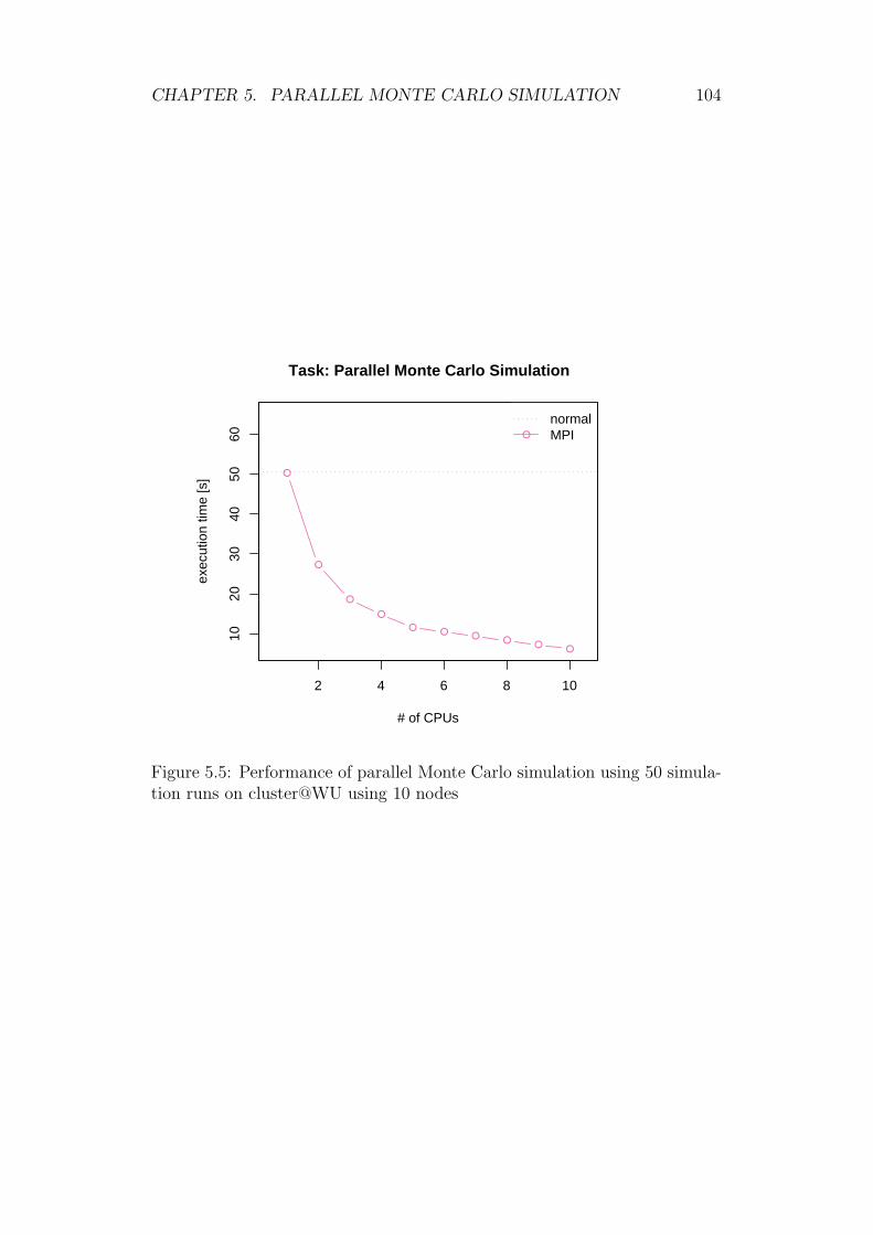
CHAPTER 5. PARALLEL MONTE CARLO SIMULATION 104
2 4 6 8 10
1020
3040
5060
Task: Parallel Monte Carlo Simulation
# of CPUs
exec
utio
n tim
e [s
] ●
●
●
●
●●
●●
●●
●
normalMPI
Figure 5.5: Performance of parallel Monte Carlo simulation using 50 simula-tion runs on cluster@WU using 10 nodes

Chapter 6
Conclusion and Future Work
6.1 Summary
The overview of the field of high performance computing presented in thefirst chapters is a good start to become familiar with the state of the art inhigh performance computing and in particular in parallel computing. Fur-thermore we presented in this thesis all relevant packages which extent thebase R environment with parallel computing facilities. All in all they are agood start to implement parallel routines although it is hard work to get rou-tines running with high stability. Nevertheless as algorithms become moretime consuming and problems in computational statistics become more dataintensive we propose to have at least a look on the possibilities which areoffered from parallel programming models.
With the introduction of OpenMP parallel programming has become eas-ier than ever. In this thesis we presented how one can only with a few state-ments parallelize existing serial code to achieve a significant reduction of theruntime. With R coming the restriction to low level languages like C orFORTRAN is a disadvantage. Therefore we propose implementing high levelinterface functions to efficient parallel OpenMP low level routines.
Using the benchmark environment provided by the package paRc showsthat high level functions designed for general use in parallel computing (likethe routines in snow) indeed help the user to achieve parallelism easily butwith the drawback of lower performance compared to specialized functions.
The second contribution of this thesis is the parallel implementation ofMonte Carlo simulation with a special focus on derivative pricing. Especiallyin finance, with the increasing importance of algorithmic trading, minimizingtime is of major interest. The need for cutting edge hardware of investmentcompanies and banks to minimize round tripping underlines this trend. Using
105

CHAPTER 6. CONCLUSION AND FUTURE WORK 106
high performance computing is becoming increasingly important in this fieldas parallel computers become mainstream
6.2 Economical Coherences
The economic principle has ever been maximizing profits. This means eitherraising of revenue, increasing the return or augmenting assets. In today’s everfaster society time has become an important figure. And indeed, minimizingtime to complete a task can be seen as some sort of profit. In view offinance e.g., saving time for calculating a trading strategy means an advancein knowledge and therefore can raise ones (monetary) profits as investorsmay respond earlier to market movements or as arbitrage earnings could begenerated.
In business administration optimization plays a major role. Actually incost accounting and controlling linear problems are solved using linear pro-gramming (e.g., to determine economic order quantities). In transportationone can think of automatic shortest path selection. Selecting an optimalpath is of major interest as it would maximize the deliveries possible in acertain time frame or prevent empty drives of trucks for example. The clas-sical example for this type of problems is the “travelling salesperson prob-lem”. Nevertheless, optimization is expensive in terms of computational timeand therefore it is desirable to have efficient (parallel) algorithms available.Parallel computing would be a possibility to achieve higher performance inoptimization.
Concluding we would like to say that we live in an economy which dependsmore and more on information technology. In the near future many ITcompanies will have to take the step from the serial to the parallel worldotherwise they will not benefit from the recent advances in this area (andthe research done in this area is even expected to increase). This also meansthat a major rethinking will have to take place in software development.
Nevertheless taking advantage of parallelism through dividing a problemin smaller (specialized) tasks is not a new idea in economics. Already a longtime ago one of the most important economists Smith (1776) proposed thedivision of labor to increase welfare. Now, it is time to divide tasks such thatcomputational time is minimized or in other words profit is increased.
CHAPTER 6. CONCLUSION AND FUTURE WORK 107
6.3 Outlook
High performance computing is applied to these tasks which are complexto solve and therefore need huge amount of computational time or for timecritical tasks where it is important to save every millisecond.
Today high performance computing is used in many scientific areas wheresophisticated computations are carried out. An important field which can beapplied in many fields in economics is optimization. NP-hard problems likedecision problems, search problems or as mentioned optimization problemsare solved in polynomial time. With parallel computing time could be re-duced to solve these problems provided that the problems can be subdividedaccordingly.
In this thesis classical examples like the matrix multiplication in parallelcomputing were shown. A lot of research has been done in this area toprovide even faster algorithms. A next step would be to implement themost promising variants (like the PUMMA) of them to become familiar withsophisticated parallel programming algorithms.
Many improvements are possible for package paRc. The benchmark en-vironment could be enhanced to provide greater flexibility to the user so thatnew benchmark alternatives can easily be integrated. Furthermore, new par-allel routines could be developed using the OpenMP programming model asan interface to the OpenMP library already exists.
Further research could clearly be done in the computational finance seg-ment. The recent advances in algorithmic trading and the increasing needfor computational power clearly indicate a trend towards high performancecomputing. The option pricing environment in package paRc supplies aframework for pricing derivatives using parallel Monte Carlo simulation whichmakes heavily use of parallel random number generators. A next step wouldbe to improve parallel pseudo random number generation. Only few researchhas been done in this area in the last years.
Besides the topics mentioned above, many more could be thought of andimplemented, thus there are more than enough fields for further research.
6.4 Acknowledgments
I was extremely lucky to carry out my diploma thesis at the Department ofStatistics and Mathematics. My position as a studies assistant gave me theopportunity to discuss many topics of this thesis with the staff members—mycolleagues. Especially I would like to thank my supervisor Kurt Hornik forhis guidance and mentorship and of course for the many reading.

CHAPTER 6. CONCLUSION AND FUTURE WORK 108
I would like to thank David Meyer as well as Achim Zeileis who helpedme with statistical, graphical and information technology issues.
Furthermore I would like to thank Josef Leydold for his hints regardingrandom number generation.
Last but not least, I would like to express my thanks to my parents fortheir ongoing encouragement. In addition I would like to thank my girlfriendSelma for proofreading and of course for her patience and her support.
Appendix A
Installation of Message PassingEnvironments
This appendix shows how one can set up an appropriate message passingenvironment and how this environment can be handled.
A.1 LAM/MPI
For installing LAM/MPI on a workstation or a cluster either the sourcecode or pre-compiled binaries can be downloaded from the project website(http://www.lam-mpi.org/). The source code can be compiled as follows(job script for SGE):
#$ -N compile-lam-gcc
## change to the source directory of downloaded LAM/MPI
cd /path/to/lamsource/
echo "#### clean ####"
make clean
echo "#### configure ####"
## configure - enable shared library support
./configure CC=gcc CXX=g++ FC=gfortran \
--prefix=/path/to/lamhome --enable-shared
echo "#### make ####"
make all
echo "#### install ####"
make install
echo "#### finished ####"
109

APPENDIX A. INSTALLATION OF MESSAGE PASSING ENVIRONMENTS110
If Debian Etch is used LAM/MPI can be installed using apt-get install
followed by the packages
lam-runtime LAM runtime environment for executing parallel programs,
lam4-dev Development of parallel programs using LAM,
lam4c2 Shared libraries used by LAM parallel programs.
To boot the LAM/MPI environment one can simply call lamboot fromthe command line. This sets up a 1 node “parallel” environment. To havemore nodes connected a configuration file has to be specified.
#
# example LAM host configuration file
# bhost.conf
#
#server.cluster.example.com schedule=no
localhost cpu=4
With this file given executing lamboot bhost.conf sets up a parallelenvironment with 4 nodes on localhost.
A.2 PVM
Building and installing the PVM daemon from source is explained extensivelyin the book of Geist et al. (1994).
If Debian Etch is used PVM can be installed using apt-get install
followed by the packages
pvm Parallel Virtual Machine - binaries
pvm-dev Parallel Virtual Machine - development files
libpvm3 Parallel Virtual Machine - shared libraries

Appendix B
Sun Grid Engine
A detailed documentation is available from the Sun Microsystems website(Sun Microsystems, Inc. (2007)). In this appendix the fundamental steps forrunning parallel routines with R are explained.
Important for running applications with the grid engine are job scripts.They work in the same way like shell scripts but additionally contain controlsequences for the grid engine. These control sequences always start with #$
followed by a command flag and an argument.Often used flags are:
-N defines that the following argument is the name of the job.
-q defines the queue to use.
-pe defines which parallel environment is to be started and how many nodeshave to be reserved.
B.1 LAM/MPI Parallel Environment
To use the LAM/MPI parallel environment (pe) with the grid engine thefollowing has to be inserted into the user’s .bashrc:
export LD_LIBRARY_PATH=/path/to/lamhome/lib:$LD_LIBRARY_PATH
export LAMHOME=/path/to/lamhome
where the paths point to the corresponding LAM/MPI installation.
111
APPENDIX B. SUN GRID ENGINE 112
Cluster Job Scripts
A job script for starting a LAM/MPI application looks like this:
#$ -N Rmpi-example
# use parallel environment lam with 12 nodes
#$ -pe lam 12
# run job on queue node.q to have a homogeneous processing
# environment
#$ -q node.q
R --vanilla < /path/to/my/Rmpi-example.R
This job of the name “Rmpi-example” starts a parallel LAM/MPI en-vironment with 12 nodes on node.q of cluster@WU. Eventually R is calledsourcing a specific file containing parallel R code.
B.2 PVM Parallel Environment
To use the PVM pe with the grid engine the following has to be inserted intothe user’s .bashrc:
# PVM>
# you may wish to use this for your own programs (edit the last
# part to point to a different directory f.e. ~/bin/_\$PVM_ARCH
#
if [ -z $PVM_ROOT ]; then
if [ -d /home/stheussl/lib/pvm3 ]; then
export PVM_ROOT=/home/stheussl/lib/pvm3
else
echo "Warning - PVM_ROOT not defined"
echo "To use PVM, define PVM_ROOT and
rerun your .bashrc"
fi
fi
if [ -n $PVM_ROOT ]; then
export PVM_ARCH=‘$PVM_ROOT/lib/pvmgetarch‘
APPENDIX B. SUN GRID ENGINE 113
# uncomment one of the following lines if you want the PVM
# commands directory to be added to your shell path.
#
export PATH=$PATH:$PVM_ROOT/lib # generic
export PATH=$PATH:$PVM_ROOT/lib/$PVM_ARCH # arch-specific
#
# uncomment the following line if you want the PVM
# executable directory to be added to your shell path.
#
export PATH=$PATH:$PVM_ROOT/bin/$PVM_ARCH
fi
Cluster Job Scripts
A job script for starting a PVM application looks like this:
#$ -N rpvm-test
# use parallel environment pvm with 8 nodes
#$ -pe pvm 8
# run job on queue node.q to have a homogeneous processing
# environment
#$ -q node.q
R --vanilla < /path/to/my/rpvm-example.R
This job of the name “rpvm-test” starts a parallel PVM environmentwith 12 nodes on node.q of cluster@WU. Eventually R is called sourcing aspecific file containing parallel R code.

Appendix C
Benchmark Definitions
In this appendix the benchmark source files and job scripts are shown.
C.1 Matrix Multiplication
Uniformly Distributed Matrices
In general we used the uniform distribution ([−5, 5]) to run the benchmark inthis thesis. The code for running a benchmark on a distributed memory ma-chine and a detailed description can be found in Section 4.4.1. The followingcode describes a benchmark for a shared memory machine.
## load required librarieslibrary("Rmpi")library("paRc")library("snow")
## definition of benchmarkmax_cpu <- 4task <- "matrix multiplication"taskID <- "mm"paradigm <- "shared"types <- c("OpenMP", "MPI","snow-MPI", "MPI-wB")complexity <- c(1000, 2500)runs <- 250## data descriptionbmdata <- list()bmdata[[1]] <- bmdata[[2]] <- 1000bmdata[[3]] <- function(x){
runif(x,-5,5)}
114
APPENDIX C. BENCHMARK DEFINITIONS 115
## create benchmark objectbm <- create_benchmark(task=task, data=bmdata,
type=types[1], parallel=TRUE,cpu_range=1:max_cpu, runs=runs)
set.seed(1782)## for each complexity and type run a number of benchmarksfor(n in complexity){
bmdata[[1]] <- bmdata[[2]] <- nbenchmark_data(bm) <- bmdatafor(type in types){benchmark_type(bm) <- typewriteLines(paste("Starting",type,"benchmark with complexity",n,
"..."))results <- run_benchmark(bm)save(results,file=sprintf("%s-%s-%s-%d.Rda", paradigm, taskID,
type, n))}
}
and the corresponding cluster job script looks as follows:
#$ -N MPI-distr-MM
#$ -pe lam 20
#$ -q node.q
/path/to/R-binary --vanilla < \
/path/to/MPI-benchmark-examples/distributed-mm.R
Normally Distributed Matrices
When using normally distributed entries in the matrices we used the followingbenchmark definition to run on a distributed memory machine:
## load required librarieslibrary("rpvm")library("paRc")library("snow")
## definition of benchmark runmax_cpu <- 20task <- "matrix multiplication"taskID <- "mm-norm"paradigm <- "distributed"
APPENDIX C. BENCHMARK DEFINITIONS 116
types <- c("PVM","snow-PVM")complexity <- c(1000, 2500, 5000)runs <- 250bmdata <- list()bmdata[[1]] <- bmdata[[2]] <- 1000bmdata[[3]] <- function(x){
rnorm(x)}
bm <- create_benchmark(task=task, data=bmdata,type=types[1], parallel=TRUE,cpu_range=1:max_cpu, runs=runs)
set.seed(1782)for(n in complexity){
bmdata[[1]] <- bmdata[[2]] <- nbenchmark_data(bm) <- bmdatafor(type in types){benchmark_type(bm) <- typewriteLines(paste("Starting",type,"benchmark with complexity",n,
"..."))results <- run_benchmark(bm)save(results,file=sprintf("%s-%s-%s-%d.Rda", paradigm, taskID,
type, n))}
}
and the corresponding job script for the grid engine looks as follows:
#$ -N PVM-norm-distr-MM
#$ -pe pvm 20
#$ -q node.q
/path/to/R-binary --vanilla < \
/path/to/PVM-benchmark-examples/distributed-mm.R
C.2 Option Pricing
To benchmark parallel Monte Carlo simulations the following code was used:
## load required librarieslibrary("Rmpi")library("paRc")

APPENDIX C. BENCHMARK DEFINITIONS 117
## definition of benchmark runmax_cpu <- mpi.universe.size()task <- "Monte Carlo simulation"taskID <- "mcs"paradigm <- "distributed"types <- c("normal", "MPI")runs <- 10
bm <- create_benchmark(task=task, data=list(),type=types[1], paralle=TRUE,cpu_range=1:max_cpu, runs=runs)
## define optionopt <- define_option(c(0.1,0.4,100),100,1/12)
bmdata <- list()bmdata[[1]] <- optbmdata[[2]] <- 0.1 ## yieldbmdata[[3]] <- 30 ## path lengthbmdata[[4]] <- 5000 ## number of pathsbmdata[[5]] <- 50 ## number of simulationsbmdata[[6]] <- TRUE ## use antitheticbenchmark_data(bm) <- bmdata
for(type in types){benchmark_type(bm) <- typewriteLines(paste("Starting",type,"benchmark..."))results <- run_benchmark(bm)save(results,file=sprintf("%s-%s-%s-%d.Rda", paradigm, taskID,
type, n))}
the corresponding job script looks as follows:
#$ -N MPI-distr-MCS
#$ -pe lam 10
#$ -q node.q
/path/to/R-binary --vanilla < \
/path/to/MPI-benchmark-examples/distributed-mcs.R

List of Figures
2.1 Amdahl’s Law for parallel computing . . . . . . . . . . . . . . 28
3.1 Payoff of a European call option with price 5.93 . . . . . . . . 58
4.1 Comparison of parallel programming models on a shared mem-ory machine and complexity grade 1000 . . . . . . . . . . . . . 77
4.2 Comparison of parallel programming models on a shared mem-ory machine using BLAS and complexity grade 1000 . . . . . . 79
4.3 Comparison of parallel programming models on a shared mem-ory machine and complexity grade 2500 . . . . . . . . . . . . . 80
4.4 Comparison of parallel programming models on a shared mem-ory machine with BLAS and complexity grade 2500 . . . . . . 82
4.5 Comparison of parallel programming models on a cluster using20 nodes and complexity grade 2500 . . . . . . . . . . . . . . . 83
4.6 Comparison of parallel programming models on a cluster using20 nodes using BLAS and complexity grade 2500 . . . . . . . 84
4.7 Comparison of parallel programming models on a cluster using20 nodes and complexity grade 5000 . . . . . . . . . . . . . . . 85
4.8 Comparison of parallel programming paradigms on a clusterusing 20 nodes with BLAS and complexity grade 5000 . . . . . 86
5.1 Payoffs of a European put and call option depending on theposition of the investor . . . . . . . . . . . . . . . . . . . . . . 90
5.2 Path of a Wiener process . . . . . . . . . . . . . . . . . . . . . 915.3 Convergence of the option price with respect to the number of
Monte Carlo simulations . . . . . . . . . . . . . . . . . . . . . 995.4 Performance of parallel Monte Carlo simulation using 50 sim-
ulation runs on a shared memory machine . . . . . . . . . . . 1035.5 Performance of parallel Monte Carlo simulation using 50 sim-
ulation runs on cluster@WU using 10 nodes . . . . . . . . . . 104
118
List of Tables
2.1 Interleaved concurrency . . . . . . . . . . . . . . . . . . . . . . 62.2 Parallelism . . . . . . . . . . . . . . . . . . . . . . . . . . . . . 62.3 Pipelining . . . . . . . . . . . . . . . . . . . . . . . . . . . . . 102.4 cluster@WU specification . . . . . . . . . . . . . . . . . . . . . 292.5 Opteron server specification . . . . . . . . . . . . . . . . . . . 29
4.1 Comparison of BLAS routines on a bignode with complexitygrade 1000 . . . . . . . . . . . . . . . . . . . . . . . . . . . . . 65
4.2 Comparison of BLAS routines on a bignode with complexitygrade 2500 . . . . . . . . . . . . . . . . . . . . . . . . . . . . . 65
4.3 Comparison of parallel programming models on a shared mem-ory machine and complexity grade 1000 . . . . . . . . . . . . . 76
4.4 Comparison of parallel programming models on a shared mem-ory machine using BLAS and complexity grade 1000 . . . . . . 78
4.5 Comparison of parallel programming models on a shared mem-ory machine and complexity grade 2500 . . . . . . . . . . . . . 78
4.6 Comparison of parallel programming models on a shared mem-ory machine with BLAS and complexity grade 2500 . . . . . . 81
4.7 Comparison of parallel programming models on a cluster using20 nodes and complexity grade 2500 . . . . . . . . . . . . . . . 81
4.8 Comparison of parallel programming models on a cluster using20 nodes and complexity grade 5000 . . . . . . . . . . . . . . . 82
5.1 Monte Carlo estimates and confidence intervals . . . . . . . . 985.2 Time and speedup achieved on a shared memory platform us-
ing 50 simulation runs . . . . . . . . . . . . . . . . . . . . . . 1025.3 Time and speedup achieved on cluster@WU using 10 nodes
and 50 simulation runs . . . . . . . . . . . . . . . . . . . . . . 102
119

Bibliography
Gene Amdahl. Validity of the Single Processor Approach to Achieving LargeScale Computing Capabilities. AFIPS Conference Proceedings, 30(8):483–485, 1967.
D.P. Anderson, J. Cobb, E. Korpela, M. Lebofsky, and D. Werthimer.SETI@home: an Experiment in Public-Resource Computing. Commu-nications of the ACM, 45(11):56–61, 2002.
Louis Bachelier. Theorie de la Speculation. PhD thesis, Gauthier-Villars,1900.
D.J. Becker, T. Sterling, D. Savarese, J.E. Dorband, U.A. Ranawak, andC.V. Packer. Beowulf: A Parallel Workstation for Scientific Computation.Proceedings of the 1995 International Conference on Parallel Processing(ICPP), pages 11–14, 1995.
Fischer Black and Myron Scholes. The Pricing of Options and CorporateLiabilities. Journal of Political Economy, 81(3):637–654, 1973.
Greg Burns, Raja Daoud, and James Vaigl. LAM: An Open Cluster Environ-ment for MPI. Proceedings of Supercomputer Symposium ’94, 94:379–386,1994.
J.M. Chambers and T.J. Hastie. Statistical Models in S. CRC Press, Inc.Boca Raton, FL, USA, 1991.
Jaeyong Choi, Jack Dongarra, and David Walker. PUMMA: Parallel Uni-versal Matrix Multiplication Algorithms on Distributed Memory Concur-rent Computers. Technical report, ORNL/TM–12252, Oak Ridge NationalLab., TN (United States), 1993.
Duane Currie. papply: Parallel apply Function Using MPI, 2005. URL http:
//ace.acadiau.ca/math/ACMMaC/software/papply/. R package version0.1.
120

BIBLIOGRAPHY 121
L. Dagum. OpenMP: A Proposed Industry Standard API for Shared MemoryProgramming. OpenMP. org, 1997.
J.J. Dongarra, LS Blackford, J. Choi, A. Cleary, E. D’Azeuedo, J. Demmel,I. Dhillon, S. Hammarling, G. Henry, A. Petitet, et al. ScaLAPACK User’sGuide. Society for Industrial and Applied Mathematics (SIAM), 1997.
R. Duncan. A Survey of Parallel Computer Architectures. Computer, 23(2):5–16, 1990.
Michael Flynn. Some Computer Organizations and Their Effectiveness. IEEETransactions on Computers, 21(9):948–960, 1972.
Ian Foster and Carl Kesselman. Globus: a Metacomputing InfrastructureToolkit. International Journal of High Performance Computing Applica-tions, 11(2):115, 1997.
Ian Foster and Carl Kesselman, editors. The Grid: Blueprint for a NewComputing Infrastructure. Morgan Kaufmann Publishers, 1999.
G.C. Fox, S.W. Otto, and A.J.G. Hey. Matrix Algorithms on a HypercubeI: Matrix Multiplication. Parallel Computing, 4:17–31, 1987.
E. Gabriel, G.E. Fagg, G. Bosilca, T. Angskun, J.J. Dongarra, J.M. Squyres,V. Sahay, P. Kambadur, B. Barrett, A. Lumsdaine, et al. Open MPI:Goals, Concept, and Design of a Next Generation MPI Implementation.Proceedings, 11th European PVM/MPI Users’ Group Meeting, pages 97–104, 2004.
Narain Gehani and Andrew McGettrick, editors. Concurrent Programming.Addison-Wesley Publishing Company, 1988.
Al Geist, Adam Beguelin, Jack Dongarra, Weicheng Jiang, Robert Manchek,and Vaidy Sunderam. PVM: Parallel Virtual Machine—A Users’ Guideand Tutorial for Networked Parallel Computing. MIT Press, 1994.
GA Geist, JA Kohl, and PM Papadopoulos. PVM and MPI: a Comparisonof Features. Calculateurs Paralleles, 8(2):137–150, 1996.
W. Gentzsch et al. Sun Grid Engine: Towards Creating a Compute PowerGrid. Proceedings of the First IEEE/ACM International Symposium onCluster Computing and the Grid, 2002.
Paul Glasserman. Monte Carlo Methods in Financial Engineering. Springer,2004.

BIBLIOGRAPHY 122
G.H. Golub and C.F. Van Loan. Matrix Computations. Johns HopkinsUniversity Press Baltimore, MD, USA, 1996.
Kazushige Goto. GotoBLAS FAQ, 2007. URL http://www.tacc.utexas.
edu/resources/software/gotoblasfaq.php.
W. Gropp and E. Lusk. Goals Guiding Design: PVM and MPI. ClusterComputing, 2002. Proceedings. 2002 IEEE International Conference on,pages 257–265, 2002.
W. Gropp, E.L. Lusk, N. Doss, and A. Skjellum. A High-Performance,Portable Implementation of the MPI Message Passing Interface Standard.Parallel Computing, 22(6):789–828, 1996.
Gruppe Deutsche Borse. Deutsche Borse vervierfacht Netzwerkbandbreite furXetra, 2007a. URL http://www.deutsche-boerse.com. Press release.
Gruppe Deutsche Borse. Deutsche Borse bietet erweiterte Xetra-Handelsdaten mit geringerer Latenz, 2007b. URL http://www.
deutsche-boerse.com. Press release.
John Hennessy and David Patterson, editors. Computer Architecture—AQuantitative Approach. Morgan Kaufmann, 2007.
Jay Hoeflinger. Extending OpenMP* to Clusters. Intel Corporation, 2006.URL http://www.intel.com. White Paper.
Kurt Hornik. The R FAQ, 2007. URL http://CRAN.R-project.org/doc/
FAQ/R-FAQ.html. ISBN 3-900051-08-9.
John C. Hull. Options, Futures and Other Derivatives. Prentice Hall, 5edition, 2003.
R. Ihaka and R. Gentleman. R: A Language for Data Analysis and Graphics.Journal of Computational and Graphical Statistics, 5(3):299–314, 1996.
Intel Corporation. Intel C++ Compiler Documentation. Intel Corporation,2007a. URL www.intel.com.
Intel Corporation. Intel Fortran Compiler Documentation. Intel Corporation,2007b. URL www.intel.com.
Intel Corporation. Intel Math Kernel Library for Linux User’s Guide, 2007c.URL http://developer.intel.com.

BIBLIOGRAPHY 123
Kiyoshi Ito. On Stochastic Differential Equations. American MathematicalSociety, 1951.
J. Kahle, M. Day, H. Hofstee, C. Johns, T. Maeurer, and D. Shippy. Intro-duction to the Cell Multiprocessor, 2005. URL http://www.ibm.com.
Jason Kelly. Hal 9000-style machines, Kubrick’s fantasy, outwit traders, 2007.URL http://www.bloomberg.com.
Andreas Kleen. A NUMA API for Linux. Novell, Inc., 2005. URL http:
//www.novell.com. White Paper.
Erricos Kontoghiorghes, editor. Handbook of Parallel Computing and Statis-tics. Chapman & Hall, 2006.
E. Korpela, D. Werthimer, D. Anderson, J. Cobb, and M. Leboisky.SETI@Home—Massively Distributed Computing for SETI. Computing inScience & Engineering [see also IEEE Computational Science and Engi-neering], 3(1):78–83, 2001.
CL Lawson, RJ Hanson, DR Kincaid, and FT Krogh. Basic Linear Alge-bra Subprograms for Fortran Usage. ACM Transactions on MathematicalSoftware (TOMS), 5(3):308–323, 1979.
Peter Lazar and David Schoenfeld. biopara: Self-contained Parallel Systemfor R, 2006. R package version 1.4.
P. L’Ecuyer, R. Simard, E.J. Chen, and W.D. Kelton. An Object-OrientedRandom-Number Package With Many Long Streams and Substreams. Op-erations Research, 50(6), 2002.
Na (Michael) Li. rsprng: R Interface to SPRNG (Scalable Parallel RandomNumber Generators), 2007. URL http://www.r-project.org/,http:
//www.biostat.umn.edu/~nali/SoftwareListing.html. R package ver-sion 0.3-4.
Na (Michael) Li and Anthony Rossini. rpvm: R Interface to PVM (ParallelVirtual Machine), 2007. URL http://www.r-project.org/. R packageversion 1.0.2.
Greg MacSweeney. Pleasures and Pains of Cutting-Edge Technology, 2007.URL http://www.wstonline.com.

BIBLIOGRAPHY 124
M. Mascagni and A. Srinivasan. SPRNG: A Scalable Library for Pseudo Ran-dom Number Generation. ACM Transactions on Mathematical Software,26(3):436–461, 2000.
Robert Merton. Theory of Rational Option Pricing. Bell Journal of Eco-nomics and Management Science, 4:141–183, 1973.
Message Passing Interface Forum. MPI: A Message-Passing Interface Stan-dard, 1994.
Message Passing Interface Forum. MPI-2: Extensions to the Message-PassingInterface, 2003.
Gordon Moore. Cramming More Components Onto Integrated Circuits. Elec-tronics, 38(8), 1965.
J. Nieplocha, R.J. Harrison, and R.J. Littlefield. Global Arrays: A Nonuni-form Memory Access Programming Model for High-Performance Comput-ers. The Journal of Supercomputing, 10(2):169–189, 1996.
OpenMP Architecture Review Board. OpenMP Application Program Inter-face Version 2.5, 2005.
Peter Pacheco. Parallel Programming with MPI. Morgan Kaufmann, 1997.
R Development Core Team. Writing R Extensions. R Foundation for Statis-tical Computing, Vienna, Austria, 2007a. URL http://www.R-project.
org.
R Development Core Team. R: A Language and Environment for StatisticalComputing. R Foundation for Statistical Computing, Vienna, Austria,2007b. URL http://www.R-project.org. ISBN 3-900051-07-0.
Anthony Rossini, Luke Tierney, and Na Li. Simple Parallel Statistical Com-puting in R. UW Biostatistics Working Paper Series, (Working Paper193), 2003. URL http://www.bepress.com/uwbiostat/paper193.
Nagiza Samatova, Srikanth Yoginath, David Baues, and Guruprasad Kora.A Seamless Interface to Perform Parallel Computation on Linear Alge-bra Problems Using the ScaLAPACK Library, 2005. URL http://www.
aspect-sdm.org/Parallel-R. R package version 0.5.1.
Nagiza F. Samatova, David Bauer, and Srikanth Yoginath. taskPR:Task-Parallel R Package, 2004. URL http://www.aspect-sdm.org/
Parallel-R/. R package version 0.2.7.

BIBLIOGRAPHY 125
N.F. Samatova, M. Branstetter, A.R. Ganguly, R. Hettich, S. Khan, G. Kora,J. Li, X. Ma, C. Pan, A. Shoshani, et al. High Performance StatisticalComputing with Parallel R: Applications to Biology and Climate Mod-elling. Journal of Physics, pages 505–509, 2006.
Hana Sevcikova. Statistical Simulations on Parallel Computers. Journal ofComputational and Graphical Statistics, (13):886–906, 2004.
Hana Sevcikova and A. J. Rossini. snowFT: Fault Tolerant Simple Networkof Workstations, 2004a. R package version 0.0-2.
Hana Sevcikova and A.J. Rossini. Pragmatic Parallel Computing. Journalof Statistical Software, 2004b.
Hana Sevcikova and Tony Rossini. R Interface to RNG with Multiple Streams,2004c. R package version 0.1.
Adam Smith. An Inquiry Into the Nature and Causes of the Wealth of Na-tions. 1776.
Richard Stallman and the GCC Developer Community. Using the GNUCompiler Collection. The Free Software Foundation, 2007. URL http:
//gcc.gnu.org.
Sun Microsystems, Inc. Sun N1 Grid Engine 6.1 User’s Guide. Sun Mi-crosystems, Inc., Santa Clara, CA U.S.A., 2007. URL http://docs.sun.
com/app/docs/doc/820-0699?a=load.
Stefan Theussl. R-Forge User’s Manual, 2007a. URL http://download.
r-forge.r-project.org/manuals/R-Forge_Manual.pdf.
Stefan Theussl. paRc: paRallel Computations in R, 2007b. URL http:
//parc.r-forge.r-project.org. R package version 0.0-9.
Luke Tierney, Anthony Rossini, Na Li, and H. Sevcikova. snow: SimpleNetwork of Workstations, 2007. R package version 0.2-3.
Wikipedia. High performance computing — wikipedia, the free ency-clopedia, 2007a. URL http://en.wikipedia.org/w/index.php?title=
High-performance_computing&oldid=151017056. [Online; accessed 14-August-2007].
Wikipedia. Computational overhead — wikipedia, the free encyclo-pedia, 2007b. URL http://en.wikipedia.org/w/index.php?title=
Computational_overhead&oldid=130287492. [Online; accessed 28-August-2007].

BIBLIOGRAPHY 126
Gregory Wilson and Paul Lu, editors. Parallel Programming Using C++.The MIT Press, 1996.
S. Yoginath, NF Samatova, D. Bauer, G. Kora, G. Fann, and A. Geist.RScaLAPACK: High-Performance Parallel Statistical Computing with Rand ScaLAPACK. Proceedings of the 18th International Conference onParallel and Distributed Computing Systems, pages 12–14, 2005.
Hao Yu. Rmpi: Parallel Statistical Computing in R. R News, 2(2):10–14,2002.
Hao Yu. Rmpi: Interface (Wrapper) to MPI (Message-Passing Interface),2006. URL http://www.stats.uwo.ca/faculty/yu/Rmpi. R package ver-sion 0.5-3.