Applications of single-iteration Kirchhoff least-squares migration Lorenzo Casasanta, Francesco Perrone*, Graham Roberts, Andrew Ratcliffe, Karen Purcell, Arash JafarGandomi and Gordon Poole, CGG Summary It is well-known that standard migration is not a true inverse operation and is based on the adjoint of the forward modeling operator. Due to this approximation the resulting migrated image can often suffer from various artifacts and uneven illumination issues, especially in regions of complex geology. Least-squares depth migration approximates the inverse of the forward modeling and can be used to reduce these problems. We show two real data applications of a single-iteration (non-iterative) Kirchhoff least-squares depth migration process to highlight the benefits of this technique. Our first example demonstrates improved amplitude behavior of the least-squares migration results on an offshore Gabon data set. In the second example we show an efficient way to include attenuation in the least-squares migration process, and highlight a stable uplift in resolution and illumination compensation of the final image using a Central North Sea data set. Introduction In recent years, least-squares migration has again become an active topic in industry and academia, with a number of publications showing uplift on both synthetic and field data (Dong et al., 2012; Zhang et al., 2013; Fletcher et al., 2015; Valenciano et al., 2015; Duprat and Baina, 2016; Khalil et al., 2016; Wang et al., 2016; Casasanta et al., 2017; Wu et al., 2017). The promise of least-squares migration is to reduce the problems associated with standard migration being the adjoint of the forward modeling operator (Nemeth et al., 1999). In fact, the application to under-sampled and irregularly acquired seismic data causes migration noise and (swing) artifacts, as well as uneven illumination in the image (Huang et al., 2014). An appropriate pre-processing sequence can help mitigate these problems, but the underlying issue remains. The large dimensionality of the seismic imaging problem means the migration inverse is only realistically solved using an iterative, gradient-based, approach. However, this is a slow and costly process involving multiple iterations of migration and de-migration. Here we present results from a practical and efficient common-offset, single iteration, least-squares Kirchhoff migration, inspired by the general idea of using non-stationary matching filters to estimate the effect of the Hessian operator (Guitton, 2004). In this paper we briefly recap the least-squares migration equations and demonstrate the uplift on resulting AVO work from an offshore Gabon data set. Then we show how to include attenuation in the least-squares migration scheme to give

the overall effect of an attenuation-compensating prestack depth migration and highlight the improvement in both resolution and illumination on a Central North Sea data set. Least-squares migration If we denote the acquired seismic data by d, the subsurface reflectivity traces as r and the Kirchhoff modeling operator as L, then Kirchhoff forward modeling (or de-migration) can be written as a linear operator:

.Lrd (1) Solving the inverse problem clearly gives the desired subsurface reflectivity, r = L-1 d, but computation of the direct inverse is not feasible with realistic seismic acquisition. The common alternative is to apply the adjoint, LH, of the forward operator, L, in Equation (1) (Claerbout, 1992) to the acquired data, d:

,dLm H (2) where m is the Kirchhoff migrated image that, as a result of the adjoint operator, suffers from artifacts and illumination issues. Nemeth et al. (1999) developed a formulation to mitigate these effects through the minimization of a least-squares cost function, f(r) = ║ d – Lr ║2, that matches observed data with modeled (de-migrated) data to update the migrated image. The solution of the usual least-squares normal equations gives:

,1 dLLLr HH (3)

where LHL is generally referred to as the Hessian operator. As mentioned earlier, Equation (3) can be solved iteratively, but we see that substituting Equation (2) into (3) gives:

.1mLLr H (4)

Guitton (2004) proposed that the action of the inverse Hessian, (LHL)-1, can be estimated via non-stationary matching filters following a de-migration / re-migration process: the filters derived to match the re-migration back to the initial migration are then applied to the initial migrated image to give an estimate of the reflectivity (via Equation 4). The cost of this least-squares migration process, and its mechanics of de-migration / re-migration, is similar to those of a single iteration of iterative schemes. As a key part of this process, we are aided by the use of curvelet domain filters for improved stability and structural consistency in the matching (Wang et al., 2016).

Applications of single-iteration Kirchhoff least-squares migration

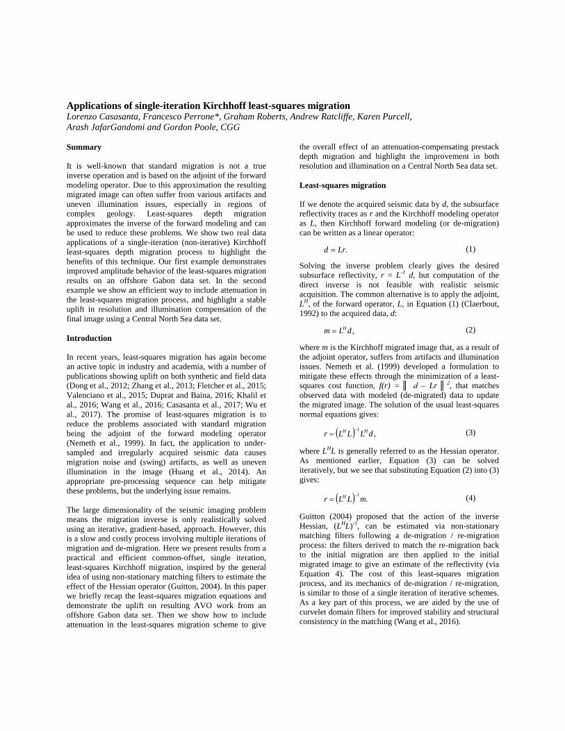
Offshore Gabon data example We demonstrate the single-iteration least-squares migration scheme on a 3D marine seismic data set acquired in the deep-water part of the South Gabon Basin. The survey was acquired using a variable-depth towed-streamer configuration for low-noise, broad-bandwidth data (Soubaras and Dowle, 2010). Previously we have shown that while the Kirchhoff depth migration provides detailed structural images, the presence of salt bodies result in cross-cutting swing artifacts and uneven illumination in some locations, together with speckled noise and reduced event coherency in the deep pre-salt region (Casasanta et al., 2017). Least-squares migration was seen to lessen the close-to-vertical migration swing artifacts and also, in general, to balance illumination, reduce noise and improve event coherency in the overall image. The changes in the migration artifacts, noise and illumination occur in each offset class and, hence, have an impact on the resulting AVO attributes. Figure 1 shows a comparison of the AVO gradient sections inverted from the standard and least-squares migration approaches, where the (qualitative) visual appearance is of a cleaner and more coherent AVO section. Unfortunately there is no well data available in this area to allow us to make a formal comparison of well and seismic reflectivity or AVO. However, a more quantitative analysis of this data is shown in the AVO cross-plots of Figure 2. Here we show intercept

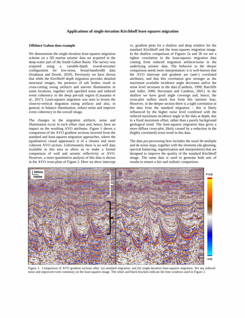
vs. gradient plots for a shallow and deep window for the standard Kirchhoff and the least-squares migration image. In the shallow comparison of Figures 2a and 2b we see a tighter correlation in the least-squares migration data coming from reduced migration artifacts/noise in the underlying seismic data. The behavior in the deeper comparison needs more interpretation: it is well-known that the AVO intercept and gradient are (anti-) correlated attributes, and that this correlation gets stronger as the maximum available incidence angle decreases and/or the noise level increases in the data (Cambois, 1998; Ratcliffe and Adler, 2000; Herrmann and Cambois, 2001). In the shallow we have good angle coverage and, hence, the cross-plot suffers much less from this intrinsic bias. However, in the deeper section there is a tight correlation in the data from the standard migration – this is likely influenced by the higher noise level combined with the reduced maximum incidence angle in the data at depth, due to a fixed maximum offset, rather than a purely background geological trend. The least-squares migration data gives a more diffuse cross-plot, likely caused by a reduction in the (highly correlated) noise trend in this data. The data pre-processing here includes the usual de-multiple and de-noise steps, together with the elements (de-ghosting, spectral balancing, regularization and interpolation) that are designed to improve the quality of the standard Kirchhoff image. The same data is used to generate both sets of results to ensure a fair and realistic comparison.

Figure 1: Comparison of AVO gradient sections after: (a) standard migration, and (b) single-iteration least-squares migration. We see reduced noise and improved event continuity on the least-squares image. The white and black brackets indicate the time windows used in Figure 2.

Applications of single-iteration Kirchhoff least-squares migration

Least-squares migration with attenuation The anelastic nature of the earth leads to absorption of seismic waves in the form of amplitude attenuation and phase distortion. Conventional acoustic migration assumes these effects are handled either pre- or post-migration. However, the quality factor that models absorption (Q for brevity) can be included in the standard migration to compensate for these effects (Xie et al., 2009). To include attenuation in the least-squares migration process, we modify the modeling Equation (1):

,rLd Q (5) where LQ now represents the Kirchhoff visco-acoustic modeling operator (Wu et al., 2017). Formulating a least-squares cost function, f(r) = ║ d – LQr ║2, and solving the normal equations gives a new version of Equation (3):

.1 dLLLr HQQ

HQ

(6)

Within the visco-acoustic Kirchhoff modeling operator (see Wu et al., 2017 for details), we highlight that the absorption can be modelled by a so-called dissipation function, D: )],/ln()/exp[(]2/exp[),,,( 0

** TiTxyxD rs where xs and xr are the shot and receiver coordinates, T* is the dissipation time (a function of velocity and Q), is the temporal frequency and 0 the Q reference frequency. This function contains a negative real exponential term to model amplitude attenuation and an imaginary exponential term to model the frequency-dependent phase distortion.

It is interesting to look at the mechanics of these equations to better understand the Kirchhoff visco-acoustic modeling operator, how it interacts in a least-squares scheme, and, also, contrasts with a Q-compensating migration. Starting with the flow in Equation (6), we note that the adjoint of the dissipation function still contains a negative real exponential term, i.e. still attenuates, but now has a sign-reversed imaginary exponential term for the phase restoration. Hence: (i) the acquired seismic data, d, is attenuated with a given imaginary exponential term for phase distortion due to Q absorption, (ii) the Kirchhoff visco-acoustic modeling operator, LQ, simulates the amplitude attenuation and phase distortion effects of the earth, and (iii) the adjoint of the Kirchhoff visco-acoustic modeling operator, LQ

H, again attenuates but with a sign-reversed imaginary exponential term to compensate for phase distortion. As a consequence, the Hessian term (LQ

H LQ) contains a double attenuation but has distorting and restoring phase behaviors that cancel within it, as does the data formed in the initial migrated image (LQ

H d). When we apply the inverse Hessian (which is a double amplitude boost) to the initial (double attenuated) migration we end up with an image that is free from the effects of Q. We note that, somewhat counterintuitively, this initial migration (LQ

H d) is not a Q-compensating migration, yet the least-squares flow delivers an overall Q-compensating behavior. Solving Equation (6) involves the application of Q in all the workflow steps: initial migration, de-migration and re-migration. In general, visco-ascoustic Kirchhoff forward and adjoint operators are more computationally demanding than their acoustic counterparts. This makes least-squares migration with attenuation a more expensive process. By stepping away from the least-square migration framework of Equation (6), one can design more cost effective approaches, involving the application of only one attenuating operator and conventional acoustic migrations/de-migrations (Y. Xie and P. Wang, personal communication, 2016). This new flow can be defined by:

,1 dLLLr HQ

H (7)

or ,1* dLLLr H

Q

(8) where the new symbol, LQ

*, denotes a migration operator with the same amplitude and phase behavior of the visco-acoustic modeling operator. Similar arguments to those discussed above on the mechanics also hold for the new flows in Equations (7) and (8): in these we highlight a key point related to the phase distortion term cancelling (as desired) because we use appropriate modeling and migration operators in these equations. Any Q behavior in these operators always attenuates and has a given exponential term for phase distortion due to Q absorption.

Figure 2: Comparison of AVO intercept (R0) vs. gradient (G) cross-plots for: (a) and (c) standard migration (blue), and (b) and (d) single-iteration least-squares migration (red) for the shallow and deep analysis time windows highlighted in Figure 1.

Applications of single-iteration Kirchhoff least-squares migration

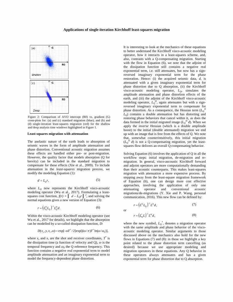
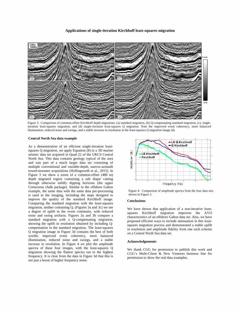
Central North Sea data example As a demonstration of an efficient single-iteration least-squares Q migration, we apply Equation (8) to a 3D marine seismic data set acquired in Quad 22 of the UKCS Central North Sea. This data contains geology typical of the area and was part of a much larger data set consisting of multiple conventional and variable-depth, narrow-azimuth towed-streamer acquisitions (Hollingworth et al., 2015). In Figure 3 we show a zoom of a common-offset (480 m) depth migrated region containing a salt diapir cutting through otherwise mildly dipping horizons (the upper Cretaceous chalk package). Similar to the offshore Gabon example, the same data with the same data pre-processing is used in the imaging, including the steps designed to improve the quality of the standard Kirchhoff image. Comparing the standard migration with the least-squares migration, neither containing Q, (Figures 3a and 3c) we see a degree of uplift in the event continuity, with reduced noise and swing artifacts. Figures 3a and 3b compare a standard migration with a Q-compensating migration, showing the uplift in resolution obtained by including Q-compensation in the standard migration. The least-squares Q migration image in Figure 3d contains the best of both worlds: improved event coherency, more balanced illumination, reduced noise and swings, and a stable increase in resolution. In Figure 4 we plot the amplitude spectra of these four images, with the least-squares Q migration showing the flattest spectra out to the highest frequency. It is clear from the data in Figure 3d that this is not just a boost of higher frequency noise.

Conclusions We have shown that application of a non-iterative least-squares Kirchhoff migration improves the AVO characteristics of an offshore Gabon data set. Also, we have proposed efficient ways to include attenuation in this least-squares migration process and demonstrated a stable uplift in resolution and amplitude fidelity from one such scheme on a Central North Sea data set. Acknowledgements We thank CGG for permission to publish this work and CGG’s Multi-Client & New Ventures business line for permission to show the real data examples.

Figure 3: Comparison of common-offset Kirchhoff depth migrations: (a) standard migration, (b) Q-compensating standard migration, (c), single-iteration least-squares migration, and (d) single-iteration least-squares Q migration. Note the improved event coherency, more balanced illumination, reduced noise and swings, and a stable increase in resolution in the least-squares Q migration image (d).

Figure 4: Comparison of amplitude spectra from the four data sets shown in Figure 3.