application of time preconditioning and high-order compact discretization method for low mach number...

INTERNATIONAL JOURNAL FOR NUMERICAL METHODS IN FLUIDSInt. J. Numer. Meth. Fluids 2013; 72:650–670Published online 20 Nov 2012 in Wiley Online Library (wileyonlinelibrary.com/journal/nmf). DOI: 10.1002/fld.3756

Application of time preconditioning and high-order compactdiscretization method for low Mach number flows

A. Tyliszczak1,*,† and H. Deconinck2

1Czestochowa University of Technology, Al. Armii Krajowej 21, 42-200 Czestochowa, Poland2von Karman Institute for Fluid Dynamics, Waterloosesteenweg, 72, B-1640 Sint-Genesius-Rode, Belgium

SUMMARY

The paper describes a combination of a preconditioning method with a high-order compact discretizationscheme for the purpose of solving the compressible Navier–Stokes equations in moderate and low Machnumber regimes. When combined with properly modified characteristic boundary conditions, the proposedapproach is very efficient from the point of view of convergence acceleration and accuracy of the results. Thecomputations were performed in typical benchmark cases including the Burggraf flow for which an analyti-cal solution exists, the flow over a backward facing step, and also the flow in 2D and 3D shear-driven cavities.Depending on the test case, the results were obtained for the Mach number in the range M D 0.001 � 0.5and the Reynolds number Re D 1� 1000. Copyright © 2012 John Wiley & Sons, Ltd.

Received 22 May 2012; Revised 4 October 2012; Accepted 28 October 2012

KEY WORDS: time preconditioning; compact scheme; characteristic boundary conditions; convergenceacceleration

1. INTRODUCTION

Numerical methods for compressible low Mach number flow have to cope with two fundamentalproblems. The first one is the stability constraint which for explicit time integration methods causesthe allowable numerical time step to scale proportionally with the Mach number, and so, the timestep approaches zero together with the Mach number. This has a direct consequence in both steadyand unsteady computations. The former are usually performed applying the so-called time-marchingalgorithm in which the time integration is continued as long as necessary to reach the steady, timeindependent solution. If the numerical time step approaches zero, the convergence of any explicittime-marching method is extremely slow. From the point of view of the convergence rate, any sys-tem of equations may be characterized by the so-called stiffness of the system determined basedon the condition number being the ratio of the maximum to minimum eigenvalue of the system.The general rule is the bigger the condition number, the stiffer is the system and more difficult tosolve. In the case of the compressible flow for the subsonic conditions, the maximum eigenvalue ofthe system is of the order of speed of sound, whereas the minimum eigenvalue is equal to the flowvelocity. When the Mach number approaches zero, the condition number goes to infinity and thesystem is regarded as very stiff, requiring either sophisticated numerical tools particularly designedfor stiff systems or a very huge number of iterations (time steps) if simple methods are used.

For unsteady computations, the convergence problem is less important but even in these cases,one may observe that unsteady phenomena requiring sufficient resolution from the physical pointof view are resolved at extremely high computational cost due to stability constrained time step

*Correspondence to: A. Tyliszczak, Czestochowa University of Technology, Al. Armii Krajowej 21, 42-200Czestochowa, Poland.

†E-mail: [email protected]

Copyright © 2012 John Wiley & Sons, Ltd.

APPLICATION OF TIME PRECONDITIONING AND HIGH-ORDER COMPACT METHOD 651

limitations. In case of implicit methods, the time step usually does not exceed 5–10 times its valueused for explicit schemes [1]—otherwise, the solutions become inaccurate and may oscillate.

The second difficulty related to the solution of low Mach number flows is the problem ofaccuracy. The discretization schemes based on low-order classical finite differences or finite volumemethods are always used with additional (numerical) dissipation terms either appearing explicitlyat the partial differential level (as in the artificial dissipation methods) or in less obvious way in theupwind-based schemes. The goal of these terms is to stabilize the solution process and to damp high-frequency components of the solution. However, as shown in [2,3], these terms do not scale correctlyas the Mach number goes to zero and in effect, small scale phenomena are not resolved but they aredamped by too excessive level of numerical dissipation. Thus, the obtained solutions become com-pletely deteriorated and inaccurate. Various computational examples showing this problem togetherwith its detailed analysis can be found in [2].

Numerical algorithms removing the aforementioned problems may be classified in two types. Thefirst consists in application of the so-called low Mach number approximation of the Navier–Stokesequations based on expansion of the dependent variables into a power series of Mach number [1,4].This approach makes the time step independent of the Mach number and allows to apply the upwindschemes designed for incompressible flows improving the accuracy of results. A weak point of thismethod is that it can be used exclusively in low speed flows, the low Mach number approximation ofthe governing equations for flow problems with mixed regimes (low/high Mach number) becomesinvalid in regions of higher values of the Mach number.

A second approach used to solve the low Mach number flows is based on the application ofpreconditioning methods [5–10] which, contrary to the previous approach, may be used in a widerange of the Mach number. These methods modify the time derivative of the Navier–Stokes equa-tions that results in artificial modification of the acoustic waves in such a way that their propagationspeed becomes of the order of the flow velocity. The preconditioning modifies the eigenvalues ofthe system; thus, the aforementioned stiffness, resulting from large disparity between convectiveand acoustic wave speeds does not exist any more. Additionally, the errors related to the convectivephenomena (vorticity and entropy waves) are removed from the computational domain in a waysimilar to the errors related to the acoustic waves. Furthermore, if the acoustic waves are sloweddown, the allowable time step may be much larger and hence, the convergence rate of any time-marching method is considerably improved. This concerns both explicit and implicit time integrationmethods. At this point, it is necessary to note that due to modification of the time derivative terms,the possibility of computing unsteady flow problems is lost. However, in the steady state, when thetime derivatives vanish, the solution again reflects the correct physics of the flow. For unsteady flowcomputations, a dual time stepping approach can be used [11, 12]; it relies on a modification of thetime dependent part only in the inner loop aimed at converging the solution to the next physicaltime step.

The preconditioning methods are commonly used with low-order finite volume or finite differencemethods. In this paper, the excellent properties of the Turkel preconditioning technique [5] are com-bined with a high-order compact discretization method [13]. The drawback of the compact methodsis that they are sensitive to flow discontinuities and also become unstable when the flow scales areunder-resolved. This is what happens in the low Mach number conditions—the pressure fluctua-tions vanish [3] and the pressure derivatives become considerably affected by round-off errors. Inconsequence, their numerical representation deteriorates what usually leads either to instability or toa very slow convergence. The most apparent difference between compact and classical schemes isthe computational stencil used in the approximation of the derivatives. In the compact methods, theapproximation of derivatives is obtained by solving a linear system of equations involving all gridpoints in a given direction. It makes the approximation global and therefore much more sensitiveto a correct implementation of the boundary conditions (BCs). Any errors present in the boundarynodes are immediately transported through the whole flow domain which usually leads to instability.The importance of the BCs for the high-order compact schemes has been among others discussedin [14–17]. In this paper, we applied the so-called Navier–Stokes characteristic BCs (NSCBC)proposed by Poinsot and Lele [17], which are an extension of non-reflecting BCs for the Eulerequations derived by Thompson [16]. The NSCBC procedure allows to control amplitude of the

Copyright © 2012 John Wiley & Sons, Ltd. Int. J. Numer. Meth. Fluids 2013; 72:650–670DOI: 10.1002/fld

652 A. TYLISZCZAK AND H. DECONINCK

waves crossing the boundaries and thus is directly related to the eigenvalues of the system. Becausethe latter are modified by the preconditioning, the NSCBC procedure also requires modificationstaking into account the altered eigenvalues.

The paper is organized as follows: the preconditioned form of the governing equations is pre-sented in the next section; then, a modified NSCBC procedure is explained in Section 3; Section 4details the compact high-order discretization; finally, the results of computations are presented inSection 5 which is followed by conclusions.

2. APPLICATION OF PRECONDITIONING METHOD

The viscous flow of a Newtonian fluid is governed by the Navier–Stokes equations together withthe continuity and energy equations, which describe the conservation laws of momentum, mass, andenergy. In a vector form, they are given as

��1p@Qp

@tD@�F v1 �F1

�@x1

C@�F v2 �F2

�@x2

C@�F v3 �F3

�@x3

C �f , (1)

where Qp D .p,u1,u2,u3,T /T is the vector of primitive variables representing pressure, velocitycomponents, and temperature. External forces are represented by the vector f . The convective anddiffusive flux vectors F and F v are given as

Fi D

0BBB@

�ui�uiu1C ıi1p�uiu2C ıi2p�uiu3C ıi3p

�uiH

1CCCAF vi D

0BBBB@

0

�i1�i2�i3

� @T@xiC �ijuj

1CCCCA , (2)

where � stands for the density, H is the total enthalpy defined as H D E C p=�, and E is the totalenergy E D CvT C 1

2

�u21C u

22C u

23

�. The viscous stress tensor is given as

�ij D �

�@ui

@xjC@uj

@xi�2

3ıij@uk

@xk

�. (3)

The heat conduction coefficient is computed as � D �Cp=P r , where P r is the Prandtl numberand Cp is the specific heat at constant pressure. The molecular viscosity, �, is calculated based onthe Sutherland law. The system of equations (1) is complemented by an equation of state which forperfect gas is given as p D �RT , where R is the gas constant. The matrix ��1p , which appearsin Equation (1), represents a product of a preconditioning matrix [5] with a transformation matrixbetween conservative and primitive variables. For the Turkel preconditioning method, the matrix��1p takes the following form:

��1p D

0BBBBBB@

‚ 0 0 0 � �T

u1‚ � 0 0 �u1�T

u2‚ 0 � 0 �u2�T

u3‚ 0 0 � �u3�T

‚H � 1 �u1 �u2 �u3 �12juj2�T

1CCCCCCA . (4)

The parameter ‚ is defined as

‚DM 2r .� � 1/C 1

M 2r c2

, (5)



where � is the specific heat ratio, c is the speed of sound, and Mr is the so-called reference Machnumber, [3] defined as

Mr Dmin.1, max.M ,Mvis//, (6)

Mvis D

s�.��M/

1CM.��M/, �Dmax

�CFL

VNN

1

Reac,M

�. (7)

The symbol M stands for the local Mach number, the symbols CFL D ut=h, and VNN Dt=h2 denote the Courant and von Neumann numbers of a given time integration method, wheret is the time step and u, h, and are the local characteristic velocity, characteristic mesh size,and kinematic viscosity. The symbol Reac is the so-called acoustic Reynolds number [3] definedbased on the speed of sound and mesh size. According to the definition (6), the maximum valueof Mr is equal to one. We note that in this case, the equations correspond to the original, non-preconditioned system in which matrix ��1p reduces to the transformation matrix between conser-vative and primitive variables. The limitation given by (6) causes that preconditioning disappearsin the supersonic regimes where the eigenvalues of the system are of the same order. If so, thesystem is well-conditioned from the point of view of time-marching methods and there is no need toapply preconditioning.

3. BOUNDARY CONDITIONS PROCEDURE

A correct implementation of the BCs is a necessary condition for numerical stability and accuracy,especially in the case of the compact schemes. The global nature of the compact schemes causesreflected numerical waves/errors generated by a discrete treatment of the boundaries [16, 17] to betransported into the flow field, leading to instability or difficulties in achieving a convergent solution.For this reason, the BCs for the compact schemes should be implemented in a way to avoid orminimize the reflections of the numerical errors. In this work, we applied the idea of non-reflectingBCs formulated by Thompson [16] for hyperbolic systems and extended to the Navier–Stokesequations by Poinsot and Lele [17] who formulated the so-called NSCBC. Application of thecharacteristic BCs with the preconditioned Euler equations has been recently presented in [18]where various preconditioning methods were compared and tested for the 2D NACA0012 airfoiland 3D hemispherical head-form. Applying the second-order code, they found that the precondi-tioned characteristic BCs improve the computational performance. Derivations of the preconditionedsystem in the characteristic form for computations of flows with a fluid consisting of real fluids(for instance, oxygen + nitrogen) was proposed in [19]. It was shown that the characteristic BCsallow to minimize the wave reflections in 1D and 2D cases, but benefits of applying preconditioningwere not sufficiently demonstrated, and furthermore, the computations were limited to the inviscidflows only.

In the present work, the preconditioning method is combined with the NSCBC approach for vis-cous flows. The main assumptions of NCSBC are not altered by the preconditioning and therefore,we refer interested reader to [17, 19] for their detailed description and explanations. The followingderivations are limited to the presentation of the final equations and main assumptions.

The NSCBC approach is based on the so-called local 1D inviscid relations derived similarly asin the case of non-reflecting BCs in [16]. Depending on the choice of the variables (conservative orprimitive) and the type of the preconditioning, the resulting system may be cast in many differentforms. Following Poinsot and Lele [17], at the domain boundaries, we consider locally 1D inviscidflow which for x1 direction is represented by

��1p@Qp

@tD�

@F1

@x1. (8)



Applying a similarity transformation and rearranging the resulting equations (see Appendix A),the system (8) reduces to the following form:

@p

@tD

W5

�� M

2r u1

��W1

��C �M

2r u1

��C � ��

(9)

@u1

@tD

W1 �W5

�.�C � ��/(10)

@u2

@tD�W3, (11)

@u3

@tD�W4, (12)

@T

@tD�W2C

1

�Cp

W5

�� M

2r u1

��W1

��C �M

2r u1

��C � ��

, (13)

where �˙ are the eigenvalues of the preconditioned system related to the sound speed

�˙ D1

2

�juj�1CM 2

r

�˙

qjuj2

�1�M 2

r

�2C 4M 2

r c2

�. (14)

We note that for Mr D 1, that is, without the application of preconditioning, the aforementionedeigenvalues reduce to �˙ D u˙c. The variables W1, W2, W3, W4, and W5 are given as

W1 D ��

�@p

@x1C �

�� M

2r u1

� @u1@x1

�,

W2 D u1

�@T

@x1�

1

�Cp

@p

@x1

�,

W3 D u1@u2

@x1,

W4 D u1@u3

@x1,

W5 D �C

�@p

@x1C �

��C �M

2r u1

� @u1@x1

�,

(15)

and they represent the time variations of the characteristic waves crossing the boundary [17].Denoting the vector of the right-hand side of Equations (9)–(13) by d and using it in Equation (1),the preconditioned Navier–Stokes equations on the boundary are expressed as

@Qp

@tD d C �p

@�F v1�

@x1C@�F v2 �F2

�@x2

C@�F v3 �F3

�@x3

!C � �pf . (16)

The explicit form of the matrix �p is given in Appendix A. Derivation of the Navier–Stokesequations on the boundary corresponding to the x2 and x3 directions is analogous. We note thatthe only presence of the preconditioning in Equations (9–13) and relations (15) is the occurrenceof the reference Mach number Mr . If that were equal to 1, then Equations (9–13) and (15) wouldcorrespond to the unpreconditioned system. The procedure of the designation of BCs according toNCSBC is as follows: (i) firstly, the variables W corresponding to the outgoing waves are computedbased on imposed physical BCs and information from the inside of computational domain; (ii) then,the variables W corresponding to the waves entering the computational domain are determined withW computed in the first step; and (iii) finally, depending on the type of the boundary, additional



conditions may be imposed on the viscous terms, if necessary. In the following computations, weused the non-slip and moving isothermal walls and subsonic inlet and outlet. In all these cases, thesequence of computing the variables W may be found in [17]. Having computed all the variablesW , the primitive variables on the boundary are computed from Equations (9–13). For walls andinlet BCs, we assumed the physical BCs in terms of the velocity components and temperature. Foroutlet, we assumed non-reflecting boundary based on a relaxation between a constant and locallycomputed values of the pressure, see [17] for details.

4. SPATIAL DISCRETIZATION

4.1. Treatment of the nonlinear terms

High-order approximation methods are prone to an unstable behavior because of aliasing errors [20]arising in a discretization of the convective nonlinear terms. Numerical dissipation of the compactschemes comes in an implicit manner inherent to the discretization and its amount corresponds toa given scheme. For a high-order approximation, the level of numerical dissipation is very smalland it may turn out insufficient to suppress the aliasing errors leading to instabilities or inaccurateresults. A common practice which significantly reduces these errors relies on application of theso-called skew-symmetric form [21, 22] of the convective terms. In this case, the convective termsof the Navier–Stokes equations are transformed in the following form:

@

@xj

��uiuj

�D1

2

@

@xj

��uiuj

�C1

2�ui

@uj

@xjC1

2uj@�ui

@xj, (17)

and analogous expression for the energy equation for the terms @@xi

.�uiH/. We note that applyingthe non-conservative formulation prevents its use when the flow is partially subsonic and partiallysupersonic with shock waves.

The nonlinear viscous terms may be computed directly discretizing their conservative form bytwo successive applications of the first derivative operator. An alternate approach recasts the viscousterms in a non-conservative form as

@�ij

@xjD@�

@xj

�@ui

@xjC@uj

@xi�2

3ıij@uk

@xk

�C�

@2ui

@x2jC1

3

@

@xi

@uk

@xk

!, (18)

which is then discretized using both the first and second derivative approximations. As shown in[22], the aforementioned formulation is markedly superior to the conservative one. The conserva-tive form provides very poor representation at high wavenumbers, whereas the non-conservativeform does much better and is therefore preferred.

4.2. High-order compact approximation

Details of the compact schemes as well as their derivation techniques can be found in [23] or theseminal work of Lele [13] and will not be repeated in this paper. Here, we limit ourselves to thepresentation of the approximation schemes for the first and second derivative used in performedcomputations.

For node i , the relation between the values of function f and its derivative f 0 is given by a linearcombination of both the function f and also f 0 as

f̨ 0i�1C f0i C f̨ 0iC1 D b

fiC2 � fi�2

4hC a

fiC1 � fi�1

2h, (19)

where h is the mesh size. The value of ˛ together with the coefficients a, b, are obtained byexpanding the function f and its derivative f 0 into Taylor series around node i and next by



matching various orders of these expansions. As shown by Lele [13], the formula (19) with thefollowing coefficients

˛ D1

3, aD

14

9, b D

1

9, (20)

provides approximation of the sixth order. Note that in the case of the explicit approximation, thatis, with ˛ D 0 in (19), the maximum order of approximation is equal to 4. The formula given byEquation (19) may be applied for the inner points starting from the node i D 3 up to i DN �2. Theapproximations on i D 1, 2 and i D N ,N � 1 need another treatment. Here, the approximations ofthe third and fourth order are used, they are given as [13]

f 01 C 2f02 D

1

h

��15

6f1C 2f2C

1

2f3

�,

f 0N C 2f0N�1 D

1

h

�15

6fN � 2fN�1 �

1

2fN�2

�,

(21)

for the first and last nodes and for i D 2,N � 1, the equation is

1

4f 0i�1C f

0i C

1

4f 0iC1 D

3

2

fiC1 � fi�1

2h. (22)

According to Gustafsson [24], the formal order of the scheme can be at most one order higher thanthe order of approximation at the boundary nodes. Therefore, for the sixth-order inner scheme, it isadvisable to use the approximation of at least fifth order at the boundary nodes. However, the testsperformed in [14] showed that the compact approximations defined by (21) and (22) in combinationwith (19) are the highest possible which produce the correct eigenvalue spectrum that fulfills thenecessary stability conditions. Thus, because of the third-order boundary scheme, we may expectthe fourth-order formal accuracy. We note that the higher order of approximation may be obtainedwith explicit one sided formulas, see [14] for instance.

The second-order derivatives resulting from the non-conservative treatment of the viscous termsare approximated using the formula

2

11f 00i�1C f

00i C

2

11f 00iC1 D

3

11

fiC2 � 2fi C fi�2

4h2C12

11


h2, (23)

which is of sixth order. On the boundary and near boundary nodes, we applied the approximations

f 001 C 11f002 D

1

h2.13f1 � 27f2C 15f3 � f4/ ,

f 00N C 11f00N�1 D

1

h2.�13fN C 27fN�1 � 15fN�2C fN�3/ ,

(24)

and

1

10f 00i�1C f

00i C

1

10f 00iC1 D

6

5


h2(25)

which are the third and fourth order, respectively. Thus, the formal fourth-order approximation ofthe scheme is maintained.

Having specified approximations on the inner and boundary nodes, the values of the derivativesare obtained by solving the linear system of equations which for the first-order derivative is given as

Af0 D1

hBf ! f0 D

1

hA�1Bf, (26)

where the matrices A and B consist of the coefficients of the left/right-hand side of Equation (19)for the inner nodes and Equations (21)–(22) written for the boundary nodes. The system (26) hasa simple tridiagonal structure for which an efficient direct solver may be applied. Moreover, thecoefficient matrices are constant and therefore, it is sufficient to factorize the matrix A once at thebeginning of the solution procedure. For the second-order derivatives, a system similar to (26) issolved; in this case, the matrices A and B are formed based on Equations (23)–(25).



4.3. Time integration

In the paper, we apply a time-marching approach only as a way to reach the steady state. Fromthis point of view, the application of an implicit method with a large time step seems to be verytempting. However, in the case of the compact approximation, the coefficient matrix A�1B inEquation (26) is dense which means that application of the implicit time integration would requirethe solution of dense system every time step. This is a time consuming procedure and addition-ally, it is significantly more difficult to implement comparing with an explicit method. Therefore,assuming that preconditioning has eliminated the stiffness of equations, one may suppose that theexplicit method will enable efficient solution at low effort. From the point of view of the steadystate solution, the time integration method is not important and the only thing which should betaken into account is its stability region which should cover the eigenvalue spectrum of the spatialapproximation [20, 25]. In [13], it was shown that the third-order Adams–Bashforth or Runge–Kutta methods are well-suited for application with the compact discretization. Here, we applied thethird-order Runge–Kutta method and the allowable maximum time step was computed based on theCourant–Friedrichs–Lewy and von Neumann criterion defined as

t 6min

�CFL h

�C,VNN h2

�, (27)

with CFLD 0.5 and VNN D 0.5. We note that for the third-order Runge–Kutta method, the allow-able values are CFLMax D

p3 and VNNMax D 2.51 (see [25] for instance). Furthermore, as

the preconditioning causes that the time consistency of the solution is lost, we applied a local-timestepping approach [26] which additionally speeds-up the convergence. In this case, the time step iscomputed individually in each computational node. We note that in the following computations, weused the local-time stepping approach both for the preconditioned and unpreconditioned system.

5. RESULTS

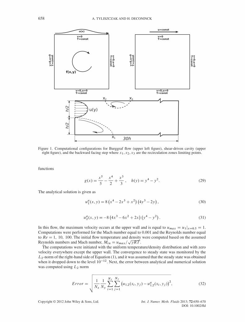
To demonstrate computational efficiency and accuracy of the proposed approach, we performedcomputations in three test cases shown schematically in Figure 1. The chosen flow problems include(i) a modified shear-driven cavity flow—the so-called Burggraf flow; (ii) a classical shear-drivencavity flow (2D and 3D configurations); and (iii) flow over a backward facing step. Although allthese configurations are typical test cases for the incompressible flows, they are also valid in otherMach number regimes. The absence of compressibility effects forM << 1 allowed for comparisonsof the obtained solutions with the results for the incompressible flows taken from a literature.

5.1. Modified shear-driven cavity flow—Burggraf flow [27]

This test case is one of the few flow problems for which an analytical solution exists. Therefore, itis often used as a reference solution, see [28–30] for instance, as it allows for detailed assessmentof discretization accuracy. In this subsection, the attention was exclusively devoted to the accuracyissue of the applied compact discretization method and therefore, we did not concentrate on the effi-ciency of the preconditioned and unpreconditioned solutions. This aspect is extensively analyzed inthe next subsections.

The computational domain is defined as a rectangular box Lx D Ly D 1.0. The flow insidethe cavity is induced by a forcing term and a motion of the upper wall with the horizontal veloc-ity defined as u1.x/ D 16

�x4 � 2x3C x2

�. The remaining walls are motionless, the temperature

of the walls is assumed constant, and the walls are treated as non-reflecting. The forcing term inEquation (1) for the vertical velocity component is defined as

fu2 D�

²8

Re

�24gC 2g00h00C g4h

� 64

�g02

2

�hh000 � h0h00

�� hh0

�g0g000 � g002

��³, (28)

where Re is the Reynolds number defined based on the height of cavity, Ly , and the maximumvelocity of the upper wall. The symbols g0,g00,g000,g.4/, h0, h00, h000 stand for the derivatives of the



Figure 1. Computational configurations for Burggraf flow (upper left figure), shear-driven cavity (upperright figure), and the backward facing step where x1, x2, x3 are the recirculation zones limiting points.

functions

g.x/Dx5

5�x4

2Cx3

3, h.y/D y4 � y2. (29)

The analytical solution is given as

ua1.x,y/D 8�x4 � 2x3C x2

� �4y3 � 2y

�, (30)

ua2.x,y/D�8�4x3 � 6x2C 2x

� �y4 � y2

�. (31)

In this flow, the maximum velocity occurs at the upper wall and is equal to umax D u1jxD0.5 D 1.Computations were performed for the Mach number equal to 0.001 and the Reynolds number equalto Re D 1, 10, 100. The initial flow temperature and density were computed based on the assumedReynolds numbers and Mach number, Min D umax=

p�RT .

The computations were initiated with the uniform temperature/density distribution and with zerovelocity everywhere except the upper wall. The convergence to steady state was monitored by theL2-norm of the right-hand side of Equation (1), and it was assumed that the steady state was obtainedwhen it dropped down to the level 10�12. Next, the error between analytical and numerical solutionwas computed using L2 norm

Error D

vuuut 1

Nx

1

Ny

NxXiD1

NyXjD1

�u1,2.xi ,yj /� ua1,2.xi ,yj /

�2, (32)



where Nx , Ny are the numbers of uniformly distributed mesh nodes. The same number of nodesin both directions was applied. Having solutions on a few meshes, the order of approximation wascomputed from

Order of appr.Dlog.Errorn=ErrornC1/

log.2/, (33)

where the subscripts refer to two consecutive meshes. Sample results obtained on the mesh 129�129nodes for Re D 100 are shown in Figure 2 which presents the contours of the velocity components,pressure, and the streamlines together with the velocity vectors showing the flow direction. Firstly,one may observe that all solutions are smooth and there are no sawtooth contours sometimesobserved in incompressible flow calculations when the pressure is not coupled correctly with thevelocity. Secondly, despite the fact that the amplitude of the pressure fluctuations is very low, lessthan 10�6, its changes are very well captured and there are no pressure oscillations nor strange,sharp profiles or discontinuities. The contours presented in Figure 2 are the first signs of the correct-ness of the algorithm and this is further confirmed in Tables I and II showing the solution errors andan estimated order of the approximation computed according to Equations (32) and (33), respec-tively. Here, we can see that for all the cases, the solution error decreases when the number of nodesincreases. In the same time, the order of approximation asymptotically approaches constant value,consistently with the expected fourth-order scheme.

0.0 0.2 0.4 0.6 0.8 1.00.0

0.2

0.4

0.6

0.8

1.0

0.0 0.2 0.4 0.6 0.8 1.00.0

0.2

0.4

0.6

0.8

1.0

0.0 0.2 0.4 0.6 0.8 1.00.0

0.2

0.4

0.6

0.8

1.0

0.0 0.2 0.4 0.6 0.8 1.00.0

0.2

0.4

0.6

0.8

1.0

Figure 2. Burggraf flow: velocity contours for u-component (left up figure) and v-component (right upfigure). Pressure contours (left down figure), streamlines, and velocity vectors (right down figure).



Table I. Grid refinement study for modified driven cavity flow for u1 velocity component.

Re D 1 Re D 10 Re D 100

Grid Error Order Error Order Error Order

17� 17 5.83� 10�4 — 6.14� 10�4 — 6.69� 10�3 —33� 33 5.82� 10�5 3.32 6.10� 10�5 3.33 6.24� 10�4 3.4265� 65 3.91� 10�6 3.89 4.08� 10�6 3.90 4.08� 10�5 3.93129� 129 2.29� 10�7 4.09 2.37� 10�7 4.10 2.35� 10�6 4.11257� 257 1.39� 10�8 4.04 1.34� 10�8 4.14 1.37� 10�7 4.09

Table II. Grid refinement study for modified driven cavity flow, for u2 velocity component.

Re D 1 Re D 10 Re D 100

Grid Error Order Error Order Error Order

17� 17 3.03� 10�4 — 3.89� 10�4 — 7.55� 10�3 —33� 33 3.32� 10�5 3.24 3.85� 10�5 3.33 6.90� 10�4 3.4565� 65 2.30� 10�6 3.79 2.67� 10�6 3.84 4.52� 10�5 3.93129� 129 1.40� 10�7 4.03 1.56� 10�7 4.09 2.61� 10�6 4.11257� 257 8.47� 10�9 4.05 9.50� 10�9 4.04 1.50� 10�7 4.12

Iteration number0 100 200 300 400 500 600 x 103-7

-6

-5

-4

-3

-2

-1

0

1

2

3

Re=300 (no prec.)

Re=300

Re=500 (no prec.)

Re=500Re=700

Re=700 (no prec.)

Iteration number0 100 200 300 400 500 600 x 103-7

-6

-5

-4

-3

-2

-1

0

1

2

3

Re=300 (no prec.)

Re=300

Re=500 (no prec.)

Re=500

Re=700

Re=700 (no prec.)

Log 1

0(L 2

-nor

m)

drop

Log 1

0(L 2

-nor

m)

drop

Figure 3. Backward facing step: convergence history for computations with the inlet Mach number Min D0.1 (left figure) and Min D 0.01 (right figure) for Reynolds numbers Re D 300, 500, 700.

5.2. Backward facing step

Flow over a backward facing step is another test case frequently used in computations of the incom-pressible flow. Here, we used the 2D configuration applied in [29, 31, 32] among others. The lengthof the channel is equal to 30h where the symbol h stands for the height of the channel whichis equal to twice the step height (see Figure 1). The Reynolds number is defined based on theheight of the channel and the maximum velocity at the inlet plane where the velocity profile isdefined as u1 D 12y.1 � 2y/, u2 D 0 and the temperature is constant. The temperature of thewalls is assumed constant as well, and the walls are motionless and treated as non-reflecting. Theoutflow condition is assumed as subsonic and non-reflecting. The numerical mesh was the sameas in [29] and it consisted of 301 � 101 uniformly distributed nodes. The computations were per-formed for the inlet Mach numbers Min D 0.1 and Min D 0.01 and for the Reynolds numbersRe D 100� 700. In all the cases, the initial temperature corresponded to the wall temperature andthe initial velocity was equal to zero. The convergence history for computations with and with-out application of the preconditioning is shown in Figure 3 where the lines represent a drop in



0 5 10-0.5

-0.25

0

0.25

0.5Re = 100

0 5 10-0.5

-0.25

0

0.25

0.5Re = 300

0 5 10-0.5

-0.25

0

0.25

0.5Re = 500

0 5 10-0.5

-0.25

0

0.25

0.5Re = 700

Figure 4. Backward facing step: contours of the u-velocity component for M D 0.01 and Re D100, 300, 500, 700.

L2-norm of the right-hand side of Equation (1). The computations were stopped when the L2-normdropped six orders of magnitude with respect to the initial value or when the number of iterationsexceeded 6� 105.

Let us first discuss the unpreconditioned solution for the case with Min D 0.1. The convergencerate is very poor and the residual does not reach the assumed level, although the solution is stableand the residual decreases. One may hope that it would converge if the computations were continuedfor a very long time. The situation is different in the case of Min D 0.01; here, we can see that forthe higher Reynolds numbers, the solutions diverge. For Re D 300, the solution is stable but itsconvergence rate is extremely low, in fact, it is much worse than for Min D 0.1. Such behavior isattributed to the following reasons: (i) the errors related to the convective terms are not effectivelytransported out of the system; (ii) variations of the density and pressure fields are so tiny that theircomputations become contaminated by the numerical errors; and (iii) these errors accumulate in thesubsequent iterations and if not damped by the natural or artificial viscous dissipative terms, theylead to instability. We note that reduction of the time step does not help to stabilize the solution andit only postpones the time when the solution starts to diverge.

The convergence of the solution with preconditioning is significantly better than without thepreconditioning. One may notice that the preconditioned solutions are mainly dependent on theReynolds number and very little on the Mach number. Thanks to that, the solution converges evenfor Mach numbers smaller than 0.01, as it will be presented in the next sections.

The measure of the correctness of the solution for the backward facing step are the positionand length of the recirculation zones appearing just behind the step and also on the upper wall (inthe case of higher Reynolds number). Figure 4 shows contours of the u-velocity component in thesolutions obtained for Min D 0.01 and for various Re. Here, we can see that in all the cases, thelength of the lower recirculation zone increases with the Reynolds number. The upper recirculationzone is seen only for Re D 500 and Re D 700; here, one may observe that both the separationpoint, X2, and the reattachment point, X3, move downstream when the Reynolds number increases.Comparison of the reattachment and separation points with experimental [31] and numerical [29]data is shown in Figure 5. In the cited works, the incompressible flow was analyzed; in [29], thenumerical algorithm was based on artificial compressibility approach, and the discretization was per-formed with the third-order upwind flux-difference splitting method. The results obtained presentlyshow that both the lower reattachment point, X1, as well as the position of the upper recirculationzones are predicted correctly and slightly better than in [29]—this may be attributed to the formallyhigher order of the approximation applied in the present computations. The position of the separa-tion point differs from the experimental data and as pointed in [29], this is probably due to possible3D effects in the experiment.



Reynolds number

Reynolds number

x/(h

/2)

x/(h

/2)

0 100 200 300 400 500 600 7002

4

6

8

10

12

14

Num. present resultsNum. Shah and Yuan (2009)Exp. Armaly et al. (1983)

x1

300 400 500 600 7006

7

8

9

10

11

12

13

14


x2

x/(h

/2)

300 400 500 600 7008

10

12

14

16

18

20

22


x3

Figure 5. Backward facing step: position of the lower (X1) and upper (X3) reattachment points and theposition of the separation point (X2) of the upper recirculation zone.

5.3. 2D classical shear-driven cavity flow

This test case is one of the best documented in literature, especially for the 2D case for whichdata from Ghia et al. [33] or Botella and Peyret [34] are usually taken as the reference solution.The geometry of the computational domain is exactly the same as used previously for the Burggrafflow. The only differences are the following: the velocity of the upper wall is assumed constant,u1 D 1, and there is no forcing term. For this test case, we performed a series of computationsfor various Reynolds numbers and also for a wide range of Mach numbers in order to demon-strate the excellent properties of the preconditioning. Hence, the computations were carried out forRe D 100, 400, 1000 and for Min D 0.5, 0.1, 0.01, 0.001. The results obtained for Min D 0.001are then compared with the literature data for the incompressible flow. The numerical meshes con-sisted of 128 � 128 and 256 � 256 uniformly distributed cells. In all the cases, the solution wasinitialized with zero velocity and uniform temperature. The convergence rate was again monitoredby the L2-norm of the right-hand side of Equation (1), the computations were stopped when theL2-norm dropped 10 orders of magnitude or the number of iterations reached the value 3�105. Theconvergence histories for the mesh 128 � 128 cells are presented in Figure 6, and we note that forthe mesh with 256�256 cells, the convergence histories look similarly, although the number of iter-ations needed to reach the assumed reduction of the residual is larger. Analyzing Figure 6, a generalobservation is that the number of iterations necessary to converge increases when the Mach numberdecreases or when the Reynolds number increases. We can see that in the case of relatively highMach number, that is, Min D 0.5, the convergence rate is similar regardless whether the precondi-tioning was applied or not. Indeed, for Re D 100, the unpreconditioned solution converges slightlyfaster comparing with the preconditioned one. The situation changes evidently when the Mach num-ber decreases; in this case, the convergence rate of the unpreconditioned solutions is either very pooror the solutions are unstable and diverge shortly after the solution procedure starts. Unlike to that



Iteration number0 50 100 150 200 250 300 x 103




-10

-8

-6

-4

-2

0

2

4

Re = 100 (no prec.)Re = 400 (no prec.)Re = 1000 (no prec.)Re = 100Re = 400Re = 1000

Min = 0.5 Re = 100 (no prec.)Re = 400 (no prec.)Re = 1000 (no prec.)Re = 100Re = 400Re = 1000

Min = 0.1


Min = 0.01 Re = 100 (no prec.)Re = 400 (no prec.)Re = 1000 (no prec.)Re = 100Re = 400Re = 1000

Min = 0.001

Log 1

0(L 2

-no

rm)

drop

-10

-8

-6

-4

-2

0

2

4

Log 1

0(L 2

-no

rm)

drop

-10

-8

-6

-4

-2

0

2

4

Log 1

0(L 2

-no

rm)

drop

-10

-8

-6

-4

-2

0

2

4

Log 1

0(L 2

-no

rm)

drop

Figure 6. 2D driven cavity flow: convergence history for computations with the inlet Mach numberMin D 0.5, 0.1, 0.01 and Min D 0.001 for Reynolds numbers Re D 100, 400, 1000. Solutions without

the application of preconditioning are represented by the lines without symbols.

behavior, the convergence rate of the preconditioned solution is very good for all analyzed casesand it seems to be very little dependent on the Mach number. Although, for Min D 0.001, when theresidual dropped approximately, nine orders of magnitude, we may see that it stagnates at the levelapproximately equal to 10�12. This is comparable with the level of machine precision, and thusthe round-off error may become an important factor influencing the solution and holding the totalerror at the constant level. Nevertheless, we assumed that the obtained solution for Min D 0.001was fully converged and we could start to compare it with the literature data from Ghia et al. [33]and other more recent solutions. First of all, in Figure 7 as in many other papers, we present thecontours of the pressure, vorticity, and the stream-function. Additionally, because we deal with acompressible solver, the contours of the Mach number are also shown. The solution exhibits twosmaller vortices located in the corners and a large primary vortex in the center. The values and posi-tion of the maximum of the stream-function in the primary vortex is one of the main parametersused to verify the solution. Detailed results are given in Table III together with the reference solu-tions from [35, 36] obtained with the third-order schemes. We can see in this table that the presentresults compare very well with the literature data on both meshes. Furthermore, if we compare thepresent values of the stream-function and vorticity with the results obtained on a very fine mesh.1024 � 1024/, we may see that they agree slightly better than the corresponding literature data.Finally, in Figure 8, we compare the velocity profiles along the cavity main axes, the u1-componentof velocity along y-axis, and u2-component of velocity along x-axis. These results were obtained



0.0 0.2 0.4 0.6 0.8 1.00.0

0.2

0.4

0.6

0.8

1.0

0.0 0.2 0.4 0.6 0.8 1.0

0.0 0.2 0.4 0.6 0.8 1.0

0.0

0.2

0.4

0.6

0.8

1.0

0.0

0.2

0.4

0.6

0.8

1.0

0.0 0.2 0.4 0.6 0.8 1.00.0

0.2

0.4

0.6

0.8

1.0

Figure 7. 2D driven cavity flow: contours of the pressure (upper-left figure), vorticity (upper-rightfigure), the Mach number (lower left figure) and the stream-function (lower-right figure) for M D 0.001

and Re D 1000.

Table III. Comparison of the present and reference solutions for M D 0.001and Re D 1000. Maximum value of the stream-function of the primary vortex,

corresponding vorticity, and location.

Solution Grid max ! x - position y - position

Present 128� 128 0.11806 2.0544 0.53125 0.56250Bruneau et al. [35] 128� 128 0.11786 2.0508 0.53125 0.56250Kawamura et al. [36] 128� 128 0.11790 2.0557 0.53125 0.56250

Present 256� 256 0.11873 2.0653 0.53125 0.56640Bruneau et al. [35] 256� 256 0.11865 2.0634 0.53125 0.56640Kawamura et al. [36] 256� 256 0.11867 2.0636 0.53125 0.56640

Bruneau et al. [35] 1024� 1024 0.11892 2.0674 0.53125 0.56543Kawamura et al. [36] 1024� 1024 0.11892 2.0674 0.53125 0.56445

on the mesh 128 � 128 cells, we note that the results on the finer mesh are hardly distinguishable.As the reference solution, we added the results from [33] represented by the symbols, and as onemay see, the present solutions agree very well with [33] for both velocity components and for allReynolds numbers (see Figure 8).



Figure 8. 2D driven cavity flow: profiles of the horizontal .u1/ and vertical .u2/ velocity along x and yaxes of the cavity for M D 0.001 and Re D 100, 400, 1000.

x

00.2

0.40.6

0.81

z

00.2

0.40.6

0.81

y

0

0.2

0.4

0.6

0.8

1

y

x z

z

y

0 0.2 0.4 0.6 0.8 10

0.2

0.4

0.6

0.8

1

Figure 9. 3D driven cavity flow with M D 0.001 and Re D 1000. Left figure: isosurfaces of the u3—velocity component (green color u3 D 0.035, red color u3 D �0.035). Right figure: streamlines with the

velocity vectors in the y � ´ plane at x D 0.5.

5.4. 3D shear-driven cavity flow

The nature and configuration of the flow in 3D shear-driven cavity is very similar to the 2D case. Weconsider a 3D cavity where all the walls have constant temperature and except for the upper wall, allthe others are motionless. The upper wall moves with the constant horizontal velocity u1 D 1. Thegoal of these computations was to demonstrate the efficiency and accuracy of the present approachin 3D flow problem.

The computations were performed for the Reynolds number equal to Re D 100, 400, 1000 andthe Mach number equal to M D 0.1 and M D 0.001. In the latter case, the results were com-pared with the data from Ku et al. [37]. We used two uniformly spaced meshes with 63 � 33 � 63and 93 � 65 � 93 nodes in x, ´,y directions, respectively. Sample results presenting the 3D flowstructures are shown in Figure 9 where the presented isosurfaces correspond to constant values ofthe z-velocity component equal to u3 D ˙0.035 (red color corresponds to negative value). Addi-tionally, the stream-traces together with the vector field in the cross-section plane .y � ´, x D 0.5/are also presented in Figure 9 on the right-hand side. Here, the symmetry of the flow is readilyseen, and the flow exhibits four counter-rotating vortices located in the corners. The convergence



Iteration number Iteration number0 50 100 150 200 250 300 x 103

-10

-8

-6

-4

-2

0

2

4


Min = 0.1

0 20 40 60 80 100 x 103


Min = 0.001

Log 1

0(L 2

-no

rm)

drop

-10

-8

-6

-4

-2

0

2

4

Log 1

0(L 2

-no

rm)

drop

Figure 10. 3D driven cavity flow: convergence history for computations on the coarse mesh (63 �33 � 63 nodes) for the inlet Mach number Min D 0.1 and Min D 0.001 for the Reynolds numbersRe D 100, 400, 1000. Solutions without the application of preconditioning are represented by the lines

without symbols.

Y-c

oord

inat

e

-0.4 -0.2 0 0.2 0.4 0.6 0.8 10

0.2

0.4

0.6

0.8

1

PresentPresentPresent(coarse mesh)

a.b.c.

Re = 100Re = 400Re = 1000

Ku et al. (1987)Re = 100Re = 400Re = 1000

b.

a.

c.

Present

X-coordinate0 0.2 0.4 0.6 0.8 1

-0.4

-0.2

0

0.2

PresentPresentPresent

(coarse mesh)a.b.c.

Re = 100Re = 400Re = 1000

Ku et al. (1987)

Re = 100Re = 400Re = 1000

b.

a.

c.

Present

u1- velocity

u 2-ve

loci

ty

Figure 11. 3D driven cavity flow: profiles of the horizontal .u1/ and vertical .u2/ velocity along x and yaxes of the cavity for M D 0.001 and Re D 100, 400, 1000.

history for computations on the coarse mesh is shown in Figure 10 where the lines with symbolscorrespond to the solutions with the preconditioning. Similarly as in 2D cases, the benefits fromits application are evident. First of all, it significantly accelerates the convergence, and moreoverin low Mach number conditions, it stabilizes the solution. In the computations for Min D 0.001,the unpreconditioned solutions diverge, whereas in the computations involving preconditioning, theerror is quickly reduced by approximately eight orders of magnitude.

Finally, the correctness of the results is confirmed in Figure 11 by comparison with the literaturedata from Ku et al. [37]. In [37], the Chebyshev pseudospectral method was used with 25� 45� 25and 31� 61� 31 modes for Re D 100, 400 and Re D 1000, respectively. Applying the Chebyshevapproximation by definition compacts the numerical nodes close to the boundaries what certainlyincreases the accuracy. Analyzing the results in Figure 11, one may notice that the agreement is notas good as in 2D configurations, particularly for Re D 1000. In the case of Re D 100, the resultsare very good and almost independent of the mesh. The biggest influence of the number of nodesis observed for Re D 1000, where one may see that increasing the number of nodes improves thesolution. Therefore, referring to the excellent agreement in the 2D cases, one should keep in mind



that in 3D computations, the numerical mesh was coarser than in 2D, and this may be the mainreason of the observed small discrepancies. Nevertheless, the presented solutions are very close tothe reference ones.

6. CONCLUSIONS

In this paper, the preconditioning method has been used in the computations of flow problems atmoderate and very low Mach number regimes. The procedure of imposing the BCs by the NSCBCapproach has been modified accordingly by including the reference Mach number in the boundaryscheme and taking into account the modified eigenvalues of the system. The spatial discretizationhas been performed by high-order compact method which together with the use of preconditioninghas led to a very accurate and efficient algorithm. This has been confirmed performing computationsin the typical benchmark cases for a wide range of Mach and Reynolds numbers. It was shown thatapplication of the preconditioning considerably speeds-up the convergence to the steady state andthe final steady solutions are consistent with the reference results. Furthermore, the solution of thepreconditioned system was always stable regardless how small the Mach number was, whereasthe solutions without preconditioning revealed unstable when the Mach number was small andthe Reynolds number was higher (Re D 400, 1000 in the case of cavity flow). Such behaviorof the solution was attributed to the fact that in the low Mach number conditions, the solutionsbecame considerably affected by the errors connected to the convective waves and probably alsothe numerical errors which were not transported efficiently out of the computational domain. Inthe successive iterations, this created high-frequency phenomena which were neither damped by thephysical dissipation nor properly resolved by the numerical scheme leading eventually to instability.In the case of low-order discretization or discretization combined with some stabilization method(upwind, Total Variation Diminishing (TVD), non-oscillatory schemes), there is a chance that thesolution would remain stable. This is however not the case for the compact schemes which havevery little amount of the numerical dissipation and therefore are prone to instability. Numerouscomputational examples presented in the paper showed that the application of preconditioningmakes the solution procedure resistant to the aforementioned errors. As explained in the paper,the application of preconditioning largely equalizes the convective and acoustic wave speeds andbecause of that, the solution errors are successfully removed from the domain. From this point ofview, an additional benefit of applying preconditioning in connection with high-order discretizationis evident because apart from the convergence acceleration, it also stabilizes the computations atvery low Mach number regimes.

APPENDIX A

Locally, 1D inviscid flow defined in Equation (8) is given as

@Qp

@tC �p

@F1

@x1D 0, (A.1)

where the matrix �p is defined as

�p D

0BBBB@

12jEuj2‚0 �u1‚

0 �u2‚0 �u3‚

0 ‚0

�u1=� 1=� 0 0 0

�u2=� 0 1=� 0 0

�u3=� 0 0 1=� 012jEuj2‚00 � T=� �u1‚

00 �u2‚00 �u3‚

00 ‚00

1CCCCA , (A.2)

where jEuj is the modulus of the velocity vector and the parameters ‚0 and ‚00 are defined as

‚0 DM 2r .� � 1/ , ‚00 D

‚0C 1

�Cp. (A.3)



The system (A.1) may be transformed to

@Qp

@tC �pA„ƒ‚…

R�L

@Qp

@x1D 0, (A.4)

whereRD L�1 are the right and left eigenvector matrices andƒ is the diagonal matrix of the eigen-values of the product of the �p matrix and the transformation matrix A D @F1

@Qp. Transformation of

(A.4) to the characteristic form leads to

L@Qp

@tCƒL

@Qp

@x1D 0,

@ OQp

@tCƒ

@ OQp

@x1D 0,

(A.5)

with the characteristic variables OQp D L@Qp expressed as

OQp D

0BBBB@@pC �

�� M

2r u1

�@u1

@T � @p=.�Cp/@u2@u3

@pC ��C �M

2r u1

�@u1

1CCCCA . (A.6)

Thus, the characteristic system may be explicitly written as

@p

@tC �

�� M

2r u1

� @u1@tC ��

�@p

@x1C �

�� M

2r u1

� @u1@x1

�„ ƒ‚ …

W1

D 0, (A.7)

@T

@t�

1

�Cp

@p

@tC u1

�@T

@x1�

1

�Cp

@p

@x1

�„ ƒ‚ …

W2

D 0, (A.8)

@u2

@tC u1

@u2

@x1„ƒ‚…W3

D 0 I@u3

@tC u1

@u3

@x1„ƒ‚…W4

D 0, (A.9)

@p

@tC �.�C �M

2r u1/

@u1

@tC �C

�@p

@x1C �.�C �M

2r u1/

@u1

@x1

�„ ƒ‚ …

W5

D 0, (A.10)

where the variables W1, W2, W3, W4, W5 introduced previously represent the time variations ofthe characteristic variables. Subtracting Equation (A.10) from Equation (A.7) results in

@u1

@tD

W1 �W5

�.�C � ��/, (A.11)

which then is introduced to Equation (A.7) that gives

@p

@tD

W5

�� M

2r u1

��W1

��C �M

2r u1

��C � ��

. (A.12)

Using the aforementioned expression in Equation (A.8) leads to

@T

@tD�W2C

1

�Cp

W5

�� M

2r u1

��W1

��C �M

2r u1

��C � ��

. (A.13)

Hence, the Equations (A.9), (A.11), (A.12), and (A.13) result in the system defined byEquations (9)–(13).



ACKNOWLEDGMENT

The first author has been supported by the statutory funds BS/PB-1-103-3010/2011/P. Part of the computa-tions have been performed using the PL-Grid infrastructure under grant LESCMC.

REFERENCES

1. Cook WC, Riley JJ. Direct numerical simulation of a turbulent reactive plume on a parallel computer. Journal ofComputational Physics 1996; 129:263–283.

2. Guillard H, Viozat C. On the behaviour of upwind schemes in the low Mach number limit. Computers and Fluids1999; 28:63–86.

3. Venkateswaran S, Merkle CL. Analysis of preconditioning methods for Euler and Navier–Stokes equations. In 30thComputational Fluid Dynamics Lecture Series. Von Karman Institute: Rhode-Saint-Genese, 1999.

4. Majda A, Sethian J. The derivation of the numerical solution of the equations for zero Mach number Combustion.Combustion Science & Technology 1985; 42:185–205.

5. Turkel E. Preconditioned methods for solving the incompressible and low speed compressible equations. Journal ofComputational Physics 1987; 72:277–298.

6. Lee D. Local preconditioning of the Euler and Navier-Stokes equations. Ph.D. Thesis, University of Michigan, 1996.7. Lee D. Design criteria for local Euler preconditioning. Journal of Computational Physics 1998; 144:423–459.8. Lee D. The design of local Navier–Stokes preconditioning for compressible flow. Journal of Computational Physics

1998; 144:460–483.9. van Leer B, Lee WT, Roe P. Characteristic time-stepping or local preconditioning of the Euler equations. AIAA

Paper, 1991. (91-1552).10. Turkel E. Preconditioning techniques in computational fluid dynamics. Annual Review of Fluid Mechanics 1999;

31:385–416.11. Venkateswaran S, Merkle CL. Dual time stepping and preconditioning for unsteady computations. AIAA Paper, 1995.

(1995-0078).12. Turkel E, Vatsa VN. Local preconditioners for steady state and dual time-stepping in mathematical modeling and

numerical analysis. ESAIM: Mathematical Modelling and Numerical Analysis 2005; 39:515–536.13. Lele SK. Compact finite difference with spectral-like resolution. Journal of Computational Physics 1992; 103:16–42.14. Carpenter MH, Gottlieb D, Abarbanel S. The stability of numerical boundary treatements for compact high-order

finite-difference schemes. Journal of Computational Physics 1993; 108:272–295.15. Carpenter MH, Gottlieb D, Abarbanel S. Time-stable boundary conditions for finite-difference schemes solving

hyperbolic systems: methodology and applications to high-order compact schemes. Journal of ComputationalPhysics 1994; 111:220–236.

16. Thompson KW. Time dependent boundary conditions for hyperbolic systems. Journal of Computational Physics1987; 68:1–24.

17. Poinsot TJ, Lele SK. Boundary conditions for direct simulations of compressible viscous flows. Journal ofComputational Physics 1992; 101:104–129.

18. Hejranfar K, Kamali-Moghadam R. Preconditioned characteristic boundary conditions for solution of the precondi-tioned Euler equations at low Mach number flows. Journal of Computational Physics 2012; 231:4384–4402.

19. Li HG, Zong N, Lu XY, Yang V. A consistent characteristic boundary condition for general fluid mixture and itsimplementation in a preconditioning scheme. Advances in Applied Mathematics and Mechanics 2012; 4:72–92.

20. Canuto C, Hussaini MY, Quarteroni A, Zang T. Spectral Methods in Fluid Dynamics. Springer-Verlag: BerlinHeidelberg, 1988.

21. Kennedy CA, Gruber A. Reduced aliasing formulations of the convective terms within the Navier–Stokes equationsfor compressible fluids. Journal of Computational Physics 2008; 227:1676–1700.

22. Santhanam N, Lele SK, Ferziger JH. A robust high-order compact method for large eddy simulation. Journal ofComputational Physics 2003; 191:392–419.

23. Vichnevetsky R, Bowles JB. Fourier Analysis of Numerical Approximations of Hyperbolic Equations. SIAM:Philadelphia, 1982.

24. Gustafsson B. The convergence rate for difference approximations to mixed initial boundary value problems.Mathematics of Computation 1975; 29:396–406.

25. Fletcher CAJ. Computational Techniques for Fluid Dynamics. Springer-Verlag: Berlin Heidelberg, 1991.26. Hirsh Ch. Numerical Computation of Internal and External Flows. John Wiley & Sons: Chichester, 1990.27. Burggraf OR. Analytical and numerical studies of the structure of steady separated flows. Journal of Fluid Mechanics

1966; 24:113–151.28. Pereira JMC, Kobayashi MH, Pereira JCF. A fourth-order-accurate finite volume compact method for the incom-

pressible Navier–Stokes solutions. Journal of Computational Physics 2001; 167:217–243.29. Shah A, Yuan L. Flux-difference splitting-based upwind compact schemes for the incompressible Navier–Stokes

equations. International Journal for Numerical Methods in Fluids 2009; 61:552–568.30. Laizet S, Lamballais E. High-order compact schemes for incompressible flows: a simple and efficient method with

quasi-spectral accuracy. Journal of Computational Physics 2009; 228:5989–6015.



31. Armaly BF, Durst F, Pereira JCF, Schonung B. Experimental and theoretical investigation of backward facing stepflow. Journal of Fluid Dynamics 1983; 172:473–496.

32. Kim J, Moin P. Application of a fractional step method to incompressible Navier–Stokes equations. Journal ofComputational Physics 1985; 59:308–323.

33. Ghia U, Ghia KN, Shin CT. High-Re solutions for incompressible flow using the Navier–Stokes equations and amultigrid method. Journal of Computational Physics 1982; 48:387–411.

34. Botella O, Peyret R. Benchmark spectral results on the lid-driven cavity flow. Computers and Fluids 1998;27:421–433.

35. Bruneau C-H, Saad M. The 2D lid-driven cavity problem revisited. Computers and Fluids 2006; 35:326–348.36. Kawamura T, Takami H, Kuwahara K. New higher-order upwind scheme for incompressible Navier–Stokes

equations. Lecture Notes in Physics 1985; 218:291–295.37. Ku HC, Hirsh RS, Taylor TD. A pseudospectral method for solution of the three-dimensional incompressible

Navier–Stokes equations. Journal of Computational Physics 1987; 70:439–462.


application of time preconditioning and high-order compact discretization method for low mach number...

Documents