Application of Particle Filtering for Sequential Inferences of StochasticVolatility Modeled with Leverage

Mahsiul Khana,1,2,∗, Richard V. Rothenbergb,3,

aQuantum Filtering Algorithm LLC, NY, USAbGlobal Algorithmic Institute, NYC, USA

Abstract

In this article, we implement the Particle Filtering (PF) algorithm for sequential inferences of the stochasticvolatility (SV) modeled with leverage. Our implementationand applications are based on the recent work byDjuric et al. (2012) and the earlier work by Khan (2011) and Liu and West (2001). The standard SV modelsis a dynamic state space models where the underlying volatility process is assumed an autoregressive hiddenprocess, and the innovations of the state and observed processes are assumed independent and Gaussianwhite noises with zero mean and unit variance. But, the paperby Djuric et al. (2012) modeled the noiseprocesses as correlated, and called it modeled with leverage. The paper also applied Rao-Blackwellization(RB) method, a variance reduction technique which integrate out the static and nuissance parameters, whichreduces the dimension of unknowns and computational complexities. The RB method shows advantage onconvergence with the smaller particle size, and improve estimates by reducing the variance of unknowns.The objective is to get real-time inferences of the underlying volatility (log-volatility) as the observationsarise sequentially in time.

Keywords: Particle filtering, stochastic volatility, Bayesian, dynamic state space, leverage.

1. Introduction

The increasing number of interlinkages and interdependencies in the global financial system have ledto an augmented potential for cascading failure and financial crisis contagion, as evidenced in the failure ofLTCM in 1998 and the subprime mortgage crisis in 2008. These events have demonstrated the compellingneed for policymakers, regulators and financial industry participants to develop new methods and state-of-the-art tools to better understand, monitor and mitigate global systemic risk. Managing Financial Riskhas been an important aspects of the corporations, financialinstitutions and global central banks, wherevolatility is one of the key metric to manage and model risk. One of the main focus of our research is

∗Corresponding authorEmail addresses:mahsiul.khan@gmail.com (Mahsiul Khan),richard.v.rothenberg@gmail.com (Richard V.

Rothenberg)1Dr. Mahsiul Khan is a Researcher at the Global Algorithmic Institute, NYC.2Dr. Mahsiul Khan is a founder of Quantum Filtering AlgorithmLLC, NY.3Richard V. Rothenberg is a Researcher at the Global Algorithmic Institute, NYC.

Preprint submitted to Elsevier February 8, 2015

to model and measure/predict the risk poses on the global financial systems due to increasing electronictrading especially HFT (high frequency trading). The exactsources of the volatility is not known, but,the various factors such as economical, financial, geo-political, natural events, trading volume as well asirrational behaviors of market participants are assumed tocreate uncertainty in the markets. We applyPF algorithm on SV model since SV is a dynamic predictive model, and can be used to predict/asses thevolatility/risk dynamically. The volatility is a measure ofMarket Risk, therefore, modeling and estimatingvolatility are in great demand among practitioners and academics.

2. Modeling Volatility

In statistics, volatility is defined as the standard deviation (σt) of asset price. Study suggest that thevariance of time seriesσ2

t , is heteroscedastici.e., it changes over time. Hence, it is modeled as a non-stationary process.

rt = µ + σtvt (1)

yt = σtvt (2)

yt ∼ N(0, σ2t ) (3)

σ2t = α0 + α1y2

t−1, ARCH(1) (4)

σ2t = α0 + α1y2

t−1 + β1σ2t−1, GARCH(1, 1) (5)

wherert = (Pt/Pt−1 − 1) is standard return series,Pt is price,µ is expected return,yt = rt − µ is mean sub-tracted return series, andvt is standard Gaussian noise process, i.e.vt ∼ N(0, 1). The two most widely usedvolatility models, ARCH (auto regressive conditional heteroscedasticity) and GARCH( generalized auto re-gressive conditional heteroscedasticity) are developed by Engle (1982) and Bollerslev (1986) respectivelyto model the volatility.

3. Standard SV Models-Uncorrelated Noise Processes

An alternative hypothesis is that the volatility is a hidden/underlying process, which is not observeddirectly from the return series. Hence, the formation of theSV models developed by Rosenberg (1972),Clark (1973), Black and Scholes (1972), Taylor (1982), Taylor (2005), Ghysels et al. (1996) and Shephard(1996) as a discrete time dynamic state-space (DSS) models,a class of HMM is considered. The standardSV model is defined as,

xt = β1 + β2xt−1 + σuut (state equation) (6)

yt = ext/2vt (observation equation) (7)

wherext = log(σ2t ), xt ∈ R is log-volatility, ut and vt are independent and identically distributed stan-

dard Gaussian noise process, i.e.,ut, vt ∼ N(0, 1), andβ1, β2, andσu are unknown static but nuissanceparameters. Objective is to get sequential inferences ofxt asyt is observed dynamically in time.

2

4. Leverage SV Models-Correlated Noise Processes

It has been observed that there is a negative correlation between volatility and return series, and mod-eling this phenomena is called Leverage SV models (Black, 1976; Nelson, 1991; Jacquier et al., 2004; yu,2005; Djuric et al., 2012). When the prices decrease dramatically and the returns are negative, the volatilityspikes, as seen in 2008-2009 during the market crash when theVIX reached all time high. Hence, the SVmodels with correlated noise processes/shocks of state and observations are defined as,

ut = ρvt−1 +

√1− ρ2u′t (8)

xt = β1 + β2xt−1 + σuρvt−1 + σu

√1− ρ2u′t

= β1 + β2xt−1 + β3yt−1e−xt−1

2 + ζu′t (state) (9)

yt = ext/2vt (observation) (10)

wherecorr(ut, vt−1) = ρ, β3 = σuρ, ζ = σu

√1− ρ2 andu′t is another standard Gaussian noise process,

independent ofvt−1 andut. The unknown parameter vectorθ = [β1 β2 σu ρ]. We observe that in thisleverage models,xt has autocorrelation withxt−1 andyt−1, which has more intuitive explanation.

5. Rao-Blackwellization(RB)

The RB method transforms an ordinary estimator into an improved estimator based on Rao-Blackwelltheorem (Lehmann, 1991). It reduces the variance of the estimate based on mean-squared error (MSE)criterion. The RB (Casella and Robert, 1996; Doucet et al., 2000) also refers to dimensionality reductionin unknown space, such as state space in DSS models. Due to thepresence of unknown static parametersθ = [β1 β2 σu ρ]⊤, the full joint posterior PDF has the form asp(xt, θ|x0:t−1, y1:t−1). Hence, it requires MCsampling from joint posterior, i.e, from state and parameter spaces respectively. Since the parameters arenuisance, if one can integrate out the parameter vectorθ, the resultant distribution is the desired filteringPDF p(xt|x0:t−1, y1:t−1), which marginalizes the joint posterior PDF by reducing total sampling space. Con-sequently, this reduction in dimension reduces the variance of the estimate and improves accuracy. Thisprocess is also called RB.

p(xt|x0:t−1, y1:t−1) =

∫

θ

p(xt, θ|x0:t−1, y1:t−1)dθ

=

∫

θ

p(xt|θ, x0:t−1, y1:t−1)p(θ|x0:t−1, y1:t−1)dθ

∝ tν(m, r) (11)

wheretν(m, r) is non-standard t-PDF withν degrees of freedom (df), m=mean and r=variance. We marginal-ize parameter space by using implied integration method, and hence the marginal filtering PDF becomesnon-standard t-PDF as described above.

3

6. Particle Filtering- A Sequential Bayesian Filtering

Particle Filtering (PF) or Sequential Monte Carlo (SMC) is asimulation based methods based on Bayes’theorem (Gordon et al., 1993; Doucet et al., 2001, 2000; Arulampalam et al., 2002; Maskell, 2004; Djuricet al., 2003; Djuric and Bugallo, 2009). When the DSS systemsare linear and Gaussian, the Kalmanfilter (Kalman, 1960) is the optimal solution. But, most realworld dynamical systems are non-linear andnon-Gaussian, and obtaining sequential inferences of their hidden states has been a challenge. Variousextensions of Kalman filter such as extended Kalman filter (Anderson and Moore, 1979) and Gaussian sumfilter (Sorenson and Alspach, 1971) are also being used for non-linear systems. But, when non-linearity istoo high these methods perform poorly. For non-linear and/or non-Gaussian systems, the PF has superiorperformance over existing methods according to research and literatures. PF has wide range of applicationsin science and engineering, including statistical signal processing, target tracking, missile guidance, terrainnavigation, neural networks, financial modeling, and time series analysis and forecasting. Many real worldproblem such as in finance, where observations arrive sequentially in time and objective is to get realtimeinferences of the unknown state. The PF under Bayesian methodology provides sequential inferences ofposterior PDF as observation arrives in time.

6.1. Bayesian InferencesLet x0:t ≡ (x0, ..., xt) andy1:t ≡ (y1, ..., yt) are defined as state and observation sequences respectively.

We assume that we have some prior knowledge about the unknowns, and all information of the unknownsare available in the posterior PDF. Hence, our objective is to sequentially estimate/predict the posterior PDF(Box and Tiao, 1992; Doucet et al., 2001). The transition from the prior to the posterior PDF defined as,

p(x0:t|y1:t,Ψ)︸ ︷︷ ︸posterior

=

likelihood︷ ︸︸ ︷p(y1:t |x0:t,Ψ)

prior︷ ︸︸ ︷p(x0:t |Ψ)

p(y1:t |Ψ)︸ ︷︷ ︸evidence

(12)

whereΨ is the assumed model.The posterior PDFp(x0:t|y1:t) and its various features are the main interest in Bayesian Inference. In

many applications, when the interest is on sequential estimation of posterior PDF, and often a particularinterest on its marginal the so calledfiltering PDF, p(xt|y1:t). The joint posterior PDF can be expressedrecursively as,

p(x0:t|y1:t) = p(x0:t−1|y1:t−1)p(yt|xt)p(xt|x0:t−1, y1:t−1)

p(yt|y1:t−1)(13)

One of the central idea in PF is to represent the posterior PDFby arandom measure, a set of weightedsamples, also known asparticles. These weighted particles approximate the posterior PDFp(x0:t|y1:t), bythe random measure,χ0:t = {xi

0:t,wit}

Ni=1, where{xi

0:t}Ni=1 are the set of support points with associated weights

{wit}

Ni=1, and{xi

0:t}Ni=1 are the possible trajectories/realizations of the state up to time instantt. As the number

of particles tends to infinity, the random measure, under given some conditions, tends almost surely to thetrue posterior PDF (Crisan and Doucet, 2002). Mathematically, we express

p(x0:t|y1:t) ≈

N∑

i=1

witδ(x0:t − xi

0:t) (14)

{xi0:t,w

it}

Ni=1

a.s−→ p(x0:t|y1:t) as N→ ∞ (15)

4

whereδ(·) is theDirac deltafunction. These weighted particles constitute the discrete approximation of thetrue posterior PDF. The weights are computed by using the principle ofimportance sampling (IS)(Geweke,1989). The particles/samples are generated from theimportance function q(x0:t |y1:t) such thatsupp(q) ⊃supp(p), wherep(·) is the generic target posterior PDF. If the importance function can be factorized as,

q(x0:t|y1:t) = q(x0:t−1|y1:t−1)︸ ︷︷ ︸keep existing path

q(xt|x0:t−1, y1:t)︸ ︷︷ ︸extend path

(16)

then it is possible to obtain samples (trajectories)xi0:t ∼ q(x0:t |y1:t) up to timet, by augmenting the existing

trajectoriesxi0:t−1 ∼ q(x0:t−1|y1:t−1) with the current state samplesxi

t ∼ q(xt|x0:t−1, y1:t) at timet. Thus, therecursive importance function allows us to express the weight update equation as,

wit ∝

p(xi0:t |y1:t)

q(xi0:t |y1:t)

∝ wit−1

p(yt|xit)p(xi

t |xi0:t−1, y1:t−1)

q(xit|x

i0:t−1, y1:t)

(17)

If we sample from the marginal filtering PDFp(xit|x

i0:t−1, y1:t−1), thenq(xi

t |xi0:t−1, y1:t) = p(xi

t |xi0:t−1, y1:t−1),

and consequently our updated weight equation becomes,

wit ∝ wi

t−1p(yt|xit) (18)

6.2. A Generic PF Algorithm

This algorithm is based on choosing prior distribution as importance function, i.e.,q(xt|xt−1, yt) =p(xt|xt−1) (Doucet et al., 2001), and with the use ofSequential Importance Sampling(SIS) method. Werefer it as Standard PF (SPF) algorithm and is defined as:

1. Initialization, t = 0

• for i = 1, . . . ,N, samplexi0 ∼ p(x0) and sett = 1.

2. Importance sampling step

• for i = 1, . . . ,N, samplexit ∼ p(xt|xi

t−1) and setxi0:t = (x̃i

0:t−1, xit).

• for i = 1, . . . ,N, evaluate the importance weights,wit = wi

t−1p(yt|xit).

• normalize the importance weights:w̃it =

wit∑N

j=1 w jt, i = 1, . . . ,N.

3. Selection step

• resample with replacementN particles{x̃i0:t}

Ni=1 from the set{xi

0:t}Ni=1 with the importance weights

according to some resampling algorithm.

• If resampling takes place, setw̃t = 1/N.

• sett ← t + 1 and go to step 2.

There are various PF algorithms of which three are most popular. They are the sampling importance resam-pling (SIR) filter (which is the SPF algorithm described above), the auxiliary particle filter (APF) and theregularized particle filter (RPF).

5

7. Simulation Study

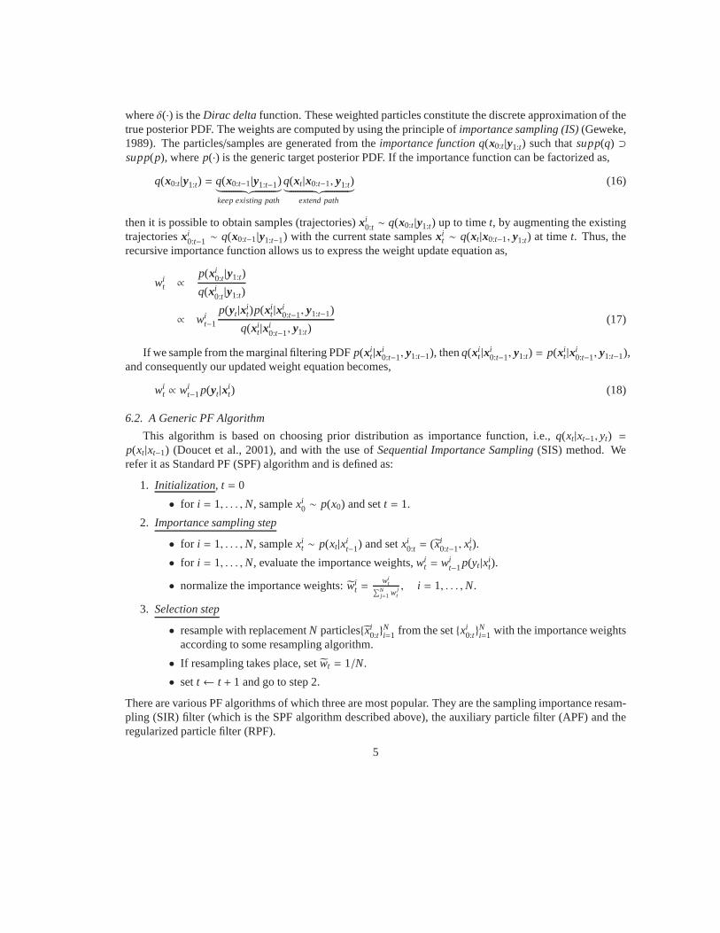
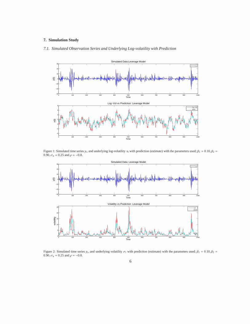
7.1. Simulated Observation Series and Underlying Log-volatility with Prediction

0 100 200 300 400 500 600 700 800 900 1000−30

−20

−10

0

10

20

30Simulated Data:Leverage Model

Time

y(t)

0 100 200 300 400 500 600 700 800 900 1000

−4

−2

0

2

4

6

8Log−Vol vs Prediction: Leverage Model

Time

x(t)

y

log−volpred

Figure 1: Simulated time seriesyt , and underlying log-volatilityxt with prediction (estimate) with the parameters used;β1 = 0.10, β2 =

0.90, σu = 0.25 andρ = −0.8.

0 100 200 300 400 500 600 700 800 900 1000−30

−20

−10

0

10

20

30Simulated Data: Leverage Model

Time

y(t)

0 100 200 300 400 500 600 700 800 900 10000

5

10

15

20

25

Volatility vs Prediction: Leverage Model

Time

vola

tility

y

volpred

Figure 2: Simulated time seriesyt , and underlying volatilityσt with prediction (estimate) with the parameters used;β1 = 0.10, β2 =

0.90, σu = 0.25 andρ = −0.8.

6

8. Applications on Real Data

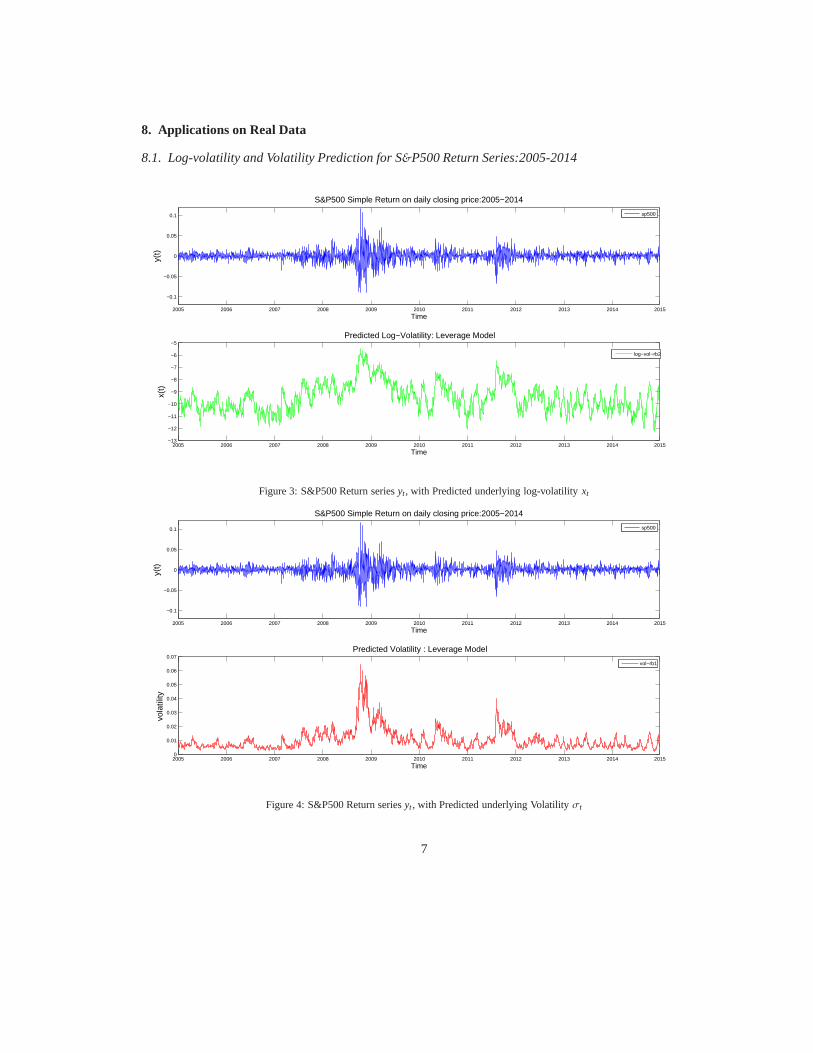
8.1. Log-volatility and Volatility Prediction for S&P500 Return Series:2005-2014

2005 2006 2007 2008 2009 2010 2011 2012 2013 2014 2015

−0.1

−0.05

0

0.05

0.1

S&P500 Simple Return on daily closing price:2005−2014

Time

y(t)

sp500

2005 2006 2007 2008 2009 2010 2011 2012 2013 2014 2015−13

−12

−11

−10

−9

−8

−7

−6

−5Predicted Log−Volatility: Leverage Model

Time

x(t)

log−vol−rb2

Figure 3: S&P500 Return seriesyt, with Predicted underlying log-volatilityxt

2005 2006 2007 2008 2009 2010 2011 2012 2013 2014 2015

−0.1

−0.05

0

0.05

0.1

S&P500 Simple Return on daily closing price:2005−2014

Time

y(t)

sp500

2005 2006 2007 2008 2009 2010 2011 2012 2013 2014 20150

0.01

0.02

0.03

0.04

0.05

0.06

0.07Predicted Volatility : Leverage Model

Time

vola

tility

vol−rb1

Figure 4: S&P500 Return seriesyt , with Predicted underlying Volatilityσt

7

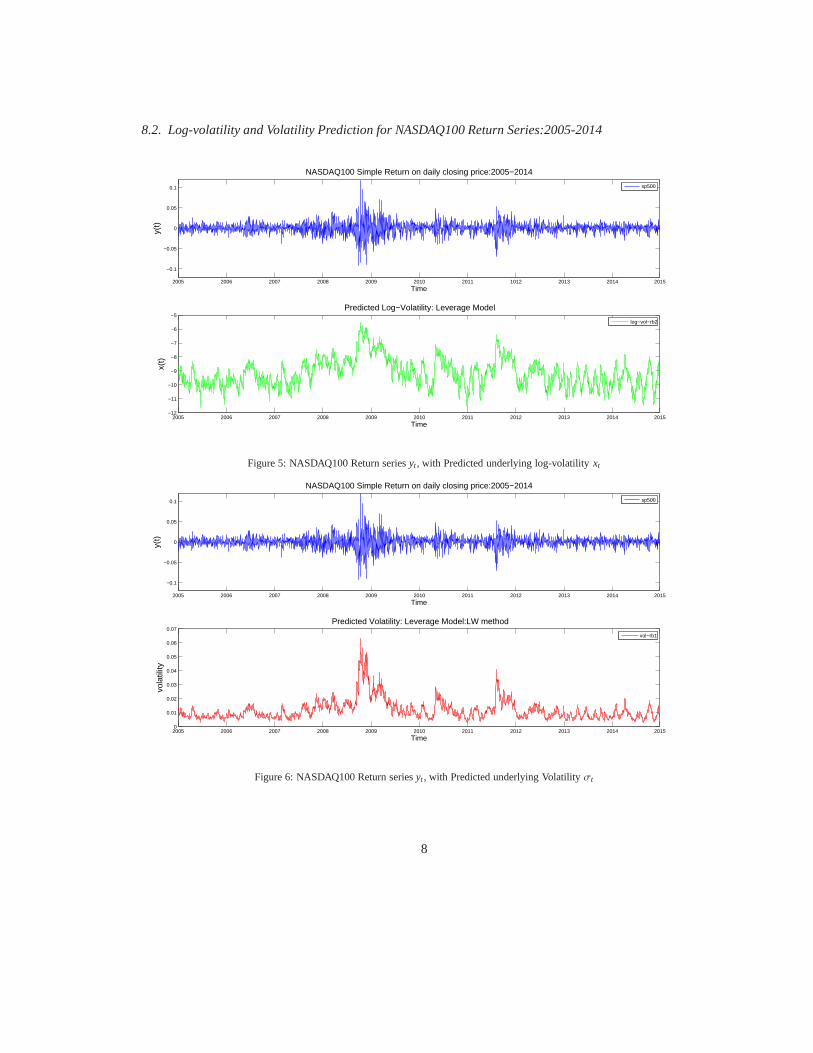
8.2. Log-volatility and Volatility Prediction for NASDAQ100 Return Series:2005-2014

2005 2006 2007 2008 2009 2010 2011 1012 2013 2014 2015

−0.1

−0.05

0

0.05

0.1

NASDAQ100 Simple Return on daily closing price:2005−2014

Time

y(t)

2005 2006 2007 2008 2009 2010 2011 2012 2013 2014 2015−12

−11

−10

−9

−8

−7

−6

−5Predicted Log−Volatility: Leverage Model

Time

x(t)

sp500

log−vol−rb2

Figure 5: NASDAQ100 Return seriesyt, with Predicted underlying log-volatilityxt

2005 2006 2007 2008 2009 2010 2011 2012 2013 2014 2015

−0.1

−0.05

0

0.05

0.1

NASDAQ100 Simple Return on daily closing price:2005−2014

Time

y(t)

2005 2006 2007 2008 2009 2010 2011 2012 2013 2014 20150

0.01

0.02

0.03

0.04

0.05

0.06

0.07Predicted Volatility: Leverage Model:LW method

Time

vola

tility

sp500

vol−rb1

Figure 6: NASDAQ100 Return seriesyt , with Predicted underlying Volatilityσt

8

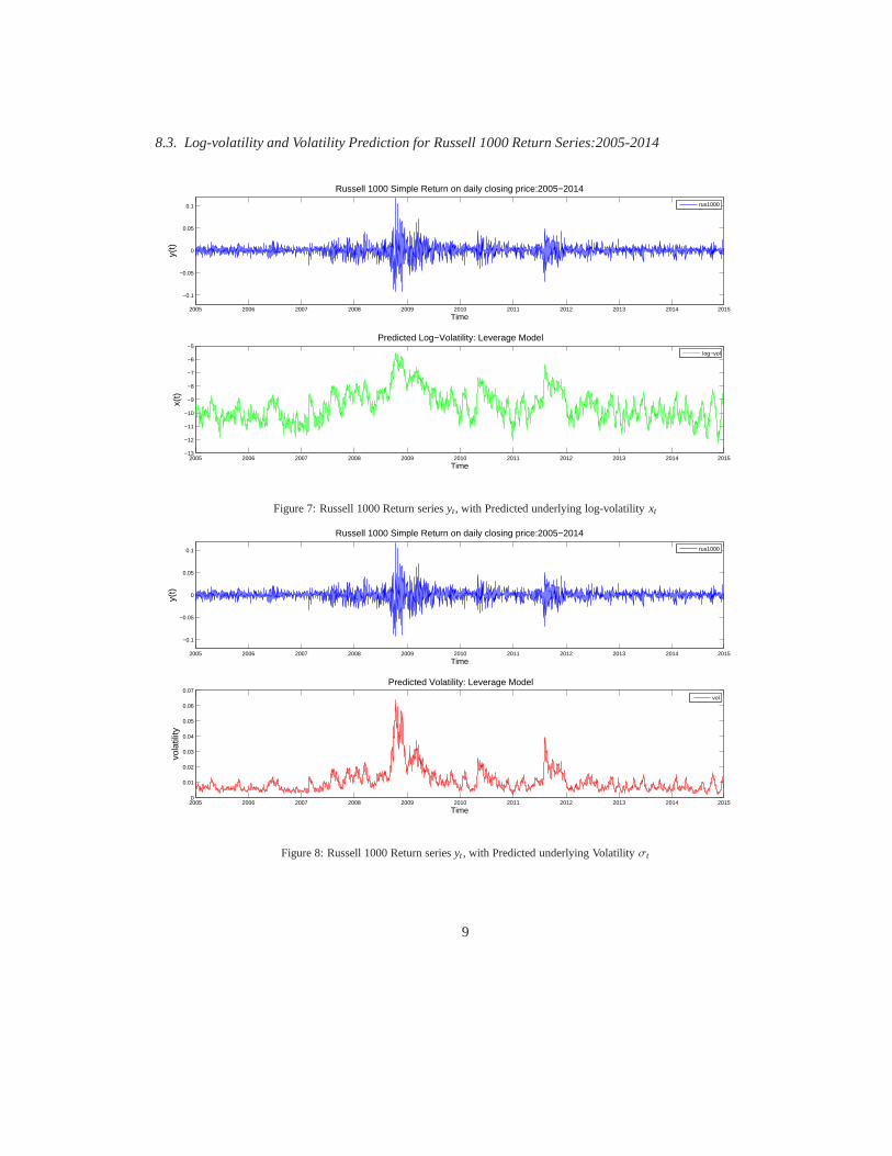
8.3. Log-volatility and Volatility Prediction for Russell1000 Return Series:2005-2014

2005 2006 2007 2008 2009 2010 2011 2012 2013 2014 2015

−0.1

−0.05

0

0.05

0.1

Russell 1000 Simple Return on daily closing price:2005−2014

Time

y(t)

2005 2006 2007 2008 2009 2010 2011 2012 2013 2014 2015−13

−12

−11

−10

−9

−8

−7

−6

−5Predicted Log−Volatility: Leverage Model

Time

x(t)

rus1000

log−vol

Figure 7: Russell 1000 Return seriesyt, with Predicted underlying log-volatilityxt

2005 2006 2007 2008 2009 2010 2011 2012 2013 2014 2015

−0.1

−0.05

0

0.05

0.1

Russell 1000 Simple Return on daily closing price:2005−2014

Time

y(t)

2005 2006 2007 2008 2009 2010 2011 2012 2013 2014 20150

0.01

0.02

0.03

0.04

0.05

0.06

0.07Predicted Volatility: Leverage Model

Time

vola

tility

rus1000

vol

Figure 8: Russell 1000 Return seriesyt , with Predicted underlying Volatilityσt

9

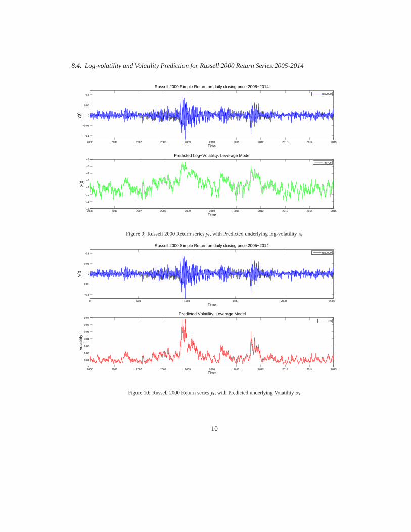
8.4. Log-volatility and Volatility Prediction for Russell2000 Return Series:2005-2014

2005 2006 2007 2008 2009 2010 2011 2012 2013 2014 2015

−0.1

−0.05

0

0.05

0.1

Russell 2000 Simple Return on daily closing price:2005−2014

Time

y(t)

2005 2006 2007 2008 2009 2010 2011 2012 2013 2014 2015−12

−11

−10

−9

−8

−7

−6

−5Predicted Log−Volatility: Leverage Model

Time

x(t)

rus2000

log−vol

Figure 9: Russell 2000 Return seriesyt, with Predicted underlying log-volatilityxt

0 500 1000 1500 2000 2500

−0.1

−0.05

0

0.05

0.1

Russell 2000 Simple Return on daily closing price:2005−2014

Time

y(t)

2005 2006 2007 2008 2009 2010 2011 2012 2013 2014 20150

0.01

0.02

0.03

0.04

0.05

0.06

0.07Predicted Volatility: Leverage Model

Time

vola

tility

rus2000

vol

Figure 10: Russell 2000 Return seriesyt, with Predicted underlying Volatilityσt

10

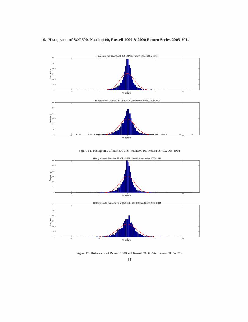
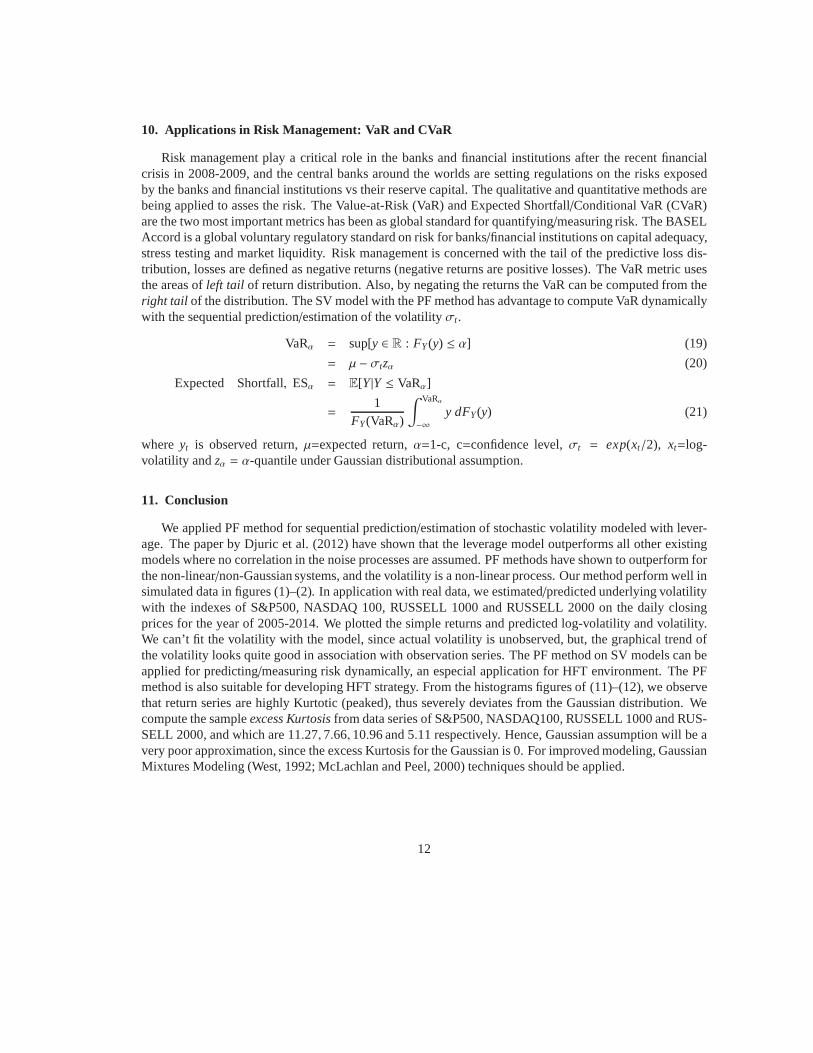
9. Histograms of S&P500, Nasdaq100, Russell 1000 & 2000 Return Series:2005-2014

−10 −5 0 5 100

50

100

150

200

250

300Histogram with Gaussian Fit of S&P500 Return Series:2005−2014

% return

freq

uenc

y

−10 −5 0 5 100

50

100

150

200

250

300Histogram with Gaussian Fit of NASDAQ100 Return Series:2005−2014

% return

freq

uenc

y

Figure 11: Histograms of S&P500 and NASDAQ100 Return series:2005-2014

−10 −5 0 5 100

50

100

150

200

250

300Histogram with Gaussian Fit of RUSSELL 1000 Return Series:2005−2014

% return

freq

uenc

y

−10 −5 0 5 100

50

100

150

200

250

300Histogram with Gaussian Fit of RUSSELL 2000 Return Series:2005−2014

% return

freq

uenc

y

Figure 12: Histograms of Russell 1000 and Russell 2000 Return series:2005-2014

11

10. Applications in Risk Management: VaR and CVaR

Risk management play a critical role in the banks and financial institutions after the recent financialcrisis in 2008-2009, and the central banks around the worldsare setting regulations on the risks exposedby the banks and financial institutions vs their reserve capital. The qualitative and quantitative methods arebeing applied to asses the risk. The Value-at-Risk (VaR) andExpected Shortfall/Conditional VaR (CVaR)are the two most important metrics has been as global standard for quantifying/measuring risk. The BASELAccord is a global voluntary regulatory standard on risk forbanks/financial institutions on capital adequacy,stress testing and market liquidity. Risk management is concerned with the tail of the predictive loss dis-tribution, losses are defined as negative returns (negativereturns are positive losses). The VaR metric usesthe areas ofleft tail of return distribution. Also, by negating the returns the VaR can be computed from theright tail of the distribution. The SV model with the PF method has advantage to compute VaR dynamicallywith the sequential prediction/estimation of the volatilityσt.

VaRα = sup[y ∈ R : FY(y) ≤ α] (19)

= µ − σtzα (20)

Expected Shortfall, ESα = E[Y|Y ≤ VaRα]

=1

FY(VaRα)

∫ VaRα

−∞

y dFY(y) (21)

where yt is observed return,µ=expected return,α=1-c, c=confidence level,σt = exp(xt/2), xt=log-volatility andzα = α-quantile under Gaussian distributional assumption.

11. Conclusion

We applied PF method for sequential prediction/estimation of stochastic volatility modeled with lever-age. The paper by Djuric et al. (2012) have shown that the leverage model outperforms all other existingmodels where no correlation in the noise processes are assumed. PF methods have shown to outperform forthe non-linear/non-Gaussian systems, and the volatility is a non-linear process. Our method perform well insimulated data in figures (1)–(2). In application with real data, we estimated/predicted underlying volatilitywith the indexes of S&P500, NASDAQ 100, RUSSELL 1000 and RUSSELL 2000 on the daily closingprices for the year of 2005-2014. We plotted the simple returns and predicted log-volatility and volatility.We can’t fit the volatility with the model, since actual volatility is unobserved, but, the graphical trend ofthe volatility looks quite good in association with observation series. The PF method on SV models can beapplied for predicting/measuring risk dynamically, an especial application for HFT environment. The PFmethod is also suitable for developing HFT strategy. From the histograms figures of (11)–(12), we observethat return series are highly Kurtotic (peaked), thus severely deviates from the Gaussian distribution. Wecompute the sampleexcess Kurtosisfrom data series of S&P500, NASDAQ100, RUSSELL 1000 and RUS-SELL 2000, and which are 11.27, 7.66, 10.96 and 5.11 respectively. Hence, Gaussian assumption will be avery poor approximation, since the excess Kurtosis for the Gaussian is 0. For improved modeling, GaussianMixtures Modeling (West, 1992; McLachlan and Peel, 2000) techniques should be applied.

12

References

Anderson, B., Moore, J., 1979. Optimal Filtering. Dover Publishing Inc.Arulampalam, M.S., Maskell, S., Gordon, N., Clapp, T., 2002. A tutorial on particle filters for online nonlinear/non-gaussian bayesian

tracking. IEEE Transactions on Signal Processing 50, 174–188.Black, F., 1976. Studies of stock market volatility changes. proceeding of the American Statistical Association. Bussiness and

Economic Statistics Section , 177–181.Black, F., Scholes, M., 1972. The valuation of option contracts and a test of market efficiency. The Journal of Finance 27, 399–418.Bollerslev, T., 1986. Generalized auto regressive conditional heteroscedasticity. Journal of Econometrics 31, 307–327.Box, G., Tiao, G., 1992. Bayesian Inference in Statistical Analysis. John Wiley and Sons, Inc.Casella, G., Robert, C.P., 1996. Rao-Blackwellization of sampling schemes. Biometrika 84, 81–94.Clark, P., 1973. A subordinated stochastic process model with finite variance for speculative prices. Econometrica 41,135–155.Crisan, D., Doucet, A., 2002. A survey of convergence results on particle filtering methods for practitioners. IEEE Transactions on

Signal Processing 50, 736–746.Djuric, P., Bugallo, M., 2009. ”Particle Filtering ” in Advances in Adaptive Filtering. Wiley & Sons. chapter 1.Djuric, P.M., Khan, M., Johnston, D.E., 2012. Particle filtering of stochastic volatility modeled with leverage. IEEE Journal of

Selected Topics in signal Processing 6, 327–336.Djuric, P.M., Kotecha, J.H., Zhang, J., Huang, Y., Ghirmai,T., Bugallo, M., Miguez, J., 2003. Particle filtering. IEEE Signal Processing

Magazine 20, 19–38.Doucet, A., de Freitas, N., Gordon, N. (Eds.), 2001. Sequential Monte Carlo Methods in Practice. Springer, New York.Doucet, A., Godsill, S., Andrieu, C., 2000. On sequential monte carlo sampling methods for bayesian filtering. Statistics and

Computing. 10, 197–208.Engle, R., 1982. Autoregressive conditional heteroscedasticity with estimates of the variance of the united kingdom inflation. Econo-

metrica 50, 987–1007.Geweke, J., 1989. Bayesian inference in econometrics models using monte carlo integration. Econometrica 57, 1317–1339.Ghysels, E., Harvey, A., Renault, E., 1996. ”Stochastic Volatility” in Handbook of Statistics, Statistical Method in Finance. Amster-

dam: North-Hollandl. chapter 14. pp. 119–191.Gordon, N., Salmond, D., Smith, A., 1993. Novel approach to nonlinear/non-Gaussian Bayesian state estimation. IEE proceedings-F

140, 107–113.Jacquier, E., Polson, N., Ross, P., 2004. Bayesian analysisof stochastic volatility models with fat-tails and correlated errors. Journal

of Econometrics 122, 185–212.Kalman, R.E., 1960. A new approach to linear filtering and prediction problems. Transactions of the ASME-Journal of Basic

Engineering 82, 35–45.Khan, M., 2011. Simulation-Based Sequential Bayesian Filtering with Rao-Blackwellization Applied to Nonlinear Dynamic State

Space Models. LAP LAMBERT Academic Publishing.Lehmann, E., 1991. Theory of Point Estimation. Wadsworth & Books.Liu, J., West, M., 2001. ”Combined Parameter and State Estimation in Simulation Based Filtering” in Sequential Monte Carlo Methods

in Practice. Springer. chapter 10.Maskell, S., 2004. ”An Introduction to Particle Filters” inState Space and Unobserved Component Models. Cambridge University

Press. chapter 3.McLachlan, G., Peel, D., 2000. Finite Mixture Models. 1st ed., Wiley & Sons.Nelson, D.B., 1991. Conditional heteroscedasticity in asset returns: A new approach. Econometrica 59, 347–370.Rosenberg, B., 1972. The behavior of random variable with nonstationary variance and the distribution of security prices. University

of California, Berkeley (Included in Stochastic Volatility: Selected Reading (ed Neil Shephard), Oxfor University Press, 2005) .Shephard, N., 1996. ”Ststistical aspects of ARCH and stochastic volatility” in Time Series Modles in Econometrics, Finance and other

fields. Chapman & Hall. chapter 1. pp. 1–67.Sorenson, H.W., Alspach, D.L., 1971. Recursive bayesian estimation using gaussian sums. Automatica 7, 465–479.Taylor, S., 1982. ”Financial returns modelled by the product of two stochastic processes-a study of daily sugar prices”in Time Series

Analysis: Theory and Parctice. Amsterdam:North-Holland.chapter 1. pp. 203–226.Taylor, S., 2005. Asset Price Dynamics, Volatility, and Prediction. Princeton University Press.West, M., 1992. Modelling with mixtures. Bayesian Statistics 4, 503–524.yu, J., 2005. On leverage in a stochastic volatility model. Journal of Econometrics 127, 165–178.

13