application of cellular automaton model to advanced ...space.ustc.edu.cn/users...spacing-oriented...

1. Introduction

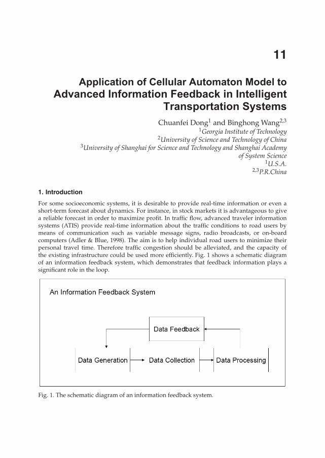
For some socioeconomic systems, it is desirable to provide real-time information or even ashort-term forecast about dynamics. For instance, in stock markets it is advantageous to givea reliable forecast in order to maximize profit. In traffic flow, advanced traveler informationsystems (ATIS) provide real-time information about the traffic conditions to road users bymeans of communication such as variable message signs, radio broadcasts, or on-boardcomputers (Adler & Blue, 1998). The aim is to help individual road users to minimize theirpersonal travel time. Therefore traffic congestion should be alleviated, and the capacity ofthe existing infrastructure could be used more efficiently. Fig. 1 shows a schematic diagramof an information feedback system, which demonstrates that feedback information plays asignificant role in the loop.

Fig. 1. The schematic diagram of an information feedback system.

Chuanfei Dong1 and Binghong Wang2,3

1Georgia Institute of Technology2University of Science and Technology of China

3University of Shanghai for Science and Technology and Shanghai Academyof System Science

1U.S.A.2,3P.R.China

Application of Cellular Automaton Model to Advanced Information Feedback in Intelligent

Transportation Systems

11

Physics, other sciences and technologies meet at the frontier area of interdisciplinary research(Helbing, 1996; Chowdhury et al., 2000; Helbing, 2001; Nagatani, 2002). The concepts andtechniques of physics are being applied to such complex systems as traffic systems. Alot of theories have been proposed such as car-following theory (Rothery, 1992), kinetictheory (Prigogine & Andrews, 1960; Paveri-Fontana, 1975; Helbing & Treiber, 1998) andparticle-hopping theory ( Nagel & Schreckenberg, 1992; Biham et al., 1992; Blue & Adler, 2001).These theories provide insights that help traffic engineers and other professionals to bettermanage congestion. Therefore these theories indirectly make contributions to alleviatingtraffic congestion and enhancing the capacity of existing infrastructure. Although dynamics oftraffic flow with real-time traffic information have been extensively investigated (Friesz et al.,1989; Arnott et al., 1991; Ben-Akiva et al., 1991; Mahmassani & Jayakrishnan, 1991; Kachroo& Özbay, 1996; Yokoya, 2004), finding out a more efficient feedback strategy is still an overalltask. Recently, some information feedbacks have been proposed to investigate the two-routescenario with the same length. Wahle et al. (2000 & 2002) firstly investigated the two-routescenario with travel time feedback strategy (TTFS). Subsequently, Lee et al. (2001) studied theeffect of a different type of information feedback (MVFS), i.e. instantaneous average velocity.Wang et al. (2005) proposed a third type of information feedback (CCFS), i.e. instantaneouscongestion coefficient which is defined as

C =q

∑i=1

n2i . (1)

where, ni stands for vehicle number of the ith congestion cluster in which cars are close to eachother without a gap between any two of them; q is the number of congestion clusters on theroute. Then Dong et al. (2010b) put forward another type of information feedback (WCCFS),i.e. instantaneous weighted congestion coefficient which is defined as

Cw =p

∑i=1

F(nm)n2i . (2)

where the definition of ni is the same as above, F(nm) is the weight function, andnm stands forthe position of the ith congestion cluster. Here, we use the result of median rounding �nm� ofthe ith congestion cluster to represent its position. Furthermore, in order to provide road userswith better guidance, Dong et al. (2009a; 2009b; 2010a; 2010d) proposed another two typesof information feedback strategies named corresponding angle feedback strategy (CAFS)and prediction feedback strategy (PFS), respectively. The corresponding angle coefficient isdefined as

Cθ =q

∑i=1

θ2i =

q

∑i=1

(arctan(

n f irstiH

)− arctan(n f irst

i − li

H)

)2

. (3)

where n f irsti stands for the position of the first vehicle in the ith congestion cluster, in which

vehicles are close to each other without a gap between any two of them. li and θi denotethe length and the weight (corresponding angle) of the ith congestion cluster, respectively.H denotes the vertical distance from point T to the route (see Fig.2). In this chapter, we setH = 100. PFS is based on CCFS, and the predicted congestion coefficient (Cp) is defined as:

Cp(t) = C(t + Δt) =q

∑i=1

n2i (t + Δt). (4)

238 Cellular Automata - Simplicity Behind Complexity

Fig. 2. Angles corresponding to different congestion clusters on the lane.

which indicates that PFS uses future road condition (the value of congestion coefficient C attime t + Δt) as feedback information.It has been proved that TTFS is the worst one which brings a lag effect to make it impossibleto provide the road users with the real situation of each route (Lee et al., 2001); CCFS is moreefficient than MVFS because the random brake mechanism of the Nagel-Schreckenberg (NS)model (Nagel & Schreckenberg, 1992) brings fragile stability of velocity (Wang et al., 2005);WCCFS is more efficient than CCFS for the reason that CCFS does not take the weights ofdifferent parts of the route into consideration (Dong et al., 2010b). However, WCCFS is still notthe best one due to the fact that the weight function F(nm) does not contain any informationrelated to the length of the congestion cluster while the corresponding angle θ takes boththe length and route location of each cluster into account (Dong & Ma, 2010a). Though theroad capacity adopting PFS is the best one among these feedback strategies (Dong et al.,2009a; Dong et al., 2009b; Dong et al., 2010d), the validity of PFS depends on the length ofthe route when the traffic system is multi-route (Dong et al., 2010d). Also, PFS is not easy torealize since it needs predicted road data, which will be discussed in detail in the followingparagraphs. We report the simulation results adopting six different feedback strategies TTFS,MVFS, CCFS, WCCFS, CAFS and PFS in a two-route scenario with a single route followingthe NS mechanism.The chapter is arranged as follows: In Section 2, several cellular automaton models of trafficflow will be mentioned including some analytical studies and a two-route scenario is brieflyintroduced, together with six feedback strategies of TTFS, MVFS, CCFS, WCCFS, CAFS andPFS all depicted in detail. In Section 3, some simulation results will be presented and discussedbased on the comparison of six different feedback strategies. In Section 4, we will make someconclusions.

2. The model and feedback strategies

A. NS mechanismRecently, a lot of cellular automaton models are proposed such as NS model (Nagel &Schreckenberg, 1992), FI model (Fukui & Ishibashi, 1996), VDR model (Barlovic et al., 1998),VE model (Li et al., 2001), BL model (Knospe et al., 2000), VE model (Li et al., 2001),Kerner-Klenov-Wolf model (Kerner et al., 2002; Kerner & Klenov, 2004; Kerner, 2004), FMCDmodel (Jiang & Wu, 2003; Jiang & Wu, 2005), VDDR model (Hu et al., 2007), and VA model(Gao et al., 2007). Also, a lot of analytical works based on statistical physics, such as the

239Application of Cellular Automaton Model toAdvanced Information Feedback in Intelligent Transportation Systems

spacing-oriented mean field theory, have been studied to investigate fundamental diagramsand asymptotic behavior of CA models, i.e., NS model, FI model, and NS & FI combined CAmodel (Wang et al., 2000a; Wang et al., 2000b; Mao et al., 2003; Wang et al., 2003; Wang etal., 2001; Fu et al., 2007). Among these CA models, the NS model is so far the most popularand simplest cellular automaton model in analyzing the traffic flow (Nagel & Schreckenberg,1992; Chowdhury et al., 2000; Helbing, 2001; Nagatani, 2002; Wang et al., 2002), where theone-dimension CA with periodic boundary conditions is used to investigate highway andurban traffic. This model can reproduce the basic features of real traffic like stop-and-gowave, phantom jams, and the phase transition on a fundamental diagram that plots vehicleflow versus density. Thus we still adopt NS model when comparing the effects of differentfeedback strategies in this chapter. In the following paragraphs, the NS mechanism will bebriefly introduced as a basis of analysis.The road is subdivided into cells (sites) with a length of Δx=7.5 m. The route length is set tobe L = 2000 cells (corresponding to 15 km). N denotes the total number of vehicles on a singleroute of length L. The vehicle density can be defined as ρ=N/L. A time step corresponds toΔt = 1s, the typical time a driver needs to react. gn(t) refers to the number of empty sitesin front of the nth vehicle at time t, and vn(t) denotes the speed of the nth vehicle, i.e., thenumber of sites that the nth vehicle moves during the time step t. In the present paper, weset the maximum velocity vmax = 3 cells/time step (corresponding to 81 km/h and thus areasonable value) for simplicity. The rules for updating the position x of a car are as follows. (i)Acceleration: vi = min(vi + 1, vmax). (ii) Deceleration: v

′i = min(vi, gi) so as to avoid collisions,

where gi is the spacing in front of the ith vehicle. (iii) Random brake: with a certain probabilityp that v

′′i = max(v

′i − 1, 0). (iv) Movement: xi = xi + v

′′i .

The fundamental diagram characterizes the basic properties of the NS model which has tworegimes called "free-flow" phase and "jammed" phase. The critical density, basically dependingon the random brake probability p, divides the fundamental diagram to these two phases.The transition such as from "free-flow" phase to "jammed" phase is called transition on afundamental diagram (Nagel & Schreckenberg, 1992).B. Two-route scenarioRecently, Wahle et al. (2000) investigated a two-route model. In their model, a percentage ofdrivers (referred to as dynamic drivers) choose one of the two routes according to the real-timeinformation displayed on the roadside. In their model, the two routes A and B are of the samelength L. A new vehicle will be generated at the entrance of the traffic system at each timestep. If a driver is a so-called static one, he enters a route at random ignoring any advice.The density of dynamic and static travelers are Sdyn and 1 − Sdyn, respectively. Once a vehicleenters one of two routes, the motion of it will follow the dynamics of the NS model. In oursimulation, a vehicle will be removed after it reaches the end point. It is important to notethat if a vehicle cannot enter the preferred route, it will wait till the next time step rather thanentering the un-preferred route.The simulations are performed by the following steps: first, we set the routes and boardsempty; second, let vehicles enter the routes randomly during the initial 100 time steps; third,after the vehicles enter the routes, according to four different feedback strategies, informationwill be generated, transmitted, and displayed on the board at each time step. Finally, thedynamic road users will choose the route with better conditions according to the dynamicinformation at the entrance of two routes.C. Related definitions


The road conditions can be characterized by the fluxes of two routes. The flux of the ith routeis defined as follows:

Fi = Vimeanρi = Vi

meanNiLi

(5)

where Li represents the length of the ith route, Vimean and Ni denote the mean velocity of all

the vehicles and the vehicle number on the ith route, respectively. In this chapter, the physicalsense of flux F is the number of vehicles passing the exit of the traffic system each time step.Therefore the larger the value of F, the better processing capacity the traffic system has.We assume the two-route system has only one entrance and one exit as shown in Fig.3. Inreality, there are different paths for drivers to choose from one place to another place. In thischapter, we focus on a two-route system. Different drivers departing from the same placecould choose two different paths to get to the same destination which corresponds to the “oneentrance and one exit” system. Thus the road condition in present work is closer to realitythan some previous works (Wahle et al.,2000; Lee et al., 2001; Wang et al., 2005). The rules atthe exit of the two-route system are as follows:

Fig. 3. The one entrance and one exit two-route traffic system.

a) The special velocity update mechanism for the vehicle nearest to the exit:

i velocity(t)=Min(velocity(t)+1,3), (probability: 75%);ii velocity(t)=Max(velocity(t)-1,0), (probability: 25%);

b) Rules at the exit when vehicles competing for driving out:

i At the end of two routes, the vehicle nearer to the exit goes first.ii If the vehicles at the end of two routes have the same distance to the exit, the faster a

vehicle drives, the sooner it goes out.iii If the vehicles at the end of two routes have the same speed and distance to the exit, the

vehicle in the route which has more vehicles drives out first.iv If the rules (i), (ii) and (iii) are satisfied at the same time, then the vehicles go out

randomly.

c) velocity(t)=position(t)-position(t-1), where position(t)=L=2000; (valid only for the vehiclesfailed in competing for driving out at exit);

Here we want to stress that the vehicle nearest to the exit will not obey the NS mechanism butthe special mechanism as shown in rule (a). However, vehicles following the vehicle closestto the exit still obey the NS mechanism. One should also be aware that if the vehicle nearest


to the exit does not compete with the vehicle on the other route for driving out or wins in thecompetition, the vehicle will ignore rule (c). The special velocity update mechanism (rule (a))is equivalent to the situation that 75% drivers exhibit aggressive behavior and 25% driversexhibit timid behavior near the exit, which is similar to the recent work studied by Laval &Leclercq (2010). Please note that drivers exhibit timid behavior may also exhibit aggressivebehavior at next time step otherwise the timid drivers may stop at the exit all the time. Thenwe describe six different feedback strategies as follows:TTFS: The information of travel time on the board is set to be zero until one car leave the trafficsystem. Each vehicle will be recorded the time when it enters and leaves one of the routes. Weuse the difference between this two values as the feedback information. A new dynamic driverwill choose the road with shorter time shown on the information board.MVFS: Every time step, the traffic control center will receive the velocity of each vehicle on theroute from GPS. They will deal with the information and display the mean velocity of vehicleson each route on the information board. Road users at the entrance will choose one road withlarger mean velocity.CCFS: Every time step, the traffic control center will receive the position of each vehicle on theroute from GPS. The work of the traffic control center is to compute the congestion coefficientof each route and display it on the information board. Road users at the entrance will chooseone road with smaller congestion coefficient. The congestion coefficient is defined as

C =q

∑i=1

nwi . (6)

where ni stands for vehicle number of the ith congestion cluster in which cars are close to eachother without a gap between any two of them, and q denotes the total number of congestionclusters on one route. Every cluster is evaluated by a weight w, where w = 2 and one cancheck out that w > 2 leads to the similar results with w = 2 (Wang et al., 2005).WCCFS: Every time step, the traffic control center will receive data from the navigation system(GPS) like CCFS, and the work of the center is to compute the congestion coefficient of eachroad with a reasonable weighted function and display it on the information board. Roadusers at the entrance will choose one road with smaller weighted congestion coefficient. Theweighted congestion coefficient is defined as Eq.(2).After we try some functions such as F(x) = cos(ax) + b and Gaussian function, we findF(x) = kx + b is the optimal one in terms of improving the capacity of the road. Here, weset b �= 0 for the reason that it will cause the absolute weight value of the first route sitealways to be the smallest when b = 0. In this chapter, we set b = 2.0. Then we get the functionas follows:

F(x) = k × x + b = k × nm

2000+ 2.0. (7)

Finally the expression of Cw becomes

Cw =q

∑i=1

F(nm)n2i =

q

∑i=1

(k × nm

2000+ 2.0)× n2

i . (8)

We also find that how efficient the new strategy to improve the road capacity depends on thevalue of the weight factor (slope - k) which we will discuss in detail in Section 3.CAFS: Every time step, the traffic control center will receive data from the navigation system(GPS) like CCFS. The work of the traffic control center is to compute the corresponding angle


of each congestion cluster (see Fig.2) on the lane, sum square of each corresponding angleup and display it on the information board. Road users at the entrance will choose one roadwith smaller corresponding angle coefficient. The corresponding angle coefficient is definedas Eq.(3).PFS: Every time step, the traffic control center will receive data from the navigation system(GPS) like CCFS. The work of the center is to compute the congestion coefficient of each route,simulate the future road condition based on the current road condition by using CCFS, anddisplay the results on the information board. Road users at the entrance will choose one routewith smaller predicted congestion coefficient. For example, if the prediction time, Tp, is 50seconds and the current time is the 100th second, the traffic control center will simulate theroad conditions in the next 50 seconds adopting CCFS, predict the road condition at the 150thsecond, and show the result on the information board at the entrance of the route. Finally, roadusers at the 100th second will choose one route with smaller predicted congestion coefficient atthe 150th second. By the same token, road users at the entrance at the 101th second will chooseone route with smaller predicted congestion coefficient at the 151th second like explainedabove. The predicted congestion coefficient is defined as Eq.(4).In the following section, performance by using six different feedback strategies will be shownand discussed in detail.

3. Simulation results

Fig.4 (a) shows the dependence of average flux on weight factor (k) by using WCCFS. As tothe routes’ processing capacity, we can see that in Fig.4 (a) there is a positive peak structure atthe vicinity of k ∼ -1.98. Thus we will use k=-1.98 in the following paragraphs. Then Eq.(8) willbecome Cw = ∑

qi=1(−1.98× nm

2000 + 2.0)× n2i . In Fig.4 (b), we present the weight value of each

site on one route. One can find the weight value of the entrance is much larger than that of theexit when using WCCFS and the reasons can be described as follows. First, in practice bothacceleration and deceleration shock waves travel at final velocities and – at least on average– vehicles tend to be more affected by local traffic conditions than by conditions far ahead onthe roadway. This suggests that greater weight should be given to traffic conditions on theupstream sections of each route. Second, the smaller weight value at the end of the route willalleviate the negative effect of congestion caused by the traffic jam.Since Fig.4 (a) shows the weight value of the entrance is larger than that of the exit whenadopting WCCFS, the point T located above the entrance of the route when adopting CAFS(see Fig.2) is reasonable. It makes the weight of the entrance the largest. Furthermore, thecorresponding angle of each congestion cluster can reflect not only the weight of the routebut also the length of the congestion cluster. Therefore the weight value is more reasonablethan before (Dong et al., 2010a). Fig.4 (c) shows the dependence of average flux on positionof the pillar (point T) by using CAFS. As to the routes’ processing capacity, we can see thatthe position of the pillar will directly affect the average flux. The average flux is much largerwhen point T locates at the entrance of the route while the value is pretty lower when pointT locates at the end of the lane. Thus the result shown by Fig.4(c) is in accordance with thatindicated by Fig.4 (a). Also, this can be understood as shown in Fig.5, where the congestioncluster on route A locates at the entrance of lane and the congestion cluster on route B locatesat the end of the lane. From Fig.5, we can see clearly that Cθ of route A is larger than that ofroute B, so the road user should enter route B instead of route A. If point T locate at the end ofthe route, Cθ of route A will smaller than that of route B, which will cause the vehicle to enterroute A. It will make the cluster larger or the vehicle even cannot enter the route.


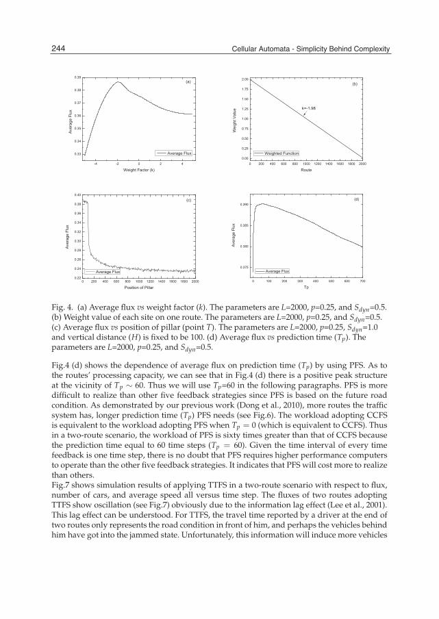
Fig. 4. (a) Average flux vs weight factor (k). The parameters are L=2000, p=0.25, and Sdyn=0.5.(b) Weight value of each site on one route. The parameters are L=2000, p=0.25, and Sdyn=0.5.(c) Average flux vs position of pillar (point T). The parameters are L=2000, p=0.25, Sdyn=1.0and vertical distance (H) is fixed to be 100. (d) Average flux vs prediction time (Tp). Theparameters are L=2000, p=0.25, and Sdyn=0.5.

Fig.4 (d) shows the dependence of average flux on prediction time (Tp) by using PFS. As tothe routes’ processing capacity, we can see that in Fig.4 (d) there is a positive peak structureat the vicinity of Tp ∼ 60. Thus we will use Tp=60 in the following paragraphs. PFS is moredifficult to realize than other five feedback strategies since PFS is based on the future roadcondition. As demonstrated by our previous work (Dong et al., 2010), more routes the trafficsystem has, longer prediction time (Tp) PFS needs (see Fig.6). The workload adopting CCFSis equivalent to the workload adopting PFS when Tp = 0 (which is equivalent to CCFS). Thusin a two-route scenario, the workload of PFS is sixty times greater than that of CCFS becausethe prediction time equal to 60 time steps (Tp = 60). Given the time interval of every timefeedback is one time step, there is no doubt that PFS requires higher performance computersto operate than the other five feedback strategies. It indicates that PFS will cost more to realizethan others.Fig.7 shows simulation results of applying TTFS in a two-route scenario with respect to flux,number of cars, and average speed all versus time step. The fluxes of two routes adoptingTTFS show oscillation (see Fig.7) obviously due to the information lag effect (Lee et al., 2001).This lag effect can be understood. For TTFS, the travel time reported by a driver at the end oftwo routes only represents the road condition in front of him, and perhaps the vehicles behindhim have got into the jammed state. Unfortunately, this information will induce more vehicles


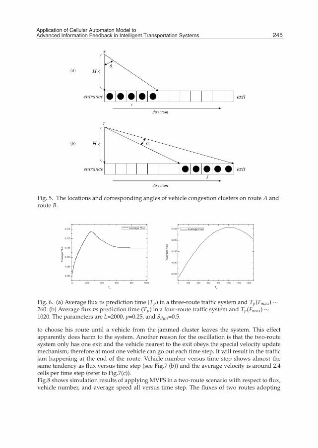
Fig. 5. The locations and corresponding angles of vehicle congestion clusters on route A androute B.

Fig. 6. (a) Average flux vs prediction time (Tp) in a three-route traffic system and Tp(Fmax) ∼260. (b) Average flux vs prediction time (Tp) in a four-route traffic system and Tp(Fmax) ∼1020. The parameters are L=2000, p=0.25, and Sdyn=0.5.

to choose his route until a vehicle from the jammed cluster leaves the system. This effectapparently does harm to the system. Another reason for the oscillation is that the two-routesystem only has one exit and the vehicle nearest to the exit obeys the special velocity updatemechanism; therefore at most one vehicle can go out each time step. It will result in the trafficjam happening at the end of the route. Vehicle number versus time step shows almost thesame tendency as flux versus time step (see Fig.7 (b)) and the average velocity is around 2.4cells per time step (refer to Fig.7(c)).Fig.8 shows simulation results of applying MVFS in a two-route scenario with respect to flux,vehicle number, and average speed all versus time step. The fluxes of two routes adopting


Fig. 7. (Color online)(a) Flux of each route with travel time feedback strategy. (b) Vehiclenumber of each route with travel time feedback strategy. (c) Average speed of each routewith travel time feedback strategy. The parameters are L=2000, p=0.25 and Sdyn=0.5.


MVFS showing oscillation (see Fig.8) is primarily due to two reasons. First, for MVFS, we havementioned that the NS model has a random brake scenario which causes the fragile stabilityof velocity, thus MVFS cannot completely reflect the real condition of routes. The other reasonfor the disadvantage of MVFS is that flux consists of two parts, mean velocity and vehicledensity, but MVFS only grasps one part and lacks the other part of flux (Wang et al., 2005).Also, the one exit structure of the traffic system and the special velocity update mechanismfor the vehicle closest to the exit can also cause oscillation as explained in the last paragraph.Vehicle number versus time step shows almost the same tendency as flux versus time step(see Fig.8 (b)) and the average velocity is around 2.3 cells per time step (refer to Fig.8(c)).Fig.9 show the dependence of flux, number of cars, average speed on time step by using CCFS.Compared with TTFS and MVFS, the performance of CCFS is good. The reason is primarilydue to that CCFS takes the congestion cluster effects into account by adding a weight to eachcluster. This can be explained by the fact that travel time of the last vehicle of the cluster fromthe entrance to the destination is obviously affected by the size of cluster. With the increasingof cluster size, travel time of the last vehicle will be longer, and the correlation between clustersize and travel time of the last vehicle is nonlinear. For simplicity, an exponent w is added tothe size of each cluster to be consistent with the nonlinear relationship. To some extent, CCFSreduces the oscillation, and increases the vehicle number of each route (see Fig.9 (a) & (b))while decreases the average velocity that is approximate to 2.2 cells per time step (refer toFig.9(c)).The dependence of flux, number of vehicles, average speed on time step by adopting WCCFSis shown in Fig.10. WCCFS further reduces the oscillation and increases the flux due to the factthat WCCFS takes the weights of different parts of the route into consideration. From Fig.4 (b)we can see that weight values at the end of the route are always smaller, which is equivalentto alleviating the negative effect of congestion caused by the traffic jam; therefore WCCFSmay improve the road condition. Compared to CCFS, the performance adopting WCCFS isimproved at some points, not only on the value but also the stability of the flux.Fig.11 shows the relationship between flux, number of vehicles, average speed and time stepby using CAFS. In contrast with CAFS, the fluxes of two routes adopting TTFS, MVFS, CCFSand WCCFS show larger oscillation (see Fig.7-10). This oscillation effect can be understoodfor several reasons besides those discussed above. First, TTFS, CCFS and MVFS cannotreflect the weights of different parts of the route. Additionally, though WCCFS can reflectthe route weights, the weighted function (F(nm)) is independent of the cluster length. Weuse the median rounding �nm� of the ith congestion cluster to represent its position whenadopting WCCFS. However, CAFS takes both the length and location of the congestion clusterinto account, which can give the road user with better guidance. For example, if there exitcongestion clusters at the end of both routes, the road user will choose the route with shortercluster length. The reason is that there is a positive correlation between the value of Cθ andthe length of the cluster when the locations of clusters are the same. If the clusters have thesame length but locate at different positions of the routes as shown in Fig.5, the road userwill choose route B with smaller Cθ. Compared to WCCFS, the performance adopting CAFSis further improved, not only on the value but also the stability of the flux.In Fig.11 (b), vehicle number versus time step shows that the routes’ accommodating capacityis greatly enhanced with an increase in average vehicle number. Thus perhaps the high fluxesof two routes with CAFS are mainly due to the increase of vehicle number. In Fig.11 (c),speed versus time step shows that although the speed is more stable by using CAFS, itbecomes lower than the other four strategies discussed above. The reason is that the routes’


Fig. 8. (Color online)(a) Flux of each route with mean velocity feedback strategy. (b) Vehiclenumber of each route with mean velocity feedback strategy. (c) Average speed of each routewith mean velocity feedback strategy. The parameters are L=2000, p=0.25 and Sdyn=0.5.


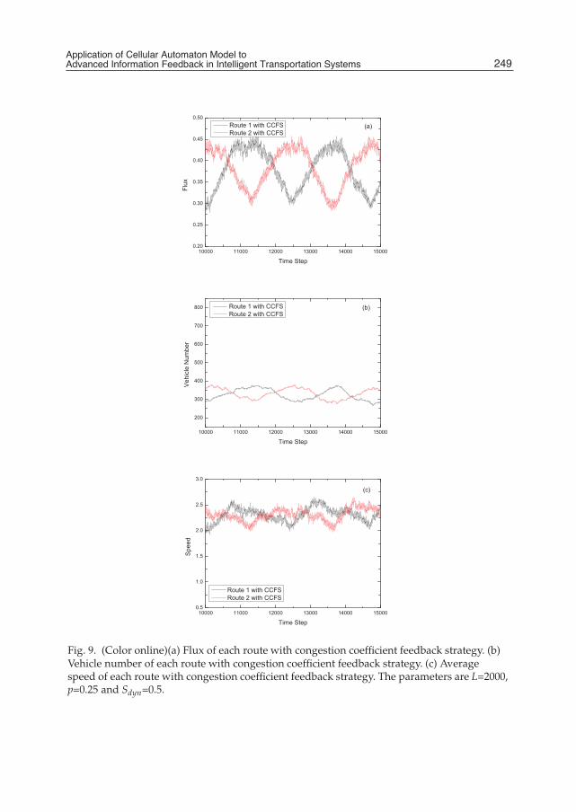
Fig. 9. (Color online)(a) Flux of each route with congestion coefficient feedback strategy. (b)Vehicle number of each route with congestion coefficient feedback strategy. (c) Averagespeed of each route with congestion coefficient feedback strategy. The parameters are L=2000,p=0.25 and Sdyn=0.5.


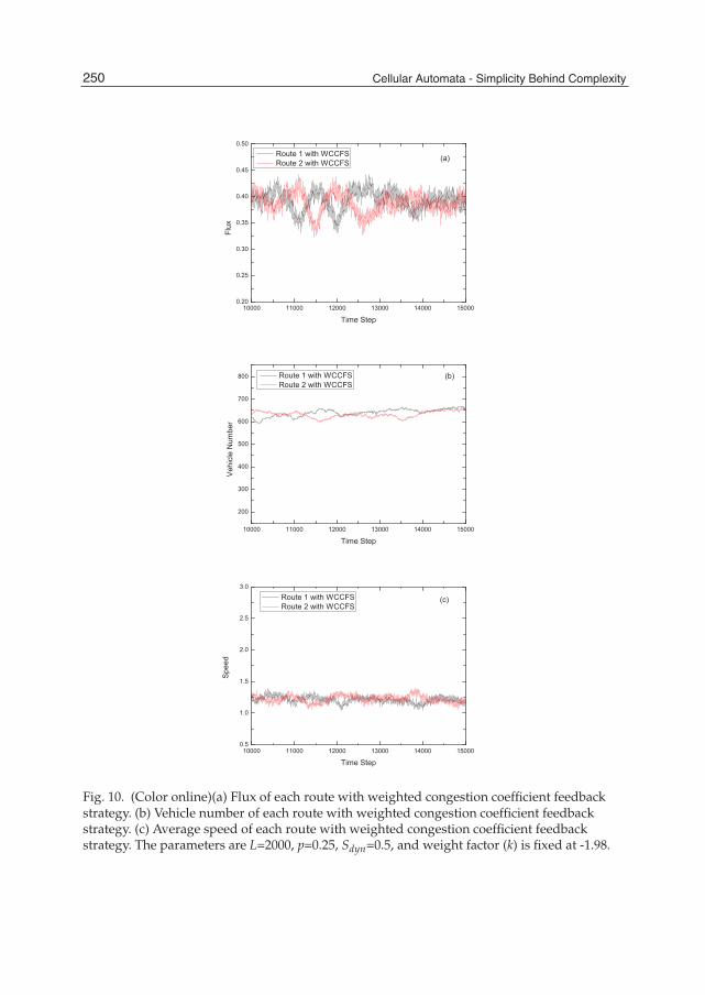
Fig. 10. (Color online)(a) Flux of each route with weighted congestion coefficient feedbackstrategy. (b) Vehicle number of each route with weighted congestion coefficient feedbackstrategy. (c) Average speed of each route with weighted congestion coefficient feedbackstrategy. The parameters are L=2000, p=0.25, Sdyn=0.5, and weight factor (k) is fixed at -1.98.


accommodating capacity by using CAFS is better than that of other four strategies, and atmost one vehicle can drive out each time step as explained before; therefore more cars thelane has, lower speeds the vehicles have. Fortunately, flux consists of two parts, mean velocityand vehicle density. Hence, as long as the vehicle number (because vehicle density is definedas ρ=N/L, and L is fixed at 2000, so ρ ∝ vehicle number (N)) is large enough, the flux can alsobe the largest.Fig.12 shows the dependence of flux, vehicle number, average speed on time step whenadopting PFS. The advantage of PFS is that it can predict the negative effects on the routecondition caused by traffic jams happened at the end of the route, try to avoid jammed stateto the best of its ability, and alleviate the negative effects as much as possible. Here, we wantto stress that though PFS try to avoid the jammed state, the structure of the traffic system (oneexit) and the special velocity update mechanism for the vehicle nearest to the exit still makejams happened at the end of the route occasionally. Also, this can explain the slight oscillationin Fig.12 (a).From Fig.12 (b) we know that the average vehicle number is around 760 by using PFS. Asto the routes’ stability, we know PFS is the optimal one, which means the vehicles shouldbe almost uniformly distributed on each route instead of being together at the end of theroutes. Furthermore, even there are 760 vehicles on each route, vehicles can still averagelyoccupy 2 ∼ 3 sites on each route because the total length of each route is fixed at 2000 sites.This indicates there are only 1 ∼ 2 sites between vehicles. Though the vehicles are almostdistributed separately on each lane, the one exit structure and the special velocity updatemechanism for the vehicle closest to the exit make jams still have a chance to happen at theend of the route. However, PFS can prevent jams from further expanding and alleviate thenegative effects as much as possible, so that the jammed state will disappear soon. So as toanalogize, even the jams happen again, the poor road condition will be relieved in a shorttime period.As to the low speed shown in Fig.12 (c), the reason is that the speed partially depends on thenumber of empty sites between two vehicles on the lane. The vehicle behind another vehiclecan move at most the current empty sites between them which is required by NS mechanism(Nagel & Schreckenberg, 1992). The routes’ accommodating capacity is the best by using PFS,indicating the speed adopting PFS the lowest. From the stability of the velocity, we infer thatthe vehicles should drive at almost uniform speeds on each route. Without consider otherfactors, the speed should be a little more than one (∼ 1.5) because there are only 1 ∼ 2 cellsbetween vehicles as mentioned above. If we take the random brake effects and the occasionaljams at the end of the route into account, the vehicles’ average velocity decreasing a littleis possible and reasonable. Thus, the average velocity Vavg ∼ 1 in this chapter could beunderstood. These analysis can also be applied to explain the low average velocity by usingWCCFS and CAFS.Someone may have doubts whether CAFS and PFS are really better than the other fourfeedback strategies due to the lower speed shown in Fig.11 (c) & Fig.12 (c). In order to makingthe readers understand more easily, we assume that the road network under study includesnot only the downstream corridor section displayed in Fig.3, but also a section upstream ofthe entrance where vehicles wait to enter the corridor (Dong et al., 2010c). Thus, we shouldtake into account the total travel time (ttot) that is the sum of driving time (tdriving) and waitingtime (twaiting) to evaluate the merits of these feedback strategies.

ttot = tdriving + twaiting (9)


Fig. 11. (Color online)(a) Flux of each route with corresponding angle feedback strategy. (b)Vehicle number of each route with corresponding angle feedback strategy. (c) Average speedof each route with corresponding angle feedback strategy. The parameters are L=2000,p=0.25, Sdyn=0.5, and vertical distance (H) is fixed at 100.


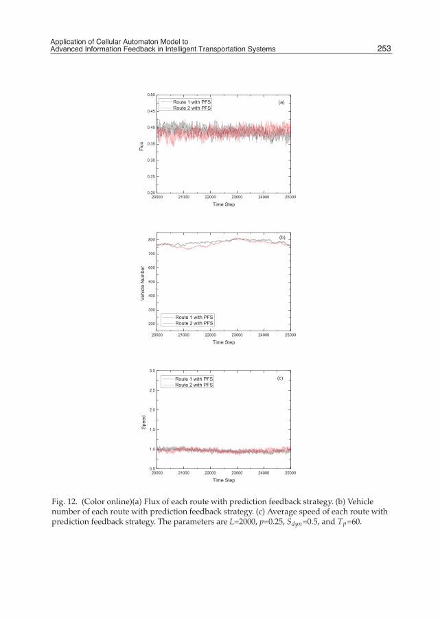
Fig. 12. (Color online)(a) Flux of each route with prediction feedback strategy. (b) Vehiclenumber of each route with prediction feedback strategy. (c) Average speed of each route withprediction feedback strategy. The parameters are L=2000, p=0.25, Sdyn=0.5, and Tp=60.


Total travel time (ttot): ttot is the time period that vehicles spend on the whole traffic systemthat includes the upstream and downstream corridor sections. Flux is a very good proxy toevaluate the total travel time, because it can be understood as the number of vehicles passingthe exit each time step. The more vehicles pass the exit during a fixed time period, the shortertime these vehicles spend on the traffic system. For example, there are totally N vehicles in thesection upstream of the entrance, then the average flux of the traffic system is

Favg = N/ttot (Nth vehicle) ≈ n/ttot (nth vehicle), n ∈ [1, N]. (10)

Here, one should be aware that the average flux value is stable, thus the approximation inEq.(10) is valid. Therefore the travel time adopting CAFS and PFS is shorter than the other fourfeedback strategies for the fact that the flux adopting CAFS and PFS are larger (see Fig.13).Driving time (tdriving): tdriving is the time period vehicles spend on the downstream routesection displayed in Fig.3. It is obvious that driving time of CAFS and PFS is longer thanthe other four feedback strategies since the speeds v adopting CAFS and PFS are lower asshown in Fig.11 (c) & Fig.12 (c) (the length of the route L is fixed at 2000, thus tdriving = L/v).Waiting time (twaiting): twaiting is the time period vehicles waiting in the upstream route section.Since the total travel time (ttot) is the sum of waiting time (twaiting) and driving time (tdriving)as shown in Eq.(9), the waiting time adopting CAFS and PFS is shorter on the basis of aboveanalysis.Fig.13 shows that the average flux fluctuates feebly with a persisting increase of dynamictravelers by using six different strategies. As to the routes’ processing capacity, PFS is provedto be the best one because the flux is always the largest at each Sdyn value and even increaseswith a persisting increase of dynamic travelers.

4. Conclusion

We obtain the simulation results of applying six different feedback strategies, i.e., TTFS, MVFS,CCFS, WCCFS, CAFS and PFS in a two-route scenario all with respect to flux, number ofvehicles, speed, and average flux versus Sdyn. We also show the results about average fluxversus weight factor (k) by adopting WCCFS, average flux versus position of pillar (pointT) by adopting CAFS, and average flux versus prediction time (Tp) by adopting PFS. Theseresults indicate that PFS has more advantages than the other five strategies in the two-routesystem with only one entrance and one exit. However, as we stress before that PFS is noteasy to realize and will be invalid when the transportation system is multi-route (Dong et al.,2010d). The numerical simulations demonstrate that the weight factor k (WCCFS), the positionof point T (CAFS) and the prediction time Tp (PFS) play very important roles in improvingthe road conditions. In contrast with other four feedback strategies (TTFS, MVFS, CCFS andWCCFS), CAFS and PFS can significantly improve the road conditions, including increasingvehicle number and flux, reducing oscillation, and enhancing average flux with the increaseof Sdyn. This can be understood because CAFS takes both the length and location of eachcongestion cluster into consideration; and PFS can predict the future road conditions.With the development of science and technology, it is not difficult to realize these advancedinformation feedback strategies in reality. The position and velocity information of vehicleswill be known through the navigation system (GPS). Then these feedback strategies can cometrue through computational simulation. Though the performance of PFS is the optimal one, itwill cost most when adopting PFS as explained before. The rest five feedback strategies shouldcost almost the same. If someone can propose one feedback strategy in the near future whose


Fig. 13. (Color online) Average flux by performing different strategies vs Sdyn; L is fixed at2000, p is fixed at 0.25.

performance is better than PFS and cost is similar to CAFS, it will make great contributions toradically improve the road conditions of real-time traffic systems.

5. Acknowledgments

This work has been partially supported by the Georgia Institute of Technology, the NationalBasic Research Program of China (973 Program No. 2006CB705500), the National NaturalScience Foundation of China (Grant Nos. 10975126 and 10635040), the National ImportantResearch Project: (Study on emergency management for non-conventional happenedthunderbolts, Grant No. 91024026), and the Specialized Research Fund for the DoctoralProgram of Higher Education of China (Grant No.20093402110032 ).

6. References

Adler, J. L. and Blue, V. J. (1998). Toward the design of intelligent traveler information systems.Transportation Research Part C, 6:157-172.

Arnott, R., de Palma, A., and Lindsey, R. (1991). Does providing information to drivers reducetraffic congestion. Transportation Research Part A, 25:309-318.

Barlovic, R., Santen, L., Schadschneider, A., Schreckenberg, M. (1998). Metastable states incellular automata for traffic flow. European Physical Journal B , 5:793-800.

Ben-Akiva, M., de Palma, A., and Kaysi, I. (1991). Dynamic network models and driverinformation-systems. Transportation Research Part A, 25:251-266.


Biham, O., Middleton, A. A., and Levine, D. (1992). Self-organization and a dynamic transitionin traffic-flow models. Physical Review A, 46:R6124-R6127.

Blue, V. J. and Adler, J. L. (2001). Cellular automata microsimulation for modelingbi-directional pedestrian walkways. Transportation Research Part B, 35:293-312.

Chowdhury, D., Santen, L., and Schadschneider, A. (2000). Statistical physics of vehiculartraffic and some related systems. Physics Reports, 329:199-329.

Dong, C. F. et al. (2009a). “Intelligent Traffic System Predicts FutureTraffic Flow on Multiple Roads.” PHYSorg.com. 12 Oct 2009.http://www.physorg.com/news174560362.html.

Dong, C. F. and Ma, X. (2010a). Corresponding Angle Feedback in an innovative weightedtransportation system. Physics Letters A, 374:2417–2423.

Dong, C. F., Ma, X., and Wang, B. H. (2010b). Weighted congestion coefficient feedback inintelligent transportation systems. Physics Letters A, 374:1326–1331.

Dong, C. F., Ma, X., and Wang, B. H. (2010c). Effects of vehicle number feedback in multi-routeintelligent traffic systems. International Journal of Modern Physics C, 21:1081-1093.

Dong, C. F., Ma, X., Wang, B. H., and Sun, X. Y. (2010d). Effects of prediction feedback inmulti-route intelligent traffic systems. Physica A, 389:3274-3281.

Dong, C. F., Ma, X., Wang, G. W., Sun, X. Y., and Wang, B. H. (2009b). Prediction feedback inintelligent traffic systems. Physica A, 388:4651-4657.

Friesz, T. L., Luque, J., Tobin, R.L., and Wie, B. W. (1989). Dynamic network traffic assignmentconsidered as a continuous-time optimal-control problem. Operations Research,37:893-901.

Fu, C. J., Wang, B. H., Yin, C. Y., Zhou, T., Hu, B., and Gao K. (2007). Analytical studies ona modified Nagel-Schreckenberg model with the Fukui-Ishibashi acceleration rule.Chaos, Solitons and Fractals, 31:772-776.

Fukui, M., Ishibashi, Y. (1996). Traffic flow in 1D cellular automaton model including carsmoving with high speed. Journal Of The Physical Society Of Japan, 65:1868-1870.

Gao, K., Jiang, R., Hu, S. X., Wang, B. H., and Wu, Q. S. (2007). Cellular-automaton model withvelocity adaptation in the framework of Kerner’s three-phase traffic theory. PhysicalReview E, 76:026105.

Helbing, D. (1996). Traffic and Granular Flow, chapter Wolf, D.E., Schreckenberg, M., andBachem, A., editors, Traffic modeling by means of physical concepts, pages 87-C104.World Scientific Publishing.

Helbing, D. and Treiber, M. (1998). Gas-kinetic-based traffic model explaining observedhysteretic phase transition. Physical Review Letters, 81:3042-3045.

Helbing, D. (2001). Traffic and related self-driven many-particle systems. Reviews of ModernPhysics, 73:1067-1141.

Hu, S. X., Gao, K., Wang, B. H., Lu, Y. F., and Fu C. J., (2007). Abnormal hysteresis effectand phase transitions in a velocity-difference dependent randomization CA model.Physica A, 386:397-406.

Jiang, R., Wu, Q. S. (2003). Cellular automata models for synchronized traffic flow. Journal ofPhysics A, 36:381-390.

Jiang, R., Wu, Q. S. (2005). First order phase transition from free flow to synchronized flow ina cellular automata model. European Physical Journal B, 46:581-584.

Kachroo, P. and Özbay, K. (1996). Real time dynamic traffic routing based on fuzzy feedbackcontrol methodology. Transportation Research Record, 1556:137-146.


Knospe, W., Santen, L., Schadschneider, A., Schreckenberg, M. (2000). Towards a realisticmicroscopic description of highway traffic. Journal of Physics A, 33:L477-L485.

Kerner, B. S. (2004). Three-phase traffic theory and highway capacity. Physica A, 333:379-440.Kerner, B. S., Klenov, S. L. (2002). A microscopic model for phase transitions in traffic flow.

Journal of Physics A, 35:L31-L43.Kerner, B. S., Klenov, S. L., and Wolf, D. E. (2002). Cellular automata approach to three-phase

traffic theory. Journal of Physics A, 35:9971-10013.Laval, J. A., and Leclercq. L. (2010). A mechanism to describe the formation and propagation

of stop-and-go waves in congested freeway traffic. Philosophical Transactions Of TheRoyal Society A-Mathematical Physical And Engineering Sciences, 368:4519-4541.

Lee, K., Hui, P. M., Wang, B. H., and Johnson, N. F. (2001). Effects of announcing globalinformation in a two-route traffic flow model. Journal of the Physical Society of Japan,70:3507-3510.

Li, X. B., Wu, Q. S., Jiang, R. (2001). Cellular automaton model considering the velocity effectof a car on the successive car. Physical Review E, 64:066128.

Mahmassani, H. S. and Jayakrishnan, R. (1991). System performance and user response underreal-time information in a congested traffic corridor. Transportation Research Part A,25:293-307.

Mao, D., Wang, B. H., Wang, L., Hui, R. M. (2003). Traffic flow CA model in which only the carsfollowing the trail of the ahead car can be delayed. International Journal of NonlinearScience and Numerical Simulation, 4:239-250.

Nagatani, T. (2002). The physics of traffic jams. Reports on Progress in Physics, 65:1331-1386.Nagel, K. and Schreckenberg, M. (1992). A cellular automaton model for freeway traffic. J.

Phys. I, 2:2221-2229.Paveri-Fontana, S.L. (1975). Boltzmann-like treatments for traffic flow - critical review of basic

model and an alternative proposal for dilute traffic analysis. Transportation Research,9:225-235.

Prigogine, I. and Andrews, F. C. (1960). A Boltzmann-like approach for traffic flow. OperationsResearch, 8:789-797.

Rothery, R. W. (1992). Gartner, N., Messner, C. J., and Rathi, A.J., editors, Traffic Flow Theory.Transportation Research Board: Transportation Research Board Special Report, 165:Chapter 4. Washington, D.C.

Wahle, J., Bazzan, A. L. C., Klügl, F., and Schreckenberg, M. (2000). Decision dynamics in atraffic scenario. Physica A 287:669-681.

Wahle, J., Bazzan, A. L. C., Klügl, F., and Schreckenberg, M. (2002). The impact of real-timeinformation in a two-route scenario using agent-based simulation, TransportationResearch Part C, 10:399-417.

Wang, B. H., Mao, D., and Hui, P. M. (2002). The two-way decision traffic flow model:Mean field theory. In: Proceedings of The Second International Symposium on ComplexityScience, Shanghai, August 6-7, pages 204-211.

Wang, B. H., Mao, D., Wang, L., Hui, P. M. (2003). Traffic and Granular Flow’01, Fukui,M., Sugiyama, Y., Schreckenberg, M., and Wolf, D. E., editors, Spacing-OrientedAnalytical Approach to a Middle Traffic Flow CA Model Between FI-Type andNS-Type, pages 51-64. Springer-Verlag Press.

Wang, B. H., Wang L., Hui, P. M., and Hu B. (2000a). The asymptotic steady states ofdeterministic one-dimensional traffic flow models. Physica B, 279:237-239. 32


Wang, B. H.,Wang L., Hui, P. M., and Hu B. (2000b). CA model for 1-D traffic flow withgradual acceleration and stochastic delay: Analytical approach. International Journalof Nonlinear Science and Numerical Simulation, 1:255-266.

Wang L., Wang, B. H., and Hu B. (2001). Cellular automaton traffic flow model between theFukui-Ishibashi and Nagel-Schreckenberg models. Physical Review E, 63:056117.

Wang, W. X., Wang, B. H., Zheng, W. C., Yin, C. Y., and Zhou, T. (2005). Advanced informationfeedback in intelligent traffic systems. Physical Review E, 72:066702.

Yokoya, Y. (2004). Dynamics of traffic flow with real-time traffic information. Physical ReviewE, 69:016121.


application of cellular automaton model to advanced ...space.ustc.edu.cn/users...spacing-oriented...

Documents