appendix c air emissions data€¦ · 4.1 turbine screening modeling ... a joint venture of bp...
TRANSCRIPT
Appendix C
Air Emissions Data


Appendix C-1
Modeling Protocol
The following Modeling Protocol was submitted for review to the California Energy Commission (CEC), the U.S. Environmental Protection Agency (U.S. EPA) and the San Joaquin
Valley Unified Air Pollution Control District (SJVUAPCD) on April 22, 2008. Since development of the Protocol, the Project has undergone certain refinements. Please refer to Section 2.0, Project Description, of the Application for Certification for the comprehensive description of the Project and its operations. None of the refinements made to the Project
subsequent to development of the Modeling Protocol affect the appropriateness of the Modeling Protocol for use in analyzing Project impacts. Comments on the Modeling Protocol were
received from the CEC and U.S. EPA. Those comments, and Applicant's responses thereto, are also included in this Appendix under C-2.

AIR QUALITY MODELING PROTOCOL FOR THE HECA POWER PROJECT KERN COUNTY, CALIFORNIA
Prepared For: - San Joaquin Valley Air Pollution Control District - California Energy Commission - U.S. Environmental Protection Agency Region IX - U.S. Forest Service - National Park Service Prepared on behalf of Hydrogen Energy International LLC
April 22, 2008
1333 Broadway, Suite 800 Oakland, CA 94612


TABLE OF CONTENTS
C:\DOCUME~1\mxhakos0\LOCALS~1\Temp\notesEA312D\HECA Modeling Protocol Final 042208.doc i
Section 1 Introduction ......................................................................................................1-1
1.1 Background............................................................................................................1-1 1.2 Purpose ..................................................................................................................1-4
Section 2 Project Description ..........................................................................................2-1
2.1 Project Location.....................................................................................................2-1 2.2 Description of The Proposed Sources....................................................................2-1
Section 3 Regulatory Setting............................................................................................3-1
3.1 California Energy Commission Requirements ......................................................3-1 3.2 San Joaquin Valley Air Pollution Control District Requirements .........................3-1 3.3 U.S. Environmental Protection Agency Requirements..........................................3-2
Section 4 Air Quality Impact Analysis for Class II Areas...............................................4-1
4.1 Turbine Screening Modeling .................................................................................4-1 4.2 Refined Modeling ..................................................................................................4-1
4.2.1 PSD Modeling Analyses ...........................................................................4-3 4.2.2 Ambient Air Quality Standards Analysis..................................................4-3 4.2.3 Health Risk Assessment Analysis.............................................................4-3
4.3 Modeling Emissions Inventory..............................................................................4-4 4.3.1 Operational Project Sources......................................................................4-4 4.3.2 Project Construction Sources ....................................................................4-6 4.3.3 Toxic Air Contaminant Sources................................................................4-6 4.3.4 Cumulative Impact Analysis Including Off-Property Sources .................4-7
4.4 Building Wake Effects...........................................................................................4-7 4.5 Receptor Grid ........................................................................................................4-7 4.6 Meteorological and Air Quality Data ....................................................................4-8
4.6.1 Meteorological Data..................................................................................4-8 4.6.2 Air Quality Monitoring Data.....................................................................4-9
4.7 Fumigation modeling...........................................................................................4-10
Section 5 Air Quality Impact Analysis For Class I Areas...............................................5-1
5.1 Near-Field Class I Areas Air Quality Impact Analysis .........................................5-4 5.2 Far-field Class I Area Air Quality Impact Analysis: CALPUFF Modeling ..........5-4
5.2.1 CALPUFF/CALMET Description ............................................................5-5 5.2.2 Far-Field Class I Areas Visibility and Regional Haze Analysis ...............5-6 5.2.3 PSD Class I Significance Analysis ...........................................................5-7 5.2.4 Deposition Analysis ..................................................................................5-8 5.2.5 Soils and Vegetation .................................................................................5-8
Section 6 Presentation of Modeling Results...................................................................6-1
6.1 PSD, NAAQS and CAAQS Analyses ...................................................................6-1 6.2 Health Risk Assessment Analysis .........................................................................6-1

TABLE OF CONTENTS
C:\DOCUME~1\mxhakos0\LOCALS~1\Temp\notesEA312D\HECA Modeling Protocol Final 042208.doc ii
6.3 Class I Analysis .....................................................................................................6-1 6.4 Data Submittal .......................................................................................................6-1
Section 7 References ........................................................................................................7-1

List of Tables, Figures, and Appendices
C:\DOCUME~1\mxhakos0\LOCALS~1\Temp\notesEA312D\HECA Modeling Protocol Final 042208.doc iii
Tables
Table 4-1 Relevant Ambient Air Quality Standards and Significance Levels Table 4-2 Approximate Annual Pollutant Emissions for the HECA Turbine/HRSG, Auxiliary CTG,
Auxiliary Boiler and the Cooling Towers at Steady State Operation Table 4-3 Highest Monitored Pollutant Concentrations Near the Proposed HECA Site (2004 – 2006) Table 5-1 Class I Areas Evaluated with Respect to 100-km Radius of the Proposed HECA Facility Table 5-2 Scattering Coefficients used in CALPUFF Analysis for the San Rafael Wilderness Class I
Area Table 5-3 FLAG (Proposed) Class I Significance Impact Levels Figures
Figure 1 General Vicinity – Hydrogen Energy California Figure 2 HECA Facility Plot Plan and Fenceline Figure 3 HECA Process Diagram Figure 4 Calpuff Domain and Receptor For the Class I Area Surrounding HECA
Appendices
Appendix A Annual and Seasonal Windroses for the Bakersfield International Airport (2000-2004)

List of Acronyms and Abbreviations
C:\DOCUME~1\mxhakos0\LOCALS~1\Temp\notesEA312D\HECA Modeling Protocol Final 042208.doc iv
µg/m3 Micrograms per cubic meter AAQS Ambient Air Quality Standards AERMOD American Meteorological Society/Environmental Protection Agency
Regulatory Model AFC Application for certification APN Assessor Parcel Number AQRV Air quality related values ARB Air Resources Board ARM Ambient Ratio Method ATC Authority to construct BACT Best available control technology BART Best available retrofit technology BPAE BP Alternative Energy BPIP Building profile input program BPIP-Prime Building Parameter Input Program – Prime CAAQS California Ambient Air Quality Standards CARB California Air Resources Board CEC California Energy Commission CO Carbon monoxide CO2 Carbon dioxide CTG Combustion turbine generator °C degrees Celsius DAT Deposition analysis threshold DCS Distributed Control System DEGADIS Dense gas dispersion model DEM Digital elevation model DOC Determination of compliance EC Element carbon ERC Emission reduction credit FLAG Federal land manager air quality related values group FLM Federal Land Manager °F Degree Fahrenheit GEP Good engineering practice g/s Gram per second H2S Hydrogen Sulfide HARP Hotspots analysis and reporting program HECA Hydrogen Energy California HEI Hydrogen Energy Inc HHV Higher heating value HI Hazard Indices HNO3 Nitric acid HRA Health risk assessment HRSG Heat recovery steam generator IGCC Integrated gasification combined cycle ISCST3 Industrial Source Complex Short Term 3rd version

List of Acronyms and Abbreviations
C:\DOCUME~1\mxhakos0\LOCALS~1\Temp\notesEA312D\HECA Modeling Protocol Final 042208.doc v
ISO International Organization for Standardization IWAQM Interagency Workgroup on Air Quality Modeling km Kilometers LAC Level of acceptable change LCC Lambert Conformal Conic LORS Laws, ordinances, regulations, and standards LULC Land use land cover MEI Maximally exposed individual m Meters mm Millimeters MICR Minimum individual cancer risk MM5 Mesoscale meteorological MMBtu/hr Million British thermal unit per hour MW Megawatt NAAQS National Ambient Air Quality Standards NH4NO3 Ammonium nitrate (NH4)2SO4 Ammonium sulfate NNSR Non-attainment New Source Review NO2 Nitrogen dioxide NO3 Nitrate NOx Nitrogen oxides NPS National Park Service NSR New source review NWS National Weather Service O3 Ozone OEHHA Office of Environmental Health Hazard Assessment OLM Ozone limiting method Pb Lead PM2.5 Particulate matter less than 2.5 µm in diameter PM10 Particulate matter less than 10 µm in diameter ppb Parts per billion ppm Parts per million PMS Particulate Matter Speciation PSD Prevention of significant deterioration PTE Potential to emit RH Relative humidity ROC Reactive organic compound SCR Selective catalytic reduction SIL Significant impact level SJVAPCD San Joaquin Valley Air Pollution Control District SO2 Sulfur dioxide SOx Sulfur oxides SOA Secondary organic aerosol STG Steam turbine generator TAC Toxic air contaminants

List of Acronyms and Abbreviations
C:\DOCUME~1\mxhakos0\LOCALS~1\Temp\notesEA312D\HECA Modeling Protocol Final 042208.doc vi
T-BACT Best available control technology for toxics TGT Tail gas treatment tpy Tons per year TSP Total suspended particles USEPA United States Environmental Protection Agency USFS United States Forest Service USGS United States Geological Survey UTM Universal Transverse Mercator VOC Volatile organic compound WRAP Western regional air partnership ZOI Zone of impact

SECTIONONE Introduction
C:\DOCUME~1\mxhakos0\LOCALS~1\Temp\notesEA312D\HECA Modeling Protocol Final 042208.doc 1-1
SECTION 1 INTRODUCTION
1.1 BACKGROUND
Hydrogen Energy California (HECA) will be a nominal net 250-megawatt (MW) integrated gasification combined cycle (IGCC) power plant to be constructed on an approximately 315-acre parcel near an oil producing area in Kern County, Southern California. The Project will be owned and operated by Hydrogen Energy International LLC, a joint venture of BP Alternative Energy (BPAE) and Rio Tinto. HECA will integrate a gasification block consisting of two active gasification trains (and one spare in hot standby mode) and associated equipment and a power block consisting of one hydrogen-fired or natural gas-fired, or a combination of hydrogen and natural gas, combustion turbine-electrical generator (CTG), duct-fired heat recovery steam generator (HRSG), one condensing steam turbine generator (STG) and associated equipment. HECA will be permitted as a base loaded facility. A blend of petroleum coke and coal or 100 percent petroleum coke will be the primary feedstock to the gasifier. The Carbon Dioxide (CO2) gas exiting the gasifier will be separated from the hydrogen stream and injected into the nearby oil fields to reduce greenhouse gas emissions from the project and for enhanced recovery of oil. Natural gas will be used in the CTG during startups and at other times in the CTG and the HRSG to supplement the hydrogen fuel. The project will also include an auxiliary CTG for electrical power production for on-site and off-site use. This will be a natural gas-fired simple cycle gas turbine GE model number LMS-100 with an output of approximately 100 MW.
The HECA site area is approximately 315 fenced acres located near an oil producing area in Kern County, Southern California. It is 11 miles southwest of Bakersfield near Buttonwillow. The parcel is just west of Tupman Road and south of the town of Buttonwillow. The legal description is as follows: North ½ of Section 22 within Township 30 South, Range 24 East on Kern County Assessor’s Parcel Number is APN 159-180-12 (See Figure 1).
The project is subject to the site licensing requirements of the California Energy Commission (CEC). The CEC will coordinate its independent air quality evaluations with the San Joaquin Valley Air Pollution Control District (SJVAPCD) through the Determination of Compliance (DOC) process. The HECA will be a Major Source as this term is defined in the United States Environmental Protection Agency’s (USEPA) Prevention of Significant Deterioration (PSD) regulations, because it is a categorical source (fossil-fuel fired steam electric plant of more than 250 MMBtu/hr heat input), and will have a potential to emit more than 100 tons per year (tpy) of nitrogen oxides (NOx), particulate matter of diameter less than or equal to 10 microns (PM10) and carbon monoxide (CO). Volatile Organic Compounds (VOC) and sulfur oxides (SOx) will be emitted in lesser amounts. Because the project will emit more than 100 tpy of at least one attainment pollutant, PSD analyses are also required for any other criteria pollutants for which the proposed facility’s Potential to Emit exceeds PSD significant emission levels.
The annual emissions estimates described above are based on the following annual operating parameters:
• Up to 4 gasification block startups and shutdowns each year;
• Up to 3 cold power block starts, 2 warm power block starts and 5 shutdowns per year of the CTG;
• Up to 7,500 hours/year at steady state operation of the power block;
• Up to 8,520 hours/year operation of the cooling towers;

SECTIONONE Introduction
C:\DOCUME~1\mxhakos0\LOCALS~1\Temp\notesEA312D\HECA Modeling Protocol Final 042208.doc 1-2
• Up to 4,000 hours per year operation of the Auxiliary CTG
• Up to 25 percent annual capacity of the auxiliary boiler; and
• Intermittent testing of the emergency diesel generator and the emergency diesel fire pump.
Because the project triggers PSD review, the air dispersion modeling for this project will be conducted in conformance with PSD requirements. For example, worst-case predicted impacts will be compared with the applicable monitoring exemption limits to demonstrate that the project will be exempt from the requirements relating to pre-construction ambient air quality monitoring. The PSD regulations apply only to those pollutants for which the project area is in attainment of the National Ambient Air Quality Standards (NAAQS). State and local new source review (NSR) and non-attainment NSR (NNSR) regulations potentially apply to all criteria pollutants, depending on the quantity of pollutants emitted.

SECTIONONE
C:\DOCUME~1\mxhakos0\LOCALS~1\Temp\notesEA312D\HECA Modeling Protocol Final 042208.doc 1-3
Figure 1 General Vicinity – Hydrogen Energy California

SECTIONONE Introduction
C:\DOCUME~1\mxhakos0\LOCALS~1\Temp\notesEA312D\HECA Modeling Protocol Final 042208.doc 1-4
The area around HECA is classified as attainment with respect to the NAAQS for nitrogen dioxide (NO2), particulate matter with diameter less than 10 micrometers (PM10), CO, and SO2, and non-attainment for ozone (O3) and particulate matter with diameter less than 2.5 micrometers (PM2.5). With respect to the California Ambient Air Quality Standards (CAAQS), the area around HECA is classified as attainment for NO2, CO, sulfates, lead (Pb), hydrogen sulfide, and SO2, and non-attainment for O3, PM10, and PM2.5. NO2 and SO2 are regulated as PM10 precursors, and NO2 and volatile organic compounds (VOC) as O3 precursors. Project emissions of non-attainment pollutants and their precursors will be offset to satisfy federal and local NNSR regulations.
1.2 PURPOSE
The CEC, SJVAPCD and USEPA all require the use of atmospheric dispersion modeling to demonstrate that a new power generation facility or modification to an existing facility will comply with applicable air quality standards. These agencies also require an assessment of the potential impacts on human health from the toxic air contaminants that may be emitted by such projects. In addition, CEC power plant siting regulations require modeling to evaluate the cumulative impacts of the proposed project with other new and reasonably foreseeable projects within 10 km (6 miles) of the project site.
This document summarizes the procedures that are proposed for the air dispersion modeling for project certification and permitting. Modeling of both operation and construction emissions due to the proposed power plant will be performed in accordance with CEC and SJVAPCD guidance. This Protocol is being submitted to the CEC and SJVAPCD for their review and comment prior to completion of the applicable permit applications. The Protocol is also being provided to USEPA Region IX, U.S. Forest Service and National Park Service, because of the need to obtain a separate PSD permit for the proposed project. The proposed model selection and modeling approach is based on review of applicable regulations and agency guidance documents, and recent discussions with staffs of the responsible agencies.

SECTIONTWO Project Description
C:\DOCUME~1\mxhakos0\LOCALS~1\Temp\notesEA312D\HECA Modeling Protocol Final 042208.doc 2-1
SECTION 2 PROJECT DESCRIPTION
2.1 PROJECT LOCATION
The location of the proposed project is shown on Figure 1, which also illustrates the project site, and nearby roads and other features. The HECA site is approximately 315 acres in size. The site is accessible from Bakersfield via State Highway 119 westbound and west of Tupman Road.
2.2 DESCRIPTION OF THE PROPOSED SOURCES
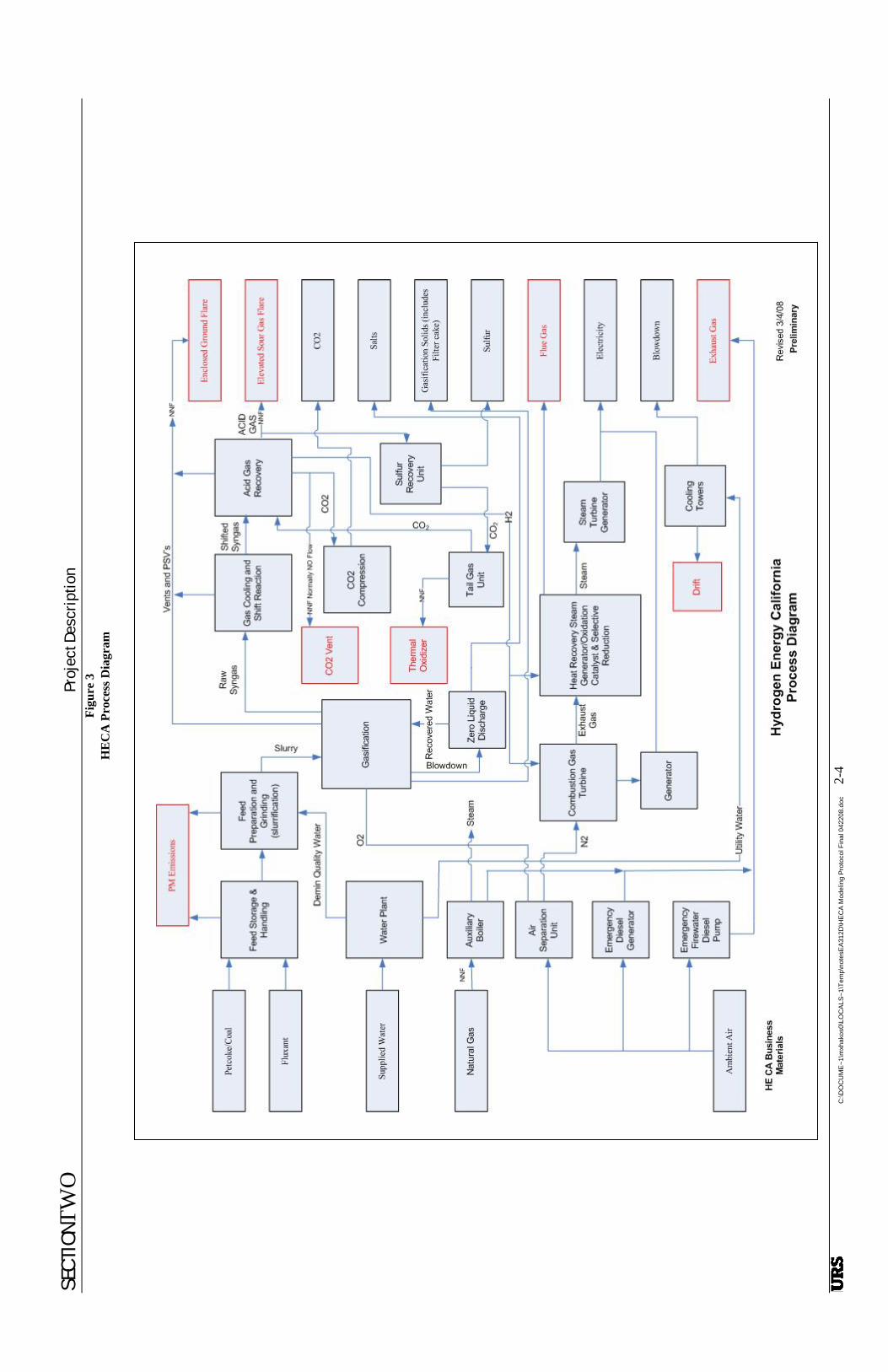
Figure 2 shows the preliminary layout of the proposed power plant, including property lines and the locations of all major equipment. The process diagram of the project is shown in Figure 3. Emission points are identified on Figure 2 by number and shown in the legend. These numbers are used in the discussions below.
The proposed power generation facility (power block) will consist of one GE Model 7FB or equivalent Siemens CTG with an ISO base load gross output of approximately 230 MW. The CTG will be designed and constructed to burn multiple fuels (i.e., a combination of fuels ranging from hydrogen to pipeline-quality natural gas and mixtures of the two) with an evaporative cooling system installed on the inlet air for use when the ambient temperatures exceed 59°F. The CTG will be followed by a Heat Recovery Steam Generator (HRSG). The HRGS will also be designed to burn the same multiple fuels as the CTG. The maximum fuel flow rate for the CTG and HRSG will be approximately 1,850 MMBtu/hr and 500 MMBtu/hr (higher heating value, HHV), respectively. Exhaust from the CTG/HRSG will exit through a stack with a height of 160 feet (Emission Point No. 4).
An air/nitrogen mixture is supplied to the CTG through an inlet air filter, inlet air evaporative cooling system, compressor section of the combustion turbine and then exits through the compressor discharge casing to the combustion chambers. Fuel is also supplied to the combustion chambers where it is ignited with the compressed air/nitrogen mixture, expanding through the turbine blades, driving the turbine, electricity generator, and the CTG compressor. Exhaust gas from the CTG is directed through internally insulated ductwork to the HRSG. Steam generated in the HRSG is admitted to a steam turbine generator (STG) for electric power generation. The STG system, rated at approximately 150 MW consists of a steam turbine, gland steam system, lube oil system, hydraulic control system, and a hydrogen cooled generator with all required accessories.
A diffusion combustor system using nitrogen as a diluent when firing hydrogen and using steam as a diluent when firing natural gas will be used to control the NOX emissions from the CTG. A selective catalytic reduction (SCR) system will be provided in the HRSG to further reduce the NOX emissions to the atmosphere. The SCR system for the HRSG will inject aqueous ammonia into the exhaust gas stream upstream of a catalyst bed to reduce NOX to inert nitrogen and water. An oxidation catalyst system will also be incorporated into the air quality control system to control emissions of CO and ROGs.
The auxiliary CTG will be fired exclusively on natural gas and will be equipped with water injection and selective catalytic reduction (SCR) for the control of NOx emissions and an oxidation catalyst for control emissions of CO and ROGs. The auxiliary CTG will operate in simple cycle mode and will have an

SECTIONTWO Project Description
C:\DOCUME~1\mxhakos0\LOCALS~1\Temp\notesEA312D\HECA Modeling Protocol Final 042208.doc 2-2
exhaust stack with a height of 90 feet. (Emission Point No. X). The auxiliary CTG will be added to the plot plan and the process diagram in their next revision.
An auxiliary boiler (Emission Point No. 6) will provide steam to facilitate CTG startup and for other purposes. The auxiliary boiler will be designed to burn a single fuel (i.e., pipeline-quality natural gas) at the design maximum fuel flow rate of 100 MMBtu/hr HHV. The auxiliary boiler will be equipped with ultra-low NOX combustors and will have an estimated annual capacity of 25 percent.
HECA will also incorporate a thermal oxidizer (Emission Point No. 7) on the tail gas treatment (TGT) unit to control emissions during startup of the TGT unit. After the TGT unit is started, emissions from the TGT thermal oxidizer will cease being emitted and will be returned to the process. An enclosed ground flare (Emission Point No. 10) will be used during gasifier startup and an elevated flare (Emission Point No. 9) will be used to oxidize releases of system overpressure. Each of the three gasification trains will have one natural-gas fired burner used to keep the gasification train in hot standby mode (Emission Point Nos. 11a -11c). These burners will not operate when the gasification train is operating.
A 16-celled mechanical draft cooling tower (Emission Point No. 2) will be installed to perform the required cooling for the CTGs, STG, and associated equipment. Other sources of emissions will include a 4-celled mechanical draft cooling tower for the air separation unit (Emission Point No. 1), diesel-fired internal combustion engine drivers for an emergency fire pump rated at about 550 horsepower (Emission Point No. 5), and two 1 MW each emergency generators (Emission Point No. 3).
A CO2 vent stack (Emission Point No. 8) will provide an alternative operating scenario for releasing the produced CO2 when the CO2 injection system is unavailable. The CO2 vent will enable HECA to operate for brief periods rather than be disabled by a gasifier shutdown and subsequent gasifier restart. The CO2 vent exhaust stream will be nearly all CO2, with small amounts of CO and Hydrogen Sulfide (H2S).
In addition to the sources above, there will be emissions of PM10 from feedstock and gasifier solids materials handling operations. These operations include bulk material unloading, loading, belt conveying, belt transfer points, silo loading and reclaim.

SECT
IONT
WO
Pr
ojec
t Des
crip
tion
C
:\DO
CU
ME
~1\m
xhak
os0\
LOC
ALS
~1\T
emp\
note
sEA
312D
\HE
CA
Mod
elin
g P
roto
col F
inal
042
208.
doc
2-3
Figu
re 2
H
EC
A F
acili
ty P
lot P
lan
and
Fenc
elin
e

SECT
IONT
WO
Pr
ojec
t Des
crip
tion
C
:\DO
CU
ME
~1\m
xhak
os0\
LOC
ALS
~1\T
emp\
note
sEA
312D
\HE
CA
Mod
elin
g P
roto
col F
inal
042
208.
doc
2-4
Figu
re 3
H
EC
A P
roce
ss D
iagr
am


SECTIONTHREE Regulatory Setting
C:\DOCUME~1\mxhakos0\LOCALS~1\Temp\notesEA312D\HECA Modeling Protocol Final 042208.doc 3-1
SECTION 3 REGULATORY SETTING
3.1 CALIFORNIA ENERGY COMMISSION REQUIREMENTS
For projects with electrical power generation capacity greater than 50 MW, CEC requires that applicants prepare a comprehensive Application for Certification (AFC) document addressing the proposed project’s environmental and engineering features. An AFC must include the following air quality information (CEC, 1997):
• A description of the project, including project emissions of air pollutants and greenhouse gases, fuel type(s), control technologies and stack characteristics;
• The basis for all emission estimates and/or calculations;
• An analysis of Best Available Control Technology (BACT) according to San Joaquin Valley Air Pollution Control District (SJVAPCD) Rules;
• Existing baseline air quality data for all regulated pollutants;
• Existing meteorological data, including temperature, wind speed and direction, and mixing height;
• A listing of applicable laws, ordinances, regulations, standards (LORS), and a determination of compliance with all applicable LORS;
• An emissions offset strategy;
• An air quality impact assessment (i.e., national and state ambient air quality standards [AAQS] and PSD review) and protocol for the assessment of cumulative impacts of the proposed project along with permitted and under construction projects within a 10 km radius; and
• An analysis of human exposure to air toxics (i.e., health risk assessment [HRA]).
For HECA, the air quality impact assessment, the cumulative impacts assessment, and the HRA will be performed using dispersion models.
3.2 SAN JOAQUIN VALLEY AIR POLLUTION CONTROL DISTRICT REQUIREMENTS
The SJVAPCD has promulgated NSR requirements under Rule 2201. In general, all equipment with the potential to emit air pollutants is subject to the requirements of this rule, which has the following major requirements that potentially apply to new sources such as HECA:
• Installation of BACT,
• Ambient air quality impact modeling to demonstrate compliance with NAAQS and CAAQS and to evaluate impacts to plume visibility in Class I areas near the proposed source(s),
• Emission offsets,
• Statewide compliance for all applicant-owned or operated facilities in California,

SECTIONTHREE Regulatory Setting
C:\DOCUME~1\mxhakos0\LOCALS~1\Temp\notesEA312D\HECA Modeling Protocol Final 042208.doc 3-2
Assembly Bill 2588, California Air Toxics Hot Spots Program and SJVAPCD Rule 3110 establish allowable incremental health risks for new or modified sources of toxic air contaminant (TAC) emissions This rule specifies limits for maximum individual cancer risk (MICR), cancer burden, and non-carcinogenic acute and chronic hazard indices (HI) for new or modified sources of TAC emissions. The health risks resulting from project emissions, as demonstrated by means of an approved health risk assessment, must not exceed established threshold values.
3.3 U.S. ENVIRONMENTAL PROTECTION AGENCY REQUIREMENTS
USEPA has promulgated PSD regulations applicable to new Major Sources and Major Modifications to existing Major Sources. HECA will be a Major Source because it is a fossil-fuel fired steam electric plant of more than 250 MMBtu/hr heat input and will have the potential to emit more than 100 tpy of NOx, and CO. Many of the PSD requirements are the same as the AFC and SJVAPCD Rule 2201 requirements described above (e.g., project description, BACT, ambient air quality standards analysis). However, PSD requires the following additional analyses:
• An analysis of the potential impacts from the new emissions from HECA relative to PSD Significant Impact Levels (SILs) and PSD Increments;
• An analysis of air quality related values (AQRV) to ensure the protection of visibility in federal Class I National Parks and National Wilderness Areas within 100 km of the proposed project;
• An evaluation of potential impacts on soils and vegetation of commercial and recreational value; and
• An evaluation of potential growth-inducing impacts.

Air Quality Impact Analysis SECTIONFOUR For Class II Areas
C:\DOCUME~1\mxhakos0\LOCALS~1\Temp\notesEA312D\HECA Modeling Protocol Final 042208.doc 4-1
SECTION 4 AIR QUALITY IMPACT ANALYSIS FOR CLASS II AREAS
This section describes the dispersion models and modeling techniques that will be used in performing the near-field criteria pollutant impact analysis for HECA. The objectives of the modeling are to demonstrate that air emissions from HECA will not cause incremental impacts that exceed the Class II PSD Significant Impact Levels (SILs), nor contribute to exceedances of state and federal ambient air quality standards.
In November 2005, the USEPA officially recognized the American Meteorological Society/ Environmental Protection Agency Regulatory Model (AERMOD) as the preferred dispersion model for regulatory applications, replacing the Industrial Source Complex Short Term 3 (ISCST3) model. Also, both CEC staff recommendations and the SJVAPCD guidance for air dispersion modeling (SJVAPCD, 2006) support the use of AERMOD for power plant licensing/permitting analyses. Accordingly, AERMOD (Version 07026) will be used for the dispersion modeling associated with HECA.
4.1 TURBINE SCREENING MODELING
An initial screening modeling analysis will be conducted to determine the turbine stack parameters for the most important project source, i.e., the CTG/HRSG that correspond to maximum ground-level pollutant concentrations. This information will be obtained by running a series of AERMOD simulations with the full meteorological input data set (see Section 4.6) with source inputs representing a range of different load conditions and ambient temperatures. The stack parameters that align with the highest offsite impact from these sources for each pollutant and averaging time period will be used in the subsequent refined modeling simulations.
4.2 REFINED MODELING
The purpose of the refined modeling analysis is to demonstrate that air emissions from HECA will not cause or contribute to an ambient air quality violation. The AERMOD model (version 07026) will be used for the refined modeling of criteria pollutants. Specific modeling procedures that will be used for evaluating project impacts versus the state and federal ambient air quality standards, PSD significance thresholds and applicable health risk criteria are discussed below. Table 4-1 shows the regulatory criteria that will be used to evaluate the significance of predicted pollutant concentrations.
Analysis of land uses adjacent to HECA was conducted in accordance with Section 8.2.8 of the Guideline on Air Quality Models (EPA-450/2-78-027R and Auer [1978]), EPA AERMOD implementation guide (2004), and its addendum (2006).
Based on the Auer land use procedure, more than 50 percent of the area within a 3-km radius of HECA power plant is classified as rural. Since the Auer classification scheme requires more than 50 percent of the area within the 3-km radius around a proposed new source to be non-rural for an urban classification, the rural mode will be used in the AERMOD modeling analyses. All regulatory default options will be used, including building and stack tip downwash, default wind speed profiles, exclusion of deposition and gravitational settling, consideration of buoyant plume rise, and complex terrain.

Air Quality Impact Analysis SECTIONFOUR For Class II Areas
C:\DOCUME~1\mxhakos0\LOCALS~1\Temp\notesEA312D\HECA Modeling Protocol Final 042208.doc 4-2
Table 4-1 Relevant Ambient Air Quality Standards and Significance Levels
PSD Increments (µg/m3) Pollutant Averaging
Time CAAQS
(a, b) NAAQS
(b, c)
PSD Class II Significance
Impact Levels (µg/m3)
PSD Significant Emission Rates
(tpy) Class I Class II
8-hour 9.0 ppm (10,000 µg/m3)
9.0 ppm (10,000 µg/m3) 500
CO 1-hour 20 ppm
(23,000 µg/m3) 35 ppm
(40,000 µg/m3) 2,000 100
Annual 0.030 ppm (57 µg/m3)
0.053 ppm (100 µg/m3) 1 2.5 25
NO2(d)
1-hour 0.18 ppm (339 µg/m3)
40
Annual 0.03 ppm (80 µg/m3) 1 2 20
24-hour 0.04 ppm(e) (105 µg/m3)
0.14 ppm (365 µg/m3) 5 5 91
3-hour 0.5 ppm
(1,300 µg/m3) 25 25 512
SO2
1-hour 0.25 ppm
(655 µg/m3)
40
Annual 20 µg/m3 See footnote(e) 1 4 17 PM10
24-hour 50 µg/m3 150 µg/m3 5 15
8 30
Annual 12 µg/m3 15 µg/m3 PM2.5
24-hour 35 µg/m3
8-hour 0.07 ppm (137 µg/m3)
0.075 ppm (147 µg/m3) See footnote(f)
O3 1-hour 0.09 ppm
(180 µg/m3) See footnote(g)
H2S 1-hour 0.03 ppm(h) Notes: a. California standards for ozone (as volatile organic compound), carbon monoxide, sulfur dioxide (1-hour), nitrogen dioxide, and PM10, are values that are
not to be exceeded. The visibility standard is not to be equaled or exceeded. b. Concentrations are expressed first in units in which they were promulgated. Equivalent units are given in parentheses and based on a reference
temperature of 25°C and a reference pressure of 760 mm of mercury. All measurements of air quality area to be corrected to a reference temperature of 25°C and a reference pressure of 760 mm of mercury (1,013.2 millibars).
c. National standards, other than those for ozone and based on annual averages, are not to be exceeded more than once a year. The ozone standard is attained when the expected number of days per calendar year with maximum hourly average concentrations above the standard is ≤ 1.
d. NO2 is the compound regulated as a criteria pollutant; however, emissions are usually based on the sum of all NOx. e. The federal annual PM10 standard was revoked by USEPA on October 17, 2006. f. Modeling is required for any net increase of 100 tons per year or more of ROC subject to PSD. g. New federal 8-hour ozone and fine particulate matter (PM2.5) standards were promulgated by USEPA on July 18, 1997. The federal 1-hour ozone
standard was revoked by USEPA on June 15, 2005.
h. The Hydrogen Sulfide ambient air quality standard is an odor based threshold instead of health based.

Air Quality Impact Analysis SECTIONFOUR For Class II Areas
C:\DOCUME~1\mxhakos0\LOCALS~1\Temp\notesEA312D\HECA Modeling Protocol Final 042208.doc 4-3
4.2.1 PSD Modeling Analyses
As the proposed project will trigger PSD as a Major Source, modeling will be required to determine whether its incremental impacts on ambient levels of attainment pollutants (NO2, SO2 and CO) will exceed Class II significant impact levels, or SILs. If these SILs were predicted to be exceeded, then an analysis of increment consumption due to all new sources that commenced operation since the local PSD baseline date would be required. However, it is anticipated that the increased emissions of these pollutants due to HECA will not cause incremental effects above the federal SILs.
4.2.2 Ambient Air Quality Standards Analysis
Compliance with the SJVAPCD Rule 2201 modeling requirements for attainment pollutants will be demonstrated by modeling the maximum ground-level concentrations of the proposed Project at any receptor and adding conservative background concentrations, based on recent data from the most representative SJVAPCD air quality monitoring station. HECA will not be considered to cause or contribute to a near-field ambient air quality violation unless impacts from these sources combined with the background concentration exceed the most stringent ambient air quality standard.
NO2 impact estimates for both the 1-hour and annual averaging times will be modeled by executing AERMOD with the USEPA ozone limiting method (OLM) option for both hourly and annual impacts.
Note that emissions reduction credits will be obtained by the applicant to offset Project emissions increases of all non-attainment pollutants and their precursors, i.e. NOx, ROG, PM10 and SO2 that are above the SJVAPCD offset triggering levels specified in the Districts Rule 2201.4.5.3.
4.2.3 Health Risk Assessment Analysis
Both CEC and SJVAPCD require a health risk assessment (HRA) to evaluate potential health effects of TAC emissions from the operation of the project. Contaminants emitted by the project with potential carcinogenic effects or chronic and/or acute non-carcinogenic effects will be considered. This health risk assessment will be performed following the Office of Environmental Health Hazard Assessment (OEHHA), Air Toxics Hot Spots Program Risk Assessment Guidelines (OEHHA, 2003). As recommended by the Guidelines, the California Air Resources Board (CARB) Hotspots Analysis and Reporting Program (HARP) (CARB, 2005) will be used to perform an OEHHA Tier 1 health risk assessment for the project. HARP includes two modules: a dispersion module and a risk module. The HARP dispersion module incorporates the USEPA ISCST3 air dispersion model, and the HARP risk module implements the latest Risk Assessment Guidelines developed by OEHHA. For consistency with the criteria pollutant modeling, the dispersion modeling will be conducted with AERMOD. ARB has created a beta version software package, HARP File Converter, to convert AERMOD dispersion results into a format that can be read into the HARP risk module. Thus HARP with AERMOD will be used for this HRA.

Air Quality Impact Analysis SECTIONFOUR For Class II Areas
C:\DOCUME~1\mxhakos0\LOCALS~1\Temp\notesEA312D\HECA Modeling Protocol Final 042208.doc 4-4
First, ground-level concentrations from HECA emissions will be estimated using the AERMOD dispersion model. The dispersion modeling analysis will be consistent with, and use input parameters that are similar to those discussed above for the criteria pollutant analyses using AERMOD. The same five-year Bakersfield meteorological data set that will be used for the criteria pollutant air quality impact assessment will also be used in the HRA. The maximum 1-hour and annual impacts determined by AERMOD will be used in the HARP model to estimate the corresponding health risks. Receptor spacing will be the same as for the criteria pollutant modeling described later in this Protocol. The HARP simulations will also include the census receptors out to 10 km, and additional receptors will be placed at all sensitive locations (e.g., schools, hospitals, etc.) out to a distance of 5 km (3 miles). Receptors will also be placed at all nearby residents.
Incremental cancer risk will be estimated using the “Derived (Adjusted)” calculation method in HARP. For the calculation of cancer risk, the duration of exposure to project emissions will be assumed to be 24 hours per day, 365 days per year, for 70 years, at all receptors. Chronic non-cancer risks will be calculated by means of the “Derived (OEHHA)” method. No bodies of water are near HECA , thus fish ingestion and drinking water consumption pathways will not be included in this analysis.
The HRA performed by means of the HARP model will follow the following steps:
• Define the location of the maximally exposed individual (MEI) (i.e., the location where the highest carcinogenic risk may occur);
• Define the locations of the maximum chronic non-carcinogenic health effects and the maximum acute health effects;
• Calculate concentrations and health effects at locations of maximum impact for each pollutant; and
• Calculate cancer burden if the maximum cancer risk is predicted to be greater than one in a million.
4.3 MODELING EMISSIONS INVENTORY
4.3.1 Operational Project Sources
Operational emissions from the project will be dominated by the CTG with HRSG. Conceptual plant design includes SCR for NOx and oxidation catalysts for CO that will comply with recent BACT determinations for similar IGCC projects recently permitted in United States. Emissions of SO2 and PM10 will be maintained at low levels, owing to HECA commitment to have SO2 and PM10 emissions comparable to a similarly sized integrated gasification combined cycle power plant having exclusive use of hydrogen as fuel for the gas turbine. Table 4-2 summarizes the estimated annual emissions from the main project sources for each criteria pollutant. The CTG and HRSG emissions estimates reflect the assumed operating hours and numbers of turbine startups described in Section 1.1. Table 4-2 does not include the small contributions to project emissions that will come from the one emergency diesel generator and the one emergency firewater pump engine, or the startup emissions from the thermal oxidizer and the two flares. The engines will normally be operated only a few hours per year in order to test their operability in the event of an emergency situation. The thermal oxidizer and the two flares will

Air Quality Impact Analysis SECTIONFOUR For Class II Areas
C:\DOCUME~1\mxhakos0\LOCALS~1\Temp\notesEA312D\HECA Modeling Protocol Final 042208.doc 4-5
have only pilot flame emissions during normal operation. However, emissions from these engines, the thermal oxidizer and the two flares will be included in the dispersion modeling conducted for HECA.

Air Quality Impact Analysis SECTIONFOUR For Class II Areas
C:\DOCUME~1\mxhakos0\LOCALS~1\Temp\notesEA312D\HECA Modeling Protocol Final 042208.doc 4-6
Table 4-2 Approximate Annual Pollutant Emissions for HECA Turbine/HRSG, Auxiliary CTG, Auxiliary
Boiler, and the Cooling Towers at Steady State Operation
Pollutant Annual Emissions (tpy)
Turbine/HRSG Auxiliary CTG Auxiliary Boiler
Cooling Towers Total HECA Emission Approximation *
NOx 215 17 2 0 ~ 250 CO 140 28 6 0 > 250 SO2 30 5 <1 0 <50 PM10 160 21 <1 25 < 250 VOC 35 5 <1 0 <50 Note: * Total HECA emission approximations include bulk materials handling dust emissions and fixed duration events such as startups and shutdown
4.3.2 Project Construction Sources
Temporary construction emissions will result from heavy equipment exhaust (primarily NOx and diesel particulate emissions) and fugitive dust (PM10) from earthmoving activities and vehicle traffic on paved and unpaved surfaces. A detailed Excel Workbook will be created to estimate criteria pollutant emissions for non-overlapping phases of Project construction, based on information from the Project design engineers on the equipment use by month throughout the construction schedule and the area extent of ground disturbance that will occur during different construction phases. Depending on the magnitude of emissions for different pollutants and the proximity of construction activities to the property boundary for each phase, one or more emission scenarios representing reasonable worst-case equipment activity and ground disturbance for each averaging time will be selected for subsequent dispersion modeling to ensure that maximum off-site air quality impacts due to these temporary activities will be assessed. The selected emissions scenarios will be modeled using AERMOD with the same near-field receptor grids and the same meteorological input data used for the modeling of the Project’s operational emissions. Fugitive dust emissions from the construction site, including the corridors for new transmission lines, gas lines or water pipelines, parking areas and lay-down areas will be modeled as area or volume sources. Equipment exhaust emissions of gaseous pollutants and particulates will be modeled as a series of point sources distributed over the site and linears corridors, as appropriate. Ultra-low sulfur diesel fuel (15 ppm by weight or less) will be utilized on any emission calculations for construction equipment used at HECA site.
4.3.3 Toxic Air Contaminant Sources
TACs will also be emitted from the operational HECA project due to combustion of natural gas, hydrogen gas and diesel fuels. Only small quantities of TACs will be emitted from these sources - primarily benzene, formaldehyde, and polycyclic aromatic hydrocarbons, when natural gas will be used as fuel for the CTG/HRSG train and the auxiliary boiler. Two new diesel-fired engines are proposed as part of the project. These include one fire pump engine and two standby emergency generator engine drivers. Emission estimates for TACs from these sources will be based on diesel particulate mater (DPM)

Air Quality Impact Analysis SECTIONFOUR For Class II Areas
C:\DOCUME~1\mxhakos0\LOCALS~1\Temp\notesEA312D\HECA Modeling Protocol Final 042208.doc 4-7
emission factors obtained from standard SJVAPCD, CARB and EPA factors and/or vendor data, if available. The cooling towers’ TAC emissions will be estimated using cooling tower feedwater quality data and drift calculations. Emissions of TACs from the CTG/HRSG train when hydrogen is being used and from the flares and the tailgas incinerator during periods of startup and shutdown will be estimated using a combination of emission factors, inventories from other IGCC facilities and vendor data, if available.
4.3.4 Cumulative Impact Analysis Including Off-Property Sources
A cumulative modeling analyses will be performed using AERMOD to evaluate the combined impacts of HECA Project emissions increases with those of any other new sources within 10 km (6 miles) from HECA that are currently either under construction, undergoing permitting or expected to be permitted in the near future. Requests will be made to the SJVAPCD, Kern County Planning Department, the City of Bakersfield, and adjacent cities to request information that will be used to develop lists of all such new or planned emission sources. When received, these lists will be forwarded to CEC for review. Based on this information, and the CEC response, additional sources may be included in the cumulative source modeling analysis. However, because of the relative remoteness and rural nature of the project site area, few recent new sources are expected to be identified.
4.4 BUILDING WAKE EFFECTS
The effect of building wakes (i.e., downwash) upon the stack plumes of emission sources at the facility will be evaluated in accordance with USEPA guidance (USEPA, 1985). Direction-specific building data will be generated for stacks below good engineering practice (GEP) stack height using the most recent version of USEPA Building Parameter Input Program – Prime (BPIP-Prime). Appropriate information will be provided in the AFC and other permit applications that describe the input assumptions and output results from the BPIP-Prime model.
4.5 RECEPTOR GRID
The receptor grids that will be used in the AERMOD modeling analyses described in this Protocol for operational sources will be as follows:
• 25-m spacing along the fenceline and extending from the fenceline out to 100 m beyond the property line;
• 50-m spacing from 100 to 250 m beyond the property line;
• 100-m spacing from 250 to 500 m beyond the property line;
• 250-m spacing from 500 m to 1 km beyond the property line;
• 500-m spacing within 1 to 2 km of project sources; and
• 1,000-m spacing within 2 to 10 km of project sources.
During the refined modeling analysis for operational Project emissions, if a maximum predicted concentration for a particular pollutant and averaging time is located within the portion of the receptor

Air Quality Impact Analysis SECTIONFOUR For Class II Areas
C:\DOCUME~1\mxhakos0\LOCALS~1\Temp\notesEA312D\HECA Modeling Protocol Final 042208.doc 4-8
grid with spacing greater than 25 m, a supplemental dense receptor grid will be placed around the original maximum concentration point and the model will be rerun. The dense grid will use 25-m spacing and will extend to the next grid point in all directions from the original point of maximum concentration.
Due to the large computation time required to run AERMOD, this receptor grid, with the additional dense nested grid points, was determined to best balance the need to predict maximum pollutant concentrations and allow the all operational modeling runs to be completed in less than one week.
Because construction emission sources release pollutants to the atmosphere from small equipment exhaust stacks or from soil disturbances at ground level, maximum predicted construction impacts for all pollutants and averaging times will occur within the first kilometer from the HECA site boundary. Accordingly, only the portion of the above grid with 25 m spacing out to a distance of 1 km will be used for the construction modeling.
The same receptor grid used in the criteria pollutant modeling for the operational project will be used in the HRA modeling, with additional receptors placed at all sensitive locations (e.g., schools, hospitals, etc.) out to 5 km (3 miles). Census receptors out to 10 km will also be included in the populated areas nearest to the proposed HECA facility. Finally, discrete receptors will be placed at the locations of all nearby residences.
A detailed project map and a 7 ½- minute U.S Geological Survey (USGS) map will be provided in the AFC showing the locations of the grid receptors. Actual Universal Transverse Mercator (UTM) coordinates will be used. The CAAQS and NAAQS apply to all locations outside the applicant’s facility, i.e. everywhere where public access is not under the control of the applicant. Therefore, the fenceline will be placed along the facility’s property boundary, and the receptors will be placed on and outside of the fenceline.
4.6 METEOROLOGICAL AND AIR QUALITY DATA
4.6.1 Meteorological Data
Meteorological data suitable for direct input to AERMOD were obtained from the SJVAPCD website. Hourly surface data for calendar years 2000, 2001, 2002, 2003, and 2004 were obtained from the SJVAPCD for the Bakersfield Airport meteorological station which is located, in the City of Bakersfield approximately 32.2 km (20 miles) ENE of the HECA site. These data have been pre-processed by the SJVAPCD with the Oakland upper air data to create an input data set specifically tailored for input to AERMOD.
The meteorological data recorded at Bakersfield Airport are acceptable for use at HECA facility for two reasons, proximity and terrain similarity. The terrain immediately surrounding the Project site can be categorized as a fairly flat, or gradually sloping rural area in an area with developed oil wells. The terrain around the Bakersfield Airport also consists of relatively flat, or gradually sloping rural or suburban areas. Thus the land use and the location with respect to near-field terrain features are similar. Additionally, there are no significant terrain features separating the Bakersfield Airport from the HECA facility site that would cause significant differences in wind or temperature conditions between these respective areas. Therefore the five years of meteorological data selected from the Bakersfield Airport were determined to

Air Quality Impact Analysis SECTIONFOUR For Class II Areas
C:\DOCUME~1\mxhakos0\LOCALS~1\Temp\notesEA312D\HECA Modeling Protocol Final 042208.doc 4-9
be representative for purposes of evaluating the Project’s air quality impacts. The Bakersfield Airport is the closest full-time meteorological recording station to the HECA facility site, and thus meteorological conditions at the sites will be very similar.
Seasonal and annual wind roses based on the five years of Bakersfield Airport surface meteorological data are provided as Appendix A to this Protocol. Winds for all seasons and all years blow predominantly from the sector between northwest and north, although the directional pattern is more variable during the fall and winter seasons.
4.6.2 Air Quality Monitoring Data
Air quality monitoring data to represent existing air quality in the Project area were obtained from the USEPA AirData (2006) and the CARB-California Air Quality Data website (2006). The most recent three years of data (2004-2006) from the Taft-College, Shafter, Bakersfield Golden State Highway, and Bakersfield 5558 California Avenue monitoring stations were collected to determine the most representative baseline concentrations for each air pollutant and averaging period addressed in the California and National ambient air quality standards. The maximum concentration recorded at these monitoring stations over the three-year period will be used as a conservative representation of existing air quality condition at the proposed Project site.
The Taft-College monitoring station is located approximately 20 km to the south of the HECA facility site. The Taft-College station only monitors PM10, and TSP (until 2005). The Bakersfield Golden Highway station is the closest station that monitors all the criteria pollutants, except SO2, and is located approximately 39 km to the east of the HECA facility site. The Bakersfield 5558 California Avenue station also measures all pollutants except CO and SO2. This station is located about 34 km east of the HECA site. The only station in the San Joaquin Valley Air Basin that monitors SO2 is the CARB station at First Street in Fresno, located approximately 160 km (100 miles) to the north. SO2 data have only been recorded in Fresno County for one of the last nine years (2003), a practice that is justified by the low levels that have been recorded for this pollutant when measurements have been made.
The selected maximum baseline concentrations for all pollutants are summarized in Table 4-3. These data will be added to the modeled maximum impacts due to project emissions for each pollutant and averaging time, and the totals will then be compared with the applicable AAQS. This is a conservative approach because it assumes that the highest recorded background values and the modeled maximum impacts occur at the same time and location for each pollutant and averaging time, a highly unlikely scenario. Note that the maximum background concentrations of PM10 and PM2.5 in the project area currently exceed the corresponding CAAQS and NAAQS.

Air Quality Impact Analysis SECTIONFOUR For Class II Areas
C:\DOCUME~1\mxhakos0\LOCALS~1\Temp\notesEA312D\HECA Modeling Protocol Final 042208.doc 4-10
Table 4-3 Highest Monitored Pollutant Concentrations Near the Proposed HECA Site (2004 – 2006)
Pollutant Averaging Time Highest Monitoring Concentration Monitoring Station Address Year
8-hour 2.6 ppm (2,889 µg/m3) Bakersfield Golden State Highway 2004 CO
1-hour 4.1 ppm (4,715 µg/m3) Bakersfield Golden State Highway 2004
Annual 0.019 ppm (35.8 µg/m3) Shafter 2006 NO2
1-hour 0.100 ppm (188.2 µg/m3) Shafter 2006
Annual 0.002 ppm (5.33 µg/m3) Fresno Fremont School 2003
24-hour 0.004 ppm (10.5 µg/m3) Fresno Fremont School 2003
3-hour 0.006 ppm (15.6 µg/m3) Fresno Fremont School 2003 SO2
1-hour 0.009 ppm (23.58 µg/m3) Fresno Fremont School 2003
Annual 48.5 µg/m3 Bakersfield 5558 California Avenue 2006 PM10a (Non-attainment area) 24-hour 159.0 µg/m3 c Bakersfield 5558 California Avenue 2006
Annual 22.4 µg/m3 Bakersfield 5558 California Avenue 2005 PM2.5 b (Non-attainment area) 24-hour 102.1 µg/m3 Bakersfield 5558 California Avenue 2005
Source: CARB ADAM website (Last access: January, 2008). a Although EPA has determined that the San Joaquin Valley Air Basin has attained the federal PM 10 standards, their determination does not constitute a redesignation to attainment per section 107(d)(3) of the Federal Clean Air Act. The Valley will continue to be designated nonattainment until all of the Section 107(d)(3) requirements are met. This area will be treated as the federal PM 10 non-attainment area until future redesignation. b The Valley is designated nonattainment for the 1997 PM 2.5 federal standards. EPA designations for the 2006 PM 2.5 standards will be finalized in December 2009. The District has determined, as of the 2004-06 PM 2.5 data, that the Valley has attained the 1997 24-Hour PM 2.5 standard. . This area will be treated as the federal PM 2.5 non-attainment area until future redesignation. c An exceedance is not necessarily a violation.
4.7 FUMIGATION MODELING
Fumigation can occur when a stable layer of air lies a short distance above the release point of a plume and unstable air lies below. Especially on sunny mornings with light winds, the heating of the earth’s surface causes a layer of turbulence, which grows in depth over time and may intersect an elevated exhaust plume. The transition from stable to unstable surroundings can rapidly draw a plume down to ground level and create relatively high pollutant concentrations for a short period. Typically, a fumigation analysis is conducted using the USEPA model SCREEN3 when the project site is rural and the stack height is greater than 10 m.
A fumigation analysis will be performed using SCREEN3 to calculate concentrations from inversion breakup fumigation; no shoreline fumigation modeling will be performed for the HECA location. A unit emission rate will be used (1 gram per second) in the fumigation modeling simulations to represent the plant emissions, and the model results will be scaled to reflect expected plant emissions for each pollutant. Inversion breakup fumigation concentrations will be calculated for 1- and 3-hour averaging times using USEPA-approved conversion factors. These multiple-hour model predictions are

Air Quality Impact Analysis SECTIONFOUR For Class II Areas
C:\DOCUME~1\mxhakos0\LOCALS~1\Temp\notesEA312D\HECA Modeling Protocol Final 042208.doc 4-11
conservative, since inversion breakup fumigation is a transitory condition that would most likely affect a given receptor location for only a few minutes at a time.


Air Quality Impact Analysis
SECTIONFIVE For Class I Areas
C:\DOCUME~1\mxhakos0\LOCALS~1\Temp\notesEA312D\HECA Modeling Protocol Final 042208.doc 5-1
SECTION 5 AIR QUALITY IMPACT ANALYSIS FOR CLASS I AREAS
An evaluation of potential impacts in Class I areas within 100 km of the HECA site will be conducted, because HECA’s potential emissions increases of some pollutants will be sufficiently high to be considered a Major Source, thus triggering the federal PSD program. A Major Source must evaluate impacts to visibility and other air quality related values (AQRV) at all Class I areas that are located within a 100-km radius of the facility. All pollutants for which Project emissions are above the Major Source threshold (in this case, 100 tpy) and all pollutants for which emissions are above the PSD Significant Emissions Rates must be evaluated. This section describes the dispersion models and modeling techniques that will be used in performing the Class I area air quality analyses for HECA. The objectives of the modeling are to demonstrate whether air emissions from HECA would cause or contribute to a PSD increment exceedance or cause a significant impact on visibility, regional haze or sulfur or nitrogen deposition in any Class I area.
Three Class I areas are located within the region of the HECA site and require further evaluation: Dome Land Wilderness Area, Sequoia National Park, and San Rafael Wilderness Area. However, detailed review of the locations of these Class I areas relative to the HECA site shows that Dome Land Wilderness Area and Sequoia National Park are greater than 100 km from HECA . Therefore, these two Class I areas do not meet the criterion of being within 100 km and will not be included in the HECA analysis. The nearest parts of the San Rafael Wilderness are located beyond 50 km and within 100 km from the proposed facility, thus only this Class I area and only far-field AQRV analyses will need to be completed. The CALMET/CALPUFF (full-CALPUFF) model will be used to evaluate potential impacts in the far-field Class I area, including potential air quality impacts, sulfur and nitrogen deposition, and impacts to visibility.
Figure 3 shows the locations of the Class I areas relative to the proposed site for HECA and Table 5-1 lists the distances from HECA to the closest and farthest points in each Class I area. Figure 3 also shows the domain to be used for CALPUFF modeling of the San Rafael Wilderness Area (indicated by the blue rectangle). The federal authority in charge of the two Wilderness Areas is the United States Forest Service (USFS) and the National Park Service (NPS) has jurisdiction in Sequoia National Park. The AQRV analyses for the San Rafael Wilderness area will be conducted in a manner consistent with guidance from the NPS and USFS following the procedures set forth in the Federal Land Managers’ Air Quality Related Values Workgroup (FLAG) Phase I Report (USFS, 2000) and the Calpuff Reviewer’s Guideline (USFS and NPS, 2005).

Air Quality Impact Analysis
SECTIONFIVE For Class I Areas
C:\DOCUME~1\mxhakos0\LOCALS~1\Temp\notesEA312D\HECA Modeling Protocol Final 042208.doc 5-2
Table 5-1 Class I Areas Evaluated with Respect to 100-km Radius of the Proposed HECA Facility
Class I areas Distance from
HECA
(km)
Closest 110 Dome Land Wilderness Area Farthest 132
Closest 125 Sequoia National Park
Farthest 181 Closest 62 San Rafael Wilderness
Area Farthest 81

Air Quality Impact Analysis
SECTIONFIVE For Class I Areas
C:\DOCUME~1\mxhakos0\LOCALS~1\Temp\notesEA312D\HECA Modeling Protocol Final 042208.doc 5-3
Figure 4 Calpuff Domain and Receptor For the Class I Area Surrounding HECA

Air Quality Impact Analysis
SECTIONFIVE For Class I Areas
C:\DOCUME~1\mxhakos0\LOCALS~1\Temp\notesEA312D\HECA Modeling Protocol Final 042208.doc 5-4
The CALPUFF modeling domain selected for the modeling analyses will extend at least 50 km past the farthest edge in all directions from any of the Class I area being analyzed in order to reduce the probability that mass will be lost due to possible wind recirculation (Figure 3).
5.1 NEAR-FIELD CLASS I AREAS AIR QUALITY IMPACT ANALYSIS
There are no Class I Areas within 50 km of the proposed project location; therefore, no near field AQRV analyses are necessary.
5.2 FAR-FIELD CLASS I AREA AIR QUALITY IMPACT ANALYSIS: CALPUFF MODELING
To analyze potential impact of project emissions to visibility, PSD increment and sulfur and nitrogen deposition in the Class I area located within 100 km from the proposed project site, the CALPUFF model will be used in conjunction with the CALMET diagnostic meteorological model. CALPUFF is a transport and dispersion model that simulates the advection and dispersion of “puffs” of material emitted from modeled sources. CALPUFF can incorporate three-dimensionally varying wind fields, wet and dry deposition, and atmospheric gas and particle phase chemistry. The CALMET model is used to prepare the necessary gridded wind fields for use in the CALPUFF model. CALMET can also accept as input; mesoscale meteorological (MM5) data, surface station, upper air, precipitation, cloud cover, and over-water meteorological data (all in a variety of input formats). These data are merged and the effects of terrain and land cover types are simulated. This process results in the generation of gridded 3-dimensional wind fields that account for the effects of slope flows, terrain blocking effects, flow channeling, and spatially varying land uses.
The USEPA-approved regulatory air quality dispersion model CALPUFF (version 5.8) will be used for all far-field Class I area impact analyses. In addition, all supporting Version 5.8 editions of the pre- and post-processors will be used. Recommendations from the regulatory guidance documents listed below will be followed.
• Federal Land Managers Air Quality Related Values Workgroup (FLAG) Phase 1 Report. (USEPA December 2000),
• Interagency Workgroup on Air Quality Modeling (IWAQM), Phase 2 Summary Report and Recommendations for Modeling Long Range Transport Impacts. (USEPA December 1998), and
• Calpuff Reviewer’s Guide (Draft), (USFS and NPS, 2005).
Model options will be based on FLM guidance from the above documents and direct discussions with NPS and USFS air quality staff.
Copies of the model input and output files generated in the preparation of this and all other modeling analyses described in this Protocol will be provided with the final application.

Air Quality Impact Analysis
SECTIONFIVE For Class I Areas
C:\DOCUME~1\mxhakos0\LOCALS~1\Temp\notesEA312D\HECA Modeling Protocol Final 042208.doc 5-5
5.2.1 CALPUFF/CALMET Description
5.2.1.1 Location and Land-Use
The CALMET and CALPUFF models incorporate assumptions regarding land-use classification, leaf-area index, and surface roughness length to estimate deposition of emitted materials during atmospheric transport. U.S. Geological Survey (USGS) 1:250,000 scale digital elevation models (DEMs) and Land Use Land Cover (LULC) classification files will be used to develop the geophysical input files required by the CALMET model. Outputs of the terrain pre-processor (TERREL) and land use pre-processor (CTGPROC) will be combined in the geo-physical preprocessor (MAKEGEO) to prepare the CALMET geo-physical input file. The CALMET model will incorporate the necessary parameters in the CALMET output files for use in the CALPUFF model.
The CALPUFF modeling domain will extend from the HECA site 150 km to the west, 180 km to the north, 125 km to the east, and 150 km to the south. The grid-cells over this domain will be 4 km wide. The modeling domain will be specified using the Lambert Conformal Conic (LCC) projection system.
5.2.1.2 Meteorological Data
Pursuant to FLM guidance, a three-year meteorological data set will be developed using a combination of surface station and mesoscale meteorological (MM5) data for 2001-2003. Hourly CALMET data derived from the MM5 data for these three years will be obtained from the WRAP BART modeling for the Nevada-Utah domain. Surface meteorological, precipitation and ozone data will also be obtained from the WRAP BART modeling for the Nevada-Utah domain. No upper air stations will be used, since there are none within the domain shown in Figure 3 and the MM5 data provide a good first approximation of the vertical profile of the atmosphere.
CALMET wind fields will be generated using a combination of the MM5 data sets augmented with the surface data from the National Weather Service (NWS) stations described above. Per IWAQM guidance, the MM5 data will be interpolated to the CALMET fine-scale grid to create the “initial-guess” wind fields (IPROG = 14 for MM5).
5.2.1.3 Other Model Options
Size parameters for dry deposition of nitrate, sulfate, and PM10 particles will be based on default CALPUFF model options. Chemical parameters for gaseous dry deposition and wet scavenging coefficients will be based on default values presented in the CALPUFF User’s Guide. For the CALPUFF runs that incorporate deposition and chemical transformation rates (i.e. deposition and visibility), the full chemistry option of CALPUFF will be activated (MCHEM = 1). The nighttime loss for SO2, NOx and nitric acid (HNO3) will be set at 0.2 percent per hour, 2 percent per hour and 2 percent per hour, respectively. CALPUFF will also be configured to allow predictions of SO2, sulfate (SO4), NOx, HNO3, nitrate (NO3) and PM10 using the MESOPUFF II chemical transformation module.
Hourly ozone concentration files for the CALPUFF modeling will be obtained from the WRAP BART modeling data for the Nevada-Utah domain. Only data from the ozone monitoring stations within the HECA domain will be used.

Air Quality Impact Analysis
SECTIONFIVE For Class I Areas
C:\DOCUME~1\mxhakos0\LOCALS~1\Temp\notesEA312D\HECA Modeling Protocol Final 042208.doc 5-6
The background ammonia concentration will be set to 10 ppb, which is representative for a grassland or agricultural site, per the FLAG guidelines.
The regulatory default setting for MDISP=3 which utilizes the Pasquill-Gifford dispersion coefficients will be used in the CALPUFF modeling.
5.2.1.4 Receptors
Discrete receptors for the CALPUFF modeling within the San Rafael Wilderness Area will be obtained from the NPS Class One Area receptor database. No modifications to the receptor locations or heights provided in the database will be made. Latitude/Longitude coordinates of the Class I receptors will be converted to Lambert Conformal Conic (LCC) coordinates, based on the domain setup shown in CALMET options. These receptor points are shown in Figure 3.
5.2.2 Far-Field Class I Area Visibility and Regional Haze Analysis
For the analysis of visibility effects due to emissions of air pollutants, CALPUFF requires project emission rate inputs for six pollutant species, i.e., directly emitted PM10, NOx, and SO2, and secondary SO4, HNO3, and NO3. The maximum 24-hour averaged emission rates of PM10, NOx and SO2 from all sources of HECA will be used for the visibility analysis. The turbine/HRSG emissions of SO2 will be specified to SO2 and SO4 as indicated in the NPS Particulate Matter Speciation (PMS) guidelines for gas fired combustion turbines (NPS, 2008). The total turbine/HRSG PM10 emissions will be specified to elemental carbon and organic carbon [emitted as Secondary Organic Aerosol (SOA)] per the PMS. Direct emissions of PM10, NOx, and SO2 from the auxiliary boiler, emergency generators and fire pump will be modeled without speciation. The cooling towers will emit only PM10. Direct emissions of the remaining species, HNO3 and NO3, are assumed to be zero for the natural gas burning sources of HECA.
Modeled impacts will be converted to visibility impacts using the CALPOST post processor. CALPOST will be used to post-process estimated 24-hour averaged concentrations of ammonium nitrate, ammonium sulfate, EC, and SOA into extinction coefficient values for each day at each modeled receptor.
CALPUFF also requires a background light extinction reference level. The analysis will be run using the FLAG recommended background extinction values for the Class I area. The background extinction coefficient is composed of hygroscopic scattering components, wherein the addition of water enhances particle light-scattering efficiencies, non-hygroscopic scattering components and Rayleigh scattering. Ammonium sulfate and ammonium nitrate compose the hygroscopic scattering components, while organic aerosols, soils, coarse particles, particle absorption from elemental carbon and absorption from gases (primarily from nitrogen dioxide) compose the non-hygroscopic scattering components.
In accordance with the FLAG guideline the total background extinction coefficient is calculated for the Class I area using the following equation:
bext = bhygro · f(RH) + bnon-hygro + bRay
where:

Air Quality Impact Analysis
SECTIONFIVE For Class I Areas
C:\DOCUME~1\mxhakos0\LOCALS~1\Temp\notesEA312D\HECA Modeling Protocol Final 042208.doc 5-7
bhygro = the hygroscopic scattering component (Mm-1) = 3[(NH4)2SO4 + NH4NO3] bnon-hygro = the non-hygroscopic scattering component (Mm-1) = bOC + bSoil + bCourse + bap + bag bRay = the Rayleigh scattering component (Mm-1) = 10 Mm-1 (FLAG) f(RH) = relative humidity adjustment factor
In the CALPOST post-processing program, the monthly background concentration of ammonium sulfate is set to one-third of the hygroscopic scattering component, and the monthly background concentration of soil particles is set to the non-hygroscopic scattering component, as recommended in the FLAG report. The scattering coefficients that will be used in CALPUFF for the Class I areas are presented in Table 5-2.
The FLAG relative humidity (RH) adjustment factors (MVISBK=2) and the RHMAX = 95 % will be used as suggested by the NPS FLM.
The extinction coefficient percent change (background extinction coefficient vs. modeled extinction coefficient), predicted by CALPUFF will be compared to the level of acceptable change (LAC) of 5%. If the change in extinction is greater than 5%, but less than 10%, the conditions surrounding that prediction will be examined to determine if inclement weather may obscure actual viewing of the plume in the Class I area.
Table 5-2 Scattering Coefficients used in CALPUFF Analysis for the San Rafael Wilderness Class I Area
Total Background Extinction
(Mm-1) Class I Area
Winter Spring Summer Fall
Hygroscopic Scattering
Component
(Mm-1) = BKSO4
Non-hygroscopic Scattering
Component
(Mm-1) = BKSOIL
Rayleigh Scattering
(Mm-1)
San Rafael Wilderness Area 16.1 16.0 16.0 16.0 0.6 4.5 10.0
5.2.3 PSD Class I Significance Analysis
A PSD analysis of incremental air pollutant concentrations in the Class I area due to project emissions will be required, because HECA will be a Major Source as defined in the PSD regulations. Accordingly, the maximum predicted incremental criteria pollutant concentrations from HECA sources in the Class I area will be compared with the Proposed PSD significant impact level for Class I areas (see Table 5-3) for each pollutant.

Air Quality Impact Analysis
SECTIONFIVE For Class I Areas
C:\DOCUME~1\mxhakos0\LOCALS~1\Temp\notesEA312D\HECA Modeling Protocol Final 042208.doc 5-8
Table 5-3 FLAG (Proposed) Class I Significance Impact Levels
NOx PM10 SO2 Pollutant and Averaging Time Annual 24-hour Annual 3-hour 24-hour Annual Concentration
Threshold (µg/m3)
0.1 0.3 0.2 1 0.2 0.1
All NO2 and PM10, sources of the proposed project will be modeled at the full potential-to-emit (PTE) in the CALPUFF PSD modeling for each averaging time. The facility SO2 emission rate will be portioned into SO2 and SO4 emissions according to the NPS PMS guidance for natural gas combustion turbines. The full chemistry option of CALPUFF will be activated (MCHEM =1, MESOPUFF II scheme), and deposition options will also be turned on (MWET = 1 and MDRY = 1).
5.2.4 Deposition Analysis
For the Class I area beyond 50 km from the facility, CALPUFF will be used to evaluate the potential for nitrogen and sulfur deposition due to HECA emissions of nitrogen and sulfur oxides emissions. Total deposition rates for each pollutant will be obtained by summing the modeled wet and/or dry deposition rates. The annual average pollutant emission rates for Project sources will be used in this analysis, since annual deposition rates are to be estimated.
For sulfur deposition, the wet and dry fluxes of sulfur dioxide (SO2) and sulfate (SO4) are calculated, normalized by the molecular weight of sulfur, and expressed as total sulfur. Total nitrogen deposition is the sum of nitrogen contributed by wet and dry fluxes of nitric acid (HNO3), nitrate (NO3
-), ammonium nitrate (NH4NO3), ammonium sulfate ((NH4)2SO4) and the dry flux of NOx.
The total modeled nitrogen and sulfur deposition rates will be compared to the NPS/USFS deposition analysis thresholds (DAT) for western states. The DAT values for nitrogen and sulfur are each 0.005 kilogram per hectare per year (kg/ha-yr), which converts to 1.59E-11 g/m2/s.
5.2.5 Soils and Vegetation
The designated Class I area contains vegetative ecosystems that are identified by the Federal Land Managers (FLM) (USFS, 1992). For each ecosystem, sensitive species or groups of species will be designated to represent potential impacts to each vegetative species in the ecosystem. These species are impacted primarily by ozone but may also be impacted by nitrogen and sulfur compounds. Acidity in rain, snow, cloudwater, and dry deposition can affect soil fertility and nutrient cycling processes in watersheds, and can result in acidification of lakes and streams with low buffering capacity. Therefore, the soil and vegetation analysis will be conducted using the CALPUFF model to predict total sulfur and nitrogen deposition rates and monitored ozone concentrations at the nearest air quality monitoring stations. In order to protect sensitive species, the USFS (1992) recommends that short-term maximum SO2 levels should not exceed 40 to 50 parts per billion (ppb). Annual average SO2 concentrations should not exceed 8 to 12 ppb, and annual average NO2 concentration should not exceed 15 ppb.

SECTIONSIX Presentation of Modeling Results
C:\DOCUME~1\mxhakos0\LOCALS~1\Temp\notesEA312D\HECA Modeling Protocol Final 042208.doc 6-1
SECTION 6 PRESENTATION OF MODELING RESULTS
6.1 PSD, NAAQS AND CAAQS ANALYSES
The results of the PSD and AAQS analyses to evaluate the construction and operational impacts of the HECA facility will be presented in summary tables. A figure indicating the locations of the maximum predicted pollutant concentrations for each applicable pollutant and averaging time will be provided. The maximum modeled values of NO2, SO2 and CO will be compared with current Class II and proposed Class I SILs. If the model impact exceeds the SILs, the background concentrations (see Section 4.6.2) will be added to the maximum modeled values from the HECA sources to yield total concentrations, which will be compared with the NAAQS and CAAQS. The cumulative impact values from combination of project sources in HECA and new sources within 10 km (6 miles) of the proposed project site will be added to the background concentrations for the corresponding pollutants and averaging times and will be compared with the NAAQS and CAAQS.
6.2 HEALTH RISK ASSESSMENT ANALYSIS
Maps depicting the following data will be prepared:
• Elevated terrain within a 10-km radius of the project;
• The locations of sensitive receptors, including schools, pre-schools, hospitals, etc., within a 5 - km (3 miles) radius of the project, and the nearby residences included in the HRA;
• Isopleths for any areas where predicted exposures to air toxics result in estimated chronic non-cancer impacts and acute impacts equal to or exceeding a hazard index of 1; and
• Isopleths for any areas where exposures to air toxics lead to an estimated carcinogenic risk equal to or greater than one in one million.
Health risk assessment modeling results will be summarized to include maximum annual (chronic, carcinogenic, and non-carcinogenic) and hourly (acute) adverse health effects from HECA’s toxic air contaminant emissions. The estimated cancer burden will be presented if the maximum off-site cancer risk is predicted to be greater than one in a million. Health risk values will be calculated and presented in the summary table for the points of maximum impact and the sensitive receptors with the maximum risk values.
6.3 CLASS I ANALYSIS
The results of the visibility, PSD and deposition analyses to evaluate the operational impacts of the HECA facility will be presented in summary tables and compared with all relevant significance thresholds. Isopleth drawing showing the predicted spatial distributions of criteria pollutant concentrations in the Class I areas due to the proposed project emissions will also be prepared.
6.4 DATA SUBMITTAL
Electronic copies of the modeling input and output files for all the analyses described in this Protocol will be provided to SJVAPCD, CEC and EPA Region IX, U.S. Forest Service and National Park Service.


SECTIONSEVEN References
C:\DOCUME~1\mxhakos0\LOCALS~1\Temp\notesEA312D\HECA Modeling Protocol Final 042208.doc 7-1
SECTION 7 REFERENCES
American Meteorological Society. Journal of Applied Meteorology, 17(5): 636-643. “Correlation of Land Use and Cover with Meteorological Anomalies”, August Auer Jr., May 1978.
ARB 2003. HARP User Guide – Software for Emission Inventory Database Management, Air Dispersion Modeling Analyses, and Health Risk Assessment version 1.3, Air Resources, Board, California Environmental Protection Agency. December 2003.
CEC, 1997. “Regulations Pertaining to the Rules of Practice and Procedure and Plant Site Certification”. Title 20, California Code of Regulations. Chapter 1, 2, 5.
CEC, 2006. Rules of Practice and Procedure & Power Plant Site Certification Regulations Revisions, 04-SIT-2, December 14, 2006.
National Park Service, 2008. Particulate Matter Speciation: http://www.nature.nps.gov/air/Permits/ect/ectGasFiredCT.cfm
Office of Environmental Health Hazard Assessment (OEHHA), 2003. Air Toxics Hot Spots Program Risk Assessment Guidelines, August 2003.
San Joaquin Valley Air Pollution Control District, 2006. Guidelines for Air Dispersion Modeling, (Rev. 1.2), August 2006.
United States Environmental Protection Agency, 1988. Workbook for Plume Visual Impact Screening and Analysis, U.S. Environmental Protection Agency, Research Triangle Park, NC. September 1988.
United States Environmental Protection Agency, 1990. New Source Review Workshop Manual, Prevention of Significant Deterioration and Nonattainment Area Permitting (Draft), Office of Air Quality Planning and Standards, U.S. Environmental Protection Agency, Research Triangle Park, NC 27711. October 1990.
United States Environmental Protection Agency, 1992. Addendum to Workbook for Plume Visual Impact Screening and Analysis, U.S. Environmental Protection Agency, Research Triangle Park, NC. October 1992.
United States Environmental Protection Agency, 1998. Interagency Workgroup on Air Quality Modeling (IWAQM), Phase 2 Summary Report and Recommendations for Modeling Long Range Transport Impacts. EPA-454/R-98-019. December 1998.
United States Environmental Protection Agency, 2004. User’s Guide for the AMS/EPA Regulatory Model-AERMOD. September 2004.

SECTIONSEVEN References
C:\DOCUME~1\mxhakos0\LOCALS~1\Temp\notesEA312D\HECA Modeling Protocol Final 042208.doc 7-2
United States Environmental Protection Agency, 2005. AERMOD Implementation Guide. September 2005.
United States Environmental Protection Agency, 2006. Addendum to User’s Guide for the AMS/EPA Regulatory Model-AERMOD. December 2006.
United States Environmental Protection Agency, 2006. USEPA AirData
United States Forest Service et al. 2000. Federal Land Managers Air Quality Related Values Workgroup (FLAG) Phase 1 Report. Prepared by U.S. Forest Service Air Quality Program, National Park Service Air Resources Division, U.S. Fish and Wildlife Service Air Quality Branch. December 2000.
USDA Forest Service and National Park Service, 2005. CALPUFF Reviewer’s Guide (DRAFT) prepared by Howard Gebhart. September 2005

Annual and Seasonal Windroses for the
APPENDIXA Bakersfield Airport (2000 through 2004)
C:\DOCUME~1\mxhakos0\LOCALS~1\Temp\notesEA312D\HECA Modeling Protocol Final 042208.doc A-1


Annual and Seasonal Windroses for the
APPENDIXA Bakersfield Airport (2000 through 2004)
C:\DOCUME~1\mxhakos0\LOCALS~1\Temp\notesEA312D\HECA Modeling Protocol Final 042208.doc A-1
2000-2004 Annual (Jan - Dec)
Figure A-1 Annual Windrose for Bakersfield Airport based on Surface Data for 2000-2004
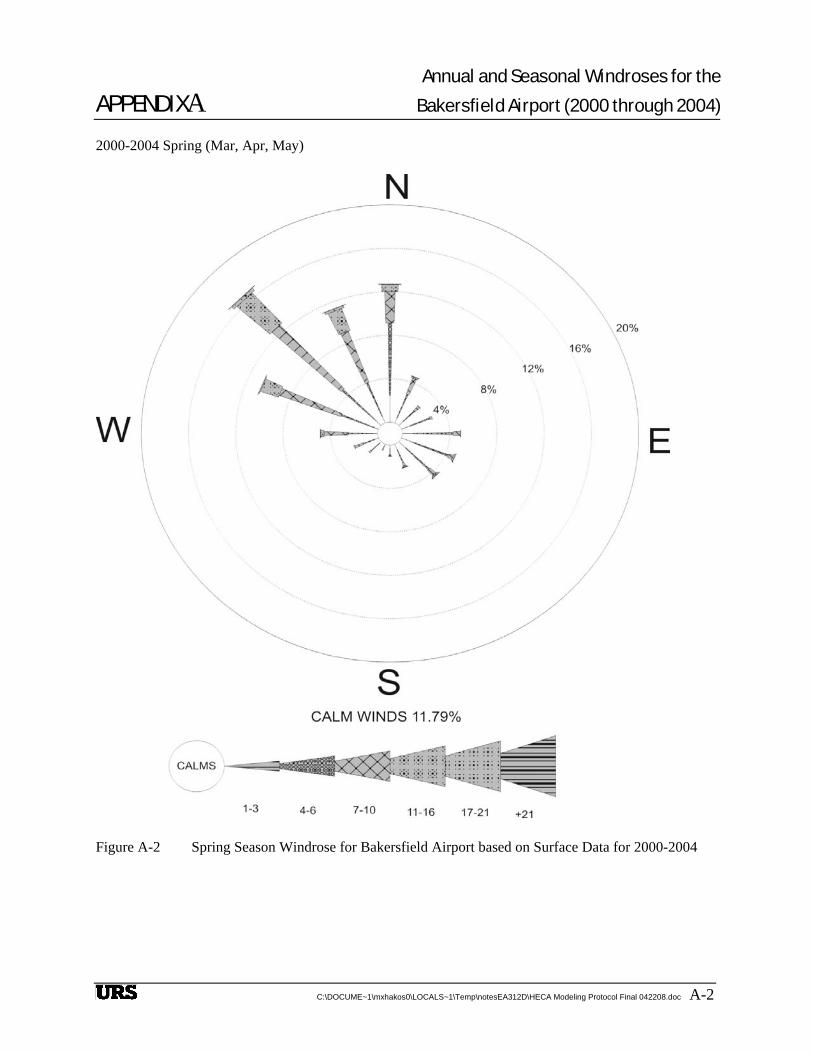
Annual and Seasonal Windroses for the
APPENDIXA Bakersfield Airport (2000 through 2004)
C:\DOCUME~1\mxhakos0\LOCALS~1\Temp\notesEA312D\HECA Modeling Protocol Final 042208.doc A-2
2000-2004 Spring (Mar, Apr, May)
Figure A-2 Spring Season Windrose for Bakersfield Airport based on Surface Data for 2000-2004

Annual and Seasonal Windroses for the
APPENDIXA Bakersfield Airport (2000 through 2004)
C:\DOCUME~1\mxhakos0\LOCALS~1\Temp\notesEA312D\HECA Modeling Protocol Final 042208.doc A-3
2000-2004 Summer (Jun, July, Aug)
Figure A-3 Summer Season Windrose for Bakersfield Airport based on Surface Data for 2000-2004

Annual and Seasonal Windroses for the
APPENDIXA Bakersfield Airport (2000 through 2004)
C:\DOCUME~1\mxhakos0\LOCALS~1\Temp\notesEA312D\HECA Modeling Protocol Final 042208.doc A-4
2000-2004 Fall (Sep, Oct, Nov)
Figure A-4 Fall Season Windrose for Bakersfield Airport based on Surface Data for 2000-2004

Annual and Seasonal Windroses for the
APPENDIXA Bakersfield Airport (2000 through 2004)
C:\DOCUME~1\mxhakos0\LOCALS~1\Temp\notesEA312D\HECA Modeling Protocol Final 042208.doc A-5
2000-2004 (Dec, Jan, Feb)
Figure A-5 Winter Season Windrose for Bakersfield Airport based on Surface Data for 2000-2004


Appendix C-2
Agency Comments on Modeling Protocol
CEC and EPA


CEC Comments on the Modeling Protocol for Hydrogen Energy California Project
Note: Applicant’s Response provided in italic font following comment.
Ozone Limiting
On page 4-3, the modeling protocol states that the applicant will use ozone limiting method (OLM) to estimate NOx impacts. On page 4-8, the modeling protocol states that the applicant will use meteorological data from 2000 through 2004 and on page 4-9, the modeling protocol states that the applicant will use ambient ozone monitoring data from 2004 through 2006. It is not discussed in the protocol how the applicant intends to apply the OLM when using ambient monitoring data from one set of years (2004-2006) to the modeling results generated from a different set of years (2000-2004).
Applicant’s Response – The modeling performed using the Ozone Limiting Method used ozone data from the same years corresponding to the meteorological data. The background monitoring data used to estimate criteria pollutant impacts used the highest reported value from the most recent three years of available data.
Project Description
In general, the modeling protocol demonstrates a reasonable approach, however, due to the number of sources and complexity of the proposed power plant, it is difficult to determine what sources are being modeled and under what operating conditions. For example, the project will have two cooling towers, one for the CTGs and one for the air separator. However, it is not possible for staff to determine which (or if both) towers are represented in Table 4-2 (on page 4-6)…which is simply labeled “Cooling Towers.” Therefore, staff recommends that the applicant prepare a more detailed description of the proposed facility components, their expected emission rates, operation (startup, shutdown normal operation, power augmented, etc), and hours of operation per quarter. Additionally, the use of the LMS100 as a backup power source for the facility needs more explanation, what is the purpose of a 100 MW of backup power?
Applicant’s Response – More detailed explanations of the sources and their operations including startup may be round in Section 2 Project Description, and Section 5.1 Air Quality, and in the Air Quality Appendix C. The Auxiliary Combustion Gas Turbine is to be used to supply additional peaking power both for HECA and for the external market.


EPA Comments on Hydrogen Energy Project, Kern County Note: Applicant’s Response provided in italic font following comment. 3.3 A discussion of a Class II visibility analysis should be included. Applicant’s Response – Please see the Visual Resources Section of the AFC for discussions on the visible plumes formed from the cooling towers and the HRSG turbine. 4.2 Please describe the methodology used to determine the surface characteristics for input to AERMET. The methodology should be consistent with the AERMOD Implementation Guide. 4.6.1 Please provide a more detailed justification for the representativeness of the meteorological data. Applicant’s Combined Response to 4.2 ad 4.6.1 – According to the Guidance for Air Dispersion Modeling - San Joaquin Valley Air Pollution Control District (08/06 Rev 1.2), the District prepared regional meteorological data sets for use in the AERMOD. The data set is available online. The District expressed that "The availability of standard meteorological data will reduce inconsistencies in data quality and requests to the regulatory agency on obtaining data." The District used the following meteorological elements in AERMET processing for the 5 year period from 2000 to 2004: ceiling height, wind speed, wind direction, air temperature, total cloud opacity, and total cloud amount. The surface data station used was Bakersfield and the upper air station used was Oakland, CA. The District assumed that surface conditions are the weighted average over a radius of 3 km from the meteorological station split into 8 sectors and it is described in section 5.4 in the guidance. Appendix E in the Guidance shows a detailed description of the surface characteristics (Albedo, Bowen Ratio and Surface roughness) processed. The analysis used the "Bakersfield" meteorological data set available from the District's webpage: http://www.valleyair.org/busind/pto/Tox_Resources/AirQualityMonitoring.htm. The guidance shows "Bakersfield" data set is most applicable for all of Kern County area. The guidance also describes that "the District meteorological data provides a standard data set that can be used for air quality studies using AERMOD. The regional data sets should not be modified. Therefore, the HECA project used the District’s model-ready AERMET data set. 5. The NPS has requested that “for future PSD applicants, we ask that large sources (large emissions) complete an air quality analyses for Class I areas beyond 100 km and we be given the opportunity to review the modeling protocol and PSD applications for large sources.” Applicant’s Response – Comment Noted.


Appendix C-3
HECA Downwash Structure Information


Dow
nwas
h St
ruct
ures
HE
CA
Bui
ldin
gs
Bui
ldin
g N
ame
Com
men
tN
umbe
r of
Tier
sTi
er
Num
ber
Bas
e E
leva
tion
Tier
H
eigh
tN
umbe
r of
Cor
ners
Cor
ner 1
E
ast (
X)
Cor
ner 1
N
orth
(Y)
(ft)
(ft)
(m)
(m)
1K
O_D
RU
MFl
are
KO
Dru
m1
139
050
1728
3359
.439
0963
32
GA
SIF
IER
Gas
sifie
r Stru
ctur
e1
139
020
04
2831
84.2
3909
621
3S
LRY
PR
EP
Slu
rry
Pre
para
tion
Bui
ldin
g1
139
018
54
2832
5239
0962
44
AS
U_C
OM
PA
SU
Mai
n A
ir C
ompr
esso
r Enc
losu
re1
142
040
428
2485
.239
0937
95
LOX
_TA
NK
Liqu
id O
xyge
n S
epar
atio
n Ta
nk1
142
090
828
2542
.739
0933
26
HR
SG
Hea
t Rec
over
y S
team
Gen
erat
or1
139
090
828
2683
3909
552
7C
TGC
ombu
stio
n Tu
rbin
e G
ener
ator
11
390
5018
2826
82.7
3909
546
8S
TGS
team
Tur
bine
Gen
erat
or S
truct
ure
11
390
5028
2826
3839
0951
39
AG
RA
GR
Ref
riger
atio
n C
ompr
esso
r Enc
losu
re1
139
040
428
3020
.439
0959
810
CO
2C
O2
Com
pres
sor E
nclo
sure
11
390
504
2830
14.4
3909
521
11FI
NE
SLA
GFi
ne S
lag
Han
dlin
g E
nclo
sure
11
390
704
2832
04.4
3909
484
12O
_DE
EP
_1P
ower
Dis
tribu
tion
Cen
ter -
Dee
pwel
l Inj
11
390
254
2827
88.9
3909
363
13O
_DE
EP
_2P
ower
Dis
tribu
tion
Cen
ter -
Dee
pwel
l Inj
11
390
254
2827
95.5
3909
359
14O
_DE
EP
_3P
ower
Dis
tribu
tion
Cen
ter -
Dee
pwel
l Inj
11
390
254
2827
95.3
3909
353
15O
_PB
LK_1
Pow
er D
istri
butio
n C
ente
r - P
ower
Blo
ck1
139
025
428
2694
.639
0951
816
O_P
BLK
_2P
ower
Dis
tribu
tion
Cen
ter -
Pow
er B
lock
11
390
254
2826
88.3
3909
499
17O
_PB
LK_3
Pow
er D
istri
butio
n C
ente
r - P
ower
Blo
ck1
139
025
428
2687
.239
0950
718
O_P
BLK
_4P
ower
Dis
tribu
tion
Cen
ter -
Pow
er B
lock
11
390
254
2827
05.7
3909
513
19O
_PB
LK_5
Pow
er D
istri
butio
n C
ente
r - P
ower
Blo
ck1
139
025
428
2705
.439
0950
420
O_P
BLK
_6P
ower
Dis
tribu
tion
Cen
ter -
Pow
er B
lock
11
390
254
2827
05.2
3909
499
21O
_PB
LK_7
Pow
er D
istri
butio
n C
ente
r - P
ower
Blo
ck1
139
025
428
2705
3909
494
22O
_PB
LK_8
Pow
er D
istri
butio
n C
ente
r - P
ower
Blo
ck1
139
025
428
2704
.939
0948
923
O_A
SU
Pow
er D
istri
butio
n C
ente
r - A
SU
Are
a1
142
025
428
2495
3909
413
24O
_SU
LF_1
Pow
er D
istri
butio
n C
ente
r - S
ulfu
r Loa
di1
139
025
428
2941
.339
0951
525
O_S
ULF
_2P
ower
Dis
tribu
tion
Cen
ter -
Sul
fur L
oadi
11
390
254
2829
35.4
3909
487
26O
_SU
LF_3
Pow
er D
istri
butio
n C
ente
r - S
ulfu
r Loa
di1
139
025
428
2935
.639
0949
227
O_S
ULF
_4P
ower
Dis
tribu
tion
Cen
ter -
Sul
fur L
oadi
11
390
254
2829
35.8
3909
497
28O
_SU
LF_5
Pow
er D
istri
butio
n C
ente
r - S
ulfu
r Loa
di1
139
025
428
2935
.939
0950
129
O_S
ULF
_6P
ower
Dis
tribu
tion
Cen
ter -
Sul
fur L
oadi
11
390
254
2829
34.1
3909
511

30O
_SU
LF_7
Pow
er D
istri
butio
n C
ente
r - S
ulfu
r Loa
di1
139
025
428
2952
.239
0950
331
O_S
ULF
_8P
ower
Dis
tribu
tion
Cen
ter -
Sul
fur L
oadi
11
390
254
2829
50.5
3909
496
32O
_CO
OL_
1P
ower
Dis
tribu
tion
Cen
ter -
Coo
ling
Tow
e1
139
025
428
2977
.239
0942
333
O_C
OO
L_2
Pow
er D
istri
butio
n C
ente
r - C
oolin
g To
we
11
390
254
2829
80.6
3909
416
34O
_CO
OL_
3P
ower
Dis
tribu
tion
Cen
ter -
Coo
ling
Tow
e1
139
025
428
2986
.139
0941
635
O_S
OU
R_1
Pow
er D
istri
butio
n C
ente
r - S
our S
hift
A1
139
025
428
3097
.739
0953
136
O_S
OU
R_2
Pow
er D
istri
butio
n C
ente
r - S
our S
hift
A1
139
025
428
3091
.939
0950
337
O_S
OU
R_3
Pow
er D
istri
butio
n C
ente
r - S
our S
hift
A1
139
025
428
3092
.139
0950
838
O_S
OU
R_4
Pow
er D
istri
butio
n C
ente
r - S
our S
hift
A1
139
025
428
3092
.339
0951
339
O_S
OU
R_5
Pow
er D
istri
butio
n C
ente
r - S
our S
hift
A1
139
025
428
3092
.439
0951
840
O_S
OU
R_6
Pow
er D
istri
butio
n C
ente
r - S
our S
hift
A1
139
025
428
3090
.639
0952
741
O_S
OU
R_7
Pow
er D
istri
butio
n C
ente
r - S
our S
hift
A1
139
025
428
3108
.739
0952
042
O_S
OU
R_8
Pow
er D
istri
butio
n C
ente
r - S
our S
hift
A1
139
025
428
3107
3909
512
43O
_SLA
G_1
Pow
er D
istri
butio
n C
ente
r - F
ine
Sla
g H
a1
139
025
428
3185
.239
0953
644
O_S
LAG
_2P
ower
Dis
tribu
tion
Cen
ter -
Fin
e S
lag
Ha
11
390
254
2831
79.3
3909
508
45O
_SLA
G_3
Pow
er D
istri
butio
n C
ente
r - F
ine
Sla
g H
a1
139
025
428
3179
.539
0951
246
O_S
LAG
_4P
ower
Dis
tribu
tion
Cen
ter -
Fin
e S
lag
Ha
11
390
254
2831
79.6
3909
517
47O
_SLA
G_5
Pow
er D
istri
butio
n C
ente
r - F
ine
Sla
g H
a1
139
025
428
3179
.839
0952
248
O_S
LAG
_6P
ower
Dis
tribu
tion
Cen
ter -
Fin
e S
lag
Ha
11
390
254
2831
7839
0953
249
O_S
LAG
_7P
ower
Dis
tribu
tion
Cen
ter -
Fin
e S
lag
Ha
11
390
254
2831
96.1
3909
524
50O
_SLA
G_8
Pow
er D
istri
butio
n C
ente
r - F
ine
Sla
g H
a1
139
025
428
3194
.439
0951
651
O_S
ILO
_1P
ower
Dis
tribu
tion
Cen
ter -
Fee
dsto
ck S
t1
139
025
428
3647
3909
453
52O
_SIL
O_2
Pow
er D
istri
butio
n C
ente
r - F
eeds
tock
St
11
390
254
2836
53.6
3909
449
53O
_SIL
O_3
Pow
er D
istri
butio
n C
ente
r - F
eeds
tock
St
11
390
254
2836
53.4
3909
443
54O
_PA
RK
_1P
ower
Dis
tribu
tion
Cen
ter -
Par
king
Are
a1
135
025
428
3911
.739
0942
955
O_P
AR
K_2
Pow
er D
istri
butio
n C
ente
r - P
arki
ng A
rea
11
350
254
2839
15.5
3909
434
56O
_PA
RK
_3P
ower
Dis
tribu
tion
Cen
ter -
Par
king
Are
a1
135
025
428
3921
3909
434
57A
SU
_CO
OL
AS
U C
oolin
g To
wer
s1
142
050
828
2468
.139
0927
758
PW
R_C
OO
LP
ower
Blo
ck a
nd G
assi
ficat
ion
Coo
ling
To1
139
050
1228
2836
.539
0940
159
EM
ER
_GN
1E
mer
genc
y G
ener
ator
- 1
11
390
204
2827
20.5
3909
516
60E
ME
R_G
N2
Em
erge
ncy
Gen
erat
or -
21
139
020
428
2720
.139
0950
661
AU
X_B
OIL
Aux
iliar
y B
oile
r1
139
080
428
2762
.139
0962
662
OFF
ICE
SC
ontro
l Roo
m -
Lab
- Adm
in -
Whs
e - M
ain
11
350
354
2838
66.9
3909
394
63A
UX
_CTG
Aux
iliar
y C
TG S
truct
ure
11
390
4520
2826
38.6
3909
621
64O
_WA
TR_1
Pw
r Dis
t. C
ente
r - W
ater
Tre
at. A
rea
- 11
134
025
428
3836
.639
0966
565
O_W
ATR
_2P
wr D
ist.
Cen
ter -
Wat
er T
reat
. Are
a - 2
11
340
254
2838
45.9
3909
669
66O
_WA
TR_3
Pw
r Dis
t. C
ente
r - W
ater
Tre
at. A
rea
- 31
134
025
428
3838
.939
0967
067
CO
NTR
OL
Com
mon
Con
trol -
Adm
in -
Lab
11
350
324
2838
65.1
3909
344

68E
ME
RR
ES
PE
mer
genc
y R
espo
nse
Med
ical
Cen
ter
11
350
224
2838
67.8
3909
419
Tank
s
Tank
Nam
eD
escr
iptio
nB
ase
Ele
vatio
nC
ente
r E
ast (
X)
Cen
ter
Nor
th (Y
)Ta
nk
Hei
ght
Tank
D
iam
eter
(ft)
(m)
(m)
(m)
(m)
1R
AW
WA
TER
Raw
Wat
er T
ank
340
2839
33.9
3909
529
14.6
342
.69
2TR
EA
TD_W
Trea
ted
Wat
er T
ank
340
2839
20.1
3909
582
14.6
330
.48
3FI
RE
WA
TRFi
rew
ater
Sto
rage
Tan
k34
028
3882
.639
0950
212
.19
33.5
44
OU
TFA
L_W
Out
fall
Wat
er T
ank
340
2827
92.9
3909
291
12.1
915
.24
5C
ON
DE
NS
AC
onde
nsat
e S
tora
ge T
ank
390
2827
68.2
3909
543
7.31
4812
.191
416
DE
MIN
ER
AD
emin
erai
zed
Sto
rage
Tan
k39
028
2767
.639
0952
712
.191
412
.191
417
SO
UR
_WTR
Sou
r Wat
er S
tripp
er F
eed
Tank
390
2829
0339
0953
19.
7531
10.9
7226
8M
ETH
NL_
WM
etha
nol S
tora
ge T
ank
- Wes
t39
028
2996
.539
0944
512
.191
412
.191
419
ME
THN
L_E
Met
hano
l Sto
rage
Tan
k - E
ast
390
2830
20.9
3909
444
12.1
914
12.1
9141
10S
ETT
LER
Set
tler
390
2832
32.7
3909
517
10.6
6837
.153
3111
GR
EY
_WTR
Gre
y W
ater
Tan
k39
028
3257
.639
0949
612
.191
418
.287
1112
PR
OC
_WTR
Pro
cess
Wat
er T
reat
men
t Fee
d Ta
nk39
028
3243
3909
481
9.75
3118
.287
1113
SIL
O_N
Feed
stoc
k S
tora
ge S
ilos
- N
orth
390
2836
2139
0950
053
.337
424
.352
3314
SIL
O_C
Feed
stoc
k S
tora
ge S
ilos
- Cen
tral
390
2836
20.1
3909
474
53.3
374
24.3
5233
15S
ILO
_SFe
edst
ock
Sto
rage
Silo
s - S
outh
390
2836
19.2
3909
447
53.3
374
24.3
5233
16S
LUR
TK_N
Slu
rry
Run
Tan
k - N
390
2832
43.3
3909
600
22.8
611
.734
2317
SLU
RTK
_CS
lurr
y R
un T
ank
- C39
028
3242
.839
0958
522
.86
11.7
3423
18S
LUR
TK_S
Slu
rry
Run
Tan
k - S
390
2832
42.2
3909
570
22.8
611
.734
2319
AIR
_SE
PA
ir S
epar
atio
n C
olum
n C
an42
028
2469
.539
0933
662
.48
8.88
20A
GR
_CO
LMA
GR
Met
hano
l Was
h C
olum
n39
028
2998
.939
0963
571
.624
55.
3337
4

Appendix C-4
CALMET/CALPUFF Air Quality Modeling Impact Analysis


CALMET/CALPUFF Air Quality Modeling Impact Analysis for Far-Field Class I Areas FOR THE HYDROGEN ENERGY CALIFORNIA (HECA) PROJECT Kern County, CA Prepared for:
U.S. Environmental Protection Agency Region IX U.S. Forest Service Prepared by:
1333 Broadway, Suite 800 Oakland, CA 94612 July 2008


APPENDIX C4 CALMET/CALPUFF
AIR QUALITY MODELING IMPACT ANALYSIS FOR FAR-FIELD CLASS I AREAS
C4-i
Table of Contents
1.0 Background.................................................................................................................C4-1
1.1 Model Selection and Setup ..........................................................................C4-1 1.2 Domain.........................................................................................................C4-2
2.0 CALMET Processing..................................................................................................C4-5
2.1 MM5 Data....................................................................................................C4-5 2.2 Hourly Surface and Precipitation Data ........................................................C4-5 2.3 Upper Air Data.............................................................................................C4-6 2.4 CALMET ZFACE and ZIMAX Settings.....................................................C4-7 2.5 Wind Field Model Options ..........................................................................C4-7 2.6 LULC and TERREL processing ..................................................................C4-7
3.0 CALPUFF Processing...............................................................................................C4-11
3.1 Receptors of Class I Areas.........................................................................C4-11 3.2 Sources Included in CALPUFF Modeling.................................................C4-11 3.3 CALPUFF Parameters ...............................................................................C4-21 3.4 PSD Class I Increment Significance Analysis ...........................................C4-22 3.5 Class I Area Visibility Reduction Analysis ...............................................C4-22 3.6 Total Nitrogen and Sulfur Deposition Analysis.........................................C4-23
4.0 Modeling Results ......................................................................................................C4-24
4.1 CALPUFF Modeling Results.....................................................................C4-24
5.0 References.................................................................................................................C4-26
List of Figures Figure 1 CALMET/CALPUFF Modeling Domain Figure 2 MM5 and CALMET/CALPUFF Modeling Domain Figure 3 Locations of Surface and Precipitation Data Stations Figure 4 3-D Terrain Elevation Contours Figure 5 Land Use Land Cover
List of Tables Table 1 Class I Areas nearby Project Site Table 2 Maximum Emission Rates of Each Averaging Time Period Table 3 Source Location and Parameters

APPENDIX C4 CALMET/CALPUFF AIR QUALITY MODELING IMPACT ANALYSIS FOR FAR-FIELD CLASS I AREAS
C4-ii
Table 4 3-hour Averaged Emission Inventory for CALPUFF (3-hour SO2) Table 5 24-hour Averaged Emission Inventory for CALPUFF (24-hour NOx, SO2, and
PM10 and Visibility) Table 6 Annual Averaged Emission Inventory for CALPUFF (Annual NOx, SO2, and
PM10 and Deposition) Table 7 Size Distribution of SOA (NPS, 2008) Table 8 PSD Class I Increment Significance Analysis – CALPUFF Results Table 9 Visibility Analysis – CALPUFF Results Table 10 Total Nitrogen and Sulfur Deposition Analysis – CALPUFF Results

APPENDIX C4 CALMET/CALPUFF
AIR QUALITY MODELING IMPACT ANALYSIS FOR FAR-FIELD CLASS I AREAS
C4-1
1.0 BACKGROUND In accordance with comments from the National Park Service (NPS), U.S. Forest Service (USFS) and U.S. Environmental Protection Agency (USEPA) Region 9 regarding far-field air quality modeling analysis for the proposed Hydrogen Energy California (HECA) project, a refined CALPUFF modeling analysis was performed in conjunction with the CALMET diagnostic meteorological model. Based on the written comments from NPS and EPA and verbal comments from FS, the refined CALPUFF modeling considered only San Rafael Wilderness Class I PSD area for the analysis.
1.1 Model Selection and Setup The CALPUFF air dispersion model is the preferred model for long-range transport recommended by the Federal Land Managers’ Air Quality Related Value Workgroup (FLAG) guidance and the Interagency Working Group on Air Quality Modeling (IWAQM) phase 2 summary report. To estimate air quality impacts at distances greater than 50 km, the CALPUFF model was used in conjunction with the CALMET diagnostic meteorological model. CALPUFF is a puff-type model that can incorporate three-dimensionally varying wind fields, wet and dry deposition, and atmospheric gas and particle phase chemistry.
The CALMET model is used to prepare the necessary gridded wind fields for use in the CALPUFF model. CALMET can accept as input; mesoscale meteorological data (MM5 data), surface, upper air, precipitation, cloud cover, and over-water meteorological data (all in a variety of input formats). These data are merged and the effects of terrain and land cover types are estimated. This process results in the generation of gridded 3-D wind field that accounts for the effects of slope flows, terrain blocking effects, flow channelization, and spatially varying land use types.
The development of model inputs and options for CALMET/CALPUFF processor was based on guidance provided in following references:
• Federal Land Managers’ Air Quality Related Values Workgroup (FLAG) Phase I Report (December 2000);
• Interagency Working Group on Air Quality Modeling (IWAQM) Phase 2 Summary Report and Recommendations for Modeling Long Range Transport Impacts (December 1998);
• CALMET/CALPUFF Protocol for BART Exemption Screening Analysis for Class I Areas in the Western United States (August 15, 2006);
• CALPUFF Reviewer’s Guide (DRAFT) prepared for USDA Forest Service and National Park Service (September 2005); and
• Permit application PSD particulate matter speciation methodology developed by Don Shepherd, National Park Service (2008).
Key input and model options selected are discussed in the following sections.
The most recent EPA-approved version of the CALMET, CALPUFF, CALPOST system (version 5.8, version 5.8 and version 5.6394, respectively) was used.

APPENDIX C4 CALMET/CALPUFF AIR QUALITY MODELING IMPACT ANALYSIS FOR FAR-FIELD CLASS I AREAS
C4-2
1.2 Domain The CALMET/CALPUFF modeling domain was specified using the Lambert Conformal Conic (LCC) Projection system in order to capture the earth curvature of the large modeling domain more accurately for this project. The false easting and northing at the projection origin were both set to zero. The latitude and longitude of the projection origin were set to 35.057 N and 119.643 W, respectively. Matching parallels of latitude 1 and 2 were defined as 34.38 N and 35.67 N, respectively. The choice of the matching parallels was made according to the latitudinal extent of the modeling domain, and therefore the parallels should be contained within the modeling domain in order to minimize distortion. An accepted rule-of-thumb is the rule of sixths which calls for one parallel to be placed 1/6th of the domain’s north-south extent south of the domain’s north edge, and an identical distance north of the domain’s south edge (WDEQ, 2006). The modeling domain was defined using a grid-cell arrangement that is 52 cells in X (easting) direction and 54 cells in Y (northing) direction. The grid-cells are 4 kilometers wide. Therefore, the southwest corner of the gird cell (1,1) were set to -101 km and -110 km.
At least 50 km of buffer distance was set between the most outer-boundary of all Class I areas within the modeling domain in order to prevent the loss of mass outside the boundary under some meteorological scenarios that might be associated with transport to nearby Class I areas. The total CALMET/CALPUFF modeling domain is shown in Figure 1. The entire MM5 data set domain is shown for information only in Figure 2.

APPENDIX C4 CALMET/CALPUFF
AIR QUALITY MODELING IMPACT ANALYSIS FOR FAR-FIELD CLASS I AREAS
C4-3
Figure 1 CALMET/CALPUFF Modeling Domain

APPENDIX C4 CALMET/CALPUFF AIR QUALITY MODELING IMPACT ANALYSIS FOR FAR-FIELD CLASS I AREAS
Figure 2 MM5 and CALMET/CALPUFF Modeling Domain
C4-4

APPENDIX C4 CALMET/CALPUFF
AIR QUALITY MODELING IMPACT ANALYSIS FOR FAR-FIELD CLASS I AREAS
C4-5
2.0 CALMET PROCESSING
2.1 MM5 Data A Mesoscale Meteorological Model (MM5) data set was used in conjunction with the actual surface and precipitation meteorological data observations. Three years (2001-2003) of MM5 data were obtained from Western Regional Air Partnership (WRAP). This MM5 data were used for Utah and Nevada’s Best Available Retrofit Technology (BART) analysis by WRAP (WRAP, 2006). The MM5 data had a 36 km resolution. Initial guess wind fields based on hourly 36 km MM5 meteorological fields for 2001, 2002 and 2003 (IPROG =14) was used. MM5 domain is shown in Figure 2.
2.2 Hourly Surface and Precipitation Data CALMET pre-processed hourly surface data were obtained from WRAP’s CALPUFF BART website (WRAP, 2008). WRAP used approximately 190 different surface meteorological data stations for 3-year period (2001 through 2003) for BART analysis. Although thirteen (13) stations are located within the HECA CALPUFF modeling domain, all surface stations were used for this modeling analysis.
This modeling analysis considered the effects of chemical transformations and deposition processes on ambient pollutant concentrations; therefore, observation of precipitation was included in the CALMET analysis. CALMET pre-processed precipitation data was also collected from WRAP’s BART website (WRAP, 2008). The precipitation stations are co-located with surface meteorological data stations. The inverse-distance-squared interpolation scheme was used to generate a gridded precipitation field with hourly precipitation data. The radius of influence for the interpolation method was set to 100 km.
The locations of both surface and precipitation stations used in this analysis are illustrated in Figure 3.

APPENDIX C4 CALMET/CALPUFF AIR QUALITY MODELING IMPACT ANALYSIS FOR FAR-FIELD CLASS I AREAS
Figure 3 Locations of Surface and Precipitation Data Stations
-200 0 200 400 600 800LCC East (km)
-200
0
200
400
600
800
1000
LCC
Nor
th (k
m)
Surface and Precipitation Station
2.3 Upper Air Data No observed upper-air meteorological observations were used as they are redundant to the MM5 data and may introduce spurious artifacts in the wind field (WRAP, 2006). WRAP explains that the twice daily upper-air meteorological observations are used as input with the MM5 model estimates nudged to the observations as part of the Four Dimensional Data Assimilation (FDDA) in the application of the MM5. This results in higher temporal (hourly vs. 12-hour) and spatial (36km vs. ~300 km) resolution upper-air meteorology in the MM5 field that is dynamically
C4-6

APPENDIX C4 CALMET/CALPUFF
AIR QUALITY MODELING IMPACT ANALYSIS FOR FAR-FIELD CLASS I AREAS
C4-7
balanced than contained in the upper-air observations. Therefore, the use of the upper-air observations with CALMET is not needed and in fact will upset the dynamic balance of the meteorological fields potentially producing spurious vertical velocities (WRAP, 2006).
2.4 CALMET ZFACE and ZIMAX Settings Eleven vertical layers were used with vertical cell face (ZFACE) heights at 0, 20, 100, 200, 350, 500, 750, 1000, 2000, 3000, 4000, and 5000 meters. Maximum mixing height (ZIMAX) was set to 4500 meters based on the WRAP modeling analysis. WRAP introduced Colorado Department of Public Health and Environment (CDPHE) analyses of soundings for summer ozone events in the Denver area (CDPHE 2005). The CDPHE analysis suggests mixing heights in the Denver area are often well above the CALMET default value of 3,000 meters during the summer. A 3,000 m AGL maximum mixing height might be appropriate in the eastern U.S., however in the western U.S. in the summer mixing heights may exceed this value. WRAP expected that mixing heights in excess of the 3,000 m AGL CALMET default maximum would occur in the western States (WRAP, 2006).
2.5 Wind Field Model Options In general, CALMET involves two steps in developing the final wind field. First, the prognostic wind field (such as MM5) is introduced into CALMET as the initial guess field. CALMET then adjusts this field by accounting for the kinematic terrain effects, slope flows, blocking effects, and three-dimensional divergence minimization. The wind field resulting from this step is called the Step 1 wind field. Second, CALMET further adjusts the Step 1 wind field by applying an objective analysis procedure with observational data from selected surface, upper air, and precipitation stations. This step generates the final (Step 2) wind field. The “Diagnostic Wind Module” (DWM) option follows this two-step procedure. In this study, the DWM option was chosen in order to reflect the terrain effects in the wind field. Because several mountain ranges occur within the modeling domain, it was expected that terrain effects would be significant.
The MM5 data were used as the initial guess wind field. The extrapolation of the surface wind data aloft (IEXTRP =-4) was used as recommended by USEPA.
Wind speed and wind direction data from observation stations were only allowed to influence the Step 1 wind field at a distance determined by setting the radius-of-influence parameter. The radius of influence for the surface (RMAX1) was set to 100 km as FLM recommended. The distance from a surface observation station at which the observations and Step 1 wind field were weighted was set to 50 km, which is within the FLM’s recommended range of 20-80 km. Radius of influence for terrain features was set to 10 km. All of these radius-of-influence parameters were set based on CALPUFF Reviewer’s Guide (2005).
2.6 LULC and TERREL processing The CALMET and CALPUFF models incorporate assumptions regarding land-use classification, leaf-area index, and surface roughness length to estimate deposition during transport. These parameters were calculated with a 4 km grid spacing for the modeling domain. U.S. Geological Survey (USGS) 1:250,000 scale digital elevation models (DEMs) and Land Use Land Cover (LULC) classification files were obtained and used to develop the geophysical input files

APPENDIX C4 CALMET/CALPUFF AIR QUALITY MODELING IMPACT ANALYSIS FOR FAR-FIELD CLASS I AREAS
C4-8
required by the CALMET model. U.S. Geological Survey (USGS) 1:250,000 scale (1-degree) DEMs data with 90 meters resolution were obtained from the USGS ftp site: http://edcftp.cr.usgs.gov/pub/data/DEM/250/. Using nine (9) 1-degree DEM data files obtained, terrain pre-processor (TERREL) was processed to produce gridded fields of terrain elevation in the formats compatible with the CALMET. The names of 1 degree DEM quadrangles are as follows: Bakersfield-e, Bakersfield-w, Fresno-e, Fresno-w, Los_angeles-e, Log_angeles-w, Montery-e, San_luis_obispo-e, Santa_maria-e. Figure 4 shows the elevation contours calculated within the model domain.
LULC data (*.gz) were obtained from USGS 250K site, http://edcftp.cr.usgs.gov/pub/data/LULC/. Land Use Data Preprocessors, CTGCOMP and CTGPROC were processed to compress six (6) 250K LULC data files obtained. After processing, the data were quality checked to ensure land use was accurately represented. USGS land use data contains 38 land use categories. These were mapped to 14 categories read by CALMET. The names of 250K LULC quadrangles are as follows: Bakersfield, Fresno, Los_Angeles, Montery, San_luis_obispo, and Santa_maria. Figure 5 shows the plot of land use data.
The outputs of TERREL and CTGPROC were combined in the geo-physical preprocessor (MAKEGEO) to prepare the CALMET geo-physical input file. These inputs include land use type, elevation, surface parameters (surface roughness, length, albedo, bowen ratio, soil heat flux parameter, and vegetation leaf area index) and anthropogenic heat flux.

APPENDIX C4 CALMET/CALPUFF
AIR QUALITY MODELING IMPACT ANALYSIS FOR FAR-FIELD CLASS I AREAS
C4-9
Figure 4 3-D Terrain Elevation Contours
-100 -80 -60 -40 -20 0 20 40 60 80 100LCC East (km)
-100
-80
-60
-40
-20
0
20
40
60
80
100
LCC
Nor
th (k
m)
34.5N
35.0N
35.5N
36.0N120.5W 120.0W 119.5W 119.0W 118.5W
-11003005007009001100130015001700190021002300250027002900310033003500370039004500
Terrain (m)
.
.
LCC Origin: 35.06N, 119.64WMatching Parallels: 34.38N, 35.67N
Mar 15, 200100:00 LST(UTC-0800)
-80 -60 -40 -20 0 20 40 60 80 100
-100
-80
-60
-40
-20
0
20
40
60
80
100
Terrain (m)
010020030040050060070080090010001100120013001400150016001700180019002000210022002300
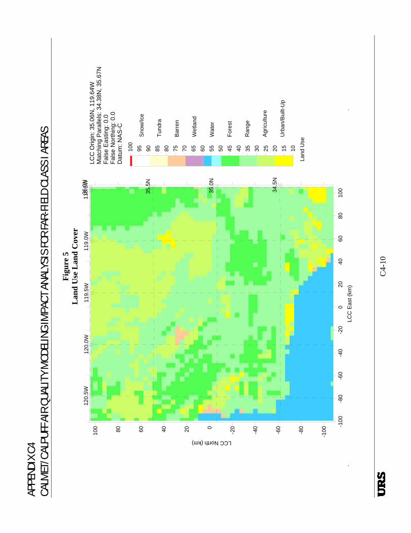
APPE
NDIX
C4
CALM
ET/C
ALPU
FF A
IR Q
UALI
TY M
ODEL
ING
IMPA
CT A
NALY
SIS
FOR
FAR-
FIEL
D CL
ASS
I ARE
AS
Fi
gure
5
Lan
d U
se L
and
Cov
er
-100
-80
-60
-40
-20
020
4060
8010
0LC
C E
ast (
km)
-100-80
-60
-40
-20020406080100
LCC North (km)
34.5
N
35.0
N
35.5
N
36.0
N12
0.5W
120.
0W11
9.5W
119.
0W11
8.5W
Sno
w/Ic
e
Tund
ra
Bar
ren
Wet
land
Wat
er
Fore
st
Ran
ge
Agric
ultu
re
Urb
an/B
uilt-
Up
Land
Use
101520253035404550556065707580859095100
.LC
C O
rigin
: 35.
06N
, 119
.64W
Dat
um: N
AS
-C
Mat
chin
g P
aral
lels
: 34.
38N
, 35.
67N
Fals
e Ea
stin
g: 0
.0Fa
lse
Nor
thin
g: 0
.0
..
C
4-10
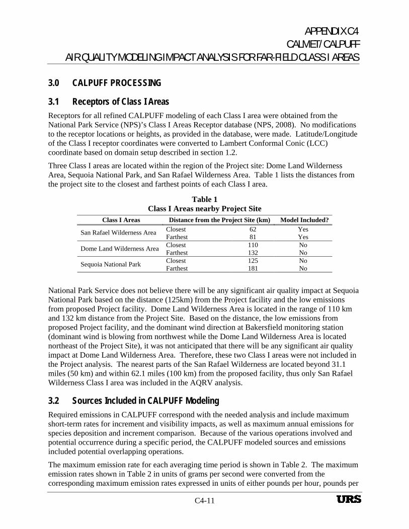
APPENDIX C4 CALMET/CALPUFF
AIR QUALITY MODELING IMPACT ANALYSIS FOR FAR-FIELD CLASS I AREAS
C4-11
3.0 CALPUFF PROCESSING
3.1 Receptors of Class I Areas Receptors for all refined CALPUFF modeling of each Class I area were obtained from the National Park Service (NPS)’s Class I Areas Receptor database (NPS, 2008). No modifications to the receptor locations or heights, as provided in the database, were made. Latitude/Longitude of the Class I receptor coordinates were converted to Lambert Conformal Conic (LCC) coordinate based on domain setup described in section 1.2.
Three Class I areas are located within the region of the Project site: Dome Land Wilderness Area, Sequoia National Park, and San Rafael Wilderness Area. Table 1 lists the distances from the project site to the closest and farthest points of each Class I area.
Table 1 Class I Areas nearby Project Site
Class I Areas Distance from the Project Site (km) Model Included? Closest 62 Yes San Rafael Wilderness Area Farthest 81 Yes Closest 110 No Dome Land Wilderness Area Farthest 132 No Closest 125 No Sequoia National Park Farthest 181 No
National Park Service does not believe there will be any significant air quality impact at Sequoia National Park based on the distance (125km) from the Project facility and the low emissions from proposed Project facility. Dome Land Wilderness Area is located in the range of 110 km and 132 km distance from the Project Site. Based on the distance, the low emissions from proposed Project facility, and the dominant wind direction at Bakersfield monitoring station (dominant wind is blowing from northwest while the Dome Land Wilderness Area is located northeast of the Project Site), it was not anticipated that there will be any significant air quality impact at Dome Land Wilderness Area. Therefore, these two Class I areas were not included in the Project analysis. The nearest parts of the San Rafael Wilderness are located beyond 31.1 miles (50 km) and within 62.1 miles (100 km) from the proposed facility, thus only San Rafael Wilderness Class I area was included in the AQRV analysis.
3.2 Sources Included in CALPUFF Modeling Required emissions in CALPUFF correspond with the needed analysis and include maximum short-term rates for increment and visibility impacts, as well as maximum annual emissions for species deposition and increment comparison. Because of the various operations involved and potential occurrence during a specific period, the CALPUFF modeled sources and emissions included potential overlapping operations.
The maximum emission rate for each averaging time period is shown in Table 2. The maximum emission rates shown in Table 2 in units of grams per second were converted from the corresponding maximum emission rates expressed in units of either pounds per hour, pounds per

APPENDIX C4 CALMET/CALPUFF AIR QUALITY MODELING IMPACT ANALYSIS FOR FAR-FIELD CLASS I AREAS
C4-12
day or tons per year contained in the emissions inventory. The stack parameters of all sources are shown in Table 3.
The CALPUFF modeling included speciation of emissions according to the National Park Service (NPS)’s Particulate Matter Speciation (PMS) method for natural gas combustion turbines. Applying the PMS methodology, 67% of total SO2 was speciated into SO2 and 33% of total SO2 was speciated into SO4. Also, the total PM10 emission from HRSG/Turbine was speciated into Elemental Carbon (EC) and Secondary Organic Aerosol (SOA). The SOA was speciated again into PM0.05, PM0.01, PM0.15, PM0.20, PM0.25, and PM1.0 (indicated as PM0005, PM0010, PM0015, PM0020, PM0025, and PM0100 in the modeling, respectively). The PM10 emissions from other sources were modeled directly as PM10. Direct emissions of the remaining species, HNO3 and NO3, were assumed to be zero for the natural gas burning sources of the project. The modeled emissions are shown in Table 4 (3-hour averaged), Table 5 (24-hour averaged), and Table 6 (annual averaged). The SOA size distribution is shown in Table 7. In addition, total PM emission was separately modeled as INCPM without speciation for incremental PM analysis.
The 3-hour averaged emission rate was used for the 3-hour SO2 impact analysis. The 24-hour averaged emission rate was used for the 24-hour SO2 and 24-hour PM10 impact analyses, and visibility impairment impact analysis. The annual emission rate was used for the annual NOx, annual SO2, and annual PM10 impact analyses as well as nitrogen and sulfur deposition analyses.

APPENDIX C4 CALMET/CALPUFF
AIR QUALITY MODELING IMPACT ANALYSIS FOR FAR-FIELD CLASS I AREAS
C4-13
Table 2 Maximum Emission Rates of Each Averaging Time Period
3-hr (g/s) 24-hr (g/s) Annual (g/s) Source
SO2 NOx SO2 PM10 NOx SO2 PM10 ASUCOOL1 - - - 0.0285 - - 0.0271 ASUCOOL2 - - - 0.0285 - - 0.0271 ASUCOOL3 - - - 0.0285 - - 0.0271 ASUCOOL4 - - - 0.0285 - - 0.0271 PWCOOL1 - - - 0.0382 - - 0.0363 PWCOOL2 - - - 0.0382 - - 0.0363 PWCOOL3 - - - 0.0382 - - 0.0363 PWCOOL4 - - - 0.0382 - - 0.0363 PWCOOL5 - - - 0.0382 - - 0.0363 PWCOOL6 - - - 0.0382 - - 0.0363 PWCOOL7 - - - 0.0382 - - 0.0363 PWCOOL8 - - - 0.0382 - - 0.0363 PWCOOL9 - - - 0.0382 - - 0.0363 PWCOOL10 - - - 0.0382 - - 0.0363 PWCOOL11 - - - 0.0382 - - 0.0363 PWCOOL12 - - - 0.0382 - - 0.0363 PWCOOL13 - - - 0.0382 - - 0.0363 GASCOOL1 - - - 0.0300 - - 0.0285 GASCOOL2 - - - 0.0300 - - 0.0285 GASCOOL3 - - - 0.0300 - - 0.0285 GASCOOL4 - - - 0.0300 - - 0.0285
EMERGEN1 a 0.0024 - - - 0.0022 0.00002 0.0001 EMERGEN2 a - - - - - - -
HRSGSTK 0.8600 3.7618 0.1929 2.3939 4.8092 0.8131 2.8695 FIREPUMP b 0.0005 - - - 0.0026 0.000008 0.000026 AUX_BOIL c - - - - 0.0492 0.0091 0.0224
TAIL_TO 0.2546 0.3276 0.2546 0.0202 0.1694 0.2521 0.0104 CO2_VENT - - - - - - - EL_FLARE 2.1933 0.0720 0.2742 0.0018 0.0049 0.0016 0.0001 GD_FLARE 0.0001 6.6150 0.0001 0.0002 0.1239 0.0001 0.0002
GASVENTA d - - - - - - - GASVENTB 0.0454 0.2948 0.0454 0.0181 0.0606 0.0093 0.0037
GASVENTC d - - - - - - - AUX_CTG e 0.2343 - - - 0.5011 0.1100 0.5912
DC1 - - - 0.0511 - - 0.0109 DC2 - - - 0.0759 - - 0.0163 DC3 - - - 0.0759 - - 0.0163 DC4 - - - 0.0012 - - 0.0010 DC5 - - - 0.0141 - - 0.0112 DC6 - - - 0.0126 - - 0.0099 DC7 - - - 0.0105 - - 0.0083 DC8 - - - 0.0129 - - 0.0102 DC9 - - - 0.0003 - - 0.0003
Notes: a. Assumed that emergency generators will not run on worst case day. b. Assumed that firewater pump will not run on worst case day. c. Auxiliary boiler is not fired at the same time that the HRSG is operating.

APPECALMET/CALPUFF AIR QUALITY MODELING IMP
NDIX C4
ACT ANALYSIS FOR FAR-FIELD CLASS I AREAS
C4-14
d. There are three gasifiers. Only one gasifier warming will be operated at any one time. The emission is from GASVENTB, which results worst impact among three gasifiers.
e. Assumed that auxiliary turbine will not run on worst case day. f. Average sulfur content of the natural gas combusted in the HRSG is assumed. (g/s) = grams per second NOx = oxides of nitrogen PM10 = particulate matter 10 microns in diameter SO2 = sulfur dioxide

APPE
NDIX
C4
CALM
ET/C
ALPU
FF
AIR
QUAL
ITY
MOD
ELIN
G IM
PACT
ANA
LYSI
S FO
R FA
R-FI
ELD
CLAS
S I A
REAS
C4-
15
Tab
le 3
So
urce
Loc
atio
n an
d Pa
ram
eter
s U
TM
E
astin
g U
TM
N
orth
ing
LC
C
X
LC
C
Y
Bas
e E
leva
tion
Stac
k H
eigh
t St
ack
Tem
pera
ture
St
ack
Vel
ocity
St
ack
Dia
met
er
Sour
ce ID
So
urce
Des
crip
tion
(m)
(m)
(km
) (k
m)
(m)
(m)
(K)
(m/s
) (m
) A
SUC
OO
L1
ASU
Coo
ling
Tow
er
2824
76
3909
286
22.7
903
27.5
323
128.
0 17
.24
299.
9 7.
98
9.14
A
SUC
OO
L2
ASU
Coo
ling
Tow
er
2824
91
3909
286
22.8
055
27.5
322
128.
0 17
.24
299.
9 7.
98
9.14
A
SUC
OO
L3
ASU
Coo
ling
Tow
er
2825
06
3909
285
22.8
207
27.5
320
128.
0 17
.24
299.
9 7.
98
9.14
A
SUC
OO
L4
ASU
Coo
ling
Tow
er
2825
21
3909
285
22.8
360
27.5
319
128.
0 17
.24
299.
9 7.
98
9.14
PW
CO
OL1
Po
wer
Blo
ck C
oolin
g To
wer
28
2844
39
0939
2 23
.155
3 27
.647
7 11
8.9
17.2
4 29
9.9
7.98
9.
14
PWC
OO
L2
Pow
er B
lock
Coo
ling
Tow
er
2828
59
3909
391
23.1
706
27.6
476
118.
9 17
.24
299.
9 7.
98
9.14
PW
CO
OL3
Po
wer
Blo
ck C
oolin
g To
wer
28
2874
39
0939
1 23
.185
8 27
.647
5 11
8.9
17.2
4 29
9.9
7.98
9.
14
PWC
OO
L4
Pow
er B
lock
Coo
ling
Tow
er
2828
90
3909
390
23.2
010
27.6
473
118.
9 17
.24
299.
9 7.
98
9.14
PW
CO
OL5
Po
wer
Blo
ck C
oolin
g To
wer
28
2905
39
0939
0 23
.216
3 27
.647
2 11
8.9
17.2
4 29
9.9
7.98
9.
14
PWC
OO
L6
Pow
er B
lock
Coo
ling
Tow
er
2829
20
3909
389
23.2
315
27.6
471
118.
9 17
.24
299.
9 7.
98
9.14
PW
CO
OL7
Po
wer
Blo
ck C
oolin
g To
wer
28
2935
39
0938
9 23
.246
8 27
.646
9 11
8.9
17.2
4 29
9.9
7.98
9.
14
PWC
OO
L8
Pow
er B
lock
Coo
ling
Tow
er
2829
51
3909
388
23.2
620
27.6
468
118.
9 17
.24
299.
9 7.
98
9.14
PW
CO
OL9
Po
wer
Blo
ck C
oolin
g To
wer
28
2966
39
0938
8 23
.277
2 27
.646
7 11
8.9
17.2
4 29
9.9
7.98
9.
14
PWC
OO
L10
Pow
er B
lock
Coo
ling
Tow
er
2829
81
3909
387
23.2
925
27.6
465
118.
9 17
.24
299.
9 7.
98
9.14
PW
CO
OL1
1 Po
wer
Blo
ck C
oolin
g To
wer
28
2996
39
0938
6 23
.307
7 27
.646
4 11
8.9
17.2
4 29
9.9
7.98
9.
14
PWC
OO
L12
Pow
er B
lock
Coo
ling
Tow
er
2830
11
3909
386
23.3
230
27.6
462
118.
9 17
.24
299.
9 7.
98
9.14
PW
CO
OL1
3 Po
wer
Blo
ck C
oolin
g To
wer
28
3027
39
0938
5 23
.338
2 27
.646
1 11
8.9
17.2
4 29
9.9
7.98
9.
14
GA
SCO
OL1
G
asifi
catio
n C
oolin
g To
wer
28
3042
39
0938
5 23
.353
4 27
.646
0 11
8.9
17.2
4 29
9.9
7.98
9.
14
GA
SCO
OL2
G
asifi
catio
n C
oolin
g To
wer
28
3057
39
0938
4 23
.368
7 27
.645
8 11
8.9
17.2
4 29
9.9
7.98
9.
14
GA
SCO
OL3
G
asifi
catio
n C
oolin
g To
wer
28
3072
39
0938
4 23
.383
9 27
.645
7 11
8.9
17.2
4 29
9.9
7.98
9.
14
GA
SCO
OL4
G
asifi
catio
n C
oolin
g To
wer
28
3088
39
0938
3 23
.399
2 27
.645
6 11
8.9
17.2
4 29
9.9
7.98
9.
14
EMER
GEN
1 Em
erge
ncy
Gen
erat
or1
2827
35
3909
508
23.0
438
27.7
611
121.
9 6.
10
677.
6 67
.38
0.37
EM
ERG
EN2
Emer
genc
y G
ener
ator
2 28
2735
39
0950
8 23
.043
8 27
.761
1 12
1.9
6.10
67
7.6
67.3
8 0.
37
HR
SGST
K
HR
SG S
tack
28
2728
39
0954
8 23
.035
0 27
.800
5 11
8.9
65.0
0 34
4.3
11.5
5 6.
10
FIR
EPU
MP
Fire
Wat
er P
ump
Die
sel
Engi
ne
2838
77
3909
536
24.1
842
27.8
194
103.
6 6.
10
727.
6 47
.52
0.21
A
UX
_BO
IL
Aux
iliar
y B
oile
r 28
2803
39
0961
3 23
.108
4 27
.867
3 11
8.9
24.3
8 42
2.0
9.20
1.
37
TAIL
_TO
Ta
il G
as T
herm
al O
xidi
zer
2828
97
3909
483
23.2
056
27.7
401
118.
9 50
.29
922.
0 7.
45
0.76
C
O2_
VEN
T C
O2 V
ent
2834
57
3909
546
23.7
640
27.8
181
118.
9 87
.78
291.
5 55
.92
1.07

APPE
NDIX
C4
CALM
ET/C
ALPU
FF
AIR
QUAL
ITY
MOD
ELIN
G IM
PACT
ANA
LYSI
S FO
R FA
R-FI
ELD
CLAS
S I A
REAS
C
4-16
Tab
le 3
So
urce
Loc
atio
n an
d Pa
ram
eter
s (C
ontin
ued)
U
TM
E
astin
g U
TM
N
orth
ing
LC
C
X
LC
C
Y
Bas
e E
leva
tion
Stac
k H
eigh
t St
ack
Tem
pera
ture
St
ack
Vel
ocity
St
ack
Dia
met
er
Sour
ce ID
So
urce
Des
crip
tion
(m)
(m)
(km
) (k
m)
(m)
(m)
(K)
(m/s
) (m
) EL
_FLA
RE
Elev
ated
Fla
re
2828
81
3909
512
23.1
896
27.7
689
118.
9 65
.00
1273
.0
20.0
0 1.
05
GD
_FLA
RE
Gro
und
Flar
e 28
3357
39
0955
2 23
.663
4 27
.821
8 11
8.9
24.3
8 11
44.3
9.
93
15.2
4 G
ASV
ENTA
G
asifi
er W
arm
ing
Ven
t A
2832
05
3909
611
23.5
106
27.8
762
118.
9 64
.01
338.
7 26
.39
0.30
G
ASV
ENTB
G
asifi
er W
arm
ing
Ven
t B
2832
04
3909
586
23.5
104
27.8
518
118.
9 64
.01
338.
7 26
.39
0.30
G
ASV
ENTC
G
asifi
er W
arm
ing
Ven
t C
2832
03
3909
562
23.5
102
27.8
274
118.
9 64
.01
338.
7 26
.39
0.30
A
UX
_CTG
A
uxili
aryC
ombu
stio
nGas
Turb
ine
2826
24
3909
632
22.9
293
27.8
821
118.
9 33
.53
677.
6 15
.31
4.88
D
C1
Feed
Stoc
k-D
ustC
olle
ctio
n 28
3267
39
0924
0 23
.582
7 27
.507
3 12
1.5
15.0
0 29
1.9
20.9
7 0.
76
DC
2 Fe
edSt
ock-
Dus
tCol
lect
ion
2836
28
3909
468
23.9
371
27.7
448
108.
8 60
.35
291.
9 21
.66
0.91
D
C3
Feed
Stoc
k-D
ustC
olle
ctio
n 28
3613
39
0947
9 23
.921
3 27
.755
7 10
8.8
60.3
5 29
1.9
21.6
6 0.
91
DC
4 Fe
edSt
ock-
Dus
tCol
lect
ion
2836
33
3909
515
23.9
405
27.7
917
108.
8 7.
01
291.
9 22
.70
0.23
D
C5
Feed
Stoc
k-D
ustC
olle
ctio
n 28
3635
39
0960
7 23
.940
4 27
.883
6 10
7.0
24.0
8 29
1.9
12.5
8 0.
66
DC
6 Fe
edSt
ock-
Dus
tCol
lect
ion
2836
14
3909
614
23.9
192
27.8
903
107.
0 24
.08
291.
9 21
.82
0.61
D
C7
Feed
Stoc
k-D
ustC
olle
ctio
n 28
3278
39
0960
9 23
.583
3 27
.876
5 11
8.9
59.4
4 29
1.9
21.5
6 0.
56
DC
8 Fe
edSt
ock-
Dus
tCol
lect
ion
2832
81
3909
588
23.5
869
27.8
556
118.
9 42
.37
291.
9 8.
00
0.56
D
C9
Feed
Stoc
k-D
ustC
olle
ctio
n 28
3279
39
0960
1 23
.584
5 27
.867
9 11
8.9
59.4
4 29
1.9
22.6
0 0.
41
Not
es:
Ass
umed
that
the
tem
pera
ture
of c
oolin
g to
wer
and
dus
t col
lect
ion
is th
e an
nual
ave
rage
d va
lue
from
the
AER
MET
met
eoro
logi
cal d
ata
at B
aker
sfie
ld m
onito
ring
stat
ion.
b.
K
= K
elvi
n km
=
kilo
met
er
LCC
=
Lam
bert
Con
form
al C
onic
m
=
met
er
UTM
=
Uni
vers
al T
rans
vers
e M
erca
tor

APPE
NDIX
C4
CALM
ET/C
ALPU
FF
AIR
QUAL
ITY
MOD
ELIN
G IM
PACT
ANA
LYSI
S FO
R FA
R-FI
ELD
CLAS
S I A
REAS
C4-
17
Tab
le 4
3-
hour
Ave
rage
d E
mis
sion
Inve
ntor
y fo
r C
AL
PUFF
(3-h
our
SO2)
SO
A
Sour
ces
(g/s
) SO
2 SO
4 N
Ox
HN
O3
NO
3 IN
CPM
PM
10
PM00
05
PM00
10
PM00
15
PM00
20
PM00
25
PM01
00
EC
EM
ERG
EN1
2.35
E-03
-
- -
- -
- -
- -
- -
- -
HR
SGST
K
5.73
E-01
4.
30E-
01
2.10
E+01
-
- 2.
39E+
00
- 2.
05E-
01
3.41
E-01
3.
14E-
01
2.05
E-01
1.
50E-
01
1.50
E-01
5.
98E-
01
FIR
EPU
MP
4.70
E-04
-
2.32
E-01
-
- -
- -
- -
- -
- -
TAIL
_TO
2.
55E-
01
- 3.
28E-
01
- -
2.02
E-02
2.
02E-
02
- -
- -
- -
- EL
_FLA
RE
2.19
E+00
-
5.44
E-01
-
- 1.
80E-
03
1.80
E-03
-
- -
- -
- -
GD
_FLA
RE
1.29
E-04
-
7.94
E+00
-
- 1.
58E-
04
1.58
E-04
-
- -
- -
- -
GA
SVEN
TB
4.54
E-02
-
2.95
E-01
-
- 1.
81E-
02
1.81
E-02
-
- -
- -
- -
AU
X_C
TG
1.56
E-01
1.
17E-
01
2.60
E+00
-
- -
- -
- -
- -
- -
Not
es:
(g/s
) =
gram
s per
seco
nd
EC
= El
emen
tal C
arbo
n H
NO
3 =
nitri
c ac
id
INC
PM =
to
tal p
artic
ulat
e m
atte
r em
issi
on
NO
x =
oxid
es o
f nitr
ogen
N
O3
= ni
trate
PM
0005
– P
M01
00 =
par
ticul
ate
mat
ter 5
to 1
00 m
icro
ns in
dia
met
er
PM10
=
parti
cula
te m
atte
r 10
mic
rons
in d
iam
eter
SO
2 =
sulfu
r dio
xide
SO
4 =
sulfa
te c
ompo
und
SOA
=
Seco
ndar
y O
rgan
ic A
eros
ol

APPE
NDIX
C4
CALM
ET/C
ALPU
FF
AIR
QUAL
ITY
MOD
ELIN
G IM
PACT
ANA
LYSI
S FO
R FA
R-FI
ELD
CLAS
S I A
REAS
C
4-18
Tab
le 5
24
-hou
r A
vera
ged
Em
issi
on In
vent
ory
for
CA
LPU
FF (2
4-ho
ur N
Ox,
SO2,
and
PM10
and
Vis
ibili
ty)
SOA
So
urce
s (g
/s)
SO2
SO4
NO
x H
NO
3 N
O3
INC
PM
PM10
PM
0005
PM
0010
PM
0015
PM
0020
PM
0025
PM
0100
E
C
ASU
CO
OL1
-
- -
- -
2.85
E-02
2.
85E-
02
- -
- -
- -
- A
SUC
OO
L2
- -
- -
- 2.
85E-
02
2.85
E-02
-
- -
- -
- -
ASU
CO
OL3
-
- -
- -
2.85
E-02
2.
85E-
02
- -
- -
- -
- A
SUC
OO
L4
- -
- -
- 2.
85E-
02
2.85
E-02
-
- -
- -
- -
PWC
OO
L1
- -
- -
- 3.
82E-
02
3.82
E-02
-
- -
- -
- -
PWC
OO
L2
- -
- -
- 3.
82E-
02
3.82
E-02
-
- -
- -
- -
PWC
OO
L3
- -
- -
- 3.
82E-
02
3.82
E-02
-
- -
- -
- -
PWC
OO
L4
- -
- -
- 3.
82E-
02
3.82
E-02
-
- -
- -
- -
PWC
OO
L5
- -
- -
- 3.
82E-
02
3.82
E-02
-
- -
- -
- -
PWC
OO
L6
- -
- -
- 3.
82E-
02
3.82
E-02
-
- -
- -
- -
PWC
OO
L7
- -
- -
- 3.
82E-
02
3.82
E-02
-
- -
- -
- -
PWC
OO
L8
- -
- -
- 3.
82E-
02
3.82
E-02
-
- -
- -
- -
PWC
OO
L9
- -
- -
- 3.
82E-
02
3.82
E-02
-
- -
- -
- -
PWC
OO
L10
- -
- -
- 3.
82E-
02
3.82
E-02
-
- -
- -
- -
PWC
OO
L11
- -
- -
- 3.
82E-
02
3.82
E-02
-
- -
- -
- -
PWC
OO
L12
- -
- -
- 3.
82E-
02
3.82
E-02
-
- -
- -
- -
PWC
OO
L13
- -
- -
- 3.
82E-
02
3.82
E-02
-
- -
- -
- -
GA
SCO
OL1
-
- -
- -
3.00
E-02
3.
00E-
02
- -
- -
- -
- G
ASC
OO
L2
- -
- -
- 3.
00E-
02
3.00
E-02
-
- -
- -
- -
GA
SCO
OL3
-
- -
- -
3.00
E-02
3.
00E-
02
- -
- -
- -
- G
ASC
OO
L4
- -
- -
- 3.
00E-
02
3.00
E-02
-
- -
- -
- -
HR
SGST
K
1.29
E-01
9.
65E-
02
3.76
E+00
-
- 2.
39E+
00
- -
4.25
E-01
3.
91E-
01
2.55
E-01
1.
87E-
01
1.87
E-01
5.
98E-
01
TAIL
_TO
2.
55E-
01
- 3.
28E-
01
- -
2.02
E-02
2.
02E-
02
- -
- -
- -
- EL
_FLA
RE
2.74
E-01
-
7.20
E-02
-
- 1.
80E-
03
1.80
E-03
-
- -
- -
- -
GD
_FLA
RE
1.07
E-04
-
6.62
E+00
-
- 1.
58E-
04
1.58
E-04
-
- -
- -
- -
GA
SVEN
TB
4.54
E-02
-
2.95
E-01
-
- 1.
81E-
02
1.81
E-02
-
- -
- -
- -
DC
1 -
- -
- -
5.11
E-02
5.
11E-
02
- -
- -
- -
- D
C2
- -
- -
- 7.
59E-
02
7.59
E-02
-
- -
- -
- -
DC
3 -
- -
- -
7.59
E-02
7.
59E-
02
- -
- -
- -
- D
C4
- -
- -
- 1.
23E-
03
1.23
E-03
-
- -
- -
- -
DC
5 -
- -
- -
1.41
E-02
1.
41E-
02
- -
- -
- -
- D
C6
- -
- -
- 1.
26E-
02
1.26
E-02
-
- -
- -
- -
DC
7 -
- -
- -
1.05
E-02
1.
05E-
02
- -
- -
- -
- D
C8
- -
- -
- 1.
29E-
02
1.29
E-02
-
- -
- -
- -
DC
9 -
- -
- -
3.02
E-04
3.
02E-
04
- -
- -
- -
- N
otes
: (g
/s)
= gr
ams p
er se
cond
EC
=
Elem
enta
l Car
bon
HN
O3
= ni
tric
acid
IN
CO
M =
to
tal p
artic
ulat
e m
atte
r em
issi
on
N
Ox
= ox
ides
of n
itrog
en
NO
3 =
nitra
te
PM00
05 –
PM
0100
= p
artic
ulat
e m
atte
r 5 to
100
mic
rons
in d
iam
eter
SO
2 =
sulfu
r dio
xide
SO
4 =
sulfa
te c
ompo
und
SOA
=
Seco
ndar
y O
rgan
ic A
eros
ol

APPE
NDIX
C4
CALM
ET/C
ALPU
FF
AIR
QUAL
ITY
MOD
ELIN
G IM
PACT
ANA
LYSI
S FO
R FA
R-FI
ELD
CLAS
S I A
REAS
C4-
19
Tab
le 6
A
nnua
l Ave
rage
d E
mis
sion
Inve
ntor
y fo
r C
AL
PUFF
(Ann
ual N
Ox,
SO2,
and
PM10
and
Dep
ositi
on) SO
A
Sour
ces
(g/s
) SO
2 SO
4 N
Ox
HN
O3
NO
3 IN
CPM
PM
10
PM00
05
PM00
10
PM00
15
PM00
20
PM00
25
PM01
00
EC
A
SUC
OO
L1
- -
- -
- 2.
71E-
02
2.71
E-02
-
- -
- -
- -
ASU
CO
OL2
-
- -
- -
2.71
E-02
2.
71E-
02
- -
- -
- -
- A
SUC
OO
L3
- -
- -
- 2.
71E-
02
2.71
E-02
-
- -
- -
- -
ASU
CO
OL4
-
- -
- -
2.71
E-02
2.
71E-
02
- -
- -
- -
- PW
CO
OL1
-
- -
- -
3.63
E-02
3.
63E-
02
- -
- -
- -
- PW
CO
OL2
-
- -
- -
3.63
E-02
3.
63E-
02
- -
- -
- -
- PW
CO
OL3
-
- -
- -
3.63
E-02
3.
63E-
02
- -
- -
- -
- PW
CO
OL4
-
- -
- -
3.63
E-02
3.
63E-
02
- -
- -
- -
- PW
CO
OL5
-
- -
- -
3.63
E-02
3.
63E-
02
- -
- -
- -
- PW
CO
OL6
-
- -
- -
3.63
E-02
3.
63E-
02
- -
- -
- -
- PW
CO
OL7
-
- -
- -
3.63
E-02
3.
63E-
02
- -
- -
- -
- PW
CO
OL8
-
- -
- -
3.63
E-02
3.
63E-
02
- -
- -
- -
- PW
CO
OL9
-
- -
- -
3.63
E-02
3.
63E-
02
- -
- -
- -
- PW
CO
OL1
0 -
- -
- -
3.63
E-02
3.
63E-
02
- -
- -
- -
- PW
CO
OL1
1 -
- -
- -
3.63
E-02
3.
63E-
02
- -
- -
- -
- PW
CO
OL1
2 -
- -
- -
3.63
E-02
3.
63E-
02
- -
- -
- -
- PW
CO
OL1
3 -
- -
- -
3.63
E-02
3.
63E-
02
- -
- -
- -
- G
ASC
OO
L1
- -
- -
- 2.
85E-
02
2.85
E-02
-
- -
- -
- -
GA
SCO
OL2
-
- -
- -
2.85
E-02
2.
85E-
02
- -
- -
- -
- G
ASC
OO
L3
- -
- -
- 2.
85E-
02
2.85
E-02
-
- -
- -
- -
GA
SCO
OL4
-
- -
- -
2.85
E-02
2.
85E-
02
- -
- -
- -
- EM
ERG
EN1
2.01
E-05
-
2.22
E-03
-
- 1.
15E-
04
1.15
E-04
-
- -
- -
- -
HR
SGST
K
5.42
E-01
4.
07E-
01
4.81
E+00
-
- 2.
87E+
00
- 2.
62E-
01
4.36
E-01
4.
01E-
01
2.62
E-01
1.
92E-
01
1.92
E-01
7.
17E-
01
FIR
EPU
MP
8.05
E-06
-
2.64
E-03
-
- 2.
64E-
05
2.64
E-05
-
- -
- -
- -
AU
X_B
OIL
9.
13E-
03
- 4.
92E-
02
- -
2.24
E-02
2.
24E-
02
- -
- -
- -
- TA
IL_T
O
2.52
E-01
-
1.69
E-01
-
- 1.
04E-
02
1.04
E-02
-
- -
- -
- -
EL_F
LAR
E 1.
58E-
03
- 4.
91E-
03
- -
1.23
E-04
1.
23E-
04
- -
- -
- -
- G
D_F
LAR
E 1.
29E-
04
- 1.
24E-
01
- -
1.89
E-04
1.
89E-
04
- -
- -
- -
- G
ASV
ENTB
9.
32E-
03
- 6.
06E-
02
- -
3.73
E-03
3.
73E-
03
- -
- -
- -
- A
UX
_CTG
7.
33E-
02
5.50
E-02
5.
01E-
01
- -
5.91
E-01
-
5.83
E-02
9.
71E-
02
8.93
E-02
5.
83E-
02
4.27
E-02
4.
27E-
02
1.48
E-01
D
C1
- -
- -
- 1.
09E-
02
1.09
E-02
-
- -
- -
- -
DC
2 -
- -
- -
1.63
E-02
1.
63E-
02
- -
- -
- -
- D
C3
- -
- -
- 1.
63E-
02
1.63
E-02
-
- -
- -
- -
DC
4 -
- -
- -
9.69
E-04
9.
69E-
04
- -
- -
- -
- D
C5
- -
- -
- 1.
12E-
02
1.12
E-02
-
- -
- -
- -
DC
6 -
- -
- -
9.94
E-03
9.
94E-
03
- -
- -
- -
- D
C7
- -
- -
- 8.
25E-
03
8.25
E-03
-
- -
- -
- -
DC
8 -
- -
- -
1.02
E-02
1.
02E-
02
- -
- -
- -
- D
C9
- -
- -
- 3.
02E-
04
3.02
E-04
-
- -
- -
- -
Not
es:
(g/s
) =
gram
s per
seco
nd
EC
= El
emen
tal C
arbo
n H
NO
3 =
nitr
ic a
cid
INC
OM
= t
otal
par
ticul
ate
mat
ter e
mis
sion
N
Ox
= ox
ides
of n
itrog
en
NO
3 =
nitra
te
PM00
05 –
PM
0100
= p
artic
ulat
e m
atte
r 5 to
100
mic
rons
in d
iam
eter
PM10
=
parti
cula
te m
atte
r 10
mic
rons
in d
iam
eter
SO
2 =
sulfu
r dio
xide
SO
4 =
sulfa
te c
ompo
und
SOA
=
Seco
ndar
y O
rgan
ic A
eros
ol

APPE
NDIX
C4
CALM
ET/C
ALPU
FF
AIR
QUAL
ITY
MOD
ELIN
G IM
PACT
ANA
LYSI
S FO
R FA
R-FI
ELD
CLAS
S I A
REAS
C
4-20
Th
is P
age
Inte
ntio
nally
Lef
t Bla
nk

APPENDIX C4 CALMET/CALPUFF
AIR QUALITY MODELING IMPACT ANALYSIS FOR FAR-FIELD CLASS I AREAS
C4-21
Table 7 Size Distribution of SOA (NPS, 2008)
Species Name Size Distribution (%)
Geometric Mass Mean Diameter
(microns)
Geometric Std. Deviation (microns)
SO4 100 0.48 0.50 NO3 100 0.48 0.50
PM0005 15 0.05 0.00 PM0010 40 0.10 0.00 PM0015 63 0.15 0.00 PM0020 78 0.20 0.00 PM0025 89 0.25 0.00 PM0100 100 1.00 0.00
Notes: NO3 = nitrate NPS = National Park Service PM0005 – PM0100 = particulate matter 5 to 100 microns in diameter SO4 = sulfate compound SOA = Secondary Organic Aerosol
3.3 CALPUFF Parameters The CALPUFF options were selected to follow EPA’s recommended settings for regulatory modeling or WRAP’s BART modeling.
Size parameters for dry deposition of nitrate, sulfate, and PM10 particles were based on default CALPUFF model options. Chemical parameters for gaseous dry deposition and wet scavenging coefficients were based on default values presented in the CALPUFF User’s Guide. Calculation of total nitrogen deposition includes the contribution of nitrogen resulting from the ammonium ion of the ammonium sulfate compound. For the CALPUFF runs that incorporate deposition and chemical transformation rates (i.e. deposition and visibility), the full chemistry option of CALPUFF was turned on (MCHEM = 1). The nighttime loss for SO2, NOx and nitric acid (HNO3) was set at 0.2 percent per hour, 2 percent per hour and 2 percent per hour, respectively. CALPUFF was also configured to allow predictions of SO2, sulfate (SO4), NOx, HNO3, nitrate (NO3) and PM10 using the MESOPUFF II chemical transformation module.
Hourly ozone concentration files (OZONE.DAT) were obtained from the WRAP’s BART modeling website for the same years (2001 through 2003) as the meteorological data. Monthly background ozone concentration for missing data from hourly ozone concentration file was set to 80ppb. The monthly background ammonia concentration was set to 10 ppb.
As described in Section 3.2, emissions were speciated in accordance with the National Park Service (NPS)’s Particular Matter Speciation (PMS) guideline (http://www2.nature.nps.gov/air/permits/ect/index.cfm). In doing so, the sulfur emissions were speciated to relative sulfur constituents of SO2 and SO4 to better account for gas to particulate conversion and visibility effects.

APPENDIX C4 CALMET/CALPUFF AIR QUALITY MODELING IMPACT ANALYSIS FOR FAR-FIELD CLASS I AREAS
C4-22
3.4 PSD Class I Increment Significance Analysis CALMET/CALPUFF (Refined CALPUFF) was used to model ambient air impacts of NO2, PM10, and SO2 from the emission sources and the modeling results were compared to PSD Class I Increment modeling significance thresholds. The sources were modeled at full potential-to-emit (PTE) for this analysis. The full chemistry option of CALPUFF was turned on (MCHEM =1, MESOPUFF II scheme), and a deposition option was turned on (MWET = 1 and MDRY = 1). The 3-hour averaged maximum SO2 emission rate were modeled for 2-hour SO2 increment analysis. The 24-hour averaged maximum emission rates were modeled for 24-hour SO2 and PM10 increment analyses. The annual averaged emission rates were modeled for annual averaged NOx, SO2, and PM10 increment analyses. For 24-hour and annual PM incremental analyses, the total PM emission (“INCPM” in the modeling) was modeled without speciation, and the INCPM was treated as fine particulate matter in terms of geometric characteristics.
3.5 Class I Area Visibility Reduction Analysis Refined CALPUFF was used to evaluate the potential for visibility reduction. All sources were modeled at full PTE for this analysis. Emissions of total SO2 and PM10 from the natural gas turbines were speciated based on National Park Service (NPS)’s Particulate Matter Speciation (PMS) guideline as described.
The emissions of twelve chemical species, SO2, SO4, NOx, HNO3, NO3, PM0.05, PM0.01, PM0.15, PM0.20, PM0.25, PM1.0, EC and PM10, were modeled in CALPUFF to predict the visibility impact based on PMS for natural gas turbine. Because only SO2 emissions estimates were provided, one-third of the estimated SO2 emission was assumed to be SO4 emissions, and the remaining two-thirds remained as SO2 emissions. For HRSG and Turbine, the total PM10 emissions were speciated into Elemental Carbon (EC) and Secondary Organic Aerosol (SOA). The SOA is speciated again into PM0.05, PM0.01, PM0.15, PM0.20, PM0.25, and PM1.0 (indicated as PM0005, PM0010, PM0015, PM0020, PM0025, and PM0100 in the modeling, respectively). For the other sources such as cooling towers, the total PM10 emissions were modeled as PM10 without speciation.
CALPOST was used to post-process the estimated 24-hour averaged ammonium nitrate, ammonium sulfate, elemental carbon, SOA, and PM10 concentrations into an extinction coefficient value for each day at each modeled receptor, using the three years of CALMET meteorological data. To do so, it required the use of extinction efficiency values.
All the PM species (PM0.05, PM0.01, PM0.15, PM0.20, PM0.25, and PM1.0) were grouped as SOA. The extinction efficiency of SOA was set as 4.0. Default extinction efficiencies of PM10 (Coarse Particulate), EC, soil, ammonium sulfate, and ammonium nitrate were used.
Background visibility and extinction coefficient values from the Federal Land Managers Air Quality Related Values Working Group (FLAG) Phase I Report (December 2000) were used for the visibility reduction analysis. Background values for hygroscopic concentration, without adjustment for relative humidity (RH), (0.6 μg/m3) and the non-hygroscopic concentration (4.5 μg/m3) are reported for western wilderness areas. Therefore, BKSO4 = hygroscopic 0.6/3 = 0.2 and BKSOIL = non-hygroscopic = 4.5 were used. Modeled visibility reductions for each modeled year were compared to the level of acceptable change (LAC) of 5.0 percent.

APPENDIX C4 CALMET/CALPUFF
AIR QUALITY MODELING IMPACT ANALYSIS FOR FAR-FIELD CLASS I AREAS
C4-23
3.6 Total Nitrogen and Sulfur Deposition Analysis Refined CALPUFF was used to evaluate the potential for nitrogen and sulfur deposition. All sources were modeled at full PTE for this analysis. The annual average emission rates were used for the annual averaged nitrogen and sulfur deposition analyses. The NPS’s PMS for natural gas combustion turbines was applied to speciate the emissions of SO2 and PM from HRSG and turbine as it was done for increment and visibility analyses.
The total deposition rates for each pollutant were obtained by summing the modeled wet and/or dry deposition rates as follows.
For sulfur (S) deposition, the wet and dry fluxes of sulfur dioxide and sulfate are calculated, normalized by the molecular weight of S, and expressed as total S. Total nitrogen (N) deposition is the sum of N contributed by wet and dry fluxes of nitric acid (HNO3), nitrate (NO3
-), ammonium sulfate ((NH4)2SO4), and ammonium nitrate (NH4NO3) and the dry flux of oxides of nitrogen (NOx).
The total modeled nitrogen and sulfur deposition rates were compared to the National Park Service (NPS)/Fish and Wildlife Service (FWS) Deposition Analysis Threshold (DAT) for western states. The DAT for nitrogen and sulfur are each 0.005 kilogram per hectare per year (kg/ha-yr), which is equal to 1.59E-11 g/m2/s.

APPENDIX C4 CALMET/CALPUFF AIR QUALITY MODELING IMPACT ANALYSIS FOR FAR-FIELD CLASS I AREAS
C4-24
4.0 MODELING RESULTS
4.1 CALPUFF Modeling Results Three years of CALPUFF modeling results are provided in Table 8 through Table 10. The model-predicted criteria pollutant increment concentrations were compared to the proposed Class I area Significant Impact Levels (SIL). Each criteria pollutant concentration is less than the corresponding SIL for the San Rafael Wilderness Class I area.
Modeled visibility reductions for each modeled year were compared to the level of acceptable extinction change (LAC) of 5.0 % at each modeled area for each year. The visibility impact is less than 5 percent. Deposition thresholds of total N and total S are both 0.005 kg/ha/yr, which is equal to 1.59E-11 g/m2/s. Total N and S deposition impact do not exceed the threshold.
None of the modeled results (criteria pollutant, deposition, visibility) exceeded the threshold; therefore, the proposed Project sources will not have a significant impact on ambient air quality of the San Rafael Wilderness Class I area. Since the criteria pollutant concentration and deposition is less than its corresponding significance level, the Project sources will not have a significant impact on either terrestrial resources such as soil and vegetation or aquatic resources. Therefore, no further analyses, including additional Air Quality Related Value (AQRV) impacts were conducted.

APPENDIX C4 CALMET/CALPUFF
AIR QUALITY MODELING IMPACT ANALYSIS FOR FAR-FIELD CLASS I AREAS
C4-25
Table 8 PSD Class I Increment Significance Analysis – CALPUFF Results
Pollutant Annual NOx
3-hr SO2 24-hr SO2
Annual SO2
24-hr PM Annual PM
Unit µg/m3 µg/m3 µg/m3 µg/m3 µg/m3 Annual Class I Area
Threshold 0.1 1 0.2 0.08 0.32 0.16 2001 3.98E-03 2.37E-01 1.17E-02 8.23E-04 7.72E-02 4.38E-03 2002 4.58E-03 2.70E-01 1.75E-02 9.99E-04 7.97E-02 5.20E-03
San Rafael Wilderness Area 2003 4.60E-03 3.13E-01 1.81E-02 9.97E-04 7.43E-02 5.12E-03 Exceed? No No No No No No Notes: µg/m3 = micrograms per cubic meter NOx = oxides of nitrogen PM = particulate matter PSD = Prevention of Significant Deterioration SO2 = sulfur dioxide
Table 9 Visibility Analysis – CALPUFF Results
Pollutant No.of Days > 5%
Max Extinction Change
Day of Maximum Extinction Change
Unit Days % Day Class I Area
Threshold 0 5 2001 0 4.42 308 2002 0 4.72 287 San Rafael Wilderness
Area 2003 0 3.68 247 Exceed? No No No
Table 10 Total Nitrogen and Sulfur Deposition Analysis – CALPUFF Results
Pollutant Deposition N Deposition S Unit g/m2/s g/m2/s Class I Area
Threshold 1.59E-11 1.59E-11 2001 1.06E-12 4.41E-13 2002 1.40E-12 6.00E-13 San Rafael Wilderness Area 2003 1.34E-12 5.23E-13
Exceed? No No

APPENDIX C4 CALMET/CALPUFF AIR QUALITY MODELING IMPACT ANALYSIS FOR FAR-FIELD CLASS I AREAS
C4-26
5.0 REFERENCES CDPHE. 2005. CALMET/CALPUFF BART Protocol for Class I federal Area Individual
Source Attribution Visibility Impairment Modeling Analysis. Colorado Department of Public Health and Environment, Air Pollution Control District, Denver, Colorado. October 24.
FLAG. 2000. U.S. Federal Land Managers’ Air Quality Related Values Workgroup (FLAG) Phase I Report, U.S. Forest Service (FS), National Park Service (NPS), U.S. Fish and Wildlife Service, December 2000.
Howard Gebhart. 2005. CALPUFF Reviewer’s Guide (DRAFT) prepared for USDA Forest Service (Rich Fisher) and National Park Service (John Notar) (September, 2005)
IWAQM. 1998. Interagency Workgroup on air Quality Modeling (IWAQM) Phase 2 Summary Report and Recommendations for Modeling Long Range Transport Impact. EPA-454/R-98-019, December 1998
National Park Service (NPS). 2008. Permit application PSD particulate matter speciation methodology developed by Don Shepherd, found at: http://www2.nature.nps.gov/air/permits/ect/index.cfm
National Park Service (NPS). 2008. Class I Area Receptor Data, found at: http://www2.nature.nps.gov/air/Maps/Receptors/index.cfm
U.S. Environmental Protection Agency (EPA) 1998. Interagency Working Group on Air Quality Modeling (IWAQM) Phase 2 Summary Report and Recommendations for Modeling Long Range Transport Impacts (December 1998)
Western Regional Air Partnership (WRAP) 2006. CALMET/CALPUFF Protocol for BART Exemption Screening Analysis for Class I Areas in the Western United States (August 15, 2006)
Western Regional Air Partnership (WRAP). 2008. BART CALPUFF Modeling, found at: http://pah.cert.ucr.edu/aqm/308/bart.shtml
Wyoming Department of Environmental Quality, conversation with Josh Nall. 2006.