appendix a pseudocode conventions - home - springer978-90-481-2261-5/1.pdf · appendix a pseudocode...
TRANSCRIPT
Appendix APseudocode Conventions
“How to play the flute. (picking up a flute) Well here we are.You blow there and you move your fingers up and down here.”in “How to do it”, Monty Python’s Flying Circus, Episode 28.
We use a pseudocode in this book to show how to implement spectral methods.Pseudocode is a commonly used device to present algorithms. It represents an infor-mal high level description of what one would program with a computer language.Pseudocodes omit details like variable declarations, memory allocations, and com-puter language specific syntax. Too high a level, however, and we risk missing im-portant details. The goal of pseudocode is to give enough cues to allow the reader towrite a working computer program, no matter what programming language will beultimately used to implement it.
We use the LaTex macro “Algorithm2e” written by Christophe Fiorio to typesetour pseudocode. The macro provides commonly used keywords and ways to rep-resent flow control such as conditional statements and loops. Comments, however,look like C/C++ statements. Since comments are typeset with a different font, itshould be pretty clear what is a comment and what is not. Beyond these basic andcommon statements, we need to decide how to express both high level and low levelconcepts.
To help to read the almost 150 algorithms that we present, we outline some ofthe conventions that we use. On the lower level, these conventions include howwe represent variables, arithmetic operations, and arrays. On the higher level, theyinclude an object oriented philosophy to organize data and procedures.
Variables and Arithmetic Operations We use pseudocode to provide a bridge be-tween the mathematics and a computer program. To make that bridge, we try tomake the statements look as closely as possible to the equations that they are tryingto implement. Therefore, if we compute something that has a well-known mathe-matical notation, such as the Chebyshev polynomial of degree n, we write it thatway in the pseudocode, Tn. If the quantity does not have a common name, we makeup a variable name for it. We denote constants by all uppercase names, e.g. NONE,with underscores to separate words.
As much as possible we write equations in the pseudocode just as we writethem mathematically in the text. Sometimes, however, we represent multiplicationby “ * ” when leaving it out can cause confusion.
Arrays The most common data structure that we use in the spectral methods algo-rithms is the array. Mathematical vectors and grid values in one space dimension canbe stored as singly dimensioned arrays. Full matrices and grid values in two spacedimensions can be stored as doubly dimensioned arrays. In this book, we represent
D.A. Kopriva, Implementing Spectral Methods for Partial Differential Equations,Scientific Computation,© Springer Science + Business Media B.V. 2009
355
356 A Pseudocode Conventions
single arrays by {uj }ej=s and double arrays by {ui,j }ei,j=s , where s and e representthe start and end indices. When the indices may mean something different, say if wewant to think of an array of two dimensional arrays, we will separate indices with asemicolon. In any case, since different computer languages have different levels ofsupport for arrays, we do not imply a particular data model by our arrays except inone circumstance. That circumstance is when we use iterative methods to solve lin-ear systems, where we assume that arrays are contiguous in memory and thereforeall representations are equivalent to a singly dimensioned array of the appropriatelength.
Functions and Other Procedures With most computer languages it is difficult totell which variables are input, which are output, and which are both. To make theseclear, we write procedure calls like
result ← function(input1, input2).
If an argument is both an input and output variable, it appears both as a result andas an input
result ← function(input1, input2, result).
Since we work with tensor product spectral approximations in this book, most ofthe operations in two dimensions that work on doubly dimensioned arrays reduceto performing multiple operations on singly dimensioned arrays. We denote a onedimensional slice of a two dimensional array, say, {Ui,j }N,M
i,j=0, by {Ui,j }Ni=0 for slices
along columns and {Ui,j }Mj=0 along rows. In general, we assume that if an array withparticular extents is passed into a procedure, then those extents are too.
Pointers We express setting a pointer to point to a record or another pointer by thenotation “⇒”. For simplicity, we assume that dereferencing a pointer, i.e., gettingthe record to which a pointer points, is automatic. That is, if a pointer p pointsto a record in memory that contains a structure data, then we reference that databy p.data. This is how pointers work in Fortran (with % in place of “.”) and howreferences work in C++, but not how pointers work in C/C++, where one woulduse p → data.
Object Oriented Algorithms We take an object oriented view of data and procedureorganization. This doesn’t mean that one has to use an object oriented languageto implement these algorithms. As with arrays, different computer languages havedifferent levels of support for automatically programming this way, so we use objectorientation here to allow us to group variables, simplify procedure arguments, andreuse procedures that we have already developed. The fundamental construct is theclass, which gathers data in the form of an abstract data type (or structure) andprocedures that work on that data. Member variables and procedures are accessedin the common, though not universal, dot notation. Therefore if obj is an instanceof a given class, a is a member variable, and f (x) is a member procedure, then
A Pseudocode Conventions 357
we access a by obj.a and invoke f by obj.f (x). For procedure calls, the implicitassumption is that the object is passed as an argument to the procedure, whether thisis done automatically within the computer language, or explicitly in the argumentlist as necessary. Thus, obj.f (x) by itself means
obj ← f (obj, x).
Within the procedure, the object is named this, again common but not universal.We use the keyword Extends if we want to add data to, or replace procedures in, aclass. In a sense, this represents subclassing that is present in fully object orientedlanguages.
Appendix BFloating Point Arithmetic
Computers use floating point numbers, which behave differently than real numbers.Discussions of floating point arithmetic in general [16] and the IEEE implemen-tation [18] used on most computers today can be found in the references. We aremost interested in one number: ε, which represents the relative error due to round-ing. Several computer languages now have this number as an available parameter.For instance, in Fortran, it is given by the function EPSILON( ). In C/C++ it isdefined in the float.h header file as FLT_EPSILON, with a similar definition fordoubles.
It is well-known that we should never do direct comparisons of equality for float-ing point numbers ([16], Vol. II, Chap. 4). On the other hand, it is not that obvioushow to write a robust algorithm to test when two floating point numbers are “closeenough” to be considered to be equal. The basic (strong) test for two floating pointnumbers, a and b, to be “essentially equal to” each other is that
|b − a| ≤ ε |a| and |b − a| ≤ ε |b| . (B.1)
It is possible, however, for the products on the right to overflow or underflow. We canavoid those situations by scaling the numbers, or explicitly handling the overflowsituations.
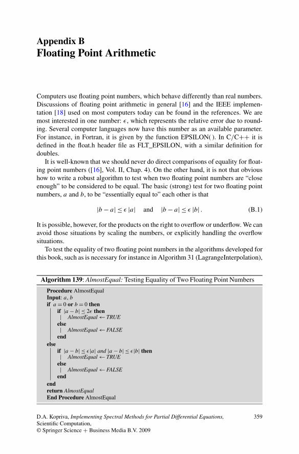
To test the equality of two floating point numbers in the algorithms developed forthis book, such as is necessary for instance in Algorithm 31 (LagrangeInterpolation),
Algorithm 139: AlmostEqual: Testing Equality of Two Floating Point Numbers
Procedure AlmostEqualInput: a, b
if a = 0 or b = 0 thenif |a − b| ≤ 2ε then
AlmostEqual ← TRUEelse
AlmostEqual ← FALSEend
elseif |a − b| ≤ ε|a| and |a − b| ≤ ε|b| then
AlmostEqual ← TRUEelse
AlmostEqual ← FALSEend
endreturn AlmostEqualEnd Procedure AlmostEqual
D.A. Kopriva, Implementing Spectral Methods for Partial Differential Equations,Scientific Computation,© Springer Science + Business Media B.V. 2009
359
360 B Floating Point Arithmetic
we propose Algorithm 139 (AlmostEqual). Note that we do not have to worry aboutall exceptional cases here, particularly since the numbers that we work with are in[−1,1] or [0,2π]. Thus, the only exceptional cases we need to deal with are nearthe origin.
Appendix CBasic Linear Algebra Subroutines (BLAS)
The BLAS provide standard building blocks to perform basic vector and matrixoperations. There are three levels of BLAS, with each level performing more andmore complex operations. The first level, BLAS Level 1, is a collection of routinesthat compute common operations such as the Euclidean norm, the dot product, andvector operations such as y = αx + y, known as AXPY. A PDF reference of theavailable routines, blasqr.pdf, can be found at http://www.netlib.org/blas/.
BLAS libraries are freely available on the web, for example at www.netlib.org,and specifically optimized versions are often included with commercial compilers.Furthermore, the ATLAS (Automatically Tuned Linear Algebra Software) libraryfound at http://math-atlas.sourceforge.net can be compiled to create a portably effi-cient BLAS library.
The BLAS routines are named with the format xNAME, where “x” denotesthe precision of the arithmetic, either “D” for double precision or “S” for single.(For many routines, complex or complex*16 versions are available with the prefixes“C” and “Z”, respectively.) For example, the single precision dot product is namedSDOT.
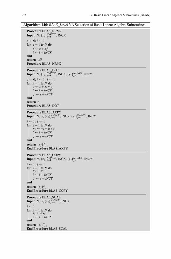
BLAS routines that are of use in this book include DOT, for the Euclidean innerproduct, NRM2, for the Euclidean norm, AXPY, for scalar times vector plus vector,COPY and SCAL. The standard calling arguments are
_DOT(N,X,INCX,Y,INCY)_NRM2(N,X,INCX)_AXPY(N,ALPHA,X,INCX,Y,INCY)_COPY(N,X,INCX,Y,INCY)_SCAL(N,ALPHA,X,INCX)
In each case, N corresponds to the total number of elements. The arguments X
and Y correspond to the input/output arrays. The integers INCX and INCY indi-cate the stride of the data, and enable the computation of subarray operations. Theargument ALPHA corresponds to the scalar parameter.
All arrays used in BLAS routines are constrained to be contiguous, a constraintthat should be observed when using languages that define arrays as arrays of point-ers. As such, the BLAS routines, now called the dense versions, don’t distinguishbetween inputs that represent one or two-dimensional arrays.
For completeness, and by way of example, we present prototype algorithms tocompute the dot product, the Euclidean norm, y = αx + y, copy, and scale by aparameter. In practice, one should use optimized library versions. Consistent withthe dense BLAS philosophy, we constrain the input arrays to be contiguous, so itdoes not matter whether arguments represent single or multidimensional arrays.
D.A. Kopriva, Implementing Spectral Methods for Partial Differential Equations,Scientific Computation,© Springer Science + Business Media B.V. 2009
361
362 C Basic Linear Algebra Subroutines (BLAS)
Algorithm 140: BLAS_Level1:A Selection of Basic Linear Algebra Subroutines
Procedure BLAS_NRM2Input: N , {xj }N∗INCX
j=1 , INCX
z ← 0; i ← 1for j = 1 to N do
z ← z + x2i
i ← i + INCXendreturn
√z
Procedure BLAS_NRM2
Procedure BLAS_DOTInput: N , {xj }N∗INCX
j=1 , INCX, {yj }N∗INCYj=1 , INCY
z ← 0; i ← 1; j ← 1for k = 1 to N do
z ← z + xi ∗ yj
i ← i + INCXj ← j + INCY
endreturn zProcedure BLAS_DOT
Procedure BLAS_AXPYInput: N , α, {xj }N∗INCX
j=1 , INCX, {yj }N∗INCYj=1 , INCY
i ← 1; j ← 1for k = 1 to N do
yj ← yj + α ∗ xi
i ← i + INCXj ← j + INCY
endreturn {yj }Nj=1End Procedure BLAS_AXPY
Procedure BLAS_COPYInput: N , {xj }N∗INCX
j=1 , INCX, {yj }N∗INCYj=1 , INCY
i ← 1; j ← 1for k = 1 to N do
yj ← xi
i ← i + INCXj ← j + INCY
endreturn {yj }Nj=1End Procedure BLAS_COPY
Procedure BLAS_SCALInput: N , α, {xj }N∗INCX
j=1 , INCX
i ← 1for k = 1 to N do
xi ← αxi
i ← i + INCXendreturn {xi}Ni=1End Procedure BLAS_SCAL
Appendix DLinear Solvers
Approximations of potential problems and implicit discretizations of time depen-dent partial differential equations lead to linear systems of equations to solve. Wesolve the systems either directly, typically by some variant of Gauss elimination,or iteratively. In this appendix, we motivate the algorithms that we use to solve thesystems that appear in this book. In no way can a short appendix like this surveythe entire field of numerical linear algebra and all the issues related to efficiency,parallelism, etc. For further study, we suggest the books [13] or [19].
D.1 Direct Solvers
For small enough systems, or in special cases, direct linear system solvers are ef-ficient. In this section, we discuss two, namely the Thomas algorithm to solvetri-diagonal systems, and LU factorization to solve full, general systems. In bothcases, well-tested and portable code with multiple language bindings is availablein the LAPACK [2] library. Some compiler vendors supply precompiled versionsof LAPACK, which should be used if possible. Otherwise, it is possible to down-load the source code from www.netlib.org (see, in particular, http://www.netlib.org/lapack/index.html) and compile it oneself.
D.1.1 Tri-Diagonal Solver
Tri-diagonal matrix problems are ubiquitous in numerical analysis, and appear, forexample in Sect. 4.5 with the Legendre Galerkin approximation. For completeness,therefore, we include the Thomas algorithm for the solution of tri-diagonal systems.We represent the elements of the matrix by the three vectors �, d and u, for thesubdiagonal, diagonal and superdiagonal elements, numbered as
⎡⎢⎢⎢⎢⎢⎢⎢⎣
d0 u0 0 . . . 0
�1 d1 u1. . .
...
0 �2 d2. . . 0
.... . .
. . . uN−10 . . . 0 �N dN
⎤⎥⎥⎥⎥⎥⎥⎥⎦
⎡⎢⎢⎢⎢⎢⎣
x0x1...
xN−1xN
⎤⎥⎥⎥⎥⎥⎦
=
⎡⎢⎢⎢⎢⎢⎣
y0y1...
yN−1yN
⎤⎥⎥⎥⎥⎥⎦
. (D.1)
D.A. Kopriva, Implementing Spectral Methods for Partial Differential Equations,Scientific Computation,© Springer Science + Business Media B.V. 2009
363
364 D Linear Solvers
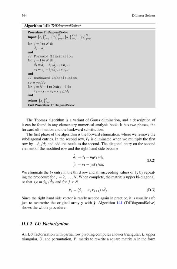
Algorithm 141: TriDiagonalSolve:
Procedure TriDiagonalSolve
Input:{�j
}N
j=1 ,{dj
}N
j=0 ,{uj
}N−1j=0 ,
{yj
}N
j=0
for j = 0 to N dodj = dj
end// Forward Eliminationfor j = 1 to N do
dj = dj − �j /dj−1 ∗ uj−1
yj = yj − �j /dj−1 ∗ yj−1
end// Backward Substitution
xN = yN/dN
for j = N − 1 to 0 step −1 doxj = (yj − uj ∗ xj+1)/dj
end
return{xj
}N
j=0End Procedure TriDiagonalSolve
The Thomas algorithm is a variant of Gauss elimination, and a description ofit can be found in any elementary numerical analysis book. It has two phases, theforward elimination and the backward substitution.
The first phase of the algorithm is the forward elimination, where we remove thesubdiagonal entries. In the second row, �1 is eliminated when we multiply the firstrow by −�1/d0 and add the result to the second. The diagonal entry on the secondelement of the modified row and the right hand side become
d1 = d1 − u0�1/d0,
y1 = y1 − y0�1/d0.(D.2)
We eliminate the �2 entry in the third row and all succeeding values of �j by repeat-ing the procedure for j = 2, . . . ,N . When complete, the matrix is upper bi-diagonal,so that xN = yN/dN and for j < N ,
xj = (yj − ujxj+1
)/dj . (D.3)
Since the right hand side vector is rarely needed again in practice, it is usually safejust to overwrite the original array y with y. Algorithm 141 (TriDiagonalSolve)shows the whole procedure.
D.1.2 LU Factorization
An LU factorization with partial row pivoting computes a lower triangular, L, uppertriangular, U , and permutation, P , matrix to rewrite a square matrix A in the form
D Linear Solvers 365
A = PLU . The permutation matrix is there to swap rows to ensure that the diagonalcontains the largest element in a column. The attraction of the algorithm is that oncewe compute and store the factorization, we solve the system Ax = y efficientlyfor multiple right hand sides, y, by a triangular forward substitution followed by atriangular backward substitution.
To motivate the algorithm, let’s assume that row swapping (pivoting) is notneeded. Then A = LU and we write the matrix multiplication component-wise as
aij =N∑
n=1
�inunj =min(i,j)∑
n=1
�inunj , (D.4)
since L is lower triangular and U is upper triangular. If we choose �kk = 1 (givingus what is known as the Doolittle Method), we can write
akj =k−1∑n=1
�knunj + ukj , j = k, . . . ,N,
aik =k−1∑n=1
�inunk + �ikukk, i = k + 1, . . . ,N.
(D.5)
We rearrange these to solve for the unknowns
ukj = akj −k−1∑n=1
�knunj , j = k, . . . ,N,
�ik = 1
ukk
(aik −
k−1∑n=1
�inunk
), i = k + 1, . . . ,N.
(D.6)
Typically, one destroys the original matrix by writing U to the upper triangular partof the A, and L to the lower. Since we chose the diagonal of L to be one, it doesn’tneed to be stored, which allows the diagonal part of U to be stored there instead.
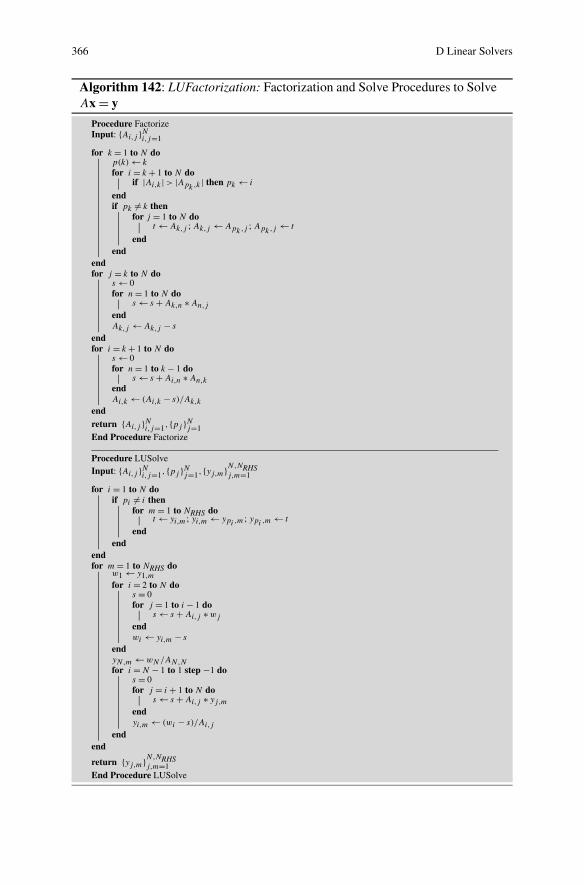
In general, we must swap rows to move the largest element in a row to the di-agonal. The information can be stored in a single pivot vector, {pj }Nj=1, that simplytells which row must be swapped with the current row. The procedure Factorize inAlgorithm 142 (LUFactorization) prototypes how to decompose a matrix into itsA = PLU factorization for columnwise storage of the matrix A. Note that this pro-cedure, like most library factorization procedures, destroys the original matrix tosave storage. An easy mistake to make is to forget and try to use the matrix againafter it has been factorized.
We break the solve operation into two steps. Since A = PLU ,
PLUx = y (D.7)
or
LUx = P y (D.8)
366 D Linear Solvers
Algorithm 142: LUFactorization: Factorization and Solve Procedures to SolveAx = y
Procedure FactorizeInput: {Ai,j }N
i,j=1
for k = 1 to N dop(k) ← k
for i = k + 1 to N doif |Ai,k | > |Apk,k | then pk ← i
endif pk �= k then
for j = 1 to N dot ← Ak,j ; Ak,j ← Apk,j ; Apk,j ← t
endend
endfor j = k to N do
s ← 0for n = 1 to N do
s ← s + Ak,n ∗ An,j
endAk,j ← Ak,j − s
endfor i = k + 1 to N do
s ← 0for n = 1 to k − 1 do
s ← s + Ai,n ∗ An,kendAi,k ← (Ai,k − s)/Ak,k
endreturn {Ai,j }N
i,j=1, {pj }Nj=1
End Procedure Factorize
Procedure LUSolveInput: {Ai,j }N
i,j=1, {pj }Nj=1, {yj,m}N,NRHS
j,m=1
for i = 1 to N doif pi �= i then
for m = 1 to NRHS dot ← yi,m ; yi,m ← ypi ,m
; ypi ,m← t
endend
endfor m = 1 to NRHS do
w1 ← y1,m
for i = 2 to N dos = 0for j = 1 to i − 1 do
s ← s + Ai,j ∗ wj
endwi ← yi,m − s
endyN,m ← wN /AN,Nfor i = N − 1 to 1 step −1 do
s = 0for j = i + 1 to N do
s ← s + Ai,j ∗ yj,m
endyi,m ← (wi − s)/Ai,j
endend
return {yj,m}N,NRHSj,m=1
End Procedure LUSolve
D Linear Solvers 367
since swapping a row then swapping again returns rows to their original state andimplies P −1 = P . If we define w = Ux, we can solve two triangular systems insuccession
Lw = P y,
Ux = w.(D.9)
The first is simply forward substitution. Since
i∑j=1
Lijwj = (Py)i , (D.10)
we solve w1 = (Py)1/L11 = (Py)1 and
wi = (Py)i −i−1∑j=1
Lijwj , i = 2,3, . . . ,N. (D.11)
We derive a similar back substitution formula to solve Ux = w. The combinationof these two form the LUSolve procedure in Algorithm 142 (LUFactorization). Theinput to the procedure is the factorized matrix, i.e. the output of Factorize. To ac-commodate multiple right hand sides, we assume that a two dimensional array withNRHS columns is supplied, as is done with the LAPACK routines. The output is thenan array whose columns are the solution vector for each right hand side.
Rather than use these prototype procedures in production, which we present hereto understand how the algorithm works, it is better to use optimized library routinessuch as those provided by LAPACK [2]. The LAPACK routines can take advan-tage of optimized BLAS routines and run efficiently on parallel systems. The tworoutines useful for general matrices are
xGETRF(M, N, A, LDA, IPIV, INFO)xGETRS(TRANS, N, NRHS, A, LDA, IPIV, B, LDB, INFO)
where “x” denotes the data type of the variables, “D” for double, “S” for single, forinstance. The procedures perform the factorization (F) and Solve (S) phases sepa-rately. The arguments are the number of rows and columns, M and N, the matrix A,the leading dimension of A, LDA, the pivot vector, IPIV and an error flag. The solveroutine takes a character variable, TRANS, that specifies if the transpose of A is tobe used. The argument N is the order of the matrix A and NRHS is NRHS. Thenext three arguments are the same as for xGETRF, but A is the factorized matrix.Finally, B corresponds to {yj,m}N,NRHS
j,m=1 where LDB is the leading dimension of thearray B.
368 D Linear Solvers
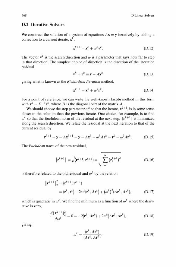
D.2 Iterative Solvers
We construct the solution of a system of equations Ax = y iteratively by adding acorrection to a current iterate, xk ,
xk+1 = xk + ωkvk. (D.12)
The vector vk is the search direction and ω is a parameter that says how far to stepin that direction. The simplest choice of direction is the direction of the iterationresidual
vk = rk ≡ y − Axk (D.13)
giving what is known as the Richardson Iteration method,
xk+1 = xk + ωkrk. (D.14)
For a point of reference, we can write the well-known Jacobi method in this formwith vk = D−1rk , where D is the diagonal part of the matrix A.
We should choose the step parameter ωk so that the iterate, xk+1, is in some sensecloser to the solution than the previous iterate. One choice, for example, is to findωk so that the Euclidean norm of the residual at the next step, ‖rk+1‖ is minimizedalong the search direction. We relate the residual at the next iteration to that of thecurrent residual by
rk+1 = y − Axk+1 = y − Axk − ωkArk = rk − ωkArk. (D.15)
The Euclidean norm of the new residual,
∥∥rk+1∥∥ =
√⟨rk+1, rk+1
⟩ =√√√√ N∑
i=1
(rk+1i
)2 (D.16)
is therefore related to the old residual and ωk by the relation
∥∥rk+1∥∥2
2 = ⟨rk+1, rk+1⟩
= ⟨rk, rk
⟩ − 2ωk⟨rk,Ark
⟩ + (ωk
)2⟨Ark,Ark
⟩, (D.17)
which is quadratic in ωk . We find the minimum as a function of ωk where the deriv-ative is zero,
d‖rk+1‖22
dωk= 0 = −2
⟨rk,Ark
⟩ + 2ωk⟨Ark,Ark
⟩, (D.18)
giving
ωk = 〈rk,Ark〉〈Ark,Ark〉 . (D.19)
D Linear Solvers 369
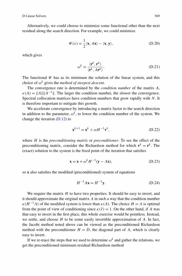
Alternatively, we could choose to minimize some functional other than the nextresidual along the search direction. For example, we could minimize
Ψ (x) = 1
2〈x,Ax〉 − 〈x,y〉, (D.20)
which gives
ωk = 〈rk, rk〉〈rk,Ark〉 . (D.21)
The functional Ψ has as its minimum the solution of the linear system, and thischoice of ωk gives the method of steepest descent.
The convergence rate is determined by the condition number of the matrix A,κ(A) = ‖A‖‖A−1‖. The larger the condition number, the slower the convergence.Spectral collocation matrices have condition numbers that grow rapidly with N . Itis therefore important to mitigate this growth.
We accelerate convergence by introducing a matrix factor to the search directionin addition to the parameter, ωk , to lower the condition number of the system. Wechange the iteration (D.12) to
xk+1 = xk + ωH−1vk, (D.22)
where H is the preconditioning matrix or preconditioner. To see the effect of thepreconditioning matrix, consider the Richardson method for which vk = rk . The(exact) solution to the system is the fixed point of the iteration that satisfies
x = x + ωkH−1(y − Ax), (D.23)
so x also satisfies the modified (preconditioned) system of equations
H−1Ax = H−1y. (D.24)
We require the matrix H to have two properties: It should be easy to invert, andit should approximate the original matrix A in such a way that the condition numberκ(H−1A) of the modified system is lower than κ(A). The choice H = A is optimalfrom the point of view of conditioning since κ(I ) = 1. On the other hand, if A wasthat easy to invert in the first place, this whole exercise would be pointless. Instead,we settle, and choose H to be some easily invertible approximation of A. In fact,the Jacobi method noted above can be viewed as the preconditioned Richardsonmethod with the preconditioner H = D, the diagonal part of A, which is clearlyeasy to invert.
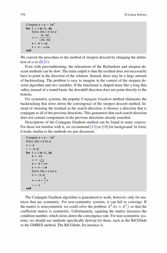
If we re-trace the steps that we used to determine ωk and gather the relations, weget the preconditioned minimum residual Richardson method
370 D Linear Solvers
Compute r = y − Ax0
for k = 1 to Nit doSolve Hz = r for z
ω ← 〈r,Az〉〈Az,Az〉
x ← x + ωzr ← r − ωAz
end
We convert the procedure to the method of steepest descent by changing the defini-tion of ω to (D.21).
Even with preconditioning, the relaxations of the Richardson and steepest de-scent methods can be slow. The main culprit is that the residual does not necessarilyhave to point in the direction of the solution. Instead, there may be a large amountof backtracking. The problem is easy to imagine in the context of the steepest de-scent algorithm and two variables. If the functional is shaped more like a long thinvalley instead of a round basin, the downhill direction does not point directly to thebottom.
For symmetric systems, the popular Conjugate Gradient method eliminates thebacktracking that slows down the convergence of the steepest descent method. In-stead of choosing the residual as the search direction, it chooses a direction that isconjugate to all of the previous directions. This guarantees that each search directiondoes not contain components in the previous directions already searched.
Descriptions of the Conjugate Gradient method can be found in many sources.For those not familiar with it, we recommend [13] or [19] for background. In form,it looks similar to the methods we just discussed,
Compute r = y − Ax0
Solve Hz = r for zv ← zc ← 〈r, z〉for k = 1 to Nit do
z ← Avω ← c
〈v,z〉x ← x + ωvr ← r − ωzSolve Hz = r for zd ← 〈r, z〉v ← z + d
cv
c ← dend
The Conjugate Gradient algorithm is guaranteed to work, however, only for ma-trices that are symmetric. For non-symmetric systems, it can fail to converge. Ifthe matrix is nonsymmetric we could solve the problem AT Ax = AT y so that thecoefficient matrix is symmetric. Unfortunately, squaring the matrix increases thecondition number, which slows down the convergence rate. For non-symmetric sys-tems, we should use methods specifically derived for them, such as the BiCGStabor the GMRES method. The BiCGStab, for instance is
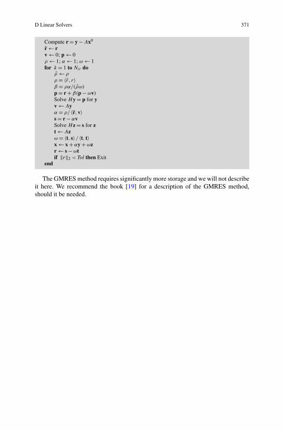
D Linear Solvers 371
Compute r = y − Ax0
r ← rv ← 0; p ← 0ρ ← 1; α ← 1; ω ← 1for k = 1 to Nit do
ρ ← ρ
ρ = 〈r , r〉β = ρα/(ρω)
p = r + β(p − ωv)
Solve Hy = p for yv ← Ayα = ρ/ 〈r,v〉s = r − αvSolve Hz = s for zt ← Azω = 〈t, s〉/ 〈t, t〉x ← x + αy + ωzr ← s − ωtif ‖r‖2 < Tol then Exit
end
The GMRES method requires significantly more storage and we will not describeit here. We recommend the book [19] for a description of the GMRES method,should it be needed.
Appendix EData Structures
Arrays have both advantages and disadvantages as structures in which to store data.Their main advantage, beyond their simplicity, is that operations on arrays can becomputed very efficiently. Standardization of such operations has led to the basiclinear algebra subroutines (BLAS) that we discussed in Appendix C. Also, accessto a particular element of an array is fast. The main disadvantage, which goes handin hand with simplicity and efficiency, is that arrays are not very flexible. For bestefficiency, we typically must fix the size of an array. If we don’t know the sizebeforehand, the addition of new elements or the deletion of existing elements canrequire costly allocation and deallocation of blocks of memory, plus the time tocopy data from old to new versions of the array. To enable flexible data storage andretrieval, we need more sophisticated data structures.
In this appendix we describe two useful data structures. The first is the linkedlist. In contrast to arrays, linked lists do not have a specified ordering of the data.They have the advantage that we can easily add and delete elements of the list, so wedon’t have to know the size of a list in advance. On the negative side, because thereis no structured ordering of the data, it is expensive to find a particular element ofa list. The second data structure is the hash table. Hash tables are flexible structuresthat are efficient to search.
Our discussion of data structures will be necessarily brief, and we will discussonly aspects that we need to implement the spectral element algorithms in this book.In particular, our discussion of hash tables is limited to an example of a sparsematrix. Further discussion of the subject of data structures can be found in manybooks, such as that of Knuth [16]. Note that it is particularly easy to find detaileddiscussions of linked lists, since they are often used in programming language booksfor examples of how to use pointers.
E.1 Linked Lists
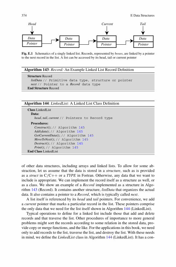
A linked list is a data structure that consists of a collection of records. In a singlylinked list, the record consists of two parts, namely the data that it holds and a pointerto the next record. (Variations that we do not need to consider here include doublylinked lists where a record also has a pointer to the previous record, and circularlylinked lists whose last record points to the first record of the list.) We show a diagramof a singly linked list in Fig. E.1.
The records linked in a singly linked list data structure contain data and a pointer(or pointers) to other records. The data stored in the record can be something assimple as an integer value, or as complicated as a structure that contains a variety
D.A. Kopriva, Implementing Spectral Methods for Partial Differential Equations,Scientific Computation,© Springer Science + Business Media B.V. 2009
373
374 E Data Structures
Fig. E.1 Schematics of a singly linked list. Records, represented by boxes, are linked by a pointerto the next record in the list. A list can be accessed by its head, tail or current pointer
Algorithm 143: Record: An Example Linked List Record Definition
Structure RecordlistData // Primitive data type, structure or pointernext // Pointer to a Record data type
End Structure Record
Algorithm 144: LinkedList: A Linked List Class Definition
Class LinkedListData:
head, tail, current // Pointers to Record type
Procedures:Construct(); // Algorithm 145Add(data); // Algorithm 145GetCurrentData(); // Algorithm 145MoveToNext(); // Algorithm 145Destruct(); // Algorithm 145Print(); // Algorithm 145
End Class LinkedList
of other data structures, including arrays and linked lists. To allow for some ab-straction, let us assume that the data is stored in a structure, such as is providedas a struct in C/C++ or a TYPE in Fortran. Otherwise, any data that we want toinclude is appropriate. We can implement the record itself as a structure as well, oras a class. We show an example of a Record implemented as a structure in Algo-rithm 143 (Record). It contains another structure, listData that organizes the actualdata. It also contains a pointer to a Record, which is typically called next.
A list itself is referenced by its head and tail pointers. For convenience, we adda current pointer that marks a particular record in the list. These pointers comprisethe only data that we need for the list itself shown in Algorithm 144 (LinkedList).
Typical operations to define for a linked list include those that add and deleterecords and that traverse the list. Other procedures of importance to more generalproblems might sort the records according to some relation in the stored data, pro-vide copy or merge functions, and the like. For the applications in this book, we needonly to add records to the list, traverse the list, and destroy the list. With these needsin mind, we define the LinkedList class in Algorithm 144 (LinkedList). It has a con-
E Data Structures 375
Algorithm 145: LinkedList:Procedures:
Procedure Construct
this.head ⇒ NULLthis.tail ⇒ NULLthis.current ⇒ NULLEnd Procedure Construct
Procedure AddInput: data // is either a primitive, a structure, or a pointer
Allocate newRecordif this.tail ⇒ NULL then
this.head ⇒ newRecordthis.tail ⇒ newRecord
elsethis.tail.next ⇒ newRecordthis.tail ⇒ newRecord
endthis.current ⇒ this.tailthis.current.next ⇒ NULLthis.current.listData ← dataEnd Procedure Add
Procedure GetCurrentDatareturn this.current.listDataEnd Procedure GetCurrentData
Procedure MoveToNextthis.current ⇒ this.current.nextEnd Procedure MoveToNext
Procedure Destructthis.current ⇒ this.headwhile this.current �⇒ NULL do
pNext ⇒ this.current.nextDeallocate memory pointed to by this.currentthis.current ⇒ pNext
endEnd Procedure Destruct
Procedure Printthis.current ⇒ this.headwhile this.current �⇒ NULL do
Print this.current.datathis.MoveToNext()
endEnd Procedure Print
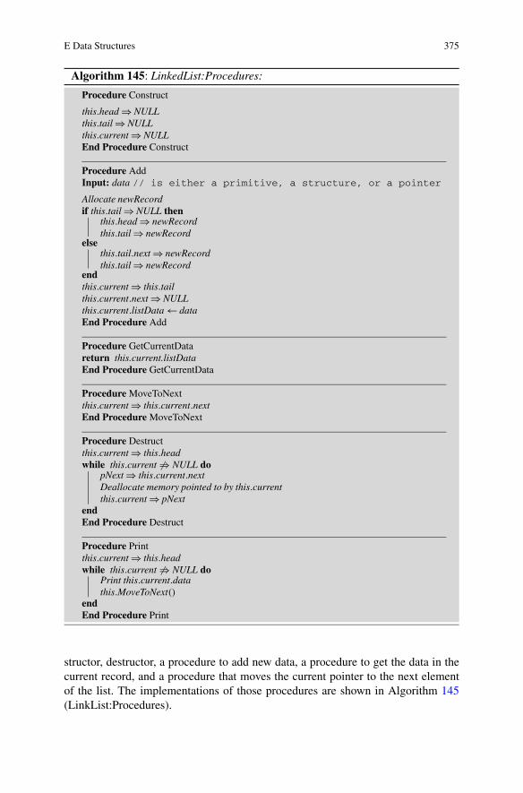
structor, destructor, a procedure to add new data, a procedure to get the data in thecurrent record, and a procedure that moves the current pointer to the next elementof the list. The implementations of those procedures are shown in Algorithm 145(LinkList:Procedures).
376 E Data Structures
The constructor for the linked list in Algorithm 145 (LinkList:Procedures) haslittle to do. It simply sets the pointers to point to NULL, which denotes that thepointer does not yet point to any record.
The Add procedure takes data as input, creates (allocates) a pointer to a newrecord and adds the new record to the end of the list, if the list is not empty. Ifthe list is empty, then the new record becomes the start of the list and all the list’spointers point to it.
The MoveToNext and Destruct procedures illustrate how to navigate the list. Tomove one step from any position in the list, the current pointer is pointed to it’snext pointer. The Destruct procedure shows how to navigate through the entire list.There, we set a pointer to the head and another to its next pointer (to keep the nextrecord accessible). A while loop then steps through the entire list until the end, whichis detected by the current pointer pointing to NULL. At each step, the memory towhich the current record points is destroyed, and the current pointer is set to pointto what was the next record in the list.
We could construct new procedures to perform whole list actions, such asprinting the list or searching for a record whose data matches a given criterion,by modifying the Destruct procedure. The Print procedure in Algorithm 145(LinkList:Procedures), for instance, loops through the list and prints the data as-sociated with the record pointed to by the current pointer. To search for a recordwith particular data, we would replace the print line in the Print procedure with atest on the data.
The Add and Delete procedures illustrate the flexibility of a linked list to storedata when we do not know the number of records ahead of time. The Destruct andPrint procedures show the weakness of a linked list. To access a particular record,we must start at the beginning and search for it sequentially. There is no mechanismfor random access to the records, say, to access the fifth element directly, as can bedone with an array. Neither can the list find a particular record with a given datavalue without stepping through the list from the beginning.
E.1.1 Example: Elements that Share a Node
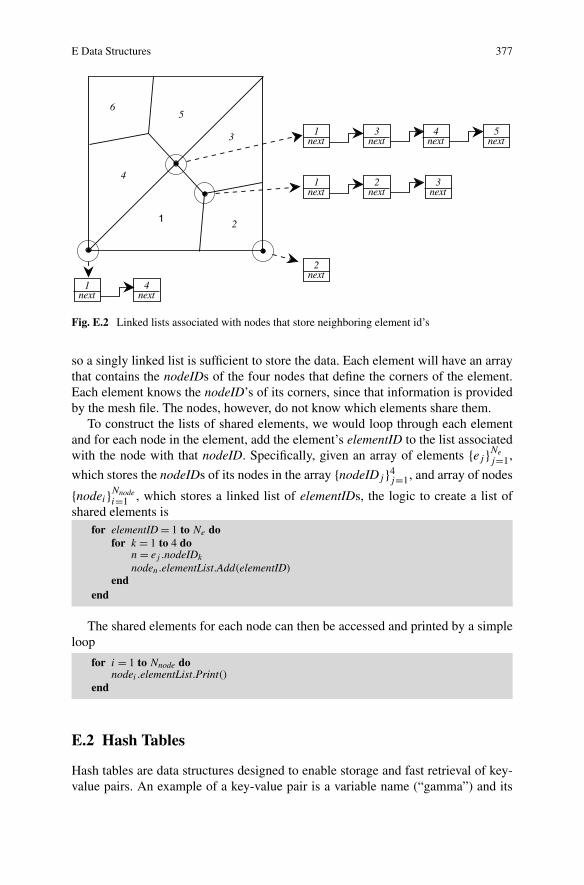
One example of where a linked list is useful is to collect the id’s of all the spectralelements in a mesh that share a common corner node. In a structured mesh, a nodemight be shared by one, two or four elements. In an unstructured mesh a node mayin principle be shared by any number of elements (Fig. E.2). Operations on each listare typically of a “ForAll” type, so the entire list must be traversed, but the order inwhich elements are accessed is not often important. For these needs, a linked list isappropriate to store the shared elementID’s for each node.
Let us assume that we have an array of nodes stored by their nodeID, and anarray of elements stored by their elementID. We create such arrays by reading theinformation from a data file created by a mesh generator. Each node will store (in ad-dition to its other data, such as location) a linked list whose data is just an elementID(Fig. E.2). We will not need to modify this shared element data after it is created,
E Data Structures 377
Fig. E.2 Linked lists associated with nodes that store neighboring element id’s
so a singly linked list is sufficient to store the data. Each element will have an arraythat contains the nodeIDs of the four nodes that define the corners of the element.Each element knows the nodeID’s of its corners, since that information is providedby the mesh file. The nodes, however, do not know which elements share them.
To construct the lists of shared elements, we would loop through each elementand for each node in the element, add the element’s elementID to the list associatedwith the node with that nodeID. Specifically, given an array of elements {ej }Ne
j=1,
which stores the nodeIDs of its nodes in the array {nodeIDj }4j=1, and array of nodes
{nodei}Nnodei=1 , which stores a linked list of elementIDs, the logic to create a list of
shared elements isfor elementID = 1 to Ne do
for k = 1 to 4 don = ej .nodeIDk
noden.elementList.Add(elementID)end
end
The shared elements for each node can then be accessed and printed by a simpleloop
for i = 1 to Nnode donodei .elementList.Print()
end
E.2 Hash Tables
Hash tables are data structures designed to enable storage and fast retrieval of key-value pairs. An example of a key-value pair is a variable name (“gamma”) and its
378 E Data Structures
associated value (“1.4”). The table itself is typically an array. The location of thevalue in a hash table associated with a key, k, is specified by way of a hash func-tion, H(k). In the case of a variable name and value, the hash function convertsthe name into an integer that tells it where to find the associated value in the ta-ble.
A very simple example of a hash table is, in fact, a singly dimensioned array. Thekey is the array index and the value is what is stored at that index. Multiple keys canbe used to identify data; a two dimensional array provides an example where twokeys are used to access memory and retrieve the value at that location. If we viewa singly dimensioned array as a special case of a hash table, its hash function isjust the array index, H(j) = j . A doubly dimensioned array could be (and often is)stored columnwise as a singly dimensioned array by creating a hash function thatmaps the two indices to a single location in the array, e.g., H(i, j) = i + j ∗ N ,where N is the range of the first index, i.
Although arrays provide fast access to their data, they allocate storage for allpossible keys, and only set the value for a key if the data associated with a particularkey is present. A matrix, for instance, can be stored as a two-dimensional array.The value of the (i, j)th element of the matrix is stored at a location in memoryassociated with the two keys, (i, j). A sparse matrix can require much more memorythan necessary when stored this way, since most of the elements are zero and don’tneed to be stored at all. It is for sparse data structures like this that hash tables areuseful.
To create a hash table, we need a storage model and a hash function. Each haspractical issues. Often it is convenient and efficient to store the data in an arrayof fixed size. The hash function will then map the keys to an element of that array.However, when we are done, we want that array to be fully populated so that there isno wasted space. Therefore, we don’t want to allocate an array that can hold all pos-sible values for all possible keys (as in the matrix storage problem above), only onesthat can hold the values for keys that occur. It is not generally desirable to create a“perfect” hash function that generates a unique index for a given set of keys. In-stead, collisions will be allowed where different keys can give the same hash value,i.e., point to the same location in the array. For instance, it is unrealistic to create adictionary (word + definition) by allocating storage for every possible combinationof letters. Instead we might define a finite array and create a hash function to map tothat array. We could create the hash function by assigning a value to each letter, likeits position in the alphabet, and adding the values in the word. Thus the word “dad”would be hashed to index 4 + 1 + 4 = 9. But so would “fab”.
Of the many ways to resolve collisions, chaining is common. To use chaining,each entry in the array stores a pointer to a linked list, instead of storing values inthe hash table array itself. As collisions occur, the new entry is added to the linkedlist. Then, when it is time to retrieve the value associated with a key, the key ishashed and the linked list at the location given by the hash value is then searched(sequentially) for the actual key. Yes, we have already said that it is slow to search alinked list. But if the table is of a reasonable size, and the hash function is reasonable,then the number of collisions, and hence the number of entries in the linked list, willbe small and quickly searched.
E Data Structures 379
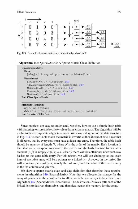
Fig. E.3 Example of sparse matrix representation by a hash table
Algorithm 146: SparseMatrix: A Sparse Matrix Class Definition
Class SparseMatrixData:
{tablei} // Array of pointers to LinkedList
Procedures:Construct(N) ; // Algorithm 147AddDataForKeys(data, i, j); // Algorithm 147DataForKeys(i, j); // Algorithm 147ContainsKeys(i, j); // Algorithm 147Destruct(); // Algorithm 147
End Class SparseMatrix
Structure TableDatakey // an integerdata // a primitive type, structure, or pointer
End Structure TableData
Since matrices are easy to understand, we show how to use a simple hash tablewith chaining to store and retrieve values from a sparse matrix. The algorithm will beuseful to delete duplicate edges in a mesh. We show a diagram of the data structurein Fig. E.3. To start, note that if the matrix is invertible, then it cannot have a row thatis all zeros, that is, every row must have at least one entry. Therefore, the table itselfshould be an array of length N , where N is the order of the matrix. Each location inthe table will correspond to a row in the matrix and the hash function for a matrixelement (i, j) is simply H(i, j) = i. Clearly there will be collisions, since each rowhashes to the same table entry. For this reason, we will use chaining so that eachitem of the table array will be a pointer to a linked list. A record in the linked listwill store two pieces of data, namely the column j and the value of the matrix entryin the ith column and j th row.
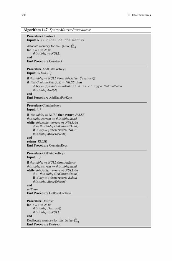
We show a sparse matrix class and data definition that describe these require-ments in Algorithm 146 (SparseMatrix). Note that we allocate the storage for thearray of pointers in the constructor to allow variable size arrays to be created, seeAlgorithm 147 (SparseMatrix:Procedures). The destructor, Destruct tells each of thelinked lists to destruct themselves and then deallocates the memory for the array.
380 E Data Structures
Algorithm 147: SparseMatrix:Procedures:
Procedure ConstructInput: N // Order of the matrix
Allocate memory for this. {tablei}Ni=1for i = 1 to N do
this.tablei ⇒ NULLendEnd Procedure Construct
Procedure AddDataForKeysInput: inData, i, j
if this.tablei ⇒ NULL then this.tablei .Construct()if this.ContainsKeys(i, j) = FALSE then
d.key ← j ;d.data ← inData // d is of type TableDatathis.tablei .Add(d)
endEnd Procedure AddDataForKeys
Procedure ContainsKeysInput: i, j
if this.tablei ⇒ NULL then return FALSEthis.tablei .current ⇒ this.tablei .headwhile this.tablei .current �⇒ NULL do
d ← this.tablei .GetCurrentData()
if d.key = j then return TRUEthis.tablei .MoveToNext()
endreturn FALSEEnd Procedure ContainsKeys
Procedure GetDataForKeysInput: i, j
if this.tablei ⇒ NULL then setErrorthis.tablei .current ⇒ this.tablei .headwhile this.tablei .current �⇒ NULL do
d ← this.tablei .GetCurrentData()
if d.key = j then return d.datathis.tablei .MoveToNext()
endsetErrorEnd Procedure GetDataForKeys
Procedure Destructfor i = 1 to N do
this.tablei .Destruct()this.tablei ⇒ NULL
endDeallocate memory for this. {tablei}Ni=1End Procedure Destruct
E Data Structures 381
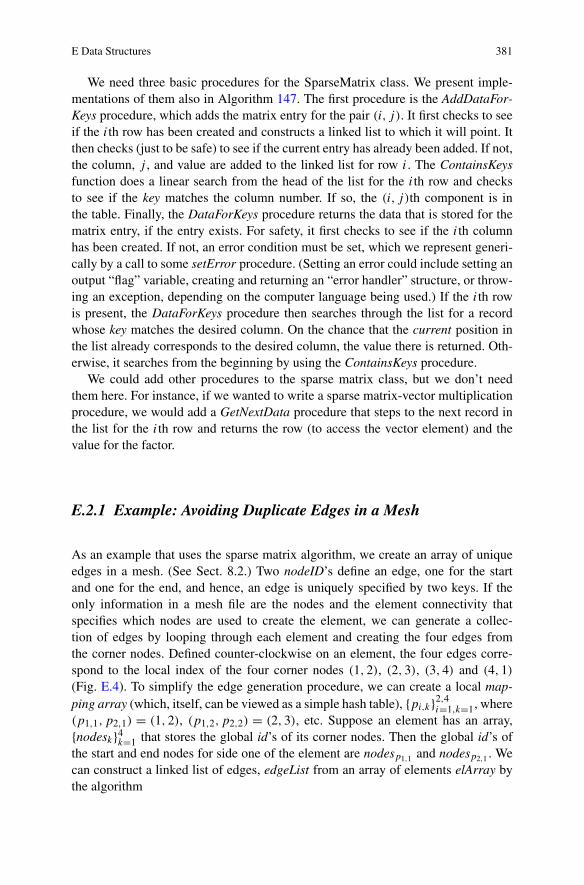
We need three basic procedures for the SparseMatrix class. We present imple-mentations of them also in Algorithm 147. The first procedure is the AddDataFor-Keys procedure, which adds the matrix entry for the pair (i, j). It first checks to seeif the ith row has been created and constructs a linked list to which it will point. Itthen checks (just to be safe) to see if the current entry has already been added. If not,the column, j , and value are added to the linked list for row i. The ContainsKeysfunction does a linear search from the head of the list for the ith row and checksto see if the key matches the column number. If so, the (i, j)th component is inthe table. Finally, the DataForKeys procedure returns the data that is stored for thematrix entry, if the entry exists. For safety, it first checks to see if the ith columnhas been created. If not, an error condition must be set, which we represent generi-cally by a call to some setError procedure. (Setting an error could include setting anoutput “flag” variable, creating and returning an “error handler” structure, or throw-ing an exception, depending on the computer language being used.) If the ith rowis present, the DataForKeys procedure then searches through the list for a recordwhose key matches the desired column. On the chance that the current position inthe list already corresponds to the desired column, the value there is returned. Oth-erwise, it searches from the beginning by using the ContainsKeys procedure.
We could add other procedures to the sparse matrix class, but we don’t needthem here. For instance, if we wanted to write a sparse matrix-vector multiplicationprocedure, we would add a GetNextData procedure that steps to the next record inthe list for the ith row and returns the row (to access the vector element) and thevalue for the factor.
E.2.1 Example: Avoiding Duplicate Edges in a Mesh
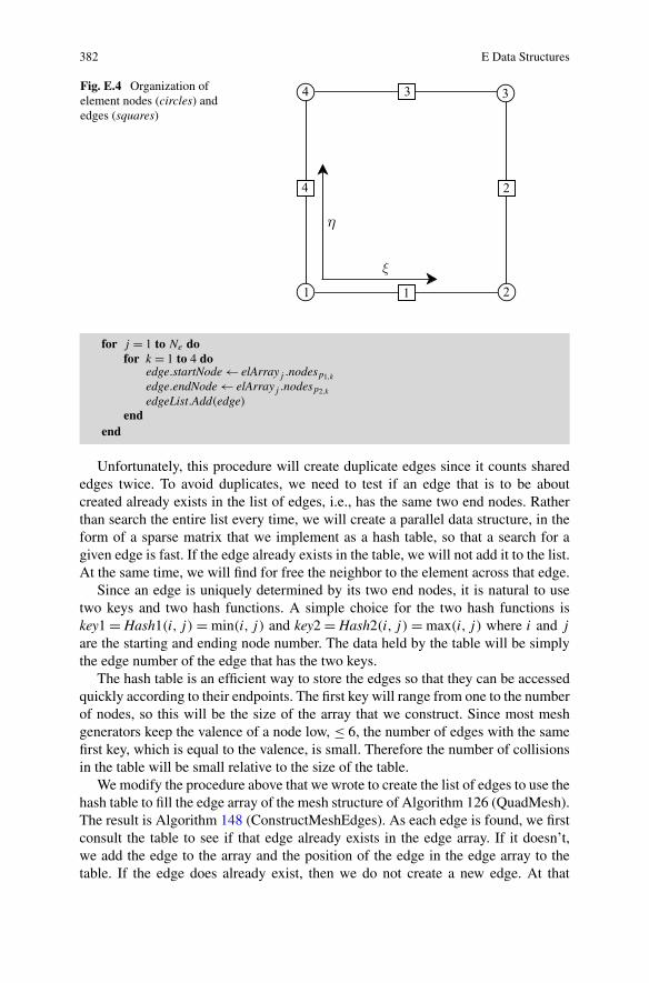
As an example that uses the sparse matrix algorithm, we create an array of uniqueedges in a mesh. (See Sect. 8.2.) Two nodeID’s define an edge, one for the startand one for the end, and hence, an edge is uniquely specified by two keys. If theonly information in a mesh file are the nodes and the element connectivity thatspecifies which nodes are used to create the element, we can generate a collec-tion of edges by looping through each element and creating the four edges fromthe corner nodes. Defined counter-clockwise on an element, the four edges corre-spond to the local index of the four corner nodes (1,2), (2,3), (3,4) and (4,1)
(Fig. E.4). To simplify the edge generation procedure, we can create a local map-ping array (which, itself, can be viewed as a simple hash table), {pi,k}2,4
i=1,k=1, where(p1,1,p2,1) = (1,2), (p1,2,p2,2) = (2,3), etc. Suppose an element has an array,{nodesk}4
k=1 that stores the global id’s of its corner nodes. Then the global id’s ofthe start and end nodes for side one of the element are nodesp1,1 and nodesp2,1 . Wecan construct a linked list of edges, edgeList from an array of elements elArray bythe algorithm
382 E Data Structures
Fig. E.4 Organization ofelement nodes (circles) andedges (squares)
for j = 1 to Ne dofor k = 1 to 4 do
edge.startNode ← elArrayj .nodesp1,k
edge.endNode ← elArrayj .nodesp2,k
edgeList.Add(edge)end
end
Unfortunately, this procedure will create duplicate edges since it counts sharededges twice. To avoid duplicates, we need to test if an edge that is to be aboutcreated already exists in the list of edges, i.e., has the same two end nodes. Ratherthan search the entire list every time, we will create a parallel data structure, in theform of a sparse matrix that we implement as a hash table, so that a search for agiven edge is fast. If the edge already exists in the table, we will not add it to the list.At the same time, we will find for free the neighbor to the element across that edge.
Since an edge is uniquely determined by its two end nodes, it is natural to usetwo keys and two hash functions. A simple choice for the two hash functions iskey1 = Hash1(i, j) = min(i, j) and key2 = Hash2(i, j) = max(i, j) where i and j
are the starting and ending node number. The data held by the table will be simplythe edge number of the edge that has the two keys.
The hash table is an efficient way to store the edges so that they can be accessedquickly according to their endpoints. The first key will range from one to the numberof nodes, so this will be the size of the array that we construct. Since most meshgenerators keep the valence of a node low, ≤ 6, the number of edges with the samefirst key, which is equal to the valence, is small. Therefore the number of collisionsin the table will be small relative to the size of the table.
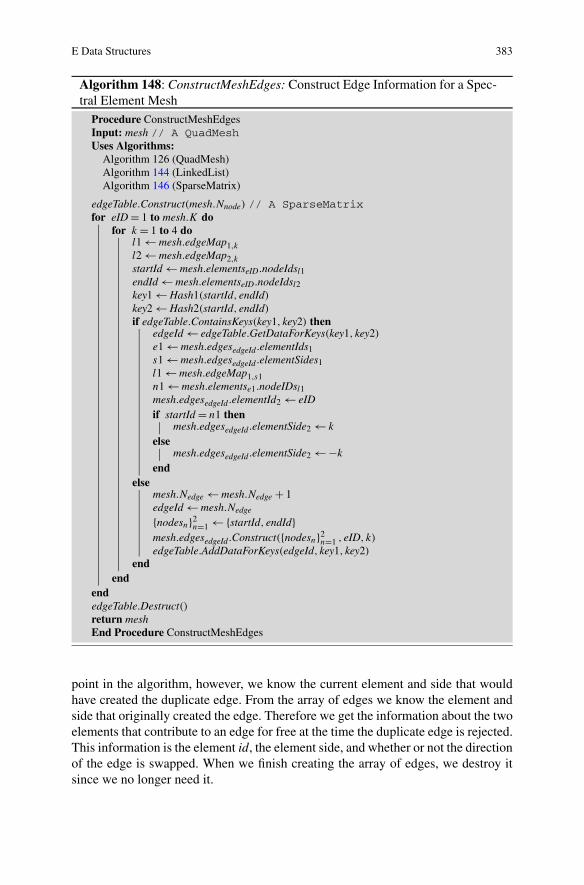
We modify the procedure above that we wrote to create the list of edges to use thehash table to fill the edge array of the mesh structure of Algorithm 126 (QuadMesh).The result is Algorithm 148 (ConstructMeshEdges). As each edge is found, we firstconsult the table to see if that edge already exists in the edge array. If it doesn’t,we add the edge to the array and the position of the edge in the edge array to thetable. If the edge does already exist, then we do not create a new edge. At that
E Data Structures 383
Algorithm 148: ConstructMeshEdges: Construct Edge Information for a Spec-tral Element Mesh
Procedure ConstructMeshEdgesInput: mesh // A QuadMeshUses Algorithms:
Algorithm 126 (QuadMesh)Algorithm 144 (LinkedList)Algorithm 146 (SparseMatrix)
edgeTable.Construct(mesh.Nnode) // A SparseMatrixfor eID = 1 to mesh.K do
for k = 1 to 4 dol1 ← mesh.edgeMap1,k
l2 ← mesh.edgeMap2,k
startId ← mesh.elementseID.nodeIdsl1endId ← mesh.elementseID.nodeIdsl2key1 ← Hash1(startId, endId)
key2 ← Hash2(startId, endId)
if edgeTable.ContainsKeys(key1, key2) thenedgeId ← edgeTable.GetDataForKeys(key1, key2)
e1 ← mesh.edgesedgeId.elementIds1s1 ← mesh.edgesedgeId.elementSides1l1 ← mesh.edgeMap1,s1n1 ← mesh.elementse1.nodeIDsl1mesh.edgesedgeId.elementId2 ← eIDif startId = n1 then
mesh.edgesedgeId.elementSide2 ← k
elsemesh.edgesedgeId.elementSide2 ← −k
endelse
mesh.Nedge ← mesh.Nedge + 1edgeId ← mesh.Nedge
{nodesn}2n=1 ← {startId, endId}
mesh.edgesedgeId.Construct({nodesn}2n=1 , eID, k)
edgeTable.AddDataForKeys(edgeId, key1, key2)
endend
endedgeTable.Destruct()return meshEnd Procedure ConstructMeshEdges
point in the algorithm, however, we know the current element and side that wouldhave created the duplicate edge. From the array of edges we know the element andside that originally created the edge. Therefore we get the information about the twoelements that contribute to an edge for free at the time the duplicate edge is rejected.This information is the element id, the element side, and whether or not the directionof the edge is swapped. When we finish creating the array of edges, we destroy itsince we no longer need it.
References
1. Abramowitz, M., Stegun, I.A.: Handbook of Mathematical Functions: with Formulas, Graphs,and Mathematical Tables. Dover, New York (1965)
2. Anderson, E., Bai, Z., Bischof, C., Blackford, S., Demmel, J., Dongarra, J., Croz, J.D., Green-baum, A., Hammarling, S., McKenney, A., Sorensen, D.: LAPACK Users’ Guide, 3rd edn.SIAM, Philadelphia (1999)
3. Ascher, U.M., Petzold, L.R.: Computer Methods for Ordinary Differential Equations andDifferential-Algebraic Equations. SIAM, Philadelphia (1998)
4. Boyd, J.P.: Chebyshev and Fourier Spectral Methods, 2nd revised edn. Dover, New York(2001)
5. Bracewell, R.: The Fourier Transform and Its Applications. McGraw-Hill, New York (1999)6. Brigham, E.: Fast Fourier Transform and Its Applications. Prentice Hall, New York (1988)7. Canuto, C., Hussaini, M., Quarteroni, A., Zang, T.: Spectral Methods: Fundamentals in Single
Domains. Springer, Berlin (2006)8. Canuto, C., Hussaini, M., Quarteroni, A., Zang, T.: Spectral Methods: Evolution to Complex
Geometries and Applications to Fluid Dynamics. Springer, Berlin (2007)9. Deville, M., Fischer, P., Mund, E.: High Order Methods for Incompressible Fluid Flow. Cam-
bridge University Press, Cambridge (2002)10. Don, W.S., Solomonoff, A.: Accuracy and speed in computing the Chebyshev collocation
derivative. SIAM J. Sci. Comput. 16, 1253–1268 (1995)11. Farrashkhalvat, M., Miles, J.P.: Basic Structured Grid Generation: With an Introduction to
Unstructured Grid Generation. Butterworth-Heinemann, Stoneham (2003)12. Frigo, M., Johnson, S.G.: The design and implementation of FFTW3. Proc. IEEE 93(2), 216–
231 (2005)13. Golub, G.H., Loan, C.F.V.: Matrix Computations. Johns Hopkins University Press, Baltimore
(1996)14. Hesthaven, J.S., Gottlieb, S., Gottlieb, D.: Spectral Methods for Time-Dependent Problems.
Cambridge University Press, Cambridge (2007)15. Knupp, P.M., Steinberg, S.: Fundamentals of Grid Generation. CRC Press, Boca Raton (1993)16. Knuth, D.E.: The Art of Computer Programming. Addison-Wesley, Reading (1998)17. Lambert, J.D.: Numerical Methods for Ordinary Differential Systems: The Initial Value Prob-
lem. Wiley, New York (1991)18. Overton, M.L.: Numerical Computing with IEEE Floating Point Arithmetic. SIAM, Philadel-
phia (2001)19. Saad, Y.: Iterative Methods for Sparse Linear Systems. SIAM, Philadelphia (2003)20. Schwab, C.: p- and hp-Finite Element Methods: Theory and Applications in Solid and Fluid
Mechanics. Oxford University Press, London (1988)21. Shen, J., Tang, T.: Spectral and High-Order Methods with Applications. Science Press, Beijing
(2006)22. Swarztrauber, P.: On computing the points and weights for Gauss-Legendre quadrature. SIAM
J. Sci. Comput. 24(3), 945–954 (2002)23. Temperton, C.: Self-sorting in-place fast Fourier transforms. SIAM J. Sci. Stat. Comput. 12(4),
808–823 (1991)24. Toro, E.F.: Riemann Solvers and Numerical Methods for Fluid Dynamics. Springer, Berlin
(1999)25. Williamson, J.: Low storage Runge-Kutta schemes. J. Comput. Phys. 35, 48–56 (1980)26. Yakimiw, E.: Accurate computation of weights in classical Gauss-Christoffel quadrature rules.
J. Comput. Phys. 129, 406–430 (1996)
D.A. Kopriva, Implementing Spectral Methods for Partial Differential Equations,Scientific Computation,© Springer Science + Business Media B.V. 2009
385
Index of Algorithms
2DCoarseToFineInterpolation, 79
AAdvectionDiffusionTimeDerivative, 103AlmostEqual, 359ApproximateFEMStencil, 183
BBackward2DFFT, 51BackwardRealFFT, 52BarycentricWeights, 75BFFTEO, 48BFFTForTwoRealVectors, 45BiCGSSTABSolve, 169BLAS_Level1, 362
CCGDerivativeMatrix, 133ChebyshevDerivativeCoefficients, 31ChebyshevGaussLobattoNodesAndWeights,
68ChebyshevGaussNodesAndWeights, 67ChebyshevPolynomial, 60CollocationPotentialDriver, 170CollocationRHSComputation, 160CollocationStepByRK3, 98, 116ConstructMeshEdges, 383CornerNodeClass, 322CurveInterpolant, 226CurveInterpolantProcedures, 227
DDFT, 40DG2DProlongToFaces, 285DGSEM1DClasses, 311DGSEMClass, 343DGSEMClass:TimeDerivative, 346DGSolutionStorage, 283DGStepByRK3, 141DirectConvolutionSum, 110DiscreteFourierCoefficients, 17
EEdgeClass, 324
EdgeFluxes, 345EOMatrixDerivative, 85EvaluateFourierGalerkinSolution, 104EvaluateLegendreGalerkinSolution, 127
FFastChebyshevDerivative, 86FastChebyshevTransform, 73FastConvolutionSum, 112FastCosineTransform, 72FDPreconditioner, 166FDPreconditioner:Construct, 166FDPreconditioner:Solve, 168FFFTEO, 47FFFTOfTwoRealVectors, 44Forward2DFFT, 50ForwardRealFFT, 52FourierCollocationDriver, 99FourierCollocationTimeDerivative, 97FourierDerivativeByFFT, 54FourierDerivativeMatrix, 55FourierGalerkinDriver, 105FourierGalerkinStep, 104FourierInterpolantFromModes, 18FourierInterpolantFromNodes, 18
GGlobalMeshProcedures, 314GlobalTimeDerivative, 288
IInitializeFFT, 41InitTMatrix, 128InterpolateToNewPoints, 77
LLagrangeInterpolantDerivative, 80LagrangeInterpolatingPolynomials, 77LagrangeInterpolation, 75LaplaceCollocationMatrix, 161LaplacianOnTheSquare, 178LegendreCollocation, 118LegendreDerivativeCoefficients, 31
D.A. Kopriva, Implementing Spectral Methods for Partial Differential Equations,Scientific Computation,© Springer Science + Business Media B.V. 2009
387
388 Index of Algorithms
LegendreGalerkinStep, 130LegendreGaussLobattoNodesAndWeights,
66LegendreGaussNodesAndWeights, 64LegendrePolynomial, 60LegendrePolynomialAndDerivative, 63LinkedList, 374LinkedList:Procedures, 375LocalDSEMProcedures, 312LUFactorization, 366
MMappedCollocationDriver, 259MappedDG2DBoundaryFluxes, 286MappedDG2DTimeDerivative, 287MappedGeometry:Construct, 245MappedGeometryClass, 244MappedNodalDG2DClass, 284MappedNodalPotentialClass, 250MappedNodalPotentialClass:Construct, 250MappedNodalPotentialClass:
MappedLaplacian, 251, 255MaskSides, 158ModifiedCoefsFromLegendreCoefs, 128ModifiedLegendreBasis, 127mthOrderPolynomialDerivativeMatrix, 83MultistepIntegration, 199MxVDerivative, 56
NNodal2DStorage, 155NodalAdvDiffClass, 195NodalAdvDiffClass:Construct, 196NodalAdvDiffClass:ExplicitRHS, 197NodalAdvDiffClass:MatrixAction, 198NodalAdvDiffClass:Residual, 198NodalAdvDiffClass:Transport, 196NodalDG2D:Construct, 213NodalDG2D:DG2DTimeDerivative, 215NodalDG2DClass, 213NodalDG2DStorage, 212NodalDiscontinuousGalerkin, 138NodalDiscontinuousGalerkin:Construct,
139NodalDiscontinuousGalerkin:DGDerivative,
139NodalDiscontinuousGalerkin:
DGTimeDerivative, 140NodalPotentialClass, 155NodalPotentialClass:Construct, 156
NodalPotentialClass:LaplacianOnTheSquare, 156
NodalPotentialClass:MatrixAction, 158
PPolynomialDerivativeMatrix, 82PolynomialInterpolationMatrix, 76PotentialOnAnnulus, 270PreconditionedConjugateGradientSolve,
187
QqAndLEvaluation, 65QuadElementClass, 323QuadMap, 225QuadMapMetrics, 243QuadMesh, 325QuadMesh:Construct, 327
RRadix2FFT, 42Record, 374Residual, 162, 339RiemannSolver, 211
SSEM1DClass, 302SEMGlobalProcedures1D, 304SEMGlobalSum, 337, 338SEMMask, 334SEMPotentialClass, 332SEMPotentialClass:Construct, 333SEMPotentialClass:MatrixAction, 339SEMProcedures1D, 306SEMUnMask, 336SetBoundaryValues, 340SparseMatrix, 379SparseMatrix:Procedures, 380SSORSweep, 186SystemDGDerivative, 214
TTransfiniteQuadMap, 230TransfiniteQuadMetrics, 243TransposeMatrixMultiply, 254TrapezoidalRuleIntegration, 307TriDiagonalSolve, 364
WWaveEquationFluxes, 216
Subject Index
AAccuracy
exponential order, 10, 296floating point, 359infinite order, 10multidomain, 296polynomial order, 10, 296spectral, 10, 100
Action, 153Advection-diffusion equation, 91, 94, 102,
188, 272, 273, 277Affine transformation, 38, 180, 225, 298Algorithm2e, 355Aliasing error, 13, 19–21, 144, 146, 147
convolution sum, 110Fourier, 100, 101polynomial, 36
Annulus, 264Arc length, 226–228, 233Arrays, 355
mapping, 325, 381mask, 157pointer, 194, 303slices, 157, 356
BBackward transform, 40, 47, 48, 50, 52, 71Barycentric interpolation, 74
derivative matrix, 81derivatives, 79weights, 74
BasisChebyshev, 24choice of, 144contravariant, 233, 238covariant, 233, 238Fourier, 4Legendre, 24mixed polynomial, 267modified, 124orthogonal polynomial, 23tensor product, 48
Benchmark solutionacoustic scattering off a cylinder, 285advection-diffusion in a curved channel,
277advection-diffusion in a non-square
geometry, 276advection-diffusion on the square, 200circular sound wave, 217circular sound wave in a circular domain,
344cooling of a temperature spot, 305cylindrical rod, 340Fourier collocation, 99Fourier Galerkin, 106incompressible flow over an obstacle, 261Legendre nodes and weights, 67nodal continuous Galerkin, 134nodal discontinuous Galerkin, 143nodal Galerkin on the square, 186one dimensional wave propagation and
reflection, 315plane wave propagation, 216polynomial collocation, 119polynomial collocation on the square,
170potential in an annulus, 271potential in non-square domain, 259spectral element mesh for a disk, 326transmission and reflection from a mater-
ial interface, 347Best approximation, 11, 28BLAS basic linear algebra subroutines, 361Boundary conditions
collocation approximation, 93, 115, 121Dirichlet, 248, 253far field, 286Neumann, 134, 248, 253nodal continuous Galerkin approxima-
tion, 132nodal discontinuous Galerkin approxima-
tion, 135periodic, 3, 94reflection, 211, 212
D.A. Kopriva, Implementing Spectral Methods for Partial Differential Equations,Scientific Computation,© Springer Science + Business Media B.V. 2009
389
390 Subject Index
upwind, 136, 208weak imposition, 136
Burgers equation, 107collocation approximation, 112equivalent forms, 113Galerkin approximation, 107
CChebyshev polynomials, 24, 25
derivative recursion, 25evaluation, 59norm, 25rounding error, 61three term recursion, 25trigonometric form, 25
Class, 356Classical solution, 91Coefficients
discrete, 14discrete Fourier, 40discrete polynomial, 36Fourier, 6polynomial, 26rate of decay, 8
Collocation approximation, 93, 144advection-diffusion equation, 94, 95,
188, 273diffusion equation, 115eigenvalues, 96Fourier, 94in annulus, 267Laplacian approximation, 152, 153, 161multidimensional, 152nonlinear Burgers equation, 112polynomial, 115potential equation, 247, 249, 264scalar advection, 120variable coefficients, 95, 96
Complex conjugate, 5Computational domain, 223Condition number, 369Contravariant
metric tensor, 237vector, 237
Convolution sum, 108, 109, 111Coordinate transformations, 223
advection-diffusion equation, 272conservation laws, 280curl, 237
curved quadrilaterals, 229divergence, 234, 235, 238gradient, 236, 239Jacobian, 234, 238Laplacian, 237metric identities, 235, 240metric terms, 240normal vectors, 236, 238straight sided quadrilateral, 224two dimensional forms, 238
Coordinatescomputational space, 223, 232physical space, 223, 232
Covariantmetric tensor, 233vector, 237
Cyclic, 234
DData structures, 373
arrays, 355hash tables, 377linked list, 373mesh, 323record, 374
Derivative matrix, 54, 81, 82, 132, 137, 208Derivatives
Chebyshev series, 28collocation, 93commuting with interpolation, 22decay of coefficients, 8direct evaluation from interpolant, 79even odd decomposition, 82Fast Fourier Transform, 53finite difference, 163Fourier interpolant, 21Fourier matrix, 54Fourier series, 6Fourier truncation, 7higher order Fourier, 53Lagrange form, 22Legendre polynomial, 63Legendre series, 26, 27matrix-vector multiplication, 54, 81metric terms, 240nodal continuous Galerkin, 132nodal discontinuous Galerkin, 137, 208performance comparison, 84polynomial interpolant, 78three term recursion, 24, 25
Subject Index 391
transform methods, 84truncated series, 30
DFT, 40Differential elements, 233
arc length, 233surface area, 234volume, 234
Diffusion equation, 3, 91, 92collocation approximation, 115Legendre Galerkin approximation, 123nodal Galerkin approximation, 129spectral element approximation, 331
Direct solvers, 158, 179, 363Discontinuous coefficients, 294Discrete Fourier transform, 17
EEigenvalues
and plane wave propagation, 203discontinuous Galerkin, 141Fourier collocation, 96Fourier derivative matrix, 38polynomial collocation first derivative,
121polynomial collocation second deriva-
tive, 116stability, 122
Energy, 92Equation
advection-diffusion, 91, 94, 102, 188,272, 273, 277
Burgers, 107classical solution, 91conservation law, 203, 280diffusion, 115, 123, 129, 297nonlinear, 107Poisson, 326potential, 91, 170, 174, 247, 262, 265,
326scalar advection, 120, 135, 140strong form, 91wave, 91, 202, 348weak form, 91weak solution, 92
Errorfloating point, 61interpolation, 19truncation, 7
Euclidean norm, 368Extends keyword, 357
FFast Fourier Transform, 39, 41
even-odd decomposition, 45interpolant derivatives, 53real sequences, 43real transform, 50simultaneous with two real sequences, 43two space variables, 48
FFTW, 39Filtering, 37Finite difference preconditioner, 162Finite element preconditioner, 180Flux
contravariant, 239, 247heat, 91normal, 282numerical, 209upwind, 208vector, 203
Forward transform, 40Fourier
coefficients, 3, 6derivative matrix, 54interpolation, 14polynomial, 7series, 3series derivative, 6transform, 6truncation operator, 6
GGalerkin approximation, 93, 107, 145
advection-diffusion equation, 101Burgers equation, 107diffusion equation, 123Fourier, 101Legendre, 123
Green’s identity, 205, 329
IIncompressible flow, 261Inner product
discrete, 13discrete polynomial, 34unweighted, 5weighted, 5
Interpolationarc length parametrization, 226barycentric form, 74
392 Subject Index
curved boundaries, 225derivatives, 78, 81Fourier, 14, 149isoparametric, 225Lagrange form, 17, 73Lagrange interpolating polynomials, 76mixed basis, 151multidimensional, 77, 78orthogonal polynomial, 35, 150transfinite, 229
Isoparametric approximation, 225Iteration residual, 162, 178, 193, 197, 256,
301, 368norm, 171
Iterative solvers, 368BICGStab, 370conjugate gradient, 185, 370preconditioned minimum residual
Richardson, 369Richardson method, 368SSOR, 185steepest descent, 369
JJacobi polynomials, 24
KKronecker delta function, 5
LLagrange interpolating polynomials, 32, 33,
76Lagrange interpolation, 15, 17, 32, 73LAPACK, 159, 363Laplacian
collocation approximation, 152, 153,161, 248
collocation matrix, 160curvilinear coordinates, 237cylindrical coordinates, 240finite difference preconditioner, 163finite element preconditioner, 181nodal Galerkin approximation, 173, 177,
252, 253, 256nodal Galerkin matrix, 179spectral element approximation, 331
Legendre polynomials, 24derivative, 63derivative recursion, 24evaluation, 59
norm, 25three term recursion, 24weight function, 24
MMapping array, 381Mask, 157Mass matrix, 133Matrix
-vector multiplication, 22, 54, 55action, 157condition number, 369diagonalization, 268eigenvalues, 121, 141Fourier derivative, 38, 54higher order derivatives, 82interpolation, 75local stiffness, 181mass, 133nodal discontinuous Galerkin, 137nodal Galerkin, 133polynomial derivative, 81preconditioner, 162, 369sparse, 379stiffness, 133tri-diagonal, 363
Mesh, 313conforming, 317construction, 319data structure, 323edges, 318, 323elements, 322global procedures, 333holes, 324nodes, 318, 321two dimensional, 317unstructured, 317
Metric identities, 235, 240Metric terms, 240Modal approximation, 11
NN -periodic, 16Negative sum trick, 55, 81Nodal approximation, 11Nodal Galerkin approximation, 93, 145
advection-diffusion equation, 189, 274conservation law, 280continuous, 129
Subject Index 393
diagonal preconditioner, 257diffusion equation, 129discontinuous, 134discontinuous spectral element method,
308, 341Laplacian, 173, 177, 253, 256potential equation, 252scalar advection equation, 135spectral element method, 297
Node, 11Nonlinear equations, 107Norm, 5
Chebyshev polynomial, 25discrete, 35, 100Euclidean, 368Legendre polynomial, 25residual, 171
OObject oriented algorithms, 356Orthogonal projection, 5–7, 28, 126Orthogonality, 5
discrete, 13
PParseval’s equality, 8Penalty method, 93Physical domain, 223Plane wave solutions, 203, 348Pointers, 356
array, 194, 303Polynomial
Chebyshev, 24, 25Fourier, 7Jacobi, 24Legendre, 24
Potential equation, 91, 151, 170, 174, 247,262, 265
Preconditionerdiagonal, 256, 257finite difference, 162, 197finite element, 180, 257spectral element, 335variable coefficients, 257
Pseudocode, 355
QQuadrature, 12, 31
Chebysev Gauss-Lobatto, 34
Chebyshev, 67Chebyshev Gauss, 34error, 101, 131Fourier, 13Gauss, 32Gauss-Lobatto, 34Jacobi Gauss, 33Legendre Gauss, 34, 62Legendre Gauss-Lobatto, 64
RRankine-Hugoniot condition, 349Reference square, 204, 223Residual
iteration, 162, 178, 193, 197, 256, 301,368
Riemann problem, 209Riemann solver, 209, 349
contravariant flux, 282discontinuous material properties, 349wave equation, 211
Runge phenomenon, 87
SSeries
derivative, 26, 30polynomial, 26polynomial coefficients, 26truncation, 28
Series truncation, 6Solvers
conjugate gradient, 185direct, 158, 179, 363ILU, 164iterative, 160, 368matrix diagonalization, 268SSOR, 185
Spectral element approximationadvection-diffusion, 331diffusion, 331Laplacian, 331
Spectral element methodscontinuous Galerkin, 297discontinuous Galerkin, 308global operations, 303one space dimension, 296two space dimensions, 326
Spectral methods, 93choice of, 4, 144collocation, 93, 112, 144
394 Subject Index
Fourier collocation, 94Fourier Galerkin, 101Galerkin, 93, 107, 145Legendre Galerkin, 123multidomain, 293nodal continuous Galerkin, 129, 173nodal discontinuous Galerkin, 134, 204nodal Galerkin, 93, 145penalty, 93single domain, 293spectral element, 293tau, 93
Stability, 109, 114Structure, 374Sturm-Liouville, 23
TTau method, 93Tensor product, 149Test functions, 93Thomas algorithm, 363Time integration, 96, 191, 313
backward differentiation method, 191linear multistep method, 191multilevel storage, 193Runge-Kutta, 97, 313semi-implicit, 191trapezoidal rule, 129
Transfinite interpolation, 229Transform
backward, 40, 47, 48, 50, 52, 71discrete Chebyshev, 68
discrete cosine, 69discrete Fourier, 17discrete polynomial, 36fast Chebyshev, 68fast convolution sum, 111fast cosine, 72forward, 40Fourier, 6polynomial derivatives, 84
Transformation of equations under map-pings, 231
Truncationmultidimensional, 149multidimensional polynomial, 150series, 6
Truncation error, 7
UUpwind
direction, 140, 208flux, 209
VVector
contravariant, 237covariant, 237
WWave equation, 91, 202, 348Wavenumber, 6, 203Weak solution, 92Work, 39, 109, 114, 296