Simulation Estimation of Two-Tiered Dynamic Panel Tobit

Models with an Application to the Labor Supply of Married

Women

Sheng-Kai Chang ∗

Abstract

In this paper a computationally practical simulation estimator is proposed for the two-

tiered dynamic panel Tobit model originally developed by Cragg (1971). The log-likelihood

function simulated through procedures based on a recursive algorithm formulated by the

Geweke-Hajivassiliou-Keane simulator is maximized. The simulation estimators are then

applied to study the labor supply of married women. The rich dynamic structure of the

labor force participation decision as well as hours worked decisions that are conditional on the

participation of married women are identified by using the proposed simulation estimators.

The average partial effects of the participation and hours worked decisions for married women

in response to fertility decisions and increases in the husband’s income are also investigated.

It is found that the hypothesis that the fertility decision is exogenous and the hypothesis

that the husband’s income is exogenous to the married women’s labor supply function are

both rejected in the dynamic and static two-tiered models. Moreover, children aged between

6 and 13 years old may have a negative impact on the hours worked decision for married

women that is conditional on their participation. However, these children may provide some

positive incentives for married women to participate in the labor force.

JEL classification: C15; C23; C24; J13; J22.

Keywords: Two-tiered dynamic panel Tobit models; GHK simulator; Correlated random

effects; Initial conditions problem.

∗Corresponding author. Department of Economics, National Taiwan University, 21 Hsu-Chow Road, Taipei

100, Taiwan. Tel.: +886-2-2351-9641 ext 376; fax: +886-2-2351-1826. Email address: schang@ntu.edu.tw.

1 Introduction

In the literature on panel data models, one critical issue is the estimation of limited dependent

variable (LDV) models characterized by the presence of lagged dependent variables and serially

correlated errors. A dynamic panel Tobit model is a leading example. The conventional tech-

niques used in the estimation of linear panel data models are not applicable to the estimation

of dynamic panel Tobit models due to the nature of the Tobit structure. Furthermore, the

introduction of lagged dependent variables makes conventional estimation techniques even more

difficult to apply.

One possible method for estimating the dynamic panel Tobit model is the fixed effects

approach. The fixed effects model is valid under weak restrictions on the unobserved individual

heterogeneity. For example, Honore (1993) estimates the panel Tobit model with lagged observed

dependent variables through the fixed effects approach by creating orthogonality conditions for

method of moments estimators. A set of identification conditions for Honore’s model is provided

by Honore and Hu (2004). See also Hu (2002) for the estimations of the censored panel data

model with lagged latent dependent variables by applying the fixed effects method.

The other method proposed to handle the dynamic panel Tobit model is the random effects

approach. By specifying the distribution of the error conditional on the regressors, the random

effects estimators can be obtained through maximizing the corresponding likelihood function.

However, the likelihood function of the dynamic panel Tobit model is usually intractable since

the dimension of an integral involved in its calculation is as large as the number of censoring

periods in the model. Under such circumstances, simulation-based inference methods can be

extremely useful.

The impact of simulation methods on the analysis of LDV models is profound, especially

under recent advances in computing technologies. Various simulation estimation methods and

procedures for drawing random variables have been proposed in the econometrics literature.

For instance, Lerman and Manski (1981) and Gourieroux and Monfort (1993) suggest adopting

the maximum simulated likelihood method (MSL), McFadden (1989) and Keane (1994) propose

the method of simulated moments (MSM), and Hajivassiliou and McFadden (1998) present the

2

method of simulated scores (MSS). See also Hajivassiliou (1993, 1994) for their applications.

Different simulators have also been proposed for simulating multinomial probabilities in LDV

models. Among multivariate normal probability simulators, Hajivassiliou et al. (1996) suggest

that the Geweke-Hajivassiliou-Keane (GHK) simulator is, in terms of root mean squared errors,

the most reliable simulator among the thirteen simulators they examined for approximating the

multivariate normal distribution and its derivative.

This paper studies a practical, operational and versatile maximum simulated likelihood pro-

cedure through the correlated random effects approach for two-tiered dynamic panel Tobit mod-

els using GHK simulation estimators. It is known that one potential restriction of the traditional

Tobit models is that the choice between the dependent variable y = 0 versus y > 0 and the de-

cision regarding the amount of y given that y > 0 is determined by a single mechanism. This

is not always reasonable. Cragg (1971) proposed a two-tiered model to allow the parameters

which characterize the decision regarding y = 0 versus y > 0 to be separate from the parameters

which determine the decision regarding how much y is given that y > 0. The traditional Tobit

models can be viewed as a special case of Cragg’s two-tiered model.

Moreover, the correlated random effects approach is attractive in several respects. First,

time-invariant, time-varying, and time-dummy variables can be incorporated into the model and

they can be consistently estimated using the proposed simulation estimators. Most importantly,

the approach allows some degree of dependence between the individual unobserved heterogeneity

and exogenous explanatory variables. Although stronger distributional assumptions are made for

the random effects approach compared with the fixed effects approach, the proposed simulation

estimation method with correlated random effects approach allows for complicated dynamics.

The introduction of lagged latent dependent variables and lagged observed dependent variables,

possibly with more than one lag, is straightforward. It is also easy to accommodate serial

correlations in errors. Modifying the estimators to accommodate such specifications is done

3

fairly easily, and in an intuitive manner.1 In addition, the two-tiered Tobit model proposed

by Cragg (1971) can be easily extended and adopted by the simulation estimators through the

correlated random effects approach. The predictions of the model can also be generated by the

estimation results through the correlated random effects approach for two-tiered dynamic panel

Tobit models.

The proposed simulation estimators are applied to study married women’s labor supply.

The dynamic panel Tobit model as well as Cragg’s two-tiered model are used to study married

women’s working behavior using the data from the Panel Study of Income Dynamics (PSID).

The average partial effects of the participation and hours worked decision for married women

in response to the fertility decision and increases in the husband’s income are also investigated.

It is found that the hypothesis that the fertility decision is exogenous and the hypothesis that

the husband’s income is exogenous to the married women’s labor supply function are both

rejected in dynamic and static two-tiered models. Moreover, children aged between 6 and 13

years old may have a negative impact on the hours worked decision for married women that is

conditional on the participation. However, these children may provide some positive incentives

for married women to participate in the labor force. The Monte Carlo experiments at the end

of the empirical section also provide supporting evidence for Cragg’s two-tiered model over the

traditional Tobit model.

The remainder of this paper proceeds as follows. Section 2 proposes a practical simulation

estimator for two-tiered dynamic panel Tobit models. The likelihood function simulation through

the GHK simulator is presented and then the consistency and asymptotic normality of the

simulation estimator is demonstrated. Section 3 applies the simulation estimators to study the

married women’s labor supply function. Section 4 concludes the paper.

1It has become quite common to allow rich dynamics in economic models since Heckman (1981) pointed out the

importance of distinguishing true state dependence from spurious state dependence. For instance, Hyslop (1999)

incorporates state dependence, serial correlation, and individual heterogeneity into the labor force participation

model of married women.

4

2 Practical Simulation Estimators for Two-Tiered Dynamic Panel

Tobit Models

2.1 Correlated Random Effects

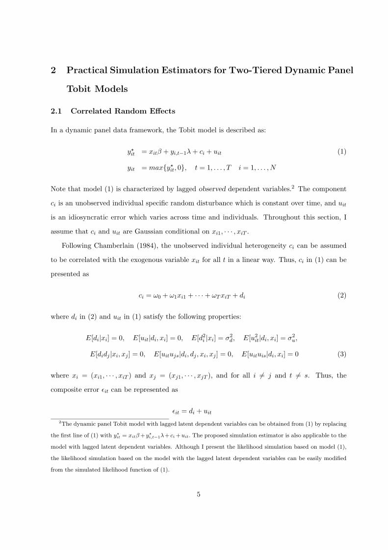
In a dynamic panel data framework, the Tobit model is described as:

y⋆it = xitβ + yi,t−1λ+ ci + uit (1)

yit = maxy⋆it, 0, t = 1, . . . , T i = 1, . . . , N

Note that model (1) is characterized by lagged observed dependent variables.2 The component

ci is an unobserved individual specific random disturbance which is constant over time, and uit

is an idiosyncratic error which varies across time and individuals. Throughout this section, I

assume that ci and uit are Gaussian conditional on xi1, · · · , xiT .

Following Chamberlain (1984), the unobserved individual heterogeneity ci can be assumed

to be correlated with the exogenous variable xit for all t in a linear way. Thus, ci in (1) can be

presented as

ci = ω0 + ω1xi1 + · · ·+ ωTxiT + di (2)

where di in (2) and uit in (1) satisfy the following properties:

E[di|xi] = 0, E[uit|di, xi] = 0, E[d2i |xi] = σ2d, E[u2it|di, xi] = σ2

u,

E[didj |xi, xj ] = 0, E[uitujs|di, dj , xi, xj ] = 0, E[uituis|di, xi] = 0 (3)

where xi = (xi1, · · · , xiT ) and xj = (xj1, · · · , xjT ), and for all i = j and t = s. Thus, the

composite error ϵit can be represented as

ϵit = di + uit

2The dynamic panel Tobit model with lagged latent dependent variables can be obtained from (1) by replacing

the first line of (1) with y⋆it = xitβ+y⋆

i,t−1λ+ ci+uit. The proposed simulation estimator is also applicable to the

model with lagged latent dependent variables. Although I present the likelihood simulation based on model (1),

the likelihood simulation based on the model with the lagged latent dependent variables can be easily modified

from the simulated likelihood function of (1).

5

Under such a specification, ω0 cannot be identified if a constant is included in xit. One

way to include a constant term in xit is to assume the independence of time constant xit and

the unobserved individual heterogeneity ci. Under such a circumstance, the coefficient of the

constant term xit can be consistently estimated using the simulation estimator. Moreover, time

dummies are also excluded from xit in ci because they do not vary across i.

For a correlated random effects approach of the Chamberlain type, however, the dimension

of the parameters to be estimated will increase at the rate T . When the time period T or the

dimension of x is small, computation is not an issue for estimating ω0, ω1, . . ., ωT , β and λ.

Otherwise, following Mundlak (1978), Hajivassiliou (1985, 1987) and Wooldridge (2002), ci can

be assumed to be as follows:

ci = ω0 + ωxi + di, xi =1

T

T∑t=1

xit (4)

and ω0 and ω can also be consistently estimated using the proposed simulation estimators.3

One advantage of using the correlated random effects approach of (4) is that, no matter

how large the time period T is, the number of parameters to be estimated will only be affected

by the dimension of xi. For a panel data set with a large T , this specification method for

unobserved individual heterogeneity will not only allow for correlation between ci and xi, but

will also make computation easier for parameter estimation. Equation (4) will be employed to

model unobserved individual heterogeneity in the empirical section.

2.2 Simulation Estimation

For the random effects plus AR(1) specification, the error term ϵit can be specified as

ϵit = di + vit

vit = ζvi,t−1 + uit. (5)

where di is defined either by (2) or (4), and uit and di continue to satisfy all of the conditions

in (3). The covariance structure of the random effects plus AR(1) specification is denoted as

ΣRE+AR(1). Moreover, the stationarity assumption |ζ| < 1 is also assumed to be satisfied for

the random effects plus AR(1) errors model.

3The time dummies and time constant variables are also not included in xi.

6

Let Iit be a censored indicator function, such that

Iit =

1 for y⋆it > 0

0 for y⋆it ≤ 0

Therefore, for individual i, if Iit = 1 then y⋆it is observed and yit = y⋆it. On the other hand, y⋆it

is censored and its value is not observed (i.e., yit = 0) if Iit = 0.

Thus, the simulated likelihood function with R simulation draws based on the GHK simulator

for individual i can be described as:

Li =1

R

R∑r=1

T∏t=1

[f (r)(yit|yi,t−1)]Iit [P (r)(Iit = 0|yi,t−1)]

1−Iit (6)

By letting li = ln(Li), the simulated log-likelihood function can be represented as:

lR = ln(N∏i=1

Li) =N∑i=1

li (7)

The error terms ϵi are assumed to have a normal distribution, that is, ϵi ∼ N(0,ΣRE+AR(1)),

where ϵi = (ϵi1, . . . , ϵiT )′ is a T × 1 column vector, and so E[ϵiϵ

′i|xi1, · · · , xiT ] = ΣRE+AR(1).

Under this assumption, the simulation estimator based on the GHK simulator is expected to be

useful for the dynamic panel Tobit models since it is well recognized that the GHK simulator

is very accurate for the simulation of a multivariate normal distribution (Hajivassiliou et al.,

1996).

Let A be the Cholesky decomposition of ΣRE+AR(1), that is, ΣRE+AR(1) = AA′, where A

is a lower-triangular matrix. Given this structure, we can write ϵi = Aηi, where ϵi = di + uit,

ηi ∼ N(0, I) and ηi = (ηi1, . . . , ηiT )′.

Let θ be the vector of parameters of interest in the random effects plus AR(1) model, i.e.,

θ = (β, λ, σ2u, σ

2d, ζ). Given the sample, suppose that for individual i the total number of instances

of censoring is mi and that censoring occurs at time t1, . . . , tmi . The random variables ξ(r)it are

drawn from the uniform random number generator on [0,1], where t = t1, . . . , tmi , i = 1, . . . , N

and r = 1, . . . R. In order to guarantee the validity of the stochastic equicontinuity condition4

for the simulation estimator, the random numbers are drawn once and kept fixed when θ varies.5

4See Hajivassiliou and McFadden (1998).5See McFadden (1989) for further details.

7

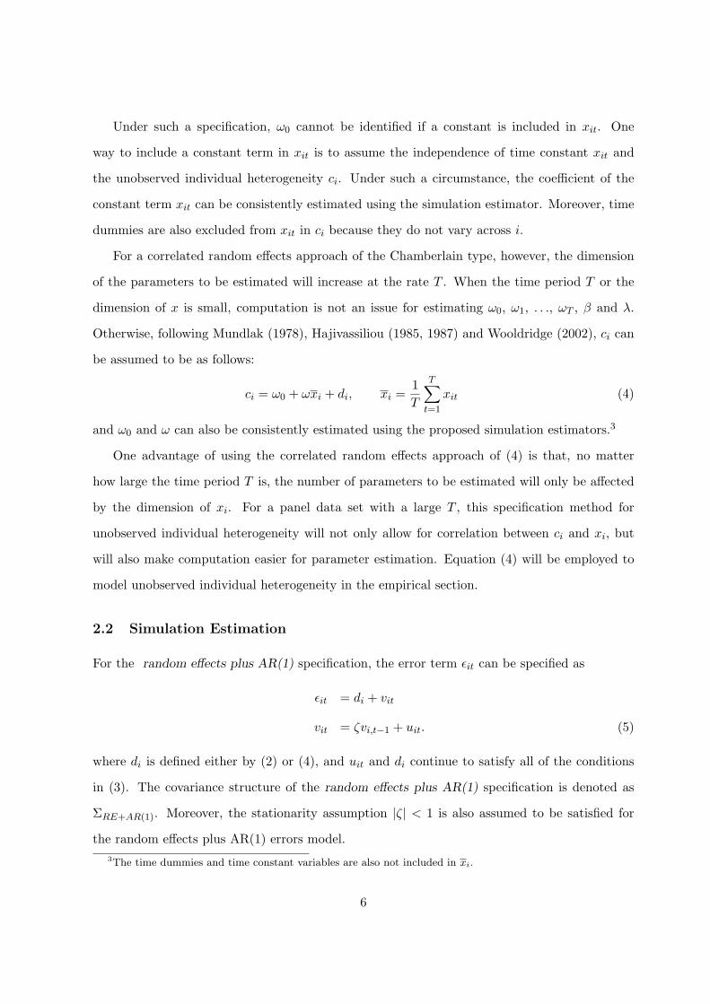
To simplify the exposition, y⋆i0 = 0 is assumed for all i. Let Φ be the cumulative stan-

dard normal function. Then, the truncated normal random variables η(r)it can be simulated or

calculated by

η(r)it =

Φ−1(ξ(r)it Φ(

−xitβ−yi,t−1λ−xiω−∑t−1

k=1Atkη

(r)ik

Att)) for t ∈ t1, . . . , tmi

yit−xitβ−yi,t−1λ−xiω−∑t−1

k=1Atkη

(r)ik

Attfor t ∈ t1, . . . , tmi

(8)

Then, the simulated likelihood function (6) can be obtained through

f (r)(yit|yi,t−1) =1

Attϕ(

yit − xitβ − yi,t−1λ− xiω −∑t−1

k=1Atkη(r)ik

Att) (9)

for t ∈ t1, . . . , tmi, where ϕ is the standard normal density function, and

P (r)(Iit = 0|yi,t−1) = Φ(−xitβ − yi,t−1λ− xiω −

∑t−1k=1Atkη

(r)ik

Att) (10)

for t ∈ t1, . . . , tmi. Thus, by combining (9) and (10) into (6), a practical simulation estimator

of θ denoted as θ can be obtained for maximizing the simulated log-likelihood function (7).

Based on the GHK simulation estimators presented above, the asymptotic variance associated

with them can be consistently estimated as follows. Let

Ω =1

NΣNi=1[si(θ)si(θ)

′]

and

J =1

NΣNi=1siθ(θ)

where si is the simulated score function associated with (7), and siθ is the first derivative of si

with respect to θ, that is, J is simply the Hessian matrix of the simulated log-likelihood function

(7). Therefore, the consistent estimator of the asymptotic variance of the simulation estimator

θ can be written as

Avar(θ) = J−1ΩJ−1. (11)

See Hajivassiliou and McFadden (1998) for more details.

The average partial effects (APEs) can also be estimated by using the GHK simulation esti-

mators θ under the correlated random effects approach. For the APEs of the decision probability

8

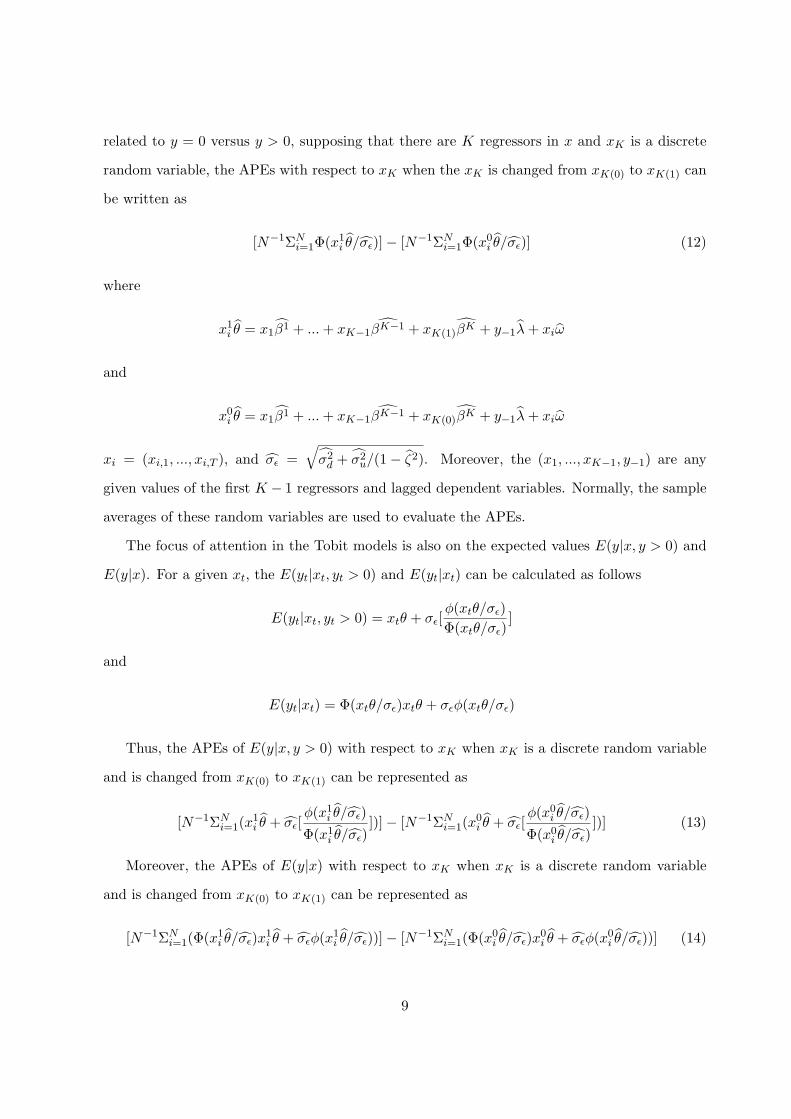
related to y = 0 versus y > 0, supposing that there are K regressors in x and xK is a discrete

random variable, the APEs with respect to xK when the xK is changed from xK(0) to xK(1) can

be written as

[N−1ΣNi=1Φ(x

1i θ/σϵ)]− [N−1ΣN

i=1Φ(x0i θ/σϵ)] (12)

where

x1i θ = x1β1 + ...+ xK−1βK−1 + xK(1)βK + y−1λ+ xiω

and

x0i θ = x1β1 + ...+ xK−1βK−1 + xK(0)βK + y−1λ+ xiω

xi = (xi,1, ..., xi,T ), and σϵ =√σ2d + σ2

u/(1− ζ2). Moreover, the (x1, ..., xK−1, y−1) are any

given values of the first K − 1 regressors and lagged dependent variables. Normally, the sample

averages of these random variables are used to evaluate the APEs.

The focus of attention in the Tobit models is also on the expected values E(y|x, y > 0) and

E(y|x). For a given xt, the E(yt|xt, yt > 0) and E(yt|xt) can be calculated as follows

E(yt|xt, yt > 0) = xtθ + σϵ[ϕ(xtθ/σϵ)

Φ(xtθ/σϵ)]

and

E(yt|xt) = Φ(xtθ/σϵ)xtθ + σϵϕ(xtθ/σϵ)

Thus, the APEs of E(y|x, y > 0) with respect to xK when xK is a discrete random variable

and is changed from xK(0) to xK(1) can be represented as

[N−1ΣNi=1(x

1i θ + σϵ[

ϕ(x1i θ/σϵ)

Φ(x1i θ/σϵ)])]− [N−1ΣN

i=1(x0i θ + σϵ[

ϕ(x0i θ/σϵ)

Φ(x0i θ/σϵ)])] (13)

Moreover, the APEs of E(y|x) with respect to xK when xK is a discrete random variable

and is changed from xK(0) to xK(1) can be represented as

[N−1ΣNi=1(Φ(x

1i θ/σϵ)x

1i θ + σϵϕ(x

1i θ/σϵ))]− [N−1ΣN

i=1(Φ(x0i θ/σϵ)x

0i θ + σϵϕ(x

0i θ/σϵ))] (14)

9

2.3 Two-tiered Dynamic Panel Tobit Models

One potential restriction of Tobit models is that of the choice between y = 0 versus y > 0 and

the decision regarding the amount of y given that y > 0 is determined by a single mechanism. In

other words, the decision related to y = 0 versus y > 0 is inseparable from the decision regarding

how much y is given that y > 0 in the traditional Tobit model. However, the mechanisms which

determine these two may not be the same in some economic models.

Specifically, any variable which increases the probability of a nonzero value must also increase

the mean of the positive values in the traditional Tobit models. This is not always the case. For

example, as for the application of the married women’s labor supply which is further discussed

in the empirical section that appears later, the traditional Tobit model indicates that married

women who have one more child aged between 6 and 13 years old should always decrease (or

increase) both the probability of labor force participation and the mean hours worked. However,

by using the more generalized types of Tobit model, it is found that married women with one

more child aged between 6 and 13 years old will increase their labor force participation rate but

will decrease the mean hours worked that are conditional on the participation.

In order to relax the restrictions imposed by the traditional Tobit models, Cragg (1971)

proposed a two-tiered model to allow the parameters which characterize the decision regarding

y = 0 versus y > 0 to be separate from the parameters which determine the decision regarding

how much y is given that y > 0. The traditional Tobit models can be viewed as a special case

of Cragg’s two-tiered model.6 In other words, there are basically two assumptions in Cragg’s

two-tiered model. First, the probability of a zero observation is given by a probit model with the

first tier parameters, and then the density of the dependent variable that is conditional on being

a positive observation is truncated at zero and characterized by the second tier parameters.

Cragg’s model is easily extended from the cross-sectional framework to the dynamic panel data

models using the simulation estimators proposed earlier.

There are alternatives to Cragg’s two-tiered models. One of the examples is the Heckman

6See for example Lin and Schmidt (1984) for a specification test of the Tobit model against Cragg’s model.

10

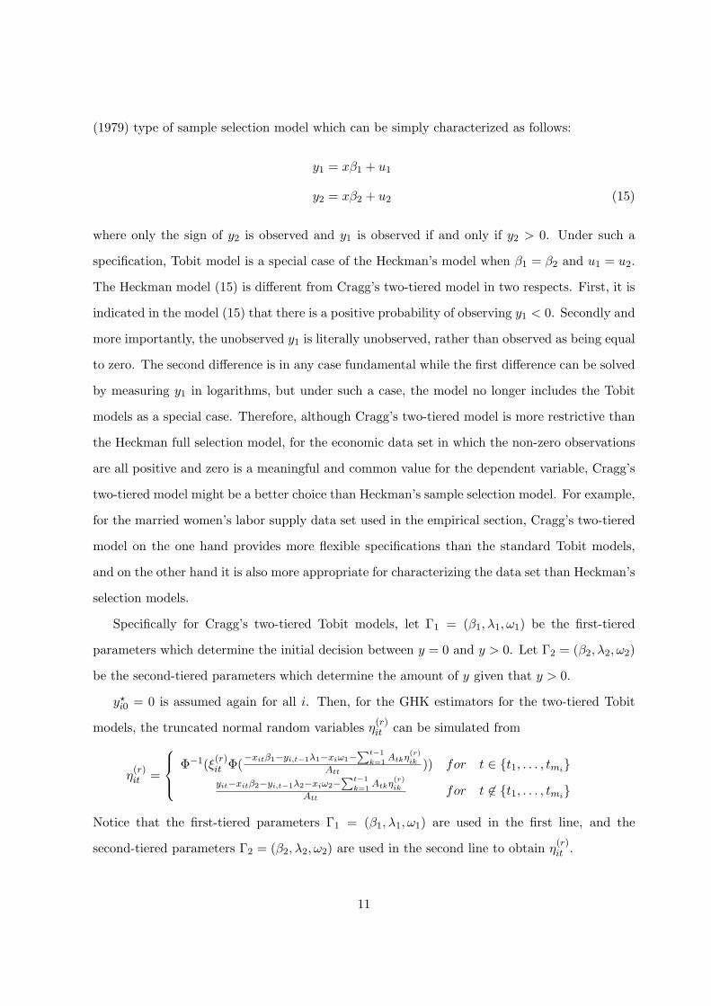
(1979) type of sample selection model which can be simply characterized as follows:

y1 = xβ1 + u1

y2 = xβ2 + u2 (15)

where only the sign of y2 is observed and y1 is observed if and only if y2 > 0. Under such a

specification, Tobit model is a special case of the Heckman’s model when β1 = β2 and u1 = u2.

The Heckman model (15) is different from Cragg’s two-tiered model in two respects. First, it is

indicated in the model (15) that there is a positive probability of observing y1 < 0. Secondly and

more importantly, the unobserved y1 is literally unobserved, rather than observed as being equal

to zero. The second difference is in any case fundamental while the first difference can be solved

by measuring y1 in logarithms, but under such a case, the model no longer includes the Tobit

models as a special case. Therefore, although Cragg’s two-tiered model is more restrictive than

the Heckman full selection model, for the economic data set in which the non-zero observations

are all positive and zero is a meaningful and common value for the dependent variable, Cragg’s

two-tiered model might be a better choice than Heckman’s sample selection model. For example,

for the married women’s labor supply data set used in the empirical section, Cragg’s two-tiered

model on the one hand provides more flexible specifications than the standard Tobit models,

and on the other hand it is also more appropriate for characterizing the data set than Heckman’s

selection models.

Specifically for Cragg’s two-tiered Tobit models, let Γ1 = (β1, λ1, ω1) be the first-tiered

parameters which determine the initial decision between y = 0 and y > 0. Let Γ2 = (β2, λ2, ω2)

be the second-tiered parameters which determine the amount of y given that y > 0.

y⋆i0 = 0 is assumed again for all i. Then, for the GHK estimators for the two-tiered Tobit

models, the truncated normal random variables η(r)it can be simulated from

η(r)it =

Φ−1(ξ(r)it Φ(

−xitβ1−yi,t−1λ1−xiω1−∑t−1

k=1Atkη

(r)ik

Att)) for t ∈ t1, . . . , tmi

yit−xitβ2−yi,t−1λ2−xiω2−∑t−1

k=1Atkη

(r)ik

Attfor t ∈ t1, . . . , tmi

Notice that the first-tiered parameters Γ1 = (β1, λ1, ω1) are used in the first line, and the

second-tiered parameters Γ2 = (β2, λ2, ω2) are used in the second line to obtain η(r)it .

11

Then the simulated likelihood function of the two-tiered version of (6) for individual i can

be described as:

Li =1

R

R∑r=1

T∏t=1

[P (Iit = 1|Γ1, yi,t−1)

P (Iit = 1|Γ2, yi,t−1)f(yit|Γ2, yi,t−1)]

Iit [P (Iit = 0|Γ1, yi,t−1)]1−Iit (16)

where the traditional Tobit models can be viewed as a special case of (16) when Γ1 = Γ2.

Specifically, f(yit|Γ2, yi,t−1), P (Iit = 1|Γ1, yi,t−1), P (Iit = 0|Γ1, yi,t−1) and P (Iit = 1|Γ2, yi,t−1)

in (16) can be calculated by

f(yit|Γ2, yi,t−1) =1

Attϕ(

yit − xitβ2 − yi,t−1λ2 − xiω2 −∑t−1

k=1Atkη(r)ik

Att) (17)

and

P (Iit = 1|Γ1, yi,t−1) = 1− Φ(−xitβ1 − yi,t−1λ1 − xiω1 −

∑t−1k=1Atkη

(r)ik

Att) (18)

and

P (Iit = 1|Γ2, yi,t−1) = 1− Φ(−xitβ2 − yi,t−1λ2 − xiω2 −

∑t−1k=1Atkη

(r)ik

Att) (19)

and P (Iit = 0|Γ1, yi,t−1) = 1− P (Iit = 1|Γ1, yi,t−1). Thus, a practical simulation estimator of θ

can be obtained for maximizing the simulated log-likelihood function by using (16). Moreover,

the consistent estimator of the asymptotic variance of the two-tiered simulation estimators can

be obtained through (11). The two-tiered dynamic panel Tobit model will be applied to study

the married women’s labor supply in the empirical section.

The APEs of two-tiered Tobit models can also be estimated by using the GHK simulation es-

timators. Let θ1 = (β(1), λ(1), ω(1)) be the estimators from the first tier, and θ2 = (β(2), λ(2), ω(2))

be the estimators from the second tier. Then the APEs of the decision probability are related

to y = 0 versus y > 0, supposing again that there are K regressors in x and xK is a discrete

random variable. The APEs with respect to xK when xK is changed from xK(0) to xK(1) can

be written as

[N−1ΣNi=1Φ(x

1θ(1)/σϵ)]− [N−1ΣNi=1Φ(x

0θ(1)/σϵ)] (20)

where it is assumed that

x1θ(1) = x1β1(1) + ...+ xK−1

βK−1(1) + xK(1)β

K(1) + y−1λ(1) + xiω(1)

12

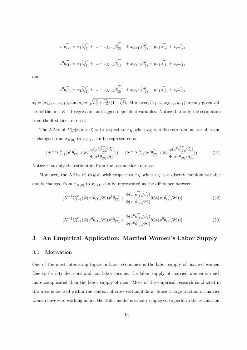
x1θ(2) = x1β1(2) + ...+ xK−1

βK−1(2) + xK(1)β

K(2) + y−1λ(2) + xiω(2)

x0θ(1) = x1β1(1) + ...+ xK−1

βK−1(1) + xK(0)β

K(1) + y−1λ(1) + xiω(1)

and

x0θ(2) = x1β1(2) + ...+ xK−1

βK−1(2) + xK(0)β

K(2) + y−1λ(2) + xiω(2)

xi = (xi,1, ..., xi,T ), and σϵ =√σ2d + σ2

u/(1− ζ2). Moreover, (x1, ..., xK−1, y−1) are any given val-

ues of the first K−1 regressors and lagged dependent variables. Notice that only the estimators

from the first tier are used.

The APEs of E(y|x, y > 0) with respect to xK when xK is a discrete random variable and

is changed from xK(0) to xK(1) can be represented as

[N−1ΣNi=1(x

1θ(2) + σϵ[ϕ(x1θ(2)/σϵ)

Φ(x1θ(2)/σϵ)])]− [N−1ΣN

i=1(x0θ(2) + σϵ[

ϕ(x0θ(2)/σϵ)

Φ(x0θ(2)/σϵ)])] (21)

Notice that only the estimators from the second tier are used.

Moreover, the APEs of E(y|x) with respect to xK when xK is a discrete random variable

and is changed from xK(0) to xK(1) can be represented as the difference between

[N−1ΣNi=1(Φ(x

1θ(1)/σϵ)x1θ(2) +

Φ(x1θ(1)/σϵ)

Φ(x1θ(2)/σϵ)σϵϕ(x

1θ(2)/σϵ))] (22)

[N−1ΣNi=1(Φ(x

0θ(1)/σϵ)x0θ(2) +

Φ(x0θ(1)/σϵ)

Φ(x0θ(2)/σϵ)σϵϕ(x

0θ(2)/σϵ))] (23)

3 An Empirical Application: Married Women’s Labor Supply

3.1 Motivation

One of the most interesting topics in labor economics is the labor supply of married women.

Due to fertility decisions and non-labor income, the labor supply of married women is much

more complicated than the labor supply of men. Most of the empirical research conducted in

this area is focused within the context of cross-sectional data. Since a large fraction of married

women have zero working hours, the Tobit model is usually employed to perform the estimation.

13

Jakubson (1988) incorporated the life-cycle model into the married women’s labor supply

equation and estimated the model using four-year panel data. Hyslop (1999) also applied the

panel Probit model with a rich dynamic structure to study the labor force participation of

married women. It is crucial to incorporate the dynamic structure into the married women’s

labor supply function as indicated in Hyslop’s results. Moreover, in analyzing the interactions

between fertility and the labor supply decision for married women, Browning (1992) pointed out

that it is important to control for the dynamic structure of their labor supply decisions.

In a dynamic structure, it is often argued that individuals who have experienced an event

in the past are more likely to experience the same event in the future than individuals who did

not experience the event. This is what Heckman (1981) refers to as “state dependence.” There

are two types of state dependence in a dynamic structure. One is “true state dependence,”

and the other is “spurious state dependence.” True state dependence, as explained by Heckman

(1981), is when “as a consequence of experiencing an event, preference, prices or constraints

relevant to future choice are altered.” On the other hand, Heckman (1981) explains spurious state

dependence as “the phenomenon that individuals may differ in their propensity to experience

the event. If individual differences are correlated over time, and if these differences are not

properly controlled, previous experience may appear to be a determinant of future experience.”

Therefore, it is important for economists to distinguish true state dependence from spurious

state dependence in the labor supply function of married women.

The empirical specification for modeling the labor supply of married women in this section

involves the reduced form method. There is also a huge literature on structural models of female

labor supply, for example, Heckman and MaCurdy (1980, 1982) and Eckstein and Wolpin (1989).

Although the reduced form methods are useful for initial exploratory data analysis and they are

relatively easy to implement compared with the structural form methods, there are several

advantages in structural estimation. The first advantage of having a structural model behind

the estimations is that the parameters estimated can be interpreted in a way that is consistent

with the theoretical framework. In other words, the detailed implications of the theory, and

not only of the data, can be learned during the process of estimating the structural models.

Moreover, the predictions of the impacts of policy changes can be generated more accurately

14

by the structural models than by the reduced form models. See Rust (1994) for more details

regarding the structural estimation.

In this section, the two-tiered dynamic panel Tobit model is employed to study the labor

supply of married women. Unlike the models estimated by Cogan (1981) and Mroz (1987),

panel data are used in the estimation. In addition, rather than using the static panel Tobit

model estimated by Jakubson (1988), rich dynamic structures are incorporated in the model and

estimated by the proposed simulation estimators. Moreover, decisions over both participation

and hours are considered through the Tobit structure, while Hyslop (1999) only focuses on the

labor force participation decision for married women. Since Cogan (1981) and Mroz (1987) have

pointed out a possible mis-specification of the simple Tobit specification for the labor supply

of married women due to the significant fixed cost involved in their labor force participation

decisions, the Cragg type two-tiered Tobit model is also implemented to study the labor supply

of married women.

3.2 Data

The data used in the estimation consist of a nine-year panel data set from the PSID. The sample

contains observations for 1,627 women continuously married between 1984 and 1992, and aged

between 19 and 60 in 1985. Table 1 presents the summary statistics for the data used. The

husband’s income in Table 1 is expressed in constant (1985) thousands of dollars, computed as

nominal earnings deflated by the consumer price index. The numbers in the parentheses are the

standard errors corresponding to the variables.

The distribution of years worked during the period for the full sample in Table 1 also suggests

the importance of incorporating the dynamic structure for the married women’s labor supply.

For example, supposing that the individual’s participation decision is distributed according to

an independent binomial distribution, then about 9.08% of the sample would be expected to

work each year if the participation probability were fixed as 0.766 (the average participation

rate during the period), about 13.42% of the sample would be expected to work each year if the

participation probability were fixed as 0.8, and about 4.04% of the sample would be expected

to work each year if the participation probability were fixed as 0.7. In these three cases, less

15

Table 1. Sample Characteristics

Variable Full Employed Employed Employed

Name Sample 9 Years 0 Years ≥ 1 Year

Age (1985) 34.68(8.769)

34.77(8.144)

41.99(9.520)

34.22(8.723)

Education 12.89(2.071)

13.14(2.031)

12.07(1.987)

12.94(2.077)

Race (Black=1) 0.212(0.409)

0.233(0.423)

0.240(0.427)

0.210(0.408)

Husband’s Income ($1000) 31.04(29.16)

28.99(24.59)

40.51(42.81)

30.45(28.10)

Children between 1 and 2 0.218(0.466)

0.173(0.419)

0.176(0.456)

0.221(0.467)

Children between 3 and 5 0.277(0.516)

0.222(0.462)

0.242(0.523)

0.279(0.516)

Children between 6 and 13 0.712(0.891)

0.659(0.849)

0.616(0.844)

0.718(0.894)

Hours of Work 1179.88(887.01)

1695.84(593.45)

0 1253.86(914.41)

No. of years worked

zero 96 − 96 −

one 50 − − 50

two 56 − − 56

three 65 − − 65

four 66 − − 66

five 77 − − 77

six 83 − − 83

seven 115 − − 115

eight 149 − − 149

nine 870 870 − 870

Sample Size 1627 870 96 1531

16

than 0.002% of the sample would be expected not to work at all. However, the sample’s relative

frequencies are 53.47% of the sample who worked each year for 9 years and 5.9% of the sample

who did not work at all, accordingly. Therefore, Table 1 indicates that there is significant

persistence in the observed annual participation decisions of married women.

The differences in the characteristics of the married women across the sub-samples shown

in Table 1 can be interpreted as follows. Women who work each year are better educated, are

more likely to be black, have lower than average husband’s income, and have fewer dependent

children. On the other hand, women who have never been employed during the sample period

are older, less educated, are more likely to be black, have higher than average husband’s income,

and have slightly fewer dependent children.

3.3 Estimation Results

The dynamic panel Tobit model (1) with the covariance matrix ΣRE+AR(1) under the assump-

tions in (3) is employed to study the labor supply of married women. The dependent variable

is the annual hours of work. The explanatory variables include constants (Cons), years of

schooling (Edu), wife’s race (Race, black=1), wife’s age (Age), square of age (Age2), husband’s

income (Hinc), number of children aged between 1 and 2 years old (C12), number of children

aged between 3 and 5 years old (C35), and number of children aged between 6 and 13 years

old (C613). The husband’s income is used as a proxy variable for non-labor income for married

women. Furthermore, the lagged dependent variable is not included as a regressor in the static

models. The numbers in the parentheses are the estimated standard errors corresponding to

the estimators. The optimization subroutine used is the ConstrOptim procedure based on the

R software, and the BFGS algorithm is used for the maximization.7

The estimation results are presented in Table 2 for the static models. The pure random

effects plus AR(1) model which assumes that ci = di is presented as model (1) of Table 2. It is

shown that better educated or black or older women tend to work more than less educated or

white or younger women. In addition, the women who have children, especially children between

the ages of 1 and 2, tend to work less than the women who have no children. These results are

7The same procedure and algorithm are used later in the Monte Carlo experiments subsection.

17

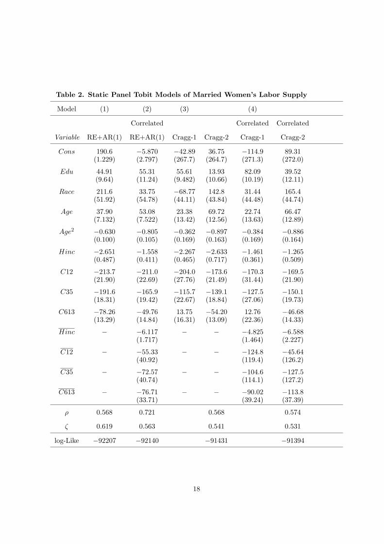
Table 2. Static Panel Tobit Models of Married Women’s Labor Supply

Model (1) (2) (3) (4)

Correlated Correlated Correlated

Variable RE+AR(1) RE+AR(1) Cragg-1 Cragg-2 Cragg-1 Cragg-2

Cons 190.6(1.229)

−5.870(2.797)

−42.89(267.7)

36.75(264.7)

−114.9(271.3)

89.31(272.0)

Edu 44.91(9.64)

55.31(11.24)

55.61(9.482)

13.93(10.66)

82.09(10.19)

39.52(12.11)

Race 211.6(51.92)

33.75(54.78)

−68.77(44.11)

142.8(43.84)

31.44(44.48)

165.4(44.74)

Age 37.90(7.132)

53.08(7.522)

23.38(13.42)

69.72(12.56)

22.74(13.63)

66.47(12.89)

Age2 −0.630(0.100)

−0.805(0.105)

−0.362(0.169)

−0.897(0.163)

−0.384(0.169)

−0.886(0.164)

Hinc −2.651(0.487)

−1.558(0.411)

−2.267(0.465)

−2.633(0.717)

−1.461(0.361)

−1.265(0.509)

C12 −213.7(21.90)

−211.0(22.69)

−204.0(27.76)

−173.6(21.49)

−170.3(31.44)

−169.5(21.90)

C35 −191.6(18.31)

−165.9(19.42)

−115.7(22.67)

−139.1(18.84)

−127.5(27.06)

−150.1(19.73)

C613 −78.26(13.29)

−49.76(14.84)

13.75(16.31)

−54.20(13.09)

12.76(22.36)

−46.68(14.33)

Hinc − −6.117(1.717)

− − −4.825(1.464)

−6.588(2.227)

C12 − −55.33(40.92)

− − −124.8(119.4)

−45.64(126.2)

C35 − −72.57(40.74)

− − −104.6(114.1)

−127.5(127.2)

C613 − −76.71(33.71)

− − −90.02(39.24)

−113.8(37.39)

ρ 0.568 0.721 0.568 0.574

ζ 0.619 0.563 0.541 0.531

log-Like −92207 −92140 −91431 −91394

18

standard in the literature. The fraction of the variance due to individual heterogeneity, ρ, is

0.568, and the AR(1) coefficient ζ is 0.619.

The unobserved individual heterogeneity ci in the correlated random effects plus AR(1)

model (2) of Table 2 is assumed to be as follows:

ci = ω0 + ω1Hinci + ω2C12i + ω3C35i + ω4C613i + di (24)

where Hinci, C12i, C35i, C613i are time averages of the corresponding variables for individual

i. Based on model (2) of Table 2, it is shown later in Table 4 that both the husband’s income

and fertility decision variables are endogenous in the static model (1) of Table 2 at the 1%

significance level. Thus, the impact of education and age is underestimated and the impact of

race and younger children is overestimated in model (1) of Table 2 if the endogeneity problem

is ignored. Moreover, ρ increases and the AR(1) coefficient ζ decreases from model (2) to model

(1) in Table 2.

The two-tiered Cragg type panel Tobit model is estimated in model (3) of Table 2 where the

decisions on labor force participation and hours worked that are conditional on the participation

are estimated separately. Based on model (3) of Table 2, the women receiving higher education

are more likely to participate in the labor force. However, being conditional on the participation,

education has no statistically significant impact on the decision regarding hours worked. On the

other hand, in a way that is conditional on participation in the labor force, black or older women

tend to work more than white or younger women, but there is no statistically significant impact

of race or age on the labor force participation decision for married women. The husband’s income

has almost the same negative impact on both the participation and working hours decisions.

Thus, for married women, the higher the husband’s income, the less likely it is that she will

participate in the labor force, and the less hours she will work if she decides to participate in the

labor force. The children aged between 1 and 5 years old have a negative impact on the married

women in both the participation as well as hours worked decisions, and not surprisingly, the

younger the children, the stronger the negative impact will be on both margins. The children

aged between 6 and 13 years old also have a negative impact on the working hours decision that

is conditional on the participation. However, they may have a positive impact on the labor force

19

participation decision although this positive influence is not statistically significant. The ρ and

AR(1) coefficient ζ in model (3) are similar to the ones in model (1) of Table 2.

The static correlated Cragg’s two-tiered model is estimated in model (4) of Table 2 by

using (24). The husband’s income is still endogenous in both tiers of the model. However, the

coefficients of C12i and C35i are each insignificant at the 10% level. Moreover, unlike model

(3) of Table 2, education has a statistically significant positive impact on both the participation

and working hours decisions.

The dynamic panel Tobit model is employed to study the labor supply for married women

in Table 3. The initial conditions problem is dealt with in Heckman’s approach. The true state

dependence parameters λ are close to zero and are not statistically significant in the RE+AR(1)

model but are marginally statistically significant in the correlated RE+AR(1) model. Moreover,

the AR(1) coefficient ζ increases slightly from Table 2 to Table 3. The correlated random effects

plus AR(1) model in (2) of Table 3 is based on (24). The coefficients of Hinci, C12i, C35i,

C613i are marginally statistically significantly different from zero at the 5% significance level

which indicates that the husband’s income as well as fertility decisions are endogenous in the

dynamic model.

The two-tiered Cragg’s type dynamic panel Tobit model is estimated in model (3) of Table 3.

As in Table 2, it can be shown that education only has a statistically significant impact on the

labor force participation decision, but not on the hours worked decision that is conditional on the

participation. On the other hand, in a way that is conditional on the participation in the labor

force, black women tend to work more than white women. However, there is no statistically

significant impact of race on the labor force participation decision. The husband’s income also

has an equally negative impact on both participation and the hours worked decision, as shown

in Table 2. Moreover, the children between 1 and 5 years of age have a statistically significant

negative impact on both participation as well as the hours worked decision. The children aged

between 6 and 13 only have a negative impact on the working hours decision that is conditional

on the participation, but there is no statistically significant impact for the children aged between

6 and 13 on the labor force participation decision for married women.

The dynamic version of the correlated Cragg’s two-tiered model is estimated in model (4)

20

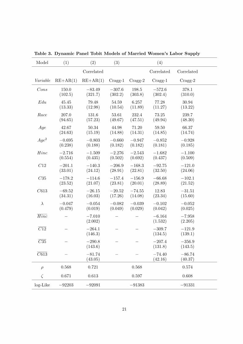
Table 3. Dynamic Panel Tobit Models of Married Women’s Labor Supply

Model (1) (2) (3) (4)

Correlated Correlated Correlated

Variable RE+AR(1) RE+AR(1) Cragg-1 Cragg-2 Cragg-1 Cragg-2

Cons 150.0(102.5)

−83.49(321.7)

−307.6(302.2)

198.5(303.8)

−572.6(302.4)

378.1(310.0)

Edu 45.45(13.33)

79.48(12.98)

54.59(10.54)

6.257(11.89)

77.28(11.27)

30.94(13.22)

Race 207.0(94.65)

131.6(57.23)

53.61(49.67)

232.4(47.51)

73.25(49.94)

239.7(48.30)

Age 42.67(24.63)

50.34(15.19)

44.98(14.88)

71.20(14.31)

59.50(14.85)

66.37(14.74)

Age2 −0.695(0.238)

−0.803(0.188)

−0.660(0.182)

−0.947(0.182)

−0.852(0.181)

−0.928(0.185)

Hinc −2.716(0.554)

−1.509(0.435)

−2.276(0.502)

−2.543(0.692)

−1.682(0.437)

−1.100(0.509)

C12 −201.1(33.01)

−140.3(24.12)

−206.9(28.91)

−168.3(22.81)

−92.75(32.50)

−121.0(24.06)

C35 −178.2(23.52)

−114.6(21.07)

−157.4(23.81)

−156.9(20.01)

−66.68(28.89)

−102.1(21.52)

C613 −69.52(34.31)

−26.15(16.03)

−20.52(17.26)

−74.55(14.08)

12.83(23.34)

−31.51(15.60)

λ −0.047(0.479)

−0.054(0.019)

−0.082(0.049)

−0.039(0.029)

−0.102(0.042)

−0.052(0.025)

Hinc − −7.010(2.002)

− − −6.164(1.532)

−7.958(2.205)

C12 − −264.1(146.3)

− − −309.7(134.5)

−121.9(139.1)

C35 − −290.8(143.6)

− − −207.4(131.8)

−356.9(143.5)

C613 − −81.74(43.05)

− − −74.40(42.16)

−86.74(40.37)

ρ 0.568 0.721 0.568 0.574

ζ 0.671 0.613 0.597 0.608

log-Like −92203 −92091 −91383 −91331

21

of Table 3. The hypothesis of the exogeneity of the husband’s income can be rejected at the

5% significance level in both the first and second tier of the estimation. The impacts of race

and age on the married women’s labor supply in model (4) of Table 3 are similar to those in

model (3) of Table 3. However, education now has a statistically significant positive impact on

both the labor force participation decision and the mean hours worked decision conditional on

the participation. Most interestingly, in the dynamic correlated Cragg’s two-tiered model it is

found that the children aged between 6 and 13 years old will give the married women a positive

incentive to participate in the labor force.

The estimators of the true state dependence parameter λ are all negative and range from

−0.102 to −0.039 in Table 3. They are statistically significant only in the correlated random

effects models. On the other hand, the estimators of the spurious state dependence parameter

ζ are slightly larger in Table 3 than in Table 2. The estimators of the ρ in Table 3 are similar

to the ones in Table 2. Thus, based on Cragg’s two-tiered models that adopt the correlated

random effects approach, there is a significant true state dependence in both the participation

and hours worked decision for the married women’s labor supply. The ignorance of the true

state dependence parameter, λ, will lead to an overestimation of the spurious state dependence

parameter, ζ, as shown in Tables 2 and 3.

In order to investigate the exogeneity of the fertility decisions and the husband’s income to

the married women’s labor supply function in various models, the Wald statistics and t statistics

of the following hypotheses are performed for the correlated random effects models in Tables 2

and 3.

The hypothesis that the fertility decisions are exogenous to the married women’s labor supply

function can be written as

H0 : ω2 = 0, ω3 = 0, ω4 = 0 (25)

where ω2, ω3 and ω4 are defined in (24). The fertility decisions are endogenous to the married

women’s labor supply function if the null hypothesis (25) is rejected. This null hypothesis can

be tested based on the Wald statistics.

Moreover, the hypothesis that the husband’s income is exogenous to the married women’s

22

labor supply function can be represented as

H0 : ω1 = 0

where ω1 is defined in (24). This null hypothesis can be tested using t statistics for the tradi-

tional Tobit model and Wald statistics for Cragg’s two-tiered model. The husband’s income is

endogenous to the married women’s labor supply function if H0 : ω1 = 0 is rejected.

The test results are reported in Table 4. At the 1% significance level, the hypothesis that

the fertility decisions are exogenous to the married women’s labor supply function is rejected

in both the dynamic and static models. Moreover, the hypothesis that the husband’s income

is exogenous to the married women’s labor supply function is also rejected in all models at the

1% significance level. Therefore, there is strong evidence that both fertility decisions and the

husband’s income may not be exogenous variables in both the static and dynamic models of the

married women’s labor supply function.

3.4 Average Partial Effects

In order to investigate the impact of the fertility decisions and the change in the husband’s

income on the married women’s participation decisions and expected hours worked, the APEs

of the fertility decisions and husband’s income changes for married women are presented using

equations (12)-(14) and equations (20)-(23). By employing both standard Tobit models and

Cragg’s two-tiered models, the following four events are considered: 1. having a child aged less

than 2 years old, 2. having a child aged between 3 and 5 years old, 3. having a child aged

between 6 and 13 years old, and 4. 10% increases in the husband’s income. Two types of APEs

of expected hours worked for married women are considered, that is, one unconditional and

another conditional on the labor force participation. It is assumed that a married woman has

no children in the base model. The age and husband’s income of the married woman are set

equal to the sample average, that is Age = 38 and Hinc = 31, 000. Moreover, two education

levels are considered for estimating the average partial effects, one being Edu = 12 (possibly

high school graduates), and the other Edu = 16 (possibly college graduates).

Three types of APEs are reported in Tables 5-7. P.P. stands for the labor force participation

23

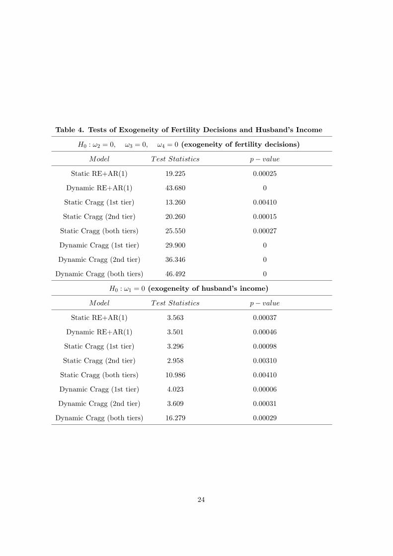
Table 4. Tests of Exogeneity of Fertility Decisions and Husband’s Income

H0 : ω2 = 0, ω3 = 0, ω4 = 0 (exogeneity of fertility decisions)

Model Test Statistics p− value

Static RE+AR(1) 19.225 0.00025

Dynamic RE+AR(1) 43.680 0

Static Cragg (1st tier) 13.260 0.00410

Static Cragg (2nd tier) 20.260 0.00015

Static Cragg (both tiers) 25.550 0.00027

Dynamic Cragg (1st tier) 29.900 0

Dynamic Cragg (2nd tier) 36.346 0

Dynamic Cragg (both tiers) 46.492 0

H0 : ω1 = 0 (exogeneity of husband’s income)

Model Test Statistics p− value

Static RE+AR(1) 3.563 0.00037

Dynamic RE+AR(1) 3.501 0.00046

Static Cragg (1st tier) 3.296 0.00098

Static Cragg (2nd tier) 2.958 0.00310

Static Cragg (both tiers) 10.986 0.00410

Dynamic Cragg (1st tier) 4.023 0.00006

Dynamic Cragg (2nd tier) 3.609 0.00031

Dynamic Cragg (both tiers) 16.279 0.00029

24

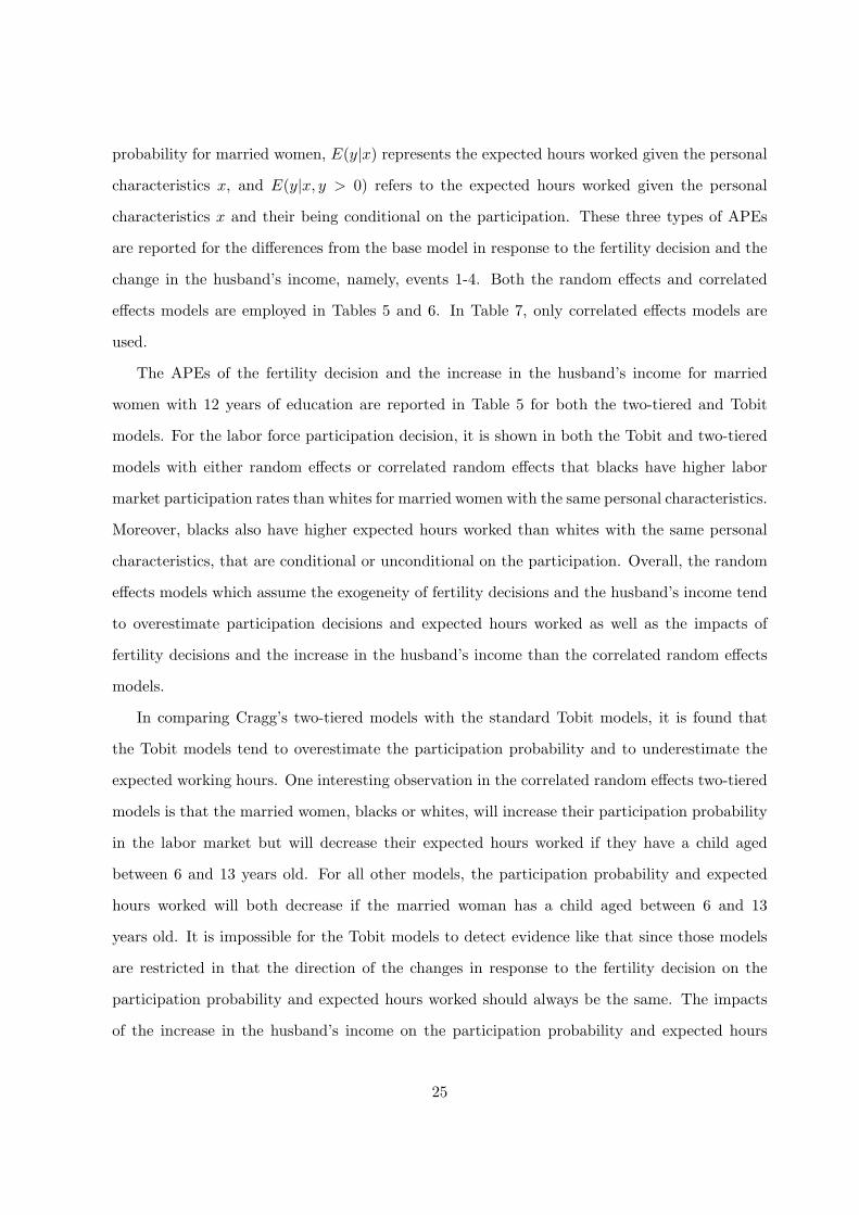
probability for married women, E(y|x) represents the expected hours worked given the personal

characteristics x, and E(y|x, y > 0) refers to the expected hours worked given the personal

characteristics x and their being conditional on the participation. These three types of APEs

are reported for the differences from the base model in response to the fertility decision and the

change in the husband’s income, namely, events 1-4. Both the random effects and correlated

effects models are employed in Tables 5 and 6. In Table 7, only correlated effects models are

used.

The APEs of the fertility decision and the increase in the husband’s income for married

women with 12 years of education are reported in Table 5 for both the two-tiered and Tobit

models. For the labor force participation decision, it is shown in both the Tobit and two-tiered

models with either random effects or correlated random effects that blacks have higher labor

market participation rates than whites for married women with the same personal characteristics.

Moreover, blacks also have higher expected hours worked than whites with the same personal

characteristics, that are conditional or unconditional on the participation. Overall, the random

effects models which assume the exogeneity of fertility decisions and the husband’s income tend

to overestimate participation decisions and expected hours worked as well as the impacts of

fertility decisions and the increase in the husband’s income than the correlated random effects

models.

In comparing Cragg’s two-tiered models with the standard Tobit models, it is found that

the Tobit models tend to overestimate the participation probability and to underestimate the

expected working hours. One interesting observation in the correlated random effects two-tiered

models is that the married women, blacks or whites, will increase their participation probability

in the labor market but will decrease their expected hours worked if they have a child aged

between 6 and 13 years old. For all other models, the participation probability and expected

hours worked will both decrease if the married woman has a child aged between 6 and 13

years old. It is impossible for the Tobit models to detect evidence like that since those models

are restricted in that the direction of the changes in response to the fertility decision on the

participation probability and expected hours worked should always be the same. The impacts

of the increase in the husband’s income on the participation probability and expected hours

25

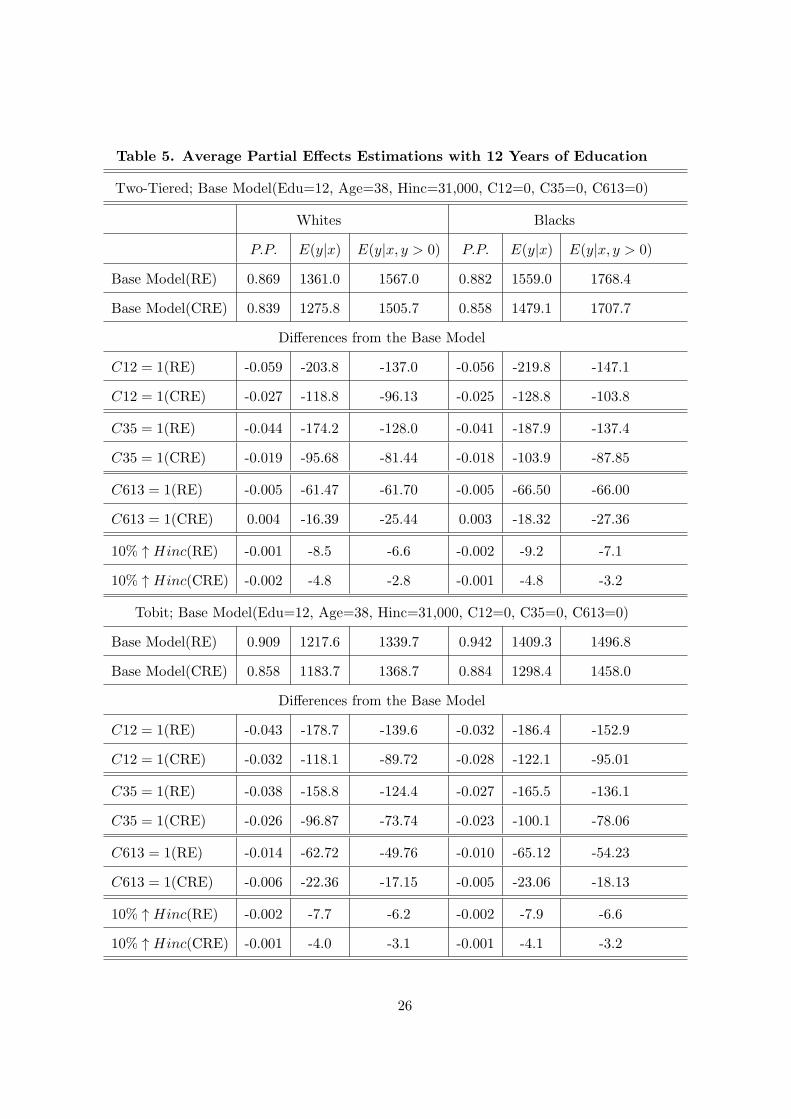
Table 5. Average Partial Effects Estimations with 12 Years of Education

Two-Tiered; Base Model(Edu=12, Age=38, Hinc=31,000, C12=0, C35=0, C613=0)

Whites Blacks

P.P. E(y|x) E(y|x, y > 0) P.P. E(y|x) E(y|x, y > 0)

Base Model(RE) 0.869 1361.0 1567.0 0.882 1559.0 1768.4

Base Model(CRE) 0.839 1275.8 1505.7 0.858 1479.1 1707.7

Differences from the Base Model

C12 = 1(RE) -0.059 -203.8 -137.0 -0.056 -219.8 -147.1

C12 = 1(CRE) -0.027 -118.8 -96.13 -0.025 -128.8 -103.8

C35 = 1(RE) -0.044 -174.2 -128.0 -0.041 -187.9 -137.4

C35 = 1(CRE) -0.019 -95.68 -81.44 -0.018 -103.9 -87.85

C613 = 1(RE) -0.005 -61.47 -61.70 -0.005 -66.50 -66.00

C613 = 1(CRE) 0.004 -16.39 -25.44 0.003 -18.32 -27.36

10% ↑ Hinc(RE) -0.001 -8.5 -6.6 -0.002 -9.2 -7.1

10% ↑ Hinc(CRE) -0.002 -4.8 -2.8 -0.001 -4.8 -3.2

Tobit; Base Model(Edu=12, Age=38, Hinc=31,000, C12=0, C35=0, C613=0)

Base Model(RE) 0.909 1217.6 1339.7 0.942 1409.3 1496.8

Base Model(CRE) 0.858 1183.7 1368.7 0.884 1298.4 1458.0

Differences from the Base Model

C12 = 1(RE) -0.043 -178.7 -139.6 -0.032 -186.4 -152.9

C12 = 1(CRE) -0.032 -118.1 -89.72 -0.028 -122.1 -95.01

C35 = 1(RE) -0.038 -158.8 -124.4 -0.027 -165.5 -136.1

C35 = 1(CRE) -0.026 -96.87 -73.74 -0.023 -100.1 -78.06

C613 = 1(RE) -0.014 -62.72 -49.76 -0.010 -65.12 -54.23

C613 = 1(CRE) -0.006 -22.36 -17.15 -0.005 -23.06 -18.13

10% ↑ Hinc(RE) -0.002 -7.7 -6.2 -0.002 -7.9 -6.6

10% ↑ Hinc(CRE) -0.001 -4.0 -3.1 -0.001 -4.1 -3.2

26

worked are relatively negligible compared with the impacts of the fertility decisions.

The APEs of the fertility decisions and the increase in the husband’s income for married

women with 16 years of education are presented in Table 6 for both the two-tiered and Tobit

models. It is reported in Table 6 that, with all other things being equal, the higher the education

level, the higher the labor force participation probability and expected hours worked that the

married women will have. Moreover, in response to the fertility decisions and the increase in

the husband’s income, the APEs have a smaller impact on labor force participation probabil-

ity for a married woman with 16 years of education than for one with 12 years of education.

Overall, the better educated married women will have higher labor force participation rates

and higher numbers of expected hours worked, whether they be conditional or unconditional on

the participation. Moreover, their participation decisions are less sensitive to the fertility deci-

sions than those of the less educated married women. In Table 6, blacks also have higher labor

market participation rates and expected hours worked than the whites in the case of married

women with the same personal characteristics. Furthermore, when compared with the correlated

random effects models, the random effects models also tend to overestimate the participation

probability, the expected hours worked and the impacts of fertility decisions and the increase in

the husband’s income. As in Table 5, the impacts of the increase in the husband’s income on

the participation probability and expected hours worked are also relatively negligible compared

with the impacts of the fertility decisions in Table 6.

In order to investigate the impacts of the fertility decisions on different age groups, the

APEs for married women between 20 and 40 years old are presented in Table 7 for two different

education levels. The participation probability and expected hours worked reported in Table 7

are for the married women with the same personal characteristics as in the base model, except

that C12 = 1, that is, with one child aged less than 2 years old. The numbers reported in

the parentheses are the APEs that are different from those in the base model. That is, these

numbers represent the impact of having one child aged less than 2 years old on the participation

probability and expected hours worked. For example, for a 20-year-old white married woman

with only one child aged less than 2 years old, a husband with an income of $31, 000, and 12 years

of education, the labor force participation rate is expected to be 0.75, the expected numbers of

27

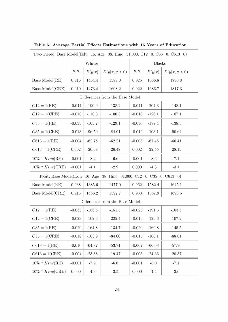
Table 6. Average Partial Effects Estimations with 16 Years of Education

Two-Tiered; Base Model(Edu=16, Age=38, Hinc=31,000, C12=0, C35=0, C613=0)

Whites Blacks

P.P. E(y|x) E(y|x, y > 0) P.P. E(y|x) E(y|x, y > 0)

Base Model(RE) 0.916 1454.4 1588.0 0.925 1656.8 1790.8

Base Model(CRE) 0.910 1473.4 1608.2 0.922 1686.7 1817.3

Differences from the Base Model

C12 = 1(RE) -0.044 -190.9 -138.2 -0.041 -204.3 -148.1

C12 = 1(CRE) -0.018 -118.3 -100.3 -0.016 -126.1 -107.1

C35 = 1(RE) -0.033 -165.7 -129.1 -0.030 -177.4 -138.3

C35 = 1(CRE) -0.013 -96.59 -84.91 -0.012 -103.1 -90.64

C613 = 1(RE) -0.004 -62.78 -62.21 -0.003 -67.45 -66.41

C613 = 1(CRE) 0.002 -20.68 -26.48 0.002 -22.55 -28.19

10% ↑ Hinc(RE) -0.001 -8.2 -6.6 -0.001 -8.6 -7.1

10% ↑ Hinc(CRE) -0.001 -4.1 -2.9 0.000 -4.3 -3.1

Tobit; Base Model(Edu=16, Age=38, Hinc=31,000, C12=0, C35=0, C613=0)

Base Model(RE) 0.938 1385.6 1477.0 0.962 1582.4 1645.1

Base Model(CRE) 0.915 1466.2 1592.7 0.933 1587.9 1693.5

Differences from the Base Model

C12 = 1(RE) -0.033 -185.6 -151.3 -0.023 -191.3 -163.5

C12 = 1(CRE) -0.023 -102.3 -225.4 -0.019 -129.6 -107.2

C35 = 1(RE) -0.029 -164.8 -134.7 -0.020 -169.8 -145.5

C35 = 1(CRE) -0.018 -103.9 -84.00 -0.015 -106.1 -88.01

C613 = 1(RE) -0.010 -64.87 -53.71 -0.007 -66.63 -57.76

C613 = 1(CRE) -0.004 -23.88 -19.47 -0.003 -24.36 -20.37

10% ↑ Hinc(RE) -0.001 -7.9 -6.6 -0.001 -8.0 -7.1

10% ↑ Hinc(CRE) 0.000 -4.3 -3.5 0.000 -4.4 -3.6

28

Table 7. Average Partial Effects Estimations with Different Age Groups

Whites Blacks

Age P.P. E(y|x) E(y|x, y > 0) P.P. E(y|x) E(y|x, y > 0)

Two-tiered CRE; Base Model(Edu=12, Hinc=31,000, C12=0, C35=0, C613=0)

20 0.750(−0.032)

945.4(−109.1)

1242.1(−87.73)

0.776(−0.030)

1116.9(−121.0)

1420.4(−96.62)

25 0.787(−0.029)

1061.3(−114.6)

1331.4(−92.43)

0.811(−0.027)

1245.3(−125.5)

1518.7(−100.7)

30 0.807(−0.028)

1135.2(−117.6)

1389.4(−95.21)

0.829(−0.025)

1326.3(−127.9)

1582.0(−103.3)

35 0.814(−0.027)

1163.1(−118.8)

1412.7(−96.28)

0.835(−0.025)

1356.8(−128.8)

1607.4(−103.9)

40 0.807(−0.028)

1143.5(−118.4)

1400.2(−95.71)

0.829(−0.025)

1335.6(−128.6)

1593.8(−103.4)

Two-tiered CRE; Base Model(Edu=16, Hinc=31,000, C12=0, C35=0, C613=0)

25 0.875(−0.020)

1258.3(−115.4)

1425.9(−96.82)

0.891(−0.018)

1456.3(−124.1)

1621.7(−104.4)

30 0.889(−0.019)

1332.3(−117.4)

1486.8(−99.43)

0.904(−0.017)

1536.1(−125.5)

1687.4(−106.5)

35 0.893(−0.018)

1360.6(−118.3)

1511.3(−100.4)

0.908(−0.016)

1566.4(−126.1)

1713.7(−107.2)

40 0.889(−0.019)

1342.0(−118.1)

1498.1(−99.89)

0.903(−0.017)

1546.7(−126.0)

1699.6(−106.8)

29

working hours 945.4 hours per year, and the expected numbers of working hours 1242.1 hours

per year conditional on the participation. Moreover, because of this younger child (less than

2 years old), it is expected, compared with the base model, that her labor force participation

rate will decrease by 3.2%, the expected working hours will decrease by 109.1 hours, and the

expected numbers of hours worked conditional on the participation will decrease by 87.73 hours.

From Table 7, it is also shown that the labor force participation rate and expected hours

worked for married women peak around the age of 35, and then decrease after that. Moreover,

the impacts of a young child on the labor force participation rate seem to be larger for the

younger and less educated married women than the older and better educated ones for both

blacks and whites. Overall, blacks have a higher labor force participation rate and expected

hours worked than the same age whites with the same personal characteristics. However, the

impacts of a younger child on the labor force participation rate and the expected hours worked,

in terms of the percentage reduction from the base model for married women, are larger for

whites than for blacks for all age groups.

3.5 Fixed Costs and Labor Supply for Married Women

Cogan (1981) and Morz (1987) indicate that the restrictions imposed by the simple Tobit spec-

ification are violated because of the significant fixed costs associated with entry into the labor

market for the married women’s labor supply. Following Cogan (1981), let the working hours

equation hi and the reservation hours equation h⋆i for married women be:

hi = β′xi + λhi,−1 + ϵi (26)

h⋆i = γ′xi + δhi,−1 + νi (27)

where the xi have the same explanatory variables as in the previous subsection. Assume that

the differences in the parametric specifications of the labor force participation decision and

hours worked decision that are conditional on the participation are all due to the fixed costs

associated with entry into the labor market for married women. In other words, the simple Tobit

specification would be an appropriate model to use if there were no entry cost. Furthermore, it

is assumed that the error term in (27) ν = 0, or that ν is negligible compared to the error term

30

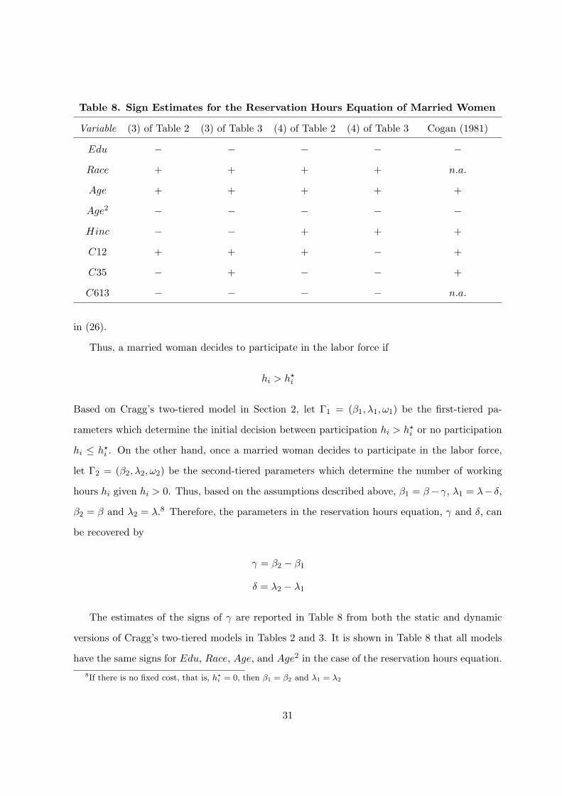
Table 8. Sign Estimates for the Reservation Hours Equation of Married Women

Variable (3) of Table 2 (3) of Table 3 (4) of Table 2 (4) of Table 3 Cogan (1981)

Edu − − − − −

Race + + + + n.a.

Age + + + + +

Age2 − − − − −

Hinc − − + + +

C12 + + + − +

C35 − + − − +

C613 − − − − n.a.

in (26).

Thus, a married woman decides to participate in the labor force if

hi > h⋆i

Based on Cragg’s two-tiered model in Section 2, let Γ1 = (β1, λ1, ω1) be the first-tiered pa-

rameters which determine the initial decision between participation hi > h⋆i or no participation

hi ≤ h⋆i . On the other hand, once a married woman decides to participate in the labor force,

let Γ2 = (β2, λ2, ω2) be the second-tiered parameters which determine the number of working

hours hi given hi > 0. Thus, based on the assumptions described above, β1 = β−γ, λ1 = λ− δ,

β2 = β and λ2 = λ.8 Therefore, the parameters in the reservation hours equation, γ and δ, can

be recovered by

γ = β2 − β1

δ = λ2 − λ1

The estimates of the signs of γ are reported in Table 8 from both the static and dynamic

versions of Cragg’s two-tiered models in Tables 2 and 3. It is shown in Table 8 that all models

have the same signs for Edu, Race, Age, and Age2 in the case of the reservation hours equation.

8If there is no fixed cost, that is, h⋆i = 0, then β1 = β2 and λ1 = λ2

31

The husband’s income has a negative impact on the reservation hours equation in the random

effects Cragg two-tiered model (model (3) of Tables 2 and 3), but it has a positive impact on the

reservation hours equation in the correlated random effects models. In comparing the results of

the correlated random effects models in Table 8 with the estimation results of the reservation

hours function in Cogan (1981), the signs are the same for the wife’s education, the husband’s

earnings and the wife’s age. In addition, it is found in Table 8 that black women might have

higher reservation hours than white women. Also shown in Cogan’s estimation results is that

the number of children aged between 0 and 6 years will have a positive impact on the reservation

hours. For the correlated random effects two-tiered models in Table 8, although the number

of children aged between 1 and 2 years old will increase the reservation hours, the number of

children aged between 3 and 13 years old will decrease the reservation hours for married women.

3.6 Monte Carlo Experiments

In this subsection, a small number of Monte Carlo experiments are performed in order to provide

supporting evidence for the estimation results of Cragg’s two-tiered models. For each experi-

ment, the Monte Carlo data set is generated from two-tiered models and estimated by both

standard Tobit and two-tiered models. The initial conditions problems are also investigated

using Heckman’s approach.

In order to replicate the variation in the empirical data, the exogenous variable in the Monte

Carlo experiments, Zit, is a standardized composite variable generated from the data used in the

empirical analysis. Specifically, Zit = (Xitθ−Z)/σZ , where Xit is a vector of variables in Table

3, and θ is a vector of parameters estimated in the first tier of Model (4) in Table 3. Moreover,

Z =

∑N

i=1

∑T

t=1Xitθ

NT , and σZ =√σ2d + σ2

u/(1− ζ2), where σ2d, σ

2u and ζ are estimated in Model

(4) of Table 3.9

The Monte Carlo data sets are generated from the two-tiered models. In the first tier, the

probability of a zero is given by a probit model with a parameter vector β10 for an intercept, β11

for an exogenous variable Zit, and λ1 for a lagged dependent variable. On the second tier, the

density of the dependent variable conditional on being a positive observation is assumed to be

9A similar approach is used in the Monte Carlo experiments in Hyslop (1999).

32

truncated at zero with a parameter vector β20 for an intercept, β21 for an exogenous variable Zit,

and λ2 for a lagged dependent variable. The error terms uit and di are assumed to satisfy the

conditions in (3) and are assumed to be normally distributed. The covariance matrix is assumed

to follow the random effects plus AR(1) specification with σ2u = 0.5, σ2

d = 0.5 and ζ = 0.5.

The simulation estimator is obtained by maximizing the simulated log-likelihood function of the

Monte Carlo data set. In all Monte Carlo experiments, the number of individuals, N , is set

at 1,000, and each individual is observed in five time periods. Each data generating process is

simulated 20 times, and estimated by using the GHK simulation estimators with 10 simulation

draws. The Monte Carlo data sets are estimated by both Cragg’s two-tiered model and the

standard Tobit model.

The first two Monte Carlo experiments are conducted without an initial conditions problem

in Table 9. That is, all the data are observed from the beginning of the data generating process,

and it is assumed that there is no lagged dependent variable in the first period. The censoring

frequency is 0.4328 for experiment I and is 0.5091 for experiment II in Table 9. The mean,

median, 5th percentile, 95th percentile, and standard error (S.E.) of the simulation estimators

are reported for each Monte Carlo experiment. In experiment I of Tables 9 and 10, the slope

parameters in the first and second tiers have the same sign but have different magnitudes. On

the other hand, the slope parameters in the first and second tiers have the same magnitude but

have different signs in experiment II of Tables 9 and 10.

It is shown in Table 9 that the estimators of β and λ for the Tobit model tend to be the

average of the true parameters from the first and second tiers. For the two-tiered estimators,

the signs of the parameters are all correctly estimated, although they tend to underestimate

most of the parameters. For the estimation of σ2u, σ

2d and ζ, the two-tiered estimators tend to

underestimate them. On the other hand, Tobit estimators tend to overestimate σ2u, σ

2d and ζ

due to the restrictions on the parameters imposed by the Tobit models.

For the investigation of the initial conditions problem, it is assumed that the Monte Carlo

data are observed from the middle of the data generating process. The Monte Carlo data set is

generated using the true parameter values in Table 10 for 9 periods, but only the last 5 periods

of the data are observed and used in the estimation. The Heckman approach is used to deal

33

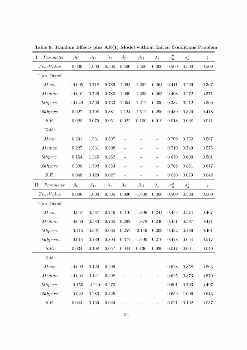
Table 9. Random Effects plus AR(1) Model without Initial Conditions Problem

I: Parameter β10 β11 λ1 β20 β21 λ2 σ2u σ2

d ζ

TrueV alue 0.000 1.000 0.500 0.500 1.500 0.300 0.500 0.500 0.500

Two-Tiered:

Mean -0.005 0.718 0.789 1.094 1.352 0.264 0.411 0.269 0.367

Median -0.001 0.726 0.780 1.099 1.353 0.265 0.408 0.272 0.371

5thperc. -0.049 0.590 0.733 1.054 1.212 0.230 0.384 0.212 0.309

95thperc. 0.027 0.798 0.881 1.124 1.512 0.296 0.439 0.320 0.418

S.E. 0.028 0.075 0.051 0.022 0.100 0.019 0.018 0.038 0.041

Tobit:

Mean 0.231 1.531 0.307 - - - 0.709 0.752 0.567

Median 0.227 1.531 0.308 - - - 0.710 0.749 0.575

5thperc. 0.154 1.345 0.262 - - - 0.670 0.600 0.501

95thperc. 0.308 1.702 0.353 - - - 0.768 0.851 0.617

S.E. 0.048 0.129 0.027 - - - 0.030 0.079 0.042

II: Parameter β10 β11 λ1 β20 β21 λ2 σ2u σ2

d ζ

TrueV alue 0.000 1.000 0.500 0.000 -1.000 0.300 0.500 0.500 0.500

Two-Tiered:

Mean -0.067 0.587 0.746 0.310 -1.896 0.241 0.455 0.574 0.467

Median -0.060 0.580 0.760 0.292 -1.878 0.240 0.451 0.587 0.471

5thperc. -0.115 0.397 0.660 0.257 -2.146 0.209 0.432 0.486 0.401

95thperc. -0.014 0.739 0.804 0.377 -1.690 0.270 0.478 0.654 0.517

S.E. 0.034 0.108 0.057 0.044 0.136 0.020 0.017 0.061 0.040

Tobit:

Mean -0.092 0.120 0.299 - - - 0.628 0.858 0.563

Median -0.094 0.141 0.298 - - - 0.625 0.873 0.570

5thperc. -0.156 -0.120 0.270 - - - 0.601 0.703 0.497

95thperc. -0.022 0.280 0.325 - - - 0.659 1.006 0.613

S.E. 0.044 0.139 0.024 - - - 0.021 0.102 0.037

34

with the initial conditions problem.

The censoring frequency is 0.4093 for experiment I and is 0.4895 for experiment II in Table

10. Like Table 9, the estimations of β and λ for the Tobit model in Table 10 tend to be the

average of the true parameters from the first and second tiers. Moreover, the Tobit estimators

tend to overestimate σ2u, and σ2

d and ζ. Overall, the two-tiered estimators perform equally well

with or without the initial conditions problem.

It is indicated in the Monte Carlo experiments that when the true data generating process is

determined by two different sets of parameters, Cragg’s two-tiered estimators are preferable to

the traditional Tobit estimators since the Tobit estimators tend to perform like the average of the

first- and second-tiered parameters. Thus, when the true data generating process is unknown,

Cragg’s two-tiered estimators may be better choices than the Tobit estimators.

4 Conclusion

This paper has proposed a computationally practical simulation estimator for dynamic panel

Tobit models as well as Cragg’s two-tiered dynamic panel Tobit models based on maximizing

simulated log-likelihood functions. The proposed Cragg two-tiered simulation estimators are

then applied to study married women’s labor supply. The rich dynamic structures of the labor

supply of married women have been identified through the proposed simulation estimators.

By applying the two-tiered dynamic panel Tobit model based on the correlated random ef-

fects approach, it is found that education has a positive impact not only on the labor force

participation decision, but also on the hours worked decision which is conditional on the par-

ticipation. However, race may only have a statistically significant positive impact on the hours

worked decision that is conditional on the participation, but not on the labor force participation

decision. In addition, children aged between 6 and 13 years old may have a negative impact on

the hours worked decision for married women that is conditional on the participation. However,

these children may provide some positive incentives for married women to participate in the

labor force. Furthermore, the hypothesis that the fertility decision is exogenous and the hypoth-

esis that the husband’s income is exogenous to the married women’s labor supply function are

35

Table 10. Random Effects plus AR(1) Model with Initial Conditions Problem

I: Parameter β10 β11 λ1 β20 β21 λ2 σ2u σ2

d ζ

TrueV alue 0.000 1.000 0.500 0.500 1.500 0.300 0.500 0.500 0.500

Two-Tiered:

Mean 0.232 1.080 0.582 1.239 1.718 0.067 0.472 0.410 0.629

Median 0.233 1.076 0.582 1.237 1.780 0.065 0.478 0.391 0.638

5thperc. 0.157 0.906 0.507 1.179 1.502 0.022 0.438 0.326 0.580

95thperc. 0.301 1.262 0.648 1.304 1.859 0.111 0.494 0.513 0.669

S.E. 0.057 0.125 0.055 0.047 0.130 0.030 0.021 0.071 0.034

Tobit:

Mean 0.474 1.901 0.077 - - - 0.703 0.728 0.758

Median 0.476 1.898 0.076 - - - 0.699 0.744 0.764

5thperc. 0.406 1.658 0.048 - - - 0.663 0.343 0.696

95thperc. 0.555 2.098 0.106 - - - 0.748 1.029 0.809

S.E. 0.050 0.148 0.023 - - - 0.025 0.229 0.035

II: Parameter β10 β11 λ1 β20 β21 λ2 σ2u σ2

d ζ

TrueV alue 0.000 1.000 0.500 0.000 -1.000 0.300 0.500 0.500 0.500

Two-Tiered:

Mean 0.049 0.455 0.498 0.367 -1.883 0.069 0.493 0.725 0.665

Median 0.054 0.435 0.484 0.361 -1.888 0.067 0.496 0.733 0.664

5thperc. -0.009 0.344 0.431 0.285 -2.049 0.041 0.453 0.543 0.618

95thperc. 0.131 0.634 0.567 0.497 -1.727 0.098 0.524 0.867 0.720

S.E. 0.047 0.102 0.053 0.064 0.118 0.019 0.026 0.111 0.038

Tobit:

Mean 0.045 0.084 0.074 - - - 0.636 0.866 0.756

Median 0.031 0.077 0.081 - - - 0.638 0.915 0.758

5thperc. -0.029 -0.089 0.028 - - - 0.601 0.487 0.695

95thperc. 0.142 0.253 0.109 - - - 0.666 1.126 0.811

S.E. 0.053 0.129 0.024 - - - 0.024 0.226 0.039

36

both rejected in the dynamic and static two-tiered models.

Acknowledgements

I would like to thank Arthur Goldberger, Bruce Hansen, and Gautam Tripathi for their helpful

discussions and suggestions. I am especially indebted to Yuichi Kitamura for his encouragement

and invaluable guidance. I would also like to thank Professor John Rust and two anonymous

referees for their useful comments and suggestions. All errors which remain are mine.

References

Browning, M. 1992, Children and household economic behavior, Journal of Economic Literature

XXX, 1435-1475.

Chamberlain, G., 1984, Panel data, in: Z. Griliches and M.D. Intriligator, eds., Handbook of

econometrics, Vol. 2 (Elsevier Science Publishers BV, Amsterdam) 1247-1318.

Cogan, J., 1981, Fixed costs and labor supply, Econometrica 49, 945-963.

Cragg, J. 1971, Some statistical models for limited dependent variables with application to the

demand for durable goods, Econometrica 39, 829-844.

Eckstein, Z. and K. Wolpin, 1989, Dynamic labor force participation of married women and

endogenous working experience, Review of Economic Studies 56, 375-390.

Gourieroux, C. and A. Monfort, 1993, Simulation-based inference: a survey with special refer-

ence to panel data models, Journal of Econometrics 59, 5-33.

Hajivassiliou, V., 1994, A simulation estimation analysis of the external debt crises of developing

countries, Journal of Applied Econometrics 9, 109-132.

Hajivassiliou, V., 1993, Simulation estimation methods for limited dependent variable mod-

els, In: G.S. Maddala, C.R. Rao and H.D. Vinod, eds., Handbook of statistics Vol. 11,

Amsterdam: North-Holland, 519-543.

37

Hajivassiliou, V., 1987, The external debt repayments problems of LDC’s: an econometric

model based on panel data, Journal of Econometrics 36, 205-230.

Hajivassiliou, 1985, unpublished MIT Ph.D. thesis.

Hajivassiliou, V. and D. McFadden, 1998, The method of simulated scores for estimating limited

dependent variable models, Econometrica 66, 863-896.

Hajivassiliou, V., D. McFadden, and P. Ruud, 1996, Simulation of multivariate normal rectan-

gle probabilities and their derivatives: theoretical and computational results, Journal of

Econometrics 72, 85-134.

Heckman, J., 1979, Sample selection bias as a specification error, Econometrica 47, 153-162.

Heckman, J., 1981, Statistical models for discrete panel data, In: C.F. Manski and D. McFad-

den, eds., Structural analysis of discrete panel data with econometric applications (MIT

press) 114-178.

Heckman, J., and T. MaCurdy 1980, A life cycle model of female labour supply, Review of

Economic Studies 47, 47-74.

Heckman, J., and T. MaCurdy 1980, Corrigendum on a life cycle model of female labour supply,

Review of Economic Studies 49, 659-660.

Honore, B., 1993, Orthogonality conditions for Tobit models with fixed effects and lagged

dependent variables, Journal of Econometrics 59, 35-61.

Honore, B. and L. Hu, 2004, Estimation of cross sectional and panel data censored regression

models with endogeneity, Journal of Econometrics 122, 293-316.

Hu, L., 2002, Estimation of a censored dynamic panel data model, Econometrica 70, 2499-2517.

Hyslop, D.R., 1999, State dependence, serial correlation and heterogeneity in intertemporal

labor force participation of married women, Econometrica 67, 1255-1294.

38

Jakubson, G., 1988, The sensitivity of labor-supply parameter estimates to unobserved indi-

vidual effects: fixed- and random-effects estimates in a nonlinear model using panel data,

Journal of Labor Economics 6, 302-329.

Keane, M., 1994, A computationally practical simulation estimator for panel data, Economet-

rica 62, 95-116.

Lerman, S. and C. Manski, 1981, On the use of simulated frequencies to approximate choice

probabilities, In: C.F. Manski and D. McFadden, eds., Structural analysis of discrete panel

data with econometric applications (MIT press), 305-319.

Lin, T. and P. Schmidt, 1984, A test of the Tobit specification against an alternative suggested

by Cragg, Review of Economics and Statistics 66, 174-177.

McFadden, D., 1989, A method of simulated moments for estimation of discrete choice models

without numerical integration, Econometrica 57, 995-1026.

Mroz, T., 1987, The sensitivity of an empirical model of married women’s hours of work to

economic and statistical assumptions, Econometrica 55, 765-799.

Mundalk, Y., 1978, On the pooling of time-series and cross-section data, Econometrica 46,

69-85.

Rust, J., 1994, Structural estimation of Markov decision processes, in: R. Engle and D. McFad-

den, eds., Handbook of econometrics, Vol. 4 (Elsevier Science Publishers BV, Amsterdam)

3082-3143.

Wooldridge, J., 2002, Econometric analysis of cross section and panel data (MIT Press).

39