ansi s1.11 1986(asa 65-1986)
TRANSCRIPT
ANSI Sl.ll-1986 (ASA 65-l 986)
[Revision of ANSI Sl.ll-1966(R1976)]
Standards Secretariat Acoustical Society of America 335 East 45th Street New York, New York 10017-3483
AMERICAN NATIONAL STANDARD Specification for Octave-Band and Fractional-Octave-Band Analog and Digital Filters
A%STRACT
This standard provides performance requirements for fractional-octave-band band- pass filters, including, in particular, octave-band and one-third-octave-band filters. Basic requirements are given by equations with selected empirical constants to estab- lish limits on the required performance. The requirements are applicable to passive or active analog filters that operate on continuous-time signals, to analog and digital filters that operate on discrete-time signals and to fractional-octave-band analyses synthesized from narrow-band spectral components. Filter designs are described by an Order number which is usually related to the number of poles in the analog proto- type low-pass filter or the number of pole pairs in the analog prototype bandpass filter. The overall accuracy of a filter set is described by a Type number, which is determined by the accuracy of a measurement of a white noise signal, and a required Sub-Type letter, which is determined by the accuracy of the measurement of signals with moderate spectral slopes. Four accuracy grades are allowed: the most accurate for precise analog and digital filters; the next for filters achievable with the technology of the 1980s. The two least accurate grades describe filters which meet the require- ments of Sj .l l-l 966. An Appendix is included for reference to terminology used in digitial signal processing.
Published by the American Institute of Physics for the Acoustical Society of America
AMERICAN NATIONAL STANDARDS ON ACOUSTICS
The Acoustical Society of America holds the Secretariat for Accredited Standards Committees Sl on Acoustics, S2 on Mechanical Shock and Vibration, S3 on Bioacoustics, and S12 on Noise. Standards developed by these committees, which have wide representation from the technical community (manufacturers, consumers, and general-interest representatives), are published by the American Institute of Physics for the Acoustical Society of America as American National Standards after approval by their respective standards committees and the American National Standards Institute.
These standards are developed as a public service to provide standards useful to the public, industry, and consumers, and to Federal, State, and local governments.
This standard was approved by the American National Standards Institute as ANSI Sl.ll-1986 on 16 July 1986.
An American National Standard implies a consensus of those substantially concerned with its scope and provisions. An American National Standard is intended as a guide to aid the manufacturer, the consumer, and the general public. The existence of an American
National Standard does not in any respect preclude anyone, whether he has approved the standard or not, from manufacturing, marketing, purchasing, or using products, processes, or procedures not conforming to the standard. American National Standards are
subject to periodic review and users are cautioned to obtain the latest editions.
Caution Notice: An American National Standard may be revised or withdrawn at any time. The procedures of the American National
Standards Institute require that action be taken to affirm, revise, or withdraw this standard no later than five years from the date of
publication.
Copyright @ 1986 by the Acoustical Society of America. No portion of this publication may be quoted or reproduced in any form without permission of the
Acoustical Society of America
FOREWORD
[This Foreword is for information only and is not a part of American National Standard Specification for Octave-Band and Fractional-
Octave-Band Analog and Digital Filters, S1.l 1-1986 (ASA Catalog No. 65-1986J.J
This standard was developed under the jurisdiction of Accredited Standards Committee Sl using the American National Standards Institute (ANSI) Standards Committee Procedure. The Acoustical Society of America holds the Secretariat for Accredited Standards Committee Sl . This standard was approved for publication by Accre- dited Standards Committee Sl and by the American National Standards Institute.
This standard is a revision of ANSI Sl.l l-1966 (R19761, Octave, Half-Octave, and Third-Octave Band Filter Sets. This standard differs from the 1966 version in several ways principally related to advances in the state-of- the-art. The design complexity of a bandpass filter is now described by an Order number instead of a Class number. The Order number is usually related to the number of poles in the prototype analog low-pass filter
design. This standard also introduces Type and Sub-Type designations to describe the accuracy of a measur-
ment for signals having several spectral slopes, including white noise as a reference. As in the previous stan- dard, performance requirements are established by equations with selected empirical constants to establish limits. Two type numbers are established to cover octave-band and one-third-octave-band filters which meet the requirements of Sl .l l-1966. Digital as well as analog filters are covered by this standard.
Accredited Standards Committee Sl, under whose jurisdiction this standard was developed, has the following scope:
Standards, specifications, methods of measurement and test, and terminology, in the fields of physical acoustics, including architec- tural acoustics, electroacoustics, sonics and ultrasonics, and underwater sound, but excluding those aspects which pertain to safety, tolerance, and comfort.
At the time this standard was submitted to Accredited Standards Committee Sl, for final approval, the mem-
bership was as follows:
E. H. Toothman, Chairman D. L. Johnson, Vice-Chairman A. Brenig, Secretary
Acoustical Society of America l T. F. Embleton, D. L. Johnson
(A/t) Air-Conditioning and Refrigeration institute . R. Harold, H. C.
Skarbek (A/f) American Industrial Hygiene Association l C. C. Bohl American Iron & Steel Institute E. H. Toothman. P. A. Her- nandez (A/t) AT&T’. S. R. Whitesell, R. M. Sachs (A/t)
Audio Engineering Society l L. W. Sepmeyer, M. R. Chial (A/t) Bruel & Kjaer Instruments, Inc. l G. C. Michel Computer & Business Equipment Manufacturers Associa- tion . L. F. Luttrell
Exchange Telephone Group Committee (ETCC) l J. L. Sullivan,
0. 1. Gusella (A/t)
Larson-Davis Laboratories l D. L. Johnson, L. Davis (A/t)
National Bureau of Standards l S. L. Yaniv
National Council of Acoustical Consultants l A. P. Nash, C. W. Kamperman (A/r) Scantek, Inc. . R. J. Peppin U.S. Army Aeromedical Research Laboratory e B. Mozo, J. H.
Patterson; Jr. (A/[) U.S. Army Communication Electronics Command . M. S.
Mayer U.S. Army Human Engineering laboratory l J. Kalb, G. Car- inther (A/t) U.S. Department of the Air Force . R. McKinley U.S. Department of the Army, Environmental Office l P. D. Schemer, R. Raspet (A/t)
. . III
FOREWORD
Individual experts of the Sl Committee were:
L. Batchelder .
S. L. Ehrlich K. M. Eldred
D. R. Flynn
R. 5. Gales W. J. Galloway
E. E. Gross, Jr.
R. M. Guernsey A. P. C. Peterson R. K. Hillquist L. W. Sepmeyer R. Huntley W. R. Thornton W. W. Lang H. E. von Cierke C. C. Mating, Jr. 6. S. K. Wong A. H. Marsh R. W. Young
The membership of Working Group 51-S Octave-band and Fractional-octave-band Analog and Digital Filters, which assisted the Accredited Standards Committee Sl in the preparation of this standard, had the following membership:
L. W. Sepmeyer, Chairman
D. Cox
A. H. Gray, Jr.
F. j. Harris
J. F. Kaiser
A. H. Marsh
C. C. Michel
A. P. Nash
B. E. Walker
G. S. K. Wong
Suggestions for improvement of this standard will be welcomed. They should be sent to the Standards Man- ager, Standards Secretariat, Acoustical Society of America, 335 East 45th Street, New York, NY 10017-3483.
CONTENTS
0 1NTRODUCTlON.. ................................................................................................................................ 1
0.1 General Objective ......................................................................................................................... 1
0.2 Spectrum Analysis.. ........................................................................................................................ 1
0.3 Selection of Frequency Bands.. ...................................................................................................... 1
0.4 Designation of Filter Sets.. .............................................................................................................. 1
0.5 Designation of Filter Characteristics ................................................................................................ 1
0.6 Specification of Filter Characteristic Shape.. ................................................................................... 2
0.7 Phase and Transient Response.. ..................................................................................................... 2
0.8 Influence of External Conditions.. ................................................................................................... 2
0.9 Extension to Infrasonic and Ultrasonic Frequencies.. ...................................................................... 2
1 PURPOSE .............................................................................................................................................. 3
2 SCOPE ................................................................................................................................................... 3
3 APPLICATIONS.. ................................................................................................................................... 3
4 STANDARDS REFERRED TO IN THIS DOCUMENT.. .......................................................................... 3
4.1 American National Standards.. ....................................................................................................... 3
4.2 International Standards .................................................................................................................. 3
5 DEFINITIONS.. ...................................................................................................................................... 4
6 REQUIREMENTS.. .................................................................................................................................. 4
6.1 Filter Sets.. ....................................................................................................................................... 4
6.2 Reference Frequencies .............................................. ..:. .................................................................. .4
6.3 Exact Midband Frequencies ............................................................................................................. 4
6.4 Bandedge Frequencies .................................................................................................................... .6
6.5 Reference-Filter Bandwidths and Bandwidth Quotients ................................................................... .6
6.6 Attenuation Characteristics of individual Filters ................................................................................ 6
6.7 Effective Bandwidth ........................................................................................................................ .7
6.8 Passband Uniformity.. ..................................................................................................................... .9
6.9 Variation of Reference Passband Attenuation.. ................................................................................. 9
6.10 Removal of Filters from Circuit ....................................................................................................... .9
6.1 1 Terminating Impedances.. ................................................................................................................ 9
6.1 2 Maximum Input Signal ..................................................................................................................... 9
6.13 Linearity.. ......................................................................................................................................... 9
6.14 Nonlinear or Harmonic Distortion.. .................................................................................................. 9
6.15 Transient Response .......................................................................................................................... 9
6.16 Phase and Group Delay Response .................................................................................................. .9
6.1 7 Dynamic Range ............................................................................................................................... 9
6.18 Analysis of Nonstationary Signals.. ................................................................................................. 10
6.19 Sensitivity to Extefnaf Conditions ................................ . ..... . ........ .: ................................................... 10
7 SAMPLED DATA SYSTEMS.. ................................................................................................................ 11
7.1 Analog Filters.. ............................................................................................................................... 11
7.2 Digital Filters .................................................................................................................................. 1 1
V
vi
B METHOD OF TEST .............................................................................................................................. 11
8.1 Attenuation Characteristic.. ........................................................................................................... .I 1
8.2 Dynamic Range ............................................................................................................................. 1 2
8.3 Phase-Response Characteristic (Optional). ...................................................................................... 12
APPENDIX A: PERFORMANCE Of BUTTERWORTH BANDPASS FILTERS ........................................... 12
APPENDIX B: PHASE AND GROUP DELAY RESPONSE OF BU’TTERWORTH BANDPASS FILTERS.. ............................................................................................................................ 15
APPENDIX C: ATTENUATION FOR ORDER 3 OCTAVE-BAND AND ONE-THIRD-OCTAVE-BAND FILTERS.. ............................................................................................................................ 17
APPENDIX D: SWITCHED CAPACITOR FILTERS ................................................................................... 18
APPENDIX E: TERMINOLOGY IN DIGITAL SIGNAL PROCESSING.. .................................................... 19
FIGURES
FIG. 1 Schematic of two-voltmeter test arrangement ......................................................................... 1 1
FIG. Bl Phase response and normalized group delay for an Order 3 reference Butterworth octave-band filter.. .................................................................................................................. 1 5
FIG. 82 Phase response and normalized group delay for an Order 3 reference Butterworth one-third-octave-band filter .................................................................................................... 16
TABLES
TABLE 1 Listing of filter bands to be provided by a set of filters.. ........................................................ 5
TABLE 2 Nominal bandedge frequency ratios and filter bandwidth ratios for Order 3 octave-band and one-third-octave-band filters .......................................................................................... 6
TABLE 3 Criteria for selecting Type number ........................................................................................ 7
TABLE 4 Criteria for selecting Sub-Type letter ..................................................................................... 7
TABLE Al Performance of Butterworth bandpass filters.. ....................................................................... 13
TABLE A2 Bandwidth error for analog Butterworth bandpass filters ....................................................... 14
TABLE Cl Attenuation for Order 3 Type 1-X and Type 2-X octave-band and one-third-octave band Butterworth filters.. ............................................................................ 17
TABLE C2 Frequency ratios for Order 3 Type 1-X and Type 2-X octave-band and one-third octave-band Butterworth filters.. ............................................................................ 18
American National Standard Specification for Octave-Band and Fractional-Octave-Band Analog and Digital Filters
0 INTRODUCTION
0.1 General Objective
The spectral distribution of the power in sound and vibration signals is determined for various purposes, Those purposes include scientific, technical, legal, and artistic requirements. The types of signals involved cover wide variations of waveform, amplitude, fre- quency content, duration, coherence, etc. Suitable standards are required for spectrum analysis systems so that satisfactorily uniform results can be obtained from any analyzer that meets the standard for its Type.
0.2 Spectrum Analysis
Frequency-selective networks used in spectrum analyzers fall into two broad classes: ( 1) constant- bandwidth filters where the difference between the up- per and lower bandedge frequencies remains constant over the tuning range of the analyzer; and (2) con- stant-percentage-bandwidth filters, where the ratio of the upper bandedge frequency to the lower bandedge frequency is constant over the tuning range, e.g., frac- tional-octave-band filters.
0.3 Selection of Frequency Bands
An octave-band or fractional-octave-band filter has bandedge frequencies that have a fixed relationship to the geometric-mean frequency of the passband. For convenience, filters are identified by the standard pre- ferred frequencies, or, for octave-band and one-third- octave-band filters, by the standard .band numbers specified in ANSI S1.6-1984.
The performance requirements of this standard, while directed mainly at octave-band and one-third- octave-band filters may be applied to any fractional- octave-band filter. For analog filters, it is often desir- able to base the filter design on geometric mean frequencies that are related by fractional powers of ten, while for digital filters and switched capacitor filters, geometric mean frequencies based on powers of two may be more convenient.
0.4 Designation of Filter Sets
For many purposes, it is sufficient for a filter set to contain a particular number of filters covering the usu- al audio-frequency range. However, other applications
may require fewer or additional filters to cover a range less than or greater than the usual range. To permit this standard to cover a wide range of applications, fil- ter sets of three designations have been delineated for use in the audio-frequency range: i.e., Restricted Range, Extended Range,- and Optional Range.
0.5 Designation of Filter Characteristics
During the 197Os, advances in technology and the operation of the market place resulted in what was then known as the Class II octave-band filter and Class III third-octave-band filter becoming de facto in- dustry standards. During that time, few, if any, Class I octave-band filters were offered for sale. Also, the half- octave-band filter became extinct. Since the design goal characteristics in Sl. 11-1966 for both the Class II octave-band and Class III third-octave-band filters were based on the third-order Butterworth or maxi- mally flat filter characteristic, this standard bases filter complexity designations on the order of the prototype low-pass filter design or the number of pole pairs or resonators in the bandpass filter design. Thus the one- third-octave-band filter designation number remains the same.
However, to avoid possible confusion, the term Class was changed to Order, the term commonly used in filter design engineering. Thus, a third-order Butter- worth octave-band filter that was previously called a Class II octave-band filter is now designated as an Or- der 3 octave-band filter. Stated in another way, the fil- ter Order designation is directly correlated with the number of resonators or pole pairs in an analog filter design including the prototype for an infinite impulse response or recursive digital filter. Hence, a single tuned circuit would be designated an Order 1 filter while an ideal, or brick-wall, filter would be designated an Order infinity filter. Also, roman numerals have been replaced by arabic numerals for the Order num- ber.
The choice of filter Order to be used for a given measurement depends on the accuracy required. For many applications, any set of Order 3 filters is suffi- cient. For some applications (e.g.; determining the pressure spectrum level of a short duration impulsive sound or the true one-third-octave-band sound-pres- sure levels of a noise signal that has propagated a mod- erate distance through an absorptive medium), spec- trum slopes ranging from - 30 to - 90 decibels per
octave can occur and filters of Order greater than 3 the analog of the time-mean-square sound pressure or may be warranted. For general usage with sound level vibration signal. Since that quantity is independent of meters, octave-band and one-third-octave-band filters the relative phase among spectral components, the should be not less than Order 3. phase response characteristic of a filter set is of no con-
cern and therefore has not been specified. Also, devia-
0.6 Specificatioli of Filter Characteristic tions from the inherent phase and transient responses of an analog filter will result from the allowed manu-
Shape facturing tolerances on component values, making it Specification of the attenuation characteristic of a impractical to specify closely filter characteristics, par-
filter by a small number of straight-line segments often ticularly the phase response. complicates the design of economical real filters which do not have attenuation characteristics approximating
Distortion of the waveform of a transient signal in-
long straight-line segments. For this standard, the troduced by phase nonlinearity of a filter should have
limiting attenuation characteristics are specified by negligible effect on the indicated filtered level. How-
mathematical expressions based upon the design for- ever, phase distortion can affect the measurement of
mulas of maximally flat bandpass filters, This choice the peak level of a complex waveform. When a filter of
makes it easier for the designer to provide filters that any practical design is excited by a short-duration
meet the requirements for attenuation characteristics, transient and the output is displayed on an oscillo-
effective bandwidth, and nominal midband frequency. scope, a transient response will be observed in the form of damped oscillations called “ringing.” Limits are
It was considered feasible for the tolerance limits in placed on the magnitude and duration of such oscilla- this standard to be more stringent than in the 1966 tions. version. However, for those applications where techni- cal and economic considerations do not require in- 0.8 Influence of External Conditions creased accuracy, the previous 10% bandwidth error limit is retained and three additional categories of ef- , When filter sets made according to this standard
fective bandwidth accuracy are established. In confor- are to be used with portable instruments such as sound
mance with the usage of American National Standard level meters, the filter set should be designed to meet
Specification for Sound Level Meters, ANSI S1.4- the same environmental conditions specified for those
1983, the basic accuracy of the response of a filter to instruments. The range of environmental conditions
white noise (relative to the response of a correspond- specified in ANSI S1.4-1983 is incorporated in this
ing ideal filter) is designated by a Type number, with standard.
increasing error being designated by a larger number.
The bandwidth error of a filter depends upon its at- tenuation at the bandedges, the slope of the attenu-
0.9 Extension to Infrasonic and Ultrasonic
ation characteristic in the transition bands, and the Frequencies
spectrum slope of the input noise spectrum. To accom- modate various practical applications, an additional
The 1966 version of this standard was intended to
component has been added to the bandwidth error apply primarily to measurement of sound or vibration
Type designator to apprise the user of the inherent signals with a frequency content within the usual
bandwidth error for analysis of sound or vibration sig- range of human audibility, commonly called the
nals having moderately steep spectral slopes. audio-frequency range. For many applications, it is de- sirable to extend the frequency range downward to in-
A mathematical equation is given to specify the de- frasonic frequencies or upward to ultrasonic frequen-
sign reference attenuation characteristic for any filter. cies.
That equation, together with equations defining filter bandwidth and filter bandwidth quotient, constitutes
This standard permits the use of either of two geo-
the basic performance parameters for any filter cov- metric series for specifying midband frequencies. One
ered by this standard. The equations are unambiguous series is a fractional-octave series based on powers of
and not subject to errors of curve plotting, interpreta- two; it is referred to as the base two system. The other
tion, or reproduction. series is based on powers of ten; it is referred to as the base ten system.
0.7 Phase and Transient Response In the base ten system, the midband frequencies in- cluded within any 1O:l frequency range are the same
For most sound and vibration measurements, a as within any other 1O:l frequency range except for the time-averaged mean-squared voltage is measured as position of the decimal point. In the base two system,
2 AMERICAN NATIONAL STANDARD
ANSI Sl .I l-1986 3
the midband frequencies are unique and do not have values which repeat.
For measurement of the spectral content of a signal within the audio-frequency range, each of the two se- ries of midband frequencies includes 1 kilohertz exact- ly. [The standard reference frequency of 1 hertz (see ANSI S1.6-1984) is included in the base ten series and in the base two series for filter sets designed for analy- ses of signals in the infrasonic-frequency range.]
As the range of midband frequencies is extended from the audio-frequency range to infrasonic frequen- cies, midband frequencies calculated by the base ten system become increasingly greater than those calcu- lated by the base two system, and vice versa for exten- sion to ultrasonic frequencies.
This standard recommends the use of different ref- erence frequencies to minimize the differences between exact midband frequencies calculated by the base two and base ten systems in the infrasonic- and ultrasonic- frequency regions.
1 PURPOSE
The purpose of this American National Standard Specification for Octave-Band and Fractional-Octave- Band Analog and Digital Filters is to specify the geo- metric mean frequencies, bandedge frequencies, band- widths, attenuation charcteristics, bandwidth error, and other pertinent design parameters for constant- percentage-bandwidth bandpass filters so that spectral analyses made with filters conforming to the specified performance requirements will be consistent within known tolerance limits.
2 SCOPE
The scope of this standard specification includes bandpass filter sets suitable for analyzing electrical sig- nals as a function of frequency. The bandwidth of the filters is a constant percentage of the midband frequen- cy of each filter band. The scope includes passive, ac- tive, and sampled-data bandpass filters obtained by any design realization procedure. All filters, including fractional-octave-band filters synthesized by Discrete Fourier Transform (FFT) techniques shall meet all electrical requirements of the standard. Three frequen- cy ranges of filter sets are described for use in the audio-frequency range where the reference, frequency is one kilohertz. The filters in a filter set may be of any filter design Order. Four filter Types and five Sub- Types are established based on the amount of pass- band ripple and on the bandwidth error for both white noise and random noise having specified moderately sloping spectral distibutions.
3 APPLICATIONS
Bandpass filters designed in conformance with this standard are well suited to the spectral analysis of any electrical signals having energy distributed over a broad frequency range. The resolution of discrete fre- quency components in a signal depends on the Order and bandwidth of the filter and the position of the components within the passband of the filter. The fre- quency range of filters covered by the requirements of this standard may be extended to as low or as high a frequency as desired.
NOTE: Existing filter sets designed to the requirements of earlier versions of this standard may be shown to comply with the applica- ble requirements by performing the specified tests and computa- tions.
4 STANDARDS REFERRED TO IN THIS DOCUMENT
4.1 American National Standards
[When the following American National Standards are superseded by a revision approved by the Ameri- can National Standards Institute, Inc., the revision shall apply. ]
( 1) American National Standard Acoustical Ter- minology (Including Mechanical Shock and Vibra- tion), ANSI Sl.l-1960’(R1976).
(2) American National Standard Specification for Sound Level Meters, ANSI S1.4-1983.
(3) American National Standard Preferred Fre- quencies, Frequency Levels, and Band Numbers for Acoustical Measurements, ANSI S 1.6- 1984.
4.2 International Standards
[When the following publications are superseded by an approved revision, the revision shall apply.]
( 1) “Octave, half-octave, and third-octave-band filters intended for the analysis of sounds and vibra- tion,” International Electrotechnical Commission Recommendation, Publication 225( 1966).
(23 “Acoustics and electroacoustics,“’ Chapter 801 of the International Electrotechnical Vocabulary, In- ternational Electrotechnical Commission Publication IEC 50(801)-1984.
(3) “Preferred frequencies for acoustical measure- ments,” International Organization for Standardiza- tion Recommendation R 266( 1975).
4 AMERICAN NATIONAL STANDARD
5 DEFINITIONS
[Definitions of certain terms are included here for the purposes of this standard. The definitions are con- sistent with those in ANSI Sl.l-1960 (R1976) and those in IEC Publication 50 ( 80 1) - 1984.4
5.1 wave filter (filter): a transducer for separating waves on the basis of their frequency. 5.2 bandpass filter: a wave filter with a single trans- mission band (passband) extending from a lower bandedge frequency greater than zero to a finite upper bandedge frequency. 5.3 bandedge frequencies: the upper and lower cutoff frequency of an ideal bandpass filter. In this standard, the ratio of the upper to the lower cutoff frequency is specified as a fractional power of two. 5.4 filter bandwidth: difference between the upper and lower bandedge frequencies, and, hence, the width of the passband. 5.5 filter bandwidth quotient: figure-of-merit measure of the relative bandwidth, or sharpness, of a bandpass filter and described by the ratio of the midband fre- quency to the bandwidth. 5.6 spectrum: description of the resolution into compo- nents of a function of time, each component having a different frequency and (usually) different amplitude and phase. A continuous spectrum has spectral compo- nents continuously distributed over a range of frequen- cies. A white noise spectrum has a power spectral den- sity (mean-square amplitude per unit frequency) essentially independent of frequency over a specified frequency range. A pink noise spectrum has a spectrum level slope of - 3 dB per octave; hence, equal power per fractional-octave band. 5.7 attenuation: in decibels, reduction in the level of some characteristic of a signal between two stated points in a transmission system relative to a reference attenuation.
NOTES:
( 1) Since this standard is concerned mainly with active analog and digital filters, matched source and load impedances are usually not necessary. Then, attenuation, in decibels, is the difference between the level of a signal applied to the input of a filter and the level of the signal delivered by the filter to its output.
(2) transmission loss is used synonymously with attenuation, as defined above, in connection with filter characteristics.
(3) insertion loss is a term also frequently used in connection with filters. The insertion loss, in decibels, resulting from insertion of a transducer in a transmission system is 10 times the logarithm to the base 10 of the power delivered to that part of the system that will follow the transducer, before insertion, to the power delivered to the same part of the system after its insertion. For passive filters operat- ed between resistive terminating impedances, the insertion loss char- acteristic, employing the minimum insertion loss value, as referent, is the same as the attenuation characteristic.
5.8 terminating impedance: impedances of the external input and output electrical circuits between which the filter is connected. 59 peak-to-valley ripple: difference in decibels be- tween the extremes of a series of minima and maxima of ripple in the attenuation in the passband. See Ap- pendix E, Fig. 14 and paragraph IV (29). 5.10 dynamic range: in decibels, difference between the output level when the maximum-rated band-centered sinusoidal input signal is applied and the wideband (e.g., 5 Hz to 100 kHz) output noise level when the input is terminated with rated impedance and no input signal is applied. 5.11 terminology used in digital signal processing: see Appendix E for additional information on terms used to specify digital filter performance requirements.
6 REQUIREMENTS
6.1 Filter Sets
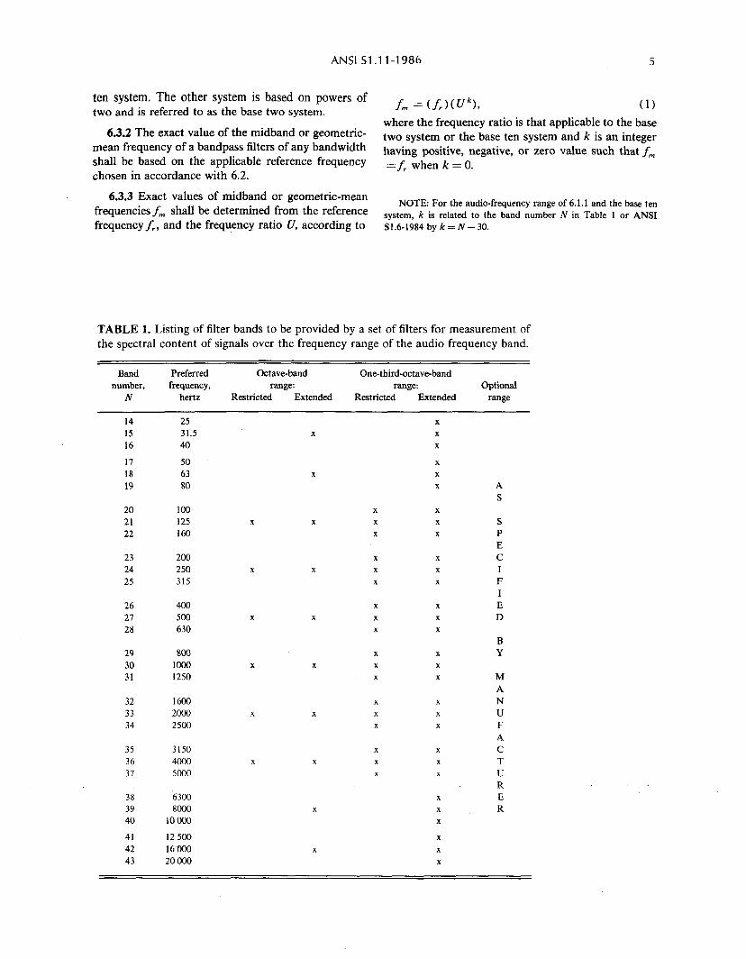
6.1.1 An audio-frequency filter set shall provide a number of filter bands according to the schedules list- ed in Table 1, and shall bear the appropriate Range designation: Restricted Range, Extended Range, or Optional Range.
6.1.2 Octave-band and one-third-octave-band filters shall be identified, or labeled, as shown in Table 1 by the preferred frequencies of ANSI S1.6-1984 and IS0 Recommendation R266( 1975).
6.1.3 Octave-band analyses may be determined by combining the squared outputs of adjacent fractional- octave-band filters.
6.2 Reference Frequencies
When the range of the filter set is predominantly in the audio-frequency range, the reference frequency shall be 1 kilohertz. When the predominant frequency range of the filter set is infrasonic, i.e., preferred fre- quencies less than 20 hertz, the reference frequency of 1 hertz is recommended. When the predominant fre- quency range of the filter set is ultrasonic, i.e., pre- ferred frequencies greater than 31.5 kilohertz, the ref- erence frequency of 1 megahertz is recommended.
6.3 Exact Midband Frequencies
6.3.1 This standard permits two systems for specify- ing the exact geometric-mean frequencies. One system is based on powers of ten and is referred to as the base
ANSI Sl.ll-1986 5
ten system. The other system is based on powers of two and is referred to as the base two system. f, = Lt.WkL (1)
6.3.2 The exact value of the midband or geometric- where the frequency ratio is that applicable to the base
mean frequency of a bandpass filters of any bandwidth two system or the base ten system and k is an integer
shall be based on the applicable reference frequency having positive, negative, or zero value such that f,
chosen in accordance with 6.2. =f, when k=O.
6.3.3 Exact values of midband or geometric-mean frequencies f, shall be determined from the reference
NOTE: For the audio-frequency range of 6.1.1 and the base ten
frequency f,, and the frequency ratio U, according to system, k is related to the band number N in Table 1 or ANSI S1.6-1984 by k = N - 30.
TABLE 1. Listing of filter bands to be provided by a set of filters for measurement of the spectral content of signals over the frequency range of the audio frequency band.
Band Preferred Octave-band One-third-octave-band number, frequency, range: range:
N hertz Restricted Extended Restricted Extended Optional
range
14 15 16
17 18 19
20
21 22
23
24
25
26 21
28
29 30 31
32 33
34
35
36 37
38 39 40
41
42 43
50
63 80
100 125 160
200
250
315
4cm 500 630
800 lC00 1250
1600 2Oca 2500
3150
4ooo 5om
6300 8OtXl
10 CQO
12 500 16000 2oOOcl
x
x
X
X
X
X
x
x
X
X
X
x
X
X
X
x
X
X
X
x
x
A S
X X
x x
x x
x
X
x
x
x
X
x x x
X
X
X
X
X
x
x x x
B Y
M A N U F A C T U R E R
6 AMERICAN NATIONAL STANDARD
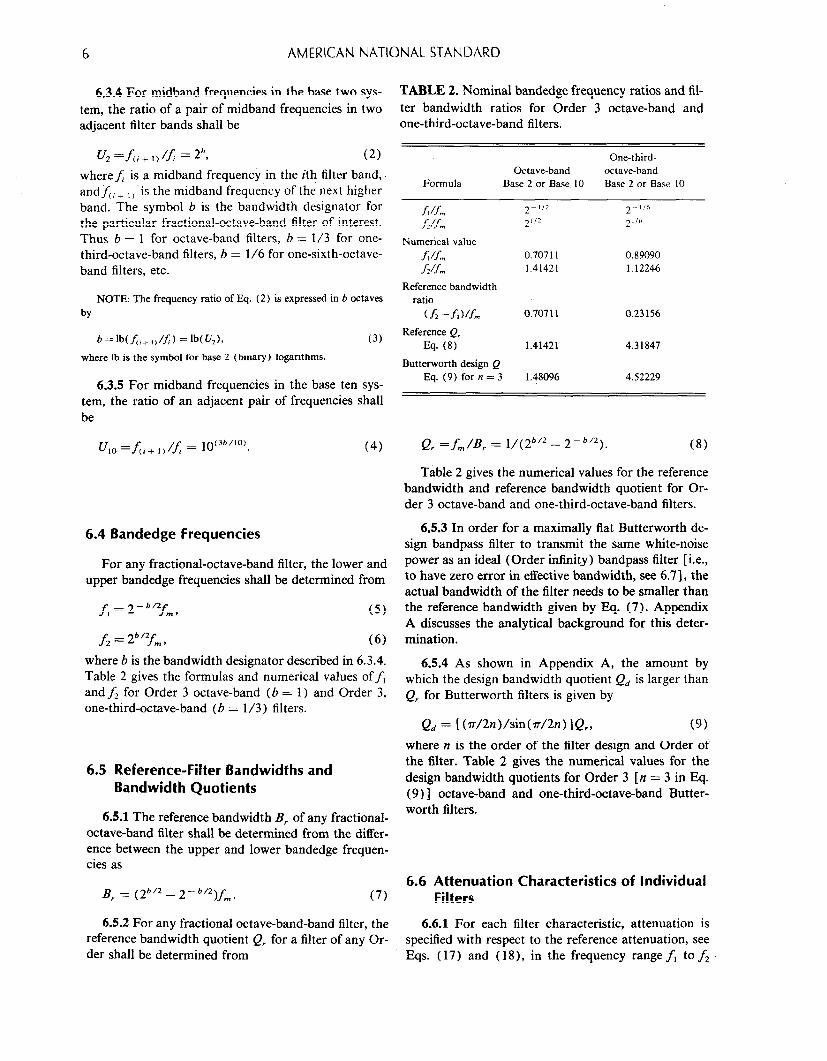
6.3.4 For midband frequencies in the base two sys- TABLE 2. Nominal bandedge frequency ratios and fil- tem, the ratio of a pair of midband frequencies in two ter bandwidth ratios for Order 3 octave-band and adjacent filter bands shall be one-third-octave-band filters.
u2=&i+I)Ui =2b? (2)
wheref; is a midband frequency in the ith filter band,. andA,+ I1 is the midband frequency of the next higher band. The symbol b is the bandwidth designator for the particular fractional-octave-band filter of interest. Thus b = 1 for octave-band filters, b = l/3 for one- third-octave-band filters, b = l/6 for one-sixth-octave- band filters, etc.
Formula
One-third- Octave-band octave-band
Base 2 or Base 10 Base 2 or Base 10
NOTE: The frequency ratio of Eq. (2) is expressed in b octaves
by
b=lb(A,+,, If;, = lb(Q),
where lb is the symbol for base 2 (binary) logarithms.
(3)
6.3.5 For midband frequencies in the base ten sys- tem, the ratio of an adjacent pair of frequencies shall be
f/L 2-l” 2-116
h/f, 21” 2’16
Numerical value f!/fm 0.70711 0.89090
h/f, 1.41421 1.12246
Reference bandwidth ratio
cf, -f,Vfm 0.707 11 0.23156
Reference Q, Eq. (8) 1.41421 4.31847
Butterworth design Q Eq. (9) for n = 3 1.48096 4.52229
u,. =Ji+ 1) /L = 10’3b”0’. (4) Q, =f,/B, = 1/(2b’2 - 2-b’2). (8)
Table 2 gives the numerical values for the reference
6.4 Bandedge Frequencies
For any fractional-octave-band filter, the lower and upper bandedge frequencies shall be determined from
f, = 2-b/2f,, (5)
f2=2b/2fm, (6)
where b is the bandwidth designator described in 6.3.4. Table 2 gives the formulas and numerical values off, and f2 for Order 3 octave-band (b = 1) and Order 3, one-third-octave-band (b = l/3) filters.
6.5 Reference-Filter Bandwidths and Bandwidth Quotients
6.5.1 The reference bandwidth B, of any fractional- octave-band filter shall be determined from the differ- ence between the upper and lower bandedge frequen- cies as
B, = (2b’2 - 2-b’2)fm. (7)
6.5.2 For any fractional octave-band-band filter, the reference bandwidth quotient Q, for a filter of any Or- der shall be determined from
bandwidth and reference bandwidth quotient for Or- der 3 octave-band and one-third-octave-band filters.
6.5.3 In order for a maximally flat Butterworth de- sign bandpass filter to transmit the same white-noise power as an ideal (Order infinity) bandpass filter [i.e., to have zero error in effective bandwidth, see 6.71, the actual bandwidth of the filter needs to be smaller than the reference bandwidth given by Eq. (7). Appendix A discusses the analytical background for this deter- mination.
6.5.4 As shown in Appendix A, the amount by which the design bandwidth quotient Qd is larger than Q, for Butterworth filters is given by
Qd = [ (r/2n)/sin(n/2n) IQ,, (9)
where n is the order of the filter design and Order of the filter. Table 2 gives the numerical values for the design bandwidth quotients for Order 3 [n = 3 in Eq. (9) ] octave-band and one-third-octave-band Butter- worth filters.
6.6 Attenuation Characteristics of Individual Filters
6.6.1 For each filter characteristic, attenuation is specified with respect to the reference attenuation, see Eqs. (17) and (18), in the frequency range f, to fi
ANSI Sl.’ ’ InnI I I-IYUO /
from Eqs. (5) and (6). Attenuation characteristics are defined according to the order of the filter design (i.e., the number of poles in the low-pass prototype or the number of pole pairs or resonant circuits in the analog prototype bandpass filter). Filter sets shall be marked with the appropriate Order number.
6.6.2 The mathematical statement shall be the gov- erning consideration for the design attenuation charac- teristic specified below. When tested, the actual filter characteristic shall meet the requirements on effective bandwidth (see 6.7) and passband uniformity (see 6.8 and 6.9).
6.6.3 The design reference attenuation A,, in deci- bels, for any frequency and any filter Order, shall be that provided by the maximally flat (Butterworth) characteristic as given by ‘Eq. ( 10):
A, = 10 hid1 + Q?[ (f/f, 1 - (fm/J)]2”), (10) where n is the order of the design and Order of the filter, and Q, is given by Eq. (9).
6.6.3.1 The stopband attenuation shall be not less than 65 decibels. [See Appendix E, Fig. 13 and para- graphs IV(27) to (30).]
6.6.3.2 For a Butterworth filter of particular Order and Type number, the value of Q, calculated by Eq. (9) for use in Eq. (10) shall be between 1.023 Q, and 0.977 Qd for Type O-X filters, 1.059 Q, and 0.944 Q, for Type 1-X filters, and 1.100 Qd and 0.900 Q, for Type 2-X and Type 3-X filters. See Appendix C for values of A, obtained by this procedure for Type 1-X and Type 2-X Order 3 Butterworth filters (see 6.7.1.2 for the significance of Sub-Type letter “X”).
6.6.3.3 The design attenuation of a non-Butter- worth filter, at any frequency in the transition bands less than f, and greater than f2, shall be equal to or greater than the attenuation of a Butterworth filter of the same Order and Type designation, calculated with the lower value of the allowable range of Q, given in 6.6.3.2.
6.7 Effective Bandwidth
6.7.1 Bandwidth Error Designators
For each filter in the set, the white noise power and sloping spectrum power passed by the filter relative to that which would be passed by an ideal filter with the exact midband frequency specified by Eq. ( 1) and Eq. (2) or Eq. (4) in 6.3 shall determine the filter Type classification which shall have two components. The first, an arabic numeral, shall be the primary designa- tor as determined by the relative white noise band-
width error of the filters. The second component, an English alphabet character, shall be determined by the relative bandwidth error for sloping spectra in accor- dance with the procedure specified below.
NOTE: See Appendix A for a discussion of the influence of But- terworth filter Order number on bandwidth error for various spec- tral slopes.
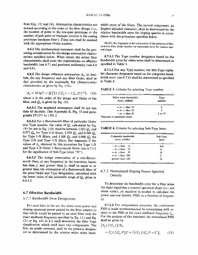
6.7.1.1 The Type number designator based on the bandwidth error for white noise shall be determined as specified in Table 3.
6.7.1.2 For any Type number, the Sub-Type alpha- bet character designator based on the composite band- width error (see 6.7.6) shall be determined as specified in Table 4.
TABLE 3. Criteria for selecting Type number.
White noise bandwidth error, millibel
= or < than 10 = or < than 25 =or < than 41
*depends on passband ripple.
Type number
0 1
2 or 3*
TABLE 4. Criteria for selecting Sub-Type letter.
Composite bandwidth error, millibel
=or <than 13 =or <than 25 = or <than 50 = or <than 100 greater than 100
Sub-Type letter
AA A B C D
6.7.2 Normalized Sloping Power Spectral Density
To determine the bandwidth error for a filter when the input signal has a nonzero spectrum slope (i.e., not white noise), an equation is needed to calculate the power spectral density, PSD, as a function of frequen- CY.
6.7.2.1 For computation purposes, the continuous PSD is made nondimensional. by normalizing with re- spect to the PSD at the exact midband frequency f,. For the purpose of this standard, the normalized PSD shall be given by
[&(f/fm )]/Sm
=C[(f/f,,“]C+ w[(f/fm)g+q, (11)
8 AMERICAN NATIONAL STANDARD
where S, (f /f, ) is the PSD of the signal at any fre- quency ratio f/f, ; g is the constant nondimensional slope of the normalized PSD function; S, is the PSD at midband frequency f = f, ; and C is a nondimen- sional constant equal to 2000.
NOTES: . . .
(1) If the normalized PSD in decibels is plotted versus the base 10 logarithm of the frequency ratio f/f,, then slope g equals the slope in decibels per octave divided by 10 lg( 2).
(2) The constant C is included in Eq. ( 11) to provide low-fre- quency and high-frequency asymptotes of constant normalized PSD to limit the calculated value of normalized wideband equivalent power (NWEP) passed by a bandpass filter when the input signal has a nonzero slope.
6.7.2.2 For octave-band filters, the NWEP trans-
mitted by a practical filter shall be determined for spectral slopes of g = - 5.0, 0.0, and + 3.0.
6.7.2.3 For fractional-octave-band filters, the NWEP transmitted by practical filter shall be deter- mined for values of g = - 12.0, 0.0, and + 10.0.
6.7.3 Normalized Equivalent Power of Noise Transmitted by an Ideal Filter
For a random noise signal having a spectrum slope g not equal to - 1 (for g= - 1, see Ref. Al), the NWEP, Wig/W,, transmitted by an ideal filter, with bandwidth designator b, shall be calculated from
wig/w, = [20.5(g+ ‘)b - 2-0.-g+ “b]/lg + I),
(12)
where Wig is the equivalent power (EP) transmitted by an ideal filter for input signal of spectral slope g and W,,, is the EP transmitted by the ideal filter at frequen- cy f = f, and equal to the product S,,, f, .
NOTES:
(1) Since the transmission of an ideal filter is unity between bandedges f, and f2 and is zero for all other frequencies, Eq. ( 12) may be obtained by the integral of [S, (f/f, ) l/S,,, = ( f/f, )g over the frequency range from f, and f2
(2) For octave-band filters, Wi,/W, = 0.707107 for g = 0 and 0.937500 for g = + 3 or - 5. For one-third-octave-band filters, Wi,/Wm = 0.231563 for g = 0 and 0.298453 forg = + 10 or - 12.
6.7.4 Normalized Equivalent Power of Noise Transmitted by a Realizable Filter
6.7.4.1 For a random noise signal, the total NWEP transmitted by a realizable filter shall be computed from
where [S, VG, ) ] EL, is given by Eq. ( 11) and IH, (f /f, I* is the measured or calculated squared magnitude transfer function of the filter under consi- deration and is equal to 10 _A ‘lo, where A is the at- tenuation in decibels.
6.7.4.2 The minimum attenuation ifi the passband shall be the reference for determining the attenuation characteristic as a function of frequency ratio (see 6.6.1 and 8.1.1).
6.7.4.3 For analog filters, the Type and Sub-Type designation shall be determined for the attenuation characteristic corresponding to the worst-case combi- nation of component tolerances. For a digital filter, the effect of the antialias filter shall be included. Where several different filters are combined to obtain one oc- tave band, the largest composite error shall be used to determine the Sub-Type designation.
6.7.4.4 The integral in Eq. ( 13) may be evaluated by any suitable method; numerical integration is rec- ommended. The range of values used for f /f, during an evaluation shall extend below and above 1.0 such that additional contributions to the value of the sum- mation do not change the calculated composite band- width error by more than 1 millibel to be consistent with the requirements of Table 4.
6.7.5 Determination of Filter Bandwidth Error
The bandwidth error, in millibels, shall be calculat- ed from
Eg = lWJQ[(w,/W,,,)/(wi,/Wm]
= 1000 lg( W&/W,). (14)
NOTE: The quantity IV,,, = S,,, f, that is used as a normalizing equivalent power in Eqs. (12) and ( 13) appears in both the numera- tor and denominator of the ratio in the middle term of Eq. (14). Hence, the actual value of the product is irrelevant to the determina- tion of the bandwidth error for any spectral slope g and may, if de- sired, be assigned an arbitrary value such as 1.0.
6.7.6 Composite Bandwidth Error
The composite bandwidth error EC to determine the Sub-Type designation for octave-band and fractional- octave-band filters, shall be determined from
Ec =31E,=oI + I&= p-51 + I&= +sl, (1%
Ec =Wg=ol + IEg= -121 + IEg= +,olt (15b)
respectively. The result shall be rounded to the nearest millibel and the Sub-Type determined in accordance with Table 4.
ANSI Sl .ll-1986
6.7.7 Filter Designation
To meet the requirements of this standard, a filter set or equivalent filtering system shall be marked to in- clude the applicable Order and Type designations. No filter set or equivalent shall be stated to be in accord with this standard unless its Order, Type, and Sub- Type designations are given. (Example: One-Third- Octave-Band Filter Set, Order 5, Type O-A, Extended Range, per ANSl Sl.ll-1986).
6.8 Passband Uniformity
The peak-to-valley ripple within the passband of each filter in the set, whether by design choice or effect of component tolerance, shall not exceed 10 millibels for Type O-X filters (see 7.2.2 for type O-X digital filters), 25 millibels for Type 1-X filters, or 50 milli- bels for Type 2-X filters. Filters having 60 to 200 milli- bels peak-to-valley ripple shall be designated as Type 3-X filters.
6.9 Variation of Reference Passband Attenuation
The reference passband attenuation, Eq. ( 17), of any filter band in a set shall not differ from the refer- ence passband attenuation of any other filter band in the set by more than 10 millibels for Type O-X, 30 mil- libels for Type l-X, 100 millibels for Type 2-X or 200 millibels for Type 3-X filters.
6.10 Removal of Filters From Circuit
If means are incorporated in the filter set to remove all filter bands from the circuit, the manufacturer shall explicitly state the frequency characteristics of the sub- stituted broadband circuit. Over a frequency range ex- tending 1 octave below and above the range of the fil- ter set, the frequency response of the broadband circuit shall have uniform (flat) response over the operating range and shall not droop below the midband flat re- sponse by more than 1 decibel at frequencies 1 octave below and above the analysis range of the filter set.
6.11 Terminating Impedances
6.11.1 The input and output terminating impe- dances necessary to ensure proper operation of filter sets shall be purely resistive. The necessary terminat- ing imbedances shall be explicitly labeled on the filter set.
6.11.2 Active filters shall be buffered, if necessary, to ensure that their operation is substantially indepen- dent of the terminating impedances between which they are connected.
6.12 Maximum Input Signal
The manufacturer shall state the maximum root- mean-square (rms) input wideband white or pink noise voltage and the maximum midband sinusoidal rms input voltage at which each filter in the filter set will meet the performance requirements of this stan- dard. Filter sets not dedicated to a specific instrument should be capable of accepting a sinusoidal rms input voltage of at least 1 volt.
6.13 linearity
For any steady input signal and for any input signal level within the specified operating range of the filter set, the transfer gain (output-to-input ratio) of each filter in a set shall not vary by more than 10 millibels for Type O-X and Type 1-X filters or 30 millibels for Type 2-X and Type 3-X filters.
6.14 Nonlinear or Harmonic Distortion
The manufacturer shall specify the total harmonic distortion in the output signal of a filter when a sinu- soidal signal of frequency f, at maximum rated vol- tage is applied to the input of any filter in the set. He shall also state how the distortion varies as the input voltage is reduced to zero.
6.15 Transient Response
When a sinusoidal signal of frequency f, is sudden- ly applied to the input of a filter, the maximum of the envelope of the signal voltage appearing at the output shall not exceed the steady state output voltage by more than a factor of 1.26 (2 dB) and the duration, in milliseconds, of the ringing, defined as the time re- quired for the output to settle to within 10 millibels of the steady state value, shall not exceed 2000 divided by the filter reference bandwidth in hertz [ Eq. (7) I.
6.16 Phase and Group Delay Response
See Appendix B for the phase and group delay characteristics of an exact reference-design Order 3 Butterworth filter. For filter designs different from the Order 3 Butterworth shown in Appendix B, the manu- facturer shall include the design-goal normalized phase and ,group delay response of. the filters in the In- struction Manual for the filter set.
6.17 Dynamic Range
The dynamic range of analog filters shall be not less than 80 decibels. If the dynamic range is less than 80
AMERICAN NATIONAL STANDARD
decibels, the manufacturer shall specify the value. (See 7.2.3 for minimum dynamic range requirement for di- gital filters.)
.’
6.18 Analysis of Nonstationary Signals
6.18.1 With the filter set or filter system incorporat- ed within a suitable measurement system that includes appropriate squaring and time-averaging capabilities (e.g., an integrating-averaging sound level meter or a fast-Fourier-transform analyzer), and with the voltage of the input signal constant at the manufacturer-speci- fied maximum sinusoidal input voltage (see 6.12)) for at least three filters in a filter set the difference between the time-period-average level L, of a contin- uous sinusoidal signal and the time-period-average lev- el L, of a burst of a sinusoidal signal that starts and stops at a zero crossing shall not differ from the theo- retical difference by more than 10, 30, 50, and 100 mil- libels for type 0, 1, 2, or 3 filters, respectively, but not to exceed the tolerance limits specified by the manu- facturer for the overall instrument accuracy. The com- plete measurement system shall be specified by the manufacturer in the Instruction Manual.
6.18.2 The theoretical difference, in millibels, between the two time-period-average levels of a con- tinuous sinusoidal signal and a sinusoidal tone burst of the same amplitude and frequency shall be determined from
L, -Lb = lOOOlg(T,,/T,), (16)
where T,, is the averaging time in seconds and Tb is the duration, in seconds, of the tone burst from the first to the last axis crossing.
6.18.3 The duration of the averaging time period T,, shall be at least 8 seconds for each test signal. For each filter tested, the length of the tone burst Nb shall be equal to 32 complete cycles at the nominal midband frequency in order to maintain a constant value of 7.41 for the product N,,B,.
6.18.4 The requirement in 6.18.1 shall apply to tone bursts occurring at any time during the duration of the total averaging time period, without use of internal triggering.
6.18.5 For filters intended for the audio-frequency range (see 6.1.1), the test frequencies shall include 125, 1000, and 8000 hertz. Manufacturers of filter sets intended for applications to other frequency ranges shall specify the test frequencies in the Instruction Manual.
6.19 Sensitivity to External Conditions
6.19.1 Temperature
The attenuation characteristics of the filter set shall conform to the applicable requirements of this stan- dard over the temperature range from - 10 “C to + 50 “C. If the influence of changes in ambient tem-
perature causes the tolerance limits on attenuation or effective bandwidth to be exceeded, conformance with this standard may be established by determining the influence of the environmental change by measure- ment to a precision of 10 millibels and making the in- formation available to the user of the filter set. The manufacturer shall indicate the ambient temperature limits and exposure time, which, if exceeded, may cause permanent damage to the filter set.
6.19.2 Humidity
The manufacturer shall state the range of relative humidity between which the filters will function cor- rectly together with the corresponding permissible ex- posure periods within the rated operating temperature range. At any temperature between - 10 “C and + 50 ‘C, the filters should operate indefinitely within the various tolerance limits over a relative humidity range extending from 10% to 90% without condensa- tion. If operation within the tolerance limits is not pos- sible over that combined range of temperature and hu- midity, the manufacturer shall state the amount and kind of degradation as a function of relative humidity, temperature, and exposure time.
6.19.3 Electromagnetic Fields
The effects of electromagnetic fields on the oper- ation of the filters shall be reduced as far as practical. The filters shall be tested in a magnetic field of strength 80 amperes per meter at 50 and 60 hertz and for the orientation which gives maximum response to the radiation. The manufacturer shall state the rms output voltage. For filters designed for use with a spe- cific type of instrument, e.g., a sound level meter, the output produced by the test field shall be given in terms of the output indication for each band affected.
6.19.4 Vibration
Portable filter sets should be designed and built to withstand transportation shock and vibration accelera- tions.
6.19.5 Sound
The rms voltage at the output of each filter in a set of filters for the audio-frequency range resulting from exposure to a sinusoidal sound field with a level of 110
ANSI Sl
decibels at the position of the filter set before its inser- tion and swept from 3 1.5 hertz to 8 kilohertz at a rate not greater than 0.1 octave per second shall be at least 80 decibels below the output voltage produced by a sinusoidal signal of maximum input voltage specified for the filter in accordance with 6.12.
7 SAMPLED DATA SYSTEMS
7.1 Analog Filters
Analog filters that are sampled in time are subject to all of the requirements of Sec. 6. Appendix D de-
scribes the general characteristics of one implementa-
tion of a sampled analog filter.
7.2 Digital Filters
7.2.1 Except as specified below, digital filters and
all numerically synthesized fractional-octave-band filters shall conform with all requirements of Sec. 6.
7.2.2 Antialias filters, analog and digital, shall pro- vide attenuation such that the sum of the guard filter attenuation plus the level of possible aliased spectra shall be equal to or greater than the dynamic range of the digital filter. Passband ripple in the guard filter may contribute to the passband ripple of the bandpass filter. For Type O-X filters, the total passband ripple specified in 6.8 may be increased to 15 millibels owing to this contribution.
7.2.3 The cutoff attenuation in the upper transition band of a digital bandpass filter shall not be increased by the attenuation of an antialias filter, either analog or digital, by an amount greater than that produced by placing the 3-dB-down frequency of such filter at the upper 40-dB attenuation frequency of the digital filter.
7.2.4 The minimum dynamic range of a digital filter shall be not less than 72 decibels.
7.2.5 The sampling rate of the analog-to-digital con- verter shall be sufficiently high not to affect signal components which are within the dynamic range and analysis band of the highest frequency filter.
7.2.6 The bilinear z transform [see Par. IV( 3 1) in Appendix E] is the preferred method for realizing a
1 l-1986 11
digital bandpass filter design from an analog prototype bandpass filter. If the bilinear transformation is used, then the inverse transformation (prewarping) shall be applied to the midband and bandedge frequencies of the prototype analog filter to maintain the applicable relationships specified in Sec. 6.
7.2.7 Deadband effect or limit cycle resulting from truncation error in recursive filter designs shall be ameliorated by appropriate means. See Par. V(9) in Appendix E.
8 METHOD OF TEST
Tests described in this section apply to analog, digi- tal, or numerically synthesized filters, as appropriate. When the digital data are available from a digital fil-
ter, before squaring and time averaging, all of the tests specified for an analog filter may be made by the addi- tion of a digital-to-analog converter and a post filter. In all cases, the manufacturer shall include in the In- struction Manual the procedures by which a user may verify the proper operation of the filters.
8.1 Attenuation Characteristic
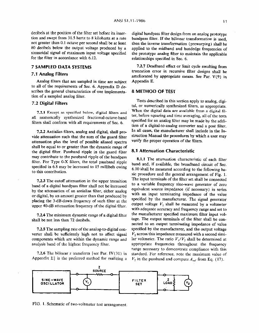
8.1.1 The attenuation characteristic of each filter band and, if available, the broadband circuit of Sec. 6.10 shall be measured according to the following ba- sic procedure and the general arrangement of Fig. 1. The input terminals of the filter set shall be connected to a variable frequency sine-wave generator of zero equivalent source impedance (if necessary) in series with an input terminating impedance of the value specified by the manufacturer. The signal generator output voltage V, shall be measured by a voltmeter with adequate accuracy and frequency range and set to the manufacturer specified maximum filter input vol- tage. The output terminals of the filter shall be con- nected to an output terminating impedance of value specified by the manufacturer, and the output voltage V2 across this impedance measured with a second simi- lar voltmeter. The ratio V,/V2 shall be determined at appropriate frequencies throughout the frequency range necessary to demonstrate compliance with this standard. For reference, note the maximum value of I’, in the passband and compute Aref from Eq. (17).
SINE-WAVE FILTER OSC I LLATOR SET
FIG. 1. Schematic of two-voltmeter test arrangement.
12 AMERICAN NATIONAL STANDARD
A,ef = 2o lg( vl/v*)min (17)
and the filter transmission loss A at any frequency is
A = 20 lg( V,/V,, -A,&. (18)
For a constant inpitt voltage V,, Eq. ( 18) reduces to
A = 20 lg( V,,,;V,,. (191
NOTE: The purpose of 8.1.1 is not to specify the only way in which filter characteristics and performance may be determined, but a basic way which does not require special purpose instruments. For the user of a sound level meter and fractional-octave-band analyzer who wishes to check his filter set, the obvious choice for the output measuring device is the sound level meter itself. For best accuracy, a digital display is preferred.
8.1.2 When the attenuation is being measured at frequencies below the lower bandedge frequency, a suitable technique shall be employed to remove the ef- fects of oscillator harmonics from the apparent re- sponse of the filter. A tuned voltmeter (wave analyz- er) shall not be used to remove those effects, since such a device at the output of the filter would simulta- neously remove any distortion or noise introduced by the filter set, which properly should be ascribed to analysis error of the filter set (see 6.14).
8.1.3 In establishing compliance with this standard, the attenuation characteristic of a filter shall be mea- sured using the maximum input signal voltage speci- fied by the manufacturer according to 6.12 and also at voltages that are smaller by factors of 0.32 and 0.032 (i.e., 10 decibels and 30 decibels below the maximum input level).
8.2 Dynamic Range
8.2.1 Analog Filters
With the filter set properly terminated at its input and output (see 6.11), and no other signal applied, measure the level of the time-averaged squared wide- band noise voltage appearing at the output of each fil- ter in the set. The difference between the maximum rated output level corresponding to the maximum rat- ed sinusoidal input (see 6.12) and the noise level is the dynamic range. The frequency range for the instru- ment used to measure the wideband output noise vol- tage shall be the same as for the measuring device with which the filter set would normally be used, e.g., the electronic circuits of a sound level meter.
8.2.2 Digital Filters
The dynamic range of digital filters shall be deter- mined from the overall system response from analog input to digital or analog output. The internal noise
floor of the filter shall be determined by applying a full scale sinusoidal signal at nominal midband frequency to one filter and measuring the level of the time-aver- aged squared output signal in another filter band suffi- ciently removed in frequency so that its attenuation at the frequency of the sinusoid is .equal to or greater’ than the expected dynamic range. The dynamic range, in decibels, is the difference in level between full scale input voltage and the noise floor.
8.3 Phase-Response Characteristic (Optional)
The typical phase response of a filter may be mea- sured in the same manner as the attenuation character- istic. A phase meter is preferred for these measure- ments, although an x-y oscilloscope displaying a Lissajous figure may be used. The reference phase shall be that of the signal generator output. All re- quirements on signal characteristics stated in Sec. 8.1 above apply to phase measurements. Since the phase shift of bandpass filters is zero at the midband frequen- cy and since the rate of change of phase with frequen- cy is large at this point, a sensitive means for determin- ing the actual midband frequency is provided by phase measurement (see Appendix B). The phase response may be determined at the same time the attenuation characteristic is measured.
APPENDIX A: PERFORMANCE OF BUTTERWORTH BANDPASS FILTERS
[This Appendix is not a part of American National Standard Speci- fication for Octave-Band and Fractional-Octave Band Analog and Digital Filters, Sl.ll-1986, but is included for information purposes only. ]
Al. Traditionally, filter bandwidths have been ex- pressed in terms of the half-power or the 3 dB-down frequencies of the filter. However, when random noise is analyzed, the power which is transmitted by a band- pass filter depends not only on the filter bandwidth but also on the steepness of the attenuation in the transi- tion band and the slope of the spectrum being ana- lyzed. For the 1966 version of this standard, the Writ- ing Group examined many representative sound
ANSiSl.ll-1986 13
spectra and found spectrum level slopes ranging from + 6 to - 21 decibels per octave. Since then, even
steeper spectrum level slopes have been found to occur in practice.
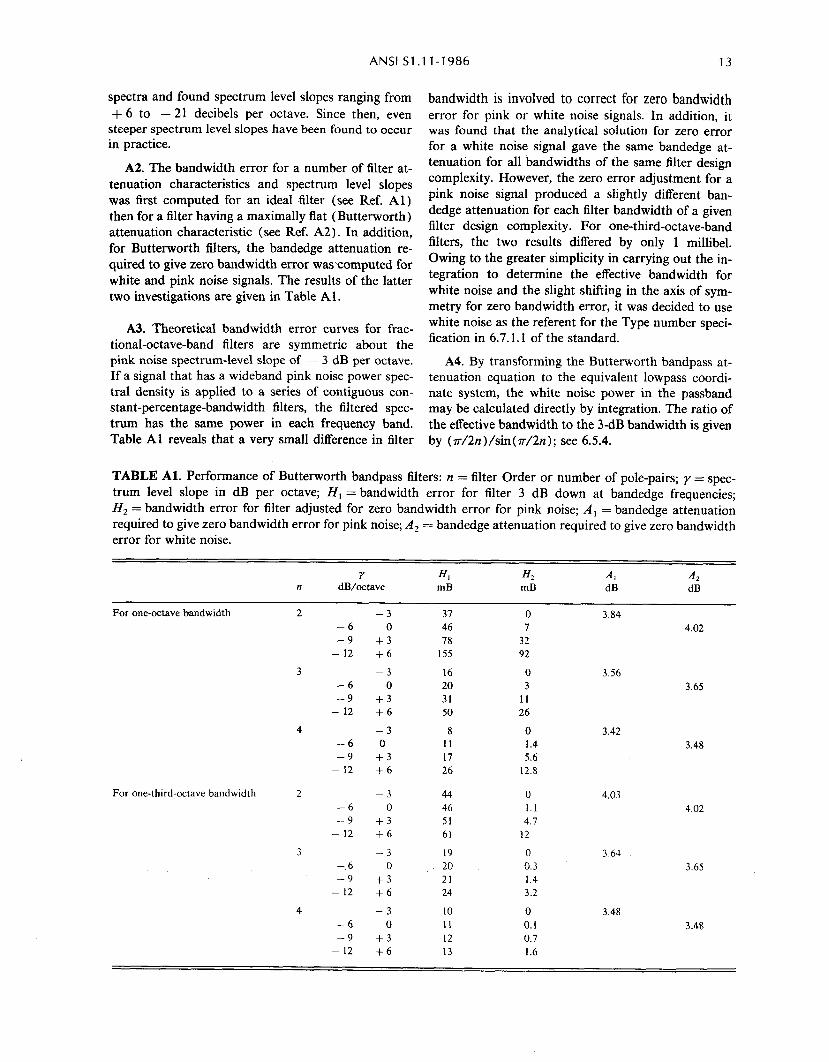
A2. The bandwidth error for a number of filter at- tenuation characteristics and spectrum level slopes was first computed for an ideal filter (see Ref. Al) then for a filter having a maximally flat (Butterworth) attenuation characteristic (see Ref. A2). In addition, for Butter-worth filters, the bandedge attenuation re- quired to give zero bandwidth error wascomputed for white and pink noise signals. The results of the latter two investigations are given in Table Al.
A3. Theoretical bandwidth error curves for frac- tional-octave-band filters are symmetric about the pink noise spectrum-level slope of - 3 dB per octave. If a signal that has a wideband pink noise power spec- tral density is applied to a series of contiguous con- stant-percentage-bandwidth filters, the filtered spec- trum has the same power in each frequency band. Table Al reveals that a very small difference in filter
bandwidth is involved to correct for zero bandwidth error for pink or white noise signals. In addition, it was found that the analytical solution for zero error for a white noise signal gave the same bandedge at- tenuation for all bandwidths of the same filter design complexity. However, the zero error adjustment for a pink noise signal produced a slightly different ban- dedge attenuation for each filter bandwidth of a given filter design complexity. For one-third-octave-band filters, the two results differed by only 1 millibel. Owing to the greater simplicity in carrying out the in- tegration to determine the effective bandwidth for white noise and the slight shifting in the axis of sym- metry for zero bandwidth error, it was decided to use white noise as the referent for the Type number speci- fication in 6.7.1.1 of the standard.
A4. By transforming the Butterworth bandpass at- tenuation equation to the equivalent lowpass coordi- nate system, the white noise power in the passband may be calculated directly by integration. The ratio of the effective bandwidth to the 3-dB bandwidth is given by (7r/2n)/sin(r/2n); see 6.5.4.
TABLE Al. Performance of Butterworth bandpass filters: n = filter Order or number of pole-pairs; y = spec- trum level slope in dB per octave; H, = bandwidth error for filter 3 dB down at bandedge frequencies; HZ = bandwidth error for filter adjusted for zero bandwidth error for pink noise; A, = bandedge attenuation required to give zero bandwidth error for pink noise; A, = bandedge attenuation required to give zero bandwidth error for white noise.
Y ff, ff2 ‘4, 4 n dB/octave mB mB dB dB
For one-octave bandwidth 2
For one-third-octave bandwidth 2
-6 -9
- 12
-6 -9
- 12
-6 -9
- 12
-6 -9
- 12
-.6 -9
- 12
-6 -9
- 12
-3 37 0 0 46 7
t3 78 32 +6 155 92
-3 16 0 0 20 3
+3 31 11 +6 50 26
-3 8 0 0 11 1.4
+3 17 5.6 i-6 26 12.8
-3 44 0 0 46 1.1
+3 51 4.1 +6 61 12
-3 0
+3 +6 -3
0 f3 +6
19 0 20 0.3 21 1.4 24 3.2
10 0 11 0.1 12 0.7 13 1.6
3.84 4.02
3.56 3.65
3.42 3.48
4.03 4.02
3.64 3.65
3.48 3.48
14 AMERICAN NATIONAL STANDARD
A5 A closed form integration of Eq. ( 13) for posi- function. The normalized equivalent noise power tive, even and unbounded spectrum slopes g was passed by an analog Butterworth fractional-octave- achieved by changes of variable (Ref. A3). However, band filter is given by removal of the asymptotes introduced by the constant C in Eq. ( 11) may cause the resulting calculated val- ues of E, tp be slightly larger than those found by nu- merical integration of Eq. (13) in conjunction, with
[A,, (@I y 1’2Qd)fk(T’2n) , We
use of Eq. ( 11) for the normalized spectrum slope Wi*
= d, k$ 0 sm[ (2k + l)?r/2n]
(Al)
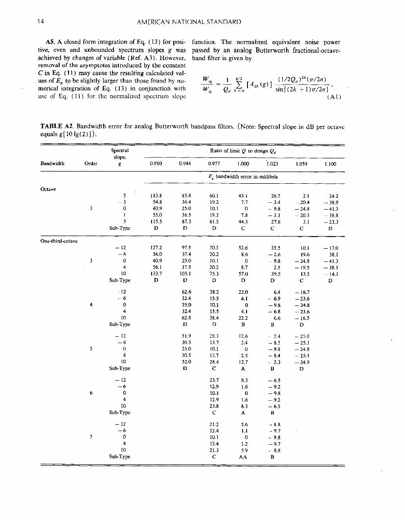
TABLE A2. Bandwidth error for analog Butter-worth bandpass filters. {Note: Spectral slope in dB per octave equals g[ 10 lg(2)]}.
Bandwidth Order
Spectral slope,
g 0.910 0.944
Ratio of limit Q to design Q,
0.977 1.ooo 1.023 1.059 1.100
E, bandwidth error in millibels
Octave
3
-5 113.8 85.8 60.1 43.1 26.7 2.1 - 24.2 -3 54.8 36.4 19.2 7.7 - 3.4 - 20.4 - 38.9
0 40.9 25.0 10.1 0 - 9.8 - 24.8 - 41.3 1 55.0 36.5 19.3 7.8 - 3.3 - 20.3 - 38.8 3 115.5 87.3 61.5 44.3 27.8 3.1 - 23.3
Sub-Type D D D C C C D
One-third-octave - 12
-6 3 0
4 10
Sub-Type
52.6 35.5 8.6 - 2.6
0 - 9.8 8.7 - 2.5
57.0 39.5 D D
- 12 -6
0 4
10 Sub-Type
22.0 6.4 4.1 - 6.9
0 - 9.8 4.1 - 6.8
22.2 6.6 B B
- 12 -6
5 0 4
10 Sub-Type
127.2 97.5 70.5 56.0 37.4 20.2 40.9 25.0 10.1 56.1 37.5 20.2
133.7 103.1 75.3 D D D
62.6 38.2 32.4 15.5 25.0 10.1 32.4 15.5 62.8 38.4 D D
51.9 28.3 30.5 13.7 25.0 10.1 30.5 13.7 52.0 28.4 D C
23.7 12.9 10.1 12.9 23.8
C
12.6 - 2.4 - 25.0 2.4 - 8.5 - 25.1
0 - 9.8 - 24.8 2.5 - 8.4 - 25.1
12.7 - 2.3 - 24.9 A B D
- 12 -6
6 0 4
10 Sub-Type
8.3 - 6.5 1.6 - 9.2
0 - 9.8 1.6 - 9.2 8.3 - 6.5 A B
- 12 21.2 5.6 - 8.8 -6 12.4 1.1 - 9.7
7 0 10.1 0 - 9.8 4 12.4 1.2 - 9.1
10 21.3 5.9 - 8.8 Sub-Type C AA B
10.1 - 17.0 - 19.6 - 38.1 - 24.8 - 41.3 - 19.5 - 38.1
13.5 - 14.1 C D
- 16.7 - 23.6 - 24.8 - 23.6 - 16.5
D
ANSlSl.ll-1986 15
where
l&(g) = [(g/2) +kl! 22k/C[(g/2) --kl! 2k!) (A21
for g even and = or < zero. See 6.5.4 for values of
Qe A6. Table A2 presents the bandwidth errors for the
limit conditions specified for Butterworth bandwidth quotient in 6.6.3.2 for Order 3 octave-band and for one-third-octave-band filters of Order 3 through 7. The resulting Sub-Type designation in accordance with 6.7.6 and Table 4 is also given for each case.
A7. Close empirical approximations for the band- width error of Butterworth filters using the values of Qd given by Eq. (9) were determined by curve fitting procedures.. For both octave-band and one-third-oc- tave-band filters, the approximate bandwidth error is given by
E,-m*(g + 2)’ (-43) for negative values of spectrum slope g.
For octave-band filters of Order n = or > 2,
m=4.5/&[ 1 + (l/n) + (2/n’)]). (A4)
For one-third-octave-band filters of Order n = or > 3,
m1:1.5/&[1+ (l/n) + (l/n’)l). (A5)
AB. References
A’L. W. Sepmeyer, “Bandwidth error of symmetrical bandpass filters used for analysis of noise and vibration,” J. Acoust. Sot. Am. 34, 1653 (1962).
AzL. W. Sepmeyer, “On bandwidth error of Butterworth bandpass filters,” J. Acoust. Sot. Am. 35, 404 (1963).
A3 J. Kalb (private communication).
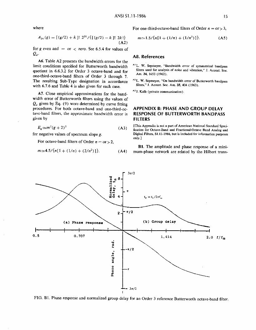
APPENDIX B: PHASE AND GROUP DELAY RESPONSE OF BUTTERWORTH BANDPASS FILTERS [This Appendix is not a part of American National Standard Speci- fication for Octave-Band and Fractional-Octave Band Analog and Digital Filters, Sl.ll-1986, but is included for information purposes only.]
Bl. The amplitude and phase response of a mini- mum-phase network are related by the Hilbert trans-
(a) Phase response (b) Group delay
I I 1 1 I L I I 1
0.5 0.707 2.0
FIG. Bl. Phase response and normalized group delay for an Order 3 reference Butterworth octave-band filter.
16 AMERICAN NATIONAL STANDARD
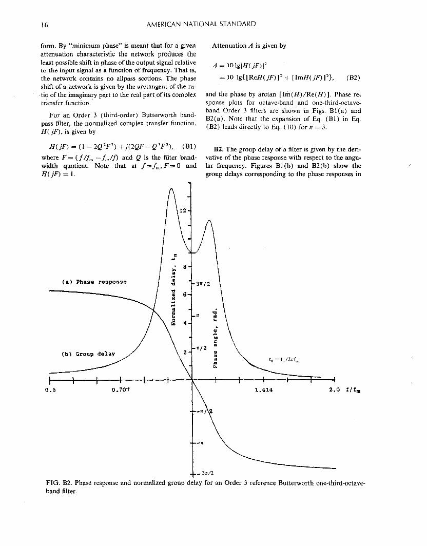
form. By “minimum phase” is meant that for a given attenuation characteristic the network produces the least possible shift in phase of the output signal relative to the input signal as a function of frequency. That is, the network contains no allpass sections. The phase shift of a network is given by the arctangent of the ra- tio of the imaginary part to the real part of its complex transfer function.
For an Order 3 (third-order) Butterworth band- pass filter, the normalized complex transfer function, H( jF), is given by
H(jF) = (1 - 2Q2F2) +j(2QF- Q3F3), (Bl)
where F = ( f/f, -f,/’ and Q is the filter band- width quotient. Note that at f = f,, F = 0 and H(jF) = 1.
q
(a) Phase response
Attenuation A is given by
A = 10 lg)H(jF) 12
= 10 IgCtRd(jF)12 + tImH(jF)l*~, (B2)
and the phase by arctan [Im(H)/Re(H)]. Phase re- sponse plots for octave-band and one-third-octave- band Order 3 filters are shown in Figs. Bl (a) and B2(a). Note that the expansion of Eq. (Bl) in Eq. (B2) leads directly to Eq. ( 10) for n = 3.
B2. The group delay of a filter is given by the deri- vative of the phase response with respect to the angu- lar frequency. Figures Bl(b) and B2(b) show the group delays corresponding to the phase responses in
+- 3?r/2
FIG. B2. Phase response and normalized group delay for an Order 3 reference Butterworth one-third-octave- band filter.
ANSlSl.ll-1986 17
Figs. Bl(a) and B2(a). Note that the group delay is APPENDIX C: ATTENUATION FOR ORDER 3 not constant in the passband of the filter, nor is it sym- OCTAVE-BAND AND ONE-THIRD-OCTAVE- metric with respect to midband frequency. In Figs. BAND FILTERS Bl (a) and Bl (b) the group delays are presented as normalized time delays t, , which are related to actual [This Appendix is not a part of American National Standard Speci-
group delay time td by t, = ( td ) (2?rf, ). fication for Octave-Band and Fractional-Octave Band Analog and Digital Filters, St.1 t-1986, but is included for information purposes only .]
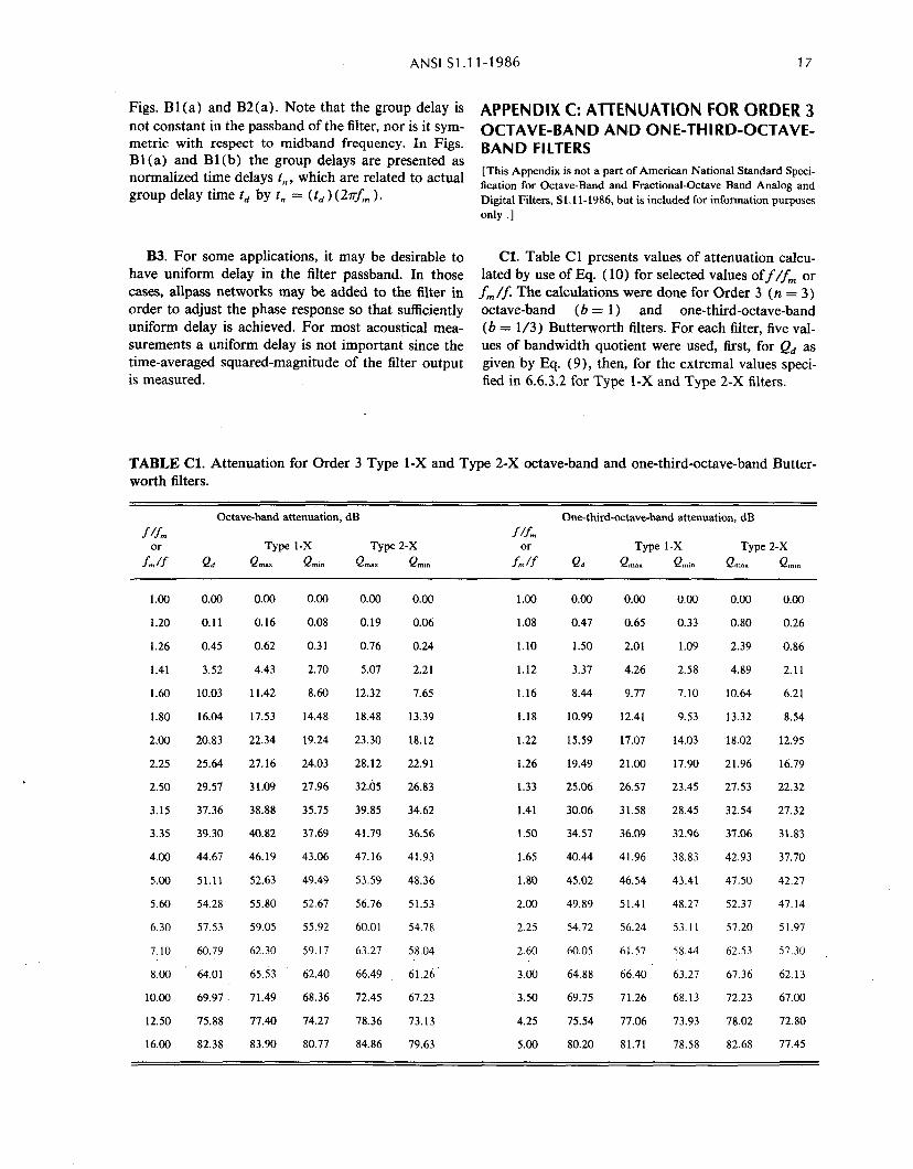
B3. For some applications, it may be desirable to Cl. Table Cl presents values of attenuation calcu- have uniform delay in the filter passband. In those lated by use of Eq. ( 10) for selected values off/f, or cases, allpass networks may be added to the filter in f,/’ The calculations were done for Order 3 (n = 3) order to adjust the phase response so that sufficiently octave-band (b = 1) and one-third-octave-band uniform delay is achieved. For most acoustical mea- (b = l/3) Butterworth filters. For each filter, five val- surements a uniform delay is not important since the ues of bandwidth quotient were used, first, for Qd as time-averaged squared-magnitude of the filter output given by Eq. (9), then, for the extremal values speci- is measured. fied in 6.6.3.2 for Type 1-X and Type 2-X filters.
TABLE Cl. Attenuation for Order 3 Type 1-X and Type 2-X octave-band and one-third-octave-band Butter- worth filters.
Octave-band attenuation, dB One-third-octave-band attenuation, dB
f/f, f/f, Type 1-X Type 2-X
f,";r Q‘, Qmx Qmin Qmx Qmi. Type 1-X Type 2-X
fi?f Qd Qmx Qmi, Qm Qmin
1.00
1.20
1.26
1.41
1.60
1.80
2.00
2.25
2.50
3.15
3.35
4.00
5.00
5.60
6.30
7.10
8.00
10.00
12.50
16.00
0.00
0.11
0.45
3.52
10.03
16.04
20.83
25.64
29.57
37.36
39.30
44.67
51.11
54.28
57.53
60.79
64.01
69.91
75.88
82.38
0.00 0.00 0.00
0.16 0.08 0.19
0.62 0.31 0.76
4.43 2.70 5.07
11.42 8.60 12.32
17.53 14.48 18.48
22.34 19.24 23.30
27.16 24.03 28.12
31.09 27.96 32.65
38.88 35.75 39.85
40.82 37.69 41.79
46.19 43.06 47.16
52.63 49.49 53.59
55.80 52.67 56.76
59.05 55.92 60.01
62.30 59.17 63.27
65.53 62.40 66.49
71.49 68.36 72.45
77.40 74.27 78.36
83.90 80.77 84.86
0.00
0.06
0.24
2.21
7.65
13.39
18.12
22.91
26.83
34.62
36.56
41.93
48.36
51.53
54.78
58.04
61.26
67.23
73.13
79.63
1.00 0.00 0.00 0.00 0.00 0.00
1.08 0.47 0.65 0.33 0.80 0.26
1.10 1.50 2.01 1.09 2.39 0.86
1.12 3.37 4.26 2.58 4.89 2.11
1.16 8.44 9.77 7.10 10.64 6.21
1.18 10.99 12.41 9.53 13.32 8.54
1.22 15.59 17.07 14.03 18.02 12.95
1.26 19.49 21.00 17.90 21.96 16.79
1.33 25.06 26.57 23.45 27.53 22.32
1.41 30.06 31.58 28.45 32.54 27.32
1.50 34.57 36.09 32.96 37.06 31.83
1.65 40.44 41.96 38.83 42.93 37.70
1.80 45.02 46.54 43.41 47.50 42.27
2.00 49.89 51.41 48.27 52.37 47.14
2.25 54.72 56.24 53.11 57.20 5 1.97
2.60 60.05 61.57 58.44 62.53 57.30
3.00 64.88 66.40 63.27 67.36 62.13
3.50 69.75 71.26 68.13 72.23 67.00
4.25 75.54 77.06 73.93 78.02 72.80
5.00 80.20 81.71 78.58 82.68 77.45
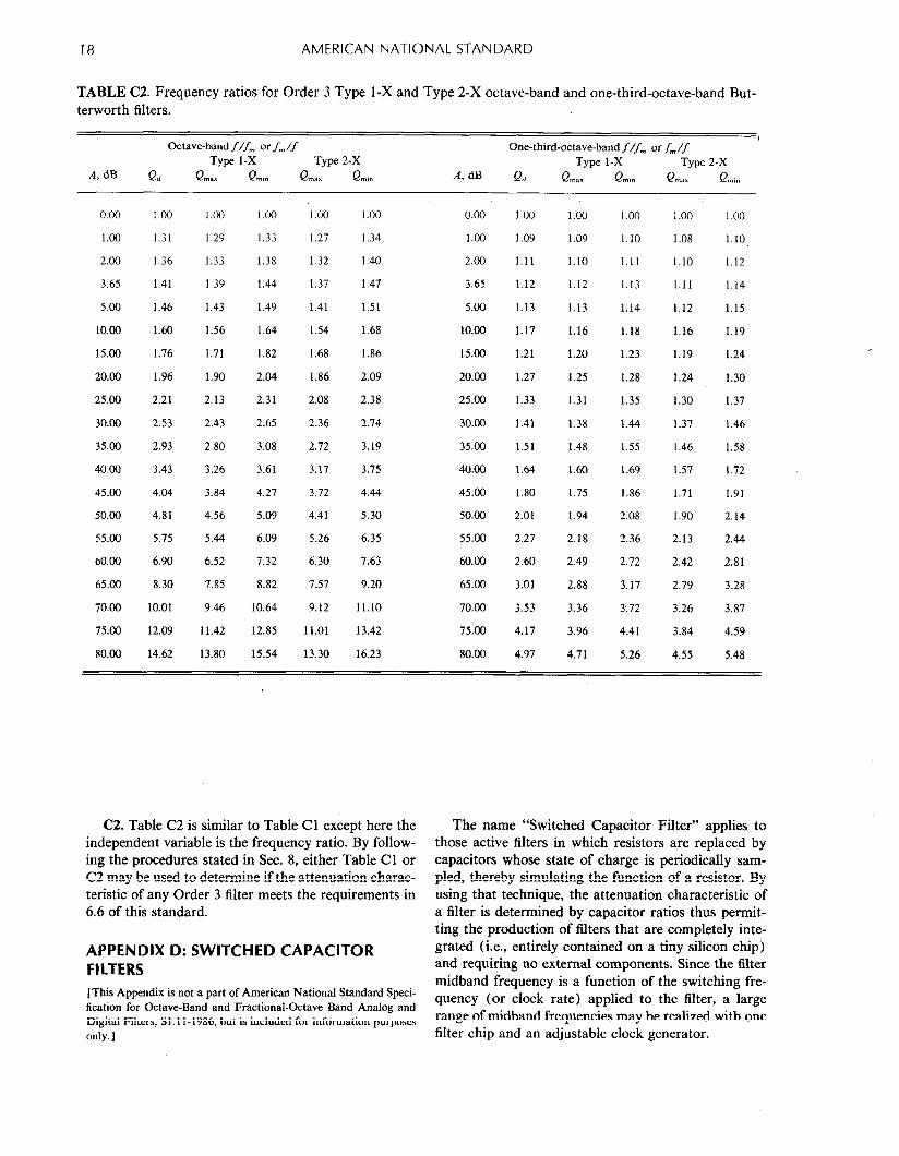
18 AMERICAN NATIONAL STANDARD
TABLE C2. Frequency ratios for Order 3 Type 1-X and Type 2-X octave-band and one-third-octave-band But- ter-worth filters.
0.00 l.oil 1.00 1.00 1.00 l.O!l 0.00 1.00 1.00 1.00 1.00 1.00
1.00 1.31 1.29 1.33 1.27 1.34 1.00 1.09 1.09 1.10 1.08 1.10
2.00 1.36 1.33 1.38 1.32 1.40 2.00 1.11 1.10 1.11 1.10 1.12
3.65 1.41 1.39 1.44 1.37 1.47 3.65 1.12 1.12 1.13 1.11 1.14
5.00 1.46 1.43 1.49 1.41 1.51 5.00 1.13 1.13 1.14 1.12 1.15
10.00 1.60 1.56 1.64 1.54 1.68 10.00 1.17 1.16 1.18 1.16 1.19
15.00 1.76 1.71 1.82 1.68 1.86 15.00 1.21 1.20 1.23 1.19 1.24
20.00 1.96 1.90 2.04 1.86 2.09 20.00 1.27 1.25 1.28 1.24 1.30
25.00 2.21 2.13 2.31 2.08 2.38 25.00 1.33 1.31 1.35 1.30 1.37
30.00 2.53 2.43 2.65 2.36 2.74 30.00 1.41 1.38 1.44 1.37 1.46
35.ccl 2.93 2.80 3.08 2.72 3.19 35.00 1.51 1.48 1.55 1.46 1.58
40.00 3.43 3.26 3.61 3.17 3.75 40.00 1.64 1.60 1.69 1.57 1.72
45.cm 4.04 3.84 4.27 3.72 4.44 45.00 1.80 1.75 1.86 1.71 1.91
50.00 4.81 4.56 5.09 4.41 5.30 50.00 2.01 1.94 2.08 1.90 2.14
55.00 5.75 5.44 6.09 5.26 6.35 55.00 2.21 2.18 2.36 2.13 2.44
60.00 6.90 6.52 7.32 6.30 7.63 60.00 2.60 2.49 2.72 2.42 2.81
65.00 8.30 7.85 8.82 7.57 9.20 65.00 3.01 2.88 3.17 2.79 3.28
70.00 10.01 9.46 10.64 9.12 11.10 70.00 3.53 3.36 3.72 3.26 3.87
75.00 12.09 11.42 12.85 11.01 13.42 75.00 4.17 3.96 4.41 3.84 4.59
80.00 14.62 13.80 15.54 13.30 16.23 80.00 4.97 4.71 5.26 4.55 5.48
I
Octave-band f/f, or f,/f One-third-octave-band//f, orf,/f Type 1-X Type 2-X Type 1-X Type 2-X
A, dB Qd Q max Qm. Qm,x Qmi. A, dB Qc, Pm, Qmm Qmx Pm,.
C2. Table C2 is similar to Table Cl except here the independent variable is the frequency ratio. By follow- ing the procedures stated in Sec. 8, either Table Cl or C2 may be used to determine if the attenuation charac- teristic of any Order 3 filter meets the requirements in 6.6 of this standard.
APPENDIX D: SWITCHED CAPACITOR FILTERS [This Appendix is not a part of American National Standard Speci- fication for Octave-Band and Fractional-Octave Band Analog and Digital Filters, Sl.ll-1986, but is included for information purposes only.]
The name “Switched Capacitor Filter” applies to those active filters in which resistors are replaced by capacitors whose state of charge is periodically sam- pled, thereby simulating the function of a resistor. By using that technique, the attenuation characteristic of a filter is determined by capacitor ratios thus permit- ting the production of filters that are completely inte- grated (i.e., entirely contained on a tiny silicon chip) and requiring no external components. Since the filter midband frequency is a function of the switching fre- quency (or clock rate) applied to the filter, a large range of midband frequencies may be realized with one filter chip and an adjustable clock generator.
ANSI Sl.ll-1986 19
APPENDIX E versus discrete time are often made. Although they are
[This Appendix is not a part of American National Standard Speci- often used interchangeably, different meanings should
fication for Octave-Band and Fractional-Octave Band Analog and be attributed to the two sets of terms.
Digital Filters, Sl.ll-1986, but is included for information purposes 2) The term analog generally describes a waveform only. ] that is continuous in time (or any other appropriate
independent variable) and that belongs to a class that
Terminology in Digital can take on a continuous range of amplitude values. Examples of nnnlog wunveforms or unalog signals are those
Signal Processing derived from acoustic sources. Such signals are repre- sented mathematically as functions of a continuous
LAWRENCE R. RABINER, JAMES W. COOLEY, variable. The functions sin (wl) and the step function
HOWARD D. HELMS, LELAND B. JACKSON, azc-t(t) are examples of common mathematical functions
JAMES F. KAISER, CHARLES M. RADER, that could describe “analog signals.” The use of the RONALD W. SCHAFER, KENNETH STEIGLITZ, term “analog” in this context appears to stem from the and CLIFFORD J. WEINSTEIN field of analog computation, where a current or voltage
Abstract-The committee on Digital Signal Processing of the waveform serves as a physical ‘analog of some variable
IEEE Group on Audio and EIectroacoustics has undertaken the in a differential equation.
project of recommending terminology for use in papers and texts on 3) The term confinuozrs time implies that only the digital signal processing. The reasons for this project are twofold. independent variable necessarily takes on a continuous First, the meanings of many terms that are commonly used differ range of values. In theory the amplitude may, but need from, one author to another. Second, there are many terms that one would lie to have defined for which no standard term currently
not, be restricted to a finite or countable infinite set of
exists. It is the purpose of this paper to propose terminology which we values (i.e., the amplitude may be quantized). There-
feel is self-consistent, and which is in reasonably good agreement fore, analog waveforms are continuous-time waveforms with current practices. An alphabetic index of terms is included at with continuous amplitude. In practice, however, “con- the end of the paper. tinuous-time waveforms” and “analog waveforms” are
Introduction equivalent. Since most signal processing problems have
As an aid to cjassifying the different types of terms nothing to do with analogs as such, the use of the term analog waveform is often ambiguous at the least and
to be defined, we have placed each term in one of the may in fact be misleading. Thus, the term continuous- following groups: time waveform is preferable.
1) Introductory Terms---General Definitions 4) ‘Discrete time implies that time (the independent 2) Discrete Systems-Block Diagram Terminology variable) is quantized. That is, discrete-time signals are 3) Relations Between Discrete and Continuous defined only for discrete values of the independent vari-
Signals able. Such signals are represented mathematically as 4) Theory and Design of Digital Filters 5) Finite Word Length Effects-A/D, D/A Con-
seqzlences of numbers. Those discrete-time signals that take on a continuum of values are referred to as sampled-
version 6) Discrete Fourier Transforms and the FFT
data signals.
7) Discrete Convolution and Spectrum Analysis. 5) The term digital implies that both time and ampli-
In the above mentioned sections of this paper we will be &de are quantized. Thus a digital system is one in which
discussing terminology related to the processing of one- signals are represented as sequences of numbers which take on only a finite set of values. Thus one uses dig&z/
dimensional signals. For convenience, we will assume when discussing actual physical realizations (as hard- that this dimension is time-although the definitions apply equally well to any single dimension.
ware or programs) of discrete-time signal processing sys- tems, whereas the t&m discrete time is a better modifier
I. Introductory Terms-General Definitions when considering mathematical abstractions of such systems in which the effects of amplitude quantization
1) In discussing waveform processing problems, the are ignored. A digital signal or digital waveform is a se-
distinctions analog versus digital and continuous time quence produced, for example, by digital circuitry or by an analog-to-digital converter which is sampling a con-
Manuscript received August 1, 1972. L. R. Rabiner. J. F. Kaiser, and R. W. Schafer are with Bell
tinuous-time waveform. In digital signal processing
Telephone Laboratories, Inc., Murra Hill, N. J. 07974. J. W. Cooley is with the IBM ‘I! J. Watson Research Center,
these terms are commonly shortened to signal or wave-
Yorktown Height?, N..Y. 10598. form. Sometimes the term signal is restricted to being a
H. D. Helms IS wth Bell Telephone Laboratories, Inc., \\‘hip- desirable component of a sequence instead of being used pany,.N. J. 07981.
L. B.. Jackson is with Rockland Systems Corporation, West interchangeably with waveform. Noise is either defined
” Nyack, N. Y. 10994. as a) an undesirable’ component of, a sequence, or b) .a. C. AI. Rader and C. J. LVeinsteiu we with M.I.T. Lincoln Lab-
oratory, Lexington, Mass. 02173. (Operated with support from the sequence of random variables.
U. S. Air Force.) 6) (Digifal) simulation is the exact or approximate K. Steiglitz is with Princeton University, Princeton, N. J. 08540. representation of a given system (discrete or contin-
a.1972 IEEE. Reprinted with permission from IEEE Transactions on Audio and Electroacoustics Vol. AU-20, No. 5, December 1972.
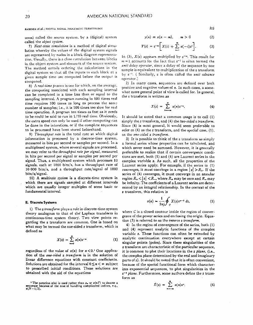
20 AMERICAN NATIONAL STANDARD
RAB~NER el al.: DIGITAL SIGXAL PROCESSISG TER>IISOLOGV
uous) called the source system, by a (digital) system called the object sysfem.
7) Next-slate simulation is a method of digital simu- lation whereby the values of the digital system signals are represented by nodes in a block diagram representa- tion. Usually, there is a close correlation between i,lWl;s in the object system and elemerlts of the source system. The method entails ordering the calculations in the digital system so that all the inputs to each block at a given sample time are computed before the output is computed.
8) A real-time ~tocess is one for which, on the average, the computing associated with each sampling interval can be completed in a time 1~s than or equal to the sampling interval. A program running in 100 times real time requires 100 times as long to process the Sam: number of samples; i.e., it is 100 times too slow for real time operation. A program ten times as fast as it needs to be could be said to run in l/10 real time. Obviously, the extra speed can only be llsed if other computing can be done in the interstices, or if the complete sequences to be processed have been stored beforehand.
9) Throughput rute is the total rate at which digital information is processed by a discrete-time system, measured in bits per second or samples per second. In a multiplexed system, where several signals are processed, we may refer to the throughput rate per signal, measured in bits per second per signal or samples per second per signal. Thus, a multiplexed system which processes 10 signals, each at 1000 bits/s, has a throughput rate of 10 000 bits/s, and a throughput rate/signal of 1000 bits/s/signal.
10) A m&rate syskm is a discrete-time system in which there are signals sampled at different intervals which are usually integer multiples of some basic or fundamental interval.
II. Discrete Systems
1) The .z transform plays a role in discrete-time system theory analogous to that of th6 Laplace transform in continuous-time system theory. Two view points re- garding the z transform are common. One is based on what may be termed the one-sided z transform, which is defined as
X(z) = 2 z(n)&* (1) n-0
regardless of the value of x(n) for n<O.l One applica- tion of the one-sided z transform is in the solution of linear difference equations with constant coefficients. Solutions are obtained for the interval O<n< 00 subject to prescribed initial conditions. These solutions are obtained with the aid of the equations
’ The notation x(n) is used rather than xn or ~$27 to denote a sequence because of the ease of handling complicated indices, e.g., 0-l/2).
j2j
y(n) = x(n - m), ??t>b (2)
Y(z) = z- [X(z) + g +azi]. (3)
In (3), X(i) appears multiplied by zPm. This result for m = 1 accounts for the fact that 5-I is often termed the unif delay operator, since a delay of the sequence by one sample is equivalent to multiplication of the z transform by z-l. ( Similarly, z is often called the unif advance operator.)
2) In many cases, sequences are defined over both positive and negative values of n. In such cases, a some- what more genera1 point of view is called for. In general, the z transform is written as
X(z) = 2 x(n)z-n. (4) n-c4
It should be noted that a common usage is to call (1) simply the z transform, and (4) the two-sided z transform. Since (4) is most general, it would seem preferable to refer to (4) as the z transform, and the special case, (l), as the one-sided z transform.
3) It is possible to think of the z transform as simply a formal series whose properties can be tabulated, and which never need be summed. However, it is generally preferable to realize that if certain convergence condi- tions are met, both (1) and (4) are Laurent series in the complex variable z. As such, all the properties of the Laurent series apply. For example, if the series in (1) converges, it must con<erge in a region 1 z] > R+. If the series of (4) converges, it must converge in an annular region R+ < 1 z[ <R-, where R+ may be zero and R- may be infinity. The coefficients of a Laurent series are deter- mined by an integral relationship. In the context of the z transform, this relation is
1 x(n) = -
f 2rj c X(z)z”-’ dz,
where C is a closed contour inside the region of conver- gence of the power series and enclosing the origin. Equa- tion (5) is referred to as the inverse z transform.
4) In the region of convergence of the series, both (1) and (4) represent analytic functions of the complex variable z. These functions can often be extended by analytic continuation everywhere except at certain singular points (poles). Since these singularities of the z transform are characteristic of the particular sequence, it is common to.pIot their locations in the z plane, (i.e., the complex plane determined by the real and imaginary parts of e). It should be noted that it is often convenient, because of the special functional form which character- izes exponential sequences, to plot singularities in the z-1 plane. Furthermore, some authors define the z trans- form as
X(z) = 2 x(n)zn. (6) n-4
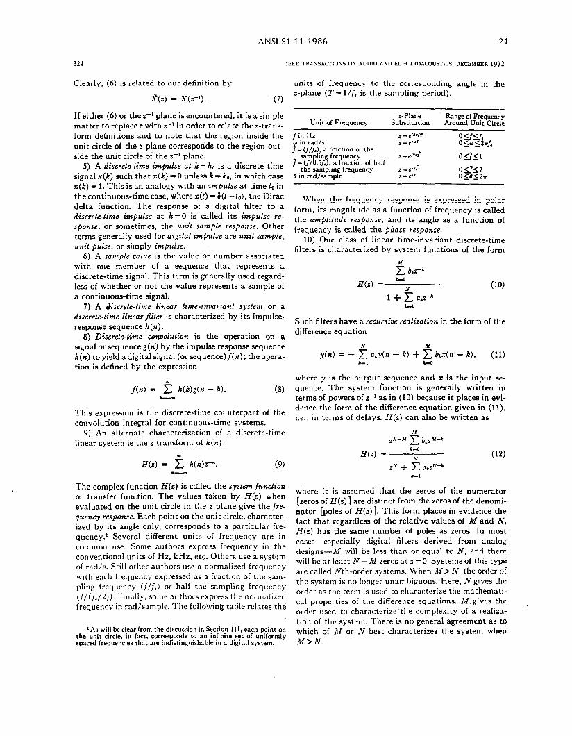
ANSlSl.ll-1986 21
321 ,EEE TRANSACTIONS OS AUDIO AND ELECTROACOUSTICS, DECEMBER 1972
Clearly, (6) is related to our definition by
X(z) = X(2-‘). (7)
If either (6) or the z-i plane is encountered, it is a simple matter to replace z with z-t in order to relate the s-trans- form definitions and to note that the region inside the unit circle of the z plane corresponds to the region out- side the unit circle of the z-r plane.
5) A discrele-time impulse at k = ko is a discrete-time signal r(k) such that x(k) = 0 unless k = ko, in which case x(k) = I. This is an analogy with an impulse at time lo in the continuous-time case, where x(l) = 8(t --lo), the Dirac delta function. The response of a digital filter to a discrete-time impulse at k = 0 is called its impulse re- sponse, or sometimes, the unil sample response. Other terms generally used for digital impulse are unit sample, unil pulse, or simply impulse.
6) A sample value is the value or number associated with one member of a sequence that represents a discrete-time signal. This term is generally used regard- less of whether or not the value represents a sample of a continuous-time signal.
7) A d.iscrete-lime linear time-invariant system or a discrete-time linear jilter is characterized by its impulse- response sequence h(n) .
8) Discrefa-time convolution is the operation on a signal or sequence g(n) by the impulse response sequence h(n) to yield a digital signal (or sequence)f(n) ; the opera- tion is defined by the expression
This expression is the discrete-time counterpart of the convolution integral for continuous-time systems.
9) An alternate characterization of a discrete-time linear system is the 2 transform of h(n):
H(z) = 2 k(n)z-“. (9) I-W
The complex function H(z) is called the system ficndion or transfer function. The values taken by H(z) when evaluated on the unit circle in the z plane give the fre- quency response. Each point on the unit circle, character- ized by its angle only, corresponds to a particular fre- quency.* Several different units of frequency are in common use. Some authors express frequency in the conventional units of Hz, kHz, etc. Others use a system of rad/s. Still other authors use a normalized frequency with each frequency expressed as a fraction of the sam- pling frequency (f/j,) or half the sampling frequency cf/cf./2)). Finally, some authors express the normalized frequency in radfsample. The following table relates the
*As will be clear from the discussion in Section I I I, each point on the unit circle, in fact. corresponds to an illfinite set of uniformly spaced frequencies that are indistinguishable in P digital system.
units of frequency to the corresponding angle in the z-plane (T= l/f. is the sampling period).
Unit of Frequency z-Plane
Substitution Range of Frequency Around Unit Circle
fin Hz z =&IT 0 in r,ad/s e = eivr
0 If If.
f- (f/f,), a fraction of the Olwl2rf.
sampling frequency z = @.i i- (f/O.Sf.). a fraction of half
Wfll
the sampling frequency z = ei*i 19 in rad/sample
OljlS z=& 0<852r
When the frequency response is expressed in polar form, its magnitude as a function of frequency is called the amplitude response, and its angle as a function of frequency is called the phase response.
10) One class of linear time-invariant discrete-time filters is characterized by system functions of the form
5 brz-”
a(z) = ^4, - 1 f c akz-”
t-1
Such filters have a reczrrsive realizaliolt in the form of the difference equation
y(n) = - 5 aky(n - k) + 2 brx(n - k), (11) k-l k-0
where y is the output sequence and x is the input se- quence. The system function is generally written in terms of powers of 2-l as in (10) because it places in evi- dence the form of the difference equation given in (ll), i.e., in terms of delays. H(z) can also be written as
Z‘N--M 2 btz”-”
H(z) = *;O rv + c akzNvk
k-l
(12)
where it is assumed that the zeros of the numerator [zeros of H(z)] are distinct from the zeros of the denomi- nator [poles of H(z)]. This form places in evidence the fact that regardless of the relative values of M and N, H(z) has the same number of poles as zeros. In most cases-especially digital filters derived from analog designs--M will be less than or equal to N, and there will be at least N-M zeros at z = 0. Systems of this type are called Nth-order systems. When M> N, the order of the system is no longer unambiguous. Here, N gives the order as the term is used to characterize the mathemati- cal properties of the difference equations. M.gives the order used to characterize‘the complexity of a realiza- tion of the system. There is no general agreement as to which of dl or N best characterizes the system when M>N.
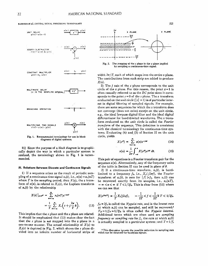
22 AMERICAN NATIONAL STANDARD
RAEINER C; (11.: DIGITAL SIGHAL PROCESSING TER~lINOLOGY 325
“NIT DELAY y(n) =r(n-0 YzP
ADDER/ SUBTRACTOR r(nl=xinl ;ty(n)
CONSTANT MULTIPLIER y(n) = k, r(n)
x(nl kl y(n)
MULTIRATE DELAY (r IS THE SAMPLING
BRANC”lNG OPERATION f -
MULTIPLYING TWO SIGNALS r(nl= *(n). y(n1
Fig. 1. Recommended terminology for use in block diagrams of digital systems.
11) Since the purpose of a block diagram is to graphi- cally depict the way in which a particular system is realized, the terminology shown in Fig. 1 is recom- mended.
III. Relations Between Discrete and Continuous Signals
1) If a sequence arises as the result of periodic sam- pling of a continuous-time signal xc(t), i.e., x(n) =r,(nT) where T is the sampIing period, then X(z), the z trans- form of x(n), is related to X,(s), the Laplace transform of x,(t) by the relationship
=- i kgx.(,+jfk). (13)
This implies that the s plane and the z plane are related. It should be emphasized that (13) makes clear the fact that the s plane is not mapped into the e plane in a one-to-one manner. The actual. relationship of X(z) to X,(S) is depicted in Fig. 2, which shows the s plane di-
X(eJW~) = ; X&274, --&<f<+Tif T< 1/2j0.
f~ = 2f0 is called the Nyquist rate, and is the lowest rate at which x.(t) can be sampled, and still be recovered.5 TN = l/fnr = 1/2f0 is often called the Nyquist interval. Additional terms which are often used are sampling frequency or san(rpZing rate for f., the rate at which x&) is actually sampled in a particular system; and T= l/f.
vided into an infinite number of horizontal strips oE 1 This discussion ignores the possible reduction in sampling rate
which can be obtained for bandpass signals.
jw
J 5 PLANE L PLANE
------
t 37 ------ ---e----7
I
Fig. 2. The mapping of the s plane to the L plane implied by sampling a continuous-time signal.
width 27r/T, each of which maps into the entire z pIane. The contributions from each strip are added to produce X(z).
2) The j axis of the s plane corresponds to the unit circle of the z plane. For this reason, the point z = 1 is often casually referred to as the DC point since it corre- sponds to the point s = 0 of the s plane. The z transform evaluated on the unit circle (I Z] = 1) is of particular inter- est in digital filtering of sampled signals. For example, there are some sequences for which the z transform does not converge (does not exist) except on the unit circle, e.g., the idea1 Iowpass digital filter and the idea1 digital differentiator for band-limited waveforms. The z trans- form evaluated on the unit circle is called the Fourier transform of the sequence. This definition is consistent with the classical terminology for continuous-time sys- tems. Evaluating (4) and. (5) of Section II on the unit circle, yields
X(es) = 2 z(n)6-” a-
(14)
This pair of equations is a Fourier transform pair for the sequence x(n). Alternatively, any of the frequency units of the table in Section II can be used in place of 6.
3) If a continuous-time waveform, x,(l), is band- limited to a frequency f~, i.e., X.(j27rfl, the Fourier transform of x,(l), is zero for If] >fo, then r,(l) can be recovered exactly from its samples, i.e., x.(nT), - CO <n < 00 if T< 1/2f,. This is clear from (13) where we can see that
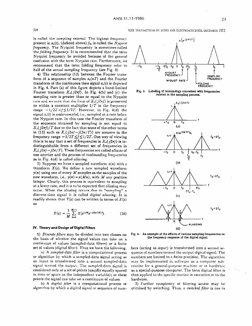
ANSI Sl .l l-l 986 23
326 TEEE TRASSACTlOSS OS KDIO MD ELECTKOACOUSTICS, DECEYBER 1972
is called the sampling inlewal. The highest frequent? present in x,(t), (defined above) fo, is called the Nyqrlist frequency. The h’yquist frequency is sometimes called the folding frequency. It is recommended that the term Nyquist frequency be avoided because of the general confusion with the term Nyquist rate. Furthermore, \ve recommend that the term folding frequency refer to half of the actual sampling frequency (see Fig. 3).
4) The relationship (13) between the Fourier trans- form of a sequence of samples x,(nT) and the Fourier transform of the continuous time signal ~~(1) is depicted in Fig. 4. Part (a) of this figure depicts a band-limited Fourier transform X,(jZrrf). In Fig. 4(b) and (c) the sampling rate is greater than or equal to the Nyquist rate and we note that the form of X,(j27$) is preserved to within a constant multiplier l/T in the frequency range -1/2T<f<1/2T. However, in Fig. 4(d) the signal xc(t) is zrnde~snmpled, i.e., sampled at a rate below the Nyquist rate. In this case the Fourier transform of the sequence obtained by sampling .is not equal to X,(j27rf)/T due to the fact that some of the other terms in (13) such as X,(j2s-f-j(lzr/T)) are nonzero in the frequency range - 1/2Tsf5 1/2T. One way of viewing this is to say that a set of frequencies in X,(j27$) is in- distinguishable from a different set of frequencies in X,( j2rf- jfrr/ T). These frequencies are called aliases of one another and the process of confounding frequencies as in Fig. 4(d) is called aliusing.
5) Suppose we have a sampled waveform x(n) with J transform X(z). We define a new sampled waveform r(n) using one of every M samples as the samples of the new waveform, i.e., r(n) =n(Mn), with M any positive integer. Clearly, this process is equivalent to sampling at a lower rate, and it is to be expected that aliasing may occur. When the aliasing occurs due to “sampling” a discrete-time signal it is called digital aliming. It is
readily shown that Y(z) can be written in terms of X(z) as
IV. Theory and Design of Digital Filters
1) Discrete filters may be divided into two classes on the basis of whether the signal values can take on a continuum of values (sampled-data filters) or a finite set of values (digital filter). Thus we have the following.
a) A sampled-data jilter is a computational process or algorithm by which a sampled-data signal acting as an input is transformed into a second sampled-data signal termed the output. The sampled-data signal is considered only at a set of points (usually equally spaced in time or space as the independent variable); at these points the signal can take on a continuum of values.
b) A digital jilter is a computational process or algorithm bv which a digital sicnal or seouence of nun,-
g s s 00 0 0
T 5 fS
2 NY’XJIST FREOUENCY f
1 t
t f SAMPLING
NYOUIST RATE FREQUENCY
FOLDING FREOUENCY
Fig. 3. Labeling of terminology concerned with frequencies related to the sampling process.
, X,(j27rfI
AL. -fo 0 fo
(4
0)
m tf..2fo
-to 0 to I 3fo Pfo=fs
(c)
/qp f fSC2f0
L ALIASING
(a
Fig. 4. An example of the effects of various sampling frequencies on the frequency response of the digital signal.
bers (acting as input) is transformed into a second se- quence of numbers termed the output digital signal. The numbers are limited to a finite precision. The algorithm may be implemented in software as a computer sul)- routine for a general-purpose .machine or in hardware as.a specialipurpose computer. The term digitat.filter is then applied to the specific routine in execution or to the hardware.
2) Further complexity of filtering action may bch ol)tnined bv switchine. Thus. a switched filter is one in
2, , -0 ,. .-
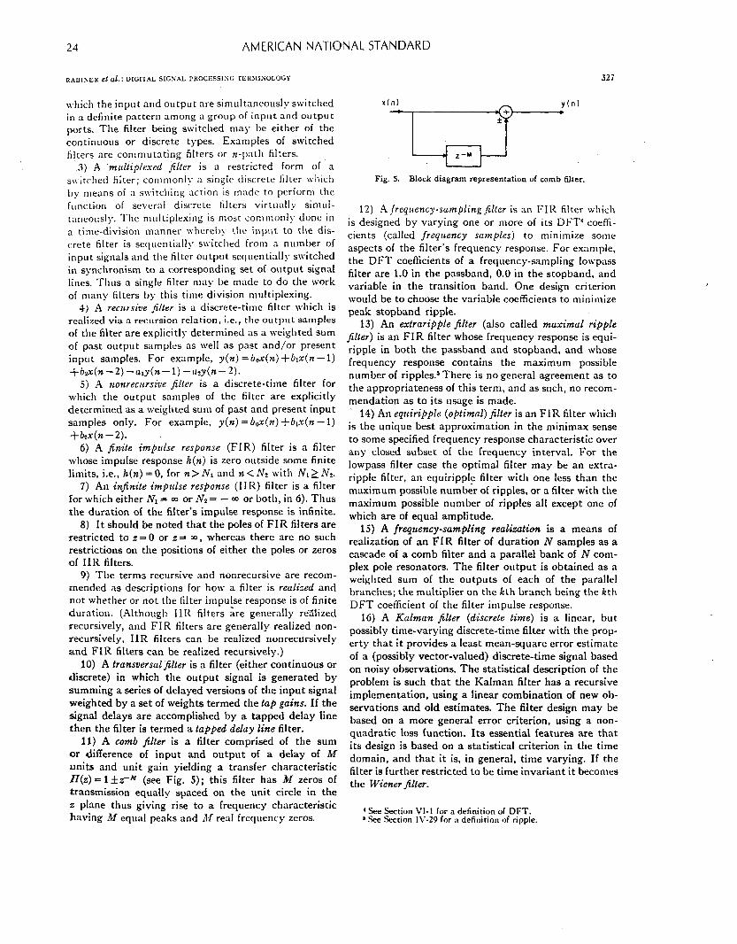
AMERICAN NATIONAL STANDARD
\vhich the input and output are simultaneously switched in a definite pattern among a group of input and output ports. The filter being switched may be either of the continuous or discrete types. Examples of switched filters are commutating filters or n-path filters.
3) A .mrrliip/exed filter is a restricted form of a su-itclled filter; commonly a single discrete tiller \vhich by means of a switching action is made to perform the ftlnction of several discrete titters virtually simul- t:~neously. The multiplexing is most commonly done in a time-division manner \\-hereby the input to the dis- crete filter is sequentially switched from a number of input signals and the filter output sequentialI>. switched in synchronism to a corresponding set of output signal lines. Thus a single filter may be made to do the work of many filters by this time division multiplexing.
4) A reclrrsive jilter is a discrete-time filler which is realized via a recursion relation, i.e., the output samples of the filter are explicitly determined as a weighted sum of past output samples as well as past and/or present input samples. For example, y(n) =6&(n) +&x(n - 1) +bzx(n-2)-aaly(n-l)--cl?y(n-2).
5) A nonreczrrsive jilter is a discrete-time filter for which the output samples of the filter are explicitly determined as a weighted sum of past and present input samples only. For example, y(n) = b&(n) +bl?c(n - 1) $-b&Z - 2).
6) A finite imp&e response (FIR) filter is a filter whose impulse response k(n) is zero outside some finite limits, i.e., k(n) =O, for n> N1 and n<N2 with NL> N2.
7) An injnite imp&e response (I I R) filter is a filter for which either No = 0~ or Nz = - 03 or both, in 6). Thus the duration of the filter’s impulse response is infinite.
8) It should be noted that the poles of FIR filters are restricted to z = 0 or I = m , whereas there are no such restrictions on the positions of either the poles or zeros of IIR filters.
9) The terma recursive and nonrecursive are recom- mended as descriptions for how a filter is realized and not whether or not the filter impulse response is of finite duration. (Although IIR filters are generally re‘9lized recursively, and FIR filters are generally realized non- recursively, IIR filters can be realized nonrecursively and FIR filters can be realized recursively.)
10) A transversalfilter is a filter (either continuous or discrete) in which the output signal is generated by summing a series of delayed versions of the input signal weighted by a set of weights termed the tap gains. If the signal delays are accomplished by a tapped delay line then the filter is termed a tapped delay line filter.
11) A comb jilter is a filter comprised of the sum or difference of input and output of a delay of M units and unit gain yielding a transfer characteristic H(z) = 1 fz-M (see Fig. 5); this filter has M zeros of transmission equally spaced on the unit circle in the 2 plane thus giving rise to a frequency characteristic having M equal peaks and M real frequency zeros.
(nl
Fig. 5. Block diagram representation of comb filter.
12) A jreqllency-sumpling filler is an FIR filter which is designed by varying one or more of its DFT’ coeffi- cients (called freqrrency samples) to minimize some aspects of the filter’s frequency response. For example, the DFT coefficients of a frequency-sampling lowpass filter are 1.0 in the passband, 0.0 in the stopband, and variabte in the transition band. One design criterion would be to choose the variable coefficients to minimize peak stopband ripple.
13) An extraripple jilter (also called muximal ripple jlter) is an FIR filter whose frequency response is equi- ripple in both the passband and stopband, and whose frequency response contains the maximum possible number of ripples5 There is no general agreement as to the appropriateness of this term, and as such, no recom- mendation as to its usage is made.
14) An eqzcirippEe (optimal) jilter is an FIR filter which is the unique best approximation in the minimax sense to some specified frequency response characteristic over any closed subset of the frequency interval. For the lowpass filter case the optimal filter may be an extra- ripple filter, an equiripple filter with one less than the maximum possible numb& of ripples, or a filter with the maximum possible number of ripples all except one of which are of equal amplitude.
1.5) A frequency-sampling realization is a means of realization of an FIR filter of duration N samples as a cascade of a comb filter and a parallel bank of N com- plex pole resonators. The filter output is obtained as a weighted sum of the outputs of each of the parallel branches; the multiplier on the kth branch being the kth DFT coefficient of the filter impulse response.
16) A Kulman filter (discrete time) is a linear, but possibly time-varying discrete-time filter with the prop- erty that it provides a least mean-square error estimate of a (possibly vector-valued) discrete-time signal based on noisy observations. The statistical description of the problem is such that the Kalman filter has a recursive implementation, using a linear combination of new ob- servations and old estimates. The filter design may be based on a more general error criterion, using a non- quadratic loss function. Its essential features are that its design is based on a statistical criterion in the time domain, and that it is, in general, time varying. If the filter is further restricted to be time invariant it becomes the Wiener fitter.
4 See Section VI-1 for a definition of DFT. ‘See Section IV-29 for n definition of ripple.
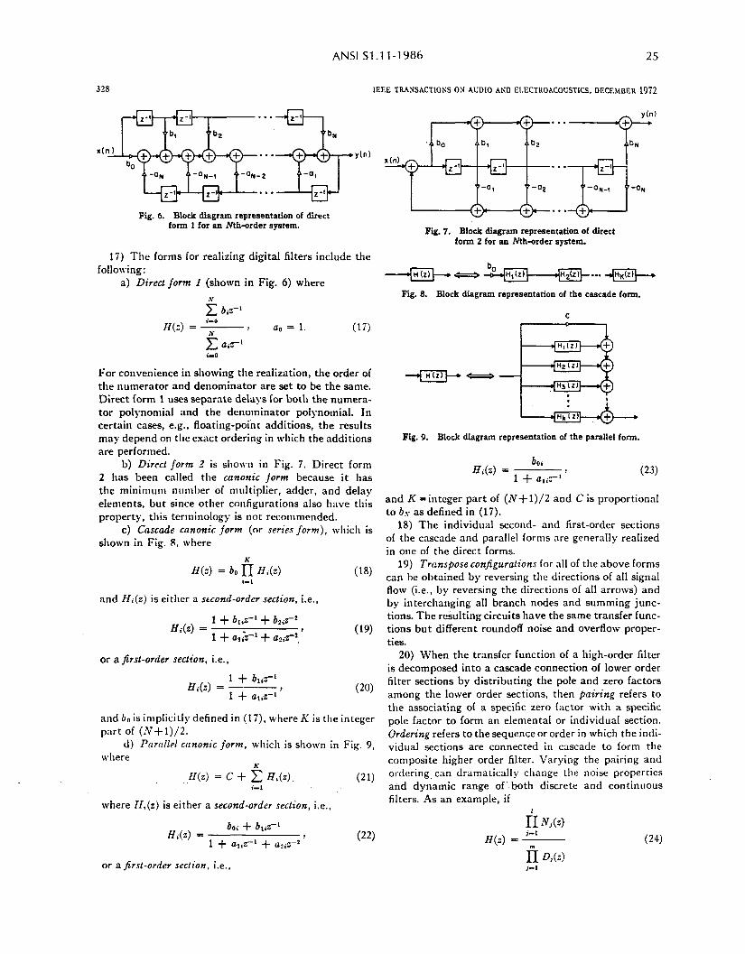
b,
ANSI Sl .l l-l 986 25
IEEE TRAXSACTIOZiS ON AUDIO AKD ELECTROACOUSTICS, DECEMBER 1072
Fig. 6. Block diagram representation of direct form 1 for an Nth-order system.
17) The forms for realizing digital filters include the following:
a) Direct form 1 (shown in Fig. 6) where
5 biz-’
H(z) = +--, a0 = 1. (13
For convenience in showing the realization, the order of the numerator and denominator are set to be the same. Direct form 1 uses separate delays for both the numera- tor polynomial and the denominator polynomial. In certain cases, e.g., floating-point additions, the results may depend on the exact ordering in which the additions are performed.
b) Direct form d is sho~11 in Fig. 7. Direct form 2 has been called the cunonic form because it has the minimum number of multiplier, adder, and delay elements, but since other configurations also have this property, this terminology is not recommended.
c) Cnscude canonic form (or series form), which is shown in Fig. 8, where
H(z) = b,, fi H,(z) i-l
(18)
and Hi(z) is either a stcond-order section, i.e.,
Hi(Z) = 1 + b,iZ-’ + b2iz-’
1 + Urii-r + aTiT’, ’ (19)
or a first-order section, i.e.,
Hi(z) = 1 + b,jz-’ --t 1 + a*iz-1
and bo is implicitly defined in (17), where K is the integer part of (N+1)/2.
d) Parallel canonic form, which is shown in Fig. 9, where
H(z) = c + 5 H,(z) (21) i- 1
where H,(z) is either a second-order section, i.e.,
Hi(z) = bo< + bliz-’
1 + a,,z-’ + ai,z-2 ’
or a first-order secfion, i.e.,
(22)
I y...-+$)
Fig. 7. Block diagram representation of direct form 2 for an Nth-order system.
Fig. 8. Block diagram representation of the cascade form.
Fig. 9. Block diagram representation of the parallel form.
H,(z) = bOi
1 + U*iZ-’ ’
and K = integer part of (N+1)/2 and C is proportional to b.~ as defined in (17).
18) The individual second- and first-order sections of the cascade and parallel forms are generally realized in one of the direct forms.
19) Transpose configurafions for all of the above forms can be obtained by reversing the directions of all signal flow (i.e., by reversing the directions of all arrows) and by interchanging all branch nodes and summing junc- tions. The resulting circuits have the same transfer func- tions but different roundoff noise and overflow proper- ties.
20) When the transfer function of a high-order filter is decomposed into a cascade connection of lower order filter sections by distributing the pole and zero factors among the lower order sections, then p&ring refers to the associating of a specific zero factor with a specific pole factor to form an elemental or individual section. Ordering refers to the sequence or order in which the indi- vidual sections are connected in cascade to form the composite higher order filter. Varying the pairing and ordering. can dramatically change the noise properties and dynamic range of’ both discrete and continuous filters. As an example, if
I? NAZI H(z) = Lp-- (24)
JiI D,(z) PI
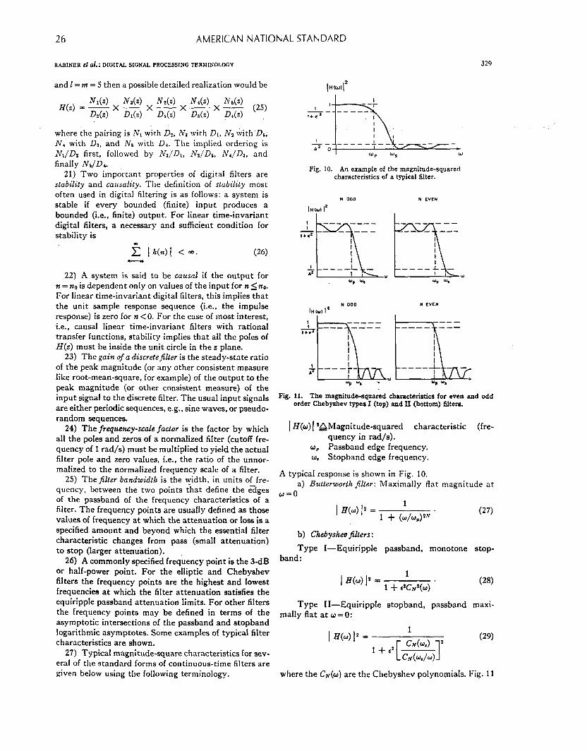
26 AMERICAN NATIONAL STANDARD
RABINER et cd.: DIGITAL SIGNAL PROCESSING TERMINOLOGY
and I = m = 5 then a possible detailed realization would be
Ndz) H(z) = - fV&)
D&l X-
N4z) Ddz)
X- D&)
where the pairing is Nr with Dz,-Na with DI, NS with’D6, N, with Da, and Ns with Da. The implied ordering is Nl/Dn first, followed by NJDI, NJD,, NI/D3, and finally Nb/D4.
21) Two important properties of digitai filters are stability and causality. The definition of stability most often used in digital filtering is as follows: a system is stable if every bounded (finite) input produces a bounded (i.e., finite) output. For linear time-invariant digital filters, a necessary and sufficient condition for stability is
22) A system is said to be causal if the output for tr = no is dependent only on values of the input for n_<no. For linear time-invariant digital filters, this implies that the unit sample response sequence (i.e., the impulse response) is zero for n <O. For the case of most interest, i.e., causal linear time-invariant filters with rational transfer functions, stability implies that all the poles of H(z) must be inside the unit circle in the z plane.
23) The gain of a discretefilter is the steady-state ratio of the peak magnitude (or any other consistent measure like root-mean-square, for example) of the output to the peak magnitude (or other consistent measure) of the input signal to the discrete filter. The usual input signals are either periodic sequences, e.g., sine waves, or pseudo- random sequences.
24) The frequency-scale facfor is the factor by which all the poles and zeros of a normalized filter (cutoff fre- quency of 1 rad/s) must be multiplied to yield the actual filter pole and zero values, i.e., the ratio of the unnor- malized to the normalized frequency scale of a filter.
25) The fitter bandwidth is the width, in units of fre- quency, between the two points that define the edges of the passband of the frequency characteristics of a filter. The frequency points are usually defined as those values of frequency at which the attenuation or loss is a specified amount and beyond which the essential filter characteristic changes from pass (small attenuation) to stop (larger attenuation).
26) A commonly specified frequency point is the 3-dB or half-power point. For the elliptic and Chebyshev filters the frequency points are the highest and lowest frequencies at which the filter attenuation satisfies the equiripple passband attenuation limits. For other filters the frequency points may be defined in terms of the asymptotic intersections of the passband and stopband logarithmic asymptotes. Some examples of typical filter characteristics are shown.
27) Typical magnitude-square characteristics for sev- eral of the standard forms of continuous-time filters are given below using the following terminology.
329
Fig. 10. An example of the magnitude-squared characteristics of a typical filter.
Fig. 11. The magnitude-squared characteristics for even and odd order Chebyshev types.1 (top) and II (bottom) filters.
1 H(w) 1 *&Iagnitude-squared characteristic (fre- quency in rad/s).
o, Passband edge frequency. w. Stopband edge frequency.
A typical response is shown in Fig. 10. a) BulterworUr filler: Maximally flat magnitude at
w=o
’ Hb) I2 = 1 + (:,u,,2‘v . b) Chebyshevfilters:
Type I-Equiripple passband, monotone stop- band :
w9
Type II-Equiripple stopband, passband maxi- mally flat at w = 0:
1 H(w) I* = (29)
where the CM(W) are the Chebyshev polynomials. Fig. 11
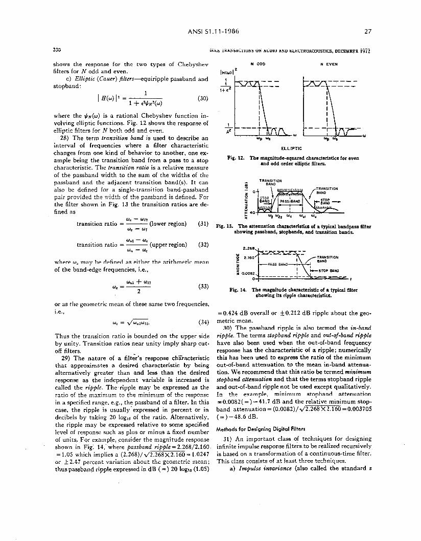
ANSI Sl .l l-1986 27
330 IEEE TRANSACTIONS ON AUDIO AND ELECTROACOUSTICS, DECEMBER 19’12
shows the response for the two types of Chebyshev filters for N odd and even.
c) Elliptic (Cauer) jilters-equiripple passband and stopband:
p7(u)12= l 1 + &‘N*(u)
(30)
where the #N(W) is a rational Chebyshev function in- volving elliptic functions. Fig. 12 shows the response of elliptic filters for N both odd and even.
28) The term transition band is used to describe an interval of frequencies where a filter characteristic changes from one kind of behavior to another, one ex- ample being the transition band from a pass to a stop characteristic. The transifion ratio is a relative measure of the passband width to the sum of the widths of the passband and the adjacent transition band(s). It can also be defined for a single-transition band-passband pair provided the width of the passband is defined. For the filter shown in Fig. 13 the transition ratios are de- fined as
transition ratio We - WI1
= - (lower region) (31) 0.5 - Wt
transition ratio = Wul - WC - (upper region) (32) a” - Qb
where ws may be defined as either the arithmetic mean of the band-edge frequencies, i.e.,
w&l + WI? w, =
2 (33)
or as the geometric mean of these same two frequencies, i.e.,
WC = ~/w”lWl2. (34)
Thus the transition ratio is bounded on the upper side by unity. Transition ratios near unity imply sharp cut- off filters.
29) The nature of a filt&‘s response chzracteristic that approximates a desired characteristic by being alternatively greater than and less than the desired response as the independent variable is increased is called the ripple. The ripple may be expressed as the ratio of the maximum to the minimum of the response in a specified range, e.g., the passband of a filter. In this case, the ripple is usually‘expressed in percent or in decibels by taking 20 log10 of the ratio. Alternatively, the ripple may be expressed relative to some specified level of response such as phs or minus a fixed number of units. For example, consider the magnitude response shown in -Fig: 14,“where passband ripple = 2.268/2.160 = 1.05 which implies a (2.268)/d2.268X2.160 = 1.0247 or +2.47 percent variation about the geometric mean; thus passbapd ripple expressed in dB (=) 20 log,, (1.05)
N EVEN
ELLIPTIC
Fig. 12. The magnitude-squared characteristics for even and odd order elliptic filters.
Fig. 13. The attenuation characteristics of a typical bandpass filter showing passband, stopbands, snd transition bands.
Fig. 14. The magnitude characteristic of a typical titer showing its ripple characteristics.
=0.424 dB overall or kO.212 dB ripple about the geo- metric mean.
30) The passband ripple is also termed the in-band ripple. The terms stopband ripple and out-of-band ripple have also been used when the out-of-band frequency response has the characteristic of a ripple; numerically this has been used to express the ratio of the minimum out-of-band attenuation to the mean in-band attenua- tion. We recommend that this ratio be termed minimum stopband uttenuafion and that the terms stopband ripple and out-of-band ripple not be used except qualitatively. In the example, minimum stopband attenuation =0.0082( =) -41.7 dB and the relative minimum stop- band attenuation = (0.0082)/d/2.268 X2.160 =0.003705 (=) -48.6 dB.
Methods for Designing Digital Filters
31) An important class of techniques for designing infinite impulse response filte;s.to be realized recursively is based on a transformation of a continuous-time filter. This class consists of at least three techniques.
a) Impulse invariance (also called the standard z
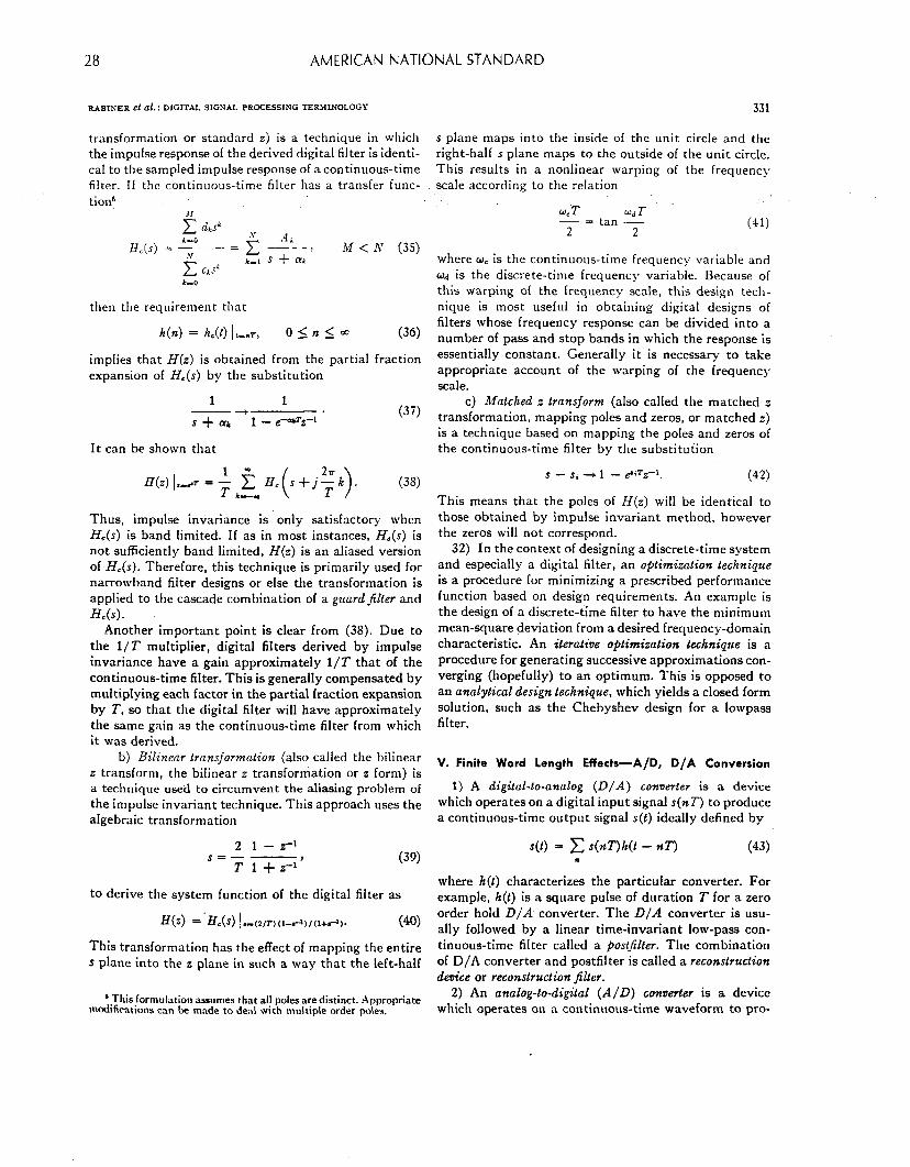
28 AMERICAN NATIONAL STANDARD
UBINER et d.: DIGITAL SIGNAL PROCESSING TERMINOLOGY
transformation or standard z) is a technique in which the impulse response of the derived digital filter is identi- cal to the sampled impulse response of a continuous-time filter. If the continuous-time filter has a transfer func- tions
k-0
then the requirement that
h(n) = h,(f) (t4, O<PZlm (36)
implies that H(z) is obtained from the partial fraction expansion of HJs) by the substitution
(37)
It can be shown that
1 k--o. \ 1 /
Thus, impulse invariance is only satisfactory when H,(S) is band limited. If as in most instances, H,(S) is not sufficiently band Iimited, H(z) is an aliased version of H,(s). Therefore, this technique is primarily used for narrowband filter designs or else the transformation is applied to the cascade combination of a guard jilter and H,(s).
Another important point is clear from (38). Due to the l/T multiplier, digital fiIters derived by impulse invariance have a gain approximately l/T that of the continuous-time filter. This is generally compensated by multiplying each factor in the partial fraction expansion by T, so that the digital filter will have approximately the same gain as the continuous-time filter from which it was derived.
b) Bilinear transformation (also called the bilinear z transform, the bilinear z transformation or z form) is a technique used to circumvent the aliasing problem of the impulse invariant technique. This approach uses the algebraic transformation
2 l-z-’ J=--,
T 1 + z-l
to derive the system function of the digital filter as
H(z) = ‘H,(s) 1 ~-(z/T)(I--rt)/(l+~~). (40)
This transformation has the effect of mapping the entire s plane into the z plane in such a way that the left-half
’ This tormulstioo assumer that all poles are distinct. Appropriate modifications can be made to de;)1 with mltltipie order poles.
331
s plane maps into the inside of the unit circle and the right-half s plane maps to the outside of the unit circle. This results in a nonlinear warping of the frequency scale according to the relation
%T %T - = tan -
2 2 (41)
where w, is the continuous-time frequency variable and wa is the discrete-time frequency variable. Because of this warping of the frequency scale, this design tech- nique is most useful in obtaining digital designs of filters whose frequency response can be divided into a number of pass and stop bands in which the response is essentially constant. Generally it is necessary to take appropriate account of the warping of the frequent) scale.
c) Matched z transform (also called the matched z transformation, mapping poles and zeros, or matched z) is a technique based on mapping the poles and zeros of the continuous-time filter by the substitution
s - si + 1 - &‘z-1. (42)
This means that the poles of H(z) will be identical to those obtained by impulse invariant method, however the zeros will not correspond.
32) In the context of designing a discrete-time system and especially a digital filter, an optimizalion technipzre is a procedure for minimizing a prescribed performance function based on design requirements. An example is the design of a discrete-time filter to have the minimum mean-square deviation from a desired frequency-domain characteristic. An iterative optimization techniptre is a procedure for generating successive approximations con- verging (hopefully) to an optimum. This is opposed to an analytical design technique, which yields a closed form solution, such as the Chebyshev design for a lowpass filter.
V. Finite Word length Effects-A/D, D/A Conversion
1) A digital-to-analog (D/A) converter is a device which operates on a digital input signal s(nT) to produce a continuous-time output signal s(t) ideally defined by
s(t) = c s(nT)h(t - 0) II
(43)
where h(t) characterizes the particular converter. For example, h(t) is a square pulse of duration T for a zero order hold D/A converter. The D/A converter is usu- ally followed by a linear time-invariant low-pass con- tinuous-time filter called a postfilter. The combination of D/A converter and postfilter is called a reconstruction device or reconstruction jilter.
2) An analog-to-digital (A/D) converter is a device which operates on a continuous-time waveform to pro-
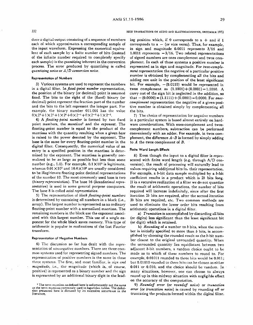
ANSI Sl .l l-l 986 29
332 IEEE TRANSACTIONS ON AUDIO AND ELECTROACOUSTICS. DECEMBER 1972
duce a digital output consisting of a sequence of numbers each of which approximates a corresponding sample of the input waveform. Expressing the numerical equiva- lent of each sample by a finite number of bits (instead of the infinite number required to completely specify each sample) is the quantizing inherent in the conversion process. The error produced by quantizing is called quantizing noise or A/D conversion noise.
Representation of Numbers
3) Various systems are used to represent the numbers in a digital filter. In fixed-p&l number representation, the position of the binary (or decimal) point is assumed fixed. The bits to the right of the (fixed) binary (or decimal) point represent the fraction part of the number and the bits to the left represent the integer part. For example, the binary number 011.001 has the value 0x2*+1 X2’+1X2~+OX2-‘+OX2-*+lX2-3.
4) A Joating-point number is formed by two fixed point numbers, the mantissa’ and the exponent. The floating-point number is equal to the product of the mantissa with the quantity resulting when a given base is raised to the power denoted by the exponent. The base is the same for every floating-point number in the digital filter. Consequently, the numerical value of an entry in a specified position in the mantissa is deter- mined by the exponent. The mantissa is generally nor- malized to be as large as possible but less than some number (e.g., 1.0). For example, 0.1 X lo* is legitimate, whereas 0.01 X lo3 and 10.0 X loo are usually considered to be illegitimate floating-point decimal representations of the number 10. The most commonly used base is two (binary representation). The base 16 (hexadecimal repre- sentation) is used in some general purpose computers. The base 8 is called octal representation.
5) The representation of block Joating-point numbers is determined by examining all numbers in a block (i.e., array). The largest number is represented as an ordinary floating-point number with a normalized mantissa. The remaining numbers in the block use the exponent associ- ated with this largest number: This use of a single ex- ponent for the whole block saves memory. This type of arithmetic is popular in realizations of the fast Fourier transform.
Representation of Negative Numbers
6) The discussion so far has dealt with the repre- sentation of nonnegative numbers. There are three com- mon systems used for representing signed numbers. The representation of positive numbers is the same in these three systems. The first, and most familiar, is sign and magnitude; i.e., the magnitude (which is, .of course, positive) is represented as a binary number and the sign is represented by an additional binary digit in the lead-
’ ‘The term m:lntissn as defined here is unfortunately not the same as the term m;~ntissa commor~ly wed in logarithm tables. The defini- tion presented here is dictated by its extensive occurrence in the literature,
ing position which, if 0 corresponds to a + and if 1 corresponds to a - (or vice versa). Thus, for example, in sign and magnitude 0.0011 represents 3/16 and 1.0011 represents -3/16. Two related representations of signed numbers are ones complement and twos com- plement. In each of these systems a positive number is represented as in sign and magnitude. For twos-comple- ment representation the negative of a particular positive number is obtained by complementing all the bits and adding one unit in the position of the least significant bit. For example, -(O.OllO) would be represented in twos complement as (1.1001)+(0.0001) = 1.1010. A carry out of the sign bit is neglected in the addition, so that -(O.OOOO) = (1.1111)+(0.0001) =O.OOOO. For ones- complement representation the negative of a given posi- tive number is obtained simply by complementing all the bits.
7) The choice of representation for negative numbers in a particular system is based almost entirely on hard- ware considerations. With ones-complement and twos- complement numbers, subtraction can be performed conveniently with an adder. For example, in twos com- plement, the difference A-B is formed by simply adding to A the twos complement of B.
Finite Word length Effects
8) Even though the input to a digital filter is repre- sented with finite word length (e.g. through A/D con- version), the result of processing will naturally lead to values requiring addi$onal bits fo. their representation. For example, a b-bit data sample multiplied by a b-bit coefficient results in a product which is 2b bits long. If in a recursive realization of a filter we do not quantize the result of arithmetic operations, the number of bits required will increase indefinitely, since after the first iteration 2b bits are required, after the second iteration 3b bits are requiied, etc. Two common methods are used to eliminate the lower order bits resulting from arithmetic operations in a digital filter.
a) Truncation is accomplished by discarding all bits (or digits) less significant than the least significant bit (or digit) which is retained.
b) Rounding of a number to b bits, when the num- ber is initially specified to more than b bits, is accom- plished by choosing the rounded result as the b-bit num- ber closest to the original unrounded quantity. When the unrounded quantity lies equidistant between two adjacent b-bit numbers, a random choice ought to be made as to which of these numbers to round to. For example, 0.01011 rounded to three bits would be 0.011; but 0.01010 rounded to three bits can be chosen as either 0.011 or-0.010, and the choice should be random. In many situations, however, one can choose to always round up in this midway situation with negligible effect on the accuracy of the computation.
9) Roundoff error (or roundof noise) or fruncation error (or truncation noise) is caused by rounding off or truncating the products formed within the digital filter.
AMERICAN NATIONAL STANDARD 30
RABlNER el at.: DIGITAL SIGNAL PROCESSING TERbllNOLOGY
The roundoff or truncation error is sometimes well modeled as a random process. On the other hand, if the data sequence to a recursive realization of a digita filter consists of constants (e.g., zero) or some other periodi- cally repeating samples, the roundoff or truncation error is periodic and causes a deadband effect br liniit cycle in the filter output. A common type of limit cycle is a zero-input limit cycle where the output of a digital filter remains periodic and nonzero, after the input has been set to zero. Dither is a sequence of numbers that is added to the input to a recursive digital filter to ameliorate the deadband effect. Even though dither increases the mean- square error in the output, it can disrupt the pattern of roundoff errors causing the deadband effect, thereby permitting the output to return to zero.
10) Overflow occurs when a digital filter computes a number that is too large to be represented in the arith- metic used in that filter. If no compensation is made for the overffow then large errors in the filter output can result either in the form of transients or of werfEov osciZ- lations. A technique used to compensate in part for over- flow is saturalion arithme& where a sum that is too large to be represented is set equal to the largest repre- sentable number in the filter.
puting, or otherwise forming, the discrete Fourier trans- form of the sequence.
2) From thedefinition, thesequence {f(O),f(l), . . . , f(N-l)] has the DFT* {F(O), F(l), . . . , F(N--1))
N--l
F(k) = c f(n)e-j(2r/N)nks
3) It is possible to recover the original sequence from its DFT by the operation
f(n) = i Nf F(k)ei(ZrlX)nk,
k-0
giving a sequence of N samples {f(O), f(l), . . . , f(N- 1) ] as the inverse discrete Fourier transform of {F(O), F(l), - . . , F(N-1) ). The operation is called inverse discrete Fourier transformation or IDFT, and is remarkably similar in form to the discrete Fourier trans- formation.
11) Dynumic range is the ratio between the largest and smallest signals which can be represented in the filter with a given fidelity criterion. Unfortunately the fidelity criterion is often vague or unspecified.
12) The roundoff or truncation noise introduced within a digital filter produces a resultant noise at the output of the digital filter. A signal-to-noise ratio can be defined in this context, for example, as the ratio of the idea1 mean-squared output signal (filter output in the absence of any rounding) to the mean-squared output noise due to rounding or truncation. Expressing this ratio in bits, as (l/2) log? of the ratio, gives an approxi- mate indication of the number of accurate bits in the filter output. Different definitions of signal-to-noise ratio may be appropriate in different contexts.
4) Some authors have defined the DFT in related but different ways, involving e i(*rlN)nk, or a multiplicative factor of l/N or l/Jr. By considering the expressions for the DFT and IDFT it is evident that the constants l/N or l/dr and the possible use of eiQ*‘N)“* in other definitions of the DFT can easily be compensated for in th,e other definitions of the IDFT.
5) Suppose for an N-point sequence we are interested in computing its DFT, and suppose N is a composite integer
A’ = I’ x r2 x * . . x r, (47)
13) Another effect of finite word length is coejkient quantization error (or parameter puantization error), which occurs when the coefficients of a digital filter, initially specified with unlimited accuracy, are quantized by rounding or truncation. Coefficient quantization error appears as error in the digital filter’s response (e.g., impulse response, transfer function, frequency response, etc.).
where the ri are a set of factors of N, not necessarily prime factors. Of the various algorithms for computing such a DFT, some require a number of operations pro- fiortional to N 2 (-, ri (since the word proportional al- lows considerable latitude, it is not necessary to be too specific about the meaning of “operation”); such algo- rithms are called fast Fourier transforms (FFT).$ An important special case is when
,, = ,* = . . . = ,# = 2
so that
k-1
For fast Fourier transforms in this case, the propor- tionality is to N log* N.
VI. Discrete Fourier Transforms and the FFT
1) For a sequence of N numbers, possibly complex, the discrete Fourier transform (DFT) is another sequence of exactly N numbers which are the values of the z trans- form of the original finite sequence for N values of z, specifically
.
6) A subclass of FFT algorithms is known which use high speed convolution techniques to compute the DFT of a sequence through a formula in which it is expressed as a convolution. Examples of such aIgorithms are the chirp z transform and the prime algorithm.
7) In order to classify different FFT algorithms and
ably m the hterature.
z = ei(2r/.V)k 9 k = 0, 1, . . . , N - 1. (44)
Discrete Fourier transformation is the ooeration of com-
* For convenience, the notation of F(R) is used todenote DFT co- efficients rather than F(ei(*~‘M~).
* The word transform instead of algorithm is embedded ineradi- . . . .
333
n-0
2 rk --, 2 lo& N.
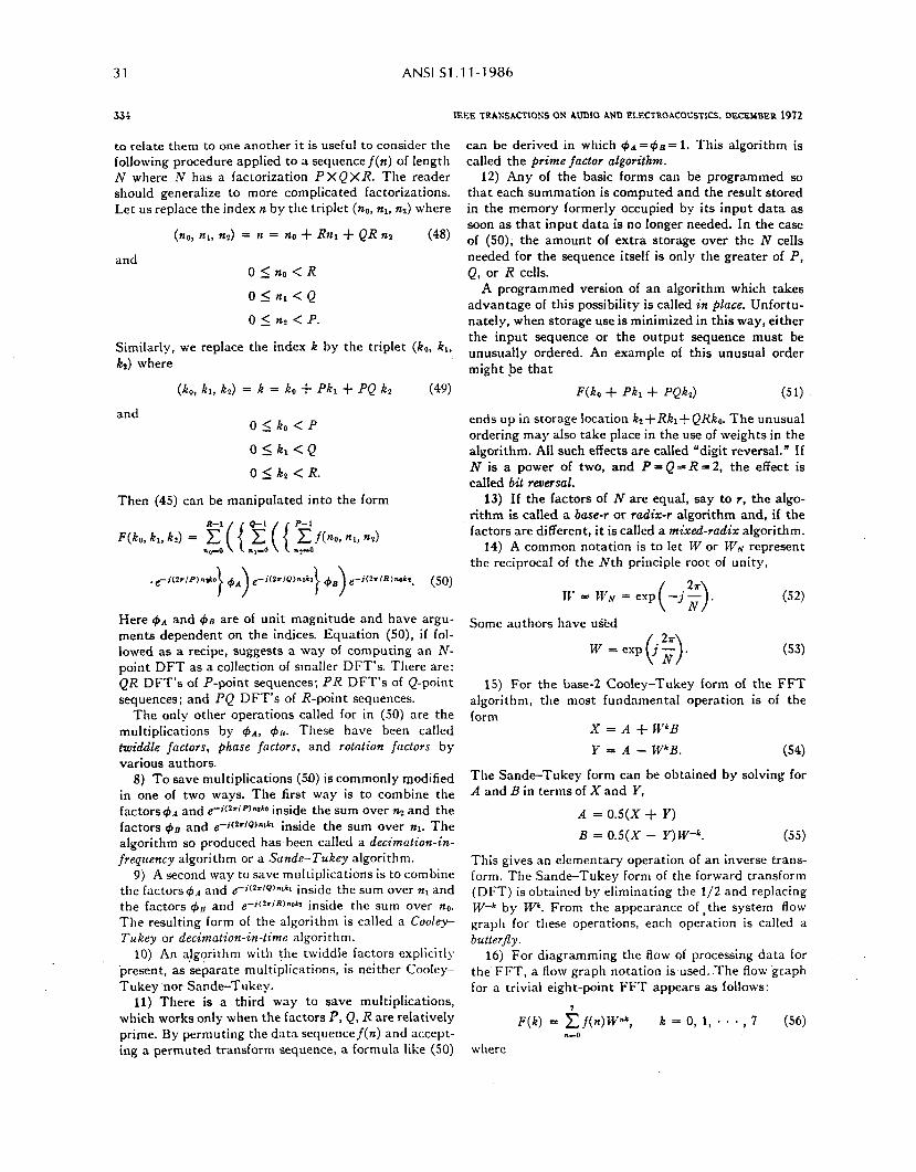
31 ANSI Sl .ll-1986
334 IEEETBANSACTIONSON AUDIO ANDELECTROACOUSTICS,DECBMBER 1972
to relate them to one another it is useful to consider the following procedure applied to a sequencej(n) of length N where N has a factorization PXQXR. The reader should generalize to more complicated factorizations. Let us replace the index n by the triplet (no, nl, nz) where
(no, nl, n2) = n = no + Rnl + QR nz (48)
and OIno<R
Ole<Q 0 I tl? < P.
Similarly, we replace the index k by the triplet (Ro. kl, kt) where
(ko, RI, k,) = k = ko + Ph + PQ kz (49)
and O<ko<P
Olh<Q 0 2 kz < R.
Then (45) can be manipulated into the form
Here +A and 40 are of unit magnitude and have argu- ments dependent on the indices. Equation (SO), if fol- lowed as a recipe, suggests a way of computing an N- point DFT as a collection of smaller DFT’s. There are: QR DFT’s of P-point sequences; PR DFT’s of Q-point sequences; and PQ DFT’s of R-point sequences.
The only other operations called for in (50) are the multiplications by +A, 4~. These have been called twiddle factors, phase factors, and rotation facfors by various authors.
8) To save multiplications (50) is commonly modified in one of two ways. The first way is to combine the factors +‘A and e- i(zr’P)n~~~ inside the sum over n2 and the factors 40 and e-j(2rlQ)nlrl inside the sum over nl. The algorithm so produced has been called a decimalion-in- jreqzrency algorithm or a Sunde-Tukey algorithm.
9) A second way to save multiplications is to combine the factors 4A and e--i(tr/Q)n+t inside the sum over n, and the factors 4~ and e--i(2rlR)no*1 inside the sum over nO. The resulting form of the algorithm is called a Cooley- Tukey or decimation-in-time algorithm.
10) An aJg?rithm with the twiddle facfors explicitl) ‘present, as separate multiplications, is neither Cooley- Tukey nor Sande-Tukey.
11) There is a third way to save multiplications, which works only when the factors P, Q, R are relatively prime. By permuting the data sequencej(n) and accept- ing a permuted transform sequence, a formula like (SO)
can be derived in which +A =$~a = 1. This algorithm is called the prime factor algorithm.
12) Any of the basic forms can be programmed so that each summation is computed and the result stored in the memory formerly occupied by its input data as soon as that input data is no longer needed. In the case of (50); the amount of extra storage over the N cells needed for the sequence itself is only the greater of P, Q, or R cells.
A programmed version of an algorithm which takes advantage of this possibility is called in place. Unfortu- nately, when storage use is minimized in this way, either the input sequence or the output sequence must be unusually ordered. An example of this unusual order might be that
Wo + Pk, + J’QkJ (5 1)
ends up in storage location kt+RkI+QRka. The unusual ordering may also take place in the use of weights in the algorithm. All such effects are called “digit reversal.” If N is a power of two, and P = Q = R = 2, the effect is called bit reversal.
13) If the factors of N are equal, say to I, the algo- rithm is called a base-r or radir-r algorithm and, if the factors are different, it is called a mixed-radix algorithm.
14) A common notation is to let W or WN represent the reciprocal of the Nth principle root of unity,
Some authors have u&d
(53)
15) For the base-2 Cooley-Tukey form of the FFT algorithm, the most fundamental operation is of the form
X = A + WkB
Y A = - W’B. (54)
The Sande-Tukey form can be obtained by solving for A and B in terms of X and Y,
A = 0.5(X + Y)
B = 0.5(X - Y)W-“. W
This gives an elementary operation of an inverse trans- form. The Sande-Tukey form of the forward transform (DFT) is obtained by eliminating the l/2 and replacing W-k by Wk. From the appearance of *the system flow graph for these operations, each operation is called a butterfly.
16). For diagramming the flow of processing data for the FFT, a flow graph notation is used. The flow graph for a trivial eight-point FFT appears as follows:
F(k) = &z)Wnk, k=0,1,+..,7 (56)
where
n-II
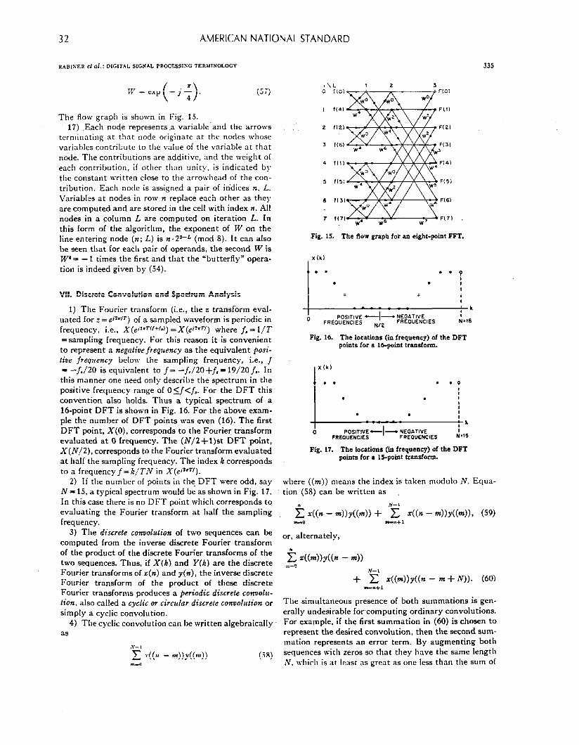
32 AMERICAN NATIONAL STANDARD
RABISER et al.: DIGITAL SIGNAL PROCESSISG TERMIXOLOCY 335
w = exp - j $ . ( >
(57)
The flow graph is shown in Fig. 15. 17) E.ach node represents.a variable and the arrows
terminating at that node originate at the nodes whose variables contribute to the value of the variable at that node. The contributions are additive, and the weight of each contribution, if other than unity, is indicated b) the constant written close to the arrowhead of the con- tribution. Each node is assigned a pair of indices tl, L. Variables at nodes in row n replace each other as they are computed and are stored in the cell with index S. All nodes in a column L are computed on iteration L. In this form of the algorithm, the exponent of W on the line entering node (n; L) is n.2s-L (mod 8). It can also be seen that for each pair of operands, the second W is W’= -1 times the first and that the “butterfly” opera- tion is indeed given by (34).
VII. Discrete Convolution and Spectrum Analysis
1) The Fourier transform (i.e., the .a transform eval- uated for s = ei?r’r) of a sampled waveform is periodic in frequency, i.e., X(ei2rT(l+fd) =X(ei2rV) where f, I l/T =sampling frequency. For this reason it is convenient to represent a negntive ffeqtrency as the equivaIent posi- tive freqzcency below the sampling frequency, i.e., f = -J./Z0 is equivalent to f= --f,/2O+f,= 19/2Of,. In this manner one need only describe the spectrum in the positive frequency range of Osf<f,. For the DFT this convention also holds. Thus a typical spectrum of a 1Qpoint DFT is shown in Fig. 16. For the above exam- ple the number of DFT points was even (16). The first DFT point, X(O), corresponds to the Fourier transform evaluated at 0 frequency. The (N/2+l)st DFT point, X(N/2), corresponds to the Fourier transform evaIuated at half the sampling frequency. The index k corresponds to a frequency f = k/TN in X(ejzrT’).
2) If the number of points in the DFT were odd, say N = 15, a typical spectrum would be as shown in Fig. 17. In this case there is no DFT point which corresponds to evaluating the Fourier transform at half the sampling frequency.
3) The discrete convolution of two sequences can be computed from the inverse discrete Fourier transform of the product of the discrete Fourier transforms of the two sequences. Thus, if X(k) and Y(k) are the discrete Fourier transforms of x(n) and y(n), the inverse discrete Fourier transform of the product of these discrete Fourier transforms produces a periodic discrete conuolu- lion, also called a cyclic or circzclar discrete convolution or simply a cyclic convolution.
4) The cyclic convolution can be written algebraically BS
N- 1 c .d(N - d)Y((d) (3
l\L I 2 3 0 1101 F(O)
WO
I f(4) F(t)
2 1121 F(2)
3 f(6) F(31 3
Fig. 15. The flow graph for an eight-point FFT.
x(k)
. . l l P
. . I
I . . 1
’ k
0 POSITIVE -I- $$$$ES : FREOIJENCIES N12
N’l6
Fig. 16. The locations (ii frequency) of the DFT points for a M-point trsnsfom.
I x(k)
. . . l ?
. I . . I I . -- z i k
6 POSITIVE .-I- NEGATIVE FREOUENCIES FREOUENCIES fLs
Fig. 17. The locations (ii frequency) of the DFT points for a IS-point transfom.
where ((m)) means the index is taken modulo N. Equa- tion (58) can be written as
n N-I
C r((n - 4)YW) + c d(n - d)Y((d), (59) m-0
or, alternately,
m”n+ I
+ x z(W)r((n - m + NJ). (60) -n+ 1
The simultaneous presence of both summations is gen- erally undesirable for computing ordinary convolutions. For example, if the first summation in (60) is chosen to represent the desired convolution, then the second sum- mation represents an error term. By augmenting both sequences with zeros so that they have the same length N, which is at least as great as one less than the sum of
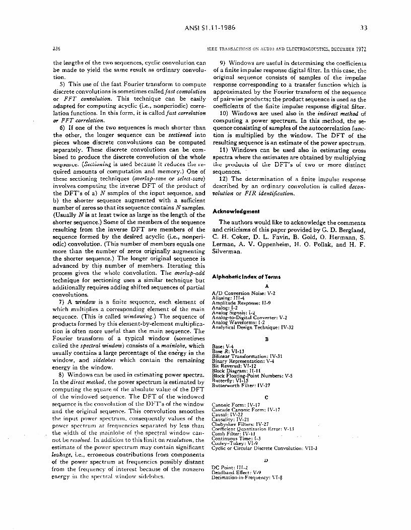
ANSI Sl .l l-1 986 33
336 IEEE TRANSACTIONS OS AtiDIO AKD ELECTROACOWTICS, DECEMBER 1972
the lengths of the two sequences, cyclic convolution can be made to yield the same result as ordinary convolu- tion.
5) This use of the fast Fourier transform to compute discrete convolutions is sometimes calledfast convol&ion or FFT convolzrtion. This technique can be easily adapted for computing acyclic (i.e., nonperiodic) corre- lation functions. In this form, it is called fast correhztion or FFT correlation.
6) If one of the two sequences is much shorter than the other, the longer sequence can be sectioned into pi&es whose discrete convolutions can be computed separately. These discrete convolutions can be com- bined to produce the discrete convolution of the whole sequence. (Sectioning is used because it reduces the re- quired amounts of computation and memory.) One of these sectioning techniques (owerlap-save or select-save) involves computing the inverse DFT of the product of the DFT’s of a) N samples of the input sequence, and b) the shorter sequence augmented with a sufficient number of zeros so that its sequence contains N samples. (Usually N is at least twice as large as the length of the shorter sequence.) Some of the members of the sequence resulting from the inverse DFT are members of the sequence formed by the desired acyclic (i.e., nonperi- odic) convolution. (This number of members equals one more than the number of zeros originally augmenting the shorter sequence.) The longer original sequence is advanced by this number of members. Iterating this process gives the whole convolution. The overlap-add technique for sectioning uses a similar technique but additionally requires adding shifted sequences of partial convolutions.
7) A window is a finite sequence, each element of which multiplies a corresponding element of the main sequence. (This is called windowing.) The sequence of products formed by this element-by-element multiplica- tion is often more useful than the main sequence. The Fourier transform of a typical window (sometimes called the spectral tindow) consists of a mainlobe, which usually contains a large percentage of the ene’rgy in the window, and sidelobes which contain the remaining energy in the window.
8) Windows can be used in estimating power spectra. In the direct mefhod, the power spectrum is estimated by computing the square of the absolute value of the DFT of the windowed sequence. The DFT of the windowed sequence is the convolution of the DFT’s of the window and the original sequence. This convolution smoothes the input power spectrum, consequently values of the power spectrum at frequencies separated by less than the width of the mainlol)e of the spectral window can- not be resolved. In addition to this limit on resolulion, the estimate of the power spectrum may contain significant leaktrge, i.e., erroneous contributions from components of the power spectrum at frequencies possibly distant from the frequency of interest because of the nonzero energy in tllc spectral \vindo\v sidclolxs.
9) Windows are useful in determining the coefficients of a finite impulse response digital filter. In this case, the original sequence consists of samples of the impulse response corresponding to a transfer function which is approximated by the Fourier transform of the sequence of pairwise products; the product sequence is used as the coefficients of the finite impulse response digital filter.
10) Windows are used also in the indirect method of computing a power spectrum. In this method, the se- quence consisting of samples of the autocorrelation func- tion is multiplied by the window. The DFT of the resulting sequence is an estimate of the power spectrum.
11) Windows can be used also in estimating cross spectra where the estimates are obtained by multiplying the products of the DFT’s of two or more distinct sequences.
12) The determination of a finite impulse: response described by an ordinary convolution is called decon- volution or FIR identification.
Acknowledgment
The authors would like to acknowledge the comments and criticisms of this paper provided by G. D. Bergland, C. H. Coker, D. L. Favin, B. Gold, 0. Hermann, S. Lerman, A. V. Oppenheim, H. 0. Pollak, and H. F. Silverman.
Alphabetic Index of Terms
A A/D Conversion Noise: V-2 Aliasing: III-4 Amplitude Response: II-9 Analog: I-2 Analog Signals: 1-2 Analog-to-Digital Converter: V-2 Analog Waveforms: I-2 Analytical Design Technique: IV-32
B Base: V-4 Base R: VI-13 Bilinear Transformation: IV-31 Binary Representation: V-4 Bit Reversal: VI-12 Block Diagram: II-11 Block Floating-Point Numbers: V-S Butterfly: VI-15 Butterworth Filter: IV-27
C Canonic Form : IV- 17 Cascade Canonic Form: IV-17 Causal: IV-22 Causality: IV-21 Chebyshev Filters: IV-27 Coefficient Quantization Error: V-13 Comb Filter: IV-11 Continuous Time: I-3 Cooley-Tukey: VI-9 Cyclic or Circular Discrete Convolution: VII-3
D DC Point: III-2 Deadband Effect: V-9 Decim.ltion-in-Frgllellc~: VI-8
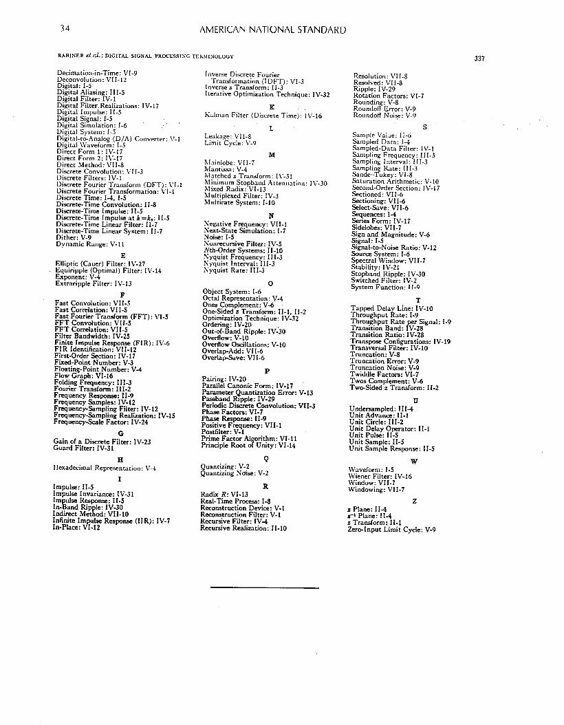
AMERICAN NATIONAL STANDARD
UBINER el Cl.: DIGITAL SIGNAL PROCESSISG TEK.\IINOLOtiY 337
Decimation-in-Time: VI-9 Deconvolution: VII-12 Digital: I-5 Digital Aliasing: III-5 Digital Filter: IV-l Digital Filter.Realizations: IV-17 Digital Impulse: II-3 Digital Signal: I-S Digital Simulation: I-6 Digital System: I-5 Digital-to-Analog (D/A) Converter: V-1 Digital \Vaveform: I-5 Direct Form 1: IV-17 Direct Form 2: IV-17 Direct Method: VII-8 Discrete Convolution: VI I-3 Discrete Filters: IV-1 Discrete Fourier Transform (DFT): \‘I-1 Discrete Fourier Transformation: VI-1 Discrete Time: I-4, I-5 Discrete-Time Convolution: II-8 Discrete-Time Impulse: II-5 Discrete-Time Impulse at k =k.: I I-3 Discrete-Time Linear Filter: II-7 Discrete-Time Linenr System: II-7 Dither: V-9 Dynamic Range: V-l I
E Elliptic (Cauer) Filter: I\‘-27 Equiripple (Optimal) Filter: IV-14 Exponent: V-4 Extraripple Filter: IV-13
P Fast Convolution: VII-S Fast Correlation: VII-S Fast Fourier Transform (FFT) : VI-S FFT Convolution: VII-5 FFT Correlation: VII-S Filter Bandwidth: IV-25 Finite Impulse Response (FIR): IV-6 FIR Identification: VII-12 First-Order Section: IV-17 Fixed-Point Number: V-3 Floating-Point Number: V-4 Flow Graph: VI-16 Folding Frequency: III-3 Fourier Transform : I I I-2 Frequency Response: II-9 Frequency Samples: IV-12 Frequency-Sampling Filter: IV-12 Frequency-Sampling Realization: IV-15 Frequency-Scale Factor: IV-24
G Gain of a Discrete Filter: IV-23 Guard Filter: IV-31
H Hexadecimal Representation: V-4
I Impulse: II-5 Impulse Invariance: IV-31 Impulse Response: II-5 In-Band Ripple: IV-30 Indirect Method: VII-10 Infinite Impulse Response (IIR): IV-7 In-Place: VI-12
Inverse Discrete Fourier Transformation (IDFT): VI-3
inverses Transform: II-3 Iterative Optimization Technique: IV-32
K Kalman Filter (Discrete Time): IV-16
L Leakage: VII-8 Limit Cycle: \‘-9
M hiainlobe: VII-7 Mantissa: V-4 Matched s Transform: I\‘-31 Minimum Stopband Attenuation: IV-30 Mixed Radix: VI-13 Multiplexed Filter: IV-3 Multirate System: I-10
N Negative Frequency: VII-1 Next-State Simulation: I-7 Noise: I-S Sonrecursive Filter: IV-S Nth-Order Systems: II-10 Nyquist Frequency: III-3 Nyquist Interval: III-3 Nyquist Rate: III-3
0 Object System: I-6 Octal Representation: V-4 Ones Complement: V-6 One-Sided .s Transform: 11-1, II-2 Optimization Technique: IV-32 Ordering: IV-20 Out-of-Band Ripple: IV-30 Overflow: V-10 Overflow Oscillations: V-10 Overlap-Add: VII-6 Overlap-Save: VI I-6
P Pairing: IV-20 Parallel Canonic Form: IV-i7 Parameter Quantisation Error: Passband Ripple: IV-29 Periodic Discrete Convolution: Phase Factors: VI-7 Phase Response: II-9 Positive Frequency: VII-1 Postfilter: V-l Prime Factor AI orithm: VI-11 Principle Root o f Unity: VI-14
Q Quantizing: V-2 Quantizing Noise: V-2
R Radix R: VI-13 Real-Time Process: I-8 Reconstruction Device: V-l Reconstruction Filter: V-l Recursive Filter: IV-l Recursive Realization: II-10
v-13
VII-3
Resolution: VII-8 Resolved: VII-8 Ripple: IV-29 Rotation Factors: VI-7 Rounding: V-8 Roundoff Error: V-9 Roundoff Noise: V-9
s Sample Value: 11-6 Sampled Data: I-4 Sampled-Data Filter: IV-1 Sampling Frequency: III-3 Sampling Interval: III-3 Sampling Rate: I II-3 Sande-Tukey: VI-8 Saturation Arithmetic: V-10 Second-Order Section: IV-l 7 Sectioned: VII-6 Sectioning: VII-6 Select-Save: VII-6 Sequences: I-4 Series Form: IV-17 Sidelobes: VII-7 Sign and Magnitude: V-6 Signal: I-5 Signal-to-Noise Ratio: V-12 Source System: I-6 Spectral Window: VII-7 Stability: IV-21 Stopband RippIe: IV-30 Switched Filter: IV-2 System Function: 11-o
T Tapped Delay Line: IV-10 Throughput Rate: I-9 Throughput Rate per Signal: I-9 Transition Band: IV-28 Transition Ratio: IV-28 Transpose Configurations: IV-19 Transversal Filter: IV-10 Truncation: V-8 Truncation Error: V-9 Truncation Noise: V-9 Twiddle Factors: VI-7 Twos Complement: V-6 Two-Sided s Transform : I I-2
TJ Undersampled: III-4 Unit Advance: II-1 Unit Circle: III-2 Unit Delay Operator: II-1 Unit Pulse: II-S Unit Sample: II-S Unit Sample Response: II-5
W Waveform: I-S Wiener Filter: IV-16 Window: VII-7 Windowing: VII-7
z
s Plane: II-4 s+ Plane: II-4 s Transform: II-1 Zer*Input Limit Cycle: V-9

NOTES 35

36 NOTES

NOTES 37
38
ACOUSTICAL SOCIETY OF AMERICA STANDARDS SECRETARIAT
The Standards Program of the Acoustical Society of America is the responsibility of the ASA’s Committee on Standards (ASACOS) and is executed by ASA’s Standards Secretariat headed by its Standards Manager.
The Acoustical Society of America holds the Secretariat for four accredited standards committees of the Ameri- can National Standards Institute (ANSI); Sl on Acoustics, S2 on Mechanical Shock and Vibration, S3 on Bio- acoustics, and S12 on Noise; and provides the United States input to ISO/TC 43 on Acoustics, for which Sl and 53 serve as Technical Advisory Groups, and S12 serves as the Technical Advisory Group for ISO/TC43/ SC1 Noise. ASA also administers the international secretariat of ISO/TC 108 on Mechanical Vibration and Shock (on behalf of the American National Standards Institute) and provides the U.S. input via the Technical Advisory Group for ISO/TC 108, which is Standards Committee S2 (Standards Committee S3 is the Technical Advisory Group for ISO/TC108/SC4 Human Exposure to Mechanical Vibration and Shock).
Standards are produced in four broad areas: physical acoustics, mechanical shock and vibration, bioacoustics, and noise, and are reaffirmed or revised every five years. The latest information on current ANSI standards as well as those under preparation is available from the Standards Secretariat.
When ordering ANSI Sl.ll-1986, please also use ASA Catalog No. 65-1986 for easy reference. This standard and other standards listed in the ASA Standards Catalog may be ordered from the following address:
Publication Sales, Dept. STD American Institute of Physics
335 East 45th Street New York, New York 10017
Telephone: (516) 349-7800
Standards listed in the ASA Standards Catalog can be ordered by out-of-state customers by calling the Ameri- can Institute of Physics WATS number, l-800-AIP-PHYS Toll Free. Also, AIP accepts major credit cards (American Express, VISA, Mastercard) with a minimum order of $10.00.
If you wish to have further information on the Standards Publication Program of the Acoustical Society of America, address your inquiries to
Standards Manager Standards Secretariat
Acoustical Society of America 335 East 45th Street
New York, New York 10017 Telephone: (212) 661-9404