RATIONAL AND INTEGRAL POINTS ON CURVES

Andrew Granville

Abstract. These are notes from a course given in Autumn of 2011 at the Universite deMontreal. I have written things fairly completely up to about chapter 15. There is a lotmore to be added on elliptic curves, and then on higher degree curves. Also stuff on integral

points via Diophantine approximation. Please email me with any corrections or remarks(andrew@dms.umontreal.ca).

Table of ContentsPreface. Diophantine equations and curves

Chapter 1. Linear equations

1.1. Linear equations in two unknowns1.2. The Euclidean algorithm1.3. Several simultaneous linear equations in several unknowns1.4. Rational solutions and lattices

Chapter 2. Some useful mathematics

2.1. Rational approximations to real numbers2.2. The Irrationality of

√d.

2.3. Continued fractions for real numbers2.4. Solving the cubic. Pre-cursors to Galois theory.2.5. Constructibility and Galois theory2.6. Resultants and Discriminants2.7. Mobius transformations: Lines and circles go to lines and circles2.8. Groups2.9. Ideals

Chapter 3. Quadratic equations3.1. The Pythagorean equation3.2. Fermat’s “infinite descent”3.3. Squares mod m3.4. The law of quadratic reciprocity3.5. Sums of two squares3.6. The values of x2 + dy2

Typeset by AMS-TEX

2

3.7. Solutions to quadratic equations3.8. Pell’s equation3.9. Descent on solutions of x2 − dy2 = n, d > 0

Chapter 4. Binary quadratic forms

4.1. Representation of integers by binary quadratic forms4.2. Equivalence classes of binary quadratic forms4.3. Class number one4.4. Ideals in quadratic fields4.5. Composition laws4.6. Bhargava composition4.7. The idoneal numbers4.8. SL(2,Z)-transformations. Forms-Ideals-Transformations4.9. The ring of integers of a quadratic field, revisited

Chapter 5. Real quadratic fields

5.1. Quadratic irrationals and periodic continued fractions5.2. Pell’s equation5.3. The size of solutions to Pell’s equation5.4. More examples of Pell’s equation5.5. Binary quadratic forms with positive discriminant, and continued fractions

Chapter 6. L-functions and class numbers

6.1. Counting solutions to Pell’s equation (a heuristic)6.2. Dirichlet’s class number formula6.3. The class number one problem in real quadratic fields6.4. Dirichlet L-functions

Chapter 7. More about quadratic forms and lattices

7.1. Minkowski and lattices7.2. The number of representations as the sum of two squares7.3. The number of representations by arbitrary binary quadratic forms7.4. The number of representations as the sum of three squares7.5. The number of representations as the sum of four squares7.6. Universality of quadratic forms7.7. Representation by positive definite quadratic forms7.8. Descent and the quadratics.

Chapter 8. More useful mathematics

8.1. Finite fields8.2. Affine vs. Projective8.3. Lifting solutions

Chapter 9. Counting points mod p

3

9.1. Linear and quadratic equations mod p9.2. The diagonal cubic equation mod p9.3. The equation y2 = x3 + ax9.4. The equation y2 = x3 + b9.5. Counting solutions mod p9.6. Degenerate elliptic curves mod p9.7. Lifting solutions9.8. Simultaneous Pell equations

Chapter 10. Power series, partitions, and magical modularity

10.1. Partitions10.2. The numerology of partitions10.3. Generating functions for binary quadratic forms, and L-functions10.4. Poisson’s summation formula and the theta function10.5. Jacobi’s powerful triple product identity10.6. An example of modularity: y2 = x3 − x

Chapter 11. Degree three curves — why the curve y2 = x3 + ax+ b?

11.1. Parametric families of rational points on curves11.2. Constructing new rational points on cubic curves from old ones11.3. Cubic curves into Weierstrass form11.4. Diagonal cubic curves11.5. y2 equals a quartic with a rational point11.6. The intersection of two quadratic polynomials in three variables (that is, the

intersection of two quadratic surfaces)11.7. Doubling a point on a diagonal cubic

Chapter 12. The group of rational points on an elliptic curve

12.1. The group of rational points on an elliptic curve12.2. The group law on the circle, as an elliptic curve12.3. No non-trivial rational points by descent12.4. The group of rational points of y2 = x3 − x12.5. The arithmetic of a torsion point12.6. Embedding torsion in Fp12.7. The size of rational points

Chapter 13. Mordell’s theorem – E(Q) is finitely generated

13.1. The proof of Mordell’s Theorem over the rationals13.2. Another example: Four squares in an arithmetic progression13.3. Mordell’s Theorem in number fields13.4. More precise bounds on naive height13.5. Neron-Tate height13.6. An inner product13.7. The number of points in the Mordell-Weil lattice up to height x

4

13.8. Magic squares and elliptic curves

Chapter 14. The Weierstrass ℘-function, and endomorphisms of ellipticcurves

14.1. Double periodicity and the Weierstrass ℘-function.14.2. Parametrizing elliptic curves14.3. Torsion points in C14.4. The converse theorem14.5. Maps between elliptic curves over C. Complex multiplication.14.6. Homomorphisms and endomorphisms for elliptic curves14.7. The Frobenius map and the number of points on E(Fpk)14.8. Classifying endomorphisms when t = 014.8b Attempt at supersingular primes (needs work)14.9. Torsion points in Fp

Chapter 15. Modular Forms

15.1. The magic of Eisenstein series15.2. The Fourier expansion of an Eisenstein series15.3. Modular forms15.4. Determining spaces of modular forms15.5. The j-function15.6. The j-invariant and complex multiplication15.7. Almost an Eisenstein series15.8. Sublattice and subgroups15.9. Hecke operators15.10. The Mellin transform and the construction of L-functions15.11. Congruence subgroups

Chapters 16, 17, 18. More stuff on elliptic curves

Chapter 19. Integral points on elliptic curves

19.1. Sums of two cubes19.2. Taxicab numbers and other diagonal surfaces

Chapter 20. Integral points on higher genus curves

20.1. Thue’s Theorem

Chapter 21. Diophantine equations in polynomials

Chapter 22. Fermat’s Last Theorem

21.1. FLT and Sophie Germain21.2. The abc-conjecture21.3. Faltings’ Theorem nee Mordell’s conjecture

5

Preface

It is natural for a mathematician to ask for the solutions to a given equation. To un-derstand the solutions in complex numbers may require ideas from analysis; to understandthe solutions in integers requires ideas from number theory. The main difference is that,in the complex numbers, one can solve equations by using limits. For example to find acomplex number x for which x2 = 2 we need to find increasingly good approximations toa solution, in order to prove that

√2, the limit of the approximations, exists. However

to prove that there is no rational number p/q such that (p/q)2 = 2 takes rather differenttechniques, and these are what we focus on in these notes.

Finding integral or rational solutions to a polynomial equation (or finite set of poly-nomial equations) is known as Diophantine arithmetic in honour of Diophantus,1 a Greekmathematician who lived in Alexandria in the third century A.D.2 His thirteen volumeArithmetica dealt with solutions to equations in integers and rationals,3 which are nowknown as Diophantine equations.

Typically the subject of Diophantine equations is motivated by the quest to prove thatthere are no integer solutions to certain Diophantine equations. For example, Catalan’s1844 conjecture that the only integer solution to

xp − yq = 1

with x, y ≥ 1 and p, q ≥ 1 is 32 − 23 = 1; which was proved by Preda Mihailescu in 2002.Also Fermat’s assertion from around 1637, known as “Fermat’s Last Theorem”,4 that thereare no integers x, y, z ≥ 1 and n ≥ 3 for which

xp + yp = zp,

which was finally proved in 1995 by Sir Andrew Wiles.Our goals will not be so elevated. We will mostly focus on the beautiful theory for

trying to find rational solutions to Diophantine equations in just two variables, of degreesone, two and three. Degree one equations are more-or-less completely understood, butthere are fundamental questions for degrees two and three that remain open, and indeedunderstanding degree three equations is perhaps the most researched problem in modernnumber theory.

We shall assume that the reader is familiar with a first course in number theory. Whenwe require more advanced concepts we shall explain them.

1Bachet’s 1621 Latin translation of Diophantus’sArithmetica helped spark the mathematical Renaissance.2Many of the most famous ancient “Greek mathematicians”, such as Diophantus, Eratosthenes,

Euclid, Hero, Pappus, and Ptolemy, actually worked in Alexandria, Egypt.3Though only parts of six of the volumes have survived.4Indeed he wrote “it is impossible to separate a cube into two cubes, or a fourth power into two

fourth powers, or in general, any power higher than the second, into two like powers. I have discovered a

truly marvelous proof of this, which this margin is too narrow to contain” in his copy of Arithmetica. Acopy of Arithmetica with Fermat’s notes was published after his death, by his son in 1670.

1

1. Linear equations

1.1. Linear equations in two unknowns. The simplest Diophantine problem oneencounters is to ask whether, given non-zero integers a, b and integer c, there are solutionsin integers m,n to

(1.1) am+ bn = c .

One encounters this problem in a first course in number theory, and proves that there aresuch solutions if and only if gcd(a, b) divides c. We shall investigate this question againnow, with a slightly different tilt to our discussion.

The first step in any Diophantine problem is to note that we may divide the coefficientsby their greatest common divisor, and not change the solutions to the equation; in thiscase the coefficients are a, b, c and so, after dividing through by their gcd, we may assumethat gcd(a, b, c) = 1. In this case, our goal is to prove that (1.1) has integer solutions m,nif and only if gcd(a, b) = 1:

Suppose that there exists integers m,n for which am+ bn = c. Now gcd(a, b) dividesboth a and b, and so divides any linear combination of them, in particular am + bn = c.But then gcd(a, b) divides gcd(gcd(a, b), c) = gcd(a, b, c) = 1.

Now suppose that gcd(a, b) = 1. Since gcd(a, b) = 1, therefore there exists an inverseto b (mod a); that is an integer v for which bv ≡ 1 (mod a) and hence there exists aninteger u for which au+ bv = 1. Then we have a solution to (1.1) with m = cu, n = cv

This proof establishes that there are solutions to the Diophantine equation am+bn = 1when gcd(a, b) = 1 without necessarily finding any solutions. Of course we can explicitlydetermine a solution using the Euclidean algorithm (which we discuss below).

Once one has found one solution to this Diophantine equation, then naturally onewishes to find all solutions. This is not difficult by “comparing solutions”. To do this westart with a base solution (r, s) and write every other solution as (r + x, s+ y), so that

ax+ by = (a(r + x) + b(s+ y))− (ar + bs) = c− c = 0.

This is another Diophantine problem so dividing through a and b by gcd(a, b) we obtainAx = −By where A = a/g, B = b/g with g := gcd(a, b). Now B divides Ax and (B,A) = 1so that B divides x. Writing x = tB for some integer t, we have y = −tA and hence allsolutions to am+ bn = c are given by

m = r + tb

(a, b), n = s− t

a

(a, b)where t is an integer.

There is another way to write the result for solvability of (1.1):

The Local-Global Principal for Linear Equations. Let a, b, c be given integers, witha, b = 0 and gcd(a, b, c) = 1. There are solutions in integers m,n to am+bn = c if and onlyif for all prime powers pe there exist residue classes u, v (mod pe) such that au + bv ≡ c(mod pe) and gcd(u, v, p) = 1.

2

This is called a Local-Global Principal because the solubility of the Diophantine equa-tion over the integers, an infinite (global) ring, is equivalent to the solubility of the Dio-phantine equation over the integers mod pe, each a finite (local) ring.

Proof. Suppose that am+ bn = c, so that am+ bn ≡ c (mod pe) for all prime powers pe.Either this solution satisfies (m,n, p) = 1, or we can take a(m− b)+ b(n+a) ≡ c (mod pe)in which case (m− b, n+ a, p) = 1, else p divides (a, b, c) = 1 which is impossible.

On the other hand suppose that for each prime power pe dividing b we have a solutionup, vp to aup + bvp ≡ c (mod pe). By the Chinese Remainder Theorem there exist residueclasses u, v (mod b) such that u ≡ up, v ≡ vp (mod pe) for each pe∥b, and so au+ bv ≡ c(mod b). Now given any integer m ≡ u (mod b) we note that am ≡ au ≡ c (mod b) andso there exists an integer n for which am+ bn = c.

At first sight a big drawback of this re-formulation is that we are going to determinesolubility over the integers, an infinite number of possibilities, by studying an infinitenumber of finite questions (i.e. modular arithmetic). However the proof makes it clear thatwe actually only need to study a finite number of cases, those prime powers dividing b.Hence we might have simply stated that there are solutions in integers m,n to am+bn = cif and only if there exist residue classes u, v (mod b) such that au+ bv ≡ c (mod b) withgcd(u, v, b) = 1.

We will take a similar approach to quadratic equations.

1.2. The Euclidean Algorithm. To determine the greatest common divisor of twointegers a ≥ b ≥ 1, we write a = qb+ r where q and r are integers with 0 ≤ r ≤ q − 1.

Exercise 1.2.1. Prove that gcd(a, b) = gcd(b, r).

Now since r < b ≤ a, our new pair of integers (b, r) is smaller than the original pair (a, b)and so we can iterate this observation, until the smaller of the two numbers divides thelarger. In that case we know that gcd(b, a) = b. In this way we can determine the gcd ofany two given positive integers. For example:

85 = 1 · 48 + 37, so that gcd(85, 48) = gcd(48, 37);

48 = 1 · 37 + 11, so that gcd(48, 37) = gcd(37, 11);

37 = 3 · 11 + 4, so that gcd(37, 11) = gcd(11, 4);

11 = 2 · 4 + 3, so that gcd(11, 4) = gcd(4, 3);

4 = 1 · 3 + 1, so that gcd(4, 3) = gcd(3, 1) = 1.

We now wish to show how to find integers m,n such that am+ bn = gcd(a, b), by iteratingbackwards in the above algorithm. We start with the observation that if a = bq then0 · a + 1 · b = b = gcd(a, b). We also note that if a = qb + r and bu − rv = 1 for someintegers u and v. Then

gcd(a, b) = gcd(b, r) = bu− rv = bu− (a− qb)v = b(u+ qv)− av,

the desired linear combination of a and b. For the above example we start with 1 = 0·3+1·1

3

and together

with 4 = 1 · 3 + 1 =⇒ 1 = 0 · 3 + 1 · (4− 1 · 3) = 1 · 4− 1 · 3;with 11 = 2 · 4 + 3 =⇒ 1 = 1 · 4− 1 · (11− 2 · 4) = 3 · 4− 1 · 11;with 37 = 3 · 11 + 4 =⇒ 1 = 3 · (37− 3 · 11)− 1 · 11 = 3 · 37− 10 · 11;with 48 = 1 · 37 + 11 =⇒ 1 = 3 · 37− 10 · (48− 1 · 37) = 13 · 37− 10 · 48;with 85 = 1 · 48 + 37 =⇒ 1 = 13 · (85− 1 · 48)− 10 · 48 = 13 · 85− 23 · 48.

One useful consequence of the Euclidean algorithm is an understanding of the set of linearcombinations of two integers

I(a, b) := am+ bn : m,n ∈ Z.

This is called the ideal generated by a and b over Z. We observe that if a = bq + rthen I(a, b) = I(b, r): for then am + bn = (bq + r)m + bn = b(n + qm) + rm so thatI(a, b) ⊂ I(b, r), and bu + rv = bu + (a − bq)v = av + b(u − qv) so that I(b, r) ⊂ I(a, b).Following through the steps of the Euclidean algorithm we then have that

I(a, b) = I(g), where g := gcd(a, b).

One can view the step as showing that there is a 1-to-1 correspondence between the integersolutions to am+ bn = c and the integer solutions to bu+ rv = c, via the invertible lineartransformation (

uv

)=

(q 11 0

)(mn

)⇐⇒

(mn

)=

(0 11 −q

)(uv

).

The notion of ideal generalizes to I(a1, . . . ak) := a1m1+ . . .+ akmk : m1, . . . ,mk ∈Z for any finite set of generators a1, . . . , ak, and this equals I(g) where g =gcd(a1, . . . ak);this implies there exist integers m1, . . . ,mk such that a1m1 + . . .+ akmk = g.

There are compact (and useful) ways to represent the Euclidean algorithm. We beginagain with integers a > b > 1 but now for which (a, b) = 1. Again if a = bq + r withb > r ≥ 1 then

a

b= q+

r

b= q+

1br

.

We can repeat this to replace b/r by such a fraction, and iterate, until our fraction is aninteger. We therefore obtain the continued fraction

a

b= a0+

1

a1+1

a2+1

a3+...+ 1ak

,

often written [a0, a1, a2, . . . , ak] for convenience, where the ai are the quotients fromthe various divisions. In our example,

85

48= 1+

37

48,

4

and then48

37= 1+

11

37, so that

85

48= 1+

14837

= 1+1

1+ 1137

.

Continuing like this:

85

48= 1+

1

1+ 1137

= 1+1

1+ 13+ 4

11

= 1+1

1+ 13+ 1

2+ 34

= 1+1

1+ 13+ 1

2+ 1

1+ 13

.

Hence 8548= [1, 1, 3, 2, 1, 3], the quotients in the sequence of divisions above.

Exercise 1.2.3. Show that if ak > 1 then [a0, a1, . . . , ak] = [a0, a1, . . . , ak − 1, 1]. Prove that the set

of positive rational numbers are in 1-to-1 correspondence with the finite length continued fractions that

do not end in 1.

The rationals that correspond to the first few numbers of the continued fraction,are [1] = 1, [1, 1] = 2, [1, 1, 3] = 7

4 , [1, 1, 3, 2] = 169 , [1, 1, 3, 2, 1] = 23

13 , which yield theapproximations 1, 2, 1.75, 1.777 . . . , 1.7692 . . . to 85/48 = 1.770833 . . . . We call thesethe convergents pj/qj , j ≥ 1 for a continued fraction, defined by

pjqj= [a0, a1, a2, . . . , aj ],

so that a/b = pk/qk.We can also write the transformation from the pair b, r to a = qb+ r, b in the matrix

form (ab

)=

(q 11 0

)(br

).

Now, if we follow the Euclidean algorithm when (a, b) = 1, we have q = a0, and then(ab

)=

(a0 11 0

)(br

)= . . . =

(a0 11 0

)(a1 11 0

). . .

(ak 11 0

)(10

).

Exercise 1.2.4. Prove by induction that(pj pj−1

qj qj−1

)=

(a0 11 0

)(a1 11 0

). . .

(aj 11 0

).

Deduce that a = pk and b = qk.

Taking determinants we have pjqj−1 − pj−1qj = (−1)j+1; and in particular

au+ bv = 1, where u = (−1)k−1qk−1 and v = (−1)kpk−1,

which is a convenient reworking of the Euclidean algorithm. Bachet introduced this methodto Renaissance mathematicians in the second edition of his brilliantly named book Pleas-ant and delectable problems which are made from numbers (1624). Such methods hadbeen known to 8th century Indian scholars, probably to Archimedes, and possibly to theBabylonians.

5

1.3. Several simultaneous linear equations in several unknowns. We can representsuch a problem as being given by anm-by-n matrix A, and anm-by-1 vector b, with integerentries, and we wish to find an n-by-1 vector x, with integer entries, for which

Ax = b.

If we proceed by Gaussian elimination on the augmented matrix (A|b) then we end upwith a matrix with all rational coefficients, which represents a set of linear equations thathave exactly the same solutions as the original equations. We multiply each row througha rational number to ensure that the coefficients are all integers, and have no commondivisor > 1. Re-labeling the variables if necessary this means that we have independentvariables x1, . . . xr, and dependent variables xr+1, . . . , xn, such that there exist integersmi, bi, and ci,j for j = 1, . . . , r, for which our linear equations can be written as

r∑j=1

ci,jxj +mixr+i = bi

for i = 1, 2, . . . , n− r := n′. Hence we wish to find integer solutions x1, . . . xr to

(1.2)

r∑j=1

ci,jxj ≡ bi (mod mi), for i = 1, 2, . . . , n′;

and then each xr+i is determined (to be an integer). So solving several linear equationsin several unknowns in integers is equivalent to solving several simultaneous congruencesin several unknowns. We also note that if, for each prime p, we find solutions modulo thehighest power of p dividing each mi, then we can find solutions modulo the mi by theChinese Remainder Theorem; so we may restrict our attention to where the mi are primepowers.

We now wish to solve (1.2) where each mi = pei for given prime p, and e1 ≥ . . . ≥ en′ ,and we may assume that gcd(p, bi, ci,j , 1 ≤ j ≤ r) = 1. We may assume that p |ci,j forsome j, 1 ≤ j ≤ r, for each i, else p |bi and there are no solutions. Re-numbering the xj ifnecessary we may assume that p |c1,1 and so, multiplying the first equation by the inverseof c1,1 (mod pe1), we have evaluated x1 (mod pe1) in terms of the other xj . This allowsus to do Gaussian elimination on this variable and we iterate this process to completelysolve the system of equations.

Exercise 1.3.1. Find all x, y, z ∈ Z for which

3 −5 1 −1 24 6 4 4 85 1 −3 −5 −2

xyz

=

26

−20

.

(Need an example which works through all the ideas in the above proof.)

We have provided a suitable algorithm to find all solutions using Gaussian elimination.We ended up finding that there is a solution to Ax = b if and only if there is a solution toa suitable set of linear congruences. In fact we now use this to prove:

6

The Local-Global Principal for Simultaneous Linear Equations. We are given anm-by-n matrix A, and an m-by-1 vector b, with integer entries. There exists a vector xwith integer entries, such that Ax = b if and only if, for all prime powers q = pe, thereexist a vector xq with integer entries, such that Axq ≡ b (mod q).

Proof. If Ax = b then Ax ≡ b (mod q) for all integers q. In the other direction, let ussuppose that we have a solution to Axm ≡ b (mod m), where m is chosen so that whenwe follow the Gaussian elimination algorithm above, this yields a solution to (1.2). By theargument there this then gives a solution to Ax = b.

1.4. Rational solutions and lattices. In section 1.1 we saw that the integer solutionsto ax+ by = c where (a, b) = 1 are given by (x, y) = (r, s) + t(b,−a), t ∈ Z where (r, s) isan “initial solution”. This can be viewed as the set of points where the line ax + by = cmeets the integer lattice Z2 = (x, y) : x, y ∈ Z, and hence forms a (1-dimensional)sub-lattice.

How about rational solutions r, s to ar + bs = c where a, b, c are non-zero and haveno common divisor. If we re-write r = x/z, s = y/z where z is the least commondenominator of r and s, then we are asking for the integer solutions x, y, z to ax+ by = czwith (x, y, z) = 1 and z > 0. If we drop these last two conditions, for convenience, thenwe wish to find all integers x, y, z for which ax+ by = cz.

In the language of linear algebra, we want all (x, y, z) ∈ Z3 in the null space of(a, b,−c). The null space has dimension two and is obviously generated by (0, c, b) and(c, 0, a) but it is not obvious which linear combinations of these only have integer entries.It is easiest to use what we have done before: We know that g := gcd(a, b)|ax + by = cz,and so gcd(a, b)|z as gcd(a, b, c) = 1. Now any such z can be written as z = gm for someinteger m. If we again let ar + bs = g then for a given z = gm we have the solutiona(crm) + b(csm) = c(gm). Hence we have the vectors m(cr, cs, g) in the null space. Now,if we subtract this from any solution x, y, z then a(x− crm)+ b(y− csm) = c(z− gm) = 0.This is again easily parametrized as n(−b/(a, b), a/(a, b), 0), and so our solutions are givenby the 2-dimensional lattice

m(cr, cs, g) + n(−b/g, a/g, 0) ∈ Z3.

To recover the conditions (x, y, z) = 1 and z > 0, we ensure that m > 0 (as g > 0 bydefinition) and then divide through by the gcd of the entries of the vector.

If we rewrite a = gA, b = gB, so that (A,B) = 1 then the above becomesm(cr, cs, g)+n(−B,A, 0) where rA+ sB = 1.

In the language of congruences we want to find all solutions x, y to ax+by ≡ 0 (mod c)and then we can take z = (ax + by)/c for any such solution. Now the above implies thatthe set of solutions is (x, y) = mc(r, s) + n(−B,A). We now look at this from a differentperspective:

Exercise 1.4.1. Prove directly that if ax + by ≡ 0 (mod c) then there exists an integer N such that

x ≡ −BN (mod c) and y ≡ AN (mod c). This can be re-written in the form (x, y) = N(−B,A) + c(u, v)

for arbitrary integers u, v. Establish that all of these solutions are given by the formula in the last

paragraph.

7

What proportion of the lattice points of Z2 belong to our lattice ⟨c(r, s), (−B,A)⟩ ofsolutions to ax + by ≡ 0 (mod c)? This is evidently the reciprocal of the area in a “cell”of the lattice. Now a cell is formed by 0, the two vectors c(r, s), (−B,A), and their sum,

and its area is given by the determinant

∣∣∣∣ cr cs−B A

∣∣∣∣ = c(Ar + Bs) = c. That is 1/c of the

pairs x, y satisfy ax + by ≡ 0 (mod c), which is what one might guess by supposing thatax+ by is distributed like a random number mod c.

In this discussion we “homogenized” the linear equation ax + by = c to ax + by =cz to most easily deal with the rationals solutions. When we do this there are severalinconvenient conditions on x, y, z – it is easiest to work with all rational solutions toax + by = cz, knowing that in each “equivalence class” of ratios x : y : z there are (atmost) two with integer co-ordinates and no common divisor.

Exercise 1.4.2. Suppose that the non-zero solutions x : y : z and x′ : y′ : z′ are equivalent if and only if

there exists a rational number q such that x′ = qx, y′ = qy, z′ = qz. Prove that there are at most two

representatives of each equivalence class of rational solutions with x, y, z integers with gcd(x, y, z) = 1.

However we do have some extraneous solutions, those with z = 0, since these do notcorrespond to a rational solution to the original equation ax+by = c, rather to “solutions”where x and y are both ∞, which we have long been taught not to do. However, ratherthan think of these solutions as extraneous we will say that they are points at infinity onthe curve ax+ by = c. The great advantage of this is that when we later manipulate morecomplicated equations, we will not have to keep track of special cases as we change theform of the equation.

The Frobenius postage stamp problem: If we only have postage stamps worth a cents and b centswhere (a, b) = 1, what amounts can we make up? That is, what is the set

P(a, b) := am+ bn : m,n ∈ Z, m, n ≥ 0 ?

(Note that in P(a, b) we only allow non-negative coefficients for a and b in our linear combinations,whereas in I(a, b) there is no such restriction.) Suppose that r is an integer with 0 ≤ r ≤ b − 1. If

N = am + bn ∈ P(a, b) with N ≡ ar (mod ab) then am ≡ N ≡ ar (mod n) so that m ≡ r (mod b) andhence m = r+ bk for some integer k ≥ 0. Therefore N = am+ bn = ar+ b(n+ak), and so the elements ofP(a, b) in the arithmetic progression ar (mod b) are all those elements of the arithmetic progression that

are ≥ ar. Hence a(b− 1)− b = ab− a− b is the largest integer that is not in P(a, b).

Exercise 1.4.3. Show that if 1 ≤ M,N ≤ ab with (M,ab) = 1 and M +N = ab then exactly one of Mand N is in P(a, b). (Hint: Given a representation of M , find one of N .)

Determining, in general, the largest integer that does not belong P(a, b, c), is an open problem.

8

2. Some Useful mathematics

2.1. Rational approximations to real numbers. We are interested in how close theinteger multiples of a given real number α can get to an integer; that is, are there integersm,n such that nα −m is small? It is obvious that if α = p/q is rational then nα = mwhenever n = kq for some integer k, so that m = kp. How about irrational α?

Dirichlet’s Theorem. Suppose that α is a given real number. For every integer N ≥ 1there exists a positive integer n ≤ N such that

|nα−m| < 1

N,

for some integer m.

Proof. Let t denote the fractional part of t, that is t = t− [t], where [t] is the largestinteger ≤ t. The numbers 0, α, 2α, . . . , Nα are all in [0, 1). If we order them as0 = i0α ≤ i1α ≤ . . . ≤ iNα < 1, then there exists j such that ij+1α − ijα <1/N , else

1 > iNα − i0α =

N−1∑j=0

ij+1α − ijα ≥ N · 1

N= 1,

a contradiction. Now 0 < (ij+1 − ij)α− ([ij+1α]− [ijα]) = ij+1α− ijα < 1/N and sothe result follows with n = |ij+1 − ij |, and m = ±|[ij+1α]− [ijα]|.

Corollary 2.1.1. If α is a real irrational number then there are infinitely many pairs m,nof coprime positive integers for which∣∣∣α− m

n

∣∣∣ < 1

n2.

Proof. If there are only finitely many solutions then there is one with |nα −m| minimal.Select integer N > 1/|nα−m| and now select a/b as in Dirichlet’s Theorem. Then b ≤ Nand |bα− a| < 1

N< |nα−m|, so that

∣∣∣α− a

b

∣∣∣ < 1

bN≤ 1

b2.

For irrational α one might ask how the numbers α, 2α, . . . , Nα are distributedin [0, 1) as N → ∞, for α irrational. There is a beautiful theory that shows that thesevalues are dense and eventually equidistributed. This ideas tie in with the geometry of thetorus and exponential sum theory, which go in a different direction from these notes.

We know that√d is irrational if d is a non-square integer that is not the square of

an integer. We can also show that there exist irrational numbers simply by how well theycan be approximated by rationals:

9

Proposition 2.1.2. Suppose that α is a given real number. If for every integer q ≥ 1there exist integers m,n such that

0 < |nα−m| <1

q,

then α is irrational.

Proof. If α is rational then α = p/q for some coprime integers p, q with q ≥ 1. For anyintegers m,n we then have nα−m = (np−mq)/q. Now, the value of np−mq is an integer≡ np (mod q). Hence |np−mq| = 0 or is an integer ≥ 1, and therefore |nα−m| = 0 or is≥ 1/q.

There are several other methods to prove that numbers are irrational, but more chal-lenging is to prove that a number is transcendental; that is, that it is not the root of apolynomial with integer coefficients (such a root is called an algebraic number).

Liouville’s Theorem. Suppose that α is the root of an irreducible polynomial f(x) ∈ Z[x]of degree ≥ 2. There exists a constant cα > 0 such that for any rational p/q with (p, q) = 1and q ≥ 1 we have ∣∣∣∣α− p

q

∣∣∣∣ ≥ cαqd

.

Proof. Since I := [α− 1, α + 1] is a closed interval, there exists a bound B ≥ 1 such that|f ′(t)| ≤ B for all t ∈ I. Let cα = 1/B. If p/q ∈ I then |α − p/q| ≥ 1 ≥ cα ≥ cα/q

d asdesired. Henceforth we may assume that p/q ∈ I.

If f(x) =∑di=0 fix

i then qdf(p/q) =∑di=0 fip

iqd−i ∈ Z. Now f(p/q) = 0 since f isirreducible of degree ≥ 2 and so |qdf(p/q)| ≥ 1.

The mean value theorem tells us that there exists t lying between α and p/q, andhence in I, such that

f ′(t) =f(α)− f(p/q)

α− p/q.

Therefore ∣∣∣∣α− p

q

∣∣∣∣ =|qdf(p/q)|qd|f ′(t)|

≥ 1

Bqd=cαqd

.

One usually first proves that there exist transcendental numbers by simply showingthat the set of real numbers is uncountable, and the set of algebraic numbers is countable,so that the vast majority of real numbers are transcendental. However it is unsatisfy-ing that this method yields that most real numbers are transcendental, without actuallyconstructing any! As a consequence of Liouville’s Theorem it is not difficult to constructtranscendental numbers, for example

α =1

10+

1

102!+

1

103!+ . . .

since if p/q with q = 10(n−1)! is the sum of the first n− 1 terms then 0 < α− p/q < 2/qn,and α cannot be an algebraic number by Liouville’s Theorem.

Liouville’s Theorem has been improved to its, more-or-less, final form:

10

Roth’s Theorem. (1955) Suppose that α is a real algebraic number. For any fixed ϵ > 0there exists a constant cα,ϵ > 0 such that for any rational p/q with (p, q) = 1 and q ≥ 1 wehave ∣∣∣∣α− p

q

∣∣∣∣ ≥ cα,ϵq2+ϵ

.

Evidently this cannot be improved much since, by Corollary 2.1.1, we know that if

α is real, irrational then there are infinitely many p, q with∣∣∣α− p

q

∣∣∣ ≤ 1q2 . In Corollary

2.3.2 we will show that all p/q for which∣∣∣α− p

q

∣∣∣ ≤ 12q2 can be easily identified from the

continued fraction of α. Moreover we will see that if α is a quadratic, real irrational then

there exists a constant cα > 0 such that∣∣∣α− p

q

∣∣∣ ≥ cαq2 for all p/q. The most amusing

example is where α = 1+√5

2 and the best approximations are given by Fn+1/Fn where Fnis the nth Fibonacci numbers. One can show (in exercise 2.3.8) that∣∣∣∣∣1 +

√5

2− Fn+1

Fn+

(−1)n√5F 2

n

∣∣∣∣∣ ≤ 1

2F 4n

.

2.2. Irrationality of√d. We shall prove that there are real irrational numbers, for

example√2

Proposition 2.2.1.√2 is irrational.

This is a consequence of

Proposition 2.2.2. If d is an integer for which√d is rational, then

√d is an integer.

Therefore if integer d is not the square of an integer than√d is irrational.

Proof of Proposition 2.2.2 by integer factorization. We may write√d = a/b where a and

b are coprime positive integers, and a2 = db2. Write a =∏p p

ap , b =∏p p

bp , d =∏p p

dp

where each ap, bp, dp ≥ 0, so that 2ap = 2bp + dp for each prime p, as a2 = db2. Thereforeif bp > 0 or dp > 0 then ap = bp+dp/2 > 0, and so bp = 0 as (a, b) = 1; but then dp = 2ap.Therefore b = 1 and d = a2.

Proof of Proposition 2.2.2 by polynomial factorization. Now√d is a root of the polynomial

x2−d. If it equals a/b with (a, b) = 1 then bx−a is a factor of x2−d. We have seen that x2−dmust factor in Z[x] if it factors in Q[x] but then we must have that x2−d = (ux−v)(bx−a)for some integers a, b, u, v. Therefore bu = 1 and so b = −1 or 1, and therefore d is thesquare of a or −a.

Proof of Proposition 2.2.2 by approximation. We will see later that for any positive integerd that is not a square there are infinitely many solutions in positive integers m,n to Pell’sequation m2 − dn2 = 4. Note that m2 = dn2 + 4 > dn2 and so m >

√dn, and therefore

m +√dn > 2

√dn. But then 4 = m2 − dn2 = (m −

√dn)(m +

√dn) > 2

√dn(m −

√dn).

Dividing through by 2√dn we find that

0 < |√dn−m| < 2√

dn.

11

Since the values of n get arbitrarily large this proves that√d cannot be rational by Propo-

sition 2.1.2.

Proof of Proposition 2.2.1 by 2-divisibility. : Let us recall that if√2 is rational then we

can write it as a/b so that a2 = 2b2. Let us suppose that (b, a) give the smallest non-zerosolutions to y2 = 2x2 in non-zero integers. Now 2 divides 2b2 = a2 so that 2|a. Writinga = 2A, thus b2 = 2A2, and so 2|b. Writing b = 2B we obtain a solution A2 = 2B2 whereA and B are half the size of a and b, contradicting minimality.

Exercise 2.2.1. Now prove Proposition 2.2.2 analogously. (Hint: Start by writing d = Dm2 where D is

squarefree. Then try the same argument using each prime dividing D.)

Exercise 2.2.2. Show that there are no non-zero integer solutions to x3 + 3y3 + 9z3 = 0.

Proof of Proposition 2.2.1 by a different algebraic descent. As a2 = 2b2, so a > b > a/2.Now

(2b− a)2 = a2 − 4ab+ 2b2 + 2b2 = a2 − 4ab+ 2b2 + a2 = 2(a− b)2.

However 0 < 2b− a < a contradicting the minimality of a.

Proof of Proposition 2.2.1 by a geometric version of the last argument. 5 Again we mayassume that

√2 = a/b with a and b positive integers, where a is minimal. Hence a2 = 2b2

which gives rise to the smallest right-angle, isosceles triangle, OPQ with integer side lengthsOP = OQ = b, PQ = a and angles ˆPOQ = 90o, ˆPQO = ˆQPO = 45o. Now mark a pointR which is b units along PQ from Q and then drop a perpendicular to meet OP at the pointS. Now ˆRPS = ˆQPO = 45o, and so ˆRSP = 180o − 90o − 45o = 45o by considering theangles in the triangle RSP , and therefore this is a smaller isosceles, right-angled triangle.This implies that RS = PR = a − b. Now two sides and an angle are the same in OQSand RQS so these triangles are congruent; in particular OS = SR = a − b and thereforePS = OP − OS = b − (a − b) = 2b − a. Hence RSP is a smaller isosceles, right-angledtriangle than OPQ with integer side lengths, giving a contradiction.

Proof of Proposition 2.2.2 by an analogous algebraic descent. Suppose that a is the smallestinteger for which

√d = a/b with a and b positive integers. Let r be the smallest integer

≥ db/a, so that dba +1 > r ≥db

a , and therefore a > ra− db ≥ 0. Then

(ra− db)2 = da2 − 2rdab+ d2b2 + (r2 − d)a2

= da2 − 2rdab+ d2b2 + (r2 − d)db2 = d(rb− a)2

However 0 ≤ ra − db < a contradicting the minimality of a, unless ra − db = 0. In thiscase r2 = d · db2/a2 = d.

2.3. Continued fractions for real numbers. One can define the continued fraction forany real number α = α0: Let a0 := [α0]. If α0 − a0 = 0, that is α0 is an integer we stop;otherwise we repeat the process with α1 = 1/(α0 − a0). This yields a unique continued

5Needs diagram

12

fraction for each real number α. In fact αj − aj = αj − [αj ] = αj ∈ [0, 1), so that eachαj+1 ≥ 1 for all j ≥ 0. Hence aj is a positive integer for each j ≥ 1.

Exercise 2.3.1. Prove that if α has a finite length continued fraction then the last term is an integer

≥ 2.

To determine the value of [a0, a1, a2, . . . , ], where the integer a0 ≥ 0 and each otherinteger ai ≥ 1, we define the convergents pn/qn := [a0, a1, . . . , an] for each n ≥ 0 asabove by (

pn pn−1qn qn−1

)=

(a0 11 0

)(a1 11 0

). . .

(an 11 0

).

Note that pn = anpn−1+pn−2 and qn = anqn−1+ qn−2 for all n ≥ 2, so that the sequencesp1, p2, . . . and q1, q2, . . . are increasing. Taking determinants yields that

(2.3.1)pnqn

− pn−1qn−1

=(−1)n+1

qn−1qn

for each n ≥ 1.

Exercise 2.3.2. Deduce that

p0

q0<p2

q2< . . . <

p2j

q2j< . . . . . . <

p2j+1

q2j+1< . . . <

p3

q3<p1

q1;

and that pn/qn tends to a limit as n→ ∞.

We have proved that if n is finite then the value given by the continued fraction isindeed α, but this is not so obvious if n is infinite (i.e. α is irrational). We now provethis, and as a consequence one can deduce that the positive real numbers are in 1-to-1correspondence with the continued fractions.

Exercise 2.3.4. Show that if a, b, A,B, u, v are positive reals then au+Avbu+Bv

lies between aband A

B.

Now α = [a0, a1, a2, . . . , an, αn+1], so that α = R/S where(R pnS qn

)=

(pn pn−1qn qn−1

)(αn+1 11 0

),

and hence

(2.3.2) α =R

S=αn+1pn + pn−1αn+1qn + qn−1

lies between pn−1

qn−1and pn

qnfor each n ≥ 1, by the previous exercise.

Exercise 2.3.5. Deduce that α = limn→∞ pn/qn.

Exercise 2.3.6. Also deduce that∣∣∣α− pn

qn

∣∣∣ ≤ 1qnqn+1

for all n ≥ 0.

Now π = [3, 7, 15, 1, 292, 1, . . . ] which leads to the convergents

3 <333

106< . . . < π < . . . <

355

113<22

7.

13

Archimedes knew that |π− 355113 | < 3 · 10−7.6 The continued fraction for e displays an

interesting pattern: e = [2, 1, 2, 1, 1, 4, 1, 1, 6, 1, 1, 8, . . . ]. One can generalize the notion ofcontinued fractions to obtain

π

4=

1

1+ 12

2+ 32

2+ 522+...

or π =4

1+ 12

3+ 22

5+ 327+...

.

By (2.3.2) and then (2.3.1) we have

α− pnqn

=αn+1pn + pn−1αn+1qn + qn−1

− pnqn

=(−1)n

qn(αn+1qn + qn−1).

Now an+1 ≤ αn+1 < an+1+1 and so qn+1 ≤ αn+1qn+ qn−1 < qn+1+ qn < 2qn+1, yielding

(2.3.4)1

2qnqn+1<

∣∣∣∣α− pnqn

∣∣∣∣ ≤ 1

qnqn+1.

This is a good approximation, but are there better? Lagrange showed that there are not:

Theorem 2.3.1. If 1 ≤ q < qn+1 then |qnα− pn| ≤ |qα− p|.Proof. Let x = (−1)n(pqn+1 − qpn+1) and y = (−1)n(pqn− qpn), so that pnx− pn+1y = pand qnx−qn+1y = q as pnqn+1−qnpn+1 = (−1)n. We observe that x = 0 else qn+1 dividesqn+1y = −q so that qn+1 ≤ q contradicting the hypothesis.

Now qnx = qn+1y + q where q < qn+1 ≤ |qn+1y| if y = 0, and so qnx and qn+1y havethe same sign, and therefore x and y have the same sign. We saw earlier that qnα−pn andqn+1α− pn+1 have opposite signs, and so x(qnα− pn) and y(qn+1α− pn+1) have oppositesigns. Now qα− p = x(qnα− pn)− y(qn+1α− pn+1) and so

|qα− a| = |x(qnα− pn)|+ |y(qn+1α− pn+1)| ≥ |qnα− pn|,

with equality implying that |x| = 1 and y = 0, so that p, q = pn, qn.

Exercise 2.3.7. Deduce that if 1 ≤ q < qn then∣∣∣α− pn

qn

∣∣∣ < ∣∣∣α− pq

∣∣∣.Corollary 2.3.2. If

∣∣∣α− pq

∣∣∣ < 12q2 then p

q is a convergent for α.

Proof. If qn ≤ q < qn+1 then |qnα−pn| < 1/2q by Theorem 2.3.1. Hence p/q = pn/qn else

1

qqn≤∣∣∣∣pq − pn

qn

∣∣∣∣ ≤ ∣∣∣∣α− p

q

∣∣∣∣+ ∣∣∣∣α− pnqn

∣∣∣∣ < 1

2q2+

1

2qqn,

which is impossible.

6Around 1650 B.C., ancient Egyptians approximated π by regular octagons obtaining 256/81, amethod developed further by Archimedes in the third century B.C. and Liu Hui in China in the thirdcentury A.D. In 1168 B.C. the Talmudic scholar Maimonides asserted that π can only be known approxi-mately, perhaps a claim that it is irrational. In the ninth century B.C. the Indian astronomer Yajnavalkya

arguably gave the approximation 333/106 in Shatapatha Brahmana; in the 14th century A.D., Madhavaof the Kerala school in India indicated how to get arbitrarily good approximations to π.

14

Lemma 2.3.4. The inequality∣∣∣α− p

q

∣∣∣ ≤ 12q2 is satisfied for at least one of p/q = pn/qn or

pn+1/qn+1 for each n ≥ 0.

Proof. If not then, since α− pnqn

and α− pn+1

qn+1have opposite signs, hence

1

qnqn+1=

∣∣∣∣pnqn − pn+1

qn+1

∣∣∣∣ = ∣∣∣∣α− pnqn

∣∣∣∣+ ∣∣∣∣α− pn+1

qn+1

∣∣∣∣ > 1

2q2n+

1

2q2n+1

,

which is false for any positive reals qn, qn+1.

Hurwitz showed that for at least one of every three convergents one can improve thisto ≤ 1/(

√5q2) and that this is best possible, since this is the constant for the golden ratio

1+√5

2 :

Exercise 2.3.8. Show that 1+√

52

= [1, 1, 1, 1, . . . ] and so the convergents are Fn+1/Fn where Fn is thenth Fibonacci numbers. By using the general formula for Fibonacci numbers, determine how good theseapproximations are; i.e. prove a strong version of the formula at the end of chapter 11:∣∣∣∣∣1 +

√5

2−Fn+1

Fn+

(−1)n√5F 2

n

∣∣∣∣∣ ≤1

2F 4n

.

2.4. Solving the cubic. Pre-cursors to Galois theory. The roots of a quadraticpolynomial ax2 + bx+ c = 0 are

−b±√b2 − 4ac

2a.

The easy way to prove this is to put the equation into a form that is easy to solve. Onebegins by dividing through by a, to get x2+(b/a)x+c/a = 0, so that the leading coefficientis 1. Next we make a change variable, letting y = x+ b/2a to obtain

y2 − (b2 − 4ac)/4a2 = 0.

Having removed the y1 term, we can simply take square-roots to obtain the possibilitiesfor y, and hence the possible values for x.

We call ∆ := b2 − 4ac the discriminant of our polynomial. Note that if f(x) =ax2 + bx + c then f ′(x) = 2ax + b. We apply the Euclidean algorithm on these twopolynomials: 2f(x)−xf ′(x) = bx+2c and so 2a(bx+2c)− b(2ax+ b) = −∆, which yields

∆ = −4a(ax2 + bx+ c) + (2ax+ b)2.

Thus ∆ is the smallest positive integer in the ideal generated by f and f ′ over Z[a, b, x].

Can one similarly find the roots of a cubic? We can certainly begin the same way.

Exercise 2.4.1. Show that we can easily deduce the roots of any given cubic polynomial, from the roots

of some cubic polynomial of the form x3 + ax+ b.

15

We wish to find the roots of x3 + ax+ b = 0. This does not look so easy since we cannotsimply take cube roots unless a = 0. Cardano’s trick (1545) is a little surprising: Writex = u+ v so that

x3 + ax+ b = (u+ v)3 + a(u+ v) + b = (u3 + v3 + b) + (u+ v)(3uv + a).

This equals 0 when u3 + v3 = −b and 3uv = −a; in other words

(2.4.1) u3 + v3 = −b and u3v3 = −a3/27.

Hence (X − u3)(X − v3) = X2 + bX − a3/27 and so, using the formula for the roots of aquadratic polynomial, yields

u3, v3 =−b±

√b2 + 4a3/27

2

Taking cube roots yield values for u and v for which (2.4.1) holds but it is not clear that3uv = −a. Indeed what we do have is that if α = −3uv/a then α3 = −27u3v3/a3 = 1 by(2.4.1), and so α is one of the three cube roots of unity, and not necessarily 1. To rectifythis we replace v by α2v. Hence the roots of x3 + ax+ b are given by

u+ v, ωu+ ω2v, ω2u+ ωv,

where ω is a primitive cube root of unity. Now the discriminant is

∆ := 4a3 + 27b2 = (6ax2 − 9bx+ 4a2)(3x2 + a)− 9(2ax− 3b)f(x),

where f(x) = x3 + ax+ b, the smallest positive integer in the ideal generated by f and f ′

over Z[a, b, x], and so u3, v3 =−b±

√∆/27

2 .

The important thing to notice here is that the solution to a cubic is given in terms ofboth cube roots and square roots, not just cube roots.

How about the roots of a quartic polynomial? Can these be found in terms of fourthroots, cube roots and square roots? And similarly roots of quintics and higher degreepolynomials?

The general quartic: We begin, as above, by rewriting the equation in the formx4 + ax2 + bx+ c = 0. Following Ferrari (1550s) we add an extra variable y to obtain theequation

(x2 + a+ y)2 = (a+ 2y)x2 − bx+ ((a+ y)2 − c),

and then select y to make the right side the square of a linear polynomial in x (and sowe would have (x2 + a + y)2 = (rx+ s)2 and hence x can be deduced as a root of one ofthe quadratic polynomials (x2 + a + y) ± (rx + s)). The right side is a square of a linearpolynomial if and only if its discriminant is 0, that is b2− 4(a+2y)((a+ y)2 − c) = ∆ = 0.But this is a cubic in y, and we have just seen how to find the roots of a cubic polynomial.

16

Example: We want the roots of X4 + 4X3 − 37X2 − 100X + 300. Letting x = X + 1yields x4 − 43x2 − 18x + 360. Proceeding as above leads to the cubic equation 2y3 −215y2 + 6676y − 64108 = 0. Dividing through by 2 and then changing variable y =t + 215/6 gives the cubic t3 − (6169/12)t − (482147/108) = 0. This has discriminant−4(6169/12)3 + 27(482147/108)2 = −(2310)2. Hence u3, v3 = (482147± 27720

√−3)/216.

Unusually this has an exact cube root in terms of√−3; that is u, v = ω∗(−37±40

√−3)/6.

Now −3(−37 + 40√−3)/6 · (−37 − 40

√−3)/6 = −6169/12 = a. Therefore we can take

u, v = (−37± 40√−3)/6, and the roots of our cubic are t = u+ v = −37/3, ωu+ ω2v =

157/6, ω2u+ωv = −83/6 so that y = 47/2, 62, 22. From these Ferrari’s equation becomes(x2−39/2) = ±(2x+9/2) for y = 47/2 and so the possible roots −5, 3;−4, 6; or (x2+19) =±(9x + 1) for y = 62 and so the possible roots −5,−4; 3, 6; or (x2 − 21) = ±(x + 9) fory = 22 and so the possible roots −5, 6; 3,−4. For each such y we get the same rootsx = 3,−4,−5, 6, yielding the roots X = 2,−5,−6, 5 of the original quartic.

Example: Another fun example is to find the fifth roots of unity. That is those x satisfying

ϕ5(x) =x5−1x−1 = x4 + x3 + x2 + x+ 1 = 0. Proceeding as above we find the roots

√5− 1±

√−2

√5− 10

4,−√5− 1±

√2√5− 10

4.

Example: Gauss’s favourite example was the expression in surds was for cos 2π2k, which we

will denote by c(k). A double angle formula states that cos 2θ = 2 cos2 θ−1, and so taking

θ = 2π/2k we have c(k − 1) = 2c(k)2 − 1, or c(k) = 12

√2 + 2c(k − 1). Note that c(k) ≥ 0

for k ≥ 2 and c(2) = 0. Hence c(3) = 12

√2, c(4) = 1

2

√2 +

√2, c(5) = 1

2

√2 +

√2 +

√2

and, in general,

cos

(2π

2k

)=1

2

√√√√2 +

√2 +

√2 +

√2 + . . .

√2︸ ︷︷ ︸

k−2 times

for each k ≥ 3.

Why surds? (A surd is a number of the form n1/k where n and k are positive integers.)Why do we wish to express roots of all polynomials in terms of square roots, cube roots,etc.? That is, surds. After all, is a solution in terms of

√7 any more enlightening then in

terms of the second-largest root of x5 − 3x2 +2x− 11? By this I mean we have an expres-sion that gives each of these numbers “exactly”, though that expression is not somethingthat is a solid integer, just something that one can approximate speedily and accurately.But there are methods to quickly approximate the roots of any given polynomial to anydesired level of accuracy, so why the obsession with surds? The answer is more aestheticthan anything else – we have a comfort level with surds that we do not have with morecomplicated expressions. One can rephrase the question: Can we describe the roots of anygiven polynomial, xd+a1x

d−1+ . . .+ad as a polynomial, with rational coefficients, in rootsof polynomials of the form xk−n? One can see that this is probably wishful thinking sincewe wish to express a root that is given in terms of d coefficients, in terms of something

17

much simpler, and it is perhaps miraculous that we have succeeded with all polynomialswhere d ≤ 4. After this discussion it may not come as such a surprise that there are degreefive polynomials whose roots cannot be expressed as a rational expression in surds. Thiswas understood by Gauss in 1804, but waited for a magnificent proof by Galois in 1829 atthe age of 18. More on that in a moment.

The theory of symmetric polynomials. It is difficult to work with algebraic num-bers since one cannot necessarily evaluate them precisely. However for many of the rea-sons we use them we do not need to actually work with complex numbers, but ratherwe work with the set of roots of a polynomial. It was Sir Isaac Newton who recog-nized the following result. We say that P (x1, x2, . . . , xn) is a symmetric polynomial ifP (xk, x2, . . . , xk−1, x1, xk+1, . . . , xn) = P (x1, x2, . . . , xn) for each k.

Exercise 2.4.2. Show that for any permutation σ if 1, 2, . . . , n and any symmetric polynomial P we

have P (xσ(1), xσ(2), . . . , xσ(n)) = P (x1, x2, . . . , xn).

The fundamental theorem of symmetric polynomials. Let f(x) =∏di=1(x− αi) =∑d

i=0 aixi be a monic polynomial with integer coefficients. Then any symmetric polynomial

in the roots of f can be expressed as a polynomial in the ai.

Let us see the idea. First, we know by multiplying out∏di=1(x− αi) that∑

i

αi = −a1,∑i<j

αiαj = a2,∑i<j<k

αiαjαk = −a3, . . . , α1α2 . . . αn = ±an.

Now define sk :=∑di=1 α

ki . Since

f ′(x)f(x) =

∑di=1

1x−αi

we have

∑dj=0 jajx

d−j∑di=0 aix

d−i=xd−1

xd−1· f′(1/x)

xf(1/x)=

d∑i=1

1

1− αix=

d∑i=1

∑k≥0

(αix)k =

∑k≥0

skxk.

This implies that∑dj=0(d− j)ad−jx

j =∑di=0 ad−ix

i ·∑k≥0 skx

k, so that, comparing the

coefficients of xk, we obtain (as ad = 1)

sk = −mind,k∑i=1

ad−isk−i +

(d− k)ad−k if k < d;

0 if k ≥ d.

Hence, by induction on k, we see that the sk are polynomials in the aj .

Exercise 2.4.3. If f is not monic, develop analogous results by working with g(x) defined by g(adx) =

ad−1d f(x).

Now that we have obtained the sk, we can prove Newton’s result for arbitrary sym-metric polynomials, by showing that every symmetric polynomial is a polynomial in thesk, which implies the theorem. We proceed by induction on the number of variables inthe monomials of the symmetric polynomial. The result for the sk is precisely the casewhere each monomial has one variable. Now, for the proof by induction, suppose that

18

the symmetric polynomial under question has monomial αk1i1 αk2i2. . . αkrir with each ki ≥ 1

and summed over all possibilities of i1, i2, . . . , ir being distinct elements of 1, 2, . . . , n. Wesubtract sk1sk2 . . . skr ,

7 and we are left with various cross terms, in which two or moreof the variables αj are equal. Hence in the remaining expression each monomial containsfewer variables and the result follows by induction.

Example: Look at∑i,j,k αiα

2jα

3k. Subtract s1s2s3 and we have to account the cases where

i = j or i = k or j = k. Hence what remains is −∑i,k α

3iα

3k−∑i,j α

4iα

2j −∑i,j αiα

5j +2s6

where in the first sum we have i = j, in the second i = k, then j = k and i = j = k.Proceeding the same way again we have

∑i,j α

4iα

2j = s4s2− s6,

∑i,j αiα

5j = s1s5− s6 and∑

i,k α3iα

3k = (s23 − s6)/2, the last since in s23 the cross term α3

iα3k appears also as α3

kα3i .

Collecting this all together yields∑i,j,k αiα

2jα

3k = s1s2s3−s1s5−s2s4−s23/2+9s6/2. Notice

that in each term here the sum of the indices is 6, the degree of the original polynomial.

Some special cases: If α is a root of an irreducible polynomial f(x) = a∏di=1(x− αi)

then there are two particular symmetric polynomials of the roots of special interest:The trace of α is α1 + α2 + . . .+ αd, the sum of the roots of f .The norm of α is α1α2 . . . αd, the product of the roots of f .

2.5. Constructibility and Galois theory. The ancient Greeks were interested in whatcould be constructed using only an unmarked ruler (i.e. a straight edge) and a compass.Three questions stumped them:

(1) Quadrature of the circle: Draw a square that has area equal to that of a givencircle.

(2) Duplication of the cube: Construct a cube that has twice the volume of a givencube.

(3) Trisection of the angle: Construct an angle which is one third the size of a givenangle.

Let us formulate these problems algebraically.(1) The area of the square is π, so we need to be able to find a root of x2 − π.

(2) Starting with a cube of side length 1, the new cube would have side length 21/3;in other words we need to find the real root of x3 − 2.

(3) Constructing an angle θ as is difficult as constructing a right angled trianglecontaining that angle, and so the triangle with side lengths sin θ, cos θ, 1. Hence if westart with angle 3θ and wish to determine θ, we will need to be able to determine cos θfrom cos 3θ and sin 3θ. But these are linked by the formula cos 3θ = 4 cos3 θ− 3 cos θ, thatis we need to find the root x = 2 cos θ of x3 − 3x − A where A = 2 cos 3θ. So if θ = π/9this yields the equation x3 − 3x− 1.

The first is impossible because π is transcendental (something that requires proof, andis by no means easy). The next two, whether we can construct the roots of the polynomialsx3 − 2 and x3 − 3x− 1, we shall discuss now:

7Actually this is only really correct if the kj are distinct. To correct we divide through by∏

imi!where mi is the number of kj that equal i.

19

Our first goal is to understand the algebra of a new point constructed from givenpoints and lengths.

Proposition 2.5.1. Given a set of known points on known lines, and a set of lengths,any new points that can be constructed using ruler and compass will have coordinates thatcan be determined as roots of degree one or two polynomials whose coefficients are rationalfunctions of the already known coordinates.

Proof. Lines are defined by pairs of points: Given the points A = (a1, a2) and B = (b1, b2)the line between them is (b1 − a1)(y − a2) = (b2 − a2)(x− a1).

Exercise 2.5.1. Show that the coefficients of the equation of this line can be determined by a degree one

equation in already known coordinates.

Exercise 2.5.2. Prove that any two (non-parallel) lines intersect in a point that can be determined by a

degree one equation in the coefficients of the equations of the lines.

Given a point C = (c1, c2) and a radius r, we can draw a circle (x−c1)2+(y−c2)2 = r2.

Exercise 2.5.3. Prove that the points of intersection of this circle with a given line can be given by a

degree two equation in already known coordinates. (Hint: Substitute the value of y given by the line, into

the equation of the circle.)

Exercise 2.5.4. Prove that the points of intersection of two circles can be given by a degree two equation

in already known coordinates. (Hint: Subtract the equations for the two circles.)

So to show that one cannot duplicate the cube, or trisect an angle, we need to havea theory that shows that the roots of irreducible polynomials of degree three cannot bedetermined in terms of a (finite) succession of roots of linear or quadratic polynomialswhose coefficients are already constructed. This is the beginning of Galois theory.

Fields. A field is a set of objects amongst which we can apply the usual operations ofarithmetic (i.e. addition, subtraction, multiplication and division).8 In number theory, the

basic field is the set of rationals, Q. We can adjoin an irrational to Q, like√2, to obtain

Q(√2), the set of all arithmetic expressions in

√2 with rational coefficients.

Exercise 2.5.5. Show that Q(√2) = r + s

√2 : r, s ∈ Q.

One can even adjoin several irrationals toQ, for example to obtainQ(21/2, 31/3, 51/5, 71/7).One might ask whether there exists α such that this field can be written as Q(α) (so thatevery element of the field can be given as a polynomial in α with rational coefficients)?If so then the field extension is simple, but this is not always the case. In our cases ofinterest, like in the example of the fifth roots of unity, we start with K = Q(

√5), and then

the fifth roots of unity all live in L = K(√−2

√5− 10,

√2√5− 10). In fact if we call these

two elements α, β then αβ = 4√5 ∈ K, and so L = K(α) so L/K is a simple extension.

Exercise 2.5.6. Verify that√5 = −α2/2 − 5 and show how to find β as a function of α with rational

coefficients. Deduce that L/Q is a simple extension.

8Technically, the objects are organized into both additive and multiplicative groups — see section2.8 for more details.

20

The degree of the field extension Q(α) of Q is the degree of the minimal polynomialfor α over Q. Since any field extension K of Q can be obtained as K = Q(α1, α2, . . . , αn),let K0 = Q, K1 = Q(α1), K2 = K1(α2), . . . ,Kn = K, we obtain the degree of K/Q asthe product of the degrees of Kj+1/Kj . If L is a subfield of K then we can find numbersβ1, . . . , βm such that K = L(β1, . . . , βm).

With this we can give a more precise description of constructibility: A number γ isconstructible (by ruler and compass) if there exists a field K such that γ ∈ K and K canbe written as K = Q(α1, α2, . . . , αn) where each Kj+1/Kj has degree 2. Hence the degreeof K over Q is a power of 2. Let L = Q(γ). We see from the above that the degree ofL/Q, times the degree of K/L equals the degree of K/Q, which is a power of 2. Hence thedegree of L/Q must itself be a power of 2; that is the degree of the minimum polynomialof γ must be a power of 2. We deduce that if the minimum polynomial of γ has degree 3then γ is not constructible.

Exercise 2.5.7. Deduce that one cannot duplicate the cube nor trisect the angle π/3. (You will need to

show that the relevant cubic polynomials are irreducible over Z.)

An algebraic number is a number α ∈ C which satisfies a polynomial with integercoefficients. An algebraic integer is a number α ∈ C which satisfies a monic polynomialwith integer coefficients.

Exercise 2.5.8. Let f(x) be a polynomial in Z[x] of minimal degree for which f(α) = 0, where the gcd

of the coefficients of f is 1.

(1) Show that if g(x) ∈ Z[x] with g(α) = 0 then f(x)|g(x).(2) Deduce that f(x) is well-defined and unique, and so can be called the minimum polynomial of α.(3) Show that if f has leading coefficient a then aα is an algebraic integer.

(4) Show that if g(x) ∈ Z[x] is monic, and g(α) = 0, then α is an algebraic integer.

If α is an algebraic integer then so is mα + n for any integers m,n; for if f(x) is theminimal polynomial of α and has degree d then F (x) := mdf(x−nm ) is a monic polynomialin Z[x] with root mα+ n.

Suppose that α and β are algebraic integers with minimal polynomials f and g. Then∏u: f(u)=0v: g(v)=0

(x− (u+ v)) =∏

u: f(u)=0

g(x− u).

By the fundamental theorem of symmetric polynomials this has rational coefficients, andso α+ β is an algebraic number.

Exercise 2.5.9. Prove that αβ is an algebraic number.

In the fundamental theorem of arithmetic we ignored negative integers. If we seekto generalize the fundamental theorem then we cannot do this. The right way to thinkabout this is that every non-zero integer is of the form un where n is a positive integerand u = −1 or 1. These two values for u are the only integers that divide 1, and it isfor this reason they are a bit exceptional. In general we define a unit to be an algebraicinteger that divides 1, that is an algebraic integer u is a unit if and only if there exists analgebraic integer v such that uv = 1.

21

Exercise 2.5.10. Show that if f(x), the minimum polynomial for u, has degree d, then xdf(1/x) is the

minimum polynomial for 1/u. Deduce that u is a unit if and only if f(0) equals 1 or −1.

2.6. Resultants and Discriminants. Suppose that we have two polynomials f(x) =f0x

D + . . . and g(x) = g0xd + . . . ∈ Z[x] where D ≥ d and f0, g0 are non-zero. We

can apply the Euclidean algorithm even in Z[x], subtracting an appropriate polynomialmultiple of the polynomial of smaller degree, from a constant multiple of the polynomialof larger degree, to reduce the degree of the polynomial of larger degree; that is takeh(x) = g0f(x) − f0x

D−dg(x) to get a new polynomial in Z[x] of degree < D. Moreoverif we define gcd(f(x), g(x)) to be the polynomial in Z[x] of largest degree that dividesboth f(x) and g(x), then the same proof as in the integers yields that gcd(f(x), g(x)) =gcd(g(x), h(x)), so we can iterate our procedure until one of the two entries is 0. Evidentlygcd(f(x), 0) = f(x). Hence this implies (as in the integers) that we have polynomialsa(x), b(x) ∈ Z[x] such that

a(x)f(x) + b(x)g(x) = R gcdZ[x](f(x), g(x))

for some constant R. One can show that deg a < deg g and deg b < deg f

The most interesting case for us is when gcd(f(x), g(x)) = 1, that is when f and ghave no common root, and we divide any common integer factors out from the three terms,to obtain

a(x)f(x) + b(x)g(x) = R,

where R is the resultant of a and b. Now, let us suppose that there exists an integer msuch that f(m) ≡ g(m) ≡ 0 (mod p). Substituting in x = m we see that p divides R. Thisargument can be generalized, using some algebraic number theory, to show that if f andg have any common factor mod p (not just a linear polynomial) than p divides R.

Now suppose that prime p divides R so that a(x)f(x) ≡ −b(x)g(x) (mod p). Hencef(x) divides b(x)g(x) (mod p), but f has higher degree than b and so it must have somefactor in common with g(x) (mod p). Thus we have an “if and only if” criterion:

Proposition 2.6.1. Suppose that f(x), g(x) ∈ Z[x] have no common roots. Then primep divides the resultant of f and g if and only if f and g have a common polynomial factormod p.

A particularly interesting special case of Proposition 2.6.1 is where we take g(x) =f ′(x). The resultant of f and f ′ is the discriminant of f . Let us check this: If f(x) =ax2 + bx+ c then f ′(x) = 2ax+ b and so

(2ax+ b)(2ax+ b)− 4a(ax2 + bx+ c) = b2 − 4ac.

If f(x) = x3 + ax+ b then f ′(x) = 3x2 + a and so

9(3b− 2ax)(x3 + ax+ b) + (6ax2 − 9bx+ 4a2)(3x2 + a) = 4a3 + 27b2.

22

Corollary 2.6.2. Suppose that f(x) ∈ Z[x] has no repeated roots. Then prime p divides∆, the discriminant of f if and only if f has a repeated polynomial factor mod p.

We should also note that the polynomial common factor of highest degree of f and f ′

can be obtained by using the Euclidean algorithm but can also be described as

gcdZ[t](f(t), f′(t)) = c′

k∏i=1

(t− αi)ei−1,where f(t) = c

k∏i=1

(t− αi)ei

and c′ divides c. In the case that f(x) has no repeated roots, so that gcdZ[t](f(t), f′(t)) ∈ Z,

let us writea(x)f(x) + b(x)f ′(x) = ∆

so that f ′(x) = c∑dj=1

∏1≤i≤d, i =j(x − αi). Hence f ′(αj) = c

∏i: i=j(αj − αi) and note

that ∆ = b(αj)f′(αj) so that f ′(αj) divides ∆. In fact one can determine the discriminant

of f as

±c2d−2∏

1≤i<j≤d

(αi − αj)2 = ±cd−2

d∏j=1

f ′(αj).

Exercise 2.6.1. By multiplying f(x) through by a constant, establish that if such a formula for the

discriminant holds then one must have an initial term of a2d−2.

Exercise 2.6.2. Show that if f(t) =∏k

i=1(t− αi)ei then

∏dj=1 f

′(αj) is an integer, by using the theory

of symmetric polynomials.

2.7. Mobius transformations: Lines and circles go to lines and circles. In boththe Euclidean algorithm and in working with binary quadratic forms we have seen maps(x, y) → (αx + βy, γx + δy). These linear transformations have various nice properties,one of which is that a line is mapped to a line under such transformations.

A Mobius transformation acts on the complex plane (plus the “point” ∞). It is a mapof the form

z → αz + β

γz + δwhere αδ − βγ = 0.

Hence we see that ∞ → α/γ (and ∞ → ∞ if γ = 0), and −δ/γ → ∞.

Exercise 2.7.1. Show that if one composes two Mobius transformations one gets another one.

Exercise 2.7.2. Show that the Mobius transformations z → z + 1, z → −1/z and z → λz compose to

give all Mobius transformations. (You might read section 4.3 before trying this.)

Let’s study the two basic shapes, a line and a circle, and how they map under Mobiustransformations. Certainly under translations z → z + k, and dilations z → λz, it is cleargeometrically that lines map to lines and circles map to circles.

We now focus on the map z → −1/z. Notice that if we apply the map twice thenwe get back to the original point: A circle centered at the origin of radius r has equation|z| = r, and is mapped to the circle, |z| = 1/r, centered at the origin of radius 1/r.

23

Exercise 2.7.3. Show that A line through the origin has equation z = αz where |α| = 1. Hence this gets

mapped to the line z = (1/α)z.

Exercise 2.7.4. Show that any line in the complex plane that does not go through the origin can be

viewed as the set of points equi-distant from 0 and some other point α = 0.

This last exercise implies that any line that does not go through the origin may bewritten as |z| = |α − z| for some α = 0. Under the map z → −1/z we get |z − β| = |β|where β = −1/α, the circle centered at −1/α that goes through the origin. Applying themap again we find that any circle that goes through the origin gets mapped back to a linethat does not pass through the origin.

Finally we must deal with circles that do not pass through the origin nor have theircenters at the origin; that is |z − α| = r, where |α| = 0, r. Under the map z → −1/z thisgoes to |z − β| = t|z| where β = −1/α and t = r/|α| = 1.

Exercise 2.7.5. Show that if β = (1 − t2)γ with t = 1 then |z − β| = t|z| is the same as |z − γ| = t|γ|,and is therefore a circle.

Exercise 2.7.6. Prove that to determine a Mobius transformation one need only know the pre-images

of 0, 1 and ∞.

2.8. Groups. We discuss the abstract notion of a group because it is a structure thatoccurs often in number theory (and throughout mathematics). We can prove results forgroups in general, and then these results apply for all examples of groups that arise (onecan waste a lot of energy giving the same proof, with minor variations, in each case thata group arises). Many of the main theorems about groups were first proved in a numbertheory context and then found to apply elsewhere. The main examples of groups areadditive groups such as the integers, the rationals, the complex numbers, the integers modp, the polynomials of given degree, matrices of given size, etc, and multiplicative groupssuch as the rationals, the complex numbers, the integers mod p, invertible matrices ofgiven dimensions, but not the integers or polynomials.

A group is defined to be a set of objects G, and an operation, call it ∗, such that:(i) If a, b ∈ G, then a ∗ b ∈ G. We say that G is closed under ∗.(ii) If a, b, c ∈ G, then (a ∗ b) ∗ c = a ∗ (b ∗ c); that is, when we multiply three elements

of G together it does not matter which pair we multiply first. We say that G is associative.(iii) There exists an element 0 ∈ G such that for every a ∈ G we have a ∗ 0 = a. We

call 0 the identity element of G for ∗.(iv) For every a ∈ G there exists b ∈ G such that a ∗ b = b ∗ a = 0. We say that b is

the inverse of a. We sometimes write −a or a−1.

One can check that the examples of groups given above satisfy these criteria. We seethat there are both finite and infinite groups. However, there is one property that one isused to with numbers and polynomials that is not used in the definition of the a group,and that is that a ∗ b = b ∗ a, that a and b commute. Although this often holds, there aresome simple counterexamples, for instance 2-by-2 matrices:(

1 10 1

)(1 0−1 2

)=

(0 2−1 2

)whereas

(1 0−1 2

)(1 10 1

)=

(1 1−1 1

)

24

We develop the full theory for 2-by-2 matrices at the end of this subsection. If all pairs ofelements of a group commute then we call the group commutative or abelian.

A given group G can contain other, usually smaller, groups H, which are called sub-groups. Every group G contains the subgroup given by the identity element, 0, and alsothe subgroup G. It can also contain others. For example the additive group of integers mod6 with elements 0, 1, 2, 3, 4, 5 contains the four subgroups 0, 0, 3, 0, 2, 4, 0, 1, 2, 3, 4, 5.Note that every group, and so subgroup, contains the identity element. Infinite groups canalso contain subgroups, indeed

C ⊃ R ⊃ Q ⊃ Z.

If H is a subgroup of G then we define a left coset to be the set a∗H = a∗h : h ∈ H forany a ∈ G. (Right cosets are analogously defined, and the two types are indistinguishableif G is a commutative group). One of Gauss’s proofs of Fermat’s Little Theorem is theprototype of the following result:

Proposition 2.8.1. Let H be a subgroup of G. The left cosets of H in G are disjoint.Moreover if G is finite then they partition G, and hence the size of H, |H|, divides |G|.

Proof. Suppose that a∗H and b∗H have a common element c. Then there exists h1, h2 ∈ Hsuch that a∗h1 = c = b∗h2. Therefore b = a∗h1∗(h2)−1 so that b ∈ a∗H as h1∗(h2)−1 ∈ Hsince H is closed. Writing b = a ∗ k, k ∈ H, suppose that g ∈ b ∗ H so that g = b ∗ hfor some h ∈ H. Then g = (a ∗ k) ∗ h = a ∗ (k ∗ h) ∈ a ∗H by associativity and closureof H. Hence b ∗ H ⊂ a ∗ H. By an analogous proof we have a ∗ H ⊂ b ∗ H, and hencea ∗H = b ∗H. Therefore any two left cosets of H in G are either disjoint or identical.

Suppose that G is finite, and let a1 ∗H, a2 ∗H, . . . , ak ∗H be a maximal set of disjointcosets of H inside G. If their union does not equal G then there exists a ∈ G which is innone of these cosets. But then the coset a ∗ H is disjoint from these cosets (by the firstpart), and this contradicts maximality.

We have encountered the cosets of the subgroup Z of the additive group R in theproof of Dirichlet’s Theorem. Since the cosets look like a+ Z, they are all represented bya number in [0, 1), that is by a, the fractional part of a. We denote this by R/Z, whichis also an additive group. This can be represented by wrapping the real numbers aroundthe unit circle; the line segment from 0 to 1 representing one complete revolution. Henceto find the coset representation of a given real number t we simply go round the circle thismany times. We are familiar with this when working with the exponential function, sincee2iπt = e2iπt as e2iπ = 1. (For convenience we will often write e(t) in place of e2iπt.)

Exercise 2.8.1. Show that a ≡ b (mod m) if and only if am

= bm

in R/Z; that is a/m and b/m belong

to the same coset of R/Z.

Exercise 2.8.2. Prove that if H is a subgroup of a finite abelian group G then the cosets a∗H themselves

form a group. We call this the quotient group G/H. (We just encountered the example R/Z.) Show that

every element G can be written in a unique way as a ∗ h where h ∈ H and a ∈ G/H, which we write as

G ∼= H⊕G/H (we say that G is the direct sum of H and G/H). If G is finite show that |G/H| = |G|/|H|.

The most common type of group encountered in number theory is the additive groupof integers mod m. One way to view this is as a map from the integers onto the residue

25

classes mod m, from integer a to its congruence class mod m. We write this Z → Z/mZ.Here mZ denotes “m times the integers”, that is the integers divisible by m, each ofwhich map to 0 (mod m). The Chinese Remainder Theorem states that there is a 1-to-1correspondence between the residue classes a (mod m), and the “vector” of residue classes(a1 (mod m1), a2 (mod m2), . . . , ak (mod mk)), when the mis are pairwise coprime andtheir product equals m. This is usually written

Z/mZ ∼= Z/m1Z ⊕ Z/m2Z ⊕ . . .⊕ Z/mkZa (mod m) ↔ (a1 (mod m1), a2 (mod m2), . . . , ak (mod mk)).

The beauty of this is that most arithmetic operations mod m can be “broken down”into the same arithmetic operations modulo each mi performed componentwise. This isparticularly useful when m =

∏p p

ep and then the mi are the individual pep , since somearithmetic operations are much easier to do modulo prime powers than modulo composites.Besides addition the most important of these operations is multiplication. Thus the abovecorrespondence gives a 1-to-1 correspondence between the reduced residue classes mod m,and the reduced residue classes mod the mi; we write this as

(Z/mZ)∗ ∼= (Z/m1Z)∗ ⊕ (Z/m2Z)∗ ⊕ . . . ⊕ (Z/mkZ)∗,

considering these now as groups under multiplication; and again the operation (of multi-plication) can be understood componentwise. Typically we write 0 for the identity of anadditive group, and 1 for the identity of a multiplicative group.

We say that two groups G and H are isomorphic, and write G ∼= H if there is a 1-to-1correspondence ϕ : G → H such that ϕ(a ∗G b) = ϕ(a) ∗H ϕ(b) for every a, b ∈ G, where∗G is the group operation in G, and ∗H is the group operation in H.

Exercise 2.8.3. Let H be a subgroup of (Z/mZ)∗.(1) Prove that if n is an integer coprime to m but which is not in a residue class of H, then n has a

prime factor which is not in a residue class of H.(2) Show that if integers q = p1 · · · pk and a are coprime to m then there are infinitely many integers

n ≡ a (mod m) such that (n, q) = 1.

(3) Prove that if H is not all of (Z/mZ)∗ then there are infinitely many primes which do not belongto any of the residue classes of H. (Hint: Modify Euclid’s proof of the infinitude of primes.)

Proposition 2.8.1 implies the following generalization of Fermat’s Little Theorem:

Corollary 2.8.2. (Lagrange’s Theorem) For any element a of any finite multiplicativegroup G we have a|G| = 1.

Proof. Let m be the order of a in G; that is, the least positive integer for which am = 1.

Exercise 2.8.4. Prove that H := 1, a, a2, . . . , am−1 is a subgroup of G.

By Proposition 2.8.1 we know that m = |H| divides |G|, and so

a|G| = (am)|G|/m = 1|G|/m = 1.

To deduce Euler’s Theorem let G = (Z/mZ)∗ so that |G| = ϕ(m).

Exercise 2.8.5. Deduce that if |G| is a prime then G is cyclic.

26

Wilson’s Theorem for finite abelian groups. The product of the elements of anygiven finite abelian group equals 1 unless the group contains exactly one element, ℓ, oforder two, in which case the product equals ℓ.

Proof. As in the proof of Wilson’s Theorem we partition the elements, each element withits inverse, providing that they are distinct, since these multiply together to give 1, andhence the product of all of them gives 1. This leaves the product of the elements which aretheir own inverses; that is the roots of x2 = 1 in the group. Now if ℓ = 1 and ℓ2 = 1 thenwe partition these elements into pairs, x, ℓx. The product of each such pair equals ℓ, andtherefore the product of all the 2N roots of x2 = 1 equals ℓN . Now if N is even this equals1, as ℓ2 = 1, and if N is odd then this equals ℓ. In this case the only roots of x2 = 1 are 1and ℓ, for if m2 = 1, m = 1, ℓ, then the product would also equal m and hence m = ℓ, acontradiction.

The group Z/mZ, sometimes written Cm, is called the cyclic group of order m, whichmeans that the elements of the group are precisely 0 · a, 1 · a, 2 · a, . . . , (m − 1) · a, themultiples of the generator a (in this case we can take a = 1). We now find the structureof all finite abelian groups:

Fundamental Theorem of Abelian Groups. Any finite abelian group G may be writ-ten as

Z/m1Z⊕ Z/m2Z⊕ . . .Z/mkZ.

In other words every element of G may be written in the form ge11 ge22 . . . gekk where gj has

order mj. We write G = ⟨g1, g2, . . . , gk⟩.

Proof. By induction on the size of G. Let a be the element of highest order in G, say oforder m. By exercise 2.8.4 we know that H := 1, a, a2, . . . , am−1 is a subgroup of G. If1 < m < |G| then, by induction, both H and G/H can be written as the direct sum ofcyclic groups, and therefore G since G ∼= H ⊕G/H by exercise 2.8.2.

We saw above that we can write each of the Z/m1Z as a direct sum of cyclic groupsof prime power order. Hence, by the Fundamental Theorem of Abelian Groups, we canwrite any finite abelian group as a direct sum of cyclic groups of prime power order. Foreach given prime we can put the powers of that prime in descending order, that is thep-part of the group is Z/pe1Z ⊕ Z/pe2Z ⊕ . . .Z/peℓZ where e1 ≥ e2 ≥ . . . Now if we takethe components of largest prime power orders we can recombine these, and then those ofsecond highest order, etc, that is we can write

⊕p Z/perZ ∼= Z/nrZ

for r = 1, 2, 3, . . . so that

G ∼= Z/n1Z⊕ Z/n2Z⊕ . . .Z/nℓZ where nℓ|nℓ−1| . . . |n2|n1.

In this case we call ℓ the rank of G.

Explicit decomposition of (Z/mZ)∗ as a direct sum of cyclic groups: We saw above that,via the Chinese Remainder Theorem, this is the direct sum of groups of the form (Z/prZ)∗for each prime power pr∥m.

27

Now if p is an odd prime, then there is a primitive root mod pr, that is a generatorfor the group of elements of (Z/prZ)∗, and so

(Z/prZ)∗ as a multiplicative group ∼= Z/ϕ(pr)Z as an additive group.

If r ≥ 3 then the elements of (Z/2rZ)∗ can all be written in the form ±gk (mod 2r) forsome integer k, 0 ≤ k ≤ 2r−2 − 1, for some integer g ≡ ±3 (mod 8) which has order 2r−2

mod 2r. This implies that

(Z/2rZ)∗ as a multiplicative group ∼= Z/2r−2Z⊕ Z/2Z as an additive group.

Let G be a finite abelian group, written additively. We wish to understand the struc-ture of 2G. Now if m is odd then every element of Z/mZ is twice an element, since forany a (mod m) we have 2 · (m+1

2 )a ≡ a (mod m). On the other hand if a (mod 2e) istwice another value then 2 divides a, which yields the residues 0, 2, 4, . . . , 2e − 2. Henceif H = Z/2eZ with e ≥ 1 then H/2H has two elements, with representatives 0, 1, andso this quotient group is isomorphic to Z/2Z. By our structure theorem we may writeany finite abelian group G as Z/mZ⊕ Z/2e1Z⊕ Z/2e2Z⊕ . . .⊕ Z/2eℓZ for some integerse1, e2 . . . , eℓ ≥ 1, and so by the Chinese remainder theorem G/2G ∼= (Z/2Z)ℓ. We callℓ the 2-rank of G. Note that if m is odd then a (mod m) : 2a ≡ 0 (mod m) = 0,and a (mod 2e) : 2a ≡ 0 (mod 2e) = 0, 2e−1. In both cases this has the same size asH/2H, and so by the Chinese Remainder Theorem we deduce that

#g ∈ G : 2g = 0 = |G/2G|.

We know many examples of infinite (additive) abelian groups like Z,Q,R, . . . Weoften are interested in the structure of finitely generated abelian groups G. Let T be theelements of G of finite order; so that T must be a finite abelian group and thus has thestructure above (we call T the torsion subgroup of G). Then we can write

G ∼= T ⊕ Zr;

in other words there exist linearly independent g1, . . . , gr elements of G of infinite ordersuch that every element G may be written as

g = t+ e1g1 + e2g2 + . . .+ ergr with t ∈ T, and each ei ∈ Z.

We call r the rank of the infinite part of G. The rank of G is, of course, r plus the rankof T (that is, the minimal number of elements whose linear combinations generate G). Itis another application of the Chinese Remainder Theorem to prove that

G/2G ∼= T/2T ⊕ (Z/2Z)r

Hence the 2-rank of G equals r plus the 2-rank of T , and above we saw that T/2T equalsthe number of elements of T of order dividing 2. In the theory of elliptic curves we often

28

wish to determine the rank of the infinite part of some given group G. One method to doso is to find the 2-rank of G, and subtract the log, in base 2, of the number of elements ofG of order dividing 2.

As promised we finish this section by determining:What commutes with a given 2-by-2 matrix? We will now explore which 2-by-2 matricescommute with a given 2-by-2 matrix, M .

Exercise 2.8.7. Prove that if A and B commute with M then so does rA + sB for any real numbers r

and s.

It is evident that I and M commute with M , and hence any linear combinations of Iand M . We will show that this is all, unless M is a multiple of the identity. Let M2 bethe set of 2-by-2 matrices with entries in C.

Proposition 2.8.3. Given M ∈ M2, let C(M) := A ∈ M2 : AM = MA. If M = aIfor some constant a then C(M) = M2. Otherwise C(M) = rI + sM : r, s ∈ C.

Proof. Let M =

(a bc d

). If A ∈ C(M) then so is B = A− rI − sM for any r and s ∈ C.

Exercise 2.8.8. Prove that if a = d then we can select r and s so that the diagonal of B is all 0s.

If a = d then write B =

(0 xy 0

), so that

(cx dxay by

)=

(0 xy 0

)(a bc d

)= BM =MB =

(a bc d

)(0 xy 0

)=

(by axdy cx

).

The off diagonal terms yield that x = y = 0 and so A = rI + sM .Now suppose that a = d and M = aI. If b = 0 then we can select r and s so that the

top row of B is all 0s; that is B =

(0 0x y

); then the top row of MB = BM yields that

x = y = 0 and so A = rI + sM . Otherwise c = 0 and an analogous argument works.

2.9. Unique Factorization and ideals. The proof of the Fundamental Theorem ofArithmetic appears to use very few ideas, and so one might expect that it generalizesinto all sorts of other domains. For example, do polynomials factor in a unique way intoirreducibles? Or numbers of the form a + b

√d : a, b ∈ Z? Or other simple arithmetic

sets?Before embarking on this we need to clarify how to think about factorizations like

3 = (−1) · (−3) and −3 = (−1) ·3, which make it appear that every integer can be factoredinto at least two others. The issue here is that one of the factors, −1, divides 1 in Z, thatis (−1) · (−1) = 1, so division by such a number does not really reduce the size of numbersthat we are working with. Elements of a ring that divide 1 are called units and will beexcluded from the notion of factorization.

The rings a+ b√d : a, b ∈ Z are closed under addition as well as multiplication. In

R := a+ b√−5 : a, b ∈ Z we have the example

6 = 2 · 3 = (1 +√−5) · (1−

√−5).

29

Now suppose that prime p = (a+b√−5)(c+d

√−5) for p = 2 or 3. Then (a, b)(c, d) divides

p, so at least one of these gcds equals 1, say (a, b) = 1. The coefficient of the imaginarypart is ad + bc = 0, and so a|bc and therefore a|c. Writing c = ak we have d = −bk andtherefore p = k(a+b

√−5)(a−b

√−5) = k(a2+5b2). Therefore a2+5b2 = 1, 2 or 3, so that

b = 0, a = ±1, yielding the uninteresting factorization (±1)(±p), and hence neither 2 nor3 can be factored in R. Therefore 2 and 3 are irreducible in R. Also, by taking complexconjugates 1+

√−5 = (a+b

√−5)(c+d

√−5) if and only if 1−

√−5 = (a−b

√−5)(c−d

√−5),

and hence 6 = (1 +√−5)(1 −

√−5) = (a + b

√−5)(c + d

√−5)(a − b

√−5)(c − d

√−5) =

(a2 + 5b2)(c2 + 5d2). Since a2 + 5b2 and c2 + 5d2 are both positive and = 2 or 3, withproduct 6, one must equal 1, the other 6, say |a| = |b| = |c| = 1, d = 0, which shows that1 +

√−5 and 1−

√−5 are both irreducible in R. So we do not have unique factorization

of elements of R.Let R be a set of numbers that is closed under addition and subtraction; for example

Z,Q,R or C, but not N. We define the ideal generated by a1, . . . , ak over R, to be the setof linear combinations of a1, . . . , ak with coefficients in R; that is

IR(a1, . . . , ak) = r1a1 + r2a2 + . . .+ rkak : r1, . . . , rk ∈ R.(Note a1, . . . , ak are not necessarily in R.) We have seen that any ideal over Z can begenerated by just one element. The reason we take such interest in this definition is thatthis is not necessarily true when the ai are taken from other domains. For example whenR = Z[

√−5], that is the numbers of the form u + v

√−5 where u and v are integers, we

have just seen that the ideal IR(2, 1 +√−5) cannot be generated by just one element.

A principal ideal is an ideal that can be generated by just one element.

Exercise 2.9.1. Show that the only units of R are 1 and −1. What if we allow d = 1?

We need arithmetic to work in R = Z[√−d] even though, as we have seen we cannot

always factor uniquely into irreducibles. It turns out that the way to proceed is to replaceall the numbers in the ring by the ideals that they generate. To do so we need to beable to multiply ideals, and it is easy to show from their definition that this works out bymultiplying generators: For any α, β, γ, δ ∈ R we have

IR(α, β) · IR(γ, δ) = IR(αγ, αδ, βγ, βδ).

Therefore if n = ab in R then IR(n) = IR(a)IR(b). There are several desirable propertiesof ideals: All issues with units disappear for if I is an ideal and u a unit then I = uI.Ideals can be factored into prime ideals in a unique way; in all “number rings” R we getunique factorization. Note though that primes are no longer elements of the ring, or evennecessarily principal ideals of the ring.

In our example 6 = 2 · 3 = (1+√−5) · (1−

√−5) above, all of 2, 3, 1+

√−5, 1−

√−5

are irreducibles of Z[√−5] but none generate prime ideals. In fact we can factor the ideals

they generate into prime ideals as

IR(2) = IR(2, 1 +√−5) · IR(2, 1−

√−5)

IR(3) = IR(3, 1 +√−5) · IR(3, 1−

√−5)

IR(1 +√−5) = IR(2, 1 +

√−5) · IR(3, 1 +

√−5)

IR(1−√−5) = IR(2, 1−

√−5) · IR(3, 1−

√−5).

30

None of these prime ideals are principal, as we saw above. We do, though, call an elementof R prime if it generates a prime ideal.

Here we see that the notion of “irreducible” and “prime” are not in general the same.In fact any prime of R is irreducible, but not vice-versa. One fun question of Davenportis to determine the most prime ideal factors an irreducible integer can have in R.

The ring of integers of a field are the algebraic integers in that field. For quadraticfields, these must satisfy an equation of the form x2 − bx + c = 0 where b, c ∈ Z, andthus can be written as b+

√b2−4c2 . If b = 2B is even, then this becomes B +

√B2 − c; and

any B + C√d can written in this form. If b is odd, then b2 − 4c is also odd, and so the

discriminant d must also be odd (note that b2 − 4c = C2d for some integer C). On the

other hand if b and C are odd integers with d ≡ 1 (mod 4) then b+C√d

2 is an algebraic

integer, taking c = (b2 − C2d)/4. Hence we have proved the ring of integers isB + C

√d : B,C ∈ Z = IZ(1,

√d) if d is even;

B+C√d

2 : B,C ∈ Z, B ≡ C (mod 2) = IZ(1,1+√d

2 ) if d ≡ 1 (mod 4);

31

3. Quadratic equations

3.1. The Pythagorean equation. We wish to find all solutions in integers x, y, z to

x2 + y2 = z2.

We may assume that x, y, z are all positive and so z > x, y. Given any solution we maydivide through by any common factor of x, y and z to obtain a solution where (x, y, z) = 1.

Exercise 3.1.1. Prove that if (x, y, z) = 1 and x2 + y2 = z2 then x, y and z are pairwise coprime.

Now x and y cannot both be odd else z2 = x2 + y2 ≡ 1 + 1 ≡ 2 (mod 8), which isimpossible. Interchanging x and y if necessary we may assume that x is even and y and zare odd. Now

(z − y)(z + y) = z2 − y2 = x2.

We prove that (z − y, z + y) = 2: Since y and z are both odd, we know that 2 divides(z−y, z+y). Moreover (z−y, z+y) divides (z+y)−(z−y) = 2y and (z+y)+(z−y) = 2z,and (2y, 2z) = 2(y, z) = 2. Therefore there exist integers r, s such that

z − y = 2s2 and z + y = 2r2,

so thatx = 2rs, y = r2 − s2, and z = r2 + s2.

To ensure these are pairwise coprime we need (r, s) = 1 and r+ s odd. If we now add backin any common factors we get the general solution

(3.1) x = 2grs, y = g(r2 − s2), and z = g(r2 + s2).

There is also a nice geometric proof of this parametrization:

Exercise 3.1.3. Prove that the integer solutions to x2 + y2 = z2 with z = 0 and (x, y, z) = 1 are in

1-to-1 correspondence with the rational solutions u, v to u2 + v2 = 1.

Where else does a line going though (1, 0) intersect the circle x2 + y2 = 1? Unless theline is vertical it will hit the unit circle in exactly one other point, which we will denote(u, v). Note that u < 1. If the line has slope t then t = v/(u− 1) is rational if u and v are.In the other direction, the line through (1, 0) of slope t is y = t(x − 1) which intersectsx2+y2 = 1 where 1−x2 = y2 = t2(x−1)2 so that either x = 1 or 1+x = t2(1−x). Hence

u =t2 − 1

t2 + 1and v =

−2t

t2 + 1

are both rational if t is. We have therefore proved that u, v ∈ Q if and only if t ∈ Q. Writing

t = −r/s where (r, s) = 1 we have u = r2−s2r2+s2 and v = 2rs

r2+s2 , the same parametrization to

the Pythagorean equation as in (3.1) when we clear out denominators.

32

3.2. Fermat’s “infinite descent”.In around 1637, Pierre de Fermat was studying the proof of (3.1) in his copy of Bachet’s

translation of Diophantus’s Arithmetica. In the margin he wrote:

“I have discovered a truly marvelous proof that it is impossible to separate acube into two cubes, or a fourth power into two fourth powers, or in general,any power higher than the second into two like powers. This margin is toonarrow to contain it.” — by P. de Fermat (1637), in his copy of Arithmetica.

In other words, Fermat claimed that for every integer n ≥ 3 there do not exist positiveintegers x, y, z for which

xn + yn = zn.

Fermat did not subsequently mention this problem or his truly marvelous proof elsewhere,and the proof has not, to date, been re-discovered, despite many efforts. However he didexhibit a proof for n = 4, based on (3.1), as we now show.

Theorem 3.1. There are no solutions in non-zero integers x, y, z to

x4 + y4 = z2.

Proof. Let x, y, z give the solution in positive integers with z minimal.. We may assumethat gcd(x, y) = 1 else we can divide out the common factor. Here we have

(x2)2 + (y2)2 = z2 with gcd(x2, y2) = 1,

and so, by (3.1), there exist positive integers r, s with (r, s) = 1 and r + s odd such that

x2 = 2rs, y2 = r2 − s2, and z = r2 + s2.

Now s2 + y2 = r2 with y odd and (r, s) = 1 and so, by (3.1), there exist positive integersa, b with (a, b) = 1 and a+ b odd such that

s = 2ab, y = a2 − b2, and r = a2 + b2,

and sox2 = 2rs = 4ab(a2 + b2).

Now a, b and a2 + b2 are pairwise coprime, positive integers whose product is a square sothey must each be squares, say a = u2, b = v2 and a2 + b2 = w2 for some positive integersu, v, w. Therefore

u4 + v4 = a2 + b2 = w2

yields another solution to the original equation with

w ≤ w2 = a2 + b2 = r < r2 + s2 = z,

contradicting the minimality of z.

33

Corollary 3.2. There are no solutions in non-zero integers x, y, z to

x4 + y4 = z4.

Exercise 3.2. Prove this!

3.3. Squares mod m. We are interested in understanding the squares mod m; that isthe residues a (mod m) for which there exists b (mod m) with b2 ≡ a (mod m). By theChinese Remainder Theorem we know that a is a square mod m if and only if a is a squaremodulo every prime power factor of m, so it suffices to study only the case where m is aprime power. We show how to recognize squares modulo prime powers, in terms of thesquares mod p:

Proposition 3.3. Suppose that r is not divisible by prime p. If r is a square mod pk thenr is a square mod pk+1 whenever k ≥ 1, except perhaps in the cases pk = 2 or 4.

Proof. Let x be an integer, coprime with p, such that x2 ≡ r (mod pk), so that there existsan integer n for which x2 = r + npk. Therefore

(x− jpk)2 = x2 − 2jxpk + x2p2k ≡ r + (n− 2jx)pk (mod pk+1);

and this is ≡ r (mod pk+1) for j ≡ n/2x (mod p) when p is odd. If p = 2 then

(x− n2k−1)2 = x2 − nx2k + x222k−2 ≡ r (mod 2k+1),

provided k ≥ 3.

Exercise 3.3.1. Deduce that integer r is a quadratic residue mod pk if and only if r is a quadratic residue

mod p, when p is odd, and if and only if r ≡ 1 (mod gcd(2k, 8)) where p = 2.

Notice that this implies that exactly half of the reduced residue classes mod pk arequadratic residues, when p is odd, and exactly one quarter when p = 2 and k ≥ 3.

Using the Chinese Remainder Theorem we deduce from exercise 3.3.1 that if (a,m) = 1

then a is a square mod m if and only if(ap

)= 1 for every odd prime p dividing m, and

a ≡ 1 (mod gcd(m, 8)).

Euler’s criterion.(ap

)≡ a

p−12 (mod p), for all primes p and integers a.

Exercise 3.3.2. Let p be a prime ≡ 3 (mod 4). Show that if(

ap

)= 1 and x ≡ a

p+14 (mod p) then

x2 ≡ a (mod p). Can one adapt this method when p ≡ 1 (mod 4)?

3.4. The law of quadratic reciprocity. We have already seen that if p is an odd primethen (

−1

p

)=

1 if p ≡ 1 (mod 4);

−1 if p ≡ −1 (mod 4).

34

One also has that (2

p

)=

1 if p ≡ 1 or − 1 (mod 8);

−1 if p ≡ 3 or − 3 (mod 8).

To be able to evaluate Legendre symbols we will also need the law of quadratic reciprocity.This states that if p and q are distinct odd primes then(

p

q

)(q

p

)=

−1 if p ≡ q ≡ −1 (mod 4)

1 otherwise.

These rules, taken together, allow us to rapidly evaluate any Legendre symbol.

3.5. Sums of two squares. What primes are the sum of two squares? If we startcomputing we find that

2 = 12+12, 5 = 12+22, 13 = 22+32, 17 = 12+42, 29 = 52+22, 37 = 12+62, 41 = 52+42, . . .

so we might guess that the answer is 2 and any prime ≡ 1 (mod 4).

Proposition 3.4. If p is an odd prime that is the sum of two squares then p ≡ 1 (mod 4).

Proof. If p = a2 + b2 then p |a, else p|b and so p2|a2 + b2 = p which is impossible, andsimilarly p |b. Now a2 ≡ −b2 (mod p) so that

1 =

(a

p

)2

=

(−1

p

)(b

p

)2

=

(−1

p

),

and therefore p ≡ 1 (mod 4).

The other direction is more complicated

Theorem 3.5. Any prime p ≡ 1 (mod 4) can be written as the sum of two squares.

Proof. Since p ≡ 1 (mod 4) we know that there exists an integer b such that b2 ≡ −1(mod p). Consider now the set of integers

i+ jb : 0 ≤ i, j ≤ [√p]

The number of pairs i, j used in the construction of this set is ([√p] + 1)2 > p, and so by

the pigeonhole principle, two must be congruent mod p; say that

i+ jb ≡ I + Jb (mod p)

where 0 ≤ i, j, I, J ≤ [√p] and i, j = I, J. Let r = i− I and s = J − j so that

r ≡ bs (mod p)

where |r|, |s| ≤ [√p] <

√p, and r and s are not both 0. Now

r2 + s2 ≡ (bs)2 + s2 = s2(b2 + 1) ≡ 0 (mod p)

35

and 0 < r2 + s2 <√p2 +

√p2 = 2p. The only multiple of p between 0 and 2p is p, and

therefore r2 + s2 = p.

Exercise 3.5.1. Suppose that b (mod p) is given, and that R ≥ 1 and S are positive numbers such that

RS = p. Prove that there exist integers r, s with |r| ≤ R, 0 < s ≤ S such that b ≡ r/s (mod p).

What integers can be written as the sum of two squares? Note the identity

(3.2) (a2 + b2)(c2 + d2) = (ac− bd)2 + (ad+ bc)2.

Exercise 3.5.2. Use this to show that the product of two or more integers that are the sum of two

squares is itself the sum of two squares.

We see that (3.2) is a useful identity, yet we simply gave it without indicating howone might find such an identity. Let i be a complex number for which i2 = −1. Then wehave x2 + y2 = (x+ iy)(x− iy), a factorization in the set a+ bi : a, b ∈ Z. Therefore

(a2 + b2)(c2 + d2) = (a+ bi)(a− bi)(c+ di)(c− di) = (a+ bi)(c+ di)(a− bi)(c− di)

= ((ac− bd) + (ad+ bc)i)((ac− bd)− (ad+ bc)i)

= (ac− bd)2 + (ad+ bc)2,

and so we get (3.2). A different re-arrangement leads to a different identity:

(3.3) (a2 + b2)(c2 + d2) = (a+ bi)(c− di)(a− bi)(c+ di) = (ac+ bd)2 + (ad− bc)2.

Exercise 3.5.3. Prove that if prime p = a2 + b2 is coprime with c2 + d2 then ac−bdad+bc

≡ab

(mod p) in

(3.2); and ac+bdad−bc

≡ − ab≡ b

a(mod p) in (3.3).

In Theorem 3.5 we saw that every prime p ≡ 1 (mod 4) can be written as the sum oftwo squares. A few examples indicate that perhaps there is a unique such representation,up to signs and changing the order of the squares. This will now be proved:

Exercise 3.5.4. Suppose that p is a prime ≡ 1 (mod 4) with p = a2 + b2 = c2 + d2 where a, b, c, d > 0.

(i) Prove that (a, b) = (c, d) = 1.(ii) Prove that a/b ≡ c/d or −c/d (mod p).(iii) Assuming that a/b ≡ c/d (mod p) in (ii), use (3.3) to deduce that p|(ac+ bd).(iv) Use (iii) and (3.3) to deduce that ad = bc, and then (i) to deduce that a = c and b = d.

(v) Work through the case where a/b ≡ −c/d (mod p) using (3.2).

Exercise 3.5.4 tells us that any prime p ≡ 1 (mod 4) can be written as the sum of twosquares in a unique way, thus 5 = 12 + 22, 13 = 22 + 32, 17 = 12 + 42 and there are noother representations. For a composite number like 65 we can use the formulae (3.2) and(3.3) to obtain that 65 = 12 + 82 = 72 + 42, and indeed any composite that is the productof two distinct primes ≡ 1 (mod 4) can be written as the sum of two squares in exactlytwo ways, for examples 85 = 72 + 62 = 92 + 22 and 221 = 13 · 17 = 142 + 52 = 112 + 102.We will discuss the number of representations further.

36

Theorem 3.6. (Fermat) Positive integer n can be written as the sum of two squares ofintegers if and only if for every prime p ≡ 3 (mod 4) which divides n, the exact power ofp dividing n is even.

Proof. exercise

Exercise 3.5.5. Deduce that positive integer n can be written as the sum of two squares of rationals if

and only if n can be written as the sum of two squares of integers.

In section 3.1 we saw how to find all solutions to x2 + y2 = 1 in rationals x, y. Howabout all rational solutions to x2 + y2 = n? It is not difficult to do this in the case thatn = p prime, and this argument can be generalized to arbitrary n:

Proposition 3.7. Suppose that prime p can be written as a2 + b2. Then all solutions inrationals x, y to x2 + y2 = p are given by the parametrization:

(3.4) x =2ars+ b(s2 − r2)

r2 + s2, y =

2brs+ a(r2 − s2)

r2 + s2,

or the same with b replaced by −b.Proof sketch. Let x, y be rationals for which x2+y2 = p. Let z be the smallest integer suchthatX = xz, Y = yz are both integers, so thatX2+Y 2 = pz2. Now (X,Y )2|X2+Y 2 = pz2

so that (X,Y )|z. Therefore Z = z/(X,Y ) is an integer with X/(X,Y ) = xZ, Y/(X,Y ) =yZ both integers implying, by the minimality of z that Z = z and so (X,Y ) = 1.

Now X2 + Y 2 ≡ 0 (mod p), and so (X/Y )2 ≡ −1 (mod p) as (X,Y ) = 1. But thenX/Y ≡ ±a/b (mod p), say ‘+’, so that p|(bX − aY ). Now

p2z2 = (a2 + b2)(X2 + Y 2) = (aX + bY )2 + (aY − bX)2

and so p|(aX + bY ). Hence z2 = ((aX + bY )/p)2 + ((aY − bX)/p)2, and so by (3.1) thereexist integers g, r, s such that

aX + bY = 2pgrs, aY − bX = pg(r2 − s2), z = g(r2 + s2).

The result follows.

3.6. The values of x2 + dy2. How about x2 + 2y2? We have the identity

(a2 + 2b2)(c2 + 2d2) = (ac+ 2bd)2 + 2(ad− bc)2,

analogous to (3.2), so can focus on what primes are represented. Now if odd prime p =x2 + 2y2 then (−2/p) = 1. On the other hand if (−2/p) = 1 then select b (mod p) suchthat b2 ≡ −2 (mod p). We take R = 21/4

√p, S = 2−1/4

√p in exercise 3.5.1, so that p

divides r2 + 2s2, which is ≤ 23/2p < 3p. Hence r2 + 2s2 = p or 2p. In the latter case2|2p− 2s2 = r2 so that 2|r. Writing r = 2R we have s2 + 2R2 = p. Hence we have provedthat p can be written as m2 + 2n2 if and only if p = 2 or p ≡ 1 or 3 (mod 8).

Exercise 3.6.1. What integers can be written as x2 + 2y2?

Exercise 3.6.2. Fix integer d ≥ 1. Give an identity showing that the product of two integers of the form

a2 + db2 is also of this form.

Exercise 3.6.3. Try to determine what primes are of the form a2 + 3b2, and a2 + 5b2, a2 + 6b2, etc.

37

3.7. Solutions to quadratic equations. It is easy to see that there do not exist non-zero integers a, b, c such that a2 + 5b2 = 3c2. For if we take the smallest non-zero solutionthen we have

a2 ≡ 3c2 (mod 5)

and since (3/5) = −1 this implies that a ≡ c ≡ 0 (mod 5) and so b ≡ 0 (mod 5). Thereforea/5, b/5, c/5 gives a smaller solution to x2 + 5y2 = 3z2, contradicting minimality.

Another proof stems from looking at the equation mod 4 since then a2 + b2 + c2 ≡ 0(mod 4), and thus 2|a, b, c as 0 and 1 are the only squares mod 4, and so a/2, b/2, c/2 givesa smaller solution, contradicting minimality.

In general there are an even number of proofs modulo powers of different primes thata given quadratic equation has no solutions if there are none. These are not difficult toidentify. On the other hand, what is remarkable, is that if there are no such “mod pk

obstructions”, then there are non-zero integer solutions:

The Local-Global Principal for Quadratic Equations. Let a, b, c be given integers.There are solutions in integers ℓ,m, n to aℓ2 + bm2 + cn2 = 0 if and only if there arereal numbers λ, µ, ν for which aλ2 + bµ2 + cν2 = 0, and for all positive integers r thereexist residue classes u, v, w (mod r), not all ≡ 0 (mod r), such that au2 + bv2 + cw2 ≡ 0(mod r).

Notice the similarity with the Local-Global Principal for Linear Equations given insection 1.1. Just as there, we can restrict our attention to just one modulus r. We mayalso restrict the set of a, b, c without loss of generality:

Exercise 3.7.1. Show that we may assume a, b, c are squarefree, without loss of generality. (Hint: Suppose

that a = Ap2 for some prime p and establish a 1-to-1 correspondence with the solutions for A, b, c.)

Exercise 3.7.2. Show that we may also assume that a, b, c are pairwise coprime.

The Local-Global Principal for Quadratic Equations. (Legendre, 1785) Supposethat squarefree non-zero integers a, b, c are pairwise coprime. Then the equation

aℓ2 + bm2 + cn2 = 0

has solutions in integers, other than ℓ = m = n = 0 if and only if −bc is a square mod a,−ac is a square mod b, and −ab is a square mod c, and a, b and c do not all have the samesign.

Again, we can restate this criterion, by asking only for solutions to aℓ2+bm2+cn2 ≡ 0(mod abc) with (ℓmn, abc) = 1.

Proof =⇒ . If a, b, c all have the same sign, then so do aℓ2, bm2, cn2 and then the onlysolution is ℓ = m = n = 0. Otherwise, suppose that we have the minimal non-zero solution.

We show that (m, a) = 1: If not p|(m, a)|aℓ2 + bm2 = −cn2 and so p|n as (a, c) = 1.Moreover p2|bm2+ cn2 = −aℓ2 and so p|ℓ as a is squarefree. But then ℓ/p,m/p, n/p yieldsa smaller solution, contradicting minimality.

Now bm2 ≡ −cn2 (mod a) and as (m, a) = 1 there exists r such that rm ≡ 1 (mod a).Therefore −bc ≡ −bc(rm)2 = cr2 · (−bm2) ≡ cr2 · cn2 = (crn)2 (mod a).

38

An analogous argument works mod b and mod c.

Proof ⇐=. Interchanging a, b, c, and multiplying through by −1, as necessary, we canassume that a, b > 0 > c.

Suppose that α, β, γ are integers such that

α2 ≡ −bc (mod a), β2 ≡ −ac (mod b), γ2 ≡ −ab (mod c).

Construct, using the Chinese Remainder Theorem integers u, v, w for which

u ≡γ (mod c)

c (mod b), v ≡

α (mod a)

a (mod c), w ≡

β (mod b)

b (mod a).

Exercise 3.7.3. Working mod a, b, c separately and then using the Chinese Remainder Theorem, verifythat

au2 + bv2 + cw2 ≡ 0 (mod abc);

And show that if x, y, z are integers for which aux+ bvy + cwz ≡ 0 (mod abc) then

ax2 + by2 + cz2 ≡ 0 (mod abc).

Now consider the set of integers

aui+ bvj + cwk : 0 ≤ i ≤√|bc|, 0 ≤ j ≤

√|ac|, 0 ≤ k ≤

√|ab|.

The number of i values is 1+ [√|bc|] >

√|bc|; and similarly the number of j and k values,

so that the number of elements of the set is >√

|bc| ·√

|ac| ·√

|ab| = |abc|. Hence twodifferent elements of the set are congruent mod abc, say aui+bvj+cwk ≡ auI+bvJ+cwK(mod abc). Then x = i−I, y = j−J, z = k−K are not all zero, and aux+bvy+cwz ≡ 0(mod abc). By the previous exercise we deduce that ax2 + by2 + cz2 ≡ 0 (mod abc). Now

|x| ≤√|bc|, |y| ≤

√|ac|, |z| ≤

√|ab| and so

−abc = 0 + 0− abc ≤ ax2 + by2 + cz2 ≤ abc+ abc+ 0 = 2abc.

Since |bc|, |ac|, |ab| are squarefree integers by hypothesis, if we get equality in either in-equality here then a = b = 1, but this case is settled by Theorem 9.3. Hence we mayassume that

ax2 + by2 + cz2 ≡ 0 (mod abc), and − abc < ax2 + by2 + cz2 < 2abc,

so that ax2 + by2 + cz2 = 0 as desired or ax2 + by2 + cz2 = abc. The first case gives usthe theorem with excellent bounds on the solutions. In the second we make an unintuitivetransformation to note that

a(xz + by)2 + b(yz − ax)2 + c(z2 − ab)2 = (z2 − ab)(ax2 + by2 + cz2 − abc) = 0

In 1950, Holzer showed that if there are solutions then the smallest non-zero solutionsatisfies

|aℓ2|, |bm2|, |cn2| ≤ |abc|.In 1957, Selmer showed that the Local-Global Principal does not necessarily hold for

cubic equations since 3x3 + 4y3 + 5z3 = 0 has solutions in the reals, and mod r for allr ≥ 1, yet has no integer solutions. We shall prove this later.

39

3.8. Pell’s equation. Perhaps the most researched equation in the early history ofnumber theory is the so-called Pell’s equation: Are there integer solutions x, y to

x2 − dy2 = 1?

We will show in Theorem 3.8 that the answer is “yes” for any non-square positive integerd. In section * we will see that solutions can always be found using the continued fractionfor

√d. This was evidently known to Brahmagupta in India in 628 A.D., and one can

guess that it was well understood by Archimedes, judging by his “Cattle Problem” since,to resolve it, one needs to find a non-trivial solution in integers u, v to

u2 − 609 · 7766v2 = 1,

and the smallest solution has about 2 · 106 digits!9

Theorem 3.8. Let d ≥ 2 be a given non-square integer. There exist integers x, y forwhich

x2 − dy2 = 1,

with y = 0. If x1, y1 are the smallest solutions in positive integers, then all other solutionsare given by the recursion xn+1 = x1xn + dy1yn and yn+1 = x1yn + y1xn for n ≥ 1.

Proof. We begin by showing that there exists a solution with y = 0. By Corollary 2.1.1,there exists infinitely many pairs of integers (mj , nj), j = 1, 2, . . . such that |

√d− m

n | ≤ 1n2 .

Therefore

|m2 − dn2| = n2∣∣∣√d− m

n

∣∣∣ · ∣∣∣√d+ m

n

∣∣∣ ≤ ∣∣∣√d+ m

n

∣∣∣ ≤ 2√d+

∣∣∣√d− m

n

∣∣∣ ≤ 2√d+ 1.

Since there are only finitely many possibilities for m2 − dn2 there must be some integer r,with |r| ≤ 2

√d + 1 such that there are infinitely many pairs of positive integers m,n for

which m2 − dn2 = r.Since there are only r2 pairs of residue classes (m mod r, n mod r) there must be

some pair of residue classes a, b such that there are infinitely many pairs of integers m,nfor which m2 − dn2 = r with m ≡ a (mod r) and n ≡ b (mod r). Let m1, n1 be thesmallest such pair, and m,n any other such pair, so that m2

1 − dn21 = m2 − dn2 = r with

m1 ≡ m (mod r) and n1 ≡ n (mod r). This implies that r|(m1n− n1m) and

(m1m− dn1n)2 − d(m1n− n1m)2 = (m2

1 − dn21)(m2 − dn2) = r2,

so that r2|(r2 + d(m1n− n1m)2) = (m1m− dn1n)2 and thus r|(m1m− dn1n). Therefore

x = |m1m− dn1n|/r and y = |m1n− n1m|/r are integers for which x2 − dy2 = 1.

Exercise 3.8.1. Show that y = 0 using the fact that (m,n) = 1 for each such pair m,n.

Let x1, y1 be the solution in positive integers with x1 +√dy1 minimal. Note that this

is ≥ 1 +√d > 1. We claim that all other such solutions take the form (x1 +

√dy1)

n.

9Presumably Archimedes knew that the smallest solution was ridiculously large and did not ask thisquestion by chance.

40

If not let x, y be the counterexample with x +√dy smallest, and X = x1x − dy1y and

Y = x1y − y1x. Then X2 − dY 2 = (x21 − dy21)(x

2 − dy2) = 1, and

X +√dY = (x1 −

√dy1)(x+

√dy) =

x+√dy

x1 +√dy1

< x+√dy.

Since x, y was the smallest counterexample, hence X +√dY = (x1 +

√dy1)

n for some

integer n ≥ 1, and therefore x+√dy = (x1 +

√dy1)(X +

√dY ) = (x1 +

√dy1)

n+1

Exercise 3.8.2. This proof is not quite complete since we have not yet shown that X and Y are both

positive. Remedy this problem. (Proving that X > 0 is not difficult, from the fact that x2 = dy2+1 > dy2.

One might prove that Y > 0 by establishing that x1/y1 −√d > x/y −

√d.)

One of the fascinating things about Pell’s equation is the size of the smallest solution,as we saw in the example given by Archimedes. We will indicate in section *, that the

smallest solution is ≤ ec√d for some constant c > 0. However what is surprising is that

usually the smallest solution is really this large. This is not something that has beenproved; indeed understanding the distribution of sizes of the smallest solutions to Pell’sequation is an outstanding open question in number theory.

Another issue is whether there is a solution to u2 − dv2 = −1. Notice, for example,that 22 − 5 · 12 = −1. Evidently if there is a solution then −1 is a square mod d, so that dhas no prime factors ≡ −1 (mod 4). Moreover d is not divisible by 4 else u2 ≡ −1 (mod 4)which is impossible. We saw that x2 − dy2 = 1 has solutions for every non-square d > 1,and one might have guessed that there would be some simple criteria to decide whetherthere are solutions to u2 − dv2 = −1, but there does not appear to be. Even the questionof whether there are solutions for “many” d has only recently been resolved by Fouvry andKluners.

3.9. Descent on solutions of x2 − dy2 = n, d > 0. Let ϵd = x1 + y1√d, the smallest

solution x1, y1 in positive integers to x2 − dy2 = 1.In fact given any solution of x2 − dy2 = n we can pick the signs of x and y so that

x, y ≥ 0. Then α := x+ y√d is the largest of the four possibilities, and the four solutions

give rise to α,−α, n/α,−n/α. We deduce that α2 ≥ (x + y√d)(x − y

√d) = n and so

α ≥√n, and indeed α is the unique one of the four that is >

√n (when n is not a square).

Now suppose that√nϵkd ≤ α <

√nϵk+1d . We define β := αϵ−kd , so that

√n ≤ β <√

nϵd. Hence every such α is of the form βϵkd, where β = u+ iv ∈ [√n,

√nϵd) with u, v ≥ 1

and u2 − dv2 = n. This allows to determine the full set of solutions:Let B := u +

√dv ∈ [

√n,

√nϵd) : u, v ≥ 1 and u2 − dv2 = n. Then the full set

of solutions to x2 − dy2 = n is given by ±ϵZdB. For n = 1 we have B = 1. However Bcan be empty and it can be large. For example, there are no solutions to x2 − dy2 = n inintegers if n is not a square mod d. In the particular case x2 − 5y2 = 209, we know that

ϵ5 =(

1+√5

2

)6= 9 + 4

√5, and then B = 17 + 4

√5, 47 + 20

√5.

41

4. Binary quadratic forms

4.1. Representation of integers by binary quadratic forms. We have already seenthat the integers that can be represented by the binary linear form ax + by are thoseintegers divisible by gcd(a, b).

Exercise 4.1.1. Show that if N can be represented by ax+ by then there exist coprime integers m and

n such that am+ bn = N .

Now we let a, b, c be given integers, and ask what integers can be represented by thebinary quadratic form ax2+bxy+cy2? That is, for what integers N do there exist coprimeintegers m,n such that

(4.1) N = am2 + bmn+ cn2 ?

We may reduce to the case that gcd(a, b, c) = 1 by dividing though by gcd(a, b, c). Oneidea is to complete the square to obtain

4aN = (2am+ bn)2 − dn2

where the discriminant d := b2−4ac. Hence d ≡ 0 or 1 (mod 4). When d < 0 the right sideof the last displayed equation can only take positive values, which makes our discussioneasier than when d > 0. For this reason we will restrict ourselves to the case d < 0 here,and revisit the case d > 0 later. In chapter 3 we already worked with a few basic examples,and we will now see how this theory develops.

Exercise 4.1.2. Show that if d < 0 then am2 + bmn+ cn2 has the same sign as a, no matter what the

choices of integers m and n.

We replace a, b, c by−a,−b,−c if necessary, to ensure that the value of am2+bmn+cn2

is always ≥ 0, and so we call this a positive definite binary quadratic form.

Exercise 4.1.3. Show that if ax2 + bxy + cy2 is positive definite then a, c > 0.

The key idea stems from the observation that x2 + y2 represents the same integers asX2+2XY +2Y 2. This is easy to see for ifN = m2+n2 thenN = (m−n)2+2(m−n)n+2n2,and similarly if N = u2 + 2uv + 2v2 then N = (u + v)2 + v2. The reason is that thesubstitution (

xy

)=M

(XY

)where M =

(1 10 1

)transforms x2 + y2 into X2 + 2XY + 2Y 2, and the transformation is invertible, sincedetM = 1. Much more generally define

SL(2,Z) =(

α βγ δ

): α, β, γ, δ ∈ Z and αδ − βγ = 1

.

Exercise 4.1.4. Prove that the binary quadratic form ax2 + bxy + cy2 represents the same integers as

the binary quadratic form AX2 + BXY + CY 2 whenever

(xy

)= M

(X

Y

)with M ∈ SL(2,Z). We say

42

that these two quadratic forms are equivalent. This yields an equivalence relation and splits the binary

quadratic forms into equivalence classes.

Exercise 4.1.5. Show that two equivalent binary quadratic forms represent each integer in the same

number of different ways.

We can write ax2+ bxy+ cy2 = (x y )

(a b/2b/2 c

)(xy

)and note that the discrim-

inant is −4 times the determinant of

(a b/2b/2 c

). We deduce that

AX2 +BXY + CY 2 = (X Y )MT

(a b/2b/2 c

)M

(XY

),

and so A = aα2 + bαγ + cγ2 and C = aβ2 + bβδ + cδ2 as

(4.2)

(A B/2B/2 C

)=MT

(a b/2b/2 c

)M.

Exercise 4.1.6. Use (4.2) to show that two equivalent binary quadratic forms have the same discrimi-

nant.

4.2. Equivalence classes of binary quadratic forms. Now 29X2 + 82XY + 58Y 2 isequivalent to x2+y2 so when we are considering representations, it is surely easier to workwith the latter form rather than the former. Gauss observed that every equivalence classof binary quadratic forms (with d < 0) contains a unique reduced representative, wherethe quadratic form ax2 + bxy + cy2 with discriminant d < 0 is reduced if

−a < b ≤ a ≤ c, and b ≥ 0 whenever a = c.

For a reduced binary quadratic form, |d| = 4ac− (|b|)2 ≥ 4a · a− a2 = 3a2 and hence

a ≤√|d|/3.

Therefore for a given d < 0 there are only finitely many a, and so b (as |b| ≤ a), but thenc = (b2−d)/4a is determined, and so there are only finitely many reduced binary quadraticforms of discriminant d. Hence h(d), the class number, which is the number of equivalenceclasses of binary quadratic forms of discriminant d, is finite when d < 0. In fact h(d) ≥ 1since we always have the principal form (for both positive and negative discriminants),

x2 − (d/4)y2 when d ≡ 0 (mod 4),

x2 + xy+ (1−d)4 y2 when d ≡ 1 (mod 4).

Exercise 4.2.1. Show that there are no other binary quadratic forms x2 + bxy+ cy2, up to equivalence.

43

Theorem 4.1. Every positive definite binary quadratic form is properly equivalent to areduced form.

Proof. We will define a sequence of properly equivalent forms; the algorithm terminateswhen we reach one that is reduced. Given a form (a, b, c):10

i) If c < a the transformation

(xy

)=

(0 −11 0

)(x′

y′

), yields the form (c,−b, a)

which is properly equivalent to (a, b, c).

ii) If b > a or b ≤ −a then select b′ to be the least residue, in absolute value, of b(mod 2a), so that −a < b′ ≤ a, say b′ = b− 2ka. Hence the transformation matrix will be(xy

)=

(1 −k0 1

)(x′

y′

). The resulting form (a, b′, c′) is properly equivalent to (a, b, c).

iii) If c = a and −a < b < 0 then we use the transformation

(xy

)=

(0 −11 0

)(x′

y′

)yielding the form (a,−b, a).

If the resulting form is not reduced then repeat the algorithm. If none of thesehypotheses holds then one can easily verify that the form is reduced. To prove that thealgorithm terminates in finitely many steps we follow the leading coefficient a: a startsas a positive integer. Each transformation of type (i) reduces the size of a. It stays thesame after transformations of type (ii) or (iii), but after a type (iii) transformation thealgorithm terminates, and after a type (ii) transformation we either have another type (i)transformation, or else the algorithm stops after at most one more transformation. Hencethe algorithm finishes in no more than 2a+ 1 steps.

Example: Applying the reduction algorithm to the form (76, 217, 155) of discriminant−31, one finds the sequence of forms (76, 65, 14), (14,−65, 76), (14,−9, 2), (2, 9, 14), (2, 1, 4),the sought after reduced form. Similarly the form (11, 49, 55) of discriminant −19, givesthe sequence of forms (11, 5, 1), (1,−5, 11), (1, 1, 5).

The very precise condition in the definition of “reduced” were so chosen because everypositive definite binary quadratic form is properly equivalent to a unique reduced form,which the enthusiastic reader will now prove:

Exercise 4.2.2. (i) Show that the least values taken by the reduced form am2 + bmn + cn2 with(m,n) = 1, are a ≤ c ≤ a − |b| + c, each represented twice (the last four times if b = 0). (Hint: One

might use the inequality am2 + bmn + cn2 ≥ am2 − |b|maxm,n2 + cn2, to show that if the value isam2 + bmn+ cn2 ≤ a− |b|+ c then |m|, |n| ≤ 1.)

(ii) Use this, and exercise 4.1.5, to show that if two different reduced forms are equivalent then theymust be ax2 + bxy + cy2 and ax2 − bxy + cy2, and thus a < c since these are both reduced.

(iii) Suppose that M ∈ SL(2,Z) transforms one into the other. Given that we know all the represen-tations of a and c by ax2 + bxy + cy2, use (4.2) to deduce that M = ±I.

(iv) Deduce that b = −b so that b = 0. Therefore no two reduced forms can be equivalent.

Together with Theorem 4.1 this implies that every positive definite binary quadratic form is properly

equivalent to a unique reduced form.

10Which we write for convenience in place of ax2 + bxy + cy2.

44

What restrictions are there on the values that can be taken by a binary quadraticform?

Proposition 4.2. Suppose d = b2 − 4ac with (a, b, c) = 1, and p is a prime. (i) Ifp = am2+bmn+cn2 for some integers m,n then d is a square mod 4p. (ii) If d is a squaremod 4p then there exists a binary quadratic form of discriminant d that represents p.

Proof. (i) Note that (m,n)2|am2 + bmn+ cn2 = p so that (m,n) = 1.Now d = b2 − 4ac ≡ b2 (mod 4), and even mod 4p if p|ac. If p|d then d is a square

mod p and the result then follows unless p = 2. But if 2|d = b2 − 4ac then b is even;therefore d = b2 − 4ac ≡ 0 or 4 (mod 8) and hence is a square mod 8.

If p = 2 |acd then b is odd, and so am2 + bmn+ cn2 ≡ m2 +mn+ n2 ≡ 0 (mod 2) as(m,n) = 1.

So suppose that p |2ad and p = am2+ bmn+ cn2. Therefore 4ap = (2am+ bn)2−dn2

and so dn2 is a square mod 4p. Now p |n else p|4ap + dn2 = (2am + bn)2 so that p|2amwhich is impossible as p |2a and (m,n) = 1. We deduce that d is a square mod p.

(ii) If d ≡ b2 (mod 4p) then d = b2 − 4pc for some integer c, and so px2 + bxy + cy2

is a quadratic form of discriminant d which represents p = p · 12 + b · 1 · 0 + c · 02.

4.3. Class number one.

Corollary 4.3. Suppose that h(d) = 1. Then p is represented by the form of discriminantd if and only if d is a square mod 4p.

Proof. This follows immediately from Proposition 4.2, since there is just one equivalenceclass of quadratic forms of discriminant d, and forms in the same equivalence class representthe same integers by exercise 4.1.4.

The proof that the number of reduced forms is finite can also by turned into analgorithm to find all the reduced binary quadratic forms of a given negative discriminant.

Example: If d = −163 then |b| ≤ a ≤√163/3 < 8. But b is odd so |b| = 1, 3, 5

or 7. Therefore ac = (b2 + 163)/4 = 41, 43, 47 or 53, a prime, with a < c and hencea = 1. However all such forms are equivalent to the principal form, by exercise 4.3.1, andtherefore h(−163) = 1. This implies, by Corollary 4.4, that if (−163/p) = 1 then p can berepresented by the binary quadratic form x2 + xy + 41y2.

Exercise 4.3.1. Determine h(d) for −20 ≤ d ≤ −1 as well as for d = −43 and −67.

Typically one restricts attention to fundamental discriminants, which means that ifq2|d then q = 2 and d ≡ 8 or 12 (mod 16). It turns out that the only fundamental d < 0with h(d) = 1 are d = −3,−4,−7,−8,−11,−19,−43,−67,−163. Therefore, as in theexample above, if p |d then

p is represented by x2 + y2 if and only if (−1/p) = 1,p is represented by x2 + 2y2 if and only if (−2/p) = 1,p is represented by x2 + xy + y2 if and only if (−3/p) = 1,p is represented by x2 + xy + 2y2 if and only if (−7/p) = 1,p is represented by x2 + xy + 3y2 if and only if (−11/p) = 1,p is represented by x2 + xy + 5y2 if and only if (−19/p) = 1,

45

p is represented by x2 + xy + 11y2 if and only if (−43/p) = 1,p is represented by x2 + xy + 17y2 if and only if (−67/p) = 1,p is represented by x2 + xy + 41y2 if and only if (−163/p) = 1.

Euler noticed that the polynomial x2+x+41 is prime for x = 0, 1, 2, . . . , 39, and similarlythe other polynomials above. Rabinowiscz proved that this is an “if and only if” condition;that is

Rabinowiscz’s criterion. We have h(1− 4A) = 1 for A ≥ 2 if and only if x2 + x+A isprime for x = 0, 1, 2, . . . , A− 2.

Note that (A− 1)2 + (A− 1) +A = A2. We will prove Rabinowiscz’s criterion below

The proof that the above list gives all of the d < 0 with h(d) = 1 has an interesting history. By 1934

it was known that there is no more than one further such d, but that putative d could not be ruled out

by the method. In 1952, Kurt Heegner, a German school teacher proposed an extraordinary proof that

there are no further d; at the time his paper was ignored since it was based on a result from an old book

(of Weber) whose proof was known to be incomplete. In 1966 Alan Baker gave a very different proof that

was acknowledged to be correct. However, soon afterwards Stark realized that the proofs in Weber are

easily corrected, so that Heegner’s work had been fundamentally correct. Heegner was subsequently given

credit for solving this famous problem, but sadly only after he had died. Heegner’s paper contains a most

extraordinary construction, widely regarded to be one of the most creative and influential in the history

of number theory, that we will discuss again at the end of that part of this book on elliptic curves.

What about when the class number is not one? In the first example, h(−20) = 2, thetwo reduced forms are x2+5y2 and 2x2+2xy+3y2. By Proposition 4.2(i), p is representedby at least one of these two forms if and only if (−5/p) = 0 or 1, that is, if p ≡ 1, 3, 7 or9 (mod 20) or p = 2 or 5. So can we tell which of these primes are represented by whichof the two forms? Note that if p = x2 + 5y2 then (p/5) = 0 or 1 and so p = 5 or p ≡ ±1(mod 5), and thus p ≡ 1 or 9 (mod 20). If p = 2x2 + 2xy + 3y2 then 2p = (2x+ y)2 + 5y2

and so p = 2 or (2p/5) = 1, that is (p/5) = −1, and hence p ≡ 3 or 7 (mod 20). Hence wehave proved

p is represented by x2 + 5y2 if and only if p = 5, or p ≡ 1 or 9 (mod 20);p is represented by 2x2 + 2xy + 3y2 if and only if p = 2, or p ≡ 3 or 7 (mod 20).

That is, we can distinguish which primes can be represented by which binary quadraticform of discriminant −20 through congruence conditions, despite the fact that the classnumber is not one. However we cannot always distinguish which primes are representedby which binary quadratic form of discriminant d. It is understood how to recognize thosediscriminants for which this is the case, indeed these idoneal numbers were recognized byEuler. He found 65 of them, and no more are known – it is an open conjecture as towhether Euler’s list is complete. It is known that there can be at most one further idonealnumber.

Proof of Rabinowiscz’s criterion. We begin by showing that f(n) := n2 + n + A is primefor n = 0, 1, 2, . . . , A − 2, if and only if d = 1 − 4A is not a square mod 4p for allprimes p < A. For if n2 + n + A is composite, let p be its smallest prime factor so thatp ≤ f(n)1/2 < f(A − 1)1/2 = A. Then (2n + 1)2 − d = 4(n2 + n + A) ≡ 0 (mod 4p) sothat d is a square mod 4p. On the other hand if d is a square mod 4p where p is a prime

46

≤ A − 1, select n to be the smallest integer ≥ 0 such that d ≡ (2n + 1)2 mod 4p. Then0 ≤ n ≤ p − 1 ≤ A − 2, and p divides n2 + n + A with p < A = f(0) < f(n) so thatn2 + n+A is composite.

Now we show that h(d) = 1 if and only if d = 1 − 4A is not a square mod 4p for allprimes p < A. If h(d) > 1 then there exists a reduced binary quadratic ax2 + bxy + cy2

of discriminant d with 1 < a ≤√

|d|/3. If p is a prime factor of a then p ≤ a < A andd = b2 − 4ac is a square mod 4p. On the other hand if d is a square mod 4p, and h(d) = 1then p is represented by x2+xy+Ay2 by Proposition 4.2(ii). However the smallest valuesrepresented by this form are 1 and A, by exercise 4.2.2(i), and this gives a contradictionsince 1 < p < A. Hence h(d) > 1.

4.4. Ideals in quadratic fields. We are going to revisit the notion of equivalence ofquadratic forms, by using ideals in quadratic fields. Before doing that, we will need tounderstand ideals a little better.

We saw that any ideal in Z may be generated by just one element. We will now provethat any ideal in a quadratic ring of integers:

R := a+ b√d : a, b ∈ Z

can be generated by at most two integers. Suppose an ideal I ⊂ R is given. Either I ⊂ Zin which case it is a principal ideal, or there exists some element u+ v

√d ∈ I with v = 0.

We may assume that v > 0 by replacing u+ v√d with −(u+ v

√d) if v was negative.

Now select that r + s√d ∈ I with s > 0 minimal. Such an s exists since it must be a

positive integer in 1, 2, . . . |v|. Note that if u+ v√d ∈ I then s divides v, for if not select

k, ℓ ∈ Z for which ks+ ℓv = g := gcd(s, v) and then

(kr + ℓu) + g√d = k(r + s

√d) + ℓ(u+ v

√d) ∈ I

contradicting the minimality of s.If u+v

√d ∈ I then let m = v/s, so that (u+v

√d)−m(r+s

√d) = u−mr. Therefore

every element of the ideal I may be written as m(r+ s√d) + n where n ∈ I ∩Z, and m is

an arbitrary integer. Now I ∩ Z is an ideal in Z so must be principal, generated by someinteger g ≥ 1. Therefore

I = m(r + s√d) + ng : m,n ∈ Z = IZ(r + s

√d, g).

So we have achieved our goal, I has been shown to be generated by just two elements;and better yet we have proved that we only need to take linear combinations of those twoelements with coefficients in Z to obtain the whole of I. However, we can simplify evenmore:

Since√d ∈ R, hence g

√d ∈ I and sd + r

√d ∈ I, and so s divides both g and r.

Therefore r = sb and g = sa for integers a and b. Finally s(b2 − d) = (r+ s√d)(b−

√d) ∈

I ∩ Z and so s(b2 − d) is a multiple of g = sa; hence a divides b2 − d. Therefore

I = IZ(s(b+√d), sa) which we write as s · IZ(b+

√d, a),

for some integers s, a, b where a divides b2 − d.

47

Non-principal ideals. Let R = Z[√−d] with d ≥ 2. Which ideals I := IR(p, r + s

√−d)

are principal, where p is a prime in Z that divides r2 + ds2, but does not divide s? (Thisincludes the example IR(2, 1 +

√−5)).

Theorem 4.4.1. Let R = Z[√−d] with d ≥ 2. Suppose that p is a prime in Z which

divides r2 + ds2 but not s. Then the ideal I := IR(p, r + s√−d) is principal if and only if

p = IR(a+ b√−d) where p = a2 + db2 with a, b ∈ Z (and a/b ≡ r/s (mod p)).

We will use the following result:

Lemma 4.4.2. If integer prime p equals the product of two elements of Z[√−d] then it is

either as (±1) · (±p), or as p = (a+ b√−d)(a− b

√−d) where p = a2 + db2.

Proof of Lemma 4.4.2. Suppose that p = (a+ b√−d)(u+v

√−d) where a, b, u, v ∈ Z. Now

gcd(a, b) · gcd(u, v) divides p, then at least one of these gcds equals 1, say (a, b) = 1. Nowp = (au − dbv) + (av + bu)

√−d, so the coefficient of the imaginary part is av + bu = 0.

Therefore a|bu and therefore a|u as (a, b) = 1. Writing u = ak we have v = −bk andtherefore p = k(a+ b

√−d)(a− b

√−d) = k(a2 + db2).

Now a2 + db2 is a positive divisor of p so must equal either 1 or p. If b = 0 thena2 + db2 ≥ d > 1, and so if a2 + db2 = 1 then a = ±1, b = 0. Otherwise a2 + db2 = p.

Proof of Theorem 4.4.1. Suppose that I := IR(p, r + s√−d) is principal, say, I = IR(g)

where g ∈ R. Then we can write p as the product of two elements of Z[√−d], including

g, and so by the lemma, g = ±1 or ±p or a ± b√−d where p = a2 + db2. We cannot

have g = ±p for if r + s√−d = ±p(u+ v

√−d) then we would have that p divides r and s

contrary to the hypothesis.Now let t ≡ 1/s (mod p) and m ≡ rt (mod p) so that m +

√−d ≡ t(r + s

√−d)

(mod p), and r + s√−d ≡ s(m +

√−d) (mod p) as sm ≡ rst ≡ r (mod p). Moreover

m2 + d ≡ t2(r2 + ds2) ≡ 0 (mod p), so that I = IR(p,m+√−d). This is presented in the

form at the end of the last subsection and so I = IZ(p,m+√−d). Notice that ±1 is not

in this ideal (since it is not divisible by p).

We are left with the only possibility that g = a ± b√−d. In this case (mb)2 − a2 =

b2(m2 + d) − (a2 + db2) ≡ 0 (mod p) so that p divides (mb − a)(mb + a). Hence eitherm ≡ a/b or −a/b (mod p), and we choose the sign of b so that a ≡ bm (mod p). Thereforea+ b

√−d ≡ b(m+

√−d) (mod p) and so a+ b

√−d ∈ I.

Example: Both IR(2, 1 +√−5) and IR(3, 1 +

√−5) are non-principal since there do not

exist integers a, b for which a2 + 5b2 = 2 or 3.

Equivalence of ideals. If f(x, y) = ax2 + bxy + cy2 then

af(x, y) =

(ax+

b+√d

2y

)(ax+

b−√d

2y

)

so we see that af(x, y) is the Norm of(ax+ b+

√d

2 y). So the set of possible values of

f(x, y) with x, y ∈ Z is in 1-to-1 correspondence with the elements of IZ(a,b+√d

2 ). Now

48

we have seen that any two equivalent binary quadratic forms can be obtained from eachother by a succession of two basic transformations:

x→ x+ y, y → y which is equivalent to IZ

(a,b+

√d

2

)→ IZ

(a,

2a+ b+√d

2

),

x→ −y, y → x which is equivalent to IZ

(a,b+

√d

2

)→ IZ

(c,−b+

√d

2

).

It is obvious that IZ

(a, b+

√d

2

)= IZ

(a, 2a+b+

√d

2

). The connection between the two ideals

in the second transformation is a little tricker to find: Note that −b+√d

2 · b+√d

2 = d−b24 =

−ac, and therefore

−b+√d

2·IZ

(a,b+

√d

2

)= a · IZ

(−b+

√d

2,−c

).

From this we see that the notion of equivalence of forms, in the setting of ideals, gives thatfor ideals I, J of Q(

√d), we have that I ∼ J if and only there exists α ∈ Q(

√d), such that

J = αI.

This same notion of equivalence works in any number field; moreover in any number fieldone has finitely many equivalence classes, and indeed bounds for the “smallest” element ofany such class (just as in imaginary quadratic fields). We will discuss real quadratic fieldsin the next chapter.

We have seen that any ideal in the ring of integers of a quadratic field can be written

as the Z-linear combinations of a and b+√d

2 . If d < 0 then we can plot these Z-linearcombinations on the complex plane and they form a lattice, indeed we simply write Λ =

⟨a, b+√d

2 ⟩; this rephrasing of the notion of ideal allows us to use ideas of geometry byworking with lattices. The notion of equivalence of ideals translates too: Two latticesΛ,Λ′ are homothetic if there exists α ∈ C such that Λ′ = αΛ, and we write Λ′ ∼ Λ. Withthis notion, we can divide through by a, and thus every such lattice is homothetic to one

of the form Λ = ⟨1, τ⟩ where τ = ± b+√d

2a , which is chosen to be in the upper half plane.

Fundamental discriminants and orders. At the very end of section 2 we sorted outthe ring of algebraic integers with a given discriminant. However we did not look intothe issue of what is the correct discriminant to work with in a given quadratic field. Inother words, we know that Q(

√3) = Q(

√12) = Q(

√27) = . . . but the ring of integers

associated to each of them is different. What is the “natural” one to work with? For anysuch square class of integers, like 3, 12, 27, 48, . . . there is a minimal one, which is thus theonly one that is squarefree, and that would seem like a good candidate. However, sincewe wish to work with the theory of binary quadratic forms (because of the connection wejust discussed) we would like the discriminant to also be the discriminant of a quadratic

49

form, and we know that an integer is a discriminant of a binary quadratic form if andonly if it is ≡ 0 or 1 (mod 4). In the first case the integers involved will not be squarefreesince they are divisible by 4; nonetheless this is the correct price to pay. Thus we selectthe fundamental discriminant of a quadratic field to be the smallest element of the squareclass of the discriminant which is ≡ 0 or 1 (mod 4). In particular if our quadratic field of

Q(√d), with d a squarefree integer, then the fundamental discriminant D is given by

D =

d if d ≡ 1 (mod 4)

4d if d ≡ 2 or 3 (mod 4).

The ring of integers is Z[ω] = ⟨1, ω⟩Z where

ω :=

1+√d

2 if d ≡ 1 (mod 4)√d =

√D/2 if d ≡ 2 or 3 (mod 4)

.

An order is a subring of the ring of integers of an imaginary quadratic field.

Exercise 4.4.1.(i) Prove that every order takes the form Z[fω] = m+ nfω : m,n ∈ Z for some integerf ≥ 1, and that these orders are all distinct.

(ii) Prove that if α ∈ Z[fω] then α ∈ Z[fω].

4.5. Composition laws. We have seen in (3.2) that if we multiply together any twovalues of the quadratic form x2 + y2 then we get a third value of that quadratic form.Gauss observed a general rule, if f and g are two quadratic forms of discriminant d, thenthere exists another quadratic form h of discriminant d, such that any value of f , timesany value of g, gives a value of h. Gauss’s approach was simply to show this explicitly viaan algebraic formula. For example, for three quadratic forms of discriminant −71 we have

2x2 + xy + 9y2 = (4a2 + 3ab+ 5b2)(3r2 + rs+ 6s2).

by taking x = ar−3as−2br−3bs and y = ar+as+br−bs. Gauss called this composition,and went on to show that this action stays consistent under the equivalence relation, andin fact composition allows us to find a group structure on the classes of quadratic formsof given discriminant, the class group. Gauss’s proof is monstrously difficult, even in thehands of the master the algebra involved is so overwhelming that he does not include manydetails. It was his student Dirichlet who found several ways to simplify composition. Thefirst involved finding forms that are equivalent to f and g that are easier to compose:

Exercise 4.5.1. Let ax2 + bxy + cy2 be a primitive quadratic form, that is gcd(a, b, c) = 1.

(i) Prove that for any given integer A there exist non-zero integers m,n with (am2+ bmn+ cn2, A) = 1.

(ii) Deduce that for any given quadratic forms f and g, with f primitive, one can find h ∼ f such thath(1, 0) and g(1, 0) are coprime non-zero integers.

(iii) Suppose that we are given quadratic forms f and g for which f(1, 0) and g(1, 0) are coprime non-

zero integers. Show that there exists F ∼ f and G ∼ g such that F (x, y) = ax2 + bxy + cy2 andG(x, y) = Ax2 + bxy + Cy2 with (a,A) = 1.

(iv) In (iii) suppose that f and g have the same discriminant. Then show that there exists an integer h

such that F (x, y) = ax2 + bxy +Ahy2 and G(x, y) = Ax2 + bxy + ahy2 with (a,A) = 1.

50

From exercise 4.5.1 if we are given two primitive quadratic forms of the same discrim-inant d, then there are forms in their equivalence classes as in (iv), where d = b2 − 4aAh.Now one can verify that if H(x, y) = aAx2 + bxy + hy2 then

H(ux− hvy, auy +Avx+ bvy) = F (u, v)G(x, y)

Dirichlet went on from here to note how much more easily one could define compositionusing ideals: To multiply two ideals one simply multiplies the elements of the two idealtogether, thus IJ = ij : i ∈ I, j ∈ J. This can be most easily done in terms of the

bases, multiplying the bases elements together. Thus in our example, the ideals (4, 3+√−712 )

corresponds to 4a2 + 3ab+ 5b2, and (3, 1+√−712 ) corresponds to 3r2 + rs+ 6s2. Now, the

product is(4,

3 +√−71

2

)(3,

1 +√−71

2

)=

(12, 2 + 2

√−71,

9 + 3√−71

2,3 +

√−71

2· 1 +

√−71

2

)=

(12, 2 + 2

√−71,

5−√−71

2,−17 +

√−71

)=

(12, 12,

5−√−71

2,−12

)=

(12,

−5 +√−71

2

),

which corresponds to the quadratic form 12x2−5xy+2y2, which is also of discriminant−71,but not reduced. The reduction algorithm then yields: (12,−5, 2) ∼ (2, 5, 12) ∼ (2, 1, 9).

For the two quadratic forms F andG of exercise 4.5.1 we multiply the ideals(a, −b+

√d

2

)and

(A, −b+

√d

2

). The product contains both a· −b+

√d

2 and A· −b+√d

2 , and hence it also

contains (a,A)· −b+√d

2 =−b+√d

2 . Therefore the product of the two ideals is(aA, −b+

√d

2

),

which yields that the composition of F and G must be aAx2 + bxy + hy2.

Exercise 4.5.2. Suppose that If is the ideal corresponding to the binary quadratic form f . Show that

if f, g and h are quadratic forms of the same discriminant, and If Ig = Ih, then any value of f , times any

value of g, gives a value of h. (Hint: Develop the discussion given above, and use the way that we have

linked ideals to forms.)

It is much more obvious that multiplication of ideals leads to a group structure thanGauss’s composition idea. One finds that the identity of the ideal class group is given bythe principal ideas. Moreover(

a,b+

√d

2

)(a,b−

√d

2

)=

(a2, a

b+√d

2, a

b−√d

2,b2 − d

4

)⊇ a (a, b, c) = (a),

if the quadratic form is primitive (that is (a, b, c) = 1), so that an ideal and its conjugateare inverses in the class group.

Recently Bhargava gave a new insight into the composition law. First note that ifIJ = K then IJK is principal (where K is the conjugate of K), so we seek to understandthis relationship.

51

4.6. Bhargava composition. We begin with a 2-by-2-by-2 cube. a, b, c, d, e, f, g, h.There are six faces, which can be split into three parallel pairs. To each such parallelpair consider the pair of 2-by-2 matrices given by taking the entries in each face, withcorresponding entries corresponding to opposite corners of the cube, always starting witha. Hence we get the pairs

M1(x, y) :=

(a bc d

)x+

(e fg h

)y,

M2(x, y) :=

(a ce g

)x+

(b df h

)y,

M3(x, y) :=

(a be f

)x+

(c dg h

)y,

where we have, in each added the dummy variables, x, y. The determinant, −Qj(x, y), ofeach Mj(x, y) gives rise to a quadratic form in x and y. Now we will apply an SL(2,Z)

transformation in one direction. That is, if

(α βγ δ

)∈SL(2,Z) then we replace the face

(a bc d

)by

(a bc d

)α+

(e fg h

)β; and

(e fg h

)by

(a bc d

)γ +

(e fg h

)δ.

Then M1(x, y) gets mapped to(a bc d

)α+

(e fg h

)β

x+

(a bc d

)γ +

(e fg h

)δ

y,

that is M1(αx + γy, βx + δy). Therefore the quadratic form Q1(x, y) gets mapped toQ1(αx+ γy, βx+ δy) which is equivalent to Q1(x, y). Now M2(x, y) gets mapped to(

aα+ eβ cα+ gβaγ + eδ cγ + gδ

)x+

(bα+ fβ dα+ hβbγ + fδ dγ + hδ

)y =

(α βγ δ

)M2(x, y);

hence the determinant, Q2(x, y), is unchanged. An analogous calculation reveals that

M3(x, y) gets mapped to

(α βγ δ

)M3(x, y) and the determinant, Q3(x, y), is unchanged.

Therefore we can act on our cube by such SL(2,Z)-transformations, in each direction,and each of the three quadratic forms remains in the same equivalence class.

We will simplify the entries in the cube by the following reduction algorithm:• We select the corner that is to be a so that a = 0.• We will transform the cube to ensure that a divides b, c and e. If not, say a does not

divide e, then select integers α, β so that aα+ eβ = (a, e), and then let γ = −e/(a, e), δ =a/(a, e). In the transformed matrix we have a′ = (a, e), e′ = 0, and 1 ≤ a′ ≤ a − 1. Itmay well now be that a′ does not divide b′ or c′, so we repeat the process. Each time wedo this we reduce the value of a by at least 1; and since it remains positive this can onlyhappen a finite number of times. At the end of the process a divides b, c and e.

52

• We will transform the cube to ensure that b = c = e = 0. We already have thata|b, c, e. Now select α = 1, β = 0, γ = −e/a, δ = 1, so that e′ = 0, b′ = b, c′ = c. Werepeat this in each of the three directions to ensure that b = c = e = 0.

Replacing a by −a, we have that the three matrices are:

M1(x, y) :=

(−a 00 d

)x+

(0 fg h

)y, so that Q1(x, y) = adx2 + ahxy + fgy2;

M2(x, y) :=

(−a 00 g

)x+

(0 df h

)y, so that Q2(x, y) = agx2 + ahxy + dfy2;

M3(x, y) :=

(−a 00 f

)x+

(0 dg h

)y, so that Q3(x, y) = afx2 + ahxy + dgy2.

All three Qj have discriminant (ah)2 − 4adfg, and we observe that

Q1(fy2x3 + gx2y3 + hy2y3, ax2x3 − dy2y3) = Q2(x2, y2)Q3(x3, y3)

where x1 = fy2x3+gx2y3+hy2y3 and y1 = ax2x3−dy2y3. This is composition in the sensedefined by Gauss. In fact if a = 1 then we are back with the composition of forms defined byDirichlet, as in the last subsection. In particular this shows that Bhargava’s constructionallows us to compose any two primitive quadratic forms of the same discriminant.

4.7. The idoneal numbers. Suppose that prime p = am2 + bmn + cn2, where ax2 +bxy+ cy2 is a reduced form with negative fundamental discriminant d. Then d is a squaremod p by Proposition 4.2. We now prove that if N = am2 + bmn + cn2 and q is an oddprime dividing d but not N , then (N/q) = (a/q), or (c/q) if q|a. Note first that q cannotdivide both a and c else q|d + 4ac = b2 so that q|(a, b, c). Now 4aN = (2am + bn)2 −dn2 ≡ (2am + bn)2 (mod d), so that if q | a then (N/q) = (a/q). Similarly if q |c then(N/q) = (c/q). Note that since two equivalent forms represent the same integers the valuesof (N/q) depend only on the equivalence class of quadratic forms, not on the form itself.

Suppose that d is odd (so ≡ 1 (mod 4) and squarefree, as d is fundamental), and d =−q1q2 . . . qk where the qj are distinct odd primes. If N is represented by f and is coprimeto d then we just proved that the vector L(f) = ((N/q1), (N/q2), . . . , (N/qk)) ∈ −1, 1kis independent of N , but depends only on f . Moreover if N = p is prime then(

p

q1

)(p

q2

)· · ·(p

qk

)=

(p

−d

)=

(d

p

)= 1

so we know that the product of the elements of L(f) equals 1. Hence L(f) ∈ Vk :=(δ1, . . . , δk) ∈ −1, 1k : δ1 · · · δk = 1, which contains 2k−1 vectors.

Now if p is a prime for which (p/qj) = δj for each j, where (δ1, . . . , δk) ∈ Vk then byProposition 4.2(ii) we know that p is represented by some form of discriminant d, and henceit must be a form f for which L(f) = (δ1, . . . , δk). We also know by Dirichlet’s Theoremon primes in arithmetic progressions11 that for every (δ1, . . . , δk) ∈ Vk there exists such aprime. In other words the map L : C → Vk is surjective, where C is the ideal class group.

11Dirichlet proved, in 1839, that if (a, q) = 1 then there are infinitely many primes ≡ a (mod q).

53

In the special case that there is just one binary quadratic form for each element ofVk then we call d an idoneal number. In this case we know exactly what primes arerepresented by the given quadratic form, like that example x2 + 5y2 and 2x2 + 2xy + 3y2

given in section 4.3.Now if m is represented by f and n is represented by g then mn is represented by

f ∗g (the composition of f and g), we see that L(f ∗g) = L(f)L(g) multiplying componentwise (as (m/q)(n/q) = (mn/q)). This also tells us that L(f ∗ f) is the vector of all 1s,and so if f = g ∗ h2 then L(f) = L(g). Hence the value of L(f) depends only on the cosetthat f belongs to in C/C2, which we call the genus of f ; and so we have that the mapL : C/C2 → Vk is surjective. Note that each genus contains |C2| elements, and hence hasjust one element (which must be the identity element) if and only if f ∗ f = 1 for everyf ∈ C.

In section 2.8 we saw that |C/C2| = #f ∈ C : f ∗ f = 1; and f ∗ f = 1 if and onlyif f is equivalent to its inverse. In section 4.5 we saw that an ideal and its conjugate areinverses in the ideal class group, and so if f = (a, b, c) then a form in the ideal class thatis the inverse of that of f is f−1 = (a,−b, c). We wish to know when (a, b, c) ∼ (a,−b, c).Exercise 4.7.1. We will prove that the only primitive, reduced forms of order dividing 2, are (a, 0, c)with a ≤ c and (a, c) = 1; (a, a, c) with a ≤ c and (a, c) = 1; and (a, b, a) with 1 ≤ b < a and (a, b) = 1.

i. Prove that each of these forms is equivalent to its conjugate by explicitly giving the linear transfor-mation in each case.

ii. Show that every reduced binary quadratic form (a, b, c) with a = c is equivalent to its conjugate.

iii. Use exercise 4.2.2(i) to determine the possible maps from reduced (a, b, c) to (a,−b, c) when a < c.

Exercise 4.7.2. We will determine #f ∈ C : f ∗ f = 1.i. Show that the forms (a, 0, c) with a ≤ c and (a, c) = 1, are in 1-to-1 correspondence with the

factorizations d/4 = ac with a < c and (a, c) = 1.

ii. Show that the forms (a, a, c) with a ≤ c and (a, c) = 1, are in 1-to-1 correspondence with the

factorizations d = rs with s > 3r, r ≡ s (mod 2) and (r, s) = 1.

iii. Show that the forms (a, b, a) with 1 ≤ b < a and (a, b) = 1, are in 1-to-1 correspondence with the

factorizations d = rs with r < s < 3r, r ≡ s (mod 2) and (r, s) = 1.

iv. Use (ii) and (iii) to show that if d is odd then #f ∈ C : f ∗ f = 1 = 2ω(d)−1, where ω(d) denotes

the number of distinct prime factors of d.

v. Use (i), (ii) and (iii) to show that if 4|d then #f ∈ C : f ∗ f = 1 = 2ω(d/4).

By exercise 4.7.2(iv), if d is odd with k prime factors, then |C/C2| = 2k−1 = Vk and,as L : C/C2 → Vk is surjective, we deduce that it is a bijection. In other words to eachgenus we can associate a distinct element of Vk.

When d = −4p1 . . . pk with −d/4 ≡ 1 (mod 4) then(pq1

)· · ·(pqk

)=(−1p

), so we can

re-define Vk by adding an extra component for (−1/p) and the previous proof goes throughusing exercise 4.7.2(v).

When d = −8p1 . . . pk then(pq1

)· · ·(pqk

)=(±2p

), when d ≡ ±8 (mod 32), and so

we can re-define Vk by adding an extra component for (±2/p) and the previous proof goesthrough using exercise 4.7.2(v).

Euler found the 65 idoneal numbers −d = 1, 2, 3, 4, 5, 6, 7, 8, 9, 10, 12, 13, 15, 16, 18, . . . ,330, 345, 357, 385, 408, 462, 520, 760, 840, 1320, 1365, 1848, and it is conjectured that thereare no more. It is enough to verify that these are idoneal numbers — simply compute all

54

of the reduced primitive binary quadratic forms of discriminant −d and verify that theyall have one of the special forms given in exercise 4.7.1 (or that the class number is givenby the number of genera, as determined in exercise 4.7.1).

One can identify idoneal numbers using rather less theory. Given one of these qua-dratic forms f , we wish to prove that it represents exactly those primes p for which thevalues of (p/q) are given by L(f) (and thus are exactly those primes in some union of arith-metic progressions mod 4d). So let p be such a prime. We know that d is a square mod p

so, by exercise 3.5.1, we know that there exist integers r, s with r/s ≡ (√d−b)/2a (mod p)

where |r| ≤ (c/a)1/4p1/2 and |s| ≤ (a/c)1/4p1/2. Then ar2 + brs + cs2 ≡ 0 (mod p) andar2+ brs+ cs2 ≤ (2(ac)1/2+ |b|)p, so that kp = ar2+ brs+ cs2 with 1 ≤ k ≤ 2(ac)1/2+ |b|.But since kp is represented by this form we use the argument from the first paragraph ofthis subsection to note that (kp/q) = (p/q), so that (k/q) = 1 for all odd primes q dividingd, and there is an analogous condition mod 4 or 8 when d is even. We leave it as an exerciseto the reader to develop this fully.

4.8. SL(2,Z)-transformations. Forms-Ideals-Transformations.

Generators of SL(2,Z). We will show that SL(2,Z) is generated by the two elements(1 10 1

),

(0 1−1 0

). Given

(α βγ δ

)of determinant 1, we shall perform the Euclidean

algorithm on α/γ when γ = 0: Select integer a so that γ′ := α − aγ has the same sign as

α and 0 ≤ |γ′| < γ. If α′ = −γ then

(0 −11 −a

)(α βγ δ

)=

(α′ β′

γ′ δ′

). Other than the

signs this is the same process as the Euclidean algorithm, and we reduce the size of the

pair of numbers in the first column. Moreover the matrix

(0 −11 −a

)has determinant 1,

and therefore so does

(α′ β′

γ′ δ′

). We repeat this process as long as we can; evidently this

is impossible once γ = 0. In that case α and δ are integers for which αδ = 1 and thereforeour matrix is ±I. Hence we have that there exists integers a1, a2, . . . , ak such that(

0 −11 −ak

)(0 −11 −ak−1

)· · ·(0 −11 −a1

)(α βγ δ

)= ±

(1 00 1

).

Now

(a −11 0

)(0 −11 −a

)= −I, and so we deduce that

(α βγ δ

)= ±

(a1 −11 0

)(a2 −11 0

)· · ·(ak −11 0

)

Now

(a −11 0

)= −

(1 a0 1

)(0 1−1 0

)= −

(1 10 1

)a(0 1−1 0

)Exercise 4.8.1. Complete the proof that SL(2,Z) is generated by the two elements

(1 10 1

),

(0 1−1 0

).

55

We consider the binary quadratic form f(x, y) := ax2 + bxy + cy2. We saw that two

forms f and g are equivalent, written f ∼ g, if there exists

(α βγ δ

)∈ SL(2,Z) such that

g(x, y) = f(αx+ βy, γx+ δy).

The root zf :=−b+√d

2a of f is a point in C, the sign of√d chosen, when d < 0, to be

in the upper half plane. Two points in the complex plane z, z′ are said to be equivalent if

there exists

(α βγ δ

)∈ SL(2,Z) such that z′ = u/v where

(uv

)=

(α βγ δ

)(z1

). Hence

z ∼ z + 1 and z ∼ −1/z.

The ideal If := (2a,−b+√d) corresponds to f . Note that If = 2a(1, zf ). Two ideals

I, J are said equivalent if there exists α ∈ Q(√d) such that J = αI. Hence If ∼ (1, zf ).

The generators of SL(2,Z) correspond to two basic operations in Gauss’s reductionalgorithm for binary quadratic forms:

The first is x→ x+ y, y → y, so that

f(x, y) ∼ g(x, y) := f(x+ y, y) = ax2 + (b+ 2a)xy + (a+ b+ c)y2.

Note that Ig = (2a,−(b+ 2a) +√d) = If , and zg =

−b−2a+√d

2a = zf − 1.The second is x→ y, y → −x so that

f(x, y) ∼ h(x, y) := f(y,−x) = cx2 − bxy + ay2.

Note that Ih = (2c, b+√d), and zh = b+

√d

2c . First observe that

zf · zh =−b+

√d

2a· b+

√d

2c=d− b2

4ac= −1

that is zh = −1/zf . Then

Ih ∼ (1, zh) = (1,−1/zf ) ∼ (1,−zf ) = (1, zf ) ∼ If .

Since any SL(2,Z)-transformation can be constructed out of the basic two transformationwe deduce

Theorem 4.8.1. f ∼ f ′ if and only if If ∼ If ′ if and only if zf ∼ zf ′ .

It is amazing that this fundamental, non-trivial, equivalence can be understood inthree seemingly very different ways. Which is the best? That is hard to say; each has theiruses, but what is good one can translate any question into the setting in which it is mostnatural. For example the notion of reduced binary quadratic form seems a little unnatural;however in the context of points in the upper half plane it translates to the points

D := z ∈ C : Im(z) > 0, − 1

2≤ Re(z) <

1

2, |z| ≥ 1, if |z| = 1 then Re(z) ≤ 0.

Be careful here; we are out by a factor of 2, and we might wish to place z on the right notthe left

56

More on the action of SL(2,Z) on C. Henceforth let H := z ∈ C : Im(z) > 0 be the

“upper half plane” of C. Let M ∈SL(2,R), that is M =

(a bc d

)with ad− bc = 1. Now

M acts on C ∪ ∞ by Mz =az+bcz+d .

Exercise 4.8.2. (i) Show that Im(Mz) =Im(z)

|cz+d|2 . (ii) Deduce that M : H → H. (iii) Show that (−M)z =

Mz for all z but, otherwise there exists τ such that Mτ = Nτ for given M,N ∈ SL(2,R). Hence our group

of transformations is really PSL(2,R) ∼= SL(2,R)/±1.

Exercise 4.8.3. Define PSL(2,Z) ∼= SL(2,Z)/±1. Let S :=

(1 1

0 1

)and T :=

(0 1

−1 0

). i) Prove

that S2 = (ST )3 = 1. ii) Prove that the free group G of words in S and U , where S2 = U3 = 1 is

isomorphic to PSL(2,Z).

We saw above that H/PSL(2,Z) ∼= D.

There are subgroups of PSL(2,Z) that will play a role, for example, Γ0(N) is the

subgroup of matrices

(a bc d

)∈ PSL(2,Z) for which c ≡ 0 (mod N).

Exercise 4.8.4. Prove that Γ0(N) is a subgroup. Can you define any other subgroups of PSL(2,Z) that

depend only on the congruence classes of the entries mod N?

4.9. The ring of integers of a quadratic field, revisited. Are there any integersolutions x, y to x2 + 19 = y3? Let us suppose that there are. Note that y is odd elsex2 ≡ 5 (mod 8) which is impossible. Also 19 does not divide y else 19 divides x but then19 ≡ x2 + 19 = y3 ≡ 0 (mod 192). Hence (y, 38) = 1.

Now (x+√−19)(x−

√−19) = y3 and the ideal I(x+

√−19, x−

√−19) contains their

difference, which is 2√−19, as well as y3, and so contains (y3, 38) = 1. Hence the ideals

(x+√−19) and (x−

√−19) are coprime, and their product is a cube and so they are both

cubes. We proved, in section 4.3 that the ring of integers of Q[√−19] has class number one.

This means that every ideal is principal, and thus we can write x+√−19 = u(a+b

√−19)3

where u is a unit. Now the only units in this ring of integers are 1 and −1 by exercise2.9.1, so we can remove u by changing a and b, to ua and ub. Hence we can equate bothsides of

x+√−19 = (a+ b

√−19)3 = a(a2 − 57b2) + b(3a2 − 19b2)

√−19,

so that b(3a2 − 19b2) = 1. Therefore b = ±1 and so 3a2 = 19b2 ± 1 = 19 ± 1 which isimpossible. We deduce that there are no integer solutions x, y to x2 + 19 = y3.

However when we observe that 182 + 19 = 73 we see that there is a problem with theabove proof. What is the mistake??

The mistake comes in assuming that the ring of integers here is the set of numbers ofthe form a + b

√−19 with a, b ∈ Z. In fact it is the set of numbers (a + b

√−19)/2 with

a, b ∈ Z and a ≡ b (mod 2). Substituting this in to the argument above we obtain thatb(3a2−19b2) = 8. Therefore b = ±1,±2,±4 or ±8 and so 3a2 = 19±8, 19 ·4±4, 19 ·16±2or 19 · 64 ± 1; the only solution is b = 1, a = ±3 leading to x = ∓18, y = 7, the onlysolutions.

57

5. Real quadratic fields

5.1. Quadratic irrationals and periodic continued fractions. Suppose that we havea solution to Pell’s equation, that is p2−dq2 = ±4 with p, q > 0. Therefore |

√d+p/q| >

√d

so that ∣∣∣∣√d− p

q

∣∣∣∣ = |p2 − dq2|q2(

√d+ p/q)

<4√dq2

.

If d ≥ 64 then this < 1/2q2 and so p/q is a convergent for√d.

Exercise 5.1.1. Show that if 0 < p2 − dq2 ≤√d with p, q ≥ 1 then p/q is a convergent for

√d.

Exercise 5.1.2. Suppose that p, q ≥ 1 and −√d ≤ p2 − dq2 < 0. Show that −1 < p/q−

√d < 0. Deduce

that if 0 < −(p2 − dq2) ≤√d− 1

2then p/q is a convergent for

√d.

In exercise 2.3.8 saw that the continued fraction for 1+√5

2 is just 1 repeated infinitelyoften. What are the values of continued fractions in which the entries are periodic? Weuse the notation α = [a0, a1, . . . , an] to mean

α = [a0, a1, . . . , an, a0, a1, . . . , an, a0, a1, . . . , an, . . . ]

is periodic with period a0, a1, . . . , an. This means that α = [a0, a1, a2, . . . , an, α];that is αn+1 = α and so, as in (2.3.2),

(5.1) α =αpn + pn−1αqn + qn−1

.

This implies that qnα2 +(qn−1 − pn)α− pn−1 = 0, that is α satisfies a quadratic equation.

This equation must be irreducible, that is α is irrational, else the continued fraction wouldbe of finite length (as we saw in section 1.2).

If γ = [an, an−1, . . . , a0] then, since(an 11 0

)(an−1 11 0

). . .

(a0 11 0

)=

((a0 11 0

). . .

(ak 11 0

))T=

(pk qkpk−1 qk−1

),

hence γ = γpn+qnγpn−1+qn−1

and so pn−1γ2 + (qn−1 − pn)γ − qn = 0, which implies that

qn(−1/γ)2 + (qn−1 − pn)(−1/γ) − pn−1 = 0; that is −1/γ satisfies the same quadraticequation as α. However these are two distinct roots since both α > 0 > −1/γ. We call−1/γ the conjugate of α.

It may be that α = [a0, a1, a2, . . . , am, b0, b1, . . . , bn] is eventually periodic. In

that case β := [b0, b1, . . . , bn] is quadratic irrational, and hence so is α =βpm+pm−1

βqm+qm−1.

Let us suppose that α = u+v√d, with d squarefree, has a periodic continued fraction

of period m. Then (5.1) is satisfied whenever n is a multiple of m. Hence

(5.2) u+ v√d = α =

pn − qn−1 +√(qn−1 − pn)2 + 4pn−1qn

2qn,

58

so that (qn−1 + pn)2 + 4(−1)n = (qn−1 − pn)

2 + 4pn−1qn = d(2qnv)2. Since the left side is

an integer, so is the right side, and so we have infinitely many solutions to Pell’s equation

x2 − dy2 = ±4,

with x = qn−1 + pn and y = 2qnv.A continued fraction β = [b0, . . . , bm, a0, a1, . . . , an], for any m ≥ 0 is called

eventually periodic. Note that if α = [a0, a1, . . . , an] then

β =αpm + pm−1αqm + qm−1

.

Theorem 5.1. Any quadratic irrational real number has a continued fraction that is even-tually periodic.

Proof. Suppose that α has minimal polynomial ax2 + bx+ c = a(x−α)(x−β), and define

f(x, y) := ax2 + bxy + cy2 = (x y )

(a b/2b/2 c

)(xy

).

By (5.1),

(α1

)= κ

(pn pn−1qn qn−1

)(αn+1

1

)for some κ = 0, and so if we define

(An Bn/2Bn/2 Cn

):=

(pn qnpn−1 qn−1

)(a b/2b/2 c

)(pn pn−1qn qn−1

)(so that b2 − 4ac = B2

n − 4AnCn by taking determinants of both sides) then

Anα2n+1 +Bnαn+1 + Cn = (αn+1 1 )

(An Bn/2Bn/2 Cn

)(αn+1

1

)= (αn+1 1 )

(pn qnpn−1 qn−1

)(a b/2b/2 c

)(pn pn−1qn qn−1

)(αn+1

1

)= κ2 (α 1 )

(a b/2b/2 c

)(α1

)= κ2f(α, 1) = 0.

Therefore fn(x) := Anx2+Bnx+Cn has root αn+1. Now An = f(pn, qn) and Cn = An−1.

By exercise 2.3.6,∣∣∣α− pn

qn

∣∣∣ < 1q2n≤ 1, and

∣∣∣β− pnqn

∣∣∣ ≤ |β−α|+∣∣∣α− pn

qn

∣∣∣ ≤ |β−α|+1, so that

|An| = |f(pn, qn)| = aq2n

∣∣∣∣α− pnqn

∣∣∣∣ ∣∣∣∣β− pnqn

∣∣∣∣ ≤ a(|β − α|+ 1),

Since the An are all integers, there are only finitely many possibilities for the values ofAn and Cn. Moreover, given these values there are only two possibilities for Bn, asB2n = b2−4ac+4AnCn. Hence there are only finitely many possible triples fn(x) and each

corresponds to at most two roots, so one such root must repeat infinitely often. That is,there exists m < n such that αm = αn.

Exercise 5.1.3. Deduce that the continued fraction for α is eventually periodic.

59

Proposition 5.2. Suppose that α is a real quadratic irrational number with conjugate β.Then α has a periodic continued fraction if and only if α > 1 and 0 > β > −1.

Proof. By Theorem 5.1 the continued fraction of α is eventually periodic. This impliesthat each αn > an ≥ 1 for all n ≥ 1 and we now show that if 0 > β > −1 then0 > βn > −1 for all n ≥ 1 by induction. Since αn−1 = an−1 + 1/αn by definition, we haveβn−1 = an−1 + 1/βn by taking conjugates. This means that an−1 = −1/βn + βn−1 is aninteger in (−1/βn−1,−1/βn) and so an−1 = [−1/βn] and hence −1/βn > 1 implying that0 > βn > −1. Since the continued fraction for α is periodic, there exists 0 ≤ m < n withαm = αn; select m to be the minimal integer ≥ 0 for which such an n exists. Then m = 0else taking conjugates gives βm = βn, so that am−1 = [−1/βm] = [−1/βn] = an−1 andhence αm−1 = am−1 + 1/αm = an−1 + 1/αn = αn−1, contradicting the minimality of m.

On the other hand if the continued fraction is purely periodic of period n then, asabove f(x) := qnx

2 + (qn−1 − pn)x − pn−1 = 0 for x = α and β. Now f(0) = −pn−1 < 0and f(−1) = (qn − qn−1) + (pn − pn−1) > 0, and so f has a root in (−1, 0). This rootcannot be α which is ≥ a0 = an ≥ 1 so must be β.

5.2. Pell’s equation. Here are some examples of the continued fraction for√d:

√2 = [1, 2],

√3 = [1, 1, 2],

√5 = [2, 4],

√6 = [2, 2, 4],

√7 = [2, 1, 1, 1, 4],√

8 = [2, 1, 4],√10 = [3, 6],

√11 = [3, 3, 6],

√12 = [3, 2, 6],

√13 = [3, 1, 1, 1, 1, 6], . . .

These examples seem to suggest that√d = [a0, a1, . . . , an] where an = 2a0 = 2[

√d]. Let

us suppose, for now, that this is true, so that√d + [

√d] and 1/(

√d − [

√d]) are (purely)

periodic.

Exercise 5.2.1. Show that√d+ [

√d] is indeed periodic.

If√d = [a0, a1, . . . ] then

√d + [

√d] = [2a0, a1, . . . , an−1] for some n, by exercise

5.2.1, so that√d = [a0, a1, . . . , an] where an = 2a0 (as suggested by the examples). Now

if Pk/Qk are the convergents for√d + [

√d] then we deduce from the coefficients in (5.2)

that

(Qn−2 + Pn−1)2 − d(2Qn−1)

2 = 4(−1)n and Pn−1 −Qn−2 = 2a0Qn−1.

Exercise 5.2.2. Show that Pk/Qk = pk/qk+a0 for all k (Hint: Use matrices to evaluate the Pk, Qk, pk, qk.);that is Qk = qk and Pk = pk+a0qk. Deduce from this and the last displayed equation that Qn−2+Pn−1 =2pn−1 and so

p2n−1 − dq2n−1 = (−1)n.

Hence we have seen, in exercise 5.1.1, that if d ≥ 64 and p2 − dq2 = ±4 with p, q ≥ 1then p/q is a convergent to

√d. Now we see that each period of the continued fraction of√

d gives rise to another solution of the Pell equation.If one takes a slightly larger example like

√43 = [6, 1, 1, 3, 1, 5, 1, 3, 1, 1, 12] one cannot

help but notice that the period is symmetric, that is aj = an−j for j = 1, 2, . . . , n − 1.To prove this is straightforward: At the beginning of section 5.1 we saw that if we

60

have γ = [an−1, an−2, . . . , a1, 2a0], then −1/γ is the conjugate of√d + [

√d], that is

1/γ =√d− [

√d] and therefore

[2a0, a1, . . . , an−1] =√d+ [

√d] = 2a0 + 1/γ

= [2a0, an−1, . . . , a1, 2a0] = [2a0, an−1, . . . , a1].

Remark: We have yet to show that the solutions to Pell’s equation are precisely those thatcome from the period.

5.3. The size of solutions to Pell’s equation. As in the proof of Theorem 5.1 but

now noting that∣∣∣α− pn

qn

∣∣∣ < 1qnqn+1

< 1anq2n

since qn+1 = anqn+ qn−1 > anqn, we obtain that

1 ≤ |An| = aq2n

∣∣∣∣α− pnqn

∣∣∣∣ ∣∣∣∣β− pnqn

∣∣∣∣ ≤ aq2n·1

qnqn+1(|β − α|+ 1) <

(a+√d)

an;

as (a(β−α))2 = b2−4ac = d. For α =√d+[

√d] we have a = 1, and so 1 ≤ an ≤ 2

√d+1,

for all n ≥ 1. This allows us to deduce upper and lower bounds on pn and qn:

Exercise 5.3. Suppose that xn+1 = anxn + xn−1 for all n ≥ 1, with x0, x1 positive integers, not both

0.

(i) Use that each an ≥ 1 to deduce that xn ≥ Fn for all n ≥ 0.

(ii) Use that each an ≤ B (=√d+ 1) to deduce that xn ≤ (B + 1)n−1(x1 + x0) for all n ≥ 1.

Hence if the continued fraction for√d has period ℓ and this gives rise to a solution

x, y to Pell’s equation, then ϕℓ ≪ ϵd := x + y√d ≪ (

√d + 1)ℓ where ϕ = 1+

√5

2 . Hencethere is a direct link between the size of the smallest solution to Pell’s equations and thelength of the continued fraction.

5.4. More examples of Pell’s equation. Here we give only the longest continuedfractions and the largest fundamental solutions.

√2 = [1, 2], 12 − 2 · 12 = −1

√3 = [1, 1, 2], 22 − 3 · 12 = 1

√6 = [2, 2, 4], 52 − 6 · 22 = 1

√7 = [2, 1, 1, 1, 4], 82 − 7 · 32 = 1

√13 = [3, 1, 1, 1, 1, 6], 182 − 13 · 52 = −1

√19 = [4, 2, 1, 3, 1, 2, 8], 1702 − 19 · 392 = 1

√22 = [4, 1, 2, 4, 2, 1, 8], 1972 − 22 · 422 = 1

√31 = [5, 1, 1, 3, 5, 3, 1, 1, 10], 15202 − 31 · 2732 = 1

√43 = [6, 1, 1, 3, 1, 5, 1, 3, 1, 1, 12], 34822 − 43 · 5312 = 1

√46 = [6, 1, 3, 1, 1, 2, 6, 2, 1, 1, 3, 1, 12], 243352 − 46 · 35882 = 1

√76 = [8, 1, 2, 1, 1, 5, 4, 5, 1, 1, 2, 1, 16], 577992 − 76 · 66302 = 1

61

√94 = [9, 1, 2, 3, 1, 1, 5, 1, 8, 1, 5, 1, 1, 3, 2, 1, 18], 21432952 − 94 · 2210642 = 1

√124 = [11, 7, 2, 1, 1, 1, 3, 1, 4, 1, 3, 1, 1, 1, 2, 7, 22], 46207992 − 124 · 4149602 = 1

√133 = [11, 1, 1, 7, 5, 1, 1, 1, 2, 1, 1, 1, 5, 7, 1, 1, 22], 25885992 − 133 · 2244602 = 1

√139 = [11, 1, 3, 1, 3, 7, 1, 1, 2, 11, 2, 1, 1, 7, 3, 1, 3, 1, 22], 775632502 − 139 · 65788292 = 1.

These are the champions up to 150. After that we list the continued fraction lengths andthe fundamental solutions for the champions up to 1000:

Length = 20 : 17281480402 − 151 · 1406346932 = 1

Length = 22 : 17009025652 − 166 · 1320156422 = 1

Length = 26 : 2783543736502 − 211 · 191627053532 = 1

Length = 26 : 6953591899252 − 214 · 475337756462 = 1

Length = 26 : 58833925376952 − 301 · 3391131082322 = 1

Length = 34 : 27855898014439702 − 331 · 1531098626345732 = 1

Length = 37 : 440424456968214182 − 421 · 21464974635307852 = −1

Length = 40 : 840560915469529337752 − 526 · 36650197573242955322 = 1

Length = 42 : 1811243550616307861302 − 571 · 75798183506289825872 = 1

Length = 44 : 59729912963116831992 − 604 · 2430375690639517202 = 1

Length = 48 : 489615753129986500355602 − 631 · 19491295375751510364272 = 1

Length = 52 : 72933184667948824244189602 − 751 · 2661369706772060244567932 = 1

Length = 54 : 77435245930576558516377652 − 886 · 2601487964640241948503782 = 1

Length = 60 : 44816030109371194515512637202 − 919 · 1478344423965367597814995892 = 1

Length = 60 : 3795164009068119306380148960802 − 991 · 120557357903313594474425387672 = 1

Notice that the length of the continued fractions here are around 2√d, and the size of the

fundamental solutions 10√d.

5.5. Binary quadratic forms with positive discriminant, and continued frac-tions. When d > 0, Gauss defined ax2 + bxy + cy2 to be reduced when

(5.5.1) 0 <√d− b < 2|a| <

√d+ b.

This implies that 0 < b <√d so that |a| <

√d and therefore there are only finitely many

reduced forms of positive discriminant d. Note that ax2 + bxy+ cy2 is reduced if and onlyif cx2 + bxy + ay2 is. The first inequality implies that ac = (b2 − d)/4 < 0.

Let ρ1 := −b+√d

2a and ρ2 := −b−√d

2a be the two roots of at2 + bt+ c = 0. Then (5.5.1)holds if and only if |ρ1| < 1 < |ρ2| and ρ1ρ2 < 0.

62

Forms ax2 + bxy + cy2 and cx2 + b′xy + c′y2 are neighbours (and equivalent) if theyhave the same discriminant and b+ b′ ≡ 0 (mod 2c), since they are equivalent under the

transformation

(xy

)→(0 −11 k

)(xy

)where b+ b′ = 2ck.

The reduction algorithm proceeds as follows: Given ax2 + bxy + cy2 we select aneighbour as follows: Let b′0 be the least residue in absolute value of −b (mod 2c) so that|b′0| ≤ c.

• If |b′0| >√d then let b′ = b′0. Note that 0 < (b′)2 − d ≤ c2 − d so that |c′| =

((b′)2 − d)/4|c| < |c|/4.• If |b′0| <

√d then select b′ ≡ −b (mod 2c) with b′ as large as possible so that

|b′| <√d. Note that −d ≤ (b′)2 − d = 4cc′ < 0. If 2|c| >

√d then |c′| ≤ |d/4c| < |c|.

Otherwise√d ≥ 2|c| and

√d−2|c| < |b′| <

√d, and therefore the neighbour is reduced.

Thus we see that the absolute values of the coefficients a and c of the binary quadraticform are reduced at each step of the algorithm until we obtain a reduced form.

The major difference between this, the d > 0 case, and the d < 0 case is that there isnot necessarily a unique reduced form in a given class of binary quadratic forms of positivediscriminant. Rather, when we run Gauss’s algorithm we eventually obtain a cycle ofreduced forms, which must happen since every reduced form has a unique right and aunique left reduced neighbouring form, and there are only finitely many reduced forms.Given a quadratic form a0x

2 + b0xy+ a1y2 we define a sequence of forms, in the following

notation:

a0b0 a1

b1 a2b2 a3 . . . .

This represents, successively, the forms a0x2 + b0xy + a1y

2, a1x2 + b1xy + a2y

2, a2x2 +

b2xy+a3y2, . . . , of equal discriminant, where a form is the unique reduced right neighbour

of its predecessor, and then ai+1 = (b2i − d)/4ai. For example, when d = 816,

5 26 − 7 16 20 24 − 3 24 20 16 − 7 26 5 24 − 12 24 5 26 − 7 . . .

which is a cycle of period 8.

A solution to Pell’s Equation, v2−dw2 = ±4 yields a map

(XY

)→(v−bw

2 −cwaw v+bw

2

)(xy

),

for which aX2 + bXY + cY 2 = ±(ax2 + bxy + cy2), which is an automorphism only whenv2 − dw2 = 4. Any solution to Pell’s Equation yields a good rational approximation v

w

to√d, in fact with | v

w −√d| < 1

2w2 if d ≥ 19. This implies that vw is a convergent for

the continued fraction of√d. For α =

√d let cn := p2n − dq2n, so that cncn+1 < 0 and

|cn| < 2√d+1, and that there is a cycle of reduced forms c0

b0 c1b1 c2

b2 c3 . . . of discrimi-

nant d. For example√60 = [7, 1, 2, 1, 14] gives rise to the cycle −11 4 4 4 −11 7 1 7 −11 4 4,

and the first 4 corresponds to the unit 8+√60

2 = 4 +√15. In general if pnqn is the nth con-

vergent to√d−b2|a| then define cn = ap2n ± bpnqn + cq2n where ± represents the sign of a, and

we have such a cycle. For example√97−98 = [0, 9, 2, 2, 1, 4, 4, 1, 2, 2], which gives the cycle

−1 9 4 7 −3 5 6 7 −2 9 2 7 −6 5 3 7 −4 9 1 9 −4 7 3 5 −6 7 2 9 −2 7 6 5 −3 7 4 9 −1 9 4 . . . .

63

The fundamental unit is that solution ϵd := v0+√dw0

2 which is minimal and > 1. We

call v2−dw2

4 the norm of ϵd. All other solutions of (4.5.2) take the form

(5.5.1)v +

√dw

2= ±ϵkd,

for some k ∈ Z (for a proof see exercise 4.5c). We let ϵ+d be the smallest unit > 1 with

norm 1. One can deduce from (5.5.1) that ϵ+d = ϵd or ϵ2d, depending on whether the normof ϵd is 1 or −1.

Exercise 5.5.2. Prove that every reduced form of positive discriminant has a unique right and a unique

left reduced neighbouring form.

64

6. L-functions and class numbers

This is not a book about analytic methods in number theory, but we do need to touchon analytic questions in order to best understand algebraic ones. In this chapter we willdevelop the start of theory of Dirichlet L-functions, and connect this will class numbers ofquadratic fields.

6.1. Counting solutions to Pell’s equation (a heuristic). Let’s study how manysolutions there are to y2 − dx2 = 1 with |x| ≤ N , for N large. Now if x, y are a pair ofpositive integers for which 0 ≤ y2 − dx2 < 2 then y2 − dx2 = 1 so we could guess thenumber of such pairs is the volume of this region. Given x it is more-or-less true that0 ≤ y2−dx2 < 2 is equivalent to 0 ≤ y−

√dx < 1/

√dx, and hence the volume with x ≤ N

is

≈∫ N

1

1√d

dx

x=

log N√d

.

Now this heuristic pre-supposes that any x, y of the right size are going to be solutions,but we should try to take into account what we know from congruences. That is that theproportion of pairs of integers x, y for which x2 − dy2 ≡ 1 (mod p) is not 1/p but rather

1/p times 1− 1p

(dp

)as we will see in section *. Hence we should multiply the above

through by ∏p prime

(1− 1

p

(d

p

)).

What is this quantity? We work with the inverse since(1− 1

p

(d

p

))−1= 1+

1

p

(d

p

)+

1

p2

(d

p2

)+ . . . ,

so if we multiply over all primes, and forget convergence issues then, by the FundamentalTheorem of Arithmetic, ∏

p prime

(1− 1

p

(d

p

))−1=∑n≥1

1

n

(d

n

).

If we replaced 1/p here by 1/ps for any s with Re(s) > 1 then we do not have convergenceissues, so we define the Dirichlet L-function for the character

(d.

)by

L

(s,

(d

.

)):=∑n≥1

(d

n

)1

nsfor Re(s) > 1.

Although this is not absolutely convergent when Re(s) ∈ (0, 1] it is convergent in this rangeif we sum the terms in order (i.e. treat

∑n≥1 as limN→∞

∑1≤n≤N ).

Hence we might predict that the number of solutions to y2 − dx2 = 1 with |x| ≤ N ,for N large is roughly

log N√d L(1,

(d.

)).

65

However this is not quite correct, since the quadratic form y2−dx2 is just one of thoseof discriminant 4d, and there are actually h(4d) of them. Hence we might expect that thenumber of solutions is actually more like

h(4d)log N√d L(1,

(d.

)).

We did see earlier that all solutions to y2 − dx2 = 1 with x, y ≥ 1 are powers of thefundamental solutions ϵd to Pell’s equation, and hence the number of solutions is actually

log N

log ϵd.

Equating the two we might thus guess that

h(4d)log ϵd ≈√d L

(1,

(d

.

)).

Surprisingly, given the flimsy justification for this heuristic argument, this formula is ac-tually more-or-less true:

6.2. Dirichlet’s class number formula. In 1832 Jacobi conjectured that the classnumber h(−p), when p ≡ 3 (mod 4), is given by

h(−p) =1

p

p−1∑n=1

(n

p

)n.

Exercise 6.2.1. Show that the right side is an integer.

Exercise 6.2.2. Let S :=∑(p−1)/2

n=1

(np

)and T :=

∑(p−1)/2n=1

(np

)n.

(1) Show that S = 0 when p ≡ 1 (mod 4). Henceforth assume that p ≡ 3 (mod 4).

(2) Note that(

p−np

)(p− n) =

(np

)(n− p). Use this to evaluate the sum

∑p−1n=1

(np

)n in terms of

S and T by pairing up the nth and (p− n)th term, for n = 1, 2, . . . , p−12

.

(3) Do this taking n = 2m, m = 1, 2, . . . , p−12

to deduce that

h(−p) =1(

2p

)− 2

(p−1)/2∑n=1

(n

p

).

In 1838 Dirichlet gave a proof of Jacobi’s conjecture and much more. His miraculousclass number formula links algebra and analysis in an unforeseen way that was foretaste ofmany of the most important works in number theory, including Wiles’ proof of Fermat’sLast Theorem. We will simply state the formulae here: If d > 0 and d is not a squarethen

h(d) log ϵd =√d L

(1,

(d

.

)).

66

If d < −4 then

h(d) =1

π

√|d| L

(1,

(d

.

)).

Note that h(d) ≥ 1 for all d since we always have the principal form. Hence the formulaeimply that L

(1,(d.

))> 0 for all d, (which is needed in the proof that there are infinitely

many primes in arithmetic progressions). In fact these formulae even give lower bounds; for

example when d < −4 we have L(1,(d.

))≥ π/

√|d|. Getting a significantly better lower

bound for all d is a very difficult problem, though Heilbronn showed that there exists aconstant c > 0 such that L

(1,(d.

))≥ c/log |d| (and hence h(d) > c′

√|d|/log |d|) with

very few exceptions (in fact no more than one value of d in the range D < d ≤ 2D for anyD).

The size of a fundamental unit. We know that∑4(k+1)|d|n=4k|d|

(dn

)= 0 if d is not a square.

Hence∣∣∣∣∣∣4(k+1)|d|∑n=4k|d|+1

1

n

(d

n

)∣∣∣∣∣∣ ≤4(k+1)|d|∑n=4k|d|+1

1

4k|d|

(d

n

)+

4(k+1)|d|∑n=4k|d|+1

∣∣∣∣ 1

4k|d|− 1

n

∣∣∣∣ ≤ 4|d| · 4|d|4k|d| · 4(k + 1)|d|

,

and so |L(1,(d.

))| ≤

∑n≤4|d|

1n +1 ≤ log |d|+O(1). Therefore, for d > 0, since h(d) ≥ 1,

log ϵd ≤ h(d) log ϵd =√d L

(1,

(d

.

))≤

√d(log d+O(1)).

Hence ϵd ≤ (Cd)√d for some constant C > 1. In calculations one finds that ϵd is often

around ec√d. If that is true for d then Dirichlet’s class number formula implies that

h(d) < clog d for some constant c > 0. Actually L(1,(d.

))is much more usually close to

1; that is, it is between 110 and 10 for more than 99% of the values of d. Hence if ϵd is

typically around since ec√d then h(d) is typically bounded.

6.3. The class number one problem in real quadratic fields. Although h(−d)gets large, roughly of size

√d as d gets larger, surprisingly h(d) seems to mostly remains

quite small. What we do know (as we discuss in the next section) is that h(d)log ϵd is

roughly of size√d as d gets larger, so that computational data suggests that ϵd is often

around e√d whereas h(d) stays small. There are exceptions; for example if d = m2 + 1

then ϵd = m+√d and so we can prove, for such d, that h(d) gets large (like

√d).

Hooley, and Cohen and Lenstra, made some attempts to guess at how often h(d) issmall. One can show that there are distinct binary quadratic forms for each odd squarefreedivisor of d and so h(d) ≥ 2ν(d), where ν(d) is the number of odd prime factors of d.Therefore the smallest that h(d) can be is 2ν(d) (the idoneal numbers) and therefore ifh(d) = 1 then d must be prime. Gauss observed that h(p) = 1 for what seemed to be apositive proportion of primes p and this is still an open problem today. Even proving thatthere are infinitely many primes p for which h(p) = 1, is open.

67

Cohen and Lenstra made the following conjectures

The proportion of d for which p divides h(d) = 1−∏k≥2

(1− 1

pk

)

The proportion of primes p for which h(p) = 1 is λ :=∏k≥2

(1− 1

2k

)ζ(k) = .7544581517 . . .

Then the proportion of primes p for which h(p) = q, where q is prime, equals λ/q(q − 1).Finally if most of the class numbers are small, but the occasional one is as big as

√p

then which dominates in the average? The conjecture is that for the primes p ≤ x withp ≡ 1 (mod 4), we have that h(p) ∼1

8 log x on average (and thus, the big class numbersare very rare).

6.4. Dirichlet L-functions. One should define these in general.

68

7. More about quadratic forms and lattices

7.1. Minkowski and lattices. A lattice Λ in Rn is the set of points generated by nlinearly independent vectors, with basis x1, x2, . . . , xn say. In other words

Λ := a1x1 + a2x2 + . . .+ anxn : a1, a2, . . . , an ∈ Z.

One can see that Λ is an additive group, but it also has some geometry connected toit. The fundamental parallellopiped of Λ with respect to x1, x2, . . . , xn is the set P =a1x1+a2x2+ · · ·+anxn : 0 ≤ ai < 1. The sets x+P , x ∈ Λ are disjoint and their unionis Rn. The determinant det(Λ) of Λ is the volume of P ; in fact det(Λ) = |det(A)|, whereA is the matrix with column vectors x1, x2, . . . , xn (written as vectors in Rn). A convexbody K is a bounded convex open subset of Rn.

We define A−B to be the set of points that can be expressed as a− b. A key resultis:

Blichfeldt’s Lemma. Let K ⊂ Rn be a measurable set, and Λ a lattice such that vol(K) >det(Λ). Then K −K contains a non-zero point of Λ.

Proof. (By the pigeonhole principle.) Let L be the set of points ℓ ∈ P such that thereexists x ∈ Λ for which ℓ + x ∈ K. We claim that there are two such x for at least onepoint in L, else vol K = vol L ≤ vol P = det(Λ) < vol(K), by hypothesis, a contradiction.Therefore for kx := ℓ + x = ky := ℓ + y ∈ K with x, y ∈ Λ we have kx − ky = x − y ∈ Λwhich is the result claimed.

Exercise 7.1.1 Show that if vol(K) > m det(Λ). Then K −K contains at least m non-zero points of Λ.

We deduce:

Minkowski’s First Theorem. If K is a centrally symmetric convex body with vol(K) >2ndet(Λ) then K contains a non-zero point of Λ.

Proof. As K is convex and centrally symmetric, K = 12 K− 1

2 K. However, vol(12 K) >det(Λ), so the result follows by Blichfeldt’s Lemma.

Another proof of the sum of two squares theorem. Suppose that p is a prime ≡ 1 (mod 4)so that there exist integers a, b such that a2 + b2 ≡ 0 (mod p). Let Λ be the lattice in Z2

generated by (a, b), (−b, a).Exercise 7.1.2. Prove that det(Λ) = p. Show that if (u, v) ∈ Λ then u2 + v2 ≡ 0 (mod p).

Let K := (x, y : x2 + y2 < 2p so that vol(K) = 2πp > 22det(Λ). Minkowski’s FirstTheorem implies that there exists a non-zero (u, v) ∈ K ∩Λ, so that 0 < u2 + v2 < 2p andu2 + v2 ≡ 0 (mod p), which implies that u2 + v2 = p.

Another proof of the local-glocal principle for diagonal quadratic forms. Let a, b, c be givenintegers such that abc is coprime and all the residue symbols work out. Let Λ be the latticein Z3 generated by solutions x, y, z to ax2 + by2 + cz2 ≡ 0 (mod 4abc). We will prove thatdet(Λ) = 4|abc|:

The first observation is that if, say, p|a then we know, by hypothesis that there existu, v with bu2 + cv2 ≡ 0 (mod p), etc (To be understood).

69

Now let K := (x, y, z : |a|x2 + |b|y2 + |c|z2 < 4|abc| so that vol(K) = 8π3 ·4|abc| >

23det(Λ). Hence Minkowski’s First Theorem implies that there exists a non-zero (u, v, w) ∈K ∩Λ, such that au2 + bv2 + cw2 ≡ 0 (mod 4abc) with |au2 + bv2 + cw2| ≤ |a|u2 + |b|v2 +|c|u2 < 4|abc|.

Hence we have shown that there exists a non-zero integer solution to

ax2 + by2 + cz2 = 0,with |a|x2 + |b|y2 + |c|z2 < 4|abc|.

Exercise 7.1.3. Can you improve the 4 in the last displayed equation?

Exercise 7.1.4. We may assume, wlog, that a, b, c > 0 and we are looking for solutions to ax2+by2 = cz2.

Now try Λ := (x, y, z) : ax2 + by2 + cz2 ≡ 0 (mod 2abc) with K := (x, y, z : ax2 + by2, cz2 < 2|abc|.What do you get?

For a centrally symmetric convex body K define λk to be the infimum of those λfor which λK contains k linearly independent vectors of Λ. We call λ1, λ2, . . . , λn thesuccessive minima of K with respect to Λ. Let b1, b2, . . . , bn ∈ Rn be linearly independentvectors with bk ∈ λkK ∩ Λ for each k. The proof of the next result, and much more, canbe found in [15].

Minkowski’s Second Theorem. If 0 < λ1 ≤ λ2 ≤ . . . ≤ λn are the successive minimaof convex body K with respect to Λ then λ1λ2 . . . λnvol(K) ≤ 2ndet(Λ).

Let r1, r2, . . . , rk ∈ Z/NZ and δ > 0 be given. We define the Bohr neighbourhood

B(r1, r2, . . . , rk; δ) := s ∈ Z/NZ : ∥ris/N∥ ≤ δ for i = 1, 2, . . . , k;

that is, the least residue, in absolute value, of each ris (mod N) is < δN in absolute value.

7.2. The number of representations as the sum of two squares. Let r(n) be thenumber of ways in which n can be written as the sum of two squares.

In exercise 3.5.4 we proved that there is a unique way (up to changes of sign andorder) to write p ≡ 1 (mod 4) as the sum of two squares, say p = a2 + b2. Then we havep = (±a)2+(±b)2 = (±b)2+(±a)2, that is r(p) = 8. We also have the unique factorizationp = (a + ib)(a − ib) so just two prime factors, and there are four units 1,−1, i,−i. LetR(n) = r(n)/4, so that R(p) = 2, corresponding to the two possibilities a+ ib and a− ib.Now there are the three factors (a+ ib)2, (a+ ib)(a− ib), (a− ib)2 of p2 so that R(p2) = 3,and in general pk has the factors (a+ ib)j(a− ib)k−j for 0 ≤ j ≤ k, so that R(pk) = k+1.

Now 2 = i(1− i)2 so that R(2k) = 1. Finally, if p ≡ 3 (mod 4) then R(p odd) = 0 andR(peven) = 1.

Hence r(n) = 4R(n) is a multiplicative function. We saw that r(n) = 0 if and only if wecan write n = 2km+m

2− where if p|m± then p ≡ ±1 (mod 4). In that case R(n) = τ(m+).

When we write p = a2 + b2 it would be nice to have an easy way to determine a and

b. We will prove later that if sm :=∑

1≤n≤p

(n3−mn

p

)then a = s−1/2 and b = sr/2 where

(r/p) = −1.

70

We can also look at

N(x) = #(a, b) ∈ Z : a2 + b2 ≤ x =∑n≤x

R(n).

Notice that this should be well approximated by the area of the circle πx with an errorproportional to the circumference, that is bounded by a multiple of

√x. Improving this

error term is the Gauss circle problem. It is believed to of size around x1/4.

7.3. The number of representations by arbitrary binary quadratic forms. Givena fundamental discriminant d and an integer n we are interested in how many inequivalentprimitive representations of n there are by binary quadratic forms of discriminant d. Letf(x, y) be a reduced form and suppose that n = f(α, γ) where (α, γ) = 1. We chooseintegers β, δ so that αδ − βγ = 1 and transform f to an equivalent binary quadraticform with leading coefficient n so that our representation becomes n = f(1, 0). Nextwe transform x → x + ky, y → y so that f is equivalent to a binary quadratic formnx2 +Bxy + Cy2 with B2 ≡ d (mod 4n) and −n < B ≤ n (and C = (B2 − d)/4n).

Exercise 7.3.1. Prove that if f(αx + βy, γx + δy) = nx2 + Bxy + Cy2 then, no matter what integers

β, δ we take satisfying αδ − βγ = 1, we get the same value of B (mod 2n).

We need to determine whether any two representations of n by f lead to the same nx2+Bxy +Cy2. If so we have Tf = nx2 +Bxy +Cy2 = Uf for two different (and invertible)transformations T,U and so T−1Uf = f . So we must determine all automorphisms ofreduced f = ax2 + bxy + cy2.

There are infinitely many automorphisms if d > 0 via Pell’s equation, for if k = am2+bmn+cn2 then k = aM2+bMN+cN2 whereM = um−2cvn−bvm, N = 2avm+bvn+unfor all u, v satisfying u2 − dv2 = 1. This essentially accounts for all automorphisms, butwe leave this for now to focus on the easier, case where d < 0.

Now, given any such automorphism, we must have a = f(α, γ) and c = f(β, δ).

Exercise 7.3.2. In this exercise we find all the automorphisms of binary quadratic forms when d < 0.i. Prove that the automorphisms form a group, containing ±I (that is (x, y) → ±(x, y)).ii. Use exercise 4.3.2(i) to show that if 0 < |b| < a < c then the only automorphisms are ±I.iii. Show that if b = 0 and a < c we also have (x, y) → ±(x,−y).iv. Show that if |b| < a = c we also have (x, y) → ±(y, x).

v. Determine the complete set of automorphisms in all cases.

Let Rd(n) be the total number of representations of n by all binary quadratic formsof discriminant d (though counting only one solution for each equivalence class via theautomorphisms), and let rd(m) the number of such representations m = f(α, γ) where(α, γ) = 1. Evidently these are both multiplicative functions, by the Chinese RemainderTheorem, and Rd(n) =

∑k: k2|n rd(n/k

2). Now, by the above argument, we see that

to determine rd(pe) we need to count solutions to B2 ≡ d (mod pe) if p is odd, and

(mod 2e+2) if p = 2. Hence rd(pe) = 1 +

(dp

)if p is odd, and = 0 if p = 2, unless d ≡ 1

(mod 8) in which case it equals 4. Hence if n is odd then

rd(n) =∏pe∥n

rd(pe) =

∏pe∥n

1 +

(d

p

),

71

from which we deduce that

(7.3.1) Rd(n) =∏pe∥n

1 +

(d

p

)+

(d

p2

)+ . . .+

(d

pe

)=∑m|n

(d

m

)=∑ℓm=n

(d

m

).

Hence if d < 0 then the total number of representations is w(d)Rd(n) where, as we haveseen in exercise 7.3.2, w(d) = 6 if d = −3, w(d) = 4 if d = −4 and w(d) = 2 for allfundamental discriminants d < −4. Evidently there are infinitely many representationswhen d > 0.

It is instructive to derive the formula for Rd(n) via ideals. If we think through theequivalence between representations by binary quadratic forms and ideals then we find thatRd(n) can be interpreted as the number of distinct factorizations of the ideal (n) into two

conjugate ideals of the ring of integers of Q(√d) (where d is a fundamental discriminant).

Breaking n into prime powers (pe), we must first understand how (p) splits. If (p) is aprime ideal then (pe) = (p)e cannot split into two conjugate ideals unless e is even, andthen it can only factor as (p)e/2 · (p)e/2. Hence Rd(p

e) = 1 if e is even, and 0 if e is oddand, in this case, (d/p) = −1, so we verify the formula given earlier. If (p) = P 2 where P isa prime ideal (in fact this happens if and only if p|d, so that (d/p) = 0), then the only wayto factor (p)e is as P e · P e, and so Rd(p

e) = 1, again verifying the above formula. Finallyif (d/p) = 1 then we can write (p) = PP for some prime ideal P , and then we have the

factorizations (p)e = AA where A = P jPe−j

, for j = 0, 1, 2, . . . , e. Hence Rd(pe) = e+ 1,

as given above.

Let f(x, y) be a binary quadratic form and let Rf (N) be the number of representationsof N by f ; that is, the number of pairs of integers m,n for which f(m,n) = N . Iff1, f2, . . . , fh are the reduced form of discriminant d then

(7.3.2) Rf1(n) +Rf2(n) + . . .+Rfh(n) = w(d)Rd(n), for all n,

by definition. We sum this up over n = 1, 2, . . . N . Now

N∑n=1

Rf (n) = #(u, v) ∈ Z : f(u, v) ≤ N =2π√|d|

N +Of (√N).

Exercise 7.3.3. Prove this last estimate by approximating the number of lattice points with f(u, v) ≤ N

by the volume of this region.

On the other hand

N∑n=1

Rd(n) =∑n≤N

∑ℓm=n

(d

m

)=∑ℓm≤N

(d

m

)

=∑

m≤√N

(d

m

) ∑ℓ≤N/m

1 +∑ℓ≤√N

∑√N<m≤N/ℓ

(d

m

).

72

For the first term the inner sum is N/m with an error of at most 1, so in total we obtain

N∑

m≤√N

(d

m

)· 1

m

plus an error of O(√N). For the second term we note that ifm runs through 4d consecutive

integers then the sum of (d/m) equals 0. Hence the sum of (d/m) on any intervals is at

most 4d. Therefore the second term is at most 4d√N .

So comparing the two side of our sum we obtain

Nw(d)∑

m≤√N

(d

m

)· 1

m= h(d)· 2π√

|d|N +Od(

√N)

where the constant in the error term depends only on d. Dividing through by n and takingthe limit as N → ∞ we obtain

w(d)∑m≥1

(d

m

)· 1

m= h(d)· 2π√

|d|.

Notice that the right side here is L(1,(d.

)), and so we have proved Dirichlet’s class number

formula, given in section 6.2.

7.4. The number of representations as the sum of three squares. We have seenwhich integers are representable as the sum of two squares. How about three?

• The only squares mod 4 are 0 and 1. Therefore if n is divisible by 4 and is the sumof three squares then all three squares must be even. Hence if n = 4m then to obtain everyrepresentation of n as the sum of three squares, we just take every representation of m asthe sum of three squares, and double the number that are being squared.

• The only squares mod 8 are 0, 1 and 4. Therefore no integer ≡ 7 (mod 8) can bewritten as the sum of three squares (of integers). By the previous remark no integer of theform 4k(8m+ 7) can be written as the sum of three squares.

Legendre’s Theorem. (1798) A positive integer n can be written as the sum of threesquares of integers if and only if it is not of the form 4k(8m+ 7).

We will not prove this as all known proofs are too complicated for a first course.One might ask how many ways are there to write an integer as the sum of three

squares? Gauss proved the following remarkable theorem (for which there is still no easyproof): Suppose that n is squarefree.12 If n ≡ 3 (mod 8) then there are 8h(−4n) waysin which n can be written as the sum of three squares; if n ≡ 1 or 2 (mod 4), n > 1there are 12h(−4n) ways. In fact Gauss worked with the genera of the quadratic forms ofdiscriminant d = −4n, and showed that the number of elements in each genus is given bythe number of representations of n as the sum of three squares, divided by 8 or 12 timesthe number of genera (which he determined much as we did in exercise 4.7.2).

12That is p2 |n for all primes p.

73

This also leads to an even easier way to determine the idoneal numbers (or at leastthose that are not of the form 4k(8m+7)), since these are exactly those discriminants forwhich the number of genera equals the class number. Hence we must have that d not ofthe form 4k(8m+7) is an idoneal number if and only if the number of representations of n(suitably defined) as the sum of three squares equals 8 or 12 times the number of genera.

7.5. The number of representations as the sum of four squares.

Lagrange’s Theorem. Every positive integer is the sum of four squares

Proof. We start from the identity

(a2 + b2 + c2 + d2)(u2 + v2 + w2 + x2) = (au+ bv + cw + dx)2 + (av − bu− cx+ dw)2

+ (aw + bx− cu− dv)2 + (ax− bw + cv − du)2,(7.5.1)

which is much like what we saw for the sum of two squares. Hence it suffices to show thatevery prime is the sum of four squares, and we can show any product of primes is the sumof four squares using the above identity. Now 2 = 12 + 12 + 02 + 02 so we focus on oddprimes p: We know that there exist non-zero integers a, b, c, d such that a2+b2+c2+d2 ≡ 0(mod p); select them so that m is minimal, where mp = a2 + b2 + c2 + d2. Our goal is toshow that m = 1.

Exercise 7.5.1. Prove that |a|, |b|, |c|, |d| < p/2, so that m < p.

Exercise 7.5.2. Show that m is odd: Show that if m is even then we can reorder a, b, c, d so that a− b

and c−d are both even. But then m2

·p = (a−b2

)2+(a+b2

)2+( c−d2

)2+( c+d2

)2 contradicting the minimality

of m.

Let u, v, w, x be the least residues, in absolute value, of a, b, c, d (mod m), respectively.Therefore u2+v2+w2+x2 ≡ a2+b2+c2+d2 ≡ 0 (mod m). Moreover |u|, |v|, |w|, |x| < m/2(since m is odd), and so u2 + v2 + w2 + x2 < 4(m/2)2 = m2. Hence we can writeu2 + v2 + w2 + x2 = mn for some integer n < m.

Exercise 7.5.3. Let A := au+ bv+ cw+ dx; B := −av+ bu− cx+ dw; C := −aw+ bx+ cu− dv; D :=

−ax− bw + cv + du. Prove that A ≡ B ≡ C ≡ D ≡ 0 (mod m).

Now A/m,B/m,C/m,D/m are integers by the last exercise, and so

(A/m)2 + (B/m)2 + (C/m)2 + (D/m)2 =(a2 + b2 + c2 + d2)

m· (u

2 + v2 + w2 + x2)

m= np.

This contradicts the minimality of m unless n = 0 in which case u = v = w = x = 0 sothat a ≡ b ≡ c ≡ d ≡ 0 (mod m) and so m2|a2 + b2 + c2 + d2 = mp. Therefore m = 1 asm < p, which is what we wished to prove.

Quaternions. The identity (a2 + b2)(u2 + v2) = (x2 + y2) where x = au − bv and y =av + bu, which was used in the result about representations by the sum of two squares, isperhaps most naturally obtained from taking norms in the product (a+ib)(u+iv) = x+iywhere i2 = −1. Above we have an identity for sums of four squares which comes from

74

multiplying(a2 + b2 + c2 + d2)(u2 + v2 +w2 + x2). To obtain this from taking norms in analgebraic product we need to work in the quaternions which is a non-commutative ring; inthis case there are three square roots of −1 which do not commute with one another: Welet i, j, k be “imaginary numbers” such that

i2 = j2 = k2 = −1

ij = k = −ji, jk = i = −kj, ki = j = −ik.

The quaternions are the ring a+ bi+ cj + dk : a, b, c, d ∈ Z. Now

Norm(a+ bi+ cj + dk) := (a+ bi+ cj + dk)(a− bi− cj − dk) = a2 + b2 + c2 + d2

since ij + ji = jk + kj = ki+ ik = 0. Moreover

(a+ bi+ cj + dk)(u− vi− wj − xk) = A+Bi+ Cj +Dk

with A,B,C,D defined as in exercise 7.5.3. The above proof of representations can betranslated into the language of quaternions.

The number of representations. In 1834 Jacobi showed that there are 8σ(n) rep-resentations of n as a sum of four squares if n is odd, and 24σ(m) representations ifn = 2km, k ≥ 1 is even.

Exercise 7.5.4. Prove that this can re-written as follows:∑n∈Z

xn2

4

= 8∑d≥14|d

dxd

1− xd.

7.6. Universality of quadratic forms. Once one knows that every positive integer canbe represented by the sum of four squares, but not as the sum of three squares, one mightask for further positive definite quadratic forms with this property.

It turns out that no quadratic or ternary quadratic form can represent all integers.

In 1916 Ramanujan asserted that the quaternary quadratic forms with the followingcoefficients represent all integers: 1, 1, 1, k, 1, 2, 2, k, : 1 ≤ k ≤ 7; 1, 1, 2, k, 1, 2, 4, k :1 ≤ k ≤ 14; 1, 1, 3, k : 1 ≤ k ≤ 6; 1, 2, 3, k, 1, 2, 5, k : 1 ≤ k ≤ 10; though this is notquite true for 1, 2, 5, 5 since it represent every positive integer except 15. We deduce

The Fifteen criterion, I. Suppose that f is a positive definite diagonal quadratic form.Then f represents all positive integers if and only if f represents all positive integers ≤ 15.

Proof. Suppose that f = a1x21 + a2x

22 + . . .+ adx

2d, with 1 ≤ a1 ≤ a2 ≤ . . . ≤ ad represents

all positive integers. Since f represents 1 we must have a1 = 1. Since f represents 2 wemust have a2 = 1 or 2. If a1 = a2 = 1 then, since f represents 3 we must have a3 = 1, 2

75

or 3. If a1 = 1, a2 = 2 then, since f represents 5 we must have a3 = 2, 3, 4 or 5. Now

x21 + x22 + x23 represents m, 1 ≤ m ≤ 6, but not 7, and so 1 ≤ a4 ≤ 7;

x21 + x22 + 2x23 represents m, 1 ≤ m ≤ 13, but not 14, and so 1 ≤ a4 ≤ 14;

x21 + x22 + 3x23 represents m, 1 ≤ m ≤ 5, but not 6, and so 1 ≤ a4 ≤ 6;

x21 + 2x22 + 2x23 represents m, 1 ≤ m ≤ 6, but not 7, and so 1 ≤ a4 ≤ 7;

x21 + 2x22 + 3x23 represents m, 1 ≤ m ≤ 9, but not 10, and so 1 ≤ a4 ≤ 10;

x21 + 2x22 + 4x23 represents m, 1 ≤ m ≤ 13, but not 14, and so 1 ≤ a4 ≤ 14;

x21 + 2x22 + 5x23 represents m, 1 ≤ m ≤ 9, but not 10, and so 1 ≤ a4 ≤ 10.

Ramanujan’s result implies that a1x21 + a2x

22 + a3x

23 + a4x

24 then represents every positive

integer except perhaps 15, and the result follows.

We could look to represent only the nine integers 1, 2, 3, 5, 6, 7, 10, 14, 15 rather thanall integers ≤ 15.

By the 1940s researchers had come up with complicated criteria to decide whether aquadratic form represented all integers, but it took the genius of John Conway to come upwith the following simply checked criterion:

The Fifteen criterion, II. Suppose that f is a positive definite quadratic form, whichis diagonal mod 2. Then f represents all positive integers if and only if f represents allpositive integers ≤ 15.

Notice that this is sharp since x2 + 2y2 + 5z2 + 5w2 represents every positive integerother than 15.

This was extended to all quadratic forms by Bhargava and Hanke:

The 290 criterion. Suppose that f is a positive definite quadratic form. Then f repre-sents all positive integers if and only if f represents all positive integers ≤ 290.

Notice that this is sharp since x2+xy+2y2+xz+4z2+29(a2+ab+b2) represents everypositive integer other than 290. In fact one need only verify that f represents the 29 integers1, 2, 3, 5, 6, 7, 10, 13, 14, 15, 17, 19, 21, 22, 23, 26, 29, 30, 31, 34, 35, 37, 42, 58, 93, 110, 145, 203and 290.

The Fifteen criterion has been generalized to representations of any set S of positiveintegers by Bhargava: There exists a finite subset T of S such that a positive definitequadratic form f , which is diagonal mod 2, represents every integer in S if and only if itrepresents every integer in T . Hence Bhargava has reduced any such classification problemto a finite problem. For example, such an f represents all primes if and only if f representsthe 15 primes up to 47 as well as 67 and 73

7.7. Representation by positive definite quadratic forms. Let us suppose that fis any positive definite quadratic form in three or more variables. One might ask whichintegers can be represented by f . In all of the examples we have seen f represents all inte-gers, or (like x2+y2+z2) all integers in certain residue classes. Is this true in general? Wesaw even in the quadratic form case that if an integer satisfies certain obvious congruence

76

conditions that it is represented by some form of the given discriminant, and this resulteasily generalizes; however we are interesting in representation by a specific form.

In 1929 Tratowsky showed that for any positive definite quadratic form f of discrim-inant D > 0 in five or more variables, if n is sufficiently large then n is represented by fif and only if n is represented by f (mod D).

For three or four variables it usually makes sense (and is easier) to restrict our attentionto the representation of squarefree integers n. In 1926 Kloosterman introduced an analyticmethod which implies that if f of discriminant D > 0 has four variables, and if n is asufficiently large squarefree integer then n is represented by f if and only if n is representedby f (mod D). It was only in 1990, that Duke and Schulze-Pillot extended this to positivedefinite quadratic forms f of discriminant D > 0 in three variables: If n is a sufficientlylarge squarefree integer then n is represented by f if and only if n is represented by f(mod D2); or more explicitly:

Theorem 7.7. There exists an absolute constant c > 0 such that if n is a squarefreeinteger with n > cD337 then n can be represented by f if and only if there exist integersa, b, c such that f(a, b, c) ≡ n (mod 8D3).

7.8. Descent and the quadratics.. A famous problem asks to prove that if a and b arepositive integers for which ab + 1 divided by a2 + b2 is an integer then the quotient is asquare. One can approach this as follows: Suppose that a ≥ b ≥ 1 and a2 + b2 = k(ab+1)for some positive integer k. Then a is the root of the quadratic x2 − kbx + (b2 − k). If cis the other root then a+ c = kb so that c is also an integer for which b2 + c2 = k(bc+ 1).We shall now prove that this is a “descent”: If c = 0 then k = b2 and a = b3 and we havea solution. Otherwise c ≥ 1 else bc + 1 ≤ 0 and so b2 + c2 ≤ 0 which is impossible. Butthen b2 − k = ac > 0 and so c = (b2 − k)/a < b2/b = b. Hence (b, c) gives a smaller pair ofsolutions than (a, b). We deduce that all solutions can be obtained by iterating the map

(b, c) → (kb− c, b)

starting from initial solutions (d, 0) with k = d2.Other quadratics have a similar property. Perhaps the most famous is the Markov

equation: Find positive integers x, y, z for which

x2 + y2 + z2 = 3xyz.

One finds many solutions: (1, 1, 1), (1, 1, 2), (1, 2, 5), (1, 5, 13), (2, 5, 29), (1, 13, 34), (1, 34, 89),(2, 29, 169), (5, 13, 194), (1, 89, 233), (5, 29, 433), (89, 233, 610). Given one solution (x, y, z)one has that x is a root of a quadratic, the other root being 3yz − x, and so we obtain anew solution (3yz − x, y, z). (And one can do the same procedure with y or z. If we fixone co-ordinate we see that if there is one solution there are infinitely many. For example,taking z = 1 yields the equation x2 + y2 = 3xy − 1.

Exercise 7.8.1. Determine what solutions are obtained from (1,1,1) by using the maps (x, y) → (3y−x, y)and (x, y) → (x, 3x− y).

One open question is to determine all of the integers that appear in a Markov triple. Thefirst few are 1, 2, 5, 13, 29, 34, 89, 169, 194, 233, 433, 610, 985, 1325, . . . ; it is believed thatthey are quite sparse.

77

Arguably the most beautiful such problem is the Apollonian circle packing problem.13

Take three circles that touch each other (for example, take three coins and push themtogether). In between the circles one has a crescent type shape (a hyperbolic triangle),and one can inscribe a (unique) circle that touches all three of the original circles. What isthe relationship between the radius of the new circle and the radii of the original circles?If we define the curvature of the circles to be 1/r (where r is the radius) then Descartesobserved, in 1643, that the four curvatures satisfy the equation

2(a2+b2+c2+d2) = (a+b+c+d)2, that is a2+b2+c2+d2−2(ab+bc+cd+da+ac+bd) = 0.

We see that given b, c, d there are two possibilities for a, since this is a quadratic equation,the other is the circle that contains the three original circles and touches them all. Wescale up the first three curvatures so that they are integers (with gcd(b, c, d) = 1). We willfocus on the case that a is also an integer, for example if we start with b = c = 2 and d = 3we have a2 − 14a − 15 = 0 so that a = −1 or a = 15. Evidently a = −1 corresponds tothe outer circle (the negative sign comes from the fact that the circle contains the originalcircles), and a = 15 the inner one. In general if we have a solution (a, b, c, d) then wealso have a solution (A, b, c, d) with A = 2(b + c + d) − a. Yet again we can iterate this(perhaps using the variables b, c or d) and obtain infinitely many Apollonian circles. Butthere is another interpretation of this, since each time we have a crescent in-between threeexisting circles we fill part of it in with a new circle, and we are eventually tiling the whileof the original circle (see the enclosed pictures). There are many questions that can beasked: What integers appear as curvatures in a given packing? There are some integersthat cannot appear because of congruence restrictions. For example if a, b, c, d are all odd,then all integers that arise as curvatures in this packing will be odd. The conjecture is thatall sufficiently large integers that satisfy these trivial congruence constraints (mod 24) willappear as curvatures in the given packing. Although this is an open question, we do knowthat a positive proportion of integers appear in any such packing, that the total numberof circles in packing with curvature ≤ x is ∼ cTα where α = 1.30568 . . . , and that theApollonian twin prime conjecture holds: that there are infinitely many pairs of touchingcircles in the packing whose curvatures are both primes.

This last question is accessible because we see that any given solution (a, b, c, d) ismapped to another solution by any permutation of the four elements, as well as the matrix

−1 2 2 20 1 0 00 0 1 00 0 0 1

. These (linear) transformations generate a subgroup of SL(4,Z), and

one can proceed by considering orbits under the actions of this subgroup.

13Apollonius lived in Perga, 262-190 BC.

78

8. More useful mathematics

8.1. Finite fields. Congruences in the rings of integer of an extension of Q are a littlesubtle. For example, what are the set of residue classes m+ni (mod 3) with m,n ∈ Z? Itis evident that any such number is congruent to some a+ bi (mod 3) with a, b ∈ 0, 1, 2;are any of these nine residue classes congruent? If two are congruent then take theirdifference to obtain u ≡ iv (mod 3) for some integers u, v, not both 0, and each ≤ 2 inabsolute value. But then u − iv = 3(r − is) for some integers r, s and hence 3|u, v andhence u = v = 0, a contradiction

Exercise 8.1.1. Generalize this argument to show that there are exactly p2 distinct residue classes

amongst the integers a+ bi (mod p) for any prime p.

When we work modulo a prime in Z we have all of the usual rules of addition, mul-tiplication and even division. But if we work modulo a composite number then divisionbecomes more perilous (for example 6 ≡ 18 (mod 12) but 2 ≡ 6 (mod 12)). The issue isthat the group (Z/nZ)∗ has zero divisors; that is ab ≡ 0 (mod n) with neither a nor b are≡ 0 (mod n).

What about mod p when working in Z[i]? If (rational) prime p ≡ 1 (mod 4) we canwrite p = a2 + b2 and so (a + bi)(a − bi) = p ≡ 0 (mod p) yet neither a + bi nor a − biare ≡ 0 (mod p). That is the primes ≡ 1 (mod 4) are composite numbers in Z[i]. Forexample 5 = (2 + i)(2− i) so that a+ bi ≡ a− 2b (mod 2 + i).

Exercise 8.1.2. Generalize this argument to show that if rational prime p = a2 + b2 then there are

exactly p distinct residue classes amongst the integers u+ vi (mod a+ bi).

On the other hand the primes p ≡ 3 (mod 4) are primes in Z[i], so that if (a+ bi)(c+di) ≡ 0 (mod p) then p divides (a+ bi)(c+ di)(a− bi)(c− di) = (a2 + b2)(c2 + d2). Hencep divides one of a2 + b2 and c2 + d2, say the first, so that p divides both a and b. But thena+ bi ≡ 0 (mod p), and so we have proved that there are no zero divisors mod p.

A set of numbers in which all the usual rules of addition, subtraction, multiplicationand division hold is called a field. Its definition is that it is a set F , where F has anadditive group and F \ 0 has a multiplicative group, both commutative, their identityelements, denoted 0 and 1 respectively, are distinct, and that a · (b+ c) = a · b+a · c. SinceF \ 0 is a multiplicative group hence F has no zero divisors.

We have seen many example of infinite fields (Q,Q(√d),R, . . . ), so we now suppose

that F is a finite field.

Exercise 8.1.3. By Lagrange’s Theorem we know that |F | · 1 = 0.i. Show that if prime q divides |F | then either q · 1 = 0 or |F |/q · 1 = 0. Use an induction hypothesis

to show that there exists a prime p such that p · 1 = 0 in F .ii. Now show that this prime p is unique.

iii. Begin with a non-zero element a1 ∈ F . Let P = 1, 2, . . . , p. If a2 ∈ IP (a1) then show that

IP (a1, a2) has p2 distinct elements. Hence by induction show that there are pr distinct elements of F

given by IP (a1, a2, . . . , ar).

Hence we deduce that finite fields must have q = pr elements for some prime p andinteger r ≥ 1. It can be shown that, up to isomorphism, there is just one such field foreach prime power. We denote this field as Fq.

79

The easiest way to construct a finite field of pr elements is to use a root α of apolynomial f(x) of degree r which is irreducible in Fp. (Roughly 1 in r polynomialsof degree r are irreducible). Then we can represent the elements of the finite field asa0 + a1α+ . . .+ ar−1α

r−1 where we take the ai ∈ Fp.Exercise 8.1.4. Verify that this indeed gives the field on pr elements.

Exercise 8.1.5. Show that the multiplicative group is indeed cyclic. We call any generator of this group,

a primitive root.

The multiplicative group of Fpr has pr−1 elements so that apr−1 = 1 for all a ∈ F ∗ by

Lagrange’s Theorem. Therefore apr

= a for all a ∈ F . Hence the map x → xp partitions

the field into orbits of size ≤ r of the form a, ap, ap2

, ap3

, . . . , apr−1

. In particular, sincep = 0 we can use the multinomial theorem to establish that f(xp) = f(x)p. Hence if a is a

root of an irreducible polynomial over Fp of degree r then a, ap, ap2

, ap3

, . . . , apr−1

are ther distinct roots of the polynomial. This implies, for instance, that if g is a primitive rootthen g is the root of an irreducible polynomial of degree r over Fp.

The integers mod p are not only a field but isomorphic to Fp.Exercise 8.1.6. Show that the finite field on p2 elements is quite different from the integers mod p2.

8.2. Affine vs. Projective. When we discussed the pythagorean equation x2 + y2 = z2

we saw a correspondence between the integer solutions with z = 0 and gcd(x, y, z) = 1 andthe rational points on u2 + v2 = 1. Let us look at this a little more closely.

To deal with the uninteresting fact that we get infinitely many solutions by scaling agiven solution of x2 + y2 = z2 through by a constant, we usually impose a condition likegcd(x, y, z) = 1, and stick with integer solutions or, when z = 0, divide out by z and get arational solution. The first is arguably unsatisfactory since we select one of an infinite classof solutions somewhat arbitrarily; moreover we haven’t really decided between (x, y, z) and

(−x,−y,−z), and when we ask the same question say in Z[√5] then there will infinitely

many such equivalent solutions (i.e. we can multiply through by the unit (2 +√5)k for

any k). One can overcome these issues by treating solutions as the same if the ratiosx : y : z are the same. This equivalence class of solutions is called a projective solution tothe Diophantine equation. This is only possible if the different monomials in the equationall have the same degree.

This is almost the same thing as dividing out by the z-value. This reduces the numberof variables in the equation by 1, and the different monomials do not all have the samedegree. The solutions here are affine solutions. Often it is more convenient to work withrational solutions to an affine equation, but it does have the disadvantage that we have“lost” the solutions where z = 0. One way to deal with this is to ask oneself what wasso special about z? Why not divide through by y and get a different affine equation, andrecover all the solutions except those with y = 0? Or do the same with x. It seems likea bit of overkill for what turns out to be just one or two solutions, but this discussiondoes make the point that there can be several different affine models for a given projectiveequation. What is typically done is to work with one affine model, say our first, and treatthe lost solutions separately, calling them the points at infinity as if we divided through by

80

z = 0. It is good to keep track of them since then all affine models of the same equation,have the same solutions!

Affine equations in two variables are curves, and so projective equations in threevariables are also known as curves.

There are, moreover, other ways to transform equations. One can often reduce thenumber of monomials in a problem by suitable linear transformations of the variables (likecompleting the square to solve a quadratic equation). In this case the rational solutionsare be mapped 1-to-1, though the integer solutions are not necessarily. One special case isthe projective equation x2 − dy2 = z2. If we divide through by z we get the Pell equationu2 − dv2 = 1 and we will see (in section 9) that this has p− (d/p) solutions mod p. Whenz = 0 we are asking for solutions to x2 = dy2, and this evidently has 1 + (d/p) solutionsmod p. Hence the total number of solutions, counting those at infinity, is p+ 1. More onpoints at infinity later.

The linear transformations on binary quadratic forms (that we worked with in pre-vious chapters) kept the number of variables the same, which is different from the abovetransformations. For example solutions to z2 = x2 + 2xy + 2y2 and in 1-1 correspondencewith solutions to z2 = v2 + y2 taking v = x+ y. However other linear transformations canbe a little confusing. For example if we are looking at solutions to y4 = x4 + x we mighttake the change of variables y = v/u and x = 1/u to obtain the equation v4 = u3 + 1.At first sight this new model appears to be of lower degree than the original equation;so to understand rational points we probably need more subtle invariants than degree.The genus of the curve handles this for us, though it’s definition involves more algebraicgeometry than we want to discuss in this book. For now it suffices to note that linear andquadratic equations have genus zero and, if solvable, will have parameterized families ofsolutions, like the Pythagorean equation. Equations of degree 3 like y2 = x3 + ax+ b andx3 + y3 = 1 have genus one, and if solvable non-trivially, typically have infinitely manysolutions which can be determined from the first few – we will discuss this in some detailin chapter 10 (and beyond). Higher degree curves usually have genus > 1 and, as we shallsee, typically have only finitely many rational solutions, though this is a very deep result.

8.3. Lifting solutions. Gauss discovered that if an equation has solutions mod p thenone can often use those solutions to determine solutions to the same equation mod pk:

Proposition 8.3.1. Suppose that p does not divide a and that un ≡ a (mod p). If p doesnot divide n then, for each integer k ≥ 2, there exists a unique congruence class b (mod pk)such that bn ≡ a (mod pk) and b ≡ u (mod p).

Proof. We prove this by induction on k ≥ 2. We may assume that there exists a uniquecongruence class b (mod pk−1) such that bn ≡ a (mod pk−1) and b ≡ u (mod p). There-fore if Bn ≡ a (mod pk) and B ≡ u (mod p) then Bn ≡ a (mod pk−1) and so B ≡ b(mod pk−1). Writing B = b+mpk−1 we have

Bn = (b+mpk−1)n ≡ bn + nmpk−1bn−1 (mod pk)

which is ≡ a (mod pk) if and only if

m ≡ a− bn

npk−1bn−1≡ u

an· a− bn

pk−1(mod p),

81

as ubn−1 ≡ un ≡ a (mod p).

Exercise 8.3.1. Show that if prime p |an then the number of solutions x (mod pk) to xn ≡ a (mod pk)

does not depend on k.

Starting with the root b1 = u (mod p) to xn ≡ a (mod p), Proposition 8.3.1 gives usa root bk to xn ≡ a (mod pk), where bi ≡ bj (mod pk) for all i, j ≥ k. We can define thep-adic norm of pkr where p |r as |r|p := p−k. With this norm we have that |bi− bj |p ≤ p−k

whenever i, j ≥ k, so that limk→∞ bk exists if we complete the space. This completion iscalled the p-adic integers and can be written in the form

a0 + a1p+ a2p2 + . . . with each 0 ≤ ai ≤ p− 1.

Thus Proposition 8.3.1 implies that the roots of xn = a in the p-adics are in 1-to-1 corre-spondence with the solutions to xn ≡ a (mod p).

Exercise 8.3.2. If prime p |a, show that the sequence an = apn

converges in the p-adics. Show that

α := limn→∞ an is a (p− 1)st root of unity, and that all solutions to xp−1 − 1 in Qp can be obtained in

this way. Conclude that i := limn→∞ 25n

is a square root of −1 in Q5.

Exercise 8.3.3. Suppose that prime p |a and thatm is the order of a (mod p). Suppose that am−1 = pkn

where k ≥ 1 and p |n. Prove that mpℓ is the order of a (mod pk+ℓ) for each ℓ ≥ 0.

We can find p-adic roots of most equations.

Theorem 8.3.2. Suppose that f(x) ∈ Z[x] and that p is an odd prime. If a is an integerfor which f(a) ≡ 0 (mod p) and f ′(a) ≡ 0 (mod p) then there is a unique p-adic root αto f(α) = 0 with α ≡ a (mod p). On the other hand if α is a p-adic root of f(α) = 0 with|f ′(α)|p = 1 then f(a) ≡ 0 (mod p) where a is an integer for which a ≡ α (mod p).

This follows immediately from the following result:

Proposition 8.3.3. Suppose that f(x) ∈ Z[x] and that p is an odd prime. If f(a) ≡ 0(mod p) and f ′(a) ≡ 0 (mod p) then for each integer k there exists a unique residue classak (mod pk) with ak ≡ a (mod p) for which f(ak) ≡ 0 (mod pk).

Proof. The Taylor expansion of polynomial f(x) at a is simply the expansion of f as apolynomial in x− a. In fact

f(x) = f(a) + f ′(a)(x− a) + f (2)(a)(x− a)2

2!+ . . .+ f (k)(a)

(x− a)k

k!.

Now, proceeding by induction on k ≥ 2 we see that if f(A) ≡ 0 (mod pk−1) we canwrite A = ak−1 + rpk−1 for some integer r. Using the Taylor expansion we deduce that0 ≡ f(A) ≡ f(ak−1 + rpk−1) ≡ f(ak−1)+ f ′(ak−1)rp

k−1 (mod pk), as p is odd. Hence r isuniquely determined to be ≡ −f(ak−1)/f ′(ak−1)pk−1 ≡ −(f(ak−1)/p

k−1)/f ′(a) (mod p).

Exercise 8.3.4. Show that if f(x) ∈ Z[x] has no repeated roots then there are only finitely many primes

p for which there exists an integer ap with f(ap) ≡ f ′(ap) ≡ 0 (mod p). In fact prove that p divides the

discriminant of f .

82

9. Counting points mod p

Given a polynomial f(x1, . . . , xn) ∈ Z[x1, . . . , xn], it is natural to ask for the numberof solutions mod q; that is

Nf (q) := #(m1, . . . ,mn) ∈ (Z/qZ)n : f(m1, . . . ,mn) ≡ 0 (mod q).

We divide f through by the gcd of the coefficients, so henceforth we assume that the gcdof the coefficients of f is 1.

Now each f(m) takes some value mod q, and we might guess that those values areroughly equi-distributed (as long as f is not a constant), so that the “probability” that arandom f -value is 0 (mod q) is about 1/q. Hence we might expect that Nf (q) is roughlyqn−1 since there are qn vectors m ∈ (Z/qZ)n and each has probability 1/q of equalling 0.

Exercise 9.1.1. Use the Chinese Remainder Theorem to show that Nf (q) is a multiplicative function in

q, for any given f .

This implies that we can (and should) focus on q equals a prime power.

9.1. Linear and quadratic equations mod p. The simplest example is f(x) = x inwhich case the answer is Nf (q) = 1 = q1−1.

Exercise 9.1.2. (i) Suppose that f(x) = ax + b where (a, b) = 1. Prove that Nf (p) = 1 if (p, a) = 1,and Nf (p) = 0 if p|a where p is prime. Deduce that Nf (q) = 1 if (q, a) = 1, and otherwise Nf (q) = 0.

(ii) Now suppose that f(x, y) = ax + by with (a, b) = 1. Prove that Nf (pe) = pe for all primes pe.

Deduce that Nf (q) = q for all integers q.

Moving straight on to quadratics, the simplest examples are where f(x) ∈ Z[x] has norepeated roots with degree 1 or 2, and we are asking for solutions to y2 ≡ f(x) (mod p).We use the observation:

Exercise 9.1.3. #m (mod p) : m2 ≡ n (mod p) = 1 +(

np

), where

(.p

)is the Legendre symbol.

Writing g(x, y) = y2 − f(x) so that g(x, y) ≡ 0 (mod p) if and only if y2 ≡ f(x)(mod p) we deduce that

Ng(p) =∑

x (mod p)

1 +

(f(x)

p

)= p+

∑n (mod p)

(f(n)

p

).

Exercise 9.1.4. Prove that if f(n) = an+ b where p |a then∑

1≤n≤p(f(n)/p) = 0.

When f(x) is a quadratic polynomial, things are a bit more complicated.

Exercise 9.1.5. Show that if p |2a then

#x (mod p) : m ≡ x2 (mod p) − 1 =

(a

p

)(#x (mod p) : m ≡ ax2 (mod p) − 1).

Taking m = y2 − b deduce that

∑1≤n≤p

(an2 + b

p

)=

(a

p

) ∑1≤n≤p

(n2 + b

p

).

83

Show that the solutions x, y mod p to y2 ≡ x2+ b (mod p) are in 1-to-1 correspondence with the solutions

r, s mod p to rs ≡ b (mod p). Deduce that∑

1≤n≤p

(n2+b

p

)= −1, and

∑1≤n≤p

(an2+b

p

)= −

(ap

).

Exercise 9.1.6. Deduce that for g(x, y) = y2 − (ax2 + bx+ c) and ∆ := b2 − 4ac, with p an odd primethat does not divide (a, b, c), that we have

Ng(p) =

p−(

ap

)if p |a∆;

p+ (p− 1)(

ap

)if p |a, p|∆;

p if p|a, p |b;

1 +(

cp

)if p|a, p|b.

Exercise 9.1.7. Prove that there is always a solution to ax2+by2 ≡ c (mod p). (Hint: How many distinct

residues are there of the form ax2 (mod p)?)

General quadratics in two variables. We will show that ax2+bxy+cy2+dx+ey+f = 0can always be put in one of the above forms mod p, by a suitable (and invertible) linearchange of variables, when p is an odd prime. We may assume that p |(a, b, c) else theabove equation is linear mod p. We may also assume that p |c else if p|c and p |a weinterchange x and y, and if p|c and p|a then we replace x by x+ y. But now we replace yby y− (bx+ e)/2c (mod p) (as 2c is invertible mod p), and then we obtain an equation ofthe form y2 = Ax2 +Bx+ C as desired.

Exercise 9.1.8. Use much the same idea to show that if p is an odd prime, then any ternary quadratic

ax2 + bxy + cy2 + dxz + eyz + fz2 = 0 where p |(a, b, c, d, e, f), may be turned into a diagonal quadratic

form, after a suitable (and invertible) linear change of variables. Hence we may assume that our form is

the diagonal quadratic ax2 + by2 + cz2 (mod p).

Suppose that p |abc. We then can divide through by −c (mod p), and hence assumethat c = −1. Now if we have a solution with y ≡ 0 (mod p), x ≡ ny (mod p), z ≡ vy thenan2+b ≡ v2 (mod p); and vice-versa, if an2+b ≡ v2 (mod p) then we have p−1 solutionsto ax2 + by2 ≡ z2 (mod p) by taking x ≡ ny (mod p), z ≡ vy. The total number of such

solutions is (p− 1)(p−

(ap

))by the first part of exercise 9.1.6. Now if y ≡ 0 (mod p) we

have the solutions to ax2 ≡ z2 (mod p), and there are p + (p − 1)(ap

)such solutions by

the second part of exercise 9.1.6. Hence the total number of solutions to ax2 + by2 ≡ z2

(mod p), is

(p− 1)

(p−

(a

p

))+ p+ (p− 1)

(a

p

)= p2.

This is a much simpler formula than the four cases of exercise 9.1.6! It is also not difficultto deduce the non-homogenous cases from this. The case with p = 2 is easy to work ondirectly, particularly after using Fermat’s Little Theorem. We summarize:

Proposition 9.1. Suppose that p is a prime that does not divide integers a, b, c. Then(i) If f(x, y, z) = ax+ by + cz then Nf (p) = p2.(ii) If f(x, y, z) = ax2 + by2 + cz2 then Nf (p) = p2.

84

Alternate proof of Proposition 9.1(ii). We will being by studying the solutions x, y (mod p)to ax2+by2+c ≡ 0 (mod p). By exercise 9.1.7 we know that there exists a solution (x0, y0).For any other solution we can write x = x0 + u and y = y0 + tu, except if x = x0 whencey ≡ −y0 (mod p). Substituting in we obtain u ≡ −2(ax0 + by0t)/(a + bt2) (mod p), andtherefore

a

(bx0t

2 − 2by0t− ax0a+ bt2

)2

+ b

(ay0 − 2ax0t− by0t

2

a+ bt2

)2

+ c ≡ 0 (mod p).

Writing t = n/m and multiplying though by (am2 + bn2)2 we obtain

a(x0(bn

2 − am2)− 2by0mn)2+b(y0(am

2 − bn2)− 2ax0mn)2+c(am2+bn2)2 ≡ 0 (mod p).

These are distinct except that (m,n) ∼ (−m,−n). So if (m,n) ≡ (0, 0) then we multiplyinside the squares by δ which equals 1 or r where (r/p) = −1.14

Let N∗f (p) be the number of solutions to ax2 + by2 + cz2 ≡ 0 (mod p) with p |xyz.The solutions with p|xyz are (0, 0, 0), together with (0, y, ty) where y ≡ 0 (mod p) andt2 ≡ −b/c (mod p), and analogous solutions when y = 0 and when z = 0. Hence there are≤ 1 + 6(p − 1) such solutions, and so N∗f (p) ≥ p2 − 1 − 6(p − 1) > 0 if p > 7. Otherwise

we find that there are solutions with p |xyz except Nf (5) = 0 when (a/5) = (b/5) = (c/5),and Nf (3) = 0 when a, b, c are not all congruent mod 3.

9.2. The diagonal cubic equation mod p. Following Proposition 9.1 one might hazardthe guess that Nf (p) equals p

2 for f(x, y, z) = ax3 + by3 + cz3, when p |6abc. We can testthis theory with p = 7. A calculation reveals that Nf (7) always equals one of 19, 55 or 73,so our guess is wrong.

Exercise 9.2.1. Prove that Nf (p) = p2 if p = 3 or if p ≡ 2 (mod 3). (Hint: In the latter case consider

what is the set of cubes mod p.)

Note that if we multiply a, b, c through by the same non-zero constant, or we re-order them, then we do not effect the number of solutions. We also note that the setof values ax3 : x (mod p) and the frequency with which each value appears, dependsonly on which coset of (Z/pZ)/(Z/pZ)3 that a belongs to. Let g be a primitive root modp. If we combine these observations then letting Ti,j,k(p) denote the number of solutionsto gix3 + gjy3 + gkz3 ≡ 0 (mod p), we find that every possibility is equal to one ofT0,0,0(p), T0,0,1(p), T0,0,2(p) and T0,1,2(p).

Exercise 9.2.3. Use the definition to show that T0,0,0(p) + T0,0,1(p) + T0,0,2(p) = 3p2, by studying the

number of solutions, for fixed x, y, of x3 + y3 + gkz3 ≡ 0 (mod p) as k varies over 0, 1, 2, and z varies mod

p.

Exercise 9.2.4. Similarly establish that T0,1,0(p) + T0,1,1(p) + T0,1,2(p) = 3p2. Deduce that T0,1,2(p) =

T0,0,0(p).

14This needs fixing up nicely, perhaps with reference to a previous parametrization. Also comparisonto the degree one case.

85

Hence we see that if p ≡ 1 (mod 3) then there are at most three different possiblevalues of Nf (p) − p2, and their sum is 0. We have seen that we need only restrict ourattention to

x3 + y3 + dz3 ≡ 0 (mod p).

Let u = (x+ y)/72d and if u ≡ 0 (mod p) then v = 36d− y/u, w = −z/6u, to obtain

v2 = w3 − 432d2.

If u ≡ 0 (mod p) then p|(x+y)|(x3+y3) so that z ≡ 0 (mod p), so we have the p solutions(t,−t, 0) (mod p). On the other hand given any solution v, w we can take any u ≡ 0(mod p) and x = u(36d+ v), y = u(36d− v), z = −6uw. Hence,

T0,0,k(p) = p+ (p− 1)Ny2−(x3−432g2k)(p).

Hence we wish to count the solutions to y2 ≡ x3+b (mod p). In fact counting the solutionsto y2 equals a cubic mod p is much more difficult than y2 equals a linear or a quadratic,and we will be only able to attack several special cases in this chapter. In general if p > 3we can change variables to the problem of determining

#x, y (mod p) : y2 ≡ x3 + ax+ b (mod p).

In the next two subsections we focus on the two special cases b = 0 and a = 0.

9.3. The equation y2 = x3 + ax. Let Np(a) be the number of pairs (x, y) (mod p) suchthat y2 ≡ x3 + ax (mod p). We know that Np(a) = p+ Sa where we define

Sa :=∑

1≤n≤p

(n3 + an

p

).

Note that (−n)3 + a(−n) = −(n3 + an) so that if p ≡ 3 (mod 4) then(n3+anp

)+(

(p−n)3+a(p−n)p

)= 0 and therefore Sa = 0, so that Np(a) = p. So henceforth assume

that p ≡ 1 (mod 4). Calculations when a = −1 (that is for the curve y2 = x3 − x(mod p)) reveal that

N5 = 7, N13 = 7, N17 = 15, N29 = 39, N37 = 39, N41 = 31, N53 = 39, N61 = 71, N73 = 79.

These are all odd and close to p, so we compute Ep = Ep(−1) := (Np − p)/2:

E5 = 1, E13 = −3, E17 = −1, E29 = 5, E37 = 1, E41 = −5, E53 = −7, E61 = 5, E73 = 3, . . .

Now we have all odd numbers... any guesses as to what these odd numbers are? Bear inmind that we are only dealing with primes ≡ 1 (mod 4), so one might expect these oddnumbers to reflect a property that primes ≡ 1 (mod 4) have, but not primes ≡ 3 (mod 4).

86

If you can predict |Ep| then try to predict the sign of Ep. The answer to these questionswill be revealed but it is instructive to play with the data for a while.

Exercise 9.3.1. By making the substitution n ≡ m/b (mod p) show that Sab2 =(

bp

)Sa. Show that

S0 = 0.

Let T+ = S−1 and T− = Sa where (a/p) = −1. By exercise 9.3.1 we have

p− 1

2(T 2

+ + T 2−) =

∑a (mod p)

S2a =

∑a (mod p)

∑m,n (mod p)

(m3 + am

p

)(n3 + an

p

)

=∑

m,n (mod p)

(mn

p

) ∑a (mod p)

((a+m2)(a+ n2)

p

)

= p∑

m,n (mod p)

m2≡n2 (mod p)

(mn

p

)−

∑m,n (mod p)

(mn

p

)

by exercise 9.1.6. The second sum here is clearly 0. In the first sum we get 0 when n = 0.

For all other n we have m ≡ ±n (mod p) so that(mnp

)=(±n2

p

)= 1, so the sum equals

(p− 1) · 2. Therefore we haveT 2+ + T 2

− = 4p.

Now(1 +

(n−1p

))(1 +

(np

))(1 +

(n+1p

))= 0 or 8 unless n ≡ −1, 0 or 1 (mod p). For

n = ±1 we get 2(1 +

(2p

))which sum to 0 or 8, and for n = 0 we get 4. Hence

∑n (mod p)

(1 +

(n− 1

p

))(1 +

(n

p

))(1 +

(n+ 1

p

))≡ 4 (mod 8).

But each∑n (mod p)

(n+ip

)= 0 and each

∑n (mod p)

(n+ip

)(n+jp

)= −1, so the above

expands out to being p−3+S−1 = p−3+T+. Hence T+ ≡ −(p+1) (mod 8). We deducethat T+ = 2a, T− = 2b where a is odd; and a2 + b2 = p. We choose the sign of a so thata ≡ −(p+1

2 ) (mod 4). Summarizing:

Proposition 9.3. Let p be a prime ≡ 1 (mod 4), and a and b be those unique integers(up to sign) for which p = a2 + b2 with a odd and b even. Then

#x, y (mod p) : y2 ≡ x3 − x (mod p) = p− 2(−1)a+b+1

2 a.

We also have

#x, y (mod p) : y2 ≡ x3 − k2x (mod p) = p− 2(−1)a+b+1

2 a

(k

p

)for any k ≡ 0 (mod p); and

#x, y (mod p) : y2 ≡ x3 − rk2x (mod p) = p− 2b

(k

p

)

87

if (r/p) = −1.

Exercise 9.3.2. Show that S1 =∑

1≤n≤p−1

(n+1/n

p

). Determine the number of solutions a, b, c (mod p)

to a+ b ≡ c2 (mod p) where ab ≡ 1 (mod p).

9.4. The equation y2 = x3 + b. Since the map x → x3 is an automorphism if p ≡ 2(mod 3), we then have that

Sb :=∑

1≤n≤p

(n3 + b

p

)equals 0. Hence we may assume p ≡ 1 (mod 3). The map n → n/d yields that Sb =

Sbd3(dp

). So define Ti = Sgi

(gi

p

)for i = 0, 1, 2, where g is a primitive root mod p. As

before we have S0 = 0 and so

p− 1

3(T 2

0 + T 21 + T 2

2 ) =∑

b (mod p)

S2b =

∑m,n (mod p)

∑b (mod p)

((b+m3)(b+ n3)

p

)= p

∑m,n (mod p)

m3≡n3 (mod p)

1−∑

m,n (mod p)

1

= p(1 + 3(p− 1))− p2 = 2p(p− 1),

yielding that T 20 + T 2

1 + T 22 = 6p. Note also that

p− 1

3(T0 + T1 + T2) =

∑b (mod p)

(b

p

)Sb =

∑1≤n≤p

∑b (mod p)

(b(b+ n3)

p

)= (p− 1) +

∑1≤n≤p−1

(−1) = 0.

Now ((n3 + b)/p) ≡ 1 (mod 2) unless n3 ≡ −b (mod p). There are three solutions to thisfor b = 1 and none for b = g or g2, and so T0 is even and T1, T2 odd. We also have that ifm ≡ 0 (mod p) and n3 ≡ m (mod p) then there are 3 such solutions. Therefore Sb ≡ (b/p)(mod 3), and so each Ti ≡ 1 (mod 3). Hence if we write T0 = 2a then a + T1 is divisibleby 3, so call is 3b. So T1 = −a− 3b and therefore T2 = −a+ 3b as T0 + T1 + T2 = 0. Butthen T 2

0 + T 21 + T 2

2 = 6(a2 + 3b2) and therefore

p = a2 + 3b2.

Finding the sign of a is easy since a ≡ 2 (mod 3).

Proposition 9.4. Let p be a prime ≡ 1 (mod 3), and a and b be those unique integers(up to sign) for which p = a2 + 3b2 with a ≡ 2 (mod 3). Then, for any k ≡ 0 (mod p),

#x, y (mod p) : y2 ≡ x3 + k3 (mod p) = p− 2a

(k

p

).

88

Moreover, for i = 1 or 2, we have

#x, y (mod p) : y2 ≡ x3 + gik3 (mod p) = p+ (a+ 3(−1)ib)

(k

p

).

Now we can write 4p as x2 + 3y2 in three different ways:

4p = (2a)2 + 3(2b)2 = (a+ 3b)2 + 3(a− b)2 = (a− 3b)2 + 3(a+ b)2,

so that Ny2−(x3+gi)(p) = p+Ai where 4p = A2i + 3B2

i . Hence

T0,0,k(p) = p+ (p− 1)Ny2−(x3−2·63·g2k)(p) = p2 + (p− 1)Ai.

This implies that the number of solutions to ax3 + by3 + cz3 ≡ 0 (mod p) with p |xyz is≥ p2 − 2(p − 1)

√p − (1 + 9(p − 1)) > 0 for p ≥ 17. We check for p = 7 and p = 13. We

find that there are non-zero solutions except for T ∗0,0,0(13) = T ∗0,0,0(7) = T ∗0,0,1(7) = 0.

Example: The curve 3x3 + 4y3 + 5z3 = 0 obviously has solutions in the reals, and wenow see that it has solutions mod pr for all r ≥ 1 for all primes p, except perhaps forp = 2, 3, 5, 7, 13. We check that there are 108 coprime solutions mod 13, 16 coprimesolutions mod 5. We can take x = 0, y = 1 and z3 ≡ −4/5 (mod 3r) and there are alwaysthree solutions. We can take x = 1, z = 0 and y3 ≡ −3/4 (mod 7r) and there are alwaysthree solutions. Finally we can take x = 1, y = 0 and z3 ≡ −3/5 (mod 2r) and always finda solution. Hence there are solutions locally everywhere to 3x3 + 4y3 + 5z3 = 0.

It is worth emphasizing the important similarities in the last two subsections. Wefound that the number of solutions (x, y) (mod p) to y2 = x3 + ax (mod p), and also toy2 = x3 + b (mod p) is p − α − α where α is an algebraic integer of degree two, with|α| = √

p. More precisely in the first case we have α = u+ iv for integers u and v satisfying

u2 + v2 = p, so that α has minimal polynomial X2 − 2uX + p. In the second case we

have α = r+s√3

2 where r and s are integers satisfying r2 +3s2 = 4p, so that α has minimal

polynomial X2−rX+p. We also remark that as we run through the values of a and b modp, we also run through all such possibilities for α. For a general (non-degenerate) cubic wewill also find that the number of points mod p is p−α−α where α is an algebraic integerof degree two, with |α| = √

p, though we must develop quite a bit of algebra to prove this.It is useful to count the points in Fp, rather than mod p, in which case it is natural to addthe point at infinity, and thus the number of points is #E(Fp) = p+ 1− α− α.

The claims in the last paragraph imply Hasse’s amazing theorem that

|#x, y (mod p) : y2 ≡ x3 + ax+ b (mod p) − p| ≤ 2√p,

which means we can identify the precise number. This was generalized by Weil, so that iff(x) is a polynomial of degree d that has no repeated factors mod p then

|#x, y (mod p) : y2 ≡ f(x) (mod p) − p| ≤ (d− 1)√p.

89

9.5. Counting solutions mod p. We are going to count, mod p, the number of solutionsto f(x) ≡ 0 (mod p). To do so we need:

Exercise 9.5.1. Reprove Gauss’s result that∑p−1

a=0 ak ≡ 0 (mod p) unless p− 1 divides k, and k > 0 in

which case the sum is ≡ −1 (mod p).

Let f(x1, x2, . . . , xn) ∈ Z[x1, x2, . . . , xn] be of degree d.15 The number of solutionsto f ≡ 0 (mod p) is congruent to∑

m1,... ,mn (mod p)

1− f(m1, . . . ,mn)p−1 (mod p),

since

1− f(m)p−1 ≡

1 (mod p) if f(m) ≡ 0 (mod p);

0 (mod p) if f(m) ≡ 0 (mod p),

by Fermat’s Little Theorem. The first term evidently sums to pn ≡ 0 (mod p). When weexpand the second term, we get a sum of terms, each of total degree ≤ d(p − 1). For thesum, over the mi, of the term to be non-zero, the degree in each variable must be ≥ p− 1,and so the total degree of the term must be ≥ n(p−1). This implies that n(p−1) ≤ d(p−1)and hence d ≥ n. Hence we have proved:

The Chevalley-Warning theorem. If we suppose that f has degree d < n then

#m1, . . . ,mn (mod p) : f(m1, . . . ,mn) ≡ 0 (mod p) ≡ 0 (mod p).

Therefore if f(0, 0, . . . , 0) = 0, that is f has a zero constant term, then there are ≥ p− 1distinct non-zero solutions to f(m1, . . . ,mn) ≡ 0 (mod p).

One example is the equation ax2 + by2 + cz2 ≡ 0 (mod p).

Exercise 9.5.2. Show that the number of solutions x, y (mod p) to y2 = f(x) mod p is congruent to∑n (mod p)

f(n)p−12 (mod p).

Now if f(x) = ax2 + bx+ c with p |(a, b) then we have, by the multinomial theorem,

(an2 + bn+ c)p−12 =

∑i+j+k= p−1

2

p−12 !

i!j!k!(an2)i(bn)jck.

The exponent on n is 2i + j, and for the sum over n (mod p) to be non-zero this mustbe divisible by p − 1 and > 0. Since i + j + k =p−1

2 the only possibility arises with

i =p−12 , j = k = 0, and so ∑

n (mod p)

f(n)p−12 ≡ −a

p−12 (mod p).

15The degree of xe11 xe22 . . . xenn is e1 + e2 + . . .+ en.

90

Hence the number of solutions to y2 = ax2+bx+c mod p is congruent to −ap−12 ≡ −(a/p)

(mod p), which is confirmed by exercise 9.1.6.What about the number N = Na,b(p) of solutions to y2 = x3 + ax + b mod p? By

Hasse’s Theorem, we know that |N −p| < 2√p, so we can identify N by knowing the value

of N (mod p). Rather than proceeding directly as above we simply the question a littlefirst:

Exercise 9.5.3. Suppose that a, b ≡ 0 (mod p).

i. Show that if b2/a3 ≡ t (mod p) where t ≡ 0 (mod p) then there exists m (mod p) such thata ≡ m2t, b ≡ m3t2 (mod p). (The ratio b2/a3 is associated to the “j-invariant” that we discusslater.)

ii. Substitute y = mY, x = mX, a = m2t, b = m3t2 in the equation y2 = x3 + ax+ b mod p to show

that Na,b(p)− p =(

bp

)(Nt,t2 (p)− p).

By the trinomial theorem, we know that Na,b(p) is congruent to

∑i+j+k= p−1

2i,j,k≥0

∑n (mod p)

p−12 !

i!j!k!(n3)i(an)jbk ≡ −

∑i+j+k= p−1

23i+j=p−1

p−12 !

i!j!k!ajbk.

If a = 0 then the only non-zero term has j = 0, i =p−13 , so that p ≡ 1 (mod 3) and

N0,b(p) ≡ −(p−1

2p−16

)b

p−16 (mod p).

If b = 0 then the only non-zero term has k = 0, i =p−14 , so that p ≡ 1 (mod 4) and

Na,0(p) ≡ −(p−1

2p−14

)a

p−14 (mod p).

Exercise 9.5.4. Compare these results to Propositions 9.3 and 9.4 to deduce some surprising congruences

for( p−1

2p−16

)and

( p−12

p−14

)mod p.

Finally we have the case where a = t, b = t2, and so

Nt,t2(p) ≡∑

p−14 ≤i≤

p−13

citi where ci := −

p−12 !

i!(p− 1− 3i)!(2i− p−12 )!

.

There is another way to parametrize a subclass of elliptic curves mod p with interestingresults: We study the equations y2 ≡ f(x) (mod p) where f is a cubic that splits into linearfactors (mod p).

Exercise 9.5.5. Show that we make a linear change of variable to put f in the form f(x) ≡ ax(x−1)(x−λ)(mod p), for some non-zero residues a, λ (mod p). Use the first part of exercise 9.1.5 to show that

#(x, y) : y2 ≡ ax(x− 1)(x− λ) (mod p) − p =(

ap

)(#(x, y) : y2 ≡ x(x− 1)(x− λ) (mod p) − p).

91

Now

#(x, y) : y2 ≡ x(x− 1)(x− λ) (mod p) ≡∑

x (mod p)

(x(x− 1)(x− λ))p−12

≡∑

0≤i,j≤ p−12

(p−12

i

)(p−12

j

)(−1)

p−12 −i(−λ)j

∑x (mod p)

xp−1+i−j

≡ −(−1)p−12

∑0≤i≤ p−1

2

(p−12

i

)2

λi (mod p).

Exercise 9.5.6. Allow the abuse of notation(−1

2i

)and prove that

(−12i

)≡

( p−12i

)(mod p) for 0 ≤ i ≤ p−1.

Re-write the last formula as −(

−1p

)∑p−1i=0

(−12i

)2λi (mod p). Also prove that

( p−12i

)≡ (−1)i

( p−12

+i

i

)(mod p), and so the last formula can also be written as −(−1)

p−12

∑0≤i≤ p−1

2

( p−12

+i

i

)( p−12i

)(−λ)i

(mod p)

9.6. Degenerate elliptic curves mod p with p ≥ 5. We will see in chapter 11 thatthere is a standard form for an elliptic curve mod p, for p > 3, namely y2 = x3 + ax + b.In sections 9.3 and 9.4 we studied how many points there are on the curve mod p, inthe special cases where b = 0 and a = 0, respectively. Now we study the case where theequation degenerates, that is the cubic x3 + ax + b does not have distinct roots mod p(though it may do over Q).

Exercise 9.6.1. Give an example of a cubic polynomial x3 + ax + b ∈ Z[x] which has distinct roots in Cbut does not have distinct roots mod p, for a given prime p.

If x3 + ax + b has (at least) two roots in common mod p, we can re-write our curve,after translating x by the double root, as y2 = x2(x+ c). We have one rational point withx = 0. Otherwise we may let t ≡ y/x (mod p) so that t2 ≡ x+ c (mod p). Hence we canparametrize solutions, other than (0, 0) as (t2 − c, t(t2 − c)).

Exercise 9.6.2. Deduce that there are p− ( cp) distinct solutions x, y (mod p) to y2 ≡ x2(x+ c) (mod p).

Show that in the finite field Fpk there are exactly pk +(−( cp))k points x, y ∈ Fpk for which y2 = x2(x+ c).

Express ( cp) in terms of ( b

p).

9.7. Lifting solutions. Suppose that we are given a solution (x, y, z) to axq+byq+czq ≡0 (mod p) where p |abcq. We look for a solution mod p2, in the same congruence classesmod p; that is we want a(x+ ip)q+ b(y+ jp)q + c(z+ kp)q ≡ 0 (mod p2). Expanding this,reducing mod p2, we have a solution if and only if

q(aixq−1 + bjyq−1 + ckzq−1) ≡ − axq + byq + czq

p(mod p).

Now if p |ax then we get a unique value of i (mod p) for each pair j, k, and hence there arep2 such triples (i, j, k) (mod p). Similarly we can proceed if p |by or p |cz; that is unlessp|(x, y, z). We can continue lifting in a similar way modulo higher powers of p, by theanalogous proof. Hence if Ma,b,c;q(p

k) is the number of triples x, y, z (mod pk) for which

axq + byq + czq ≡ 0 (mod pk) and p |(x, y, z), then Ma,b,c;q(pk) = p2(k−1)Ma,b,c;q(p).

92

9.8. Simultaneous Pell equations. Given integers a, b, c, d for which p |abcd(ad − bc)we define Pa,b,c,d(p) to be the number of solutions x, y, u, v (mod p) to

ax2 + by2 = u2

cx2 + dy2 = v2.

Therefore Pa,b,c,d(p)− p2

=∑

x,y (mod p)

(1 +

(ax2 + by2

p

))(1 +

(cx2 + dy2

p

))− p2

=∑

x,y (mod p)

(ax2 + by2

p

)(cx2 + dy2

p

)

=∑

u,v (mod p)

(1 +

(u

p

))(1 +

(v

p

))(au+ bv

p

)(cu+ dv

p

).

Now, splitting the sum into the parts where v = 0, and v = 0 so we may take t ≡ u/v(mod p), we obtain

∑u,v (mod p)

(u(au+ bv)(cu+ dv)

p

)=

∑u (mod p)

(acu3

p

)+

∑v,t (mod p)

(t(at+ b)(ct+ d)v

p

)= 0.

With this argument we thus obtain that

Pa,b,c,d(p)−p2 =∑

u,v (mod p)

(uv(au+ bv)(cu+ dv)

p

)= (p−1)

∑u,v (mod p)

(t(at+ b)(ct+ d)

p

)

writing u ≡ tv (mod p) when v ≡ 0 (mod p). We deduce that

Pa,b,c,d(p)− p2 = (p− 1)(#E(Fp)− p− 1),

where E : y2 = x(ax+ b)(cx+ d).

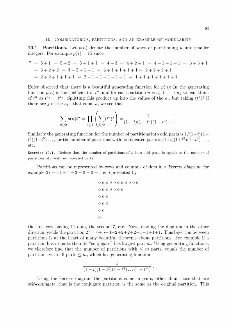
93

10. Combinatorics, partitions, and an example of modularity

10.1. Partitions. Let p(n) denote the number of ways of partitioning n into smallerintegers. For example p(7) = 15 since

7 = 6 + 1 = 5 + 2 = 5 + 1 + 1 = 4 + 3 = 4 + 2 + 1 = 4 + 1 + 1 + 1 = 3 + 3 + 1

= 3 + 2 + 2 = 3 + 2 + 1 + 1 = 3 + 1 + 1 + 1 + 1 = 2 + 2 + 2 + 1

= 2 + 2 + 1 + 1 + 1 = 2 + 1 + 1 + 1 + 1 + 1 = 1 + 1 + 1 + 1 + 1 + 1.

Euler observed that there is a beautiful generating function for p(n): In the generatingfunction p(n) is the coefficient of tn, and for each partition n = a1 + . . .+ ak we can thinkof tn as ta1 . . . tak . Splitting this product up into the values of the ai, but taking (ta)j ifthere are j of the ai’s that equal a, we see that

∑n≥0

p(n)tn =∏a≥1

∑j≥0

(ta)j

=1

(1− t)(1− t2)(1− t3) . . ..

Similarly the generating function for the number of partitions into odd parts is 1/(1−t)(1−t3)(1−t5) . . . , for the number of partitions with no repeated parts is (1+t)(1+t2)(1+t3) . . . ,etc.

Exercise 10.1. Deduce that the number of partitions of n into odd parts is equals to the number of

partitions of n with no repeated parts.

Partitions can be represented by rows and columns of dots in a Ferrers diagram; forexample 27 = 11 + 7 + 3 + 3 + 2 + 1 is represented by

o o o o o o o o o o o

o o o o o o o

o o o

o o o

o o

o

the first row having 11 dots, the second 7, etc. Now, reading the diagram in the otherdirection yields the partition 27 = 6+5+4+2+2+2+2+1+1+1+1. This bijection betweenpartitions is at the heart of many beautiful theorems about partitions. For example if apartition has m parts then its “conjugate” has largest part m. Using generating functions,we therefore find that the number of partitions with ≤ m parts, equals the number ofpartitions with all parts ≤ m, which has generating function

1

(1− t)(1− t2)(1− t3) . . . (1− tm).

Using the Ferrers diagram the partitions come in pairs, other than those that areself-conjugate; that is the conjugate partition is the same as the original partition. This

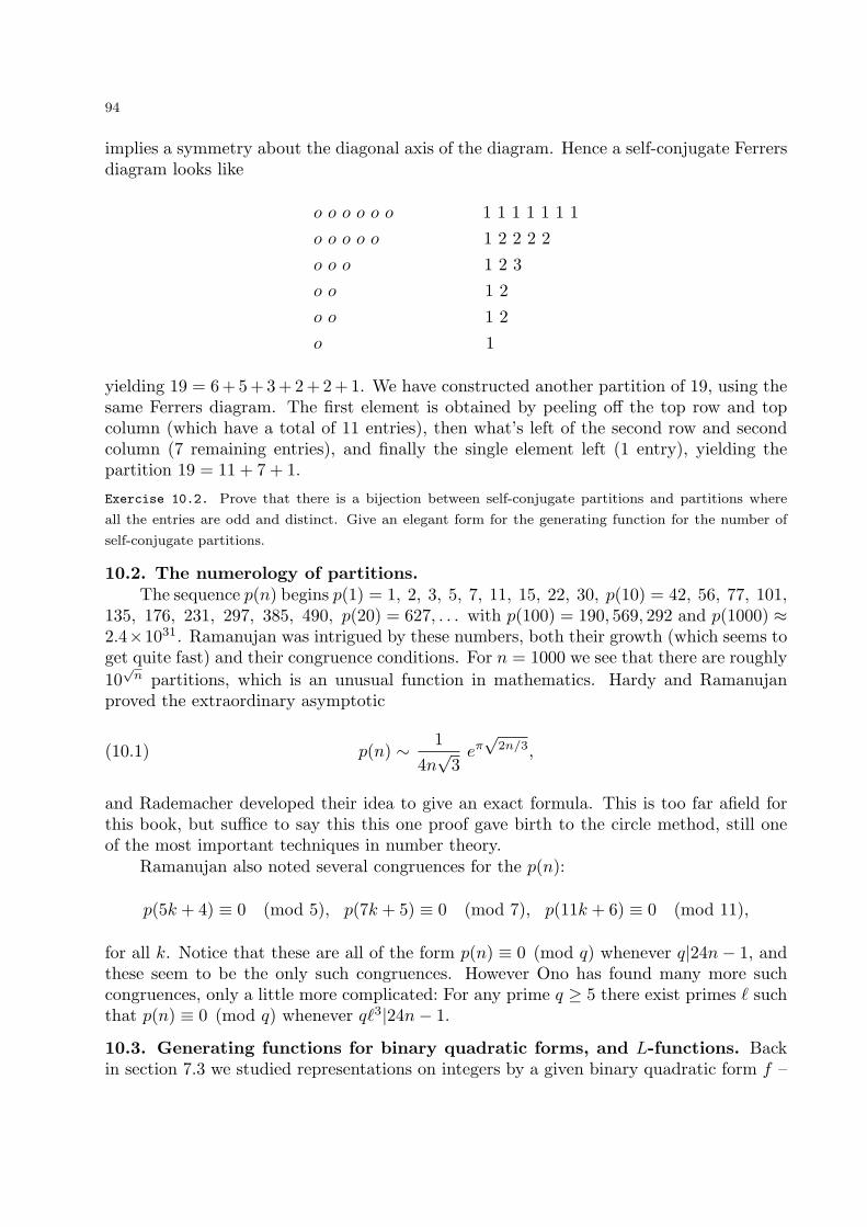
94

implies a symmetry about the diagonal axis of the diagram. Hence a self-conjugate Ferrersdiagram looks like

o o o o o o 1 1 1 1 1 1 1

o o o o o 1 2 2 2 2

o o o 1 2 3

o o 1 2

o o 1 2

o 1

yielding 19 = 6+5+3+2+2+1. We have constructed another partition of 19, using thesame Ferrers diagram. The first element is obtained by peeling off the top row and topcolumn (which have a total of 11 entries), then what’s left of the second row and secondcolumn (7 remaining entries), and finally the single element left (1 entry), yielding thepartition 19 = 11 + 7 + 1.

Exercise 10.2. Prove that there is a bijection between self-conjugate partitions and partitions where

all the entries are odd and distinct. Give an elegant form for the generating function for the number of

self-conjugate partitions.

10.2. The numerology of partitions.The sequence p(n) begins p(1) = 1, 2, 3, 5, 7, 11, 15, 22, 30, p(10) = 42, 56, 77, 101,

135, 176, 231, 297, 385, 490, p(20) = 627, . . . with p(100) = 190, 569, 292 and p(1000) ≈2.4×1031. Ramanujan was intrigued by these numbers, both their growth (which seems toget quite fast) and their congruence conditions. For n = 1000 we see that there are roughly

10√n partitions, which is an unusual function in mathematics. Hardy and Ramanujan

proved the extraordinary asymptotic

(10.1) p(n) ∼ 1

4n√3eπ√

2n/3,

and Rademacher developed their idea to give an exact formula. This is too far afield forthis book, but suffice to say this this one proof gave birth to the circle method, still oneof the most important techniques in number theory.

Ramanujan also noted several congruences for the p(n):

p(5k + 4) ≡ 0 (mod 5), p(7k + 5) ≡ 0 (mod 7), p(11k + 6) ≡ 0 (mod 11),

for all k. Notice that these are all of the form p(n) ≡ 0 (mod q) whenever q|24n− 1, andthese seem to be the only such congruences. However Ono has found many more suchcongruences, only a little more complicated: For any prime q ≥ 5 there exist primes ℓ suchthat p(n) ≡ 0 (mod q) whenever qℓ3|24n− 1.

10.3. Generating functions for binary quadratic forms, and L-functions. Backin section 7.3 we studied representations on integers by a given binary quadratic form f –

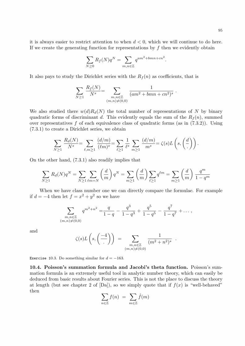
95

it is always easier to restrict attention to when d < 0, which we will continue to do here.If we create the generating function for representations by f then we evidently obtain∑

N≥0

Rf (N)qN =∑m,n∈Z

qam2+bmn+cn2

.

It also pays to study the Dirichlet series with the Rf (n) as coefficients, that is

∑N≥1

Rf (N)

Ns=

∑m,n∈Z

(m,n) =(0,0)

1

(am2 + bmn+ cn2)s.

We also studied there w(d)Rd(N) the total number of representations of N by binaryquadratic forms of discriminant d. This evidently equals the sum of the Rf (n), summedover representatives f of each equivalence class of quadratic forms (as in (7.3.2)). Using(7.3.1) to create a Dirichlet series, we obtain

∑N≥1

Rd(N)

Ns=∑ℓ,m≥1

(d/m)

(ℓm)s=∑ℓ≥1

1

ℓs

∑m≥1

(d/m)

ms= ζ(s)L

(s,

(d

.

)).

On the other hand, (7.3.1) also readily implies that

∑N≥1

Rd(N)qN =∑N≥1

∑ℓm=N

(d

m

)qN =

∑m≥1

(d

m

)∑ℓ≥1

qℓm =∑m≥1

(d

m

)qm

1− qm

When we have class number one we can directly compare the formulae. For exampleif d = −4 then let f = x2 + y2 so we have

∑m,n∈Z

(m,n)=(0,0)

qm2+n2

=q

1− q− q3

1− q3+

q5

1− q5− q7

1− q7+ . . . ,

and

ζ(s)L

(s,

(−4

.

))=

∑m,n∈Z

(m,n)=(0,0)

1

(m2 + n2)s.

Exercise 10.3. Do something similar for d = −163.

10.4. Poisson’s summation formula and Jacobi’s theta function. Poisson’s sum-mation formula is an extremely useful tool in analytic number theory, which can easily bededuced from basic results about Fourier series. This is not the place to discuss the theoryat length (but see chapter 2 of [Da]), so we simply quote that if f(x) is “well-behaved”then ∑

n∈Zf(n) =

∑m∈Z

f(m)

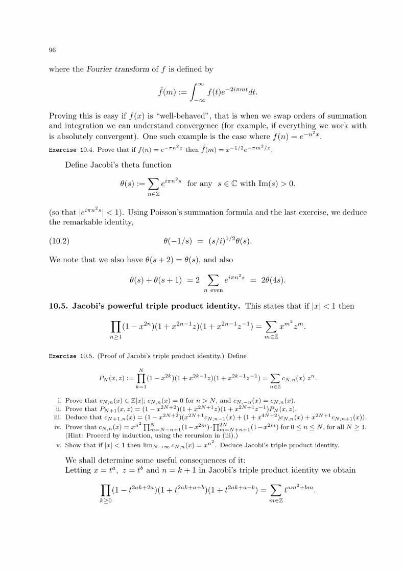
96

where the Fourier transform of f is defined by

f(m) :=

∫ ∞−∞

f(t)e−2iπmtdt.

Proving this is easy if f(x) is “well-behaved”, that is when we swap orders of summationand integration we can understand convergence (for example, if everything we work with

is absolutely convergent). One such example is the case where f(n) = e−n2x.

Exercise 10.4. Prove that if f(n) = e−πn2x then f(m) = x−1/2e−πm2/x.

Define Jacobi’s theta function

θ(s) :=∑n∈Z

eiπn2s for any s ∈ C with Im(s) > 0.

(so that |eiπn2s| < 1). Using Poisson’s summation formula and the last exercise, we deducethe remarkable identity,

(10.2) θ(−1/s) = (s/i)1/2θ(s).

We note that we also have θ(s+ 2) = θ(s), and also

θ(s) + θ(s+ 1) = 2∑n even

eiπn2s = 2θ(4s).

10.5. Jacobi’s powerful triple product identity. This states that if |x| < 1 then∏n≥1

(1− x2n)(1 + x2n−1z)(1 + x2n−1z−1) =∑m∈Z

xm2

zm.

Exercise 10.5. (Proof of Jacobi’s triple product identity.) Define

PN (x, z) :=N∏

k=1

(1− x2k)(1 + x2k−1z)(1 + x2k−1z−1) =∑n∈Z

cN,n(x) zn.

i. Prove that cN,n(x) ∈ Z[x]; cN,n(x) = 0 for n > N , and cN,−n(x) = cN,n(x).

ii. Prove that PN+1(x, z) = (1− x2N+2)(1 + x2N+1z)(1 + x2N+1z−1)PN (x, z).

iii. Deduce that cN+1,n(x) = (1− x2N+2)(x2N+1cN,n−1(x) + (1 + x4N+2)cN,n(x) + x2N+1cN,n+1(x)).

iv. Prove that cN,n(x) = xn2 ∏N

m=N−n+1(1−x2m) ·∏2N

m=N+n+1(1−x2m) for 0 ≤ n ≤ N , for all N ≥ 1.

(Hint: Proceed by induction, using the recursion in (iii).)

v. Show that if |x| < 1 then limN→∞ cN,n(x) = xn2. Deduce Jacobi’s triple product identity.

We shall determine some useful consequences of it:Letting x = ta, z = tb and n = k + 1 in Jacobi’s triple product identity we obtain∏

k≥0

(1− t2ak+2a)(1 + t2ak+a+b)(1 + t2ak+a−b) =∑m∈Z

tam2+bm.

97

Some special cases include a = 1, b = 0, yielding∏n≥1

(1− t2n)(1 + t2n−1)2 =∑m∈Z

tm2

;

and a = b = ± 12 , yielding ∏

k≥0

(1 + tk)(1− t2k+2) =∑m∈Z

tm2+m

2 .

Exercise 10.6. By writing 1 + tk as (1− t2k)/(1− tk) or otherwise, deduce that

∑m≥1

tm2+m

2 =(1− t2)(1− t4)(1− t6) . . .

(1− t)(1− t3)(1− t5) . . .

Letting x = ta, z = −tb and n = k + 1 in Jacobi’s triple product identity we obtain∏k≥0

(1− t2ak+2a)(1− t2ak+a+b)(1− t2ak+a−b) =∑m∈Z

(−1)mtam2+bm.

Some special cases include a = 1, b = 0, yielding∏n≥1

(1− tn)(1− t2n−1) =∑m∈Z

(−1)mtm2

;

and a =32 , b =

12 , yielding Euler’s identity,

∏n≥1

(1− tn) =∑m∈Z

(−1)mt3m2+m

2 .

Exercise 10.7. Interpret this combinatorially, in terms of the number of partitions of m into unequal

parts.

Exercise 10.8. If (12/.) is the Jacobi symbol, show that

t1/24∏n≥1

(1− tn) =∑m≥1

(12

m

)tm2

24 .

10.6. An example of modularity: y2 = x3 − x. Letting x = t4 and z = −1 in Jacobi’striple product identity we obtain∏

n≥1

(1− t8n)(1− t8n−4)2 =∑b∈Zb even

(−1)b/2tb2

.

98

Now letting x = t4 and z = −t4u in Jacobi’s triple product identity we obtain∏n≥1

(1− t8n)(1− αt8nu)(1− t8n−8/u) =∑m∈Z

t4m2+4m(−u)m.

In the product we change the exponent of the last term taking n in place of n − 1, andhence we have a left over term of 1 − 1/u. On the right side we pair up the term for mwith the term for −m− 1. Dividing through by 1− 1/u then yields

t∏n≥1

(1− t8n)(1− t8nu)(1− t8n/u) =∑m≥0

t4m2+4m+1(−1)m(um + um−1 + . . .+ u−m).

Taking u = 1 we obtain

t∏n≥1

(1− t8n)3 =∑a≥1a odd

(−1)a−12 ata

2

.

Multiplying these together yields

(10.3) t∏n≥1

(1− t4n)2(1− t8n)2 =∑

a,b∈Z, a≥1,a odd, b even

(−1)a+b−1

2 ata2+b2 =

∑n≥1

antn,

for certain integers an. In particular if p is a prime ≡ 3 (mod 4) then ap = 0; if p is a

prime ≡ 3 (mod 4) then writing p = a2 + b2 with a odd, we have ap = 2(−1)a+b−1

2 a.

Multiplicativity. We will show that the an are multiplicative: If odd n = rs with (r, s) =1 then the representations of n as the sum of two squares are given by the representationsof r = a2+b2 and s = A2+B2 where a,A are odd. This pair yields the two representations

rs = (aA+ bB)2 + (aB −Ab)2 = (aA− bB)2 + (aB +Ab)2.

These two representations contribute the following to the sum for ars:

2(−1)aA+bB+aB−Ab−1

2 (aA+ bB) + 2(−1)aA−bB+aB+Ab−1

2 (aA− bB) = 4(−1)aA+B+b−1

2 aA

= 2(−1)a+b−1

2 a · 2(−1)A+B−1

2 A,

since aA+bB+aB−Ab−12 ≡aA−bB+aB+Ab−1

2 ≡aA+B+b−12 ≡ A· a+b−12 + A+B−1

2 ≡a+b−12 + A+B−1

2(mod 2). Summing these up we do deduce that

ars = aras if (r, s) = 1.

99

At the prime powers. If p ≡ 1 (mod 4) then we can factor p = ππ in Z[i] for someprime π = a + bi. The possible factorizations of pk are ττ where τ = πjπk−j , eachfactorization counted twice. Now each πjπk−j is counted twice by the sets πiπk−1−i × πand πiπk−1−i × π, except πk and πk which are each counted once. Also each πjπk−j iscounted twice by πiπk−2−i × p. Using the calculation from the previous subsection, wededuce that

apk = apapk−1 − papk−2 .

This implies that(1− ap

ps+

p

p2s

)∑k≥0

apk

pks= 1+

apps

− apps

+∑k≥2

apk − apapk−1 + papk−2

pks= 1.

If p ≡ 3 (mod 4) then the only representations of pk as a sum of two squares are(pk/2)2 + 02 when k is even. Now (pk/2 − 1)/2 ≡ k/2 (mod 2) and so apk = 0 if k is odd,

and apk = (−p)k/2 is k is even. This implies, taking k = 2j, that(1+

p

p2s

)∑k≥0

apk

pks= 1 +

∑j≥1

(−p)j + (−p)j−1

p2js= 1.

Finally, for p = 2, we have no representation of 2k = a2 + b2 with a odd and b even.

Modularity. Combining the information in the last two subsections, since an is multi-plicative and we know the Euler factor at each prime, we deduce that

∑n≥1

anns

=∏

p primep odd

(1− ap

ps+

p

p2s

)−1

where ap is as above (though note that ap = 0 if p ≡ 3 (mod 4)). We see that the powerseries can be created by working only with the ap. Notice that in the Euler product we

have the usual Euler product term(1− ap

ps + pp2s

)−1, except for the exceptional prime 2.

Earlier in the course we proved that for the elliptic curve E : y2 = x3 − x if welet #E(Fp) = p + 1 − ap then ap = 0 if p ≡ 3 (mod 4) and, if p ≡ 1 (mod 4), we writep = a2 + b2 where a is odd and then

ap = 2(−1)a+b−1

2 a.

That is we get exactly the same values as above. Notice also that there is one exceptionalprime, 2, which is the only prime that divides the discriminant of y2 = x3 − x (and thediscriminant of the quadratic form x2 + y2). Could this all be a wild co-incidence?

100

11. Degree three curves — why the curve y2 = x3 + ax + b?

11.1. Parametric families of rational points on curves. We have seen that if alinear curve has infinitely many rational points then they can be parametrized (that is,they are given by a formula which is a linear polynomial in some unknown t). Indeedstarting from one given solution to ax0 + by0 = c we then have the parametric familyx = x0 + bt, y = y0 − at for any integer t.

We saw that we can proceed similarly for quadratics, given one solution we can param-etrize infinitely many others: To see this start by suppose that a, b, c are given non-zerointegers for which a + b + c = 0. One can check that if r, s, t are integers for whichr + s+ t = 0 then

a(bs2 + ct2)2 + b(as2 + cr2)2 + c(at2 + br2)2 = 0

This can be applied to show that any quadratic equation Ax2 + By2 = Cz2 with onenon-zero integral point has infinitely many given as polynomials in r, s, t. To do so simplyselect a = Ax2, b = By2, c = −Cz2 above and we obtain AX2 +BY 2 = CZ2 with

X = x(B(ys)2 − C(zt)2), Y = y(A(xs)2 − C(zr)2), Z = z(A(xt)2 +B(yr)2).

For example, for the equation x2 + y2 = 2z2 starting from the solution (1, 1, 1) weobtain the parametrization X = s2−2t2, Y = s2−2r2, Z = t2+r2, which we can re-write,taking t = −s− r, as −X = 2r2 + 4rs+ s2, Y = s2 − 2r2, Z = 2r2 + 2rs+ s2. Hence wesee that any quadratic with one solution has infinitely many given parametrically.

How about cubics or higher degree? We will show that there are no coprime, non-constant polynomials x(t), y(t), z(t) for which ax(t)3 + by(t)3 + cz(t)3 = 0, as a corollaryof a much more general result:

The abc Theorem for Polynomials. If a(t), b(t), c(t) ∈ C[t] do not have any commonroots and provide a genuine polynomial solution to a(t) + b(t) = c(t), then the maximumof the degrees of a(t), b(t), c(t) is less than the number of distinct roots of a(t)b(t)c(t) = 0.

This is a “best possible” result in that we can find infinitely many examples wherethere is exactly one more zero of a(t)b(t)c(t) = 0 than the largest of the degrees. Forexample the familiar identity (2t)2 + (t2 − 1)2 = (t2 + 1)2; or the rather less interestingtn + 1 = (tn + 1).

Corollary 11.1. There do not exist coprime, non-constant polynomials x(t), y(t), z(t) forwhich ax(t)3 + by(t)3 + cz(t)3 = 0.

Proof. Suppose that ax(t)3 + by(t)3 + cz(t)3 = 0 with a, b, c ∈ C where x(t), y(t), z(t)have no common roots and let a(t) = ax(t)3, b(t) = by(t)3, c(t) = cz(t)3. Let d be themaximum of the degrees of x(t), y(t), z(t). By the abc Theorem for Polynomials we knowthat 3d is less than the number of distinct roots of x(t)y(t)z(t) = 0, which is ≤ 3d, andhence we have a contradiction.

Proof of the abc Theorem for Polynomials. We differentiate a+b = c to obtain a′+b′ = c′.Now, define

∆(t) :=

∣∣∣∣ a(t) b(t)a′(t) b′(t)

∣∣∣∣ .

101

Note that ∆(t) = 0, else ab′ − a′b = 0 so that a′/a = b′/b and integrating implies that b isa scalar multiple of a, which contradicts hypothesis.

Let α be a root of a(t), and suppose (t − α)e is the highest power of (t − α) whichdivides a(t). Evidently (t− α)e−1 is the highest power of (t− α) which divides a′(t), andthus it is the highest power of (t − α) which divides ∆(t) = a(t)b′(t) − a′(t)b(t), since αis not a root of b(t). Therefore (t− α)e divides ∆(t)(t− α). Multiplying all such (t− α)e

together we obtain

a(t) divides ∆(t)∏

a(α)=0

(t− α).

An analogous argument works for b(t), and for c(t) since by adding the first column to thesecond in the definition of ∆(t), we obtain

∆(t) =

∣∣∣∣ a(t) c(t)a′(t) c′(t)

∣∣∣∣ .Hence, multiplying these together we obtain that

a(t)b(t)c(t) divides ∆(t)∏

(abc)(α)=0

(t− α).

The result follows by taking the degrees of both sides and noting that, by definition,

deg(∆) ≤ mindeg(a) + deg(b), deg(a) + deg(c), deg(c) + deg(b) − 1.

11.2. Constructing new rational points on cubic curves from old ones.

Let us suppose that f(x, y) ∈ Q[x, y] of degree 3.16 We wish to study rational points onthe curve

f(x, y) = 0.

If P = (u, v) is a rational point on f(x, y) = 0 we mean that f(u, v) = 0 and we sometimeswrite f(P ) = 0. We also let x(P ) := u and y(P ) := v, the x- and y-coordinates of P . Wesuppose that we are given two rational points P1, P2 on f(x, y) = 0. The equation of theline between them has rational coefficients, say y = λx+ τ .

Now if any point is on both the line and the curve then its coordinates satisfy

f(x, y) = 0 and y = λx+ τ,

so that F (x) := f(x, λx+τ) = 0. This is typically a polynomial of degree ≤ 3 with rationalcoefficients, in which case we can write F (x) = ax3 + bx2 + cx+ d where a, b, c, d ∈ Q. Weknow that this has roots x1 = x(P1) and x2 = x(P2). Moreover the sum of the roots of apolynomial F of degree 3 is given by −b/a and so the third root of F equals −b/a−x1−x2,

16That is, f is a polynomial of degree at most 3 in x and y (that is each term in the polynomial takesthe form ai,jx

iyj with i+ j ≤ 3 and = 3 for some non-zero ai,j , and the coefficients are rational numbers.

102

which we will call x3, another rational number. But then the point P3 = (x3, y3), wherey3 = λx3 + τ , is also on the curve f(x, y) = 0 and the line y = λx+ τ .

This is a beautiful way to construct new rational points on f(x, y) = 0 from givenones, and if we start with three non-collinear rational points on f(x, y) = 0 then we cantypically generate infinitely many in this fashion. However it would be preferable to startthis process with fewer points.

If we study the proof above then the key idea is that we need two rational points ona line with rational coefficients to generate a third point. The trick (spotted by Sir IsaacNewton) is to select the tangent line at a given rational point, in which case the tangentline has rational coefficients, and hence the third point at which the tangent line meets thecurve is also a rational point. Let’s study this more precisely: If the original rational pointis at (u, v) make the change of variable x → x + u, y → y + v so that we have f(P ) = 0with P = (0, 0). Then

∂f

∂y· dydx

+∂f

∂x=df(x, y)

dx= 0

and so if r =∂f∂y (P ) and s =∂f

∂x (P ) (which are rational numbers by substitution) then

the tangent line at P has equation ry + sx = 0. The tangent line is well-defined except ifr = s = 0.17 We therefore have a third rational point of intersection (of the curve and thetangent line), which we denote by P2. Using this point we create P3, P4, . . . . With a bitof luck these will all be distinct and there will therefore be infinitely many rational pointson the original cubic curve.

So if we are given a cubic curve with one rational point then we wish to study whetherthere are infinitely many rational points on the curve. It is difficult to attack this ques-tion directly because there are 10 coefficients of any arbitrary degree three polynomial intwo variables. As with quadratics we seek to reduce that number, since there are many“models” for any given curve, which can be obtained through rational transformations ofthe co-ordinates. In the next section we will see, given that there is a rational point onthe curve, we can reduce the number of variables in our general model to two.

11.3. Cubic curves into Weierstrass form. Suppose that we are given a curve C :f(x, y) = 0 of degree 3 with a rational point P , that is not a point of inflexion.18 Our goalis to show that either the curve can be parametrized,19 or the curve can be “re-written”as

(11.1) y2 = x3 + ax+ b,

with a rational point in the xy-plane, where a and b are integers with ∆ := 4a3+27b2 = 0,and there does not exist a prime p for which p4|a and p6|b. By “re-written” we mean thatthere is, more-or-less, a 1-1 correspondence between rational points on both curves, andwe can easily classify where there is not.

17In which case all of the monomials in f have degree 3. If we now change variables x→ x/z, y → 1/zand multiply through by z3, then we have an equation that is linear in z, and hence easily solved in rationals.

18P is a point of inflexion for C if the tangent at P only intersects C at P ; that is there is no other

point of intersection.19That is we can find a solution for x, y as functions of single variable.

103

Now draw the tangent to C at the point P1 := P = (x1, y1) and find a second rationalpoint P2 = (x2, y2) on C. These points are distinct, since P is not a point of inflexion.We make the change of co-ordinates x → (x2 − x1)x + x1, y → (y1 − y2)y + y2 to geta new equation for the curve with rational points at P1 = (0, 1), P2 = (1, 0). If wenow write the curve in homogenous form and map z → z + x + y then we have a curvez3+f1(x, y)z

2+f2(x, y)z+f3(x, y) = 0 (with each fj homogenous of degree j) and rationalpoints at P1 = (0, 1, 0) and P2 = (1, 0, 0) so that f3(1, 0) = f3(0, 1) = 0. Moreover thetangent at P1 is the line between the points, namely z = 0. We can also do a calculationto find the slope of the tangent at P1 in, say, the (x, z)-plane: we differentiate to obtain

(3z2 + 2f1(x, 1)z + f2(x, 1))dz

dx+z3 + f ′1(x, 1)z

2 + f ′2(x, 1)z + f ′3(x, 1) = 0

We know that at P1 we have x = z = dzdx= 0 and hence f ′3(0, 1) = 0. Therefore f3(x, y) =

gx2y for some rational number g. We may take g = 1 else if g = 0 we have a quadraticin x, y, and if g = 0 we divide the whole equation through by g. Therefore our curve is ofthe form

x2y + ax2 + bxy + cy2 + dx+ ey + f = 0.

Now let y → y − a to obtain the form

x2y + bxy + cy2 + dx+ ey + f = 0.

Next multiply through by y and let X = xy to obtain

X2 + bXy + cy3 + dX + ey2 + fy = 0.

Mapping X → y and y → x this is an equation of the form

(11.2) ax3 + by2 + cxy + dx2 + ex+ fy + h = 0

with h = 0. That is there is a rational point at (0, 0).We now show that the general equation (11.2) may be reduced to the form (11.1) or

something simpler. We may assume that b = 0 else (11.2) is linear in y. If b = 0 thenby2 + cxy + fy = bY 2 − b((c/2b)x+ f/2b)2 where Y = y + (c/2b)x+ f/2b so we reduce toan equation of the form

Y 2 = ax3 + bx2 + cx+ k;

and if h = 0 the rational point is now at (0, f/2b). Letting X = x + b/3a to reduce tothe form Y 2 = aX3 + cX + d; if h = 0 the rational point is now at (−b/3a, f/2b). Nowwe multiply through by a2 and let v = aY, u = ax to obtain v2 = u3 + Cu + D. Nowwe multiply through by q6 and make the change of variable v = q3y, u = q2x to obtainy2 = x3+ q4Cx+ q6D. We select q to be that rational number for which q4C and q6D areintegers, and minimally so, and we obtain (11.1). We select q so that these integers areminimal in order that when we reduce (11.1) mod p it is non-degenerate if possible – note

104

that it is degenerate, that is two roots of the cubic are congruent mod p, if and only if pdivides the discriminant.20

Moreover if we began with a rational point then we had h = 0 and the rational point(0, 0) satisfying (11.2); and now the rational point (−bq2/3, aq3f/2b) satisfying (11.1).

We have just seen that we may change co-ordinates on (11.1) for which a→ q4a, b→q6b for some rational q, and there is a 1-to-1 correspondence of rational points. We wishto determine invariants of the elliptic curve, that is quantities that do not change undersuch changes of variable. We see that the ratio a3 : b2 is fixed under such a transformation,and hence any rational function of that ratio. For reasons that will become more apparentlater, we choose the following (linear) transformation of that ratio for our invariant: Thej-invariant of the elliptic curve E : y2 = x3 + ax+ b over C, is defined as

j(E) = 1728· a3

4a3 + 27b2.

Exercise 11.3.1. Prove that two elliptic curves with the same j-invariant are isomorphic over C, and in

fact, at most a degree 2 field extension of the field defined by the coefficients of the two elliptic curves.

Now 4a3(x3+ ax+ b) = (2ax+3b)2(ax− 3b)+∆(ax+ b) = 0, where ∆ := 4a3+27b2.Therefore if ∆ = 0, then either our curve is y2 = x3, or y2 = (x + 3b/2a)2(x − 3b/a) =X2(X − c) for c = 9b/2a. In the first case the solutions are parametrized by (t2, t3);in the second let z = y/X to obtain the curve z2 = X − c so our parametrization is(z2 + c, z(z2 + c)).

Exercise 11.3.2. Assume that there is a point of inflexion of C and that the curve cannot be parametrized.

Follow a similar procedure to above, to first move the point to (0, 0), then make the tangent line y = 0,

and then show that the equation of the curve becomes ey3 + (ax + b)y2 + (cx + d)y + x3 = 0, for some

rationals a, b, c, d, e, after a simple change of variable.

Exercise 11.3.3. Show that x3 = y(y − 1)(y − 2) has three inflexion points, at (0, 0), (0, 1) and (0, 2).

Exercise 11.3.4. Prove that the point at infinity on (11.1) is an inflexion point.

11.4. Diagonal cubic curves. If one has a rational point (x, y, z) on the diagonal cubic

(11.3) ax3 + by3 + cz3 = 0,

then one obtains a rational point on another diagonal cubic:

(11.4) X3 + Y 3 + dZ3 = 0.

20We seek the minimal (integer) discriminant over all isomorphic models of the elliptic curve. Thencep divides this discriminant if and only if the curve is isomorphic mod p to some curve of lower degree (asin section 9.6). Our techniques here work for all primes p > 3. However for p = 2 and 3 one has to take

into account different possible models of the elliptic curve (because, for example, we cannot “complete thesquare” when working mod 2, to remove certain monomials).

105

whereX = C3+6AC2+3A2C−A3, Y = A3+6CA2+3C2A−C3, Z = 3xyz(A2+AC+C2),with A = ax3, B = by3, C = cz3 and d = abc.21 Therefore we can focus on the case wherea = b = 1, c = d in (11.3). Note that this is not an invertible map but certainly if thereare no solutions to X3 + Y 3 + abcZ3 = 0 then there are none to ax3 + by3 + cz3 = 0.

Now, given a solution to (11.4) let X = u+v, Y = u−v to obtain 2u3+6uv2+dZ3 = 0.De-homogenize by dividing through by u3 and letting z = −Z/u, V = v/u to obtain2 + 6V 2 = dz3, and obtain (11.2), and hence (11.1), specifically

(11.5) y2 = x3 − 432d2

with y = 36dV, x = 6dz.

11.5. y2 equals a quartic with a rational point. We have already seen that solutionsto quartics are “equivalent” to solutions to cubics: We saw that

If x4 + y4 = z2 then v2 = u3 + u with (u, v) = (x2/y2, xz/y3).In the other direction one has that

If v2 = u3 + u then x4 + y4 = z2 with (x, y, z) = (u2 − 1, 2v, u4 + 6u2 + 1).

One can generalize this further:If x4 + bx2y2 + cy4 = z2 then v2 = u3 + bu2 + cu with (u, v) = (x2/y2, xz/y3), and in

other direction we take (x, y, z) = (u2 − c, 2v, u4 + 2bu3 + 6cu2 + 2bcu+ c2).

In general we will suppose that we have any curve of the form

(11.6) y2 = f(x) where f has degree 4, with a rational point (k, a),

and try to covert it into the form (11.1). If we make a change of variable x→ x− k, thatis letting g(x) = f(x+ k) then the rational point on y2 = g(x) where g has degree 4 is at(0, a), and so g(0) = a2, that is g(x) = ex4 + dx3 + cx2 + bx + a2. Now divide y2 = g(x)through by 1/x4 letting v = y/x2, u = 1/x (which has inverse x = 1/u, y = v/u2), sothat

(11.7) v2 = a2u4 + bu3 + cu2 + du+ e.

If a = 0 we have a cubic and have reduced to (11.2). If a = 0 then write h(u) = au2 +(b/2a)u+(c/2a− b2/4a3) (which we write as au2 +Bu+C) so that h(u)2 = a2u4 + bu3 +cu2 + . . . Therefore changing variable v = w + h(u) we obtain the equation

w2 + 2w(au2 +Bu+ C) = ℓu+m.

Now we multiply through by w and let t = uw to obtain

w3 + 2at2 + 2Btw + 2Cw2 = ℓt+mw,

and we have reduced to (11.2).

21The transformation from (11.3) to (11.4) can be obtained from the identity

(1− 6t+ 3t2 + t3)3 − (1 + 3t− 6t2 + t3)3 + t(t− 1)(3(t2 − t+ 1))3 = 0;

by substituting in t = −A/C, and multiplying through by C9.

106

11.6. The intersection of two quadratic polynomials in three variables (that is,the intersection of two quadratic surfaces). Here we have two quadratic polynomialsf, g in three variables, with no common factors, and for which

(11.8) f(x, y, z) = g(x, y, z) = 0 has the common rational point (x0, y0, z0).

By change of variable x→ x+x0, y → y+ y0, z → z+ z0 we may assume that the rationalpoint is at (0, 0, 0). We write f = f2 + f1 + f0 where fj is the sum of the monomialsof f of degree j. Then f0 = f(0, 0, 0) = 0. Hence we are studying the solutions tof2 + f1 = g2 + g1 = 0. Therefore f1g2 − g1f2 = 0 is a homogenous cubic on which therational points lie; de-homogenizing yields a cubic in two variables, and thus we are in thesituation above which we know can be reduced to (11.1), unless f1g2 − g1f2 is identicallyzero. But then either f1 = cg1 and f2 = cg2 so that f = cg; or f1|f2 and g1|g2, so thatf = f1h and g = g1h where h is a linear polynomial. Either way f and g have a commonfactor contradicting the hypothesis.

11.7. Doubling a point on a diagonal cubic. Doubling a point on a diagonal cu-bic involves several transformations, but it works out more elegantly to give the formuladirectly: If we have a solution to (11.3) then we take t = −A/C in the identity,

t(t− 2)3 + (1− t)(1 + t)3 + (2t− 1)3 = 0,

multiply through by C9, where A = ax3, B = by3, C = cz3 and take X = x(B − C), Y =y(C −A), Z = z(A−B) to obtain another solution to (11.3):

aX3 + bY 3 + cZ3 = A(B − C)3 +B(C −A)3 + C(A−B)3 = 0.

107

12. The rational points on an elliptic curve

12.1. The group of rational points on an elliptic curve. We have just seen how acubic with a rational point can be transformed to an equation of the affine form

E : y2 = x3 + ax+ b

with a, b ∈ Z by linear maps with rational coefficients. This is called an elliptic curve.We have seen that two rational points on the unit circle gave rise to a line with rationalcoefficients and vice-versa; this allowed us to find all the rational points on the unit circle.We extend that idea to elliptic curves. Let E(Q) denote all of the rational points on E(that is (x, y) on E with x, y ∈ Q).

Exercise 12.1.1. Show that if (x, y) ∈ E(Q) then there exist integers ℓ,m, n such that x = m/n2, y =

ℓ/n3 with (ℓm, n) = 1. Moreover the point at ∞ corresponds to n = 0, ℓ = m = 1.

Exercise 12.1.2. Let ∆ = 4a3 + 27b2. Show that if a > 0 or if ∆ > 0 then x3 + ax+ b = 0 has just one

real root. Show that if a,∆ < 0 then x3 + ax+ b = 0 has three real roots. Sketch the shape of the curve

y2 = x3 + ax+ b in the two cases.

Suppose that we are given two points (x1, y1), (x2, y2) ∈ E(Q). The line betweenthem, y = mx + ν has m, ν ∈ Q.22 These two points are both intersections of the liney = mx+ ν with the elliptic curve y2 = x3 + ax+ b, that is x1, x2 satisfy

(mx+ ν)2 = y2 = x3 + ax+ b;

in other words x1 and x2 are two of the three roots of the cubic polynomial

x3 −m2x2 + (a− 2mν)x+ (b− ν2) = 0.

If the third root is x3 then x3 = m2 − x1 − x2 ∈ Q and if we let y3 = mx3 + ν we obtainthe third intersection of the line with E, and (x3, y3) ∈ E(Q). This method of generatinga third rational point from two given ones goes back to Fermat.

Actually one can do even better and generate a second point from a given one: If(x1, y1) ∈ E(Q) let y = mx + ν be the equation of the tangent line to y2 = x3 + ax + bat (x1, y1). To calculate this simply differentiate to obtain 2y1m = 3x21 + a and thenν = y1 − mx1. Now our cubic polynomial has a double root at x = x1 and we againcompute a third point by taking x3 = m2 − 2x1, y3 = mx3 + ν so that (x3, y3) ∈ E(Q).

In these constructions we missed the case when the line is vertical (in the first casex1 = x2 which implies that y2 = −y1; in the second case y = 0). Where is the thirdpoint of intersection? One cannot see another point of intersection on the graph (that ison the real plane), but the line stretches to infinity, and indeed the third point is, rathersurprisingly, the point at infinity, which we denote 0. Remember from section C11, inprojective co-ordinates the elliptic curve is y2z = x3 + axz2 + bz3 so the point at infinityis (0, 1, 0).

22Or is of the form x = x1 = x2, a situation we will deal with a little later.

108

Exercise 12.1.3. Prove that there cannot be four points of E(Q) on the same line.

Poincare made an extraordinary observation: If we take any three points P,Q,R ofE on the same line then we can define a group by taking P + Q + R = 0. The lineat infinity tells us that the point at infinity is indeed the 0 of this group. Moreover wehave seen that (x, y) + (x,−y) = 0. Note that this implies that, in the notation above,(x3,−y3) = (x1, y1) + (x2, y2)

It is clear that the operation is closed under addition (and, most interestingly, closedin the subgroup E(Q)). The one thing that is complicated to justify is that Poincare’soperation (of addition) is indeed associative, and that hence we do indeed have a group.

Exercise 12.1.4. Show that the addition law given here is indeed associative. There are several proofs

of this fact. One method is to prove it purely geometrically, which is not easy (such proofs can be found in

most textbooks). Another proof involves find formulae for the co-ordinates of (P+Q)+R and P+(Q+R),

much as in 12.1.6, and verify that these are the same. This is tedious to implement, even using symbolic

algebra software. We will give a third, analytic, proof, later in section *.*. The advantage is that this

proof is quite elegant and follows from a body of essential theory.

It is also obvious that the addition law is commutative. The question then becomesto identify the structure of the group of rational points, E(Q).

Is E(Q) finite or infinite? Suppose that we have a rational point P . Take the tangent,find the third point of intersection of the tangent line with E to obtain −2P , and thenreflect in the x-axis to obtain 2P . Fermat suggested that if we repeat this process over andover again, then we are unlikely to come back again to the same point. If we never returnto the same point then we say that P has infinite order; otherwise P has finite order, theorder being the minimum positive integer n for which nP = 0 (points of finite order areknown as torsion points).

Exercise 12.1.5. Prove that the torsion points form a subgroup.

Exercise 12.1.6. Prove that if P = (x, y) with y = 0 then 2P = (X,Y ) where

X =(x2 − a)2 − 8bx

4y2, Y =

x6 + 5ax4 + 20bx3 − 5a2x2 − 4abx− 8b2 − a3

8y3.

Notice that the numerator and denominator of X are polynomials of degree four in x implying (roughly)

that the co-ordinates of 2P are about four times the length of the co-ordinates of P , unless there is

an enormous amount of cancelation between numerator and denominator. To express this better it is

convenient to define the height of P , H(P ) := max|m|, n2. Our observation is that H(2P ) ≈ H(P )4.

Exercise 12.1.7. Show that (x, y) has order 2 if and only if y = 0. Deduce that the number of points of

order 1 or 2 is one plus the number of integer roots of x3 + ax+ b; and therefore equals 1, 2 or 4.

12.2. The group law on the circle, as an elliptic curve. The points on the circlex2+y2 = 1 may be parametrized by Pθ := (cos θ, sin θ), where θ is taken mod 2π. Additionof points may be defined by Pθ+Pϕ = Pθ+ϕ, which yields an abelian group with P0 = (1, 0)as the identity. To show that this is a special case of the addition laws above we begin byhomogenizing to make this into the cubic curve

C : x2z + y2z = z3,

109

which has the affine points x2+y2 = 1, and all possible points (x, y, 0) at infinity. Any lineax+ by = c meets the circle x2+ y2 = 1 in two (complex) points (including multiplicities),and also meets C at infinity at the point (−b, a, 0). (In other words these are the projectivepoints on the intersection of ax+by = cz and x2+y2 = z2.) The line joining this to (1, 0, 1)is parallel to the original line and has equation ax + by = az; and so meets x2 + y2 = z2

again at (a2 − b2, 2ab, a2 + b2).We need to figure out how to add two points on this curve:

Doubling a point Pθ := (cos θ, sin θ) on x2 + y2 = 1, we note that 2y dydx +2x = 0 so that

the slope of the tangent line tθ :=dydx= − x

y= − cos θsin θ . As in the paragraph above, this line

meets C again at (cos θ,− sin θ, 0) = −2Pθ; and then drawing the line from −2Pθ to P0

the third point of intersection is

2Pθ = (cos2 θ − sin2 θ, 2 sin θ cos θ, sin2 θ + cos2 θ) = (cos 2θ, sin 2θ, 1) = P2θ,

as claimed.

Adding two distinct points: The line between Pθ and Pϕ has slope sin θ−sinϕcos θ−cosϕ= − cos( θ+ϕ

2 )

sin( θ+ϕ2 )

;

so proceeding as in the paragraph this meets C again at

−Pθ − Pϕ =

(cos(

θ + ϕ

2),− sin(

θ + ϕ

2), 0

)= −2P θ+ϕ

2= −Pθ+ϕ

and the result follows.

Since any conic can be transformed into the circle via line transforming transforma-tions, the same generalization of the elliptic curve group law holds true on any conic.

12.3. No non-trivial rational points by descent. There are some elliptic curves forwhich we can show that there are no rational points by an easy descent: Suppose thatx, y ∈ Q such that y2 = x3 + x, so that x = m/n2, y = ℓ/n3 with (ℓm, n) = 1 and

ℓ2 = m(m2 + n4).

Now (m,m2+n4) = (m,n4) = 1 so that both m and m2+n4 are squares, say m = u2 andm2 + n4 = w2. Therefore

n4 + u4 = m2 + n4 = w2,

and we showed, in section 6.4, that this has no non-trivial solutions. The trivial solutionshave either n = 0 (corresponding to the point O at ∞), or u = 0 (corresponding to thepoint (0, 0) of order two). Hence E(Q) ∼= Z/2Z.

12.4. The group of rational points of y2 = x3 − x. We will begin by applying theideas from elementary number theory to rational points on the elliptic curve

E : y2 = x3 − x.

110

We see that there are several rational points: the point at infinity, as well as the threepoints of order two, (−1, 0), (0, 0), (1, 0). Are there any others? By exercise 12.1.1 we canwrite x = m/n2, y = ℓ/n3 with (ℓm, n) = 1 to obtain

(m− n2)m(m+ n2) = ℓ2.

Here we have that the product of three integers equals a square, so we can write each ofthem as a squarefree integer times a square, where the product of the three squarefreeintegers must also equal a square. Note that the three squarefree integers cannot have acommon factor, else that factor cubed is a square and so the integers were not squarefree.This means that we can write

m− n2 = pqu2, m = prv2, m+ n2 = qrw2,

for some squarefree integers p, q, r which are pairwise coprime. Moreover since the productof the integers is positive, and as m−n2 < m < m+n2 we see that m+n2 > 0 and m−n2and m have the same sign. Hence we may assume that p has the same sign as m, and qand r are positive. Now note that (m±n2,m) = (n2,m) = 1 and so |p| = r = 1. Moreover(m − n2,m + n2) = (m − n2, 2n2) = (m − n2, 2) since (m − n2, n2) = (m,n2) = 1. Tosummarize, we have proved that there are four possibilities for the value of (p, q, r), sincep = −1 or 1 and q = 1 or 2. That leads to four sets of equations:

m− n2 = u2∣∣ m− n2 = −u2

∣∣ m− n2 = 2u2∣∣ m− n2 = −2u2

m = v2∣∣ m = −v2

∣∣ m = v2∣∣ m = −v2

m+ n2 = w2∣∣ m+ n2 = w2

∣∣ m+ n2 = 2w2∣∣ m+ n2 = 2w2

Note that these four cases do each have a solution with (m,n) = (1, 0), (0, 1), (1, 1), (−1, 1),respectively, which correspond to the four rational points O, (0, 0), (1, 0), (−1, 0), respec-tively, that we already know.

Let us suppose that we have another rational point on the curve P = (m/n2, ℓ/n3), sothat we have four new rational points, P = P+O, P+(0, 0), P+(1, 0) and P+(−1, 0). Wenow show that if P gives rise to a solution to the second set of quadratic equations, thenP +(0, 0) gives rise to a solution to the first set of quadratic equations (and, analogously, ifP gives rise to a solution to the third or fourth set of quadratic equations, then P + (1, 0)or P + (−1, 0), respectively gives rise to a solution to the first set of quadratic equations):

The line between P and (0, 0) is mny = ℓx. If P +(0, 0) = (u, v) then u+m/n2+0 =(ℓ/mn)2, so that u = (ℓ2 −m3)/m2n2 = −n2/m. since ℓ2 = m3 −mn4. Hence we see thatm and n2 in the first equations must be replaced by n2 and −m respectively, so that thethree equations yield n2 +m = w2, n2, n2 −m = u2, respectively, as claimed.

Exercise 12.4.1. Show that if P gives rise to a solution to the third or fourth set of quadratic equations,

then P + (1, 0) or P + (−1, 0), respectively gives rise to a solution to the first set of quadratic equations.

Hence we have now proved that for any P ∈ E(Q), at least one of P, P+(0, 0), P+(1, 0)and P + (−1, 0) gives rise to a solution in coprime integers (m,n) to m − n2 = u2, m =v2, m + n2 = w2. Substituting in m = v2 yields that v2 − n2 = u2, v2 + n2 = w2, andmultiplying these together yields a solution to

X4 − Y 4 = z2 with (X,Y ) = 1 and X + Y odd.

111

(Our solution is (v, n, uw); since v2 = m we have (v, n) = 1; since v2 + n2 = w2 with(v, n) = 1 we know that they have opposite parity.) We will show that this has no non-trivial solution, by a Fermat-type descent argument. If there are solutions then we knowfrom the Pythagorean equation z2 + (Y 2)2 = (X2)2 in coprime integers that there existcoprime integers r, s of different parity such that X2 = r2 + s2 and Y 2 = 2rs (as X,Y areof different parity). Now (r,X)|(Y 2, X) = 1, and so there exist coprime positive integersp, q of different parity such that r = 2pq, s = p2 − q2. Therefore 4pq(p2 − q2) = 2rs = Y 2.Since p, q, p2 − q2 are positive and coprime we obtain that they are each squares, sayx2, y2, z2 and so x4 − y4 = z2.

Exercise 12.4.2. Show that x, y, z is a “smaller” solution that X,Y, Z and therefore complete the proof.

The challenge here is to define the size of a solution in such a way that the argument here works smoothly.

From all this we deduce that E(Q) = O, (0, 0), (1, 0), (−1, 0).

Our goal in the next few sections is to generalize this proof to more elliptic curves.Let’s rephrase the argument in a way that makes sense to generalize: We will suppose thatE : y2 = x3 + ax + b = (x − r1)(x − r2)(x − r3) where, for now, r1, r2, r3 are integers,though eventually we will have to consider the case where x3 + ax+ b is irreducible.

Step One: Define a map ϕ : E(Q) → Q3 where ϕ(P ) = (x − r1, x − r2, x − r3). Weknow that the three co-ordinates are rational numbers whose product is a square, and weclassified the three numbers by writing them as a squarefree integer times a square. Nowthe three squarefree numbers have product that is a square, even in the case that one ofx− r1, x− r2, x− r3 equals 0. So we could instead define

ϕ : E(Q) → (a, b, c) : a, b, c ∈ (Q∗/(Q∗)2)3 and abc = 1.

Step Two: We observed that we can write a = pq, b = rp, c = qr where p, q and r aresquarefree divisors of r1 − r2, r1 − r3 and r3 − r2 respectively. Moreover if r1 > r2 > r3then x−r3 > 0 and so we can assume that q and r are positive, and that p may be positiveor negative. These conditions imply that

ϕ(E(Q)) ⊂ (p, q, r) : p|r1 − r2, q|r1 − r3 r|r3 − r2, and q, r ≥ 1.

and so ϕ(E(Q)) is finite.

Step Three: For each element v ∈ ϕ(E(Q)) fix some Pv ∈ E(Q) for which ϕ(Pv) = v.Given any element P ∈ E(Q), suppose that v = ϕ(P ). The key new idea in our constructionabove, was that ϕ(P + Pv) = (1, 1, 1).

Step Four: Find a descent argument. That is, given a point P ∈ ϕ(E(Q)), for whichϕ(P ) = (1, 1, 1), show that there is a “smaller” point R ∈ ϕ(E(Q)), for which ϕ(R) =(1, 1, 1).

This is a lot to ask for! Particularly since it cannot always end up in a contradictionas there are elliptic curves with infinitely many rational points. To pursue this argumentwe will need to better understand torsion points, the map ϕ, and to find a precise notionof the size of a solution.

112

12.5. The arithmetic of a torsion point. Elizabeth Lutz and Nagell showed thatthere are only finitely many torsion points in E(Q). To be more precise they proved:

The Lutz-Nagell Theorem. If (x, y) ∈ E(Q) is a point of order m > 1 then(i) If m = 2 then y = 0 and x is an integer;(ii) If m > 2 then x and y are integers, and y2 divides ∆ = 4a3 + 27b2.Therefore there are only finitely many torsion points in E(Q).

The key idea in the proof is to show that if x(P ) = m/n2 with (m,n) = 1 and n > 1then x(kP ) = M/N2 with (M,N) = 1 and N divisible by n. An immediate consequenceof this is that if P = (x, y) is a torsion point then x is an integer, and hence y is an integer.

Proof of the easy parts of the theorem. (i) We see that 2P = 0 if and only if −P = P . Soif P = (x, y) then y = −y so that y = 0 and hence x is an integer.

For the final part of the theorem, note that if P = (x, y) is a torsion point, that ismP =0 for somem > 2 thenm·(2P ) = 2·nP = 0 so 2P = (X,Y ) is also a torsion point, and hencex, y,X, Y are all integers. Now m2 = 2x+X ∈ Z so that m = (3x2+a)/2y ∈ Z; that is 2ydivides 3x2+a. Hence y divides 9(3b−2ax)(x3+ax+b)+(6ax2−9bx+4a2)(3x2+a) = ∆.Since there are only finitely many divisors y of 4a3 +27b2, and each such y gives rise to atmost three values of x, hence there are only finitely many torsion points in E(Q). Actuallywe can better than this: Since 2P is also a torsion point, x(2P ) = ((x2 − a)2 − 8bx)/4y2 isan integer. In particular this implies that y2 equals x3+ax+ b and divides (x2−a)2−8bxso that it must also divide

(12.1) (3x2 + 4a)((x2 − a)2 − 8bx)− (x3 + ax+ b)(3x3 − 5ax− 27b) = 4a3 + 27b2.

Exercise 12.5.1. Prove that P has finite order if and only if there exists i > j ≥ 0 such that 2iP = ±2jP .

Mazur improved the Lutz-Nagell theorem showing that the torsion subgroup of E(Q)contains at most 16 points. In fact this subgroup is either Z/NZ for some 1 ≤ N ≤ 10or N = 12, or it is Z/2Z × Z/2NZ for some 1 ≤ N ≤ 4. After Mazur’s Theorem it isnot difficult to identify torsion points. First determine all integers y for which y2 divides4a3 + 27b2, and then compute all such points (x, y) ∈ E(Q).

Exercise 12.5.2. Show that P ∈ E(Q) has finite order if and only if x(P ), x(2P ), x(4P ), x(8P ),∞ are not

distinct.

There can be torsion points in fields other than Q. One can ask for them in C; infact their x-co-ordinates are roots of a polynomial with integer coefficients, so they arealgebraic numbers. We will show later that the subgroup of torsion points of order N isisomorphic to Z/NZ×Z/NZ for each N ≥ 1, so that there are N2 points of order dividingN .

Exercise 12.5.3. Prove that there are exactly N2∏

p|N (1− 1p2

) points of order N on E(C).

We will need the following lifting lemma, which generalizes the result in exercise 8.3.3,explaining how the orders of points modulo different powers of p are related:

113

Lemma 12.0. Suppose that P = (x, y) ∈ E(Q) with x = m/n2, y = ℓ/n3, where ℓ,mand n = n(P ) are integers for which (ℓm, n) = 1 (as in exercise 12.1.1). If p is a primefor which pk∥n(P ) with k ≥ 1 then pk+ℓ∥n(rpℓP ) for any ℓ ≥ 0 where p |r.

Deduction of the Lutz-Nagell Theorem. Suppose that P = (x, y) is a torsion point of E,but not O, so that there exists an integer s > 1 for which sP = 0. If x = m/n2 with n ≥ 1(as in exercise 12.1.1), and p is a prime for which pk∥n(P ) with k ≥ 1, then pk+ℓ∥n(sP )where s = rpℓ and p |r, by Lemma 12.0. However this is incompatible with the fact thatn(sP ) = 0. Hence n cannot be divisible by any prime p, so that n = 1; that is x, and soy, are integers.

Proof of Lemma 12.0. To understand better the exact power of a prime p dividing n, itmakes sense to study x/y = mn/ℓ. Hence we make the change of variable u = x/y, v = 1/y(which has inverse x = u/v, y = 1/v so is 1-to-1), so we have the equation

v = y2/y3 = (x/y)3 + a(x/y)(1/y) + b/y3 = u3 + auv2 + bv3.

Note that the map x→ x, y → −y can be realized as the map u→ −u, v → −v, so thatif P = (u, v) then −P = (−u,−v).Exercise 12.5.4. Prove that if n ≡ 0 (mod q) then u ≡ 0 (mod q) and v ≡ 0 (mod q3).

Given two distinct points Pi := (ui, vi), i = 1, 2 with ni ≡ 0 (mod q) we determineP1 + P2 = (u3, v3): To begin with we have

v1 − v2 = u31 − u32 + au1v21 − au2v

22 + bv31 − bv32

= (u31 − u32) + a(u1 − u2)v21 + au2(v

21 − v22) + b(v31 − v32),

so that the slope of the line between P1 and P2 is

λ :=v2 − v1u2 − u1

=(u21 + u1u2 + u22) + av21

1− au2(v1 + v2)− b(v21 + v1v2 + v22)≡ 0 (mod q2).

Exercise 12.5.5. Argue (by continuity) that if P1 = P2 then λ = (3u2 + av2)/(1− 2auv − 2bv2).

If the line between P1 and P2 has equation v = λu + τ then τ = v1 − λu1 ≡ 0 (mod q3).If we substitute the equation of the line into the equation for the curve we obtain that

λu+ τ = u3 + au(λu+ τ)2 + b(λu+ τ)3

a cubic equation whose roots are u1, u2 and −u3. Hence

u1 + u2 − u3 = − 2aλτ + 3bλ2τ

1 + aλ2 + bλ3≡ 0 (mod q5).

With this tool in hand we proceed with an exercise:

Exercise 12.5.6. (i) Show that if P ∈ E(Q) then u(mP ) ≡ mu(P ) (mod n(P )5) for all m ≥ 1.

(ii) Deduce that if p is a prime and pk∥n(P ) with k ≥ 1 then pk+ℓ∥n(mP ) where pℓ∥m. (Hint: Apply (i)

for P, pP, p2P, . . . in place of P .)

114

So now suppose that P = (x, y) is a torsion point of E, so that there exists an integerm for which mP = 0. If x = m/n2 and p is a prime for which pk∥n(P ) with k ≥ 1, thenpk+ℓ∥n(mP ). However this is incompatible with the fact that n(mP ) = 0. Hence p cannotdivide n for every prime p, so that n = 1; that is x and y are integers.

Example: Torsion on Ea : y2 = x3 + ax where 4 |a: We see that Ea has the point (0, 0)of order 2 and no other, unless a = −b2 for some odd b, in which case there are also(−b, 0) and (b, 0). We shall now show that there are no other torsion points: Suppose thatP = (x, y) ∈ E(Q) has order > 2. By Nagell-Lutz, both x and y are integers and y2|4a3.Now x(2P ) = (x2 − a)/2y and so 2|x2 − a. Therefore y2 = x3 + ax = x(x2 − a) + 2ax ≡ 0(mod 2), and thus 2|y and hence 4|x2 − a. Therefore a is odd else 2|x which implies 4|a,a contradiction. Therefore x is odd and a ≡ x2 ≡ 1 (mod 4), and so 0 ≡ y2 = x3 + ax ≡x(x2 + 1) ≡ 2 (mod 4), a contradiction.

Exercise 12.5.7. Using the Nagell-Lutz Theorem and Mazur’s theorem, determine the torsion subgroupfor each of the following curves:

i. y2 = x3 − 2, which has ∆ = 2233

ii. y2 = x3 + 8, which has ∆ = 2633

iii. y2 = x3 + 4 which has ∆ = 2433

iv. y2 = x3 + 4x which has ∆ = 28

v. y2 − y = x3 − x2 (or y2 = x3 − 432x+ 8208) which has ∆ = 2831211vi. y2 = x3 + 1, which has ∆ = 33

vii. y2 = x3 − 43x+ 166 which has ∆ = 21513

viii. y2 + 7xy = x3 + 16x (or y2 = (x− 147)(x2 + 147x− 22482)) which has ∆ = −21631617ix. y2 + xy + y = x3 − x2 − 14x+ 29 (or y2 = x3 − 219x+ 1654) which has ∆ = 217315

x. y2 + xy = x3 − 45x+ 81 (or y2 = (x− 75)(x2 + 75x− 52722)) which has ∆ = −21831711xii. y2 + 43xy − 210y = x3 − 210x2 (or y2 = (x − 3531)(x2 + 3531x − 20871666)) which has ∆ =

−220318537413ii.ii. y2 = x(x− 2)(x+ 2), which has ∆ = −28

ii.iv. y2 + xy − 5y = x3 − 5x2 (or y2 = (x− 21)(x− 102)(x+ 123)) which has ∆ = −2831654

ii.vi. y2 + 5xy − 6y = x3 − 3x2 (or y2 = (x− 66)(x− 111)(x+ 177)) which has ∆ = −21031852

ii.viii. y2 +17xy− 120y = x3 − 60x2 (or y2 = (x− 282)(x− 1011)(x+1293)) which has ∆ = −2163205472

12.6. Embedding torsion in Fp. We are interested in how the torsion subgroupTors(E(Q)) “reduces” mod p. It is easiest to study those primes p for which p |∆ since thenx3+ax+b has no repeated roots mod p, and so the reduction map ρp : E(Q) → E(Z/pZ) is ahomomorphism. Now if P = Q ∈ E(Q) but ρp(P ) = ρp(Q), then if R = P−Q ∈ E(Q)\Owe have ρp(R) = 0. But this implies that if R = (m/n2, ℓ/n3) with (ℓm, n) = 1 then p|n.However, the Lutz-Nagell theorem tells us that if R ∈ Tors(E(Q)) then n = 1 and so pcannot divide n. Hence we see that

ρp : Tors(E(Q)) → E(Z/pZ), is an injection.

This implies, since E(Z/pZ) is ∼= E(Fp) :Theorem 12.1. If prime p |∆E then E(Fp) contains a subgroup which is isomorphic toTors(E(Q)).

This provides a useful way of bounding the possibilities for torsion, since we simplyneed to compute ∆, find the smallest prime (or primes) that does not divide ∆, deter-mine the structure of E(Fp) and we know that this contains (as an abstract group), theTors(E(Q)).

115

12.7. The growth of points. In exercise 12.1.6 we saw that if P = (m/n2, ℓ/n3) with(ℓm, n) = 1 then

x(2P ) =(m2 − an4)2 − 8bmn6

4n2(m3 + amn4 + bn6).

The numerator and denominator of x(2P ) are each polynomials of degree four in m andn2, so we expect 2P to have co-ordinates about four times as long as those of P . Wewant to make this intuition precise. For a given rational number r/s with (r, s) = 1we define its height to be H(r/s) = max|r|, |s|. We extend this to points on E bytaking H(P ) = H(x(P )). Hence H(P ) = max|m|, n2, and so H(O) = 1. We believethat H(2P ) is around H(P )4. The main difficulty is that to determine H(2P ), we mustfirst divide the numerator and denominator of x(2P ) = R/S by (R,S). Now (n,R) =(n, (m2 − an4)2 − 8bmn6) = (n,m4) = 1. Moreover (m3 + amn4 + bn6, R) divides

(12.2) (3m2 + 4an4)R− (m3 + amn4 + bn6)(3m3 − 5amn4 − 27bn6) = ∆n12

by (12.1), and hence it divides ∆ as (R,n) = 1. We deduce that (R,S) divides 4∆,23 andso max|R|, |S|/4∆ ≤ H(2P ) ≤ max|R|, |S|. Now as |m|, n2 ≤ H(P ) we see that

|R| ≤ ((1 + |a|)2 + 8|b|)H(P )4 and |S| ≤ 4(1 + |a|+ |b|)H(P )4.

Therefore H(2P ) ≪ H(E)4H(P )4, where H(E) := max|a|3, b21/6.24To get a good lower bound onH(2P ) we need to show that there cannot simultaneously

be a lot of cancelation in both the numerator and denominator when we add the terms. If|m| ≥ 3H(E)n2 then m2 ≥ 9|a|n4 and |m|3 ≥ 27|b|n6 so that

|(m2 − an4)2 − 8bmn6| ≥ (m2 −m2/9)2 − 8m4/27 = (40/81)m4.

Otherwise n2 ≥ H(P )/3H(E), and by (12.2), we have

4∆n14 ≤ 4|n2(3m2 + 4an4)R|+ |(3m3 − 5amn4 − 27bn6)S|≤ (15 + 21|a|+ 27|b|)H(P )3max|R|, |S| ≪ 4∆H(E)3H(P )3H(2P ).

Therefore H(2P ) ≫ H(P )4/H(E)10. We have therefore proved what we set out to do:

Proposition 12.2. If P ∈ E(Q) then

(12.3) H(E)−10H(P )4 ≪ H(2P ) ≪ H(E)4H(P )4.

Exercise 3.7. Prove that if P = (x, y) then H(E)−3H(x)3 ≪ H(y)2 ≪ H(E)3H(x)3. (Hint: Separate

into the same two cases as above.)

23Also re-writing R = (3m2 + an4)2 − 8mℓ2 and S = 4ℓ2n2, we can deduce that (R,S) = (R, 4ℓ2) =(3m2 + an4, 2ℓ)2.

24Why do we choose this for the “height” of the curve, rather than say ∆ = 4a3 + 27b2? Thedefinition of ∆ reflects the fact that the sizes of a3 and b2 are comparable, but it may be that when weadd 4a3 and 27b2 there is a lot of cancelation and ∆ is in fact substantially smaller. It is obvious that|∆| ≤ 31H(E)6, and the abc-conjecture (which is far from proved) implies that |∆| ≫ϵ H(E)1−ϵ. Quite a

wide range of possibilities but it is evident that H(E) provides our best hope of getting a fair measure forthe size of the coefficients of E.

116

Corollary 12.3. If P ∈ E(Q) with H(P ) ≫ H(E)10/3 then P has infinite order.

Proof. If H(P ) ≫ H(E)10/3 then H(E)−10H(P )3 ≫ 1 and so H(2P ) > H(P ) by Proposi-tion 12.2. But then we can proceed by induction to show that H(P ) < H(2P ) < H(4P ) <. . . . On the other hand if P has finite order then there exist integers 0 ≤ i < j such that2iP = 2jP and so H(2iP ) = H(2jP ), a contradiction.

In order to develop our plan above, we will also need to bound the height of P + Qfor a given, fixed rational point Q.

Lemma 12.4. If P,Q ∈ E(Q) we have H(P +Q) ≪ H(E)3H(P )3H(Q)3.

Proof. Write Q = (M/N2, L/N2) and P = (m/n2, l/n3) so that

x(P +Q) =

(y(P )− y(Q)

x(P )− x(Q)

)2

− x(P )− x(Q) =

(Ln3 − lN3

nN(Mn2 −mN2)

)2

− M

N2− m

n2

=(Ln3 − lN3)2 − (Mn2 +mN2)(Mn2 −mN2)2

n2N2(Mn2 −mN2)2.

Now since l2, |m|3, n6 ≪ H(E)3H(P )3 and L2, |M |3, N6 ≪ H(E)3H(Q)3 (as in exercise3.7) the denominator is≪ H(E)3H(P )3H(Q)3 and the numerator is≪ H(E)3H(P )3H(Q)3

Let us suppose that we have another model E′ for the elliptic curve E, obtainedby mapping x → x′ :=αx+β

γx+δ where αδ − βγ = 1. If x = p/q with (p, q) = 1 then

|p′| ≤ |αp|+ |βq| ≤ (|α|+ |β|)H(x) ≤ κH(x) where κ := |α|+ |β|+ |γ|+ |δ|, and similarly|q′| ≤ κH(x), which imply that H(x′) ≤ κH(x). Taking the inverse map we deduce thatH(x) ≤ κH(x′), and so

(12.4) H(P ′) ≍ H(P ).

We will return to the subject of heights later and obtain better bounds, and supply amore useful formulation.

117

13. Mordell’s theorem – E(Q) is finitely generated

13.1. The proof of Mordell’s Theorem over the rationals. Given that E(Q) isabelian we can write it as T × Zr. Here T is the torsion subgroup, and r can be a integer≥ 0, or even infinity. A remarkable theorem of Mordell shows that r is always finite.25 Hisproof proceeds by descent: Given a point P on the elliptic curve with large co-ordinates heshows how to find a point R from a finite set S such that P −R = 2Q for some other pointQ ∈ E(Q). This means that the co-ordinates of Q are about a quarter the length of thoseof P . One repeats this process with Q, and keeps on going until one arrives at a point ofsmall height (call the set of such points H). This is rather like the Euclidean algorithm,and when we reverse the process we find that P can be expressed as linear combination ofelements of S and H, and hence r ≤ |S|+ |H|.

There were several difficult calculations in Mordell’s original proof in finding R. Weilmade the astute observation that Mordell’s process is tantamount to expressing all of E(Q)as a finite set of cosets of 2E(Q), and hence it is enough to show that E(Q)/2E(Q) is finite.Weil came up with an elegant argument which generalizes to many other algebraic groups(that is generalizations of E(Q)). We now exhibit this argument in the special case thatx3+ax+b has three integer roots, and then will extend this argument to all number fields,using a little algebraic number theory.

Suppose that x3+ax+b = (x−r1)(x−r2)(x−r3) with r1, r2, r3 ∈ Z. Given a rationalpoint P = (m/n2, ℓ/n3) with (ℓm, n) = 1 we have ℓ2 = (m− r1n

2)(m− r2n2)(m− r3n

2).Since (m − rin

2,m − rjn2) = (m − rin

2, ri − rj) each m − rin2 = αiβ

2i where αi is a

squarefree integer which divides (ri − rj)(ri − rk). Hence we define a map

ϕ : E(Q) → (α1, α2, α3) ∈ Q∗/(Q∗)2 : α1α2α3 ∈ (Q∗)2given by ϕ(P ) = (x− r1, x− r2, x− r3),

where αi is a squarefree divisor of (ri − rj)(ri − rk). If one of the x − rj equals 0 thenwe let αj be the product of the other two αi; for example if x = r1 then ϕ((r1, 0)) =((r1 − r2)(r1 − r3), r1 − r2, r1 − r3). Note that ϕ(P ) = ϕ(−P ).

We define multiplication in (Q∗/(Q∗)2)3 by (α1, α2, α3)(β1, β2, β3) = (α1β1, α2β2, α3β3).

Proposition 13.1. Suppose that x3+ax+ b = (x− r1)(x− r2)(x− r3) with r1, r2, r3 ∈ Z,and define ϕ : E(Q) → (a, b, c) ∈ (Q∗/(Q∗)2)3 : abc = 1, by ϕ(P ) = (x−r1, x−r2, x−r3).Then

ϕ(E(Q)) ⊂ (pq, pr, qr) : p|r1 − r2, q|r1 − r3 r|r3 − r2, and q, r ≥ 1.

and so ϕ(E(Q)) is finite. Moreover ϕ(P1 + P2) = ϕ(P1)ϕ(P2). In fact kerϕ = 2E(Q) sothat E(Q)/2E(Q) ∼= ϕ(E(Q)).

Corollary 13.2. If x3 + ax+ b splits over Z then the rank of E(Q) is finite

Proof. We can write any abelian group, such as E(Q), in the form T ⊕ Zr where T is theset of points of finite order. We know that T here is finite by the Lutz-Nagell theorem.

25Mordell’s argument works in any number field — see section 13.3.

118

Moreover E(Q)/2E(Q) = T/2T ⊕ (Z/2Z)r and E(Q)/2E(Q) ∼= ϕ(E(Q)) which is finite,by the Proposition, so that r is finite.

Note that we did not use the notion of height to prove that the rank is finite.

Proof of Proposition 13.1. The first parts have already been proved. We now suppose thatwe have three points P1, P2, P3 on the line y = mx + b. Then their x-co-ordinates are allroots of

(x− r1)(x− r2)(x− r3)− (mx+ b)2,

and so this monic polynomial equals (x − x1)(x − x2)(x − x3) where xj = x(Pj). Takingx = ri we deduce that (x1 − ri)(x2 − ri)(x3 − ri) = (mri + b)2 ∈ (Q∗)2 so that

ϕ(P1)ϕ(P2)ϕ(P3) = (1, 1, 1),

In particular ϕ(P1 + P2) = ϕ(−P3) = ϕ(P3) = ϕ(P1)ϕ(P2), and so ϕ(2P ) = (1, 1, 1).On the other hand suppose that ϕ(Q) = (1, 1, 1) where Q = (U, V ), so that there exist

t1, t2, t3 ∈ Q such that U − ri = t2i for each i. Now

det

t1 r1 1t2 r2 1t3 r3 1

= det

t1 U − t21 1t2 U − t22 1t3 U − t23 1

= det

t1 t21 1t2 t22 1t3 t23 1

= ±(t1 − t2)(t2 − t3)(t3 − t1) = 0,

so there exists rational numbers u,m, b such that t1 r1 1t2 r2 1t3 r3 1

umb

=

t1r1t2r2t3r3

.

Therefore mri + b = −ti(u− ri) for each i so that the monic polynomial

(x− r1)(x− r2)(x− r3)− (mx+ b)2

takes value −(u− ri)2t2i = (ri − u)2(ri − U) at x = ri. Hence

(x− r1)(x− r2)(x− r3)− (mx+ b)2 = (x− u)2(x− U).

Taking x = u yields the rational points ±P = (u,±(mu+b)) on the curve, and one verifiesthat Q = −2P . Therefore kerϕ = 2E. Since kerϕ = 2E, know that the image of ϕ isisomorphic to E/2E.

Exercise 13.1.1. Prove that |T/2T | equals the number of points of order 1 or 2. Deduce if there are 2t

points of order 1 or 2 (the possibilities being t = 0, 1 or 2), and the image of ϕ contains 2s elements, then

the rank of E(Q) equals r = s− t.

In honor of their work the group of points E(Q) is known as the Mordell-Weil group.

119

13.2. Another example: Four squares in an arithmetic progression. Fermatproved, by descent, that there are no four distinct squares in an arithmetic progression.Let’s see how we can prove this using the Mordell-Weil group and our map ϕ. If a −d, a, a+ d and a+2d are all squares, say u2−1, u

20, u

21, u

22 then (−2d/a, 2u−1u0u1u2/a

2) isa point on the elliptic curve

E : y2 = (x− 1)(x− 2)(x+ 2).

Here t = 2 again but things are a bit more complicated, since P = (0, 2) is a point of order4. Then 2P = (2, 0) and the other points of order two are R = (1, 0) and R+2P = (−2, 0).We also have another point of order four namely R−P = (4, 6), as well as −P and P −R.

Let R be the group (α1, α2, α3) ∈ Q∗/(Q∗)2 : α1α2α3 ∈ (Q∗)2. By the Proposition,we know that ϕ(E(Q)) ∼= E(Q)/2E(Q) is a subgroup, and in fact a subgroup of G, whichis generated by (−1,−1, 0), (1, 2, 2) and (3, 1, 3). Moreover H is a subgroup of ϕ(E(Q))where H = ϕ(O) = ϕ(2P ) = (1, 1, 1), ϕ(P ) = (−1,−2, 2), ϕ(P − R) = (3, 2, 6), ϕ(R) =(−3,−1, 3).

We now show that ϕ(E(Q)) = G, else there exists (x, y) ∈ E(Q) with ϕ(x, y) =(1, 2, 2). If so then we can write x − 1 = (b/c)2 where (b, c) = 1 by exercise 12.1.1, andhence we also have b2 − c2 = 2v2, b2 + 3c2 = 2w2 for some integers v and w. Now b and care both odd (since b + c ≡ 0 (mod 2) and they are coprime), but then 2w2 ≡ 1 + 3 = 4(mod 8) which is impossible.

Now since (Z/2Z)2 ∼= H ⊂ ϕ(E(Q)) ( G ∼= (Z/2Z)3, hence E(Q)/2E(Q) ∼= ϕ(E(Q)) =H ∼= (Z/2Z)2. We have already seen that E(Q) contains the torsion subgroup (Z/2Z)2,and hence we can deduce that the rank of E(Q) is 0.

Now if S is a point that corresponds to an example where a−d, a, a+d and a+2d areall squares, then ϕ(S) = (−1,−2, 2), and so S = ±P = (0,±2) and hence d = 0. Thereforethere are no four distinct squares in an arithmetic progression.

In this case we have seen a new phenomenon: Let S(E(Q)) be the set of triples ofcoprime squarefree integers (uv, uw, vw) with u|r1 − r2, v|r1 − r3 w|r3 − r2 and v, w ≥ 1.In Proposition 13.1 we saw that ϕ(E(Q)) ⊂ S(E(Q)). Now let S2(E(Q)) be the set oftriples (pq, pr, qr) ∈ S(E(Q)) such that for all prime powers pe there exist m,n, y1, y2, y3(mod pe), such that y21 , y

22 , y

23 are not all 0 (mod pe) such that

m− r1n2 ≡ uvy21 , m− r2n

2 ≡ uwy22 , m− r3n2 ≡ vwy23 (mod pe).

We see that ϕ(E(Q)) ⊂ S2(E(Q)) ⊂ S(E(Q)) in general. In this last case E(Q)/2E(Q) ∼=ϕ(E(Q)) = S2(E(Q)) ( S(E(Q)).

Here S2(E(Q)) is called the 2-Selmer group. More generally we can study the equiva-lence classes of E(Q)/mE(Q) that are solvable modulo all prime powers to obtain Sm(E(Q)),the m-Selmer group. In fact S2(E(Q)) ⊃ S4(E(Q)) ⊃ S8(E(Q)) ⊃ . . . ⊃ E(Q)/2E(Q),and it believed that there exists some power of 2 such that E(Q)/2E(Q) ∼= S2k(E(Q)),though this is, for now, a conjecture.26

26To add: computing by day-and-night story from Tate’s paper

120

Exercise 13.2.1. Let E be the elliptic curve y2 = x(x+ 2)(x+ 16).

(1) Prove that the point P = (2, 12) ∈ E(Q) has infinite order. Deduce that r ≥ 1(2) Prove that there are no integer solutions to u2 + 2v2 = 7w2. Deduce that s < 4.(3) Show that t = 2 and hence deduce that r, the rank of E(Q), is one.

In general one can write down generators of the Mordell-Weil group, say P1, P2, . . . , Prand all points on E(Q) can be written as a1P1 + a2P2 + . . . + arPr for some integersa1, . . . , ar. If Pj has infinite order then we take any aj ∈ Z; if Pj has order mj then wetake aj (mod mj). We can add points, by adding the vectors of the aj componentwise,and according to these rules.

Let’s suppose that we are given Q1, . . . , Qs ∈ E(Q) for which ϕ(Q1), . . . , ϕ(Qs) =ϕ(E(Q)). In the proof described above, given any P ∈ E(Q), we first find Qj suchthat ϕ(Qj) = ϕ(P ) and then there exists R ∈ E(Q) for which 2R = P + Qj . ByProposition 12.2 and Lemma 12.4 we have H(R)4 ≪ H(E)10H(2R) = H(E)10H(P +Qj) ≪ H(E)13H(P )3H(Qj)

3. Therefore H(R) < H(P ) if H(P ) ≫ H(E)13maxjH(Qj)3.

This shows us how to construct the generators of E(Q) given a set of representatives ofE(Q)/2E(Q).

If there are infinitely many points in E(Q), how are they spaced on the curve itself?Are they dense on the curve? This sort of question can be answered but requires methodsfrom beyond this discussion.

How big the rank can get is an open question. Researchers have found elliptic curvesfor which E(Q) has rank at least 28, and some people believe that ranks of E(Q) can getarbitrarily large as we vary over elliptic curves E, though for now this is more a belief thana conjecture.

We have already seen something similar to the notion of Mordell-Weil groups whenwe were considering solutions to Pell’s equation. There all solutions take the form ±ϵa sothat this group of units is generated by −1 and ϵd and has structure Z/2Z × Z, this ±1being torsion. There can be more torsion than just ±1; for example, in Z[i] we also havethe units ±i so the unit group structure is Z/4Z, generated by i.

Exercise 13.2.2. The size of ϵnd grows exponentially in n. How fast does 2kP grow (as a function of k)?

Can you then deduce a result about the growth of nP?

13.3. Mordell’s Theorem in number fields. Suppose that E : y2 = x3 + ax + b =(x−r1)(x−r2)(x−r3) and we wish to study E(K) for some number fieldK that contains theroots r1, r2, r3. This is again an abelian group so that we can write E(K) ∼= T (K)⊕ZrE(K).We will show here that rE(K) is bounded. The key difficulty in translating all the proofsabove over to K is that the analogy to exercise 12.1.1 no longer holds. What does holdis that the ideals (x) = M/N2, (y) = L/N3 where L,M,N are integral ideals of K with(LM,N) = 1; however these ideals are not necessarily principal. We did take care to writethe relevant proofs above for E(Q) in such a way that the relevant parts of the proofs alsohold for E(K).

As before we define a map

ϕ : E(K) → (α1, α2, α3) ∈ K∗/(K∗)2 : α1α2α3 ∈ (K∗)2given by ϕ(P ) = (x− r1, x− r2, x− r3).

121

If one of the x − rj equals 0 then we let that entry be the product of the other two.We define multiplication in (K∗/(K∗)2)3 by (α1, α2, α3)(β1, β2, β3) = (α1β1, α2β2, α3β3).The proof of Proposition 13.1 was written so that it carries over to this generality so thatϕ(P1 + P2) = ϕ(P1)ϕ(P2), and kerϕ = 2E(K) so that E(K)/2E(K) ∼= ϕ(E(K)). We willshow that ϕ(E(K)) is finite, which implies r(K) is finite, since |ϕ(E(K))| = 2r(K)+2.

The key idea is that the class group C(K) of K is finite, and we will pick of a setof representative ideals, one for each equivalence class. Given (x) = M/N2, (y) = L/N3

where L,M,N are integral ideals of K with (LM,N) = 1 select C to be the representativeof the inverse to the ideal class of N . Then CN = (ν) for some algebraic integer ν and(x) = C2M/(CN)2, so that C2M = (xν2) is a principal ideal. That is we can writex = µ/ν2 where µ and ν are algebraic integers as described above, and similarly y = λ/ν3

where C3L = (λ). Therefore

(x− r1, x− r2, x− r3) = (µ− r1ν2, µ− r2ν

2, µ− r3ν2) in (K∗/(K∗)2)3.

Since (ν2) = C2N2 and (µ) = C2M we know that (ν2, µ) = C2. Since the product of thethree co-ordinates here is a square we know that there exist squarefree coprime integralideals I1, I2, I3 and ideals W1,W2,W3 such that

(µ− r1ν2) = I2I3(CW1)

2, (µ− r2ν2) = I1I3(CW2)

2, (µ− r3ν2) = I1I2(CW3)

2.

Now we can study the gcds of the pairs of elements:

C2 k (µ− r1ν2, µ− r2ν

2) k ((r1 − r2)ν2, (r1 − r2)µ) = C2(r1 − r2).

Therefore (µ− r1ν2, µ− r2ν

2) = I3D2 for some squarefree ideal I3 dividing (r1 − r2).

Now select Cj to be the representative of the inverse of the ideal class of CWj so thatCjCWj is principal, say = (wj) for some algebraic integer wj . Suppose that Dj is therepresentative of the ideal class of (CWj)

2, so that DjIiIk is principal, say (gj), as well asDjC

2j = (ej). Hence we have

(ej(µ− rjν2)) = DjC

2j (µ− rjν

2) = DjIiIk(CjCWj)2 = (gjw

2j ).

The algebraic integers on each side differ by a unit of the ring of units, U(K), of K. Weknow that this is finitely generated, and so any unit can be written as ujv

2j where uj is

a representative of an equivalence class of U(K)/U(K)2, which is finite. Hence we haveej(µ− rjν

2) = ujgj(vjwj)2. Therefore

(x− r1, x− r2, x− r3) = (u1e1g1, u2e2g2, u3e3g3) in (K∗/(K∗)2)3.

What are the total number of possibilities? We begin by selecting I1, I2, I3, coprimesquarefree ideals that divide (r3 − r2), (r1 − r3), (r1 − r2), respectively. This yields the Dj ,and so the gj , for j = 1, 2. Then the Cj must come from an equivalence class for which C2

j is

the inverse to Dj (in the class group), and so the number of possibilities is |C(K)|/|C(K)2|.Finally we need to select the appropriate uj for j = 1, 2 from U(K)/U(K)2. Note that

122

once we have determined the first two entries of ϕ(P ), we can simply take the third entryto be the product of the first two. Hence the number of possibilities is bounded by thenumber of triples of coprime squarefree ideals that divide (r3 − r2), (r1 − r3), (r1 − r2),times (|C(K)/C(K)2|)2 · (|U(K)/U(K)2|)2. This yields an upper bound

rE(K) ≤ ωK(∆) + 2ωK(∆′) + 2R2(C(K)) + 2R2(U(K))− 2

where ∆′ = (r3− r2, r1− r3, r1− r2), ωK(I) is the number of distinct prime ideal factorsof I in K, and R2(G) is the 2-rank of the group G, since ∆ = ((r3− r2)(r1− r3)(r1− r2))2and R2(Torsion(E(K))) = 2.

What can we say about the size of Torsion(E(K))? E(K) does contain all three pointsof order two, namely (rj , 0), j = 1, 2, 3. Otherwise we can follow the proof of Lutz-Nagelltheorem above, beginning from the change of variable (x, y) → (u, v), and showing thatif P = (x, y) is a torsion point of E(K) then x and y are algebraic integers (that is (x)and (y) are integral ideals). By (12.1) we then deduce that if P has order > 2 then y2

divides ∆. There are indeed finitely many ideals (y) for which (y)2 divides ∆; however,multiplying by units, there may be infinitely many such y.27

13.4. More precise bounds on naive height.We again define H(E) := max|a|3, |b|21/6 and revisit Lemma 12.4.

Proposition 13.3. If P,Q ∈ E(Q) then

H(P +Q)H(P −Q) ≪ H(E)4H(P )2H(Q)2

Note that minH(P + Q),H(P − Q) ≪ H(E)2H(P )H(Q). Since ϕ(−Q) = ϕ(Q),we have ϕ(P − Q) = ϕ(P + Q) in the proof of Mordell’s Theorem, so we choose ±Q tominimize the height of H(P ± Q) in that proof, and so if 2R = P ± Qj then H(R)4 ≪H(E)12H(P )H(Qj). Therefore H(R) < H(P ) if H(P ) ≫ H(E)4maxjH(Qj)

1/3. In factif Qj is chosen to minimize H(Qj) over all rational points in the same equivalence class ofE(Q)/2E(Q) then H(Qj) ≤ H(P ) and so H(R) < H(P ) if H(P ) ≫ H(E)6.

Corollary 13.4. If P,Q ∈ E(Q) then

H(E)−12H(P )2H(Q)2 ≪ H(P +Q)H(P −Q) ≪ H(E)4H(P )2H(Q)2

Proof. We substitute P → P+Q, Q→ P−Q in Proposition 13.3, and then use Proposition12.2, to obtain

H(E)4H(P +Q)2H(P −Q)2 ≫ H(2P )H(2Q) ≫ H(E)−20H(P )4H(Q)4,

and the claimed lower bound follows.

Note that Corollary 13.4 contains with P = Q yields a version of Proposition 13.3.

27We need to deal with this!

123

Proof of Proposition 13.3. Let P1 = P, P2 = Q, P3 = P + Q, P4 = P − Q and writexj = x(Pj) and Pj = (mj/n

2j , lj/n

3j ) for each j. Now P1, P2,−P3 are on a line, as are

−P1, P2, P4, and so, as x(Pj) = x(−Pj),

x1 + x2 + x3 =

(y2 − y1x2 − x1

)2

and x1 + x2 + x4 =

(y2 + y1x2 − x1

)2

.

Therefore

x3, x4 =y21 + y22 ± 2y1y2

(x2 − x1)2−(x1 + x2) =

(x1 + x2)(x1x2 + a) + 2b± 2y1y2(x2 − x1)2

=(m1n

22 +m2n

21)(m1m2 + an2

1n22) + 2bn41n

42 ± 2l1l2n1n2

(m2n21 −m1n22)2

,

and then we deduce

x3 + x4 =2(m1n

22 +m2n

21)(m1m2 + an21n

22) + 4bn4

1n42

(m2n21 −m1n22)2

,

x3x4 =((m1n

22 +m2n

21)(m1m2 + an2

1n22) + 2bn41n

42)

2 − (2l1l2n1n2)2

(m2n21 −m1n22)4

=(m1m2 − an21n

22)

2 − 4bn21n22(m1n

22 +m2n

21)

(m2n21 −m1n22)2

,

the last equality following, somewhat surprisingly, after substituting l2j = m3j+amjn

4j+bn

6j .

The result follows from:

Exercise 13.4.1. Write x = a/b, y = A/B with (a, b) = (A,B) = 1 and b,B ≥ 1.

(i) Show that the least common denominator of x+ y and xy is bB.

(ii) Show that H(x)H(y) ≤ 2max|aB +Ab|, |aA|, bB.(iii) Deduce that if x+ y = R/D, xy = S/D then H(x)H(y) ≤ 2max|R|, |S|, |D|.

13.5. Neron-Tate height. We define h(P ) = log H(P ) so that Proposition 12.2 readsthat

(13.1) |h(2P )− 4h(P )| ≤ 10h(E) + C;

and Corollary 13.4 reads that

(13.2) |h(P +Q) + h(P −Q)− 2h(P )− 2h(Q)| ≤ 12h(E) + C

for some absolute constant C > 0. If we replace P by 2k−1P in (13.1) and divide throughby 4k then we obtain∣∣∣∣h(2kP )4k

− h(2k−1P )

4k−1

∣∣∣∣ ≤10h(E) + C

4kfor each n ≥ 1.

124

Summing this up over k = m+ 1,m+ 2, . . . , n we obtain∣∣∣∣h(2nP )4n− h(2mP )

4m

∣∣∣∣ ≤10h(E) + C

3 · 4m−1,

and so the h(2nP )/4n form a Cauchy sequence and therefore converge. We call this limitthe Neron-Tate height,

(13.3) h(P ) := limn→∞

log H(2nP )

4n.

Exercise 13.5.2. This height has lots of useful properties. Prove the following

(i) |h(P )− log H(P )| ≤ 14log H(E) + 2C.

(ii) For all B, there are finitely many P ∈ E(Q) with h(P ) ≤ B.

(iii) h(2P ) = 4h(P ). (Hint: Use the definition and (13.1).)

(iv) P has finite order if and only if h(P ) = 0. (Hint: Use exercise 3.1, and use (ii) for ⇐.)

(v) h(P ) ≥ 0 for all P .

Exercise 13.5.3 (i) Prove that

(13.4) h(P +Q) + h(P −Q) = 2h(P ) + 2h(Q).

(Hint: Replace P by 2nP , and Q and 2nQ in (13.2) and proceed as before.)

(ii) Prove that

h(mP ) = m2h(P ) for all m ≥ 1.

(Hint: Prove this by induction on m, taking Q = (m− 1)P in (13.4).)

Exercise 13.5.4. Prove that if we have another model for the elliptic curve E, in which point P gets

mapped to point P ′ then h(P ) = h(P ′). That is the Neron-Tate height does not change when we change

the model of the curve, and is thus truly canonical. (Hint: Use (3.4).)

We analyze the algorithm suggested by Mordell’s proof again, this time using h: Again

we pre-select the Q in each equivalence class of E(Q)/2E(Q) to minimize h(Q). So, givenP , select the representative Q in the same equivalence class of E(Q)/2E(Q) as P , and we

have P ± Q = 2R, Selecting the sign to minimize h(P ± Q) we have 4h(R) = h(2R) =

h(P ± Q) ≤ h(P ) + h(Q) ≤ 2h(P ) and so h(R) ≤ 12 h(P ). Thus this algorithm always

provides a “smaller” point unless h(P ) = 0, and so the algorithm ends in a torsion point(which may be O) by exercise 13.5.2(iv).

13.6. An inner product. Define

⟨P,Q⟩ :=1

2

(h(P +Q)− h(P )− h(Q)

)By exercise 13.5.2(iii) we see that ⟨P, P ⟩ = h(P ). By definition, we have ⟨P,Q⟩ = ⟨Q,P ⟩.

125

Proposition 13.5. Suppose that P,Q ∈ E(Q). Then(i) ⟨P,−Q⟩ = −⟨P,Q⟩.(ii) ⟨ , ⟩ is a bilinear form.

(iii) h(mP + nQ) = m2h(P ) + 2mn⟨P,Q⟩+ n2h(Q) for any integers m,n.

Proof. (i) follows immediately from (13.4). For (ii) we begin by noting, using (13.4) twice,that

⟨P +Q,R⟩+ ⟨P −Q,R⟩ =1

2

(h(P +R+Q) + h(P +R−Q)− h(P +Q)− h(P −Q)

)− h(R)

= h(P +R) + h(Q)− h(P )− h(Q)− h(R) = 2⟨P,R⟩.

Now interchange P and Q, to obtain ⟨P +Q,R⟩ − ⟨P −Q,R⟩ = 2⟨Q,R⟩, so that, addingthe last two equations, we obtain

⟨P +Q,R⟩ = ⟨P,R⟩+ ⟨Q,R⟩.

Applying this several times, this implies that for any integers m,n we have

h(mP + nQ) = ⟨mP + nQ,mP + nQ⟩ = m2⟨P, P ⟩+ 2mn⟨P,Q⟩+ n2⟨Q,Q⟩

= m2h(P ) + 2mn⟨P,Q⟩+ n2h(Q).

Corollary 13.6. |⟨P,Q⟩| ≤√h(P )h(Q).

Proof. Suppose not. The quadratic form h(P )x2+2⟨P,Q⟩xy+h(Q)y2 equals h(P )(h(P )h(Q)−⟨P,Q⟩2) at x = −⟨P,Q⟩, y = h(P ), and this is < 0 if h(P ) = 0.

Exercise 13.6.1. Deduce that ifm/n is a good approximation to x/y thenm2h(P )+2mn⟨P,Q⟩+n2h(Q) <

0.

In other words, h(mP +nQ) < 0 by Proposition 13.5, which contradicts exercise 13.5.2(v).

If h(P ) = 0 but h(Q) = 0 then we construct the analogous argument by taking y =

−⟨P,Q⟩, x = h(Q). If h(P ) = h(Q) = 0 then P and Q are torsion points by exercise

13.5.2(iv), so that P + Q is also a torsion point and hence h(P + Q) = 0 by exercise13.5.2(iv), and therefore ⟨P,Q⟩ = 0 by definition.

Corollary 13.7. If Q has finite order then ⟨P,Q⟩ = 0, and h(P +Q) = h(P ).

Proof. By exercise 13.5.2(iv), we have h(Q) = 0. Therefore ⟨P,Q⟩ = 0 by Corollary 13.6,

and then h(P +Q) = h(P ) + h(Q) + 2⟨P,Q⟩ = h(P ).

The second part of Corollary 5b, suggests that h should be viewed as the height onE(Q)/Torsion(E(Q)).

126

13.7. The number of points in the Mordell-Weil lattice up to height x. LetP1, . . . Pr be a basis for E(Q)/Torsion(E(Q)), so that any point in E(Q) may be writtenas

m1P1 +m2P2 + . . .+mrPr + t each mi ∈ Z,

and t ∈ Torsion(E(Q)). By Proposition 13.5 we deduce that

h(P ) = FE(Q)(m1, . . . ,mr) where FE(Q)(x1, . . . , xr) :=∑

1≤i,j≤r

⟨Pi, Pj⟩ xixj ,

is a positive definite quadratic form. The determinant is denoted

Regulator(E(Q)) = RE(Q) = det(⟨Pi, Pj⟩)1≤i,j≤r

and is called the regulator of E(Q). This value is independent of the choice of basis ofE(Q)/Torsion(E(Q)) (this is a fact about the bases of any given lattice).

We will bound the number of points up to x, but first we need to prove a general resultabout positive definite quadratic forms. For a given quadratic form F =

∑i,j fi,jxixj ,

where fi,j = fj,i we define Disc(F ) to be the determinant of the matrix with (i, j)th entryfi,j .

Lemma 13.8. Suppose that F (x1, . . . , xr) ∈ R[x1, . . . , xr] is a positive definite quadraticform with Disc(F ) = 0. Then

#m1, . . . ,mr ∈ Z : F (m1, . . . ,mr) ≤ x ∼ Br|Disc(F )|1/2

xr/2,

where Br is the volume of the r-dimensional unit ball.

Proof. For any m = (m1, . . . ,mr) ∈ Rr let Um be the unit cube whose center is m, so thatUm = m+ δ : each |δi| ≤ 1/2. Let U(x) be the union of Um with m1, . . . ,mr ∈ Z andF (m1, . . . ,mr) ≤ x, so that U(x) has volume equal to what we are trying to estimate.

Let T (x) = x1, . . . , xr ∈ R : F (x1, . . . , xr) ≤ x. As F is a quadratic form we haveVol(T (x)) = xr/2Vol(T (1)).

Also, since F is a quadratic form, |F (m+ δ)−F (m)−F (δ)| ≤ 2√|F (m)F (δ)| by the

Cauchy-Schwarz inequality. Therefore if F (m) ≤ x and u ∈ Um then F (u) ≤ x+2√θx+ θ

where θ := maxF (δ). Taking the union of the Um in U(x), we deduce that if u ∈ U(x)then F (u) ≤ x+ 2

√θx+ θ. Hence U(x) ⊂ T (x+ 2

√θx+ θ).

On the other hand suppose that u ∈ Rr with F (u) ≤ x− 2√θx+ θ. There exists an

m = (m1, . . . ,mr) ∈ Zr such that u ∈ Um; moreover, proceeding as above, with δ = u−m,

we have F (m) ≤ F (u) + F (δ) + 2√|F (u)F (δ)| ≤ x, and hence T (x− 2

√θx+ θ) ⊂ U(x).

Combining the last three paragraphs yields

(√x−

√θ)r Vol(T (1)) ≤ Vol(U(x)) ≤ (

√x+

√θ)r Vol(T (1)).

Taking x → ∞ the result follows by proving that Vol(T (1)) = Br/|Disc(F )|1/2, whichfollows from:

127

Exercise 13.7.1. (i) Show that for any quadratic form we can change variables via a matrix of determining

one, to obtain an equivalent quadratic form that is diagonal, with all diagonal entries poitive.

(ii) Verify that this does not alter Vol(T (1)) or |Disc(F )|.(iii) Show that if F =

∑i aix

2i with each ai > 0 then Vol(T (1)) = Br/(a1a2 . . . ar)1/2, by an appropriate

change of variables.

Proposition 13.9. Let r =rank(E(Q)). If r = 0 then #P ∈ E(Q) = |Torsion(E(Q))|.If r ≥ 1 then, as x→ ∞,

#P ∈ E(Q) : h(P ) ≤ x ∼ |Torsion(E(Q))||Regulator(E(Q))|1/2

Br xr/2,

where Br is the volume of the r-dimensional unit ball.

Proof. The case r = 0 is trivial. For r ≥ 1 we use our formula for h(P ) and then Lemma13.8 with F = FE(Q).

Exercise 13.7.2. Deduce that

#P ∈ E(Q) : H(P ) ≤ x ∼|Torsion(E(Q))|

|Regulator(E(Q))|1/2Br (log x)r/2.

Exercise 13.8. Magic squares and elliptic curves: A magic square is a 3-by-3 array of integers in whichthe row and column sums are all equal. For example,

4 3 8

9 5 1

2 7 6

A) Explain how all magic squares may be parametrized in terms of 5 variables. Show that, for integers

x1, x2, x3, a, b, we have such a parametrization from the square:

x1 x2 + b x3 + a

x3 + b x1 + a x2

x2 + a x3 x1 + b

B) Prove that magic squares in which every entry is the square of an integer are in 1-1 correspondencewith sets

(Ea,b, P1, P2, P3)

where Ea,b denotes the elliptic curve Ea,b : y2 = x(x+ a)(x+ b), each Pi ∈ E(Z) and 2Pi = (xi, yi).

C) Find such a magic square (i.e. of squares) with all entries distinct and non-zero (use a computer and(b)).

D) A super magic square is one where row, column and diagonal sums are all equal (i.e. 4+5+6 = 2+5+8above). Show that super magic squares are parametrized with three integers n, x, d as in

x− n x− d+ n x+ d

x+ d+ n x x− d− n

x− d x+ d− n x+ n

128

E) Prove that super magic squares, where every entry is a square, are in 1-1 correspondence with sets(En, P1, P2, P3) where the elliptic curve En : y2 = x3 − n2x, each Pi ∈ E(Z) with 2x2P1 = x2P2 + x2P3 .

F) Either show that such squares cannot exist or find an example. (This is an open problem.)

129

14. The Weierstrass ℘-function, and endomorphisms of elliptic curves

In this chapter we will head in a seemingly different direction: We are going to classifydoubly periodic functions f : C → C, but then we find that they parametrize elliptic curves!

14.1. Double periodicity and the Weierstrass ℘-function. One can classify theperiodic functions f : R → C which are meromorphic inside their period: If f(x) hasperiod t, that is f(x + t) = f(x) for all x, then F (x) := f(tx) has period one (so wecan assume that the period is 1, wlog). Examples include cos 2πx and sin 2πx which areboth rational functions of e2iπx, and one can prove that all such f are rational functionsof e2iπx. We now will try to establish a similar classification result for doubly periodicfunctions f : C → C; by “doubly periodic” we mean that there are two periods τ1, τ2 suchthat f(z + τ1) = f(z) and f(z + τ2) = f(z) (and so τ1, τ2 = 0). But then F (z) := f(zτ1)has the two periods 1, τ where τ = τ2/τ1. So, wlog, the periods are 1, τ .

Exercise 14.1.1. Prove that (i) if τ ∈ R \ Q then f(z) is a constant; and (ii) if τ = r/s ∈ Q, with

(r, s) = 1 then f(z) = f(z + 1/s) generates both the periods and so f only has one period.

Hence we may assume that τ ∈ R. In general we define

The lattice Λ = Λτ := m+ nτ : m,n ∈ Z denoted ⟨1, τ⟩;

and the parallellogram Pτ := x+ yτ : 0 ≤ x < 1, 0 ≤ y < 1.

Exercise 14.1.2. (i) Prove that Λ = −Λ. (ii) Prove that there exists a constant cτ such that #w ∈ Λ :

|w| ≤ x ∼ cτx2. (iii) Prove that for any z ∈ C there exists a unique y ∈ Pτ such z − y ∈ Λ and hence

f(z) = f(y).

One can think of this as f acting on C modulo the lattice Λ (“C mod Λ”), and theparallellogram Pτ provides a set of representatives for C/Λ. Indeed any such parallelogramis called a fundamental parallellogram for C/Λ. We also define Cτ to be the boundary ofPτ , that is the contour going along the lines from 0 to 1, then from 1 to 1 + τ , then from1 + τ to τ , and finally from τ back to 0.

We define the Eisenstein series of weight k to be

Gk(Λ) :=∑w∈Λw =0

1

wkfor each integer k ≥ 3.

Exercise 14.1.3. Prove that (i) Gk(Λ) = 0 when k is odd; and (ii) the sum defining Gk(Λ) converges forall k ≥ 3. (Hint: Use exercise 14.1.2.)

The key to understanding periodic functions on Λ is the Weierstrass ℘-function:

℘(z) = ℘Λ(z) :=1

z2+∑w∈Λw =0

1

(w − z)2− 1

w2

,

130

Exercise 14.1.4. Prove that (i) ℘(z) = ℘(−z); and (ii) the series defining ℘(z) converges at every z ∈ Λ

(keeping together the two terms in each parentheses).

Now w−2((1− z/w)−2 − 1) =∑j≥1(j + 1)zj/wj+2 and therefore

℘(z) =1

z2+∑j≥1

(j + 1)Gj+2(Λ)zj =

1

z2+∑k≥2

(2k − 1)G2k(Λ)z2k−2.

The derivative is a lot easier to work with, in that proof of convergence is straightforward:

℘′(z) =∑w∈Λ

2

(w − z)3= − 2

z3+∑k≥2

(2k − 1)(2k − 2)G2k(Λ)z2k−3.

It is evident that ℘′(z + w) = ℘′(z), which one proves simply by shuffling the relevantterms; note that this proof does not work (easily) for ℘(z) because of convergence issues.However, since ℘′(z + w) = ℘′(z), so ℘(z + w) = ℘(z) + cw for some constant cw, by thefundamental theorem of calculus. Now cw = ℘(w/2)−℘(−w/2) = 0 since w ∈ Ω and as ℘is an even function, and therefore ℘(z + w) = ℘(z).

Exercise 14.1.5. Show that (i) ℘(k)(z) is Λ-periodic and (ii) ℘(k)(−z) = (−1)k℘(k)(z) for all k ≥ 1. (iii)

Deduce that if 2v ∈ Ω but v ∈ Ω then ℘(k)(v) = 0 for all odd k.

We now show that any non-constant Λ-periodic function, f(z), must have at least onepole inside Λ. For, if not, then f(z) is analytic in Λ, and since Λ is compact we know thatf(z) is bounded in Λ. By periodicity we then know that f(z) is bounded and analytic onall of C and so must be a constant function.

We need to do a bit of integration using the residue theorem. Suppose that f(z) isa non-constant, meromorphic, Λ-periodic function and select v ∈ Pτ such that v + Cτdoes not go through a pole of f , which is possible as f only has finitely many poles ina bounded region like Pτ + Cτ . Now

∫v+Cτ

f(z)dz = 0, because as we integrate along

opposite sides of v + Cτ we obtain cancelation due to the periodicity of f ; for example∫ 1

x=0f(v+x)dx+

∫ 0

x=1f(v+τ+x)dx = 0. By the residue theorem we deduce that the sum

of the residues at the poles of f , inside the contour v+Cτ , equals 0. Note that f must thenhave at least two poles (including multiplicity), else the sum of the residues of the polesis non-zero. Replacing f by f ′/f we deduce that the number of poles of f inside v + Cτ ,equals the number of zeros (all including multiplicity). Taking the example f = ℘(z) − cand selecting v close to −(1+ τ)/2, we only have the one pole at z = 0, which occurs withmultiplicity 2, and so there are exactly two zeros of ℘(z) − c = 0 in Pτ , for every c ∈ C.Since ℘(z) is even we know that if ℘(z) = c then ℘(−z) = c, which gives us our two zeros,except in the case that z = −z + w for some w ∈ Λ, in other words 2z ∈ Λ. Looking atthe parallellogram Pτ , we see that the set of such points is 0, 1/2, τ/2, (1 + τ)/2.

In analogy to the theorem, above, about all real periodic functions being rationalfunctions of e2iπx we now prove that every meromorphic, Λ-periodic function f(z) is arational function of ℘(z) and ℘′(z): The functions F (z) = f(z) + f(−z) and G(z) =(f(z) − f(−z))/℘′(z) are both even, meromorphic, Λ-periodic functions. We will showthat any such function is a rational function in ℘(z) and hence the result follows for

131

f(z) = (F (z) + ℘′(z)G(z))/2. Now let us suppose that F (v) = 0. Then F (−v) = 0 as Fis even. Indeed suppose that the zeros of F inside Pτ are v1,−v1, . . . , vm,−vm (includingmultiplicities) and the poles at y1,−y1, . . . , yn,−yn. Then the function

H(z) := F (z)·∏nj=1(℘(z)− ℘(yj))∏mi=1(℘(z)− ℘(vi))

can only have poles or zeros at 0, inside Pτ . From what saw before the number of zerosof H must equal the number of poles, but since 0 is the only candidate, it can be neither.ThereforeH(z) is an analytic function on C, which is therefore bounded (since it is periodicand bounded in Pτ ) and thus a constant (since the only bounded analytic functions on Care the constants). The result follows.

We now show that if f(z) is a non-zero, meromorphic, Λ-periodic function, with zerosz1, . . . , zk and poles y1, . . . , yℓ (all counted with multiplicity), then

∑i zi −

∑j yj ∈ Λ.

Note that we already know that this is true for any ℘(z)−c, and for any r℘′(z)+s℘(z)+ t.We shall prove it by induction on the number of zeros and poles of f . If f has nonethen the result is trivial. As we saw above f must have at least two poles (includingmultiplicities). We may assume that f only has poles at 0, else we multiply f(z) throughby∏j(℘(z)−℘(yj)) since, as we have seen, the sum of the zeros of this is

∑j yj+(−yj) = 0

mod Λ. Since f has at least a double pole at 0, it must have two (or more) zeros z1, z2, sowe compute the equation of line ry+ sx+ t that goes between Pz1 and Pz2 . We saw abovethat the Λ-periodic function g(z) := r℘′(z) + s℘(z) + t has a triple pole at 0, and then itsthree zeros are at z1, z2 and −z1−z2 mod Λ. Replacing f(z) by f(z)(℘(z)−℘(z1+z2))/g(z)we have a new such function with one less zero, and no new poles, and so the result followsby induction. This result is more surprising than it might seem at first sight, for if weselect v ∈ Pτ such that v + Cτ does not go through a pole of f , then∫

v+Cτ

zf ′(z)

f(z)dz =

∑i

zi −∑j

yj ∈ Λ.

Note that zf ′/f is not periodic. However if we integrate along opposite sides and compare,we obtain, after some cancelation

∫ v+τ

v

f ′(z)

f(z)dz − τ

∫ v+1

v

f ′(z)

f(z)dz ∈ Λ.

14.2. Parametrizing elliptic curves. Now ℘′(z)2 is an even Λ-periodic function andso must be a rational function of ℘(z). The rational function must in fact be a polynomial,for if ℘(z)−c is a factor of the denominator then its zeros would be poles of ℘′(z); howeverthe only poles of ℘′(z) are the elements of Λ which are poles, not zeros, of ℘(z) − c.But then ℘′(z)2 must equal a polynomial of degree 3 in ℘(z), since 0 is a pole of order6 of ℘′(z)2, and a pole of order 2d of any polynomial of degree d in ℘(z). Comparingthe coefficients of 1/z6 in the Fourier expansions of ℘′(z)2 and ℘(z)3 we deduce that

132

℘′(z)2 = 4℘(z)3 + a℘(z)2 + b℘(z) + c for some constants a, b, c (which may depend on Λ).Now the Laurent expansion of ℘′(z)2 − 4℘(z)3 at z = 0 is

= (−2z−3 + 6G4z + 20G6z3 +O(z5))2 − 4(z−2 + 3G4z

2 + 5G6z4 +O(z6))3

= (4z−6 − 24G4z−2 − 80G6)− 4(z−6 + 9G4z

−2 + 15G6) +O(z2)

= −60G4z−2 − 140G6 +O(z2) = −60G4(Λ)℘(z)− 140G6(Λ) +O(z2).

Hence ℘′(z)2 − 4℘(z)3 + 60G4(Λ)℘(z) + 140G6(Λ) is a Λ-periodic function which equals 0at z = 0, and so has no poles. Therefore it equals 0, and we have proved that

(14.1) ℘′(z)2 = 4℘(z)3 − 60G4(Λ)℘(z)− 140G6(Λ).

Consider the elliptic curve

E : y2 = 4x3 + ax+ b where a = −60G4(Λ) and b = −140G6(Λ).

From the last paragraph

Pz := (℘(z), ℘′(z)) ∈ E(C) for every z ∈ C.

Now, for every x ∈ C we have seen that there are exactly two values u ∈ C/Λ, that is uand −u, for which ℘(u) = ℘(−u) = x. By the previous paragraph we know that the pointsPu = (℘(u), ℘′(u)), P−u = (℘(−u), ℘′(−u)) = (℘(u),−℘′(u)) = −Pu lie on the curve andgive rise to the two points (x, y) and (x,−y). This almost yields a 1-1 correspondencebetween C/Λ and E(C); the only question arises when 2u ∈ Λ. If u = 0 then (℘(u), ℘′(u))yields the point at infinity. If u = 0 then ℘′(u) = 0 and these three u-values correspond tothe three points (x, 0) of order two. Hence we have established a 1-1 correspondence, andwe ask whether the bijection ℘ : C/Λ → E(C) extends to give an isomorphism of groups?In other words, is it true that if u, v, w ∈ C with u+ v + w = 0 then Pu + Pv + Pw = 0 inE(C). Certainly this works if w = 0 since we have seen that Pu + P−u + P0 = 0.

We will show that for any v ∈ C \ Λ, the Λ-periodic function

Fv(u) := ℘(u+ v) + ℘(u) + ℘(v)− 1

4

(℘′(u)− ℘′(v)

℘(u)− ℘(v)

)2

equals 0. The poles of this function can only lie at the poles of ℘(u + v) or ℘(u) or℘′(u)− ℘′(v), or the zeros of ℘(u)− ℘(v); that is when u ∈ v+Λ or u ∈ Λ or u ∈ −v+Λ.Now if u ∈ v + Λ where 2v ∈ Λ (in this case u ∈ −v + Λ which we consider later), then℘(u) − ℘(v) has a simple zero, and clearly ℘′(u) − ℘′(v) also has a zero and so the zeroscancel. The next case is when u ∈ Λ, so we need only study the case u = 0. Using theTaylor series for ℘(u) and ℘′(u) we obtain, for small u,

Fv(u) = ℘(v) +O(u)+1

u2+O(u) + ℘(v)− 1

4

(−2/u3 +O(1)

1/u2 − ℘(v) +O(u)

)2

= O(u),

133

and so Fv(u) has no pole for u ∈ Λ; in fact Fv(0) = 0. This leaves only the case u ∈ −v+Λ.Now, the Taylor series around u = −v yields

℘(u) = ℘(−v) + (u+ v)℘′(−v)+ (u+ v)2

2℘′′(−v) +O((u+ v)3)

= ℘(v)− (u+ v)℘′(v)+(u+ v)2

2℘′′(v) +O((u+ v)3)

and ℘′(u) = ℘′(−v)+ (u+ v)℘′′(−v)+O((u+ v)2) = −℘′(v)+ (u+ v)℘′′(v)+O((u+ v)2),so that

℘′(u)− ℘′(v)

℘(u)− ℘(v)=

−2℘′(v) + (u+ v)℘′′(v) +O((u+ v)2)

−(u+ v)℘′(v)+ (u+v)2

2 ℘′′(v) +O((u+ v)3)=

2

u+ v+O(u+ v),

if ℘′(v) = 0.28 If ℘′(v) = 0 then 2v ∈ Ω but v ∈ Ω, and so

℘′(u)− ℘′(v)

℘(u)− ℘(v)=(u+ v)℘′′(v) +O((u+ v)3)(u+v)2

2 ℘′′(v) +O((u+ v)4)=

2

u+ v+O(u+ v),

by exercise 14.1.5. This implies that Fv(u) = 1/(u+ v)2 − 1/(u+ v)2 +O(1) = O(1) whenu is close to −v. We have therefore shown that Fv(u) is an anlytic, Λ-periodic functionwith Fv(0) = 0 and therefore Fv(u) = 0, as claimed. Therefore we have proved that

℘(u+ v) + ℘(u) + ℘(v) =1

4

(℘′(u)− ℘′(v)

℘(u)− ℘(v)

)2

and so the third point of E(C) on the line joining Pu and Pv is P±(u+v). To determine thesign, we use the equation of the line so that

℘′(±(u+ v)) =

(℘′(u)− ℘′(v)

℘(u)− ℘(v)

)(℘(u+ v)− ℘(v)) + ℘′(v).

Expanding this around u = 0 reveals that

±℘′(v)+O(u) =

(−2/u3 − ℘′(v)

1/u2 − ℘(v)

)(1+O(u4))(u℘′(v)+O(u2))+℘′(v) = −℘′(v)+O(u).

We have thus established that Pu, Pv and P−(u+v) lie on a line, and therefore

Pu+v = Pu + Pv.

In other words

28This is surprising, in that we might expect an error term of O(1) here. This works since the firsttwo coefficients of the numerator and denominator are in the same ratio.

134

Theorem 14.1. The map ℘ : (C/Λ,+) → (E(C),+) is an isomorphism of groups.

Exercise 14.2.1. Explain how this yields a proof of the associative law for addition of points on E(C).

It is difficult to get a good intuitive idea of addition of points in E(C) because theaddition law is hard to think through. However we are all used to addition in C, so variousquestions about the structure of E(C) are often most easily studied in this isomorphiccontext. For example, torsion points, as we see in the next subsection. It should be stressedthat although ℘ provides an isomorphism, it provides few hints as to the structure of℘−1(E(Q)), since this map does not preserve rationality. However it can help us understandthe distribution of points on E(R). (Exercise to be added.)

Strange identities. We established (14.1) by studying the Taylor expansion up to thez0 term. Since (14.1) holds, this means that all subsequent coefficients of the difference ofthe two sides must equal 0. A quick calculation reveals29 that the difference is

(108G24−252G8)z

2+(180G4G6−396G10)z4+(100G2

6+420G4G8−108G34−572G12)z

6+. . .

where Gj = Gj(Λ). We therefore deduce that

G8 =3

7G2

4, G10 =5

11G4G6, and G12 = (18G3

4 + 25G26)/143.

In fact we can proceed like this to show that G2k(Λ) can be expressed as a polynomial in

G4 and G6 for all k ≥ 2, and that the terms are of the form ci,jGi4G

j6 where 4i+ 6j = 2k.

These surprising formulas will be developed by a different, easier method in section 15.4.

14.3. Torsion points in C. Can we describe all the points P ∈ E(C) for which NP = 0?Now if P = Pu then ℘(Nu) = N℘(u) = NPu = 0 = P0 = ℘(0) if and only if Nu ∈ Λ, thatis u = 1

N Λ. The quotient 1N Λ/Λ has a set of representatives 1

N (i+jτ) : 0 ≤ i, j ≤ N−1,so the points can be thought of as 1

N (u+ vτ) where we take u and v mod N . Therefore,the subgroup E[N ](C) of points of E(C) of order N has the structure

(14.2) E[N ](C) ∼= Z/NZ× Z/NZ

for every N ≥ 1.We have seen how, given a point P = (x, y), we can explicitly determine the co-

ordinates of 2P . In general:

[m]P =

(ϕm(P )

ψm(P )2,ωm(P )

ψm(P )3

)where the division polynomials are given by ψ1 = 1, ψ2 = 2y, ψ3 = 3x4+6ax2+12bx−a2and ψ4 = 4y(x6 + 5ax4 + 20bx3 − 5a2x2 − 4abx− 8b2 − a3, and then one determines them

29Preferably using Maple than by hand!

135

by

ψ2m+1 = ψm+2ψ3m − ψm−1ψ

3m+1 for each m ≥ 2,

ωm = (ψm+2ψ2m−1 − ψm−2ψ

2m+1)/4y, and

ψ2m = 2ωmψm for each m ≥ 3, and then

ϕm(x) = xψm(x)2 − ψm−1(x)ψm+1(x) = xm2

+ . . .

One can prove this by induction, and various properties:• We have ψn(x), ϕ2m+1(x) ∈ Z[a, b, x] and wn(x), ϕ2m(x) ∈ yZ[a, b, x].• ψn(x)2 = n2xn

2−1 + cxn2−2 + . . . and ϕn(x) = xn

2

+ . . . More precisely

ψn(x) = nx(n2−1)/2 + . . . , wn(x) = yx(3n

2−3)/2 + . . . for n odd;

ψn(x) = nyx(n2−4)/2 + . . . , wn(x) = x3n

2/2 + . . . for n even.

Exercise 14.3.1. Prove that (ψm(x), ψm−1(x)) = 1 for all m ≥ 1, by induction on m.

Another proof uses the ℘-function. By Theorem 14.1 we know that if P = Pz thenNP = PNz = (℘(Nz), ℘′(Nz)). Now ℘(Nz) is an even, meromorphic, Λ-periodic functionand so is a rational function of ℘(z). Now ℘(Nz) = ∞ if and only if z ∈ 1

N (i+ jτ) : 0 ≤i, j ≤ N − 1; in other words if ℘(Nz) = fN (℘(z))/gN (℘(z)) then

gN (x) =∏

0≤i,j≤N−1(i,j)=(0,0)

(x− ℘

(1

N(i+ jτ)

)).

Now, since ℘ is a homomorphism, the number of solutions z of ℘(Nz) = c countingmultiplicities, is the same as the number of solutions of ℘(Nz) = ∞, that is N2, andtherefore fN = ϕN had degree N2. For every root ℘(z) of fN we also have the root℘(−z) = ℘(z). Now z and −z are distinct unless 2z ∈ Λ. Hence we can write gN (z) =κNψN (z)2 for some polynomial ψN (z) if N is odd, and gN (z) = κNg2(z)ψN (z)2 if N iseven, where g2(z) =

(x− ℘

(12

)) (x− ℘

(τ2

)) (x− ℘

(1+τ2

))= x3 + ax+ b = y2, and κN is

some constant.

Exercise 14.3.2. (i) Prove that ψm(x) divides ψmd(x) for all d ≥ 1. (ii) Prove that (ψm(x), ψn(x)) =

ψ(m,n)(x) for all m,n ≥ 1. (Hint: Use the last approach.)

We saw above that E[n](C) ∼= Z/nZ × Z/nZ and so has n2 elements. The proofused the ℘-function so gave us little sense of what these points look like, or how to findthem. Using the division polynomials ϕn(x) one can get a better sense of what they looklike: Exercise 14.3.1 implies that (ϕm(x), ψm(x)2) = (ψm−1(x)ψm+1(x), ψm(x)2) = 1.Therefore

[m]P = O if and only if ψm(x)2 = 0 or P = O.Now for any given x ∈ C there are at most two points (x, y) ∈ E(C). If n is odd thenψn(x) has at most (n2 − 1)/2 distinct roots, and so these correspond to at most n2 − 1roots. However by the above display we know that ψn(x) must correspond to exactly n2−1roots, and hence the roots of ψn(x) are distinct. Similarly, if n is even, ψn(x)/y has atmost (n2 − 4)/2 distinct roots, and the polynomial (ψn(x)/y)

2 corresponds to all points

136

for which [n]P = 0 except the four of order 1 or 2. Hence, the roots of ψn(x) are distinct.Thus we have proved that the roots of ψn(x) each give rise to exactly 2 n-torsion points,and indeed all of them of order > 2.

Let ℓ be any prime. If Λ = ⟨1, τ⟩ then the ℓk-torsion points are exactly the points of

the form i+jτℓk

for 0 ≤ i, j < ℓk. Notice that this forms a finer and finer mesh, as k getslarger, covering the fundamental parallellogram, so that if f is any continuous function ofC/Λ then its values can be understood in terms of the values in this set as k → ∞. Thusthe Tate module is given by

Tℓ[E] = limk→∞

E[ℓk], which is written limk←

E[ℓk],

since evidently we have E[ℓ] ⊂ E[ℓ2] ⊂ . . . Now we have seen that, over C we haveE[ℓk] ∼= Z/ℓkZ× Z/ℓkZ, and so, taking limits,

Tℓ[E] ∼= Zℓ × Zℓ,

where Zℓ is all expressions a1ℓ + a2

ℓ2 + a3ℓ3 + . . . , where each 0 ≤ ai ≤ ℓ − 1, and we can

perform addition and multiplication mod 1.

14.4. The converse theorem. We have shown that every lattice Λ may be associatedto an elliptic curve E via the Weierstrass parametrization. It turns out that the converse istrue: For every elliptic curve E there is a lattice Λ which may be associated to the ellipticcurve E — we will only prove this later when we discuss the j-function.

The bijection works as follows: Two lattices Λ,Λ′ are homothetic (as in section 4.4) ifthere exists a complex number λ such that Λ′ = λΛ. Two elliptic curves E : y2 = x3+ax+band E′ : y2 = x3 + a′x + b′ are equivalent if the ratios a3 : b2 and (a′)3 : (b′)2 are equal.There is a 1-1 correspondence between equivalence classes of lattices and equivalence classesof elliptic curves given (in one direction) by the Weierstrass ℘-function. Going in the otherdirection, that is finding a lattice given an elliptic curve, involves Riemann surface theory,which lies a little deeper than we wish to go. However we will sketch that part of thetheory that is accessible: If we are given x = ℘(z) then we have(

dx

dz

)2

= 4x3 − ax− b

so that

dz =dx√

4x3 − ax− b

and therefore, we get the elliptic integral

z(x)− z0 =

∫ x

x0

dx√4x3 − ax− b

which needs some interpreting. In the case that 4x3−ax−b has three real roots e1 < e2 < e3then we can select the periods to be

w1 := 2i

∫ e1

−∞

dx√b+ ax− 4x3

and w2 := 2

∫ ∞e3

dx√4x3 − ax− b

137

where we take the square root to be positive and simply integrate along the x-axis. Thatis Λ′ = ⟨w1, w2⟩ which is homothetic to Λ = ⟨1, τ⟩ where τ = w1/w2.

One can evaluate such integrals by re-writing the elliptic curve as y2 = 4x(x−1)(x−λ).Indeed one can show that

(14.3)1

π

∫ λ

0

dx√x(x− 1)(x− λ)

=∑j≥0

(− 1

2

j

)2

λj ,

which should be compared to the formula for #(x, y) : y2 ≡ x(x − 1)(x − λ) (mod p)given at the end of section 9.5.

Exercise 14.4.1. We denote this integral by σ(λ) and prove (14.3).i. Show that it satisfies the Picard-Fuchs equation

λ(λ− 1)d2σ

dλ2+(2λ− 1)

dσ

dλ+σ

4= 0,

with σ = 0, and then derive (14.3).ii. Alternatively, establish that

1

π

∫ 1

0

yj√y(1− y)

dy =2

π

∫ π/2

0sin2j θ dθ =

1

4j

(2jj

)= (−1)j

(− 12

j

).

Then derive (14.2) by substituting x = λy into the definition of σ(λ), and using the binomial theorem to

expand (1− λy)−1/2.

14.5. Maps between elliptic curves over C. Complex multiplication. We areinterested in meromorphic homomorphisms ϕ : E → E′ between elliptic curves (and thusif ϕ is a homomorphism it must preserve the group structure). Suppose that E and E′ areparametrized by Λ and Λ′ respectively. Now

(ϕ ℘Λ)(z) + (ϕ ℘Λ)(−z) = ϕ(Pz + P−z) = ϕ(OE) = OE′ ,

and so ρ(z) = ρ(−z) where ρ := xϕ℘Λ : C/Λ → E′ (and x(.) is the map that takes thex-coordinate). Hence the map ρ is an even, meromorphic Λ-periodic function, and thus arational function of ℘(z) (as we have seen above).

We define ψ : C/Λ → C/Λ′ by ψ = ℘−1Λ′ ϕ ℘Λ, which is therefore an analytichomomorphism between lattices. Note that ϕ ℘Λ = ℘Λ′ ψ by definition, and we havekerψ = ker ρ, and ℘Λ(kerψ) = ker(ϕ). We already know two examples of such maps:

• For any integer N , we have the map z → Nz on C/Λ for given N ∈ Z, which definesthe map P → NP on E that we have already studied.

• For fixed u ∈ C the map z → z + u on C/Λ defines the map P → P + Pu on E.We wish to determine all such maps. If we fix any w ∈ Λ then we want ψ(z + w) = ψ(z)(mod Λ′) for all z ∈ C. However ψ(z + w) − ψ(z) is a continuous function of z so itcannot jump from one point of the lattice Λ′ to another, and therefore it must be constant.But then ψ′(z + w)− ψ′(z) = 0 for all w ∈ Λ, and therefore ψ′(z) is a Λ-periodic analyticfunction. The only such function is a constant, and hence ψ(z) = mz+s for somem, s ∈ C.But then ψ(0) = s ∈ Λ′, so we can reduce to studying the maps

ψ(z) = mz.

138

Now if w ∈ Λ then we must have mw = ψ(w) ∈ Λ′; that is

(14.5.1) mΛ ⊂ Λ′,

and evidently this is an “if and only if” condition. We deduce that

kerψ = z ∈ C/Λ : mz ∈ Λ′,

which is evidently finite, and therefore a finite subgroup of C/Λ. Now ρ(z) = ℘Λ′(mz) asϕ ℘Λ = ℘Λ′ ψ. Since 0 ∈ kerψ, we deduce that for any z0,

ρ(z) = κ(℘Λ(z)− ℘Λ(z0))·hm(℘Λ(z)− ℘Λ(z0))

hm(℘Λ(z))+℘Λ′(mz0)

where hm(x) :=∏

z∈kerψz =0

(x− ℘Λ(z)),

for some constant κ.30 This is much like what we saw earlier when m was an integer,but this is more general as it works for any complex number m. Henceforth we willassume that m is not real (and so we call this complex multiplication), and we defineψ(z) = mz. Note that (ψ ψ)(z) = mmz = Nz where N =Norm(m) := mm, and sowe have ψ : C/Λ′ → C/Λ. Hence ψ is the dual map to ψ, and returns us to the originallattice, so we see that (14.5.1) implies that mΛ′ ⊂ Λ (and therefore (14.5.1) defines an

equivalence relation). We also deduce that kerψ ⊂ ker[N ] = i+jτN : 0 ≤ i, j ≤ N − 1where Λ := ⟨1, τ⟩.

One can also determine our map by its action on the kernel, and then on one otherpoint, as in our formula for ρ above, or by using the Tate module (see below). If the kernelhas composite order then one can decompose the map into two parts, killing one partof the kernel, and then the remainder. However this does not always provide a complexmultiplication type homomorphism for if it did then we would be able to always factorsuch m into two other integers of smaller norm in the appropriate field, and so the classnumber would always be one, which is not true.

If m is an algebraic integer and rational prime p|m then we can write m = pM whereM is an algebraic integer, and our map can be decomposed as z → pz (which is a mapC/Λ → C/Λ) followed by z → Mz (which is C/Λ → C/Λ′). We understand the first mapso we restrict our attention to the case that m is an algebraic integer that is not divisibleby any rational prime. Writing Λ = ⟨1, τ⟩ and Λ′ = ⟨1, τ ′⟩ we have mΛ ⊂ Λ′ if and only ifthere exist integers a, b, c, d such that m = a+ bτ ′ and mτ = c+ dτ ′. Now (a, b) = 1 since

m is not divisible by any rational prime, and ad−bc = 0 else τ = c+dτ ′

a+bτ ′∈ R, a contradiction.It is easiest to write this down explicitly as(

a bc d

)(1τ ′

)= m

(1τ

)⇐⇒ (ad− bc)

(1τ ′

)= m

(d −b−c a

)(1τ

).

30One might object to this description of hm(x) in that one needs to determine the value of ℘at various points. Actually only knowing that it is a degree N polynomial divided by a degree N − 1polynomial is enough, because we can use the Taylor expansion of ℘(mz) to try to write it as a rational

function of this degree in (the Taylor expansion) of ℘(z), using the continued fraction expansion. Detailsof this may be found in [Sta].

139

Therefore mΛ ⊂ Λ′ if and only if m∗Λ′ ⊂ Λ where m∗m = ad − bc. Note that m∗ istherefore an integer multiple of m. Above we saw that kerψ ⊂ i+jτN : 0 ≤ i, j ≤ N − 1,and so

ψ

(i+ jτ

N

)=im+ jmτ

N=i(a+ bτ ′) + j(c+ dτ ′)

N=

(ia+ jc) + (ib+ jd)τ ′

N∈ Λ′,

if and only if

(a cb d

)(ij

)≡(00

)(mod N). We deduce that | kerψ| = N by the

following exercise:

Exercise 14.5.1.(i) Prove that if a, b, c, d are integers with N := |ad−bc| = 0 and (a, b, c, d) = 1 then there

are exactly N pairs of residue classes i, j (mod N) such that

(a cb d

)(i

j

)≡

(00

)(mod N). (Hint: Use

the Chinese Remainder Theorem.)

(ii) Show that these vectors

(ij

)(mod N) form a subspace of the vectors in (Z/NZ)2, and can be

decomposed, via the Chinese Remainder Theorem, into subspaces of (Z/pkZ)2 for each pk∥N .(iii) Deduce that if m above is not divisible by a rational prime then there exists an integer k such that

kerψ = i(τ+k)N

: 0 ≤ i ≤ N − 1 where N =Norm(m).

(iv) Deduce that deg ρ =Norm(m).

We can replace τ by τ + k as a basis element for Λ. Hence, by a suitable change ofbasis, we may assume that kerψ = iτN : 0 ≤ i ≤ N − 1 and therefore m,mτ/N ∈ Λ′.Now mτ/N = τ/m, and so if Λ′ belongs to the ring of integers of the field then m|τ . Letus suppose that τ = σm, and so Λ = ⟨1, σm⟩ whereas Λ′ ⊇ ⟨m,σ⟩. Now τ = dτ ′+c

bτ ′+a , hence

Q(τ ′) = Q(τ), and so we can take Λ = Λ′ (so as to create endomorphisms) if and only ifm, τ/m ∈ Z[τ ].

If there are two maps ψj : C/Λ → C/Λ′ for j = 1, 2 where m1/m2 ∈ Q thenψ∗2 ψ1 : C/Λ → C/Λ is an endomorphism which is not multiplication by an integer. Onthe other hand if ψ : C/Λ → C/Λ is any endomorphism then ψ1 ψ : C/Λ → C/Λ′ yieldsa homomorphism. Thus the two sets of maps are in 1-to-1 correspondence, and so we canrestrict our study to the set of endomorphisms.

So if ψ : C/Λ → C/Λ with ψ(z) = mz then τ = dτ+cbτ+a , and so bτ2 + (a− d)τ + c = 0,

and so τ as an imaginary quadratic algebraic number.

Exercise 14.5.2. Prove that the set of m for which we have an endomorphism ψ(z) = mz form a ring R.

(Hint: Use the fact that mΛ ⊂ Λ.)

Now m is an eigenvalue of

(a bc d

)and m2− (a+d)m+(ad− bc) = 0. Hence m is an

algebraic integer and m ∈ Z[τ ]. As R is a ring, and 1 ∈ R, we know that a+ bτ ∈ R if andonly if bτ ∈ R. But then our matrix equation holds if and only if a = 0 and bτ2−dτ−c = 0.This last equation must therefore be a multiple of the minimum polynomial for τ . We havetherefore proved the following:

Proposition 14.5.3. Given τ , the set of analytic maps ψ : C/Λ → C/Λ are all of

the form τ → mτ + s where m ∈ Z, unless τ =−b+√d

2a for some integers a, b, c with

(a, b, c) = 1 and d = b2 − 4ac < 0. In this case the endomorphism ring is given by

140

z → mz + s : m ∈ Z[aτ ]. We call this complex multiplication by the order withconductor a2d.

So let us consider the map ψ(z) = (b + aτ)z. For a point P on our elliptic curve wehave a value u such that Pu = P and so we can extend ψ to a map ϕE on E as follows:

ϕE(Pu) = ϕE(℘(u)) = ℘(ψ(u)) = ℘((b+ aτ)u) = P(b+aτ)u,

we can see an underlying commutative diagram: ϕE ℘ = ℘ ψ. The tricky bit is tounderstand what this means for the co-ordinates of E.

In a couple of cases it is easy enough:• Consider the lattice Λ := ⟨1, i⟩ where i2 = −1, and the multiplication z → iz since

iΛ = Λ. Therefore ℘(iz) = −℘(z) and ℘′(iz) = i℘′(z). Now if y2 = x3 + ax + b then wealso have (iy)2 = (−x)3 + a(−x) + b and hence b = 0. That is E : y2 = x3 + ax and theisogeny is the map (x, y) → (−x, iy).

• Consider the lattice Λ := ⟨1, w⟩ where w2+w+1 = 0, and the multiplication z → wzsince wΛ := ⟨w,w2⟩ = ⟨w, 1⟩. Therefore ℘(wz) = w℘(z) and ℘′(iz) = ℘′(z). This impliesthat a = 0, so that E : y2 = x3 + b and the isogeny is the map (x, y) → (wx, y)

Notice that neither of these maps are defined over Z but rather some field extension, whichis typical.

Endomorphisms acting on the Tate module. We now show how an endomorphismψ acts on Tℓ[E]: For each k, we have a basis 1/ℓk, τ/ℓk for E[ℓk] and suppose that theseare mapped to (αk + βkτ)/ℓ

k, (γk + δkτ)/ℓk, respectively. Note that

(αk−1 + βk−1τ)/ℓk−1 = ψ(ℓ/ℓk) = ℓψ(1/ℓk) = (αk + βkτ)/ℓ

k−1

and so αk ≡ αk−1 (mod ℓk−1), and therefore

α = limk→∞

αk exists in Zℓ.

Similarly remarks may be made about β, γ, δ. Hence we may write

ψ(u) = (α+ βτ)u and ψ(τv) = (γ + δτ)v

so that

ψ

((u v )

(1τ

))= (u v )

(α βγ δ

)(1τ

);

in other words we can represent the action ψ : Tℓ[E] → Tℓ[E] by a 2-by-2 matrix,

Mψ :=

(α βγ δ

)∈ SL2(Zℓ).

How big is the kernel of ψ? Now consider the dual isogeny ψ. We know that ψ ψ = Nfor some integer N . This means that MψMψ = NI and so

if Mψ =

(α βγ δ

)then Mψ =

(δ −β−γ α

), and N = αδ − βγ = detMψ = detMψ.

Moreover | kerψ| · | ker ψ| = | ker[N ]| = N2, and so we can deduce that | kerψ| = N =| detMψ|, as above.In a later version of these notes we might discuss Galois representations a bit?

141

14.6. Homomorphisms between elliptic curves over arbitrary fields. Let K bea field of characteristic = 2. We just developed the theory of endomorphisms of ellipticcurves using the Weierstrass parametrization. The problem with this is that it only worksover fields of characteristic 0. So we now re-develop this theory without reference to the℘-function. Again isogenies are group homomorphisms ϕ : E(K) → E′(K) for some ellipticcurves E and E′ defined over K, that are defined by rational functions.

Exercise 14.6.1. Show (directly) that if E : y2 = x3 + ax2 + bx+ c then any rational function of x, y on

E can be written in the form a(x) + b(x)y where a(x), b(x) ∈ K(x).

By the previous exercise we may write ϕ(x, y) = (a(x) + b(x)y, c(x) + d(x)y) witha(x), b(x), c(x), d(x) ∈ K(x). Now ϕ(P ) + ϕ(−P ) = ϕ(P + (−P )) = ϕ(O) = O′, and so

(a(x) + b(x)y, c(x) + d(x)y) = ϕ(x, y) = −ϕ(x,−y) = −(a(x)− b(x)y, c(x)− d(x)y)

= (a(x)− b(x)y,−c(x) + d(x)y)

so that b(x) = d(x) = 0. Hence any such homomorphism can be written in the form

ϕ((x, y)) = (a(x), d(x)y), where, a(x), d(x) ∈ K(x).

Example: Let E : y2 = x3 + ax2 + bx and E′ : y2 = x3 − 2ax2 + (a2 − 4b)x, anddefine ϕ : E → E′ by ϕ(x, y) = (y2/x2, y(x2 − b)/x2). Note that ϕ has degree 2, since ifϕ(x, y) = (X,Y ) with X = 0 then x2 + (a−X)x+ b = 0 and y = Y x2/(x2 − b).

If E : y2 = f(x) and E′ : y2 = g(x) then the existence of the map ϕ is equivalentto the identity f(x)d(x)2 = g(a(x)); in other words (a(x), d(x)) in a point on E′′(K(x))where E′′ : f(x)Y 2 = g(X), an elliptic curve defined over the function field K(x).

An endomorphism is a group homomorphism ϕ : E(K) → E(K) (that is E′ = E);and an algebraic endomorphism is an isogeny with E′ = E; confusingly we drop the word“algebraic” as is traditional, and so call this either an endomorphism or an isogeny (thoughit is both!).

Exercise 14.6.2. Prove that the endomorphisms ϕ : E(K) → E(K) (i) are closed under addition; (ii) are

closed under composition; (iii) form a ring.

Example: Let E : y2 = x3 + bx and consider the map ϕ : E → E given by ϕ(x, y) =(b/x, by/x2) as well as the map ψ(x, y) = (−x, iy).Exercise 14.6.3. In this last example, what are the endomorphisms ψ ψ, ψ ϕ and ψ + ϕ?

Exercise 14.6.4. Let ϕ : E(K) → E(K) and define ϕ−1(Q) := P ∈ E(K) : ϕ(P ) = Q where K is thealgebraic closure of K.(i) Use the group structure of E to show that if ϕ(P ) = Q then ϕ−1(Q) = P + kerϕ.(ii) Deduce that |ϕ−1(Q)| = | kerϕ|.(iii) Prove that if ϕ is defined by a separable rational function then deg ϕ = | kerϕ|.

We define the height of ϕ to be h(ϕ) := deg ϕ which, as we have seen

Exercise 14.6.5. Show that if ϕ, ϕ1, ϕ2 are endomorphisms on E(K) then (i) h(ϕ1 ϕ2) = h(ϕ1)h(ϕ2);

(ii) h(ϕ+ ϕ) = 4h(ϕ); (iii) h(ϕ) = 0 if and only if ϕ(P ) = O for all P ∈ E(K) (we denote this map by

0); (iv) Deduce that if ψ ϕ = 0 then either ψ = 0 or ϕ = 0.

142

We can define an inner product

⟨ϕ, ψ⟩ :=1

2(h(ϕ+ ψ)− h(ϕ)− h(ψ)).

Exercise 14.6.6. Prove that ⟨., .⟩ is bilinear. (Hint: Remember how we approached the analogous question

for h.)

Hence h(.) is a quadratic form; that is

(14.4) h(xϕ2 + yϕ+ zI) = x2h(ϕ2) + y2h(ϕ) + z2 + 2xy⟨ϕ2, ϕ⟩+ 2xz⟨ϕ2, I⟩+ 2yz⟨ϕ, I⟩.where ϕ2 := ϕ ϕ. Now by exercise 14.6.5(i), we see that

⟨ϕ2, ϕ⟩ =1

2(h(ϕ2 + ϕ)− h(ϕ2)− h(ϕ)) = h(ϕ)· 1

2(h(ϕ+ I)− h(ϕ)− h(I)) = h(ϕ)⟨ϕ, I⟩.

Now, by (14.4), we have h(ϕ± I) = h(ϕ) + 1± 2⟨ϕ, I⟩ so that

(h(ϕ) + 1)2 + 4⟨ϕ, I⟩2 =1

2(h(ϕ+ I)2 + h(ϕ− I)2) =

1

2(h((ϕ+ I)2) + h((ϕ− I)2))

=1

2(h(ϕ2 + 2ϕ+ I) + h(ϕ2 − 2ϕ+ I))

= h(ϕ2) + 4h(ϕ) + 1 + 2⟨ϕ2, I⟩ = h(ϕ2 + I) + 4h(ϕ),

using (14.4) several times.Now let’s factor X2−2⟨ϕ, I⟩X+h(ϕ) = (X−α)(X−β), say. Then 2⟨ϕ, I⟩ = α+β and

2⟨ϕ2, I⟩ = 4⟨ϕ, I⟩2−2h(ϕ) = (α+β)2−2αβ = α2+β2. Moreover 2⟨ϕ2, ϕ⟩ = 2h(ϕ)⟨ϕ, I⟩ =αβ(α+ β). Substituting all this into (14.4) yields

h(xϕ2 + yϕ+ zI) = x2α2β2 + y2αβ + z2 + xyαβ(α+ β) + xz(α2 + β2) + yz(α+ β)

= (xα2 + yα+ z)(xβ2 + yβ + z).

Therefore h(ϕ2 − 2⟨ϕ, I⟩ϕ + h(ϕ)I) = 0,31 and so ϕ2(P ) − 2⟨ϕ, I⟩ϕ(P ) + h(ϕ)P = O, byexercise 14.6.5(iii). So we have proved that all endomorphisms satisfy a polynomial ofdegree two, with integer coefficients (since, by definition, 2⟨ϕ, I⟩ ∈ Z). Also since h ispositive-definite we know, taking x = 0 in (14.4), that

|⟨ϕ, I⟩| ≤√h(ϕ).

Now this implies that the discriminant of X2 − 2⟨ϕ, I⟩X + h(ϕ) = (X − α)(X − β) is ≤ 0,

so β = α, and therefore |α| = |β| =√h(ϕ).

Exercise 14.6.7. Deduce that if aϕ + bI = 0 where a, b are integers then either a = b = 0, or a divides b

and h(ϕ) = (b/a)2.

We write t := ⟨ϕ, I⟩ ∈ Z for convenience, so that ϕ2 − 2tϕ + h(ϕ)I = 0. We canre-write this as

ϕ ϕ = ϕ ϕ = h(ϕ)I where ϕ := 2tI − ϕ

is the dual isogeny.

Exercise 14.6.8. Verify that ϕ2 − 2tϕ+ h(ϕ)I = 0.

31We could have proved this directly by using (14.4) here and the last display.

143

14.7. The Frobenius map and the number of points on E(Fpk). In a field Kof characteristic p we have the Frobenius endomorphism ϕp : E(K) → E(K) defined byϕ((x, y)) = (xp, yp), where E is defined over Fp. That this maps E to E follows from thefact that

yp = (x3 + ax+ b)p = x3p + apxp + bp = (xp)3 + axp + b

since a, b ∈ Fp. To verify that this is indeed an endomorphism we need look at ϕp(P1+P2).

If λ = y2−y1x2−x1

is the slope of the line between P1 and P2 then x1+x2+x3 = λ2. This implies

that xp1 + xp2 + xp3 = (λp)2. Now xpj = x(ϕp(Pj)) and λp =yp2−y

p1

xp2−x

p1is the slope of the line

between ϕp(P1) and ϕp(P2).

Exercise 14.7.1. Prove that the Frobenius map commutes with every other endomorphism. (Hint: Think

what happens when you write the maps explicitly.)

Now evidently h(ϕp) = p, and so we have (ϕ2p − 2⟨ϕp, I⟩ϕp + p)P = O. Write x2 −2tx + p = (x − α)(x − α), where 2t = 2⟨ϕp, I⟩. By the previous subsection we know that|t| ≤ √

p.

We wish to determine the size of E(Fp). We shall considerK = Fp above, the algebraicclosure of Fp. Now if (x, y) ∈ E(K) then ϕp(x, y) = (x, y) if and only if xp = x and yp = y,which implies that x, y ∈ Fp. In other words

#E(Fp) = #P ∈ E(K) : ϕp(P ) = P.

Now the condition ϕp(P ) = P is the same as saying (ϕp − I)(P ) = 0, and so

#E(Fp) = | ker(ϕp − I)| = |deg(ϕp − I)| = h(ϕp − I) = h(ϕp)− 2t+ 1 = p+ 1− 2t,

by (14.4). That is, p+ 1−#E(Fp) = 2t = αp + αp, and so

(14.5) |p+ 1−#E(Fp)| ≤ 2√p.

Now |αp| =√p, and αp and αp are called the Frobenius eigenvalues. This is the result

we promised way back in section 9.4, when we worked with the two simplest examples,y2 = x3 + ax and y2 = x3 + b.

Now x2 − 2tx + p = (x − α)(x − α) divides (xk − αk)(xk − αk) = x2k − 2txk + pk.In particular is we take x = ϕp then ((ϕkp)

2 − 2tkϕkp + pk)(P ) = 0, where 2tk = 2⟨ϕkp, I⟩ =

αk + αk.

Exercise 14.7.2. (i) Prove that 2tk ≡ (2t)k (mod p). (Hint: Use the expansion in terms of α and α.) (ii)

Deduce that if p > 2 then p|tk if and only if t = 0; in which case ϕ2p + pI = 0, and tk = 0 if k is odd, with

tk = (−p)k/2 if k is even. (iii) Prove that if t = 0 then [p](x, y) = (xp2,−yp2 ) in E(Fp).

Let q = pk. The Frobenius map in Fq is given by ϕq(x, y) = (xq, yq) = ϕkp(x, y) so

that ϕq = ϕkp, and so (ϕ2q − 2tkϕq + q)(P ) = 0 for all P ∈ E(Fq); moreover ϕq(u) = u ifand only if u ∈ Fq, and so we can deduce, as above that

(14.6) #E(Fq) = q + 1− 2tk = pk + 1− αk − αk.

144

Therefore∑k≥1

#E(Fpk)xk

k=∑k≥1

(pk + 1− αk − αk)xk

k

= log (1− αx) + log (1− αx)− log (1− x)− log (1− px),

and so

exp

∑k≥1

#E(Fpk)xk

k

=(1− αx)(1− αx)

(1− x)(1− px)=

1− 2tx+ px2

(1− x)(1− px)= 1+

#E(Fp)x(1− x)(1− px)

.

It is usual to take x = p−s here and take the product over all primes p; this thenyields

(14.7)∏p

1− 2tp−s + p1−2s

(1− p−s)(1− p1−s)≍ζ(s)ζ(s− 1)

L(E, s).

By “≍” we mean that the factors this is not exactly the definition of L(E, s); the definitionis correct when p |∆, but one has to do things a little differently when p|∆.

An alternate proof for determining #E(Fp). Let P = (x, y) and Q := ϕp(P ) =

(xp, yp), so that h(Q) = p. Noe the slope of the line between −P and Q is yp+yxp−x , and the

x-co-ordinate of Q− P is given by(yp + y

xp − x

)2

− xp − x =y2p + yp+1 + y2 − (xp + x)(xp − x)2

(xp − x)2

=2(x3 + ax+ b)

p+12 + x2p+1 + xp+2 + axp + ax+ 2b)

(xp − x)2

since y2p = x3p + axp + b in Fp. Hence h(Q − P ), which is the degree of this rationalfunction, is given by 2p+ 1− deg((yp + y)2, (xp − x)2). Now xp − x =

∏t∈Fp

(x− t), and

(yp + y)2 = y2(1 + (y2)p−12 ) = (x3 + ax+ b)

(1 + (x3 + ax+ b)

p−12 )).

Therefore

deg((yp + y)2, (xp − x)2) =∑t∈Fp

1−

(t3 + at+ b

p

),

and so

h(Q− P )− h(Q)− 1 =∑t∈Fp

(t3 + at+ b

p

)= #(t, u) ∈ F2

p : u2 = t3 + at+ b − p.

Now p was a generic point so this is really h(ϕp − I)− h(ϕp)− 1 as before.

145

Isogenous curves. Suppose that ψ : E(Fp) → E′(Fp) is a homomorphism defined by arational function. Evidently the Frobenius map commutes with ψ, but we need to be a littlecareful and denote ϕE to be Frobenius acting on E, and ϕE′ to be Frobenius acting on E′;and therefore we can write ψ ϕE = ϕE′ ψ. This implies that ψ (I−ϕE) = (I−ϕE′)ψ.Taking heights we deduce that h(ψ)h(I − ϕE) = h(ψ (I − ϕE)) = h((I − ϕE′) ψ) =h(I − ϕE′)h(ψ) and so

#E(Fp) = h(I − ϕE) = h(I − ϕE′) = #E′(Fp).

Now suppose that ψ : E(Q) → E′(Q) is a homomorphism defined by a rational function.Evidently ψ may be reduced to a homomorphism mod p for all but finitely many primesp, and therefore #E(Fp) = #E′(Fp) for all but finitely many primes p. Notice that thisimplies the L(E, s) and L(E′, s) are the same other than for the Euler product factor atfinitely many primes.

What about the converse? Is it true that if #E(Fp) = #E′(Fp) for all but finitelymany primes p then there is a homomorphism ψ : E(Q) → E′(Q)? This is a deep conjectureof Tate, that was resolved by Faltings (1983?).

14.8. Classifying endomorphisms when t = 0. Suppose that ψ is an endomorphismof E(Fq) where q = pk. By exercise 14.7.1 we know that ϕq commutes with ψ. Now, bythe work of section 14.6, we know that ψ, ϕq and ψϕq all satisfy polynomials of degree twoover the integers, say

ψ2 − 2Tψ + hI = ϕ2q − 2tkϕq + qI = (ψϕq)2 − 2τ(ψϕq) + qhI = 0,

the last coefficient since h(ψϕq) = h(ψ)h(ϕq) = qh. Now, since ψ and ϕq commute we have

2τ(ψϕq)− qhI = (ψϕq)2 = ψ2ϕ2q = (2Tψ − hI)(2tkϕq − qI),

and therefore(aϕq + bI)ψ = 2h(qI − tkϕq).

where a = 2(τ − 2tkT ), b = 2qT . Applying aϕq + bI to both sides, we obtain

Nψ = cϕq + dI

for some integers c, d,N . Now N = b2 + 2tkab + qa2 which is = 0 unless a = b = 0, ort2k = q and atk + b = 0. In the latter case, t = 0 by exercise 14.7.2, contradicting thehypothesis, so we must have a = b = 0, which implies that 2h(qI − tkϕq) = 0. But thenby exercise 14.6.5(iii), we have tkϕq = qI and so tk =

√q, which again implies that t = 0

by exercise 14.7.2, contradicting the hypothesis.Now suppose that σ ∈ Gal(Fp/Fp). Since ϕp is defined over Fp, so is ϕq = ϕkp and so

σ(ϕq) = ϕq. Therefore applying σ to the equation above we obtain Nσ(ψ) = cϕq + dI =

Nψ. HenceN(σ(ψ)−ψ) = 0 and so σ(ψ) = ψ by exercise 14.6.5(iv), for all σ ∈ Gal(Fp/Fp).That means that ψ is defined over Fp.Exercise 14.8.1. Use that Nψ = cϕq + dI to prove that T 2 − h(ψ) = (t2k − q)(c/N)2 ∈ (t2k − q)Q2 ∈(t2 − p)Q2.

Combining all of this information, and denoting the ring of integers of Q(√d) by

OQ(√d), we have proved:

146

Proposition 14.8. Let ϕp be the Frobenius endomorphism on E and suppose that it sat-

isfies ϕ2p − 2tϕp + pI = 0, with t = 0. Let α = t +√d be a root of x2 − 2tx + p = 0,

where d = t2 − p. Under the embedding ϕp → α, we find that End(E(Fp)) injects into a

subring of the ring of integers of Q(√d), and moreover its elements are all defined over

Fp. The first remark implies that End(E(Fp)) is a commutative ring which is isomorphicto an order of OQ(

√d). Note also that if E is defined over Fp then EndFp(E) = Z[ϕp].

Example: We want an example in which OQ(√d) ( End(E(Fp)) ( Z[t+

√d].

Suppose that E has complex multiplication by the order with conductor d (< 0).When we reduce mod P (for an appropriate prime ideal P dividing the rational prime p)to Fp we might guess that the distinct elements of EndQ(E) reduce to distinct elements

of EndFp(E). Indeed this is true. More can be said if p does not divide d. As one might

guess this by comparing Proposition 14.5.3 with Proposition 14.8,EndQ(E) = EndFp

(E).

Even more is true: If E and E′ have complex multiplication by the same order withconductor d (< 0) but are not isomorphic over C, then their reductions are not isomorphicin Fp. Hence the set of elliptic curves over C with complex multiplication by the same

order with conductor d injects (via reduction) into the set of elliptic curves in Fp with thesame endomorphism ring. And this goes also in the other direction meaning that if E′

is an elliptic curve over Fp whose endomorphism ring is the order of conductor d, thenthere exists an elliptic curve E over C with complex multiplication by the same order withconductor d, whose reduction in Fp is isomorphic to E′. This is called the Deuring liftinglemma. From this we can deduce that the isomorphism classes of elliptic curves over Fpfor which #E(Fp) = p + 1 − u (where u = 0) are in 1-to-1 correspondence with the idealclasses in the order of conductor u2 − 4p (using Proposition 14.8 with u = 2t); and hencethe total number is H(u2 − 4p), the class number including imprimitive classes (so thatH(d) =

∑f2|d h(d/f

2)).

Exercise 14.8.2. Show that the total number of isomorphism classes of elliptic curves over Fp is 2(p−1).

Kronecker showed that 2(p− 1) =∑u: |u|<2

√pH(u2 − 4p). Hence, subtracting what

we have in the previous paragraph, we deduce that there are H(−4p) isomorphism classesof elliptic curves over Fp for which #E(Fp) = p+ 1. It turns out that the Deuring liftinglemma extends to this case (when u = 0). Now when t = u = 0, we have that

ϕ2p + pI = 0.

This implies that

#E(Fpk) = h(ϕpk − I) = h(ϕkp − I) = h(ϕkp) + h(I) = pk + 1.

The endomorphism structure of E is more interesting. We know that EndFp(E) contains

the order of conductor −4p, and in fact it contains much more. For one thing it is notlonger commutative being a quaternion algebra (as in section 7.5) of rank four. We callthese supersingular elliptic curves.

147

14.8b Attempt at supersingular primes. We are given E/Fp for which ap(E) = 0.Suppose that ℓ is a prime that is not the norm of an element in Z[

√−p]. Define a sequence

of ℓ-isogenies λj : Ej → Ej+1, with E0 := E where we have Ej [ℓ] = ⟨Pj , Qj⟩ withλj(Pj) = O and λ(Qj) = Qj+1 for each j. Now all of these Ej are isogenous, and asthere only finitely many different elliptic curves in Fp we know that, eventually we obtaina cycle, that is Em = Em+r for some m ≥ 0, r ≥ 1. Acting on this with the dual isogenies,that is λ0 λ1 . . . λm−1, we see that E = Er. Hence we have an endomorphism

α : E → E, defined by α = λr−1 λr−2 . . . λ0, of degree ℓr,

which is not a norm in Z[√−p]. By considering the action of α on the Tate module for

the ℓ-torsion we see that α satisfies a quadratic equation of the form x2− tx+ ℓrI but thisdoes not factor in Z[

√−p]. Moreover the dual isogeny β = tI − α. Now α(P ) = 0 and

α(Q) = tQ− β(Q) = tQ.We know that α is defined over Fp2 because α α = [ℓr].

Exercise Verify that we can construct the quaternions from i, j for which i2 = j2, i4 = 1, and iji = j.

We wish to show that αϕp = ϕpα.Since we are working in Fp2 we know that ϕ2p = I, and so ϕp(x, y) = (x, y).

If α(x, y) = (f(x), yg(x)) then ϕα(x, y) = (f(x), yg(x)). On the other hand α(x, y) =

(f(x), yg(x)), and so αϕ(x, y) = (f(x), yg(x)) = (f(x), yg(x)) = ϕα(x, y), as desired.

This needs cleaning up! I do not really understand

148

14.9. Torsion points in Fp. What about the n-torsion points in Fp? We start with anelliptic curve E : y2 = x3 + ax + b with a, b ∈ Z and consider this reduced mod p, andhence embedded in Fp. For any point P ∈ E(Fp) one can use the same formulae to describenP . Therefore the n-torsion points of order > 1 correspond to the roots of ψn(x)

2 = 0 inFp. The addition law survives the reduction to Fp and so we know that the subgroup of

n-torsion points on E(Fp), that is E[n](Fp), is isomorphic to a subgroup of Z/nZ×Z/nZ.But which subgroup?

The first thing to note is that we can focus on prime power torsion, since

E[mn](Fp) ∼= E[m](Fp)× E[n](Fp) if (m,n) = 1

by the Chinese Remainder Theorem. More subtle is that we only need study prime torsionbecause the map [n] : E(Fp) → E(Fp) is a homomorphism, and hence every element ofthe image has the same number of pre-images, and that number is the size of the kernel.Hence as E[q](Fp) is a subgroup of Z/qZ× Z/qZ so, for q prime,

E[q](Fp) ∼= to one of O, Z/qZ or Z/qZ× Z/qZ;

and therefore

E[qr](Fp) ∼= to one of O, Z/qrZ or Z/qrZ× Z/qrZ

respectively, for each r ≥ 1.We now show that if q = p then E[q](Fp) ∼= Z/qZ × Z/qZ and hence E[qr](Fp) ∼=

Z/qrZ × Z/qrZ. To prove this we study the reduction map ρp : E(Q) → E(Fp). Thisis obviously a homomorphism (as may be seen by manipulating the formulae for addingpoints). Hence if P,Q ∈ E[q](C) and ρ(P ) = ρ(Q) then P − Q = O yet ρ(P − Q) = O(in E(Fp)). In other words more than one element of E[q](C) reduces to O in E(Fp) andso ψq(x) (mod p) must have smaller degree than ψq(x) over C. However this is not true,

unless q = p since ψq(x) = qxq2−1

2 + . . .

We now show that E[q](Fq) cannot be Z/qZ×Z/qZ, else there would be q2−1 points(x, y) of order q, and therefore ψq(x)

2 would have q2 − 1 roots (including multiplicity).

However we know that ψq(x)2 = q2xq

2−1 + . . . and so has ≤ q2 − 2 roots.This leaves only two possibilities so we next determine whether O is the only point

P with qP = O, or whether there are others. To study this we go back to our discussionof the Frobenius map ϕq((x, y)) = (xq, yq) and recall that we showed that there exists aninteger T such that |T | ≤ 2

√q and ϕq satisfies the equation ϕ2q − Tϕq + qI = 0. This can

be re-written as

qI = (Tϕq − ϕ2q) = ϕq (TI − ϕq) = (TI − ϕq) ϕq.

Now kerϕq = O and so ker[q] = ker(TI − ϕq). That is, if qP = 0 then [T ]P =ϕq(P ), and therefore [|T |]P = ±ϕq(P ). Hence for P = (x, y) we need that x is a root of

xqψ|T |(x)2−ϕ|T |(x) = T 2xq+T

2−1+ . . .− (xT2

+ . . . ), which is non-zero mod q, unless q|T .Therefore

149

If q |T then E[q](Fq) ∼= Z/qZ.If T = 0 then qP = −ϕ2qP which has kernel O, since ϕq does too. In fact if q|T and

T = 0 then T = ±q with q = 2 or 3 since |T | ≤ 2√q < 2q. Therefore ϕ2q = Tϕq − qI =

(±ϕq − I) q and hence ker[q] ⊂ kerϕ2q = O and so ker[q] = O Therefore,

If q|T then E[q](Fq) ∼= O.

150

15. Modular Forms

15.1. The magic of Eisenstein series. When working with the Weierstrass ℘-functionfor the lattice Λ = ⟨1, τ⟩ we defined the Eisenstein series of weight k as defined by

gk(τ) := Gk(Λ) =∑w∈Λw =0

1

wk=

∑m,n∈Z

(m,n)=(0,0)

1

(m+ nτ)k,

for each integer k ≥ 3. We saw that this sum is absolutely convergent when Im(τ) = 0,and so gk is analytic in H (there is no loss of generality assuming that τ ∈ H, since if τ isnot then τ ∈ R so we can replace it by −τ). From the definition it is evident that

gk(τ + 1) = gk(τ)

taking (m,n) → (m− n, n), which is an invertible map. More interestingly

τ−kgk(−1/τ) = τ−k∑m,n∈Z

(m,n)=(0,0)

1

(m− n/τ)k=

∑m,n∈Z

(m,N )=(0,0)

1

(mτ +N)k= gk(τ),

taking n = −N . Hence it is not difficult to keep track of the value of gk(z), under themaps z → z + 1 and z → −1/z, and hence any combination of these maps. We know that

these maps generate any map of the form z →az+bcz+d for

(a bc d

)∈ PSL(2,Z).

Exercise 15.1. Show that if

(a bc d

)∈ PSL(2,Z) then

gk

(az + b

cz + d

)= (cz + d)kgk(z).

We saw that the ℘-function was periodic with respect to the lattice generated by thetransformations z → z+1 and z → z+τ , which tiles the upper half plane. Now we have seenthat gk(z) is also more-or-less periodic (other than the simple factor (cz + d)k), but withrespect to PSL(2,Z), that is the group generated by the more complicated transformationsz → z + 1 and z → −1/z. This implies that every value of the periodic function is“equivalent” to a unique value in the fundamental domain: For ℘(z) that is the fundamentalparallellopiped, and for gk(z), the fundamental domain is the domain D shown in chapter*.* during our discussion of this group. There is a problem however; that domain D is notclosed since there is no point in D at the very top, that is at i∞. It will make our analysiseasier if we include i∞ in D (so that D is now compact), but then we need to understandthe behaviour of gk(τ) there:

We wish to determine gk(it) for t ∈ R and getting increasingly large. If we fix n = 0then ∑

m∈Zm =0

1

|m+ int|k≤

∑m: 1≤|m|≤|n|t

1

|nt|k+

∑m: |m|>|n|t

1

mk≤2|n|t|nt|3

+2∑

m: m>|n|t

1

m3

≤2|n|t|nt|3

+2∑

m: m>|n|t

1

m3≤ 3

|nt|2.

151

Adding in the terms with m = 0 and summing over all n = 0, gives 6t−2ζ(2) + 2t−3ζ(3),which → 0 as t→ ∞. Hence we find that

limt→∞

gk(it) =∑m∈Zm =0

1

|m|k= 2ζ(k).

Hence we can define gk(i∞) = 2ζ(k) and hence gk(τ) is continuous inside and on D.

15.2. The Fourier expansion of an Eisenstein series. Since gk(τ + 1) = gk(τ) weknow that gk(.) must have a Fourier expansion; that is, it can be written in the formgk(τ) =

∑n∈Z ane

2iπnτ . It is convenient to write q := e2iπτ , so that if τ = u + iv with

v > 0 then |q| = e−2πv < 1. We begin from the well-known identity for the sine functionin terms of its zeros:32

sinπz = πz∏n≥1

(1− z2

n2

).

If we take the logarithmic derivative of both sides we obtain

π cosπz

sinπz=1

z+∑n≥1

(1

z + n+

1

z − n

).

The left hand side can be written in terms of exponentials, that is

π cosπz

sinπz=iπ(eiπz + e−iπz)

(eiπz − e−iπz)=iπ(q + 1)

(q − 1)= −iπ(1 + 2q + 2q2 + . . . ),

multiplying top and bottom by eiπz, and then writing q = e2iπz. Now equating the lasttwo lines, and differentiating with respect to z, we obtain (as dq/dz = 2iπq)

∑n∈Z

1

(z + n)2= (2iπ)2

∑n≥1

nqn.

Differentiating k − 2 times we obtain

∑n∈Z

1

(z + n)k=(−2iπ)k

(k − 1)!

∑n≥1

nk−1qn.

We can pair up the terms (−m,−n) with (m,n) in the expansion of Gk, to obtain thatgk(τ) = 0 for k odd. For k even this means we need to substitute in z = nτ into the last

32Each of the terms 1− z2/n2 in the product can be factored as (1− z/n)(1+ z/n) so it is tempting

to rewrite the product as the product of 1− z/n, over all non-zero integers n. The problem is that this isnot absolutely convergent so one needs to be careful.

152

equation for n = 1, 2, . . . ; this causes q → qm. Hence we have for k even (where the ζ(k)corresponds to the term where n = 0),

gk(τ) = 2ζ(k) + 2(−2iπ)k

(k − 1)!

∑m,n≥1

nk−1qmn

= 2ζ(k)Ek(τ) where Ek(τ) := 1+2(−1)k/2k

Bk

∑N≥1

σk−1(N)qN

is called the weight k Eisenstein series, and where σj(N) :=∑d|N d

j =∑dm=N d

j , since

ζ(k) = Bk(2π)k/2 · k!, and Bk is the kth Bernoulli number.33

15.3. Modular forms. After such benefits from developing the theory of Λ-periodicfunctions, it seems like an interesting idea to further develop functions which are more-or-less periodic with respect to PSL(2,Z) like gk(τ). So we define f to be weakly modular ofweight k, if f satisfies

f(z) = (cz + d)−kf

(az + b

cz + d

)for all

(a bc d

)∈ PSL(2,Z).

and f is meromorphic onD ∼= H/PSL(2,Z). Since PSL(2,Z) is generated by S :=

(1 10 1

)and T :=

(0 1−1 0

), we deduce that this holds if and only if

f(z + 1) = f(z) and f(−1/z) = zkf(z).

Exercise 15.3.1. Let M =

(a b

c d

)∈ PSL(2,Z). (i) Verify that Im(Mz) = Im(z)/|cz + d|2. (ii) Verify

also that ddz

(Mz) = 1(cz+d)2

. (iii) With an appropriate abuse of notation, deduce that the “differential”

f(z)(dz)k/2 is invariant under the action of PSL(2,Z). (iv) Show that if z = x+ iy then f(z)yk/2−1dy is

invariant under the action of PSL(2,Z). (v) Show that if z = x+ iy then |f(z)yk/2| is invariant under theaction of PSL(2,Z).

We know f has a Fourier series which we write as

f(z) = F (q) :=∑n∈Z

anqn where q = e2iπz.

This is meromorphic inside the disk 0 < |q| < 1. We call f a modular function if F is alsomeromorphic at 0 and we say that f is meromorphic at ∞. Evidently this means thatF (q) has a Laurent expansion at 0 and so there exists n0 such that an = 0 for all n < n0.

33This is a famous result of Euler. We define∑

n≥0Bnxn

n!= x

ex−1. Here B1 = −1/2 and Bn = 0

for all odd n ≥ 3. Also B2 = 1/6, B4 = B8 = 1/30, B6 = 1/42, B10 = 5/66, . . .

153

If f(z) is analytic everywhere, including at ∞, then f(z) is a modular form. Iff(∞) = F (0) = a0 = 0 then f is a cusp form. Therefore a modular form of weight k isgiven by a series f(z) =

∑n≥0 anq

n (where q = e2iπz) which converges for |q| < 1, and

which satisfies an identity f(−1/z) = zkf(z). It is a cusp form when a0 = 0.

Exercise 15.3.2.(i) Prove that if f and g are modular (or cusp) forms of weight k, then so is f + g, as well

as cf for any constant c = 0. (ii) Deduce that the modular forms of weight k form a vector space over C,which will call Mk. (iii) Show that if fj is a modular form of weight kj for j = 1, 2 then f1f2 is a modular

form of weight k1 + k2.

We therefore proved above that gk(τ) is a modular form (but not a cusp form) ofweight k.

Exercise 15.3.3.(i) Show that if A(τ) is a modular form of weight k then there exists a constant c such

that A(τ)− cgk(τ) is a cusp form of weight k. (ii) Deduce that if Ck is the vector space of cusp forms of

weight k, then Mk = ⟨Ck, gk⟩.

In chapter 6 we studied the elliptic curve EΛ : y2 = 4x3 − ax− b where a = 60G4(Λ)and b = 140G6(Λ). The discriminant of the polynomial 4x3 − ax − b is 16(a3 − 27b2).Hence we define

∆(τ) := (60g4(τ))3 − 27(140g6(τ))

2 =64

27π12(E4(τ)

3 − E6(τ)2),

which is a modular form of weight 12 (by exercises 15.3(iii) and then (ii)). Note that atτ = it with t → ∞ we have g4(∞) = 2ζ(4), g6(∞) = 2ζ(6), and so ∆(∞) = (120ζ(4))3 −27(280ζ(6))2 = 0. Hence ∆(τ) is a cusp form of weight 12.

Exercise 15.3.4. Show that ∆(τ) = (2π)12(q − 24q2 + 252q3 − 1472q4 + 4830q5 + . . . )

15.4. Determining spaces of modular forms. Let vw(f) denote the order of f at w;that is f(z) = (z−w)vw(f)(c0 + c1(z−w) + c2(z−w)2 + . . . ), with c0 = 0. For a modularfunction f of weight k we can restrict attention to the fundamental domain,

D := z ∈ C : Im(z) > 0, − 1

2≤ Re(z) <

1

2, |z| ≥ 1, if |z| = 1 then Re(z) ≤ 0.

(Remember that D ∼= H/PSL(2,Z).) We also let v∞(f) be the order of F (q) at q = 0.Note that since f is modular, each vα(f) is a non-negative integer. The key result is that,for i = eiπ/2, w = e2iπ/3,

(15.1) v∞(f)+1

2vi(f)+

1

3vw(f) +

∑α∈D

α =i,w∞

vα(f) =k

12.

Proof. If we integrate along the boundary of D, that is along the straight line from 1+i√3

2

vertically to ∞, then back down the vertical line from ∞ to −1+i√3

2 , and then along that

part of the unit circle from −1+i√3

2 to 1+i√3

2 . For this last part we write the contour as

z = eiθ for θ from 2π/3 to π/3, so that dz = izdθ. Hence we have∫D

f ′

f(z)dz =

∫ ∞t=√3/2

f ′

f(1/2+ it)dt−

∫ ∞t=√3/2

f ′

f(−1/2+ it)dt+

∫ π/3

θ=2π/3

f ′

f(eiθ)ieiθdθ.

154

As (f ′/f)(z + 1) = (f ′/f)(z), the first two terms cancel. Now f(−1/z) = zkf(z) and so(f ′/f)(−1/z) = kz + z2(f ′/f)(z). Hence if z = eiθ then

(f ′/f)(ei(π−θ))ei(π−θ) + (f ′/f)(eiθ)eiθ = −k,

and so integrating from θ from 2π/3 to π/2 and adding in the π − θ term, we obtain

1

2iπ

∫D

f ′

f(z)dz = − k

2π

∫ π/2

θ=2π/3

1dθ =k

12.

On the other hand the sum of the residues is∑α∈D vα(f), and the result follows as long

as f has no zeros or poles on the boundary of D.

Now we use (15.1) to determine all f ∈Mk:If k = 0 or 2 then any f ∈Mk has no zeros, and is thus a constant; that is M0 = ⟨1⟩..

For k = 2 this is impossible and so M2 = ∅.If k = 4 then f has a simple zero at w and no other zero.If k = 6 then f has a simple zero at i and no other zero.If k = 8 then f has a double zero at w and no other zero.If k = 10 then f has simple zeros at i and w and no other zero.

For k = 4, 6, 8, 10 we have gk ∈ Mk and if f ∈ Mk then the above criteria show us thatf/gk has no poles or zeros and is in M0, and so is a constant. Hence Mk = ⟨gk⟩.

We notice however that g24 ∈M8, g4g6 ∈M10 and so g8 = c8g24 and g10 = c10g4g6 for

some constant c8 and c10.

Exercise 15.4.1. Determine the values of c8 and c10.

Now g4(i) = 0 and g6(i) = 0, so that ∆(i) = (60g4(i))3 − 27(140g6(i))

2 = 0, and so ∆is not identically zero. We know that ∆(τ) has a zero at ∞ and has weight 12, and hence∞ is the only zero of ∆(τ) by (15.1), and is a simple zero.

Exercise 15.4.2. Suppose that f ∈ Ck for some k ≥ 12. (i) Prove that f/∆ is a modular form of

weight k− 12. (ii) Deduce that Ck = ∆Mk−12. (iii) Deduce that Mk = ⟨gk,∆Mk−12⟩. (iv) Deduce that

dimMk = dimMk−12+1 for all k ≥ 12. (v) Conclude that dimMk = [ k12

] plus 1 unless k ≡ 2 (mod 12).

We have a better description of Mk:

Mk = ⟨gi4gj6 : 4i+ 6j = k, i, j ≥ 0⟩,

which we prove by induction on k. Above we saw that this is true for each k ≤ 10. Forany given k ≥ 12, we first select integers u, v ≥ 0 such that 4u + 6v = k, and thereforefor every f there exists a constant c such that f − cgu4 g

v6 is a cusp form. But we have

seen that every cusp form can be written as ∆ times an element of Mk−12. Now since∆ = (60g4)

3 − 27(140g6)2, the result follows from the induction hypothesis.

Of particular interest is that gk is a polynomial in g4 and g6.It is worth noting that the modular forms gi4g

j6 : 4i+6j = k are linearly independent

over C, and so form a basis for Mk. For if they were not independent then there wouldexists complex numbers cj , not all zero, such that

∑j cjg

i4gj6 = 0. Now k is even. If k ≡ 0

155

(mod 4) then 2j ≡ 4i + 6j = k ≡ 0 (mod 4) and so j is even, say j = 2J , in which case

i = k/4 − 3J . Therefore 0 =∑J c2Jg

k/4−3J4 g2J6 = g

k/44

∑J c2J (g

26/g

34)

2J , and so g26/g34 is

the root of a polynomial in C[x], and therefore the ratio g6(τ)2 : g4(τ)

3 is fixed. But theratio is 0 : 1 at τ = i and 1 : 0 at τ = w, which is impossible. An analogous argumentworks when k ≡ 2 (mod 4).

Another basis for Mk is given by ⟨Ei4Ej6 : 4i + 6j = k, i, j ≥ 0⟩, which is useful

because the coefficients of E4 and E6 are rational numbers.

15.5. The j-function. The j-function is defined by

j(τ) = 1728(60g4(τ))

3

∆(τ)= 1728

E4(τ)3

E4(τ)3 − E6(τ)2.

Since ∆ is a cusp form and g4 is a modular form (but not a cusp form) of weight 12, we seethat j(τ) is a modular function of weight 0 which is holomorphic on H, and has a simplepole at ∞.

Now let fc(τ) := 1728(60g4(τ))3 − c∆(τ) which belongs to M12. By formula (15.1)

we see that it either has a triple zero at w, or a double zero at i, or a simple zero at someother point of D, and no other zero. Hence there exists a unique value of τ in D for whichj(τ) = c. In other words

j : D → C is a bijection.

Note that j(τ) = ∞ if and only if ∆(τ) = 0, that is if for Eτ : y2 = x3 + ax + b, thepolynomial x3 + ax + b has a repeated root and so the elliptic curve Eτ degenerates intosomething linear.

For the elliptic curves E(a, b) : y2 = x3 + ax+ b over C, we defined the j-invariant:

j(E(a, b)) = 1728a3

4a3 + 27b2.

If we multiply through by λ6, then the map y → y/λ3, x → x/λ2 gives an isomorphismE(a, b) ∼=C E(λ4a, λ6b), for any non-zero λ ∈ C. Note that j(E(a, b)) = j(E(λ4a, λ6b)).

Exercise 15.5. (i) Prove that E(a, b) ∼=C E(A,B) if and only if A3 : B2 = a3 : b2. Show that, up to

sign, there is a unique λ ∈ C such that A = λ4a, B = λ6b. (ii) Prove that if E(a, b) ∼=C E(A,B) then

j(E(a, b)) = j(E(A,B)). (iii) Prove that j(Eτ ) = j(τ)/4 where Eτ = EΛ is as given above.

Given any elliptic curve E : y2 = x3 + ax + b we know that there exists a uniqueτ ∈ D such that j(τ) = 4j(E). But then j(Eτ ) = j(τ)/4 = j(E), and so Eτ ∼=C E byexercise 15.8(ii). Now suppose that Eτ , after a suitable change of variables, is the ellipticcurve y2 = x3 + Ax + B. We select λ as in exercise 15.8(i). Now if we work with thelattice Λ′ = λΛ = ⟨λ, λτ⟩ then evidently gk(Λ

′) = λ−kgk(Λ) for all k, by definition, and soEΛ′ : y2 = x3 + λ−4Ax + λ−6B = x3 + ax + b, and therefore EΛ′ = E. Observing thatλΛ = −λΛ we deduce that

The lattices mω1 + nω2 : m,n ∈ Z with ω1, ω2 ∈ C∗ but ω1/ω2 ∈ Rare in 1-to-1 correspondence with

The elliptic curves E : y2 = x3 + ax+ b with a, b ∈ C, and not both 0,

156

via the map Λ → EΛ.

Another property of j(τ) is that f is a modular function of weight 0 if and only if it isrational function of j. That f is a modular function of weight 0 if it is rational function ofj is immediate. In the other direction assume that f is a modular function of weight 0. Foreach pole τ0 ∈ C of f (including multiplicity) we can multiply f through by j(τ)− j(τ0) toobtain a modular function g of weight 0 which is analytic except perhaps at ∞. If the poleat ∞ has order m then ∆mg is analytic and thus a modular form of weight 12m. As wesaw in the previous section, this means that ∆mg can be written as a linear combinationof terms gi4g

j6 with 4i + 6j = 12m, and thus of g3k4 g2ℓ6 with k + ℓ = m. Hence g can be

written as a polynomial in (g34/∆) and (g26/∆), and thus as a polynomial in j. Hence f isa rational function of j.

Now by a simple calculation with the Eisenstein series we have

j(τ) =1

q+744 + 196884q + 21493760q2 + 864299970q3 + . . .

These coefficients have all sorts of interesting properties. For example, in 1982 Griess con-structed that the “monster group” (the largest sporadic simple group) as the automorphismgroup of a 196884-dimensional commutative nonassociative algebra.

15.6. The j-invariant and complex multiplication. Let R be an order of the ring ofintegers of Q(

√−d), an imaginary quadratic field. Now each ideal Λ of R yields a lattice

Λ of C and we know that the endomorphism ring of C/Λ is R. In fact C/Λ only dependson the ideal class of Λ in R.

On the other hand if the endomorphism ring of E is R then E(C) ∼= C/Λ for someideal Λ of R, coming from a unique ideal class. Hence there is a 1-to-1 correspondencebetween ideal classes of R and isomorphism classes of elliptic curves with endomorphismring R. Since there are only finitely many classes of ideals, there are only finitely manysuch elliptic curves.

Let E be an elliptic curve with endomorphism ring R, so that E(C) ∼= C/Λ forsome ideal Λ of R. If σ is any automorphism then Eσ(C) ∼= C/Λσ, which will also haveendomorphism ring R. Hence j(E)σ = j(Eσ) belongs to a finite set (the size of which isthe size of the class group of R). Hence j(E) is an algebraic number, with degree at mostthe size of the class group of R. In particular if Q(

√−d) has class number one, then the

values of j(τ) with τ =√−d or 1+

√−d

2 must be rational numbers. Hence we have for thenine fields of class number one

j(2i) = 123, j(√−8) = (−20)3, j

(1 +

√−3

2

)= 0, j

(1 +

√−7

2

)= (−15)3,

j

(1 +

√−11

2

)= (−32)3, j

(1 +

√−19

2

)= (−96)3, j

(1 +

√−43

2

)= (−960)3,

j

(1 +

√−67

2

)= (−5280)3, j

(1 +

√−163

2

)= (−640320)3.

So there is more to be understood – the j-values are integers, and even cubes! In fact theirprime factors are all very small also. One amusing observation comes from substituting in

157

τ =1+√−1632 into the q-expansion for j(τ). Then we see that q = −e−π

√163 ≈ −e−40, and

so

(−640320)3 = j

(1 +

√−163

2

)= −eπ

√163 + 744− 196884e−π

√163 + . . .

which implies that eπ√163 is very close to the integer (640320)3+744. Indeed the difference

is about 15.5×10−13, so it is easy to fool someone with a handheld calculator into believing

that eπ√163 is an integer.

15.7. Almost an Eisenstein series. Although the sum for g2 is not absolutely conver-gent, we saw that if we define

g2(τ) := 2ζ(2) +∑n =0

∑m∈Z

1

(m+ nτ)2=π2

3

1− 24∑N≥1

σ1(N)qN

,

we obtain a Fourier expansion. The logarithmic derivative of the Dedekind η-function,

η(τ) := q124

∏n≥1

(1− qn),

(which we already saw in chapter 11 while discussing partitions) is

η′(τ)

η(τ)= (2iπ)q

1

24q+∑n≥1

(−nqn−1)1− qn

=2iπ

24

1− 24∑n≥1

nqn

1− qn

=iπ

12

1− 24∑m,n≥1

nqmn

=iπ

12

1− 24∑N≥1

σ1(N)qN

=i

4πg2(τ).

Evidently g2(τ + 1) = g2(τ). However g2(−1/τ) = 2ζ(2) + τ2∑n=0

∑m∈Z

1(mτ−n)2 , and

we cannot swap the order of summation of m and n, as we did for weight > 2, becausewe do not have absolute convergence. So we will have to proceed more carefully: We willshow that g2(−1/τ) = τ2g2(τ)− 2iπτ . Now

g2(τ) =∑n∈Z

′∑m∈Z

1

(m+ nτ)2and τ−2g2(−1/τ) =

∑m∈Z

′∑n∈Z

1

(m+ nτ)2

where ′ indicates missing out the term (m,n) = (0, 0), and we define

F (τ) =∑n∈Z

′′∑m∈Z

1

(m+ nτ)(m− 1 + nτ)and H(τ) =

∑m∈Z

′′∑n∈Z

1

(m+ nτ)(m− 1 + nτ)

where ′′ indicates missing out the terms (m,n) = (0, 0) and (1, 0). In each case the innersum is absolutely convergent, but all of the terms together are not, so there may be some

158

difference when we swap the order of summation going from g2(τ) to τ−2g2(−1/τ), or from

F toH. Now comparing terms we see that 1(m+ nτ)(m− 1 + nτ)− 1(m+nτ)2=

1(m+nτ)2(m−1+nτ) ,

and the sum of this over all m and n is absolutely convergent, so we can deduce thatg2(τ) − F (τ) = τ−2g2(−1/τ) − H(τ). Next we wish to evaluate F and H. Now F (τ)is easy because one can telescope the identity 1

(m+nτ)(m−1+nτ)=1

m−1+nτ − 1m+nτ so that

every inner sum equals 0 except the term for n = 0 which equals 2; hence F (τ) = 2.Evaluating H(τ) is trickier. We will proceed by:

H(τ) = limM→∞

∑−M<m≤M

′′∑n∈Z

1

(m+ nτ)(m− 1 + nτ)

= limM→∞

∑n∈Z

′′∑−M<m≤M

1

m− 1 + nτ− 1

m+ nτ

= 2− limM→∞

∑n∈Z

1

M − nτ+

1

M + nτ= 2− lim

M→∞

∑n∈Z

2M

M2 − n2τ2.

Exercise 15.7.1. Show that this equals

2− 2

∫ ∞

−∞

du

1− τ2u2= 2− 2iπ/τ.

Combining all this information we have g2(τ) − τ−2g2(−1/τ) = F (τ) − H(τ) = 2iπ/τ ,which implies that g2(−1/τ) = τ2g2(τ)− 2iπτ .

Hence we deduce that

τ2

η(−1/τ)

dη(−1/τ)

dτ=η′(−1/τ)

η(−1/τ)=i

4πg2(−1/τ) =

i

4πτ2g2(τ)+

τ

2= τ2

η′(τ)

η(τ)+τ

2,

which can be conveniently rewritten as

dη(−1/τ)

η(−1/τ)=dη(τ)

η(τ)+

1

2

dτ

τ.

Integrating, and then substituting in τ = i (as −1/i = i), we deduce that

η(−1/τ) = (τ/i)1/2η(τ).

Exercise 15.7.2. (i) Show that η(τ + 1) = eiπ/12η(τ). (ii) Deduce from the last two equations that

h(τ) := η(τ)24 is weakly modular of weight 12. (iii) Use exercise 10.5 to exhibit the Fourier expansion ofh(.), so as to justify that h(.) is not only a modular form, but also a cusp form of weight 12. (iv) Deducethat η(τ)24 is a constant multiple of ∆(τ), and compare leading coefficients (see exercise 15.3.4) to showthat

∆(τ) = (2π)12η(τ)24 = (2π)12q∏n≥1

(1− qn)24.

159

15.8. Sublattice and subgroups. Given a lattice Λ = ⟨1, τ⟩ we wish to find all of thesublattices Λ′ of index N . The set S = Λ/Λ′ is a group of order N , and a quotient ofΛ ∼= Z× Z, so must be isomorphic to a subgroup of Z/NZ× Z/NZ.Exercise 15.8.1. Show that all subgroups S of Z/NZ×Z/NZ of index N have bases of the form (a, b), (0, d)

with 0 ≤ b < d, ad = n; and that these are distinct. (Hint: Use Gaussian elimination mod N to show

that any subgroup has a basis of the form (a, b), (0, d) with 0 ≤ b < d and a, d|n. Then prove that we can

assume ad = n if the index is n.)

Hence the sublattices Λ′ of Λ = ⟨1, τ⟩ of index N can be described as Λ′ = ⟨aτ + b, d⟩for integers a, b, d satisfying 0 ≤ b < d, ad = n. We will need to better understandtheir structure. To this end note that the key idea in the proof of exercise 15.8.1 isthat ⟨aτ + b, cτ + d⟩ equals ⟨Aτ + B,Cτ + D⟩ if and only if there exists M ∈ SL(2,Z)

such that

(a bc d

)= M

(A BC D

); that is the distinct lattices of index N are isomor-

phic to the distinct cosets of the integer matrices of determinant N , under the actionof multiplication on the left by elements of SL(2,Z). These cosets have representatives

M(N) :=

(a b0 d

)(mod N) with ad = n, 0 ≤ b < d

.

Exercise 15.8.2. Prove that the distinct cosets of the integer matrices of determinant N , under the action

of multiplication on the left by elements of SL(2,Z), have representatives:

(i)

M

(1 10 1

)(mod N) : M ∈M(N)

; and (ii)

M

(0 1−1 0

)(mod N) : M ∈M(N)

.

If we have two such matrices, perhaps from two different such sets then

(15.2)

(a b0 d

)(A B0 D

)=

(aA aB + bD0 dD

)If (m,n) = 1 thenM(m)M(n) =M(mn) since, in (15.2), aA ·dD runs though all productsof two factors of mn, each exactly once, while aB + bD runs through all residue classesmod dD, each exactly once.

We see that M(p) =

(1 b0 p

): 0 ≤ b ≤ p− 1

∪( p 00 1

).

Suppose that AD = pℓ and ad = p in (15.2). When a = 1, d = p and 0 ≤ b ≤ p− 1,

we get the matrices

(A B + bD0 pD

). Now B + bD runs through all residue classes mod

pD, each exactly once; so this gives all of M(pℓ+1) except those matrices of the form(pℓ+1 00 1

). If a = p, d = 1, b = 0 and so we get the matrices

(pA pB0 D

). This includes(

pℓ+1 00 1

)once, and all the other such matrices are of the form

(pa pb0 pd

). But here

0 ≤ B < D = pd and b ≡ B (mod d) with 0 ≤ b ≤ d, so each such matrix is count p times.Hence the set of matrices in M(p)M(pℓ) counting multiplicity, is given by the matrices inM(pℓ+1) together with each of the matrices in pM(pℓ−1), each p (more) times.

Exercise 15.8.3. Prove that the set of matrices in M(pa)M(pb) counting multiplicity, is given by the

160

union, over c in the range 0 ≤ c ≤ mina, b, of pc copies of the matrices in pcM(pa+b−2c). Deduce that

M(pa)M(pb) =M(pb)M(pa).

15.9. Hecke operators. The Hecke operator T (N) on a modular function f of weightk is defined by

T (N)f(z) := Nk−1∑ad=N0≤b<d

d−kf

(az + b

d

)= Nk−1

∑M∈M(N)

d(M)−kf (Mz) ,

where Mz :=az+bd and d(M) = d. Note that T (1)f = f . We just saw that if (m,n) = 1

then M(m)M(n) =M(mn), and so

(15.3) T (mn)f = T (m)T (n)f = T (n)T (m)f whenever (m,n) = 1.

We also saw that the set of matrices in M(p)M(pℓ) counting multiplicity, is given by thematrices in M(pℓ+1) together with each of the matrices in pM(pℓ−1), each p (more) times,for all ℓ ≥ 1 which yields

(15.4) T (p)T (pℓ)f = T (pℓ+1)f + pk−1T (pℓ−1)f

since (pM)z =Mz but d(pM)−k = (pd(M))−k.

Exercise 15.9.1. Verify (15.4) by the method suggested in the text.

Exercise 15.9.2. Prove that the T (n) commute. (Hint: Use exercise 15.8.3 and (15.3).)

By definition T (n)f is analytic on H.

Exercise 15.9.3. Prove that (i) T (n)f(z + 1) = T (n)f(z), and (ii) T (n)f(−1/z) = zkT (n)f(z). (Hint:

Use exercise 15.8.2.)

Hence T (n)f is a modular form of weight k.

Now e2iπMz = e2iπb/dqa/d and so if f(z) =∑n≥0 c(n)q

n then for given a, d,

d−1∑b=0

f

(az + b

d

)=∑n≥0

c(n)d−1∑b=0

e2iπbn/dqan/d = d∑m≥0

c(dm)qam

since the only non-zero terms are where d|n so we write n = dm. Hence

(15.5) T (N)f(z) =∑ad=N

ak−1∑m≥1

c(dm)qam =∑r≥0

∑a|(N,r)

ak−1c(rN/a2)

qr,

and so T (N)f is a cusp form if and only if f is. Thus T (N)f(z) = σk−1(N)c(0)+c(N)q+. . .We will study a very special class of f(z); those that are eigenforms for every T (n);

that is, there exists a constant λ(n) such that

T (n)f = λ(n)f for all n ≥ 1.

161

In this case we have σk−1(n)c(0)+c(n)q+. . . = T (n)f = λ(n)f = λ(n)c(0)+λ(n)c(1)q+. . .In particular c(n) = λ(n)c(1) for all n ≥ 1, and so we may assume c(1) = 0 else f is aconstant. Now we can multiply an eigenform through by a scalar multiple and so we mayassume that c(1) = 1. Hence c(n) = λ(n) for all n, including c(1) = λ(1) = 1, and we canwrite

f(z) = c(0) +∑n≥1

λ(n)qn.

Exercise 15.9.2. (i) Prove that λ(n) is a multiplicative function. (Hint: Use (15.3).) (ii) Also show that

λ(p)λ(pℓ) = λ(pℓ+1) + pk−1λ(pℓ−1) for all ℓ ≥ 1.

There is a standard transformation in analysis (the Mellin transform) that sends seriesof the form

∑n≥1 a(n)q

n to Dirichlet series∑n≥1 a(n)/n

s. Since λ(.) is multiplicative wesee that our eigenform, less its constant coefficient, gets mapped to∑

n≥1

λ(n)

ns=

∏p prime

(1+

λ(p)

ps+λ(p2)

p2s+ . . .

)=

∏p prime

(1− λ(p)

ps+pk−1

p2s

)−1,

since(1+ λ(p)

ps + λ(p2)p2s + . . .

)(1− λ(p)

ps + pk−1

p2s

)= 1 by exercise 15.9.2(ii).

Now if c(0) = 0 then c(n) = λ(n) = σk−1(n) for all n, and so

f(z) = c(0) +∑n≥1

σk−1(n)qn =

(−1)k/2Bk2k

Ek(τ) + c′

for some constant c′. In this case λ(p) = pk−1 +1 so that 1− λ(p)t+ pk−1t2 = (1− t)(1−pk−1t), and therefore

∑n≥1

λ(n)

ns=

∏p prime

((1− 1

ps

)(1− pk−1

ps

))−1= ζ(s)ζ(s− k + 1).

We are more interested in the cases where c(0) = 0, the eigencusp forms.One can show that there is a basis of eigenforms for each cusp space (and that these

eigenforms have real coefficients). We sketch a proof: By exercise 15.3.1(iv) we know thatif z = x + iy then f(z)yk/2−1dy is invariant under the action of PSL(2,Z); moreover thisis bounded on H. We define the Petersson inner product of two cusp forms of weight k as

⟨f, g⟩ =∫D

f(z)g(z)y2k−2dxdy.

This is a hermitian scalar product on the cusp forms, and is both positive and non-degenerate. Moreover

⟨T (n)f, g⟩ = ⟨f, T (n)g⟩

which means that the T (n) are hermitian operators with respect to the Petersson innerproduct. Since the T (n) commute with one another one can show that there is an or-thogonal basis for the cusp space, made up of eigenvectors of the T (n). Moreover theeigenvalues, λ(n), of the T (n) must all be real numbers.

162

One can say more about the numbers λ(n): One sees that if f has integer coefficientsthen so does T (n)f , by (15.5), for all n ≥ 1. This implies that the coefficients of thecharacteristic polynomial of T (n) (acting on the modular forms of weight k) are integers,and hence the eigenvalues, λ(n), of the T (n) must all be algebraic integers.

We saw above that the term in the Euler product for the Dirichlet series formed by

the λ(n), for the prime p, is(1− λ(p)

ps + pk−1

p2s

). Taking T = p−s we can write this as

1 − λ(p)T + pk−1T 2 = (1 − αpT )(1 − βpT ) for some algebraic numbers αp, βp In 1973,Deligne proved that

|αp| = |βp| = pk−12

(a weak form of this had been conjectured by Ramanujan, for the coefficients of (2π)−12∆(τ)).

15.10. The Mellin transform and the construction of L-functions. It is interestingto make a power series out of the coefficients of a given Dirichlet series. Hence for ζ(s),whose coefficients are all 1’s we obtain

∑n≥1 t

n = t/(1 − t). For a Dirichlet L-function

L(s, χ) we have, using the periodicity of χ (mod q), and so writing n = qr +m

∑n≥1

χ(n)tn =

q∑m=1

∑r≥0

χ(m)tqr+m =

∑qm=1 χ(m)tm

1− tq,

a rational function. This is not quite as ad hoc a procedure as it seems at first sight sinceby defining34

Γ(s) =

∫ ∞0

e−tts−1dt

for Re(s) > 0 we have, by changing variable t→ nt, Γ(s) = ns∫∞0e−ntts−1dt and so

Γ(s)L(s, χ) =∑n≥1

χ(n)

∫ ∞0

e−ntts−1dt =

∫ ∞0

∑qm=1 χ(m)e−mt

1− e−qtts−1dt.

Exercise 15.10.1. Use this expression to provide an analytic continuation for L(s, χ) for all Re(s) > 0.

Now consider the Fourier expansion of a cusp form, say f(τ) =∑n≥1 cnq

n. We define

L(f, s) :=∑n≥1

cnns

.

34Γ(s) is the function that extrapolates n!, so that Γ(n + 1) = n!. Because of this it is involved inmany beautiful combinatorial formulas many of which stem from

1

sΓ(s)= eγs

∞∏n=1

(1+

s

n

)e−s/n.

163

Then, following the above, we have

Γ(s)L(f, s) =∑n≥1

cn

∫ ∞0

e−ntts−1dt = (2π)s∫ ∞0

∑n≥1

cne−2πntts−1dt

= (2π)s∫ ∞0

f(it)ts−1dt,

as f(it) =∑n≥1 cne

−2πnt. This converges for all s and so provides an analytic continuation

for Γ(s)L(f, s), and hence for L(f, s).In this case, though we can go further: Change variables t = 1/u, and notice that

i/u = −1/(iu) so that f(i/u) = f(−1/(iu)) = (iu)kf(iu), so that

(2π)−sΓ(s)L(f, s) =

∫ ∞0

f(i/u)u−1−sdu =

∫ ∞0

(iu)kf(iu)u−1−sdu

= ik∫ ∞0

f(iu)uk−s−1du = (−1)k/2(2π)−(k−s)Γ(k − s)L(f, k − s).

This is the functional equation for the completed L-function Λ(f, s) := (2π)−sΓ(s)L(f, s);that is Λ(f, s) = (−1)k/2Λ(f, k − s), a “symmetry” about the line s = k/2.

It is useful to know when the sum defining L(f, s) is absolutely convergent. In thecase of the Eisenstein forms this is not difficult: First recall that the coefficients aremultiplicative, and note that σk(p

a) = pak + p(a−1)k + . . . + 1 so that 1 ≤ σk(pa)/pak ≤

1 + 1/pk + 1/p2k + . . . . Hence 1 ≤ σk(n)/nk ≤ ζ(k). We deduce that

∑n≥1 σk−1(n)/n

s is

absolutely convergent provided Re(s) > k.Now suppose that f(z) is a cusp form of weight k. By exercise 15.3.1(v) we know that

|yk/2f(z)| is invariant under PSL(2,Z). From the Fourier expansion f(z) =∑n≥1 anq

n

with q = e2iπz we know that if z = x+iy then |f(z)| ≪ |q| = e−2πy, and hence |yk/2f(z)| isbounded throughout D (and thus throughout H), say with maximum M . Now to pick outthe coefficient of qn from a power series, there is a standard trick from complex analysis:

am =1

2iπ

∫|q|=r

q−m−1∑n≥1

anqndq

provided∑n≥1 anq

n is analytic on the whole of |q| ≤ r. To create such a circle we let x

vary from 0 to 1, for y satisfying r = e−2πy, and thus

am =

∫ 1

x=0

q−mf(z)dx

since dq = 2iπqdx, Hence |am| ≤ max0≤x≤1|q−mf(z)| ≤ e2πmyMy−k/2, for any y > 0. We

select y = 1/m to obtain |an| ≤ e2πMnk/2 ≪ nk/2 for all n. Notice that this is muchsmaller than the coefficients of the Eisenstein series of the same weight. We deduce thatL(f, s) is absolutely convergent for s > k/2 + 1.

Deligne (1973) has improved this bound to an ≪ nk−1/2σ0(n). Hecke showed thateach such L(f, s) may be extended analyticually to a meromorphic function on all of C,and is analytic if f is a cusp form. We can use the above functional equation to determineL(f, s) when Re(s) < k/2, from the values of L(f, s) when Re(s) > k/2

164

15.11. Congruence subgroups. We define the subgroup Γ(N) of PSL(2,Z) to be theset of matrices in PSL(2,Z) that are ≡ I (mod N). The congruence subgroups G of levelN are those for which Γ(N) ⊂ G ⊂ PSL(2,Z), and that this is not true for any smallerN .35 The most useful is

Γ0(N) :=

(a bc d

): a, b, c, d ∈ Z; N |c and ad− bc = 1

.

Themodular forms of level N and weight k are those analytic f which satisfy the functionalequation

f

(az + b

cz + d

)= (detM)−k/2(cz + d)kf(z)

for all M =

(a bc d

)∈ Γ0(N). We need to f to be analytic at all of its cusps (i.e. at all

of the images of ∞ under PSL(2,Z)/Γ0(N) which is a finite group).

Now let Θ(τ) =∑n∈Z q

n2

where q = e2iπnτ , so that Θ(τ) = Θ(τ + 1). Now Θ(τ) =

θ(2τ) and so, by (10.2) we have Θ(−1/4τ)8 = (4)−2(4τ)4Θ(τ)8. Hence Θ(τ)8 is a modularform of level 4 and weight 4.36

Now in (10.3) we saw the example f(τ) = η(4τ)2η(8τ)2 which, it turns out, is amodular form of level 32 and weight 2. Actually it is more, it is an eigenform (whichexplains why the coefficients are multiplicative) and a cusp form (which allows us to involvethe Mellin transform). Using what we did there we see that we can construct the L functionfor the elliptic curve E : y2 = x3 − x, that is L(E, s) =

∑n≥1 an/n

s = L(f, s) where the

an are given by (10.3), by

Γ(s)L(E, s) =

∫ ∞0

e−t∏n≥1

(1− e−4nt)2(1− e−8nt)2ts−1dt.

One can proceed for congruence subgroups in a similar way to what we did forPSL(2,Z). There are additional complications that are best understood in a course onelliptic curves. In general the completed L-function for an eigencusp form is Λ(f, s) :=Ns/2(2π)−sΓ(s)L(f, s), with functional equation Λ(f, s) = ±(−1)k/2Λ(f, k− s), where theroot number ±1 depends on aspects of the eigenspace.

Eichler and Shimura showed that for any eigencusp form f of weight 2 and level N ,there exists an elliptic curve E, of conductor N ,37 such that L(E, s) = L(f, s)

The modularity conjecture38 suggests that the converse is true: For any elliptic curveE defined over Q there exists an eigencusp form fE of weight 2 and level NE (where NE

35It is worth remarking that there are subgroups of finite index of PSL(2,Z) which are not congruencesubgroups.

36There is also a definition by which we can call Θ(τ) itself a modular form of weight 1/2 thoughmore care must be taken with the multiplier.

37The conductor is an invariant that divides the discriminant, as will be discussed in a footnote onthe next page.

38First posed by Taniyama in 1955 as a vague question, and better formulated subsequently byShimura and Weil (independently) as people better understood elliptic curves.

165

is the conductor of E) such that L(fE , s) = L(E, s). From what we saw in the previoussection this allows us to analytically continue L(E, s) to the whole complex plane, whichis very useful. The modularity conjecture is now a theorem due to Andrew Wiles,39 andthis has many interesting consequences (like Fermat’s Last Theorem, as we shall discuss).

As we have seen, the modular forms of a given weight and level form a vector space,and are fairly straightforward to construct. Hence if we are given an elliptic curve, wecan compute its conductor, and then search the eigencusp forms of weight 2 and level NEto find one for which L(f, s) = L(E, s). This is a finite calculation and thus makes themodularity conjecture easily checkable.40

16-17. More stuff to add on elliptic curves, etc

16.1. The Birch Swinnerton-Dyer conjecture. We seek to develop the heuristicof section 6.1 in the context of elliptic curves: We want to count the rational points onE : y2 = x3 + ax + b up to a given height. In exercise 12.1.1 we saw that any solutionmay be written as x = m/n2, y = ℓ/n3 with (m,n) = 1, so that

m3 + amn4 + bn6 = ℓ2.

Let S(N) = #m,n ∈ Z : |m3 + amn4 + bn6| ≤ N. Then

S(N) ≈ Vol(m,n) ∈ R2 : 1 ≤ m3 + amn4 + bn6 ≤ N = κEN1/2

where κE := Vol(m,n) ∈ R2 : 0 < m3 + amn4 + bn6 ≤ 1

using the change of variable m → N1/3m, n → N1/6n. A random integer close to x is asquare with probability around 1/

√x. So we guesstimate that the number of solutions to

ℓ2 = m3 + amn4 + bn6 with |m3 + amn4 + bn6| ≤ N is roughly

2∑

1≤m3+amn4+bn6≤N(m,n) =(0,0)

1√m3 + amn4 + bn6

= 2

∫ N

1

dS(t)√t

≈ κE

∫ N

1

dt

t≈ κE log N.

Exercise 16.1.1. Writing m = n2t or otherwise, prove that

κE =2

3Ω(E) where Ω(E) :=

∫t∈R: t3+at+b≥0

dt√t3 + at+ b

=

∫(x,y)∈E(R)

dx

|y|.

39Although Wiles made the key breakthrough, and thus proved the conjecture in a wide variety ofcases, the whole conjecture was subsequently resolved by ....

40We do need to discuss what the conductor is. One explanation: Out of all possible Weierstrassequations, there is a ‘best’ one (not unique) called a global minimal Weierstrass equation in which thediscriminant is minimized. We say that E has good reduction at p if E over Fp is non-singular (that is

p |∆E). Also E : y2 = f(x) has multiplicative reduction at p if f(x) has just two distinct roots in Fp;

and additive reduction at p if f(x) has just one distinct root in Fp. It can be that an elliptic curve hasbad reduction over Q, but good reduction over some field extension, in which case it has potential goodreduction. If p = 2, 3 then the power of p dividing NE is given by 3−# distinct roots of f(x) in Fp. To

understand what happens at the primes 2 and 3 one has to be more careful than we have been in definingthe minimal model.

166

We need to take into account p-divisibility just as in section 6.1. So instead of theimplicit assumption that there p2 solutions (ℓ,m, n) (mod p) to ℓ2 ≡ m3 + amn4 + bn6

(mod p) with p |(m,n) (so that (m,n) = 1), we must count them correctly: If n ≡ 0(mod p) then ℓ2 ≡ m3 (mod p) with m ≡ 0 (mod p) so the solutions are (t3, t2, 0) : 1 ≤t ≤ p − 1. If n ≡ 0 (mod p), let y ≡ ℓ/n3, x ≡ m/n2 (mod p) so we get p − 1 times thenumber of solutions to y2 ≡ x3 + ax + b (mod p) (that is (n3y, n2x, n) : 1 ≤ n ≤ p − 1),which is (p−1)(#E(Fp)−1) (the “−1” since we must subtract off the point at ∞). Hencethe total number of solutions is (p− 1)#E(Fp), and hence, in analogy with section 6.1, wemust correct our guesstimate by the product of the local factors:∏

p

(1− 1

p

)(1− ap

p+

p

p2

)using the results of section 14.7 with ap = αp +αp. However we know that ap is twice thereal part of an algebraic integer of size

√p, so we might expect that it typically has size

about a constant times√p. Hence the above product is not likely to be convergent unless

there is an enormous amount of cancelation (that is, the∑x<p<2x aplog p is typically

around size x whereas∑x<p<2x |ap|log p is around size x3/2). So in order to not assume

that the product converges we really must truncate the product at N , that is work only

with the primes p ≤ N . Hence, since∏p

(1− 1

p

)≍ 1

log N , we expect that the number of

points on our elliptic curve up to N is

≍ Ω(E)∏p≤N

#E(Fp)p

.

If we replace p by ps in the above (complete) product then we have∏p

(1− ap

ps+

p

p2s

)=

1

L(E, s).

It is “well known” that the value of an Euler product at s = 1 truncated at p ≤ N , iswell-approximated by the value of the associated zeta-function at 1+ 1

log N . Hence we need

to understand the order of vanishing of L(E, s) at s = 1: Suppose that we have the Taylorseries

L(E, s) = cE(s− 1)r + c′E(s− 1)r+1 + . . .

at s = 1, where r is chosen so that cE = 0 (and therefore cE = L(r)(E, 1)/r!) so that theexpected number of points on our elliptic curve is

≍Ω(E)

cE·(log N)r.

Based on such a heuristic and comparing this with the square of the estimate obtainedin Proposition 13.9,41 and various data, Birch and Swinnerton-Dyer made two conjectures.The first is:

41I do not see why we should take the square except that it works beautifully!

167

Birch Swinnerton-Dyer conjecture, I. The order of the zero at s = 1 of L(E, s) equalsthe rank of E(Q).

We define the algebraic rank of E to be the rank of E(Q), and the analytic rank ofE to be the order of the zero at s = 1 of L(E, s). The Birch Swinnerton-Dyer conjecture,part I, predicts that these are equal.

Notice that if we compare two elliptic curves E and E′, for which #E(Fp) is onelarger on average than #E′(Fp); then ap(E) is one smaller on average than ap(E

′), andso the order of vanishing of L(E, s) is one larger than the order of vanishing of L(E′, s),hence rank(E(Q)) =rank(E′(Q)) + 1. That is if there are more points on average moduloall primes, then there are more points over the rationals. If one uses some deeper ideas ofanalysis one can come up with the following conjecture that is more-or-less equivalent tothe Birch Swinnerton-Dyer conjecture, I:

(16.1.1) rank(E(Q)) = Meanp (#E(Fp)− p− 1) − 1

2.

(To be precise we need to say what we mean by “Meanp”.) Further comparison of ourheuristic here with the square of Proposition 13.9 leads one to surmise that

L(r)(E, 1)

r!≈r

Ω(E)|Regulator(E(Q))||Torsion(E(Q))|2

.

As in section 6.1, we again need to take account of the appropriate class group (called theTate-Shafarevic group and denoted X(E)), and various Tamagawa numbers cp(E).

Birch Swinnerton-Dyer conjecture, II. If the order of the zero at s = 1 of L(E, s) isr then

L(r)(E, 1)

r!=∏p

cp(E)· |X(E)|Ω(E)|Regulator(E(Q))||Torsion(E(Q))|2

.

The cp(E),Ω(E) and Torsion(E(Q)) can be easily determined, and therefore δ(E) :=Ω(E)

∏p cp(E)/|Torsion(E(Q))|2. So one can view this formula as linking an L-function

value with |X(E)| · |Regulator(E(Q))| just like Dirichlet’s class number formula. Moreoverwhen the rank is zero, then the regulator equals 1, and so we have L(E, 1) = δ(E)|X(E)|(analogous to imaginary quadratic fields).

The Birch Swinnerton-Dyer conjectures have been proved only in certain special cases:• In 1976 Coates and Wiles proved that if E has complex multiplication and analytic

rank zero, then it has algebraic rank zero. In 1991 Rubin went on to show that the p-partsof the predicted formula L(E, 1) = δ(E)|X(E)| are then correct for all primes p ≥ 11.

• In 1983 Gross and Zagier showed42 that if E has analytic rank one then its algebraicrank is ≥ 1. In 1990 Kolyvagin improved this by showing that if E has analytic rank 0 or1, then its algebraic rank is the same.

• In 2011 Bhargava and Shankar showed that a positive proportion of elliptic curveshave analytic rank zero, and hence, by Kolyvagin’s result, part I of the Birch Swinnerton-Dyer conjecture holds for at least a positive proportion of elliptic curves.

42They showed this under the assumption that E is modular, which we now know to be true for allcurves over Q.

168

16.2. More easy modularity. As usual define η(τ) = q1/24∏n≥1(1 − qn). There are

twelve elliptic curves for which fE(τ) is a product and quotient of η-functions (as shownby Martin and Ono). They are

Conductor η-quotient Elliptic curve

11 η2(τ)η2(11τ) y2 + y = x3 − x2 − 10x− 20

14 η(τ)η(2τ)η(7τ)η(14τ) y2 + xy + y = x3 + 4x− 6

15 η(τ)η(3τ)η(5τ)η(15τ) y2 + xy + y = x3 + x2 − 10x− 10

20 η2(2τ)η2(10τ) y2 = x3 + x2 + 4x+ 4

24 η(2τ)η(4τ)η(6τ)η(12τ) y2 = x3 − x2 − 4x+ 4

27 η2(3τ)η2(9τ) y2 + y = x3 − 7

32 η2(4τ)η2(8τ) y2 = x3 + 4x

36 η4(6τ) y2 = x3 + 1

48 η4(4τ)η4(12τ)η(2τ)η(6τ)η(8τ)η(24τ) y2 = x3 − 4x− 4

64 η8(8τ)η2(4τ)η2(16τ) y2 = x3 − 4x

80 η6(4τ)η6(20τ)η2(2τ)η2(8τ)η2(10τ)η2(40τ) y2 = x3 − x2 + 4x− 4

144 η12(12τ)η4(6τ)η4(24τ) y2 = x3 −−1

Table . The only η-products giving L-functions of elliptic curves.

We can use various identities for η-quotients. In sections 10.5 and 10.6 we saw (in theorder we found them) that

η5(2τ)

η2(τ)η2(4τ)=

∑m∈Z

qm2;

η2(16τ)

η(8τ)=

∑m≥0

q(2m+1)2 .

η2(τ)

η(2τ)=

∑m∈Z

(−1)mqm2;

η(24τ) =∑m≥1

(12

m

)qm

2.

η3(8τ) =∑a≥1a odd

(−1)a−12 aqa

2.

and we addη5(6τ)

η2(3τ)=

∑m≥1

(−1)m−1(m3

)mqm

2

Exercise Prove thatη2(τ)

η(2τ)+ 4

η2(16τ)

η(8τ)=

η5(2τ)

η2(τ)η2(4τ).

169

Exercise Establish that 12iπ

η′(τ)η(τ)

= 124

−∑

n≥1nqn

1−qnby using the chain rule. Replacing τ by 4τ , and

multiplying through by 4, and then subtracting from the above, and using exercise 7.5.4, deduce that

−1−4

iπ

(η′(τ)

η(τ)−

η′(4τ)

η(4τ)

)= 8

∑n≥14 |n

nqn

1− qn=

∑n∈Z

qn2

4

Hence prove thatη20(2τ)

η8(τ)η8(4τ)=

4i

π

(η′(τ)

η(τ)−

η′(4τ)

η(4τ)

)− 1

Exercise Show the following: If p ≡ 3 (mod 4) then a32(p), a64(p) = 0. If p ≡ 1 (mod 4) we write

p = a2 + b2 where a, b ≥ 1 and a is odd. Then a32(p) = 2(−1)a+b−1

2 a and a64(p) = 2(−1)a−12 a

Exercise Show the following: If p ≡ 2 (mod 3) then a27(p), a36(p), a144(p) = 0. If p ≡ 1 (mod 3) we

write p = m2 + 3n2 where, if 3 |n we choose the signs of m and n so that m ≡ n ≡ 2 (mod 3) and then

a27(p) = m+ 3n. If 3|n we choose the sign of m so that m ≡ 1 (mod 3) and then a27(p) = 2m. We also

have a36(p) = 2(m3

)m, a144(p) = 2(−1)m−1

(m3

)m.

In section 15.10 we saw that if f is a cusp form then Γ(s)L(f, s) = (2π)s∫∞0f(it)ts−1dt,

and so, in particular L(f, 1) = 2π∫∞0f(it)dt. Now η(it) = e−2πt/24

∏n≥1(1 − e−2πnt) ∈

(0, 1) for t ∈ (0,∞), and so if f is an η-quotient then f(it) ∈ (0, 1) for all t ∈ (0,∞).Hence L(f, 1) = 2π

∫∞0f(it)dt is a positive real number, and is therefore non-zero. By the

Birch-Swinnerton Dyer conjecture we deduce that the associated elliptic curve has rank 0.

Congruences for modular forms and FLTThe Sato-Tate conjecture. Taylor’s TheoremThe Congruent number problemDeuring’s lifting lemma – the number of elliptic curves with p+1-t pointsSingular moduli and Gross-ZagierHeegner points – of proof of class number 1 via Diophantine problemGross-Zagier fomula; KolyvaginTaniyama-Shimura conjectureComparing quadratic twists of a given elliptic curve and #E(Fp) with #Ed(Fp)Goldfeld’s conjecture... and rank distribution

170

19. Integral points on elliptic curves

We change models of elliptic curves by linear changes of variables, which allows usto keep consistent our notion of rational points (as long as we are careful about pointsat infinity). However such transformations do not preserve integer points, making suchquestions a little more ad hoc, in the sense that the question depends on the choice ofmodel for the elliptic curve.

Siegel showed that there are only finitely many integral points on any model of anelliptic curve, and indeed on any model of any curve that is not transformable to a linearequation. The proof is a little beyond us here, but note that if we had x(x−1)(x+1) = y2

in integers, then either x − 1 and x are squares, or (x − 1)/2 and (x + 1)/2 are squares,the only solution to consecutive squares being 0 and 1, and hence x = 1, y = 0. This proofgeneralizes but in an example like x(2x+ 1)(3x+ 1) = y2 we see that there exist integersu, v, w such that x = ±u2, 2x+1 = ±v2, 3x+1 = ±w2. Hence v2−2u2 = 3v2−2w2 = ±1.Squaring the second solution gives (3v2 + 2w2)2 − 6(2vw)2 = 1, and so we get solutionsto a simultaneous Pell equation. Since the solutions to one Pell equation are so sparse, itseems likely that there are few co-incidences between two.43

19.1. Taxicab numbers and other diagonal surfaces. When Ramanujan lay ill frompneumonia in an English hospital he was visited by G.H. Hardy, his friend and co-author.Struggling for conversation, Hardy remarked that the number, 1729, of the taxicab inwhich he had ridden from the train station to the hospital was extremely dull. Ramanujancontradicted him noting that it is the smallest number which is the sum of two cubes intwo different ways:

13 + 123 = 93 + 103 = 1729.

(Ramanujan might also have mentioned that it is the third smallest Carmichael number!).There are many other such identities; indeed Euler showed that all solutions to

a3 + b3 = c3 + d3

can be obtained by scaling

a = r4 + (p− 3q)(p2 + 3q2)r, b = (p+ 3q)r3 + (p2 + 3q2)2,

c = r4 + (p+ 3q)(p2 + 3q2)r, d = (p− 3q)r3 + (p2 + 3q2)2.

How about a4+b4+c4 = d4? Euler conjectured that there are no non-trivial solutions,but in 1986 Elkies showed that there are infinitely many, the smallest of which is

958004 + 2175194 + 4145604 = 4224814.

(It was rather lucky that this is just large enough to have avoided direct computer searchesto that time, since Elkies was inspired to give his beautiful solution to this problem). Eulerhad even conjectured that there is no non-trivial solution to the sum of n − 1 powersequalling an nth power, but that had already been disproved via the example

275 + 845 + 1105 + 1335 = 1445.

43Bennett et. al. proved that there are never more than two solutions to x2 − az2 = y2 − bz2 = 1

for given integers a > b ≥ 1. This cannot be improved since for any z we can select integers x and y suchthat x2 ≡ y2 ≡ 1 (mod z2) and then take a = (x2 − 1)/z2, b = (y2 − 1)/z2.

171

19.2. Sums of two cubes. Suppose that are studying rational solutions of a3 + b3 = k(= 0). Writing u = a + b, v = a − b and then y = 36kv/u, x = 12k/u we get y2 =x3 − 3(12k)2.

Exercise 19.2.1. Show that from every rational solution x, y to y2 = x3 − 3(12k)2 we can obtain a

rational solution a, b to a3 + b3 = k.

Hence we see that studying the sum of two cubes is also a problem about elliptic curves.We have seen that 1729 is the smallest integer that can be represented in two ways. Arethere integers that can be represented in three ways, or four ways, or...? Actually this isnot difficult to answer: 13 + 123 = 93 + 103 = 1729. Using the doubling process on thecubic curve a3 + b3 = 1729:

If P = (a, b) then 2P = (A,B) then A = aa3 − 3458

1729− 2a3and B = b

a3 + 1729

1729− 2a3.

So, starting from the solution (12, 1), we get further solutions (20760/1727,−3457/1727),(184026330892850640/15522982448334911, 61717391872243199/15522982448334911), andthe next solution is pointless to write down since each ordinate has seventy digits! Themain point is that there are infinitely many different solutions, let us write them as(ui/wi, vi/wi), i = 1, 2, . . . with w1|w2| . . . .44 Hence we have N solutions to a3 + b3 =1729w3

N taking a = ui(wN/wi) and b = vi(wN/wi).This scaling up of rational points seems like a bit of a cheat, so let’s ask whether there

exists an integer m that can be written in N ways as the sum of two cubes of coprimeintegers? People have found examples for N = 3 and 4 but not beyond, and this remainsan open question.

44As we saw when discussing the proof of the Lutz-Nagell Theorem.

172

21. Diophantine equations in polynomials

We have already seen that Diophantine equations do not easily have solutions inpolynomials once the degree is large enough. The key result in section 11.1, obtainedusing elementary calculus, was:

The abc Theorem for Polynomials. If a(t), b(t), c(t) ∈ C[t] do not have any commonroots and provide a genuine polynomial solution to a(t) + b(t) = c(t), then the maximumof the degrees of a(t), b(t), c(t) is less than the number of distinct roots of a(t)b(t)c(t) = 0.

Exercise 21.1. Deduce that if x(t), y(t), z(t) ∈ C[t] do not have any common roots, but have degrees

≥ 1, and provide a solution to to x(t)n + y(t)n = z(t)n then n = 1 or 2. Exhibit solutions for n = 1 and

2.

Exercise 21.2. Deduce that if x(t), y(t), z(t) ∈ C[t] do not have any common roots, but have degrees

≥ 1, and provide a solution to to x(t)p + y(t)q = z(t)r then 1p+ 1

q+ 1

r> 1.

Lemma 21.1. There do not exist polynomials x(t), y(t) ∈ C[t] of degree ≥ 1, such thatfour non-proportional linear combinations of x(t) and y(t) are each squares.

Proof. Suppose there are such polynomials, and take an example of smallest degree. Sup-pose that two of the linear combinations are u(t)2 and v(t)2; evidently they cannot shareany roots, else we could divide through by their common factor and have an example ofsmaller degree. Since all constants are a square in C[t], we can multiply u and v by con-stants, so that u(t)2, v(t)2, u(t)2 − v(t)2 and u(t)2 −m2v(t)2 are all squares in C[t], forsome m ∈ C.

Now (u(t)−v(t), u(t)+v(t))C[t] = (u(t)−mv(t), u(t)+mv(t))C[t] = 1 since any commonfactors would also divide (u(t), v(t)) = 1. Hence each of u(t) − v(t), u(t) + v(t), u(t) −mv(t), u(t)+mv(t) are squares in C[t], which yields a contradiction since these have lowerdegree than the original example.

Theorem 21.2. Let f(X) ∈ C[X] have degree d ≥ 3, and have no repeated roots. Thereare no solutions in non-constant rational functions x(t), y(t) ∈ C(t) to y2 = f(x).

Proof. Suppose that we have a solution with x(t) = a(t)/b(t) and y(t) = u(t)/v(t), where

(a(t), b(t))C[t] = (u(t), v(t))C[t] = 1. Writing f(x) = c∏di=1(x− αi), we have

u(t)2b(t)d = cv(t)2d∏i=1

(a(t)− αib(t)).

Now v(t)2|u(t)2b(t)d and (v, u) = 1 so that v(t)2|b(t)d. On the other hand b(t)d|v(t)2∏di=1(a(t)−

αib(t)). Now (b(t), a(t) − αib(t)) = (b(t), a(t)) = 1 for each i and so b(t)d|v(t)2. Puttingthese two criterion together we deduce that

(21.1) v(t)2 = κb(t)d

for some κ ∈ C, and

(21.2) u(t)2 = cκd∏i=1

(a(t)− αib(t)).

173

Now (a(t) − αib(t), a(t) − αjb(t)) contains (αi − αj)b(t) and (αi − αj)a(t), and thereforeαi−αj . Hence the terms the product on the right side of (21.2) are pairwise coprime overC[t], and so, in particular,

a(t)− αib(t) ∈ C[t]2 for i = 1, 2, . . . , d.

This contradicts Lemma 21.1 when d ≥ 4. When d = 3 we get the additional equationb(t) = (v(t)/b(t))2 from (21.1), and so again contradict Lemma 21.1.

174

22. Fermat’s Last Theorem

For a very long time Fermat’s Last Theorem was the best known and most sought afteropen question in number theory. It inspired the development of much great mathematics,in many different directions.

Proposition 22.1. If Fermat’s Last Theorem is false then there exists an odd prime pand pairwise coprime non-zero integers x, y, z such that

xp + yp + zp = 0.

Hence, to prove Fermat’s Last Theorem, one can restrict attention to odd prime exponents.

Proof. Suppose that xn + yn = zn with x, y, z > 0 and n ≥ 3. If two of x, y have acommon factor then it must divide the third and so we can divide out the common factor.Hence we may assume that x, y, z are pairwise coprime positive integers. Now any integern ≥ 3 has a factor m which is either = 4 or is an odd prime. Hence, if n = dm then(xd)m + (yd)m = (zd)m, so we get a solution to Fermat’s Last Theorem with exponent m.We can rule out m = 4 by Corollary 3.2. If m = p is prime and we are given a solution toap + bp = cp then ap + bp + (−c)p = 0 as desired.

22.2. FLT and Sophie Germain. The first strong result on FLT was due to SophieGermain:

Lemma 22.2. Suppose that p is an odd prime for which q = 2p + 1 is also prime. Ifa, b, c are coprime integers for which ap + bp + cp ≡ 0 (mod q) then q divides at least oneof a, b, c.

Proof. Since p = q−12 we know that tp ≡ −1 or 1 (mod q) for any integer t that is not

divisible by q, and so if q does not divide abc then ap + bp + cp ≡ −3,−1, 1 or 3 (mod q).This is impossible as q = 2p+ 1 > 3.

Sophie Germain’s Theorem. Suppose that p is an odd prime for which q = 2p + 1is also prime. There do not exist integers x, y, z for which p does not divide x, y, z andxp + yp + zp = 0.

Proof. Assume that there is a solution. As we saw in Proposition 22.1 we may assumethat x, y, z are pairwise coprime so, by Lemma 22.2, exactly one of x, y, z is divisible byq: Let us suppose that q divides x, without loss of generality since we may re-arrange x, yand z as we please.

Now (−z)p = xp+yp = (x+y)(xp+yp

x+y ) and (xp+yp

x+y , x+y) = (pyp−1, x+y) = (p, x+y) =

1 so that x+ y and xp+yp

x+y are both pth powers. Proceeding like this with y + z and with

z + x we deduce that there exist integers a, b, c, d for which

x+ y = ap, z + x = bp, y + z = cp andyp + zp

y + z= dp (as p |xyz), where x = −cd.

Now ap = z + y ≡ (z + x) + (x + y) ≡ bp + cp (mod q) as q|x, and so q divides at leastone of a, b, c by Lemma 22.2. However since (q, b)|(x, z+x) = (x, z) = 1 as q|x and b|z+x

175

and so q does not divide b, as well as a, analogously. Hence q divides c, that is −z ≡ y(mod q). But then

dp =yp + zp

y + z=

p−1∑j=0

(−z)p−1−jyj ≡p−1∑j=0

yp−1−jyj = pyp−1 (mod q).

Therefore, as y ≡ x+ y = cp (mod q) and q − 1 = 2p, we deduce that

4 ≡ 4d2p = (2dp)2 ≡ (2pyp−1)2 = (−1)2(c2p)p−1 ≡ 1 (mod q),

which is impossible as q > 3.

Hence if one can show that there are infinitely many pairs of primes p, q = 2p+1 thenthere are infinitely many primes p for which there do not exist integers x, y, z for which pdoes not divide x, y, z and xp + yp + zp = 0.

After Sophie Germain’s Theorem, the study of Fermat’s Last Theorem was split intotwo cases:

I) Where p |xyz; and II) where p|xyz.One can easily develop Germain’s idea to show that if m ≡ 2 or 4 (mod 6) then there

exists a constant Nm = 0 such that if p and q = mp+ 1 are primes for which q |Nm thenFLTI is true for exponent p. This was used by Adleman, Fouvry and Heath-Brown toshow that FLTI is true for infinitely many prime exponents.

There were many early results on the first case of Fermat’s Last Theorem, whichshowed that if there is a solution with p |xyz, then some extraordinary other things musthappen. Here is a list of a few:

If there is a solution to FLTI theni) We have 2p−1 ≡ 1 (mod p2). This seems to happen rarely (in fact, only the

two examples 1093 and 3511 are known). One also has 3p−1 ≡ 1 (mod p2), 5p−1 ≡ 1(mod p2), . . . , 113p−1 ≡ 1 (mod p2). One can obtain as many criteria like this as onewishes after a finite amount of calculation.

ii) p divides the numerator of Bp−3, Bp−5, . . . , Bp−r for r ≤ (log p)1/2−o(1). And pdivides the numerator of at least

√p− 2 non-zero Bernoulli numbers Bn, 2 ≤ n ≤ p− 3.

iii)

Let us try to prove Fermat’s Last Theorem, ignoring many of the technical issues. Let ζbe a primitive p the root of unity. Then we can factor

xp + yp = (x+ y)(x+ ζy)(x+ ζ2y) . . . (x+ ζp−1y).

Now we are working in the set Z[ζ], and we see that gcd(x+ζiy, x+ζjy) divides (x+ζiy)−(x+ζjy) = (ζi−ζj)y and ζj(x+ζiy)−ζi(x+ζjy) = (ζj−ζi)x, so that gcd(x+ζiy, x+ζjy)divides (ζi − ζj)(x, y). Note that ζk, 1 ≤ k ≤ p− 1 are the roots of xp−1 + xp−2 + . . .+ 1and so

p−1∏k=1

(1− ζk) =

p−1∏k=1

(x− ζk)∣∣x=1

= xp−1 + xp−2 + . . .+ 1∣∣x=1

= p;

176

therefore if k = j − i then ζi − ζj = ζi(1 − ζk) divides p. So now assume that we have asolution to FLTI, that is xp+yp = zp with gcd(x, y) = 1 and p |z, and so x+y, x+ζy, x+ζ2y, x+ ζp−1y are pairwise coprime elements of Z[ζ] whose product is a pth power. If thisworks like the regular integers then each x + ζjy is a pth power. So we have gone fromthree linearly independent pth powers to p linearly dependent pth powers! In particular ifx+ ζjy = upj then

(ζj−ζk)upi+(ζk−ζi)upj+(ζi−ζj)upk = (ζj−ζk)(x+ζiy)+(ζk−ζi)(x+ζjy)+(ζi−ζj)(x+ζky) = 0.

Ignoring for a moment two technical details: the coefficients and the fact that we are nolonger working over the integers, we see that we have found another solution to FLTI, thistime with pth powers which are divisors of the previous pth powers and hence are smaller.Thus this seems to have the makings of a plan to prove FLTI by a descent process.

In 1850 Kummer attempted to prove Fermat’s Last Theorem, much along the linesof last subsection. He however resolved a lot of the technical issues that we have avoided,creating the theory for ideals for Z[ζ], much as we saw it discussed earlier for quadraticfields. That such similar theories evolved for quite different situations suggested that therewas probably a theory of ideals that worked in any number field. Indeed such results wereproved by Dedekind and became the basis of algebraic number theory, and indeed muchof the study of algebra. Kummer’s exact criteria was to show that if p does not divide acertain class number (associated to Z[ζ]) then Fermat’s Last Theorem is true for exponentp. He showed that p does not divide that certain class number, if and only if p does notdivide the numerators of B2, B4, B6, . . . , Bp−3.

In 1994 Andrew Wiles finally proved Fermat’s Last Theorem based on an extraor-dinary plan of Frey and Serre to bring in ideas from the theory of elliptic curves. Infact Fermat’s Last Theorem falls as a consequence of Wiles’ (partial) resolution of themodularity conjecture. The elliptic curve associated to a solution ap + bp + cp = 0 isy2 = x(x + ap)(x − bp), because then the discriminant ∆, which is the product of thedifference of the roots, squared, equals (abc)2p.

Wiles’ proof of Fermat’s Last Theorem, is extraordinarily deep involving modularforms, a subject far removed from the original, and other of the most profound themesin arithmetic geometry. If the whole proof were written in the leisurely style of, say, thisbook, it would probably take a couple of thousand pages. This could not be the proofthat Fermat believed that he had – could Fermat have been correct? Could there be ashort, elementary, marvelous proof still waiting to be found? Such a proof came to LisbethSalander in The girl who played with fire just as she went into the final tense momentsof that novel — can truth follow fiction, as it so often does, or will this always remain amystery?

Another famous problem about powers in Catalan’s 1844 conjecture that the onlyperfect powers that differ by 1 are 8 and 9 (that is if xp − yq = 1 then either x = 0, ory = 0, or x = q = 3 and y = p = 2. After Baker’s Theorem it was known that there couldbe only finitely many such pairs, but the conjecture was only proved in 2004 by Mihailescuwith a proof more along the lines of Kummer’s work on Fermat’s Last Theorem.

177

Now that the two key conjectures in this field have been resolved, one can ask aboutother Diophantine equations involving powers. A hybrid is the Fermat-Catalan equation

xp + yq = zr.

However there can be many uninteresting solutions: For example if q = p and r = p + 1one has solutions (a(ap + bp))p + (b(ap + bp))p = (ap + bp)p+1 for any integers a and b.This kind of solution can be ignored by assuming that x, y and z are pairwise coprime.However it is not hard to find some solutions:

1 + 23 = 32, 25 + 72 = 34, 73 + 132 = 29, 27 + 173 = 712, 35 + 114 = 1222.

and with a little more searching one finds five surprisingly large solutions:

177 + 762713 = 210639282, 14143 + 22134592 = 657, 92623 + 153122832 = 1137,

438 + 962223 = 300429072, 338 + 15490342 = 156133.

The Fermat-Catalan conjecture. There are only finitely many solutions to xp+yq = zr

in coprime integers x, y, z, where 1p + 1

q + 1r< 1.

A stronger version of the conjecture states that there are only the ten solutions listedabove. However this sort of conjecture is always a little feeble since if someone happens tofind one more isolated example, then would we not believe that those eleven solution areall?

Several people have observed that all of the solutions above have at least one exponent2, so that one can conjecture that there are only finitely many solutions to xp + yq = zr

in coprime integers x, y, z, where p, q, r ≥ 3.The cases where 1

p + 1q + 1

r≥ 1 are fully understood. When 1p + 1

q + 1r= 1 we only

have the solution 16 + 23 = 32.

Exercise 22.1.1. Show that there are infinitely many coprime solutions to x2 + y2 = zr for any fixed r.

(Hint: Use your understanding of what integers are the sum of two squares.)

For the other cases there are infinitely many solutions; for example the parametrization

A((A− 8B))3 +B(4(A+B))3 = (A2 + 20AB − 8B2)2

with A = a3, B = b3 (due to Euler, 1756)

Proof of Fermat’s Last Theorem for polynomials. Suppose that

xn + yn = zn,

where x, y, z are polynomials without common zeros. If d is the largest of their degreesthen the abc-theorem for polynomials (see chapter 11.1) implies that nd < 3d, as this isan upper bound on the number of zeros of xyz. Hence n < 3.

178

That Fermat’s Last Theorem is easy to prove for polynomials is an old result, goingback certainly as far as Liouville (1851). We can extend the this analysis:

Proof of the Fermat-Catalan conjecture for polynomials. Let x, y, z be polynomialswithout common zeros, for which

xp + yq = zr.

Let D be the largest of the degrees of xp, yq, zr, so that the degree of xyz is ≤Dp + D

q + Dr .

Hence the abc-theorem for polynomials implies that D <Dp + D

q + Dr . That is 1

p + 1q

+ 1r> 1.

If p, q, r > 1 and 1p + 1

q + 1r> 1 then either p = q = 2 ≤ r, or we have (p, q, r) =

(2, 3, 3), (2, 3, 4) or (2, 3, 5). We gave parametric solutions for the first two cases, just above.We also note that

AB(16(A+B)(8B −A))3 + (2A2 + 40AB − 16B2)4 = (4(A2 + 8B2)(A2 − 88AB − 8B2))2

with A = a3, B = b3. Much more interesting is the (2, 3, 5) case that was addressed byKlein.

22.2. The abc-conjecture. Could there be a result for the integers that is analogousto the abc-theorem for polynomials, which would also imply Fermat’s Last Theorem, andperhaps much more? The idea would be to bound the size of the integers involved (in placeof the degree) in terms of their distinct prime factors (in place of the number of roots).A first guess at an analogous result might be if a + b = c with a, b, c pairwise coprimepositive integers then a, b and c are bounded in terms of the number of prime factors ofa, b, c but if, as we believe, there are infinitely many pairs of twin primes p, p + 2 thenwe have just three prime factors involved in p + 2 = q, and they get arbitrarily large. Ittherefore seems sensible to include the size of the prime factors involved in such a boundso we might guess at c ≤

∏p|abc p, but again a simple example excludes this possibility:

Let 1 + (2n − 1) = 2n. If we take any prime q and then n = q(q − 1) we have q2|2n − 1and so

∏p|(2n−1)2n p ≤ 2(2n − 1)/q < 2n. In this case q ≈

√n ≈

√log n so even though

our guess was wrong it is not too far out. This suggests that our guess is almost correctand could be made correct by fudging things a little bit:

The abc-conjecture. For any fixed ϵ > 0 there exists a constant κϵ such that if a, b, c arepairwise coprime positive integers for which

a+ b = c

then

c ≤ κϵ

∏p primep|abc

p

1+ϵ

.

179

In particular one might guess that κ1 = 1; that is c ≤(∏

p|abc p)2

. We can apply the

abc-conjecture to FLT: Let a = xp, b = yp, c = zp with 0 < x, y < z so that∏p|abc

p =∏p|xyz

p ≤ xyz < z3.

The abc-conjecture implies that zp ≤ κϵ(z3)1+ϵ.

Exercise 22.2.1. Deduce that if p > 3 then z is bounded independently of p.

Exercise 22.2.2. Suppose that p, q, r are positive integers for which 1p+ 1

q+ 1

r< 1.

(1) Show that 1p+ 1

q+ 1

r≤ 41

42

(2) Show that the abc-conjecture implies that if xp+yq = zr with (x, y, z) = 1 then x, y, z are bounded

independently of p, q, r.(3) Deduce that if the abc-conjecture is true then the Fermat-Catalan conjecture is true.

22.3. Faltings’ Theorem nee Mordell’s conjecture. Let f(x, y) ∈ Z[x, y] be anirreducible polynomial in two variables with integer coefficients. We are interested infinding rational numbers u and v for which f(u, v) = 0.

We have seen how to completely resolve this for f of degree 1 or 2: there are eitherno solutions, or an infinite of rational solutions , as a rational function of the variable t.

For f of degree 3 and sometimes 4 we can sometimes reduce the problem to an ellipticcurve, and given one solution we can find another as a function of that solution, and thusget infinitely many solutions unless we hit on a torsion point (of which there are no morethan 16).

Faltings’ Theorem tells us that these are the only two ways in which an equation likef(u, v) = 0 have infinitely many rational solutions. That is, if put to one side all solutionsof f(x, y) = 0 that come from the two methods above, then we are left with finitely manysolutions. Therefore, for higher degree f , there are only finitely many “sporadic” solutions.It is even feasible that the number of rational points left over is bounded by a functionof the degree of f . Faltings’ extraordinary theorem has many wonderful consequences ...For any given p ≥ 4 there are only finitely many positive coprime integer solutions toxp + yp = zp. Similarly

x4 + y4 = 17z4 and x2 + y3 = z7

each have only finitely many coprime integer solutions. More generally there are onlyfinitely many positive coprime integer solutions x, y, z to the Fermat-Catalan equation

axp + byq = czr

for any positive coprime integers a, b, c whenever 1p + 1

q + 1r< 1.45

45Notice that this is not the full Fermat-Catalan conjecture, since here we have proved that thereare only finitely many solutions for each fixed p, q, r (for which 1

p+ 1

q+ 1

r< 1), rather than there are only

finitely many solutions, in total, over all possible p, q, r.

180

One important failing of Faltings’ Theorem is that it does not give an upper boundon the size of the solutions, and so no “algorithm” for finding them all, even though weknow there are only finitely many.

In 1991 Elkies showed that using an explicit version of the abc-conjecture (that is, witha value assigned to κε for each ϵ), one can deduce an explicit version of Faltings’ Theorem.The proof revolves around a careful study of the extreme cases in the abc-Theorem forpolynomials.

Moret-Bailly, building on ideas of Szpiro, went a step further. He showed that if onecould get good upper bounds for the size of the co-ordinates of the rational points on46

y2 = x5−x in any number field47 then the abc-conjecture follows. (“Good” bounds, in thiscase, are bounds that depend explicitly on the discriminant of the number field over whichthe points are rational). Therefore, in a certain sense, this problem and the abc-conjectureare equivalent.

46Or, for the initiated, on any other smooth algebraic curve of genus > 1.47That is, a finite field extension of Q.

181

Mahler measure, especially Jensen’s formula?

References

[1] J.W.S. Cassels, Rational quadratic forms, Academic Press, 1968.[2] J.W.S. Cassels, Lecture on Elliptic curves, London Mathematical Society, 1991.

[3] H. Davenport, Multiplicative number theory, Springer Verlag, New York, 1980.[4] G.H. Hardy and E.M. Wright, An introduction to the theory of numbers, Oxford, 1938.[5] Anthony W. Knapp, Elliptic curves, Princeton U, 1992.

[6] Neal Koblitz, Introduction to elliptic curves and modular forms, Springer Verlag, New York, 1993.[7] L.J. Mordell, Diophantine equations, Academic Press, 1969.[8] Jean-Pierre Serre, A course in arithmetic, Springer Verlag, New York, 1973.[9] Joseph H. Silverman, The arithmetic of elliptic curves, Springer Verlag, New York, 1986.

[10] Joseph H. Silverman and John Tate, Rational points on elliptic curves, Springer Verlag, New York,1992.

[St1] Harold M. Stark, Automorphic functions of one variable I, Springer Lecture Notes.[11] John Tate, Lectures on “Rational points on elliptic curves”, Haverford lectures, 1961.

[12] Alf van der Poorten, Notes on Fermat’s Last Theorem, Canadian Mathematical Society, 1996.