redalyc.spatial and temporal variation of satellite ... · variaciones de temperatura superficial...
TRANSCRIPT

Hidrobiológica
ISSN: 0188-8897
Universidad Autónoma Metropolitana
Unidad Iztapalapa
México
Arroyo-Loranca, Raquel G.; Álvarez-Borrego, Saúl; Ortiz-Figueroa, Modesto; Calderón-
Aguilera, Luis E.
Spatial and temporal variation of satellite-derived phytoplankton biomass and production
in the California Current System off Punta Eugenia, during 1997-2012
Hidrobiológica, vol. 25, núm. 3, 2015, pp. 321-334
Universidad Autónoma Metropolitana Unidad Iztapalapa
Distrito Federal, México
Available in: http://www.redalyc.org/articulo.oa?id=57846015002
How to cite
Complete issue
More information about this article
Journal's homepage in redalyc.org
Scientific Information System
Network of Scientific Journals from Latin America, the Caribbean, Spain and Portugal
Non-profit academic project, developed under the open access initiative

Vol. 25 No. 3 • 2015
Spatial and temporal variation of satellite-derived phytoplankton biomass and production in the California Current System off Punta Eugenia, during 1997-2012
Variación espacio-temporal de biomasa y producción fitoplanctónica derivadas de satélite en la Corriente de California frente a Punta Eugenia, de 1997-2012
Raquel G. Arroyo-Loranca, Saúl Álvarez-Borrego, Modesto Ortiz-Figueroa and Luis E. Calderón-Aguilera
Centro de Investigación Científica y de Educación Superior de Ensenada, B. C., División de Oceanología, Carretera Ensenada-Tijuana 3918, Zona Playitas, Ensenada, Baja California, 22860. México
E-mail: [email protected]
Arroyo-Loranca R. G., S. Álvarez-Borrego, M. Ortiz-Figueroa and L. E. Calderón-Aguilera. 2015. Spatial and temporal variation of satellite-derived phytoplankton bio-mass and production in the California Current System off Punta Eugenia, during 1997-2012. Hidrobiológica 25: (3) 321-334.
ABSTRACT
The great biodiversity of the California Current System area off Punta Eugenia is supported by high phytoplankton pro-duction (PP) caused by coastal upwelling. Satellite imagery was used to characterize the sea surface temperature (SST), phytoplankton biomass (Chlsat), and PP variation in this area during 1997-2012, and to generate a first approximation to its climatology, or an “average year.” Chlsat and PP had higher values inshore (0-120 km from shore) than offshore. SST had minima inshore and maxima offshore from January through October, with a gradient reversal at the end of autumn. SST often presented spatial distributions with minima and maxima suggesting mesoscale phenomena, such as meanders and eddies. These affected Chlsat and PP inshore. In general, inshore Chlsat and PP were high in March-August (up to >5 mg m-3, and >3.5 g C m-2 d-1), and low in September-February (up to ~1.2 mg m-3, and ~1.2 g C m-2 d-1). Offshore (120-240 km), Chlsat and PP presented similar and relatively low values throughout the whole year, ~0.3 mg m-3 and ~0.5 g C m-2 d-1. Most Chlsat and PP variation was in the annual and interannual periods. Chlsat data from 1998 (El Niño year) and those of 2000 presented significant differences for the inshore region. But, when comparing other El Niño years, there were no significant differences, suggesting that the local impact of ENSO events depend on the type of El Niño, the Pacific decadal oscillation phase, and the incidence of mesoscale phenomena such as meanders and eddies.
Key words: California Current System, chlorophyll concentration, phytoplankton production, satellite data, temperature.
RESUMEN
Una producción fitoplanctónica (PP) elevada causada por surgencias costeras sustenta la gran biodiversidad del Sistema de la Corriente de California en el área frente a Punta Eugenia. Se utilizaron imágenes de satélite para caracterizar sus variaciones de temperatura superficial del mar (SST), biomasa fitoplanctónica (Chlsat) y PP en el período 1997-2012, y para generar una primera aproximación a su climatología, o “año promedio.” Chlsat y PP fueron mayores en la zona costera (0-120 km) que en mar adentro. SST mostró mínimos en la costa y máximos en mar adentro en enero-octubre, con el gradiente revertiéndose a finales de otoño. La distribución espacial de SST presentó a menudo mínimos y máximos que sugieren fenómenos de mesoescala, como meandros y giros. Estos inciden en las variaciones de Chlsat y PP de la zona costera, cuyos valores fueron mayores en marzo-agosto (hasta >5 mg m-3, y >3.5 g C m-2 d-1) y menores en septiembre-febrero (hasta ~1.2 mg m-3, y ~1.2 g C m-2 d-1). En mar adentro (120-240 km), Chlsat y PP fueron bajas y similares en todo el año, ~0.3 mg m-3 y ~0.5 g C m-2 d-1. La mayor variación de Chlsat y PP se presentó en los periodos anual e interanual. Chlsat de 1998 (año El Niño) y de 2000 presentaron diferencias significativas. Pero las de otros años El Niño no fueron significativas. Esto sugiere que el impacto local de los eventos ENSO depende de su tipo, la fase de la oscilación decadal del Pacífico y fenómenos de mesoescala.
Palabras clave: Concentración de clorofila, datos de satélite, producción fitoplanctónica, Sistema de la Corriente de California, temperatura.
Hidrobiológica 2015, 25 (3): 321-334

322 Arroyo-Loranca R. G. et al.
Hidrobiológica
INTRODUCTION
The California Current System (CCS) is an eastern boundary current with a southern extension off the Baja California peninsula. Coastal upwelling and great mesoscale activity with meanders, eddies, jets, and fronts that extend from tens to hundreds of kilometers offshore cha-racterize the CCS (Lynn & Simpson, 1987; Peláez & McGowan, 1986; Gallaudet & Simpson, 1994; Espinosa-Carreón et al., 2012). A narrow (~90 km) coastal surface poleward countercurrent has been detected off California and Baja California during the end of autumn and begin-ning of winter, but it is not well defined off Baja California (Schwartzlose & Reid, 1972; Lynn & Simpson, 1987). A countercurrent is also present at all times at about 200 m depth (Reid, 1988; Gay & Chereskin, 2009; Durazo et al., 2010). The inshore surface countercurrent is a different phenomenon from the one at depth (R. Durazo, Facultad de Ciencias Marinas, UABC, Ensenada, personal communication).
It is well known that in the ocean physics influences biodiversity - places with high kinetic energy are very productive biologically (Mann & Lazier, 2006). Upwelling events input cold and nutrient rich waters into the euphotic zone along the coast from Oregon through Baja Ca-lifornia (Huyer, 1983). These cause phytoplankton biomass (Chl) and production (PP) gradients with high values inshore and a clear decrease offshore (Fargion et al., 1993). High Chl and PP values inshore (0-120 km from the coast) support abundant populations of marine mammals and birds, and important fisheries. However, this area is influenced by El Niño-Southern Oscillation (ENSO) events associated with an increase of sea surface temperature (SST) and a decrease of Chl and PP (Reid, 1988; Putt & Prézelin, 1985). Also, events with anomalously low SSTs (La Niña) may have the opposite effect in this area, with relatively high Chl and PP.
Bahía Sebastián Vizcaíno (BSV) and the area off Punta Eugenia (Fig. 1) have been considered as a Biological Action Center (BAC) because of their high phytoplankton and zooplankton biomass, including high con-centrations of larvae of small pelagic fishes like sardine (Lluch-Belda, 2000). During the 1982-1983 ENSO event, most of the macroalgae di-sappeared from the Punta Eugenia region, when SST reached the +2 oC anomaly. Temperatures remained high until the spring of 1984, and the macroalgae returned in autumn of 1984 (Hernández-Carmona, 1988). The impact of the 1997-1998 ENSO event was shorter than that of 1982-1984 (Ladah et al., 1999). The 1982-1984 event coincided with a warm regime in the north Pacific, while the 1997-1998 event coincided with a cold regime (Newman et al., 2003). Thus, it may be expected that the impact of different ENSO events on phytoplankton populations is not the same, and it depends, among other things, on the north Pacific Decadal Oscillation (PDO) phase.
There have been a series of studies describing the phytoplankton dynamics in the southern CCS (i.e., Barocio-León et al., 2007; Gaxio-la-Castro et al., 2010; Sosa-Ávalos et al., 2010; Espinosa-Carreón et al., 2012; Herrera-Cervantes et al., 2013; and others cited there in). Nevertheless, the detailed spatial and temporal variations of SST, and phytoplankton biomass (Chl) and production (PP) have not been cha-racterized for the area off Punta Eugenia. The purpose of our work is to describe these variations in the seasonal and interannual scales, with emphasis on the impact of upwelling and the sequence of El Niño-La Niña events.
The specific objectives were: to establish an approximation to the climatology of the study area by means of the average monthly se-quence, or “average year” for the 1997-2012 period; to characterize the impact of ENSO events on Chl and PP, such as those of 1997-1998 and 2009, both during “spring-summer” and “autumn-winter” periods. Our working hypotheses were: a) Chl and PP averages are significantly lower during an El Niño event than during La Niña; b) The impact of ENSO events on Chl and PP is only significant in inshore waters and not offshore.
MATERIALS AND METHODS
Study area. The study area is located off Bahía Tortugas (27º 38’ N) (Fig. 1) and it is influenced by the dynamics of the CCS and BSV. Domi-nant winds are from the northwest throughout the year and, because of the orientation of the peninsula and the effect of Punta Eugenia, this is one of the areas with the most intense upwelling events of the CCS. Strongest upwelling appears to occur from March through June (Bakun & Nelson, 1977).
Based on temperature and salinity, Durazo et al. (2010) identified two geographic provinces separated at 28 oN. North from Punta Euge-nia, subarctic waters persist most of the year, while tropical and subtro-pical waters are observed to the south during summer and autumn. BSV and the area off Punta Eugenia set a geographic limit for the distribution of a number of species. For example, Ahlstrom (1965) indicated that Punta Eugenia is the northern limit for the distribution of warm water species (both tropical and subtropical). It is also the southern limit for cold water species, such as the majority of abalone (Haliotis spp.) (León & Muciño, 1996). San Benito, Cedros, Natividad, San Roque, and Asun-ción islands are located in this region (Fig. 1), all of them with high ma-rine biodiversity. During spring the CCS has relatively little mesoscale activity. During the other seasons eddies and meanders are common. In the study area the deep countercurrent is located over the slope during all seasons with exception of spring (Durazo et al., 2010).
Data sources and processing. Monthly composites of SST, and chloro-phyll a concentration (Chlsat) imagery, obtained by satellite sensors were used (OCEAN COLOR, 2012). Chlsat is the Chl(z) averaged for the first optical depth (the upper 22% of the euphotic zone), weighted by the irradiance attenuated twice (when the light is going down and when it is backscattered) (Kirk, 1994). Daytime, 11 µm, SST data from January 1998 through June 2002 were obtained from the sensor Advance Very High Resolution Radiometer (AVHRR, pixel size was 4 x 4 km2), and those from July 2002 through October 2012 from the sensor Moderate Resolution Imaging Spectroradiometer (Aqua MODIS, pixel size was 9 x 9 km2). Chlsat data (level 3 standard mapped image products) from Sep-tember 1997 through December 2007 were obtained from the sensor Sea Viewing Wide Field of View Sensor (SeaWiFS), and from January 2008 through October 2012 were obtained from Aqua MODIS. Pixel size was 9 x 9 km2.
PP monthly composites for the period October 1997 - July 2012 were retrieved as a standard product from the Oregon State University ocean productivity site (OSU, PP site, 2012). This website provides PP already calculated from Chlsat, SST, and photosynthetically active radia-tion (PARo) data with the Behrenfeld & Falkowski (1997) vertically ge-neralized production model (VGPM). The OSU PP data have a pixel size

323Phytoplankton in CCS off Punta Eugenia
Vol. 25 No. 3 • 2015
of 18 x 18 km2. The VGPM is a non-spectral, homogeneous-biomass vertical distribution, vertically-integrated production model. Satellite imagery was processed with software provided by NASA (OCEAN CO-LOR, 2012) (SeaWiFS Data Analysis System, SeaDAS VA 6.4).
In order to describe their spatial and temporal variation, SST, Chl-
sat, and PP were retrieved from the monthly composites to generate transects at parallel 27º 38’ N running from near the coast to 242 km offshore. There are no rivers in this area of the peninsula, but the closest pixel to the coast was not sampled to avoid the possible effect of high turbidity. To describe the temporal variation of these properties in more detail, time series were generated for a site just off Bahía Tortugas (27º 38’ N, 115º 01’ 48” W) (18 x 18 km2) (Fig. 1). These time series were analyzed to characterize the dominant periods of variation. The mul-tivariate ENSO index (MEI) was used to define periods for El Niño, La Niña and “normal conditions” (NOAA, 2013a). The north Pacific Decadal Oscillation (PDO) was used to characterize our study period as within a “cold” phase, or a “warm” phase (NOAA, 2013b).
As a first approximation to the climatology, an “average year” for the transect data was generated. To do this, data from all Januaries were taken to obtain the “average transect for January”, and so on with the rest of the months. This “average year” was constructed with data from only 15 years and, to have a real climatology, data from at least 30
years are needed. Statistical hypothesis testing were used to compare the different years with and without ENSO events. When doing this, based on the “average year,” Chlsat data were taken separately from the monthly composites for “spring-summer” and for “autumn-winter” (from March through August, and from September through February, respectively); and since Chlsat for offshore waters were always relatively low and constant, each data set was generated with information from pixels in the portion of the transect from the coast to 80 km offshore.
RESULTS
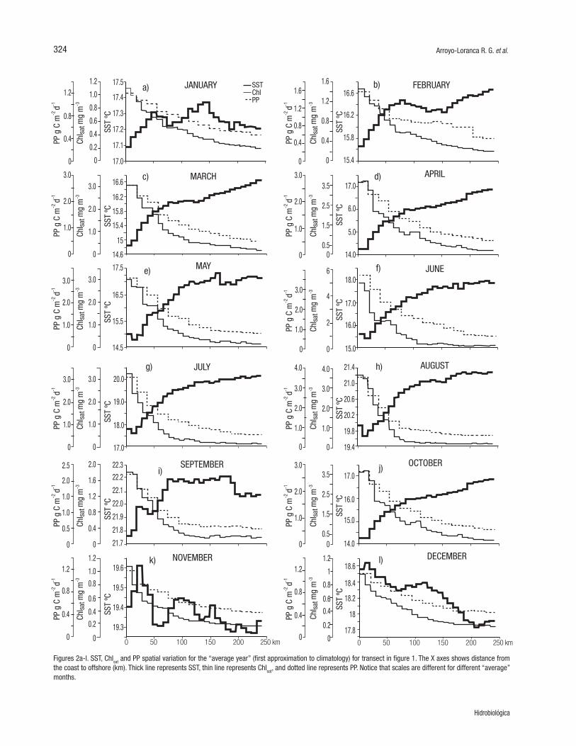
In general, the “average year” presents a very clear Chlsat and PP spa-tial variation from the coast to waters offshore, with higher values near the coast (up to ~120 km from shore), and lower values offshore (120 to 242 km) (Fig. 2). SST showed a different pattern of variation, with minima near the coast and maxima offshore from January through Oc-tober, and with a gradient reversal at the end of autumn and beginning of winter with maximum values near the coast. In the “average year,” when SST was lower near the coast than offshore, values inshore were from few tenths of one °C (in January and September) up to ~2.7 °C (in April and October) lower than offshore. During the “average No-vember,” SST varied one or two tenths of a degree around 19.4 °C,
Figure 1. Bahía Sebastián Vizcaíno and Punta Eugenia, Baja California Sur, México. The broken line (-----) is the sampled transect; the square ( ) is the geographic location for the generation of time series.
324 Arroyo-Loranca R. G. et al.
Hidrobiológica
Figures 2a-l. SST, Chlsat and PP spatial variation for the “average year” (first approximation to climatology) for transect in figure 1. The X axes shows distance from the coast to offshore (km). Thick line represents SST, thin line represents Chlsat, and dotted line represents PP. Notice that scales are different for different “average” months.
PP g
C m
-2 d
-1PP
g C
m-2
d-1
PP g
C m
-2 d
-1PP
g C
m-2
d-1
PP g
C m
-2 d
-1PP
g C
m-2
d-1
PP g
C m
-2 d
-1PP
g C
m-2
d-1
PP g
C m
-2 d
-1PP
g C
m-2
d-1
PP g
C m
-2 d
-1PP
g C
m-2
d-1
SST
ºCSS
T ºC
SST
ºCSS
T ºC
SST
ºCSS
T ºC
SST
ºCSS
T ºC
SST
ºCSS
T ºC
SST
ºCSS
T ºC
Chl sa
t mg
m-3
Chl sa
t mg
m-3
Chl sa
t mg
m-3
Chl sa
t mg
m-3
Chl sa
t mg
m-3
Chl sa
t mg
m-3
Chl sa
t mg
m-3
Chl sa
t mg
m-3
Chl sa
t mg
m-3
Chl sa
t mg
m-3
Chl sa
t mg
m-3
Chl sa
t mg
m-3
a) JANUARY
MARCH
MAY
JULY
SEPTEMBER
NOVEMBER
FEBRUARY
APRIL
JUNE
AUGUST
OCTOBER
DECEMBER
SSTChlPP
17.5
17.4
17.3
17.2
17.1
17.0
16.6
16.2
15.8
15.4
15
14.6
17.5
16.5
15.5
14.5
22.322.2
22.1
22.0
21.9
21.8
21.7
19.6
19.5
19.4
19.3
16.6
16.2
15.8
15.4
17.0
6.0
5.0
14.0
18.0
17.0
16.0
15.0
21.4
21.0
20.6
20.2
19.8
19.4
17.0
16.0
15.0
14.0
18.6
18.4
18.2
18
17.8
e)
i)
b)
f)
j)
c)
g)
k)
d)
h)
l)
1.2
0.8
0.4
0
3.0
2.0
1.0
0
1.2
1.0
0.8
0.6
0.4
0.2
0
3.0
2.0
1.0
0
2.0
1.6
1.2
0.8
0.4
0
1.2
1.00.8
0.6
0.40.2
0
1.6
1.2
0.8
0.4
0
3.5
2.5
1.5
0.50
6
4
2
0
4.0
3.0
2.0
1.0
0
3.5
2.5
1.5
0.50
1.2
1
0.8
0.60.4
0.2
0
1.6
1.2
0.8
0.4
0
3.0
2.0
1.0
0
4.0
3.0
2.0
1.0
0
3.0
2.0
1.0
0
3.0
2.0
1.0
0
3.0
2.0
1.0
0
3.0
2.0
1.0
0
3.0
2.0
1.0
0
2.5
2.0
1.0
1.0
0.5
0
0 50 100 150 200 250 km 0 50 100 150 200 250 km
1.2
0.8
0.4
0
1.2
0.8
0.4
0
3.0
2.0
1.0
0
20.0
19.0
18.0
17.0

325Phytoplankton in CCS off Punta Eugenia
Vol. 25 No. 3 • 2015
while in December it decreased from 18.6 °C near the coast to ~17.9 °C offshore (Fig. 2). In the “average year,” the spatial change of SST was monotonical from March through August, and in October. But often SST also presented a spatial distribution with values increasing and de-creasing successively. The spatial change of SST had two minima and two maxima in September and from December through February. The average November had several minima and maxima but, again, with a very small SST range (Fig. 2).
Inshore, the “average year” shows biological conditions separa-ted into two “seasons.” Chlsat was high inshore during March-August (“spring-summer”) (up to ~5 mg m-3 in June) and relatively low from September through February (“autumn-winter”) (1.0 - 1.8 mg m-3), with exception of October when Chlsat was up to >3.5 mg m-3. PP had a similar pattern of variation as that of Chlsat, with high values near the coast, up to ~3.5 g C m-2 d-1, in June, July and August, and relatively low values (~1.2 g C m-2 d-1) in November, December and January. Offshore, both Chlsat and PP had very small ranges, with minima of 0.2 mg m-3 and ~0.4 g C m-2 d-1 from October through January, and maxima of 0.4 mg m-3 and ~0.5 g C m-2 d-1 from February through September (Fig. 2).
The year after year variation of the SST transect had clear seasonal and interannual components. In what follows only some particular tran-sects will be illustrated as examples. Close to the coast, the SST ran-ge for the study period was 12.8 °C to 26.9 °C; and furthest-offshore (~240 km) the SST range was15.6 °C to 23.6 °C. Close to the coast, SST yearly minimum occurred in April of seven years (with the warmest April in 1998, 16.8 °C), in March of four years, and in May of four years. Close to the coast, SST yearly maximum occurred in September of ele-ven years (with the highest September maximum in 2012, 26.9 °C), and in August of four years (Fig. 5, Table 1).
Yearly minimum SST values for waters furthest-offshore were re-corded for February of eight years (with the warmest February in 1998,
18.0 °C), but four years had the minima in March, and in other cases minima were in spring or autumn months (April, May, and December). Yearly maximum SST values for waters furthest-offshore were recorded for September of twelve years (with the warmest September in 2012, 23.6 °C), but 1998 had the offshore maximum in January (19.1 °C), and 2000 and 2010 had the maxima in August (Table 1).
The timing of the SST gradient reversal to have maximum values near the coast and lower values offshore differed from year to year. In most cases this gradient was present during two months, sometimes starting in November and sometimes in January. But in two years the reversal of the gradient was not clear; and there were very particu-lar cases with this gradient present from August through November in 2008, and from September through December in 2005, 2009, and 2012.
In the year to year variation of the SST transect the presence of several minima and maxima did not present a clear temporal pattern of variation. Some examples are illustrated for March and November 1998, November 2000 (Fig. 3) (largest SST difference between suc-cessive minimum and maximum were between one and 1.8 oC), and November 2008 (largest SST difference between successive minimum and maximum was about 0.4 oC) (Fig. 4).
The year after year variation of the transect had a coastal zone with relatively high Chlsat and PP extending from the coast up to 150 km, often to only ~80 km. This inshore region had Chlsat and PP variations with clear seasonal and interannual components. Close to the coast, the Chlsat and PP ranges for the study period were 0.4 to 26.3 mg m-3, and 0.6 to 8.7 g C m-2 d-1, respectively, with the lowest values corres-ponding to1998 (Table 2). Sometimes, the Chlsat maximum was not near the coast but between 25 and 50 km from the coast (i.e., March 2000, Fig. 3, March 2008, and March 2009, Fig. 4). Inshore, the years 2008 and 2010-2012 had Chlsat and PP values exceptionally high (Table 2).
Table 1. Minimum and maximum SST (°C) values for inshore (IS) and furthest-offshore (FO) waters of the California Current System off Punta Eu-genia, for each year, and the month in which they occurred.
Years
“IS” 98 99 00 01 02 03 04 05 06 07 08 09 10 11 12
SST 16.8 13.5 14.6 15.2 14.5 13.6 15.1 14.2 13.6 13.9 13.4 13.6 13.9 13.4 14.1
Min Apr Mar Mar Apr Apr May May Apr Mar Apr Apr Apr May May Mar
SST 20.1 19.0 20.8 21.9 22.1 21.3 22.2 23.8 24.1 22.3 25.5 25.8 19.5 20.9 26.9
Max Sep Sep Sep Aug Aug Sep Sep Sep Aug Sep Sep Sep Aug Sep Sep
“FO” 98 99 00 01 02 03 04 05 06 07 08 09 10 11 12
SST 18.0 16.0 17.0 16.6 16.3 17.2 16.5 17.0 16.2 16.6 16.3 16.1 15.9 15.6 16.5
Min Feb Feb Feb Feb Feb Apr Feb Feb Mar May Mar Mar Dec Mar Feb
SST 19.1 20.0 22.1 22.3 22.6 21.8 22.3 22.5 23.1 22.2 21.9 23.1 19.8 21.3 23.6
Max Jan Sep Aug Sep Sep Sep Sep Sep Sep Sep Sep Sep Aug Sep Sep

326 Arroyo-Loranca R. G. et al.
Hidrobiológica
Fgures 3a-d. Comparison of the SST, Chlsat and PP spatial variation in transect shown in figure 1 for 1998 (El Niño year) and 2000 (La Niña year) in the California Current System. The X axes shows distance from the coast to offshore (km). Thick line represents SST from AVHRR (pixel size 4x4 km2), thin line represents Chlsat, and dotted line represents PP. Notice that scales are different for panel c.
Close to the coast, in the year-to-year variation, Chlsat and PP were lowest in December of five years; but other years had Chlsat and PP minima in January, September, October, and November. The ranges for the Chlsat and PP yearly minimum values of the coastal region were 0.4 to 1.4 mg m-3, and 0.6 to 1.6 g C m-2 d-1 (Table 2). Close to the coast, Chlsat and PP yearly maxima occurred between March and August, with the highest maximum Chlsat in May 2010 (26.3 mg m-3), and the highest PP maximum in August 2011 (8.7 g C m-2 d-1) (Table 2).
Yearly minimum Chlsat values for waters furthest-offshore fluctua-ted around 0.1 mg m-3, while PP minima fluctuated in the range 0.3-0.5 g C m-2 d-1. There seemed to be no particular trend for these low values to occur within a particular period of the year. In these waters, maximum Chlsat values fluctuated within the range 0.2-0.5 mg m-3, and maxima PP in the range 0.6-0.9 g C m-2 d-1, and they were recorded for months between January and July (Table 2).
In March of 1998 (El Niño year) SST was larger (up to 3 °C), and Chlsat and PP were lower, than in March 2000 (La Niña year) (Fig. 3a, c). In March of 1998 Chlsat was ~0.8 mg m-3 close to the coast and only for the first ~10 km, with values as low as 0.4 mg m-3 at 50 km, and even lower further offshore; PP was 1.1 g C m-2 d-1 close to the coast, decrea-sing to <0.9 g C m-2 d-1 beyond 50 km (Fig. 3a). In March of 2000 Chlsat was 1.0 - 2.2 mg m-3 from the coast to 50 km, decreasing abruptly to values <0.5 mg m-3 in waters further offshore; PP had values between 1.7 and 2.2 g C m-2 d-1 in the first 50 km from shore, and it also decrea-sed abruptly to <0.5 g C m-2 d-1 further offshore (Fig. 3c). In general, both Novembers (1998 and 2000) had relatively low and similar Chlsat (<0.6 mg m-3) and PP values (<0.9 g C m-2 d-1) (Fig. 3b, d). On the other hand, when comparing the transect data for 2008 (La Niña year) with those for 2009 (El Niño year) the values for the three variables were similar for the same month (Figs. 4a, c; and 4b, d).
The SST time series for the coastal location off Bahía Tortugas shows that there are clear seasonal and interannual variations (Fig. 5). It can be seen that the annual cycle dominates the SST variation. It is evident that maxima SST for 1998 and 1999 are lower than those for other years (20.1 and 19.0 °C, respectively), with the highest maximum for September 2012 (26.9 °C) (Table 1, Fig. 5). Lowest SST minima were those of 1999, 2008 and 2011 (~13.5 °C), and highest SST minimum was the one for 1998 (16.8 °C) (Table 1, Fig. 5).
The Chlsat and PP time series also show a clear dominating annual cycle, with an interannual component of variation (Figs. 6a, b). The Chl-
sat time series shows higher “spring-summer” values in 2008 and in 2010-2012 than in the other years, with the lowest values in 1998, and relatively low values in 2009 (Fig. 6a). “Spring-summer” Chlsat increa-sed from 1998 through 2000, then it had a general tendency to decrea-se from 2000 to 2005, to then change irregularly through 2012 (Fig. 6a). The PP time series also shows “spring-summer” values increasing from 1998 through 2000, then it had a general tendency to decrease from 2000 to 2005-2006, to then increase from 2007 through 2011, and finally decrease in 2012 (Fig. 6b). The highest “spring-summer” PP value was the one for August 2011 with 8.7 g C m-2 d-1, and the lowest maximum value was the one for June 1998 with 2.4 g C m-2 d-1 (Table 3, Fig. 6b).
Based on the Chlsat time series, the SST, Chlsat, and PP time series were separated into five-year periods and then the spectral analysis was obtained. In each case, figure 7 shows the spectra for the three periods. The spectral analysis of the three variables confirms that most of the variance was in the annual and interannual periods. The interan-nual variation is clearly appreciated when comparing the annual peaks (maxima) of the spectra for the three different periods (Fig. 7). In the cases for the PP and Chlsat spectra for the last five-year period, the increase of the seasonal variation is very clear with respect to those of the first two five-year periods. The variation of the SST spectra for the second and third periods is not significantly different, but both are higher than the one for the first period (Fig. 7).
a)
b)
b)
c)
c)
c)
d)
PP g
C m
-2 d
-1PP
g C
m-2
d-1
PP g
C m
-2 d
-1PP
g C
m-2
d-1
SST
ºCSS
T ºC
SST
ºCSS
T ºC
Chl sa
t mg
m-3
Chl sa
t mg
m-3
Chl sa
t mg
m-3
Chl sa
t mg
m-3
NOVEMBER 2000
MARCH 2000
NOVEMBER 1998
MARCH 1998
19
18
17
17
16
15
19
18
17
19
18
17
1.0
0.8
0.6
0.4
0.2
0
2.0
1.0
0
1.0
0.8
0.6
0.4
0.2
0
0 50 100 150 200 250 km
0 50 100 150 200 250 km
0 50 100 150 200 250 km
0 50 100 150 200 250 km
1.0
0.8
0.6
0.4
0.2
0
1.2
1.0
0.8
0.6
0.4
0.2
2.0
1.0
0
1.2
1.0
0.8
0.6
0.4
0.2
1.2
1.0
0.8
0.6
0.4
0.2

327Phytoplankton in CCS off Punta Eugenia
Vol. 25 No. 3 • 2015
The Chlsat distributions are not normal. Thus, non-parametric Mann-Whitney tests were used to compare “spring-summer” and “autumn-winter” data sets for pairs of years of the inshore (0-80 km) transect portion (at the 95% confidence level). The differences were only sig-nificant when comparing 1998 (El Niño year) data with those of 2000 (La Niña year) for both periods, “spring-summer” and “autumn-winter” (Table 3).
DISCUSSION
Durazo et al. (2005) reported a clear contribution of low salinity and low temperature subarctic water in the upper 100 m of the water co-lumn in the CCS off the Baja California peninsula, in the period October 2002 - April 2003. These latter authors did not detect a strong biologi-cal signal, beyond the seasonal cycle, caused by the presence of this colder and fresher water. El Niño 2002-2003 was marked by cold and fresh surface waters during 2002 and weak warming in early 2003 (Venrick et al., 2003). Possibly, El Niño and the intrusion of subarctic water nullified the effect of each other on the biological response of the pelagic environment of the CCS. Herrera-Cervantes et al. (2013) used principal components analysis to describe the interannual SST
Table 2. Minimum and maximum Chlsat (mg m-3) and PP (g C m-2 day-1) values for inshore (IS) and furthest-offshore (FO) waters of the California Current System off Punta Eugenia, for each year, and the month in which they occurred.
Years
“IS” 98 99 00 01 02 03 04 05 06 07 08 09 10 11 12
Chlsat 0.4 0.5 0.5 0.7 0.8 0.5 0.6 0.5 0.7 0.8 0.5 0.5 0.7 1.4 0.5
Min Sep Jan Nov Dec Jan Jan Dec Oct Nov Dec Oct Dec Jan Dec Oct
PP 0.6 0.9 0.8 1.1 1.3 0.8 0.9 0.9 1.1 1.2 0.9 0.9 1.0 1.6 0.9
Min Nov Jan Nov Dec Jan Jan Dec Oct Nov Dec Oct Dec Jan Dec Oct
Chlsat 1.9 4.8 8.6 4.6 5.6 4.1 3.3 2.6 8.2 4.1 20.9 6.9 26.3 18.3 17.4
Max Jun Apr Jul May Aug Jun Jun Apr May Jun Apr Apr May Jun Mar
PP 2.4 2.6 5.8 4.1 4.6 3.9 3.8 3.6 3.9 4.9 4.4 5.7 6.5 8.7 5.2
Max Jun Apr May May Aug May Jun Apr May Jun Apr Apr May Aug Mar
“FO” 98 99 00 01 02 03 04 05 06 07 08 09 10 11 12
Chlsat 0.1 0.1 0.1 0.1 0.1 0.1 0.1 0.1 0.1 0.1 0.1 0.1 0.1 0.1 0.1
Min Aug Oct Jul Dec May Mar Sep Dec Jun Jul Aug Aug Mar Aug Aug
PP 0.4 0.3 0.4 0.3 0.4 0.3 0.3 0.3 0.5 0.5 0.4 0.4 0.4 0.4 0.4
Min Aug Oct Mar Dec May Mar Nov Dec Jun Jul Aug Sep Dec Jul Aug
Chlsat 0.3 0.2 0.2 0.2 0.3 0.3 0.3 0.3 0.2 0.3 0.3 0.2 0.3 0.5 0.4
Max Jan Feb May Feb Feb May Mar May May Feb Apr Jun Jul Mar Apr
PP 0.8 0.6 0.6 0.6 0.9 0.9 0.6 0.9 0.9 0.9 0.9 0.6 0.8 0.8 0.8
Max Jan Apr May Jun Jul May Jun Jun May Feb Apr Jun Jul Mar Apr
Table 3. Results of the Mann-Whitney tests comparing Chlsat data sets from pairs of years, at the 95% confidence level.
“Spring- 1998 vs. 2000 n = 108, p <<0.0001Summer” 2008 vs. 2009 n = 108, p = 0.46
2000 vs. 2009 n = 108, p = 0.079
“Autumn- 1998 vs. 2000 n = 108, p = 0.0006Winter” 2008 vs. 2009 n = 108, p = 0.79
2000 vs. 2009 n = 108, p = 0.11
and Chlsat variability patterns in the area off Punta Eugenia, 26-29o N, 113-116o W. Herrera-Cervantes et al. (2013) concluded that the area is divided into coastal and deeper offshore waters, and suggested that ENSO cycles dominate the SST and Chlsat interannual variations in coas-tal waters, while in deep waters they were driven more by the intrusion of subarctic water than by ENSO cycles. However, not considering the 1997-1998 El Niño, our Chlsat and PP time series data from the coastal

328 Arroyo-Loranca R. G. et al.
Hidrobiológica
location (Fig. 6a, b), and those from the inshore-offshore transect (Table 2) do not show any significant effect of ENSO cycles and the intrusion of subarctic water in our study area. Statistical testing showed that only the 1997-1998 El Niño had a significant biological impact, with a re-duction of Chlsat and PP, and only in the inshore area (0-80 km from the coast). Time series for sea level and the MEI index show that in 2000 La Niña conditions were weak (Bograd et al., 2000) (Fig. 6).
There are two types of ENSO events: the Eastern-Pacific (EP) type that has maximum SST anomalies centered over the eastern tropical Pacific cold tongue region; and the Central-Pacific (CP) type that has the anomalies near the International Date Line (Kao & Yu, 2009). The CP El Niño is also referred to as the El Niño Modoki (similar to but not the same as El Niño) (Ashok et al., 2007). The propagating features of the SST anomalies from the equator to the northeastern Pacific is weaker and less clear in the CP type of ENSO than in the EP type. While the EP ENSO is known to be characterized by subsurface temperature anomalies propagating across the Pacific basin, the CP ENSO is found to be associated more with subsurface ocean temperature anomalies that develop in situ in the central Pacific (Ashok et al., 2007). Several methods have been proposed to identify the two types of ENSO, which include using SST or subsurface ocean temperature information. The 1997-1998 event was an EP type El Niño, but the XXI century events have been of the CP type (Lee & McPhaden, 2010), and this explains the non-significant effect of the XXI century El Niño events on the biology of our study area.
Satellite SST and Chlsat data are based on electromagnetic radiation data, and this makes them an approximation to reality. In the case of SST the approximation is much better because infrared radiation only has to be corrected to avoid cloud contamination, and for atmospheric absorption, primarily by water vapor. The MODIS infrared sensor (11 µm) is a heritage of the AVHRR sensor with improved precision. SST sensors show remarkable agreement (McClain et al., 1985; Armstrong et al., 2012). However, when comparing AVHRR with Aqua-MODIS SST data for the CCS, Armstrong et al. (2012) found that MODIS SST showed higher gradients than those derived from AVHRR.
In the case of Chlsat, algorithms applied to radiation data provide a very good approximation to in situ chlorophyll concentrations when values are low (case I waters with Chl ≤1.5 mg m-3), but comparisons between Chlsat and in situ Chl is not as good when values are high (case II waters with Chl ≥1.5 mg m-3) (Gordon et al., 1983). Caution should be exercised when dealing with case II waters Chlsat absolute values, paying more attention to tendencies for spatial and temporal changes. Nevertheless, Chlsat time series are very consistent; their seasonal cy-cles and the space variation behave very much as expected according to physical phenomena such as the movement of water masses and the occurrence of upwelling events (Santamaría-Del-Ángel et al., 1994). Ramirez-León et al. (2015) compared Gulf of California Chlsat from the sensors Coastal Zone Color Scanner (CZCS), SeaWIFS, and Aqua-MO-DIS, and found that they tend to agree well at low Chlsat values but differ at high values. The gulf Case II waters Chlsat from CZCS were as much as three times those from SeaWIFS and Aqua-MODIS. Chlsat from the latter two sensors agreed in most of the cases, but with Chlsat >2 mg m-3 sometimes those from Aqua-MODIS were larger than those from SeaWIFS, by as much as 30%. In our study, SeaWIFS and AVHRR data were used in addition to those from Aqua-MODIS to include the EP El Niño event of 1997-1998. Aqua-MODIS was put into orbit in 2002 and it is still operational. SeaWIFS produced data during 1997-2010.
Figures 4a-d. Comparison of the SST, Chlsat and PP spatial variation in transect shown in figure 1 for 2008 (La Niña year) and 2009 (El Niño year) in the Cali-fornia Current System.. The X axes shows distance from the coast to offshore (km). Thick line represents SST from Aqua-MODIS (pixel size 9x9 km2), thin line represents Chlsat, and dotted line represents PP. Notice that scales for SST are the same for all panels, but those for Chlsat and PP are the same only for panels a and c, and separately for panels b and d.
The Chlsat and PP seasonal cycle has a close relationship with the dynamics of the CCS. The flux of the California Current increases and coastal upwelling intensifies in April promoting a strong seasonal biolo-gical signal. The core of the equator-ward flux separates the biologically rich inshore region from the offshore region, at 100-200 km from the coast (Espinosa-Carreón et al., 2004; Durazo et al., 2010).
The study period started at the end of the last “warm” phase (end of 1997) and ended at the peak of the present “cold” phase of the PDO
a)
b)
c)
d)
PP g
C m
-2 d
-1PP
g C
m-2
d-1
PP g
C m
-2 d
-1PP
g C
m-2
d-1
SST
ºCSS
T ºC
SST
ºCSS
T ºC
Chl sa
t mg
m-3
Chl sa
t mg
m-3
Chl sa
t mg
m-3
Chl sa
t mg
m-3
NOVEMBER 2009
NOVEMBER 2008
MARCH 2009
MARCH 2008
22
20
18
16
14
22
20
18
16
14
22
20
18
16
14
22
20
18
16
14
12
0.8
0.4
0
12
0.8
0.4
0
0 50 100 150 200 250 km
0 50 100 150 200 250 km
0 50 100 150 200 250 km
0 50 100 150 200 250 km
1.41.21.00.80.60.4
0.20
1.41.21.00.80.60.4
0.20
4.0
3.0
2.0
1.0
0
4.0
3.0
2.0
1.0
0
7.5
6.0
4.0
2.0
0.0
7.5
6.0
4.0
2.0
0.0

329Phytoplankton in CCS off Punta Eugenia
Vol. 25 No. 3 • 2015
(Fig. 8). However, maximum SST values in the coastal location in gene-ral increased throughout most of our study period, from 1999 through 2009, to then change irregularly in 2010-2012; and minimum SST va-lues had no particular trend (Fig. 5). The irregular temporal variations of SST values at the coast, and the presence of several minima and maxima in the SST transect (such as those illustrated in figures 3 and 4), also without a clear temporal pattern of variation, may indicate a strong coastal influence of mesoscale phenomena such as eddies and meanders, like those reported by Durazo et al. (2005). These mesoscale phenomena affect the biological productivity of the area, as described by Henson and Thomas (2007a, b). Espinosa-Carreón et al. (2012) des-cribed the effect of mesoscale processes on surface and subsurface chlorophyll a distributions with data from three cruises carried on in January, April, and July 2000. These latter authors concluded that the biological response to mesoscale processes is very difficult to assess and interpret because of changes of the phytoplankton vertical distri-bution. Our results show that the hydrographic line parallel to the coast, chosen by Espinosa-Carreón et al. (2012) at 130 km from shore, is within the offshore region, where phytoplankton biomass is low and has a small variation. In order to define fluxes in the mesoscale pro-cesses, Espinosa-Carreón et al. (2012) applied the geostrophic method with salinity and temperature data from 0 to 500 m depth, which did not allow them to describe the inshore zone. Thus, strictly speaking it is not possible to compare their results with ours.
In the inshore region, the winter surface Countercurrent (Lynn & Simpson, 1987) should clearly produce higher SST, and lower Chlsat and PP values than those for summer. The Coriolis effect should cause the surface Countercurrent to inhibit upwelling in winter, because it tends to pile up the water near the coast. However, Chlsat and PP data often showed that winter values were relatively high, indicating that possi-bly the surface Countercurrent is not present, or there are mesoscale phenomena, such as eddies and meanders, affecting the fluxes in the coastal region as suggested with hypothetical examples in fig. 9. The SST spatial distribution, with minima and maxima, often suggests the presence of these mesoscale phenomena (i.e., Fig. 3), similar to those
described by Durazo et al. (2010). During winter, if the eddies and/or meanders were anti-cyclonic and adjacent to the coast, they could have nullified the Countercurrent and even produce a local southward and offshore flux (Fig. 9), with coastal upwelling and relatively high Chlsat and PP values (up to >1.2 mg m-3, and >3 g C m-2 d-1). As a comparison, in the Gulf of California, during the non-upwelling season Chlsat collap-ses down to <0.1 mg m-3 (Santamaría-del-Ángel et al., 1999).
The PP graphs parallel those of Chlsat. Chlsat dominated the varia-bility in PP, even though the calculated PP fields depend also on SST, photosynthetically available radiation, and day length, as was also re-ported by Álvarez-Molina et al. (2013) for the Gulf of California. PP data had less variability than those for Chlsat because PP is integrated for the whole euphotic zone while Chlsat is only for the first optical depth. When Chlsat is low the euphotic zone is deeper and integration with depth increases PP.
Possibly, our highest PP values for inshore waters, and for “spring-summer,” are overestimations because the VGPM model assumes a well-mixed euphotic zone with a homogeneous vertical distribution of chlorophyll. In nutrient rich coastal areas the chlorophyll maximum is at the surface with values decreasing with depth, and assuming no vertical chlorophyll change produces overestimations of PP. PP values higher than 4 g C m-2 d-1 (i.e., maxima for the last five years in figure 6) are unrealis-tic and should be taken with caution, considering only the temporal and spatial trends with no regard to absolute values. Álvarez-Molina et al. (2013) used the Oregon State University PP web page to report PP values for the central Gulf of California and expressed that it is possible that the highest VGPM values for the nutrient rich Guaymas basin upwelled waters (up to 7.8 g C m-2 d-1) were overestimated by >50%. These latter authors expressed that nevertheless the trend of their PP data variation was co-rrect with high values during the upwelling season and very low values during summer. The trends of our PP data variation are also correct, with higher values during the “spring-summer” upwelling period than during “autumn-winter”; and the annual cycles and interannual variations des-cribed for the transect, and in the time series for the coastal location off Bahía Tortugas, should also be correct.
Figure 5. SST time series for the coastal location immediately off Bahía Tortugas, Baja California Sur, México.
SST
Years
Tem
pera
ture
(ºC)

330 Arroyo-Loranca R. G. et al.
Hidrobiológica
Figures 6a-d. Time series of Chlsat, and PP for the coastal location off Bahía Tortugas; the MEI (Multivariate El Niño Index), and the NPDO (North Pacific Decadal Os-cillation) index, for the study period (1998-2012).
mg•
m-3
Stan
dard
dev
iatio
nsSt
anda
rd d
evia
tions
g C
m-2
d-1
a)
b)
c)
d)
Years
Years
Years
Years
PP
MEI
NPDO
Chlsat

331Phytoplankton in CCS off Punta Eugenia
Vol. 25 No. 3 • 2015
PP data obtained directly by water sampling and 14C incubations are very scarce, and it is difficult to do a comparison with satellite de-rived data. Strictly, the comparison between the VGPM data and 14C estimates is not appropriate because the two sets of data have tota-lly different time and space scales: the VGPM data are averages for 18×18 km2 (324 km2) areas and for one month, whereas the 14C data are instantaneous point measurements. Gaxiola-Castro et al. (2010) reported 14C PP data for the CCS off the Baja California peninsula, for
four cruises every year in the 1998-2007 period. The majority of their sampling locations were >50 km from shore. They averaged their data set to generate a mean distribution for their study area and reported PP values in mg C m-2 h-1. Transforming their average values to g C m-2 d-1, their offshore values are 0.4-0.6 g C m-2 d-1, which are in very good agreement with our PP values. Their average values for the inshore region fluctuate between 1.0 and 1.5 g C m-2 d-1, which again are in relatively good agreement with our values considering that most of their
Figures 7a-c. Variance spectra of the five-year periods time series for the coastal location off Bahía Tortugas. a)SST. b) Chlsat. c) PP. Broken line represents the first five-year period (1998-2002), dotted line represents the second (2003-2007), and the continuous line represents the third period (2008-2012).
a) b) c)
Func
tion
of v
aria
nce
Func
tion
of v
aria
nce
Func
tion
of v
aria
nce
Frequency (cicles year-1)
PPSST Chlsat
Figure 8. Smooth hypothetic curve of the NPDO (North Pacific Decadal Oscillation) index drawn over the graph from www.ncdc.noaa.gov/teleconnections/pdo/. The arrow indicates the study period (end of 1997 - October 2012).
3.0
2.0
1.0
0.0
-0.0
-2.0
-3.0
-4.01960 1970 1980 1990 2000 2010
NPDO
Stan
dard
dev
iatio
ns
Years

332 Arroyo-Loranca R. G. et al.
Hidrobiológica
Figures 9a-d. General spring-summer (a) and autumn-winter circulation, with the coastal surface countercurrent (b); hypothetical effects of meanders (c), and eddies (d) on autumn-winter coastal circulation and upwelling.
sampling sites were not close to shore. Sosa-Ávalos et al. (2010) repor-ted a detailed spatial distribution of PP for the CCS off Baja California, and for the four seasons. Sosa-Ávalos et al. (2010) used Chlsat and a model to estimate PP, and their maximum PP value for the coastal zone and for spring was 4.5 g C m-2 d-1, compared with our maximum value of 8.4 g C m-2 d-1. This indicates that PP data published in Oregon State University’s web site may overestimate the high values by as much as >80%. An adjustment of the photosynthetic parameters in the OSU PP VGPM algorithm is necessary for our geographic region, and that is an opportunity for future research.
ACKNOWLEDGEMENTS
We thank the Ocean Color NASA Program for allowing us the free use of its satellite imagery and the software to process them. We also thank NOAA´s Earth System Research Laboratory for providing the MEI data. The first author was granted a graduate studies fellowship by CONA-CyT. F. J. Ponce and J. M. Domínguez helped with the graphical design. J. Cepeda-Morales helped with the AVHRR SST data. The constructive criticisms of three anonymous reviewers helped to significantly improve our contribution.
a) b)
c) d)

333Phytoplankton in CCS off Punta Eugenia
Vol. 25 No. 3 • 2015
REFERENCES
Ahlstrom, E. h. 1965. Kinds and abundances of fishes in the California Current region based on egg and larval surveys. California Coope-rative Oceanic Fisheries Investigations Reports 10: 31-52.
ÁlvArEz-molinA, l. l., s. ÁlvArEz-BorrEgo, J. r. lArA-lArA & s. g. mArinonE. 2013. Annual and semiannual variations of phytoplankton biomass and production in the central Gulf of California estimated from sa-tellite data. Ciencias Marinas 39: 217-230.
Armstrong, E. m., g. WAgnEr, J. vAzquEz-CuErvo, t. m. Chin. 2012. Compari-sons of regional satellite sea surface temperature gradients derived from MODIS and AVHRR sensors. International Journal of Remote Sensing 33: 6639-6651.
Ashok, k., s. k. BEhErA, s. A. rAo, h. WEng & t. YAmAgAtA. 2007. El Niño Modoki and its possible teleconnection. Journal of Geophysical Re-search 112: C11007.
BAkun, A. & C. s. nElson. 1977. Climatology of upwelling related pro-cesses off Baja California. California Cooperative Oceanic Fisheries Investigations Reports 19: 107-127.
BAroCio-lEón, o. A., r. millÁn-núñEz, E. sAntAmAríA-dEl-ÁngEl, & A. gonzÁlEz-silvErA. 2007. Phytoplankton primary productivity in the euphotic zone of the California Current System estimated from CZCS ima-gery. Ciencias Marinas 33: 59-72.
BEhrEnfEld, m. J. & P. g. fAlkoWski. 1997. Photosynthetic rates derived from satellite-based chlorophyll concentration. Limnology & Ocea-nography 42: 1-20.
BogrAd, s. J., P. m. digiAComo, r. durAzo, t. l. hAYWArd, k. d. hYrEnBACh, r. J. lYnn, A. W. mAntYlA, f. B. sChWing, W. J. sYdEmAn, t. BAumgArtnEr, B. lAvAniEgos & C. s. moorE. 2000. The State of the California Current, 1999-2000: Forward to a New Regime? California Cooperative Oceanic Fisheries Investigations Reports 41: 26-52.
durAzo, r., g. gAxiolA-CAstro, B. lAvAniEgos, r. CAstro-vAldEz, J. gómEz-vAldés & A. d. s. mAsCArEnhAs Jr. 2005. Oceanographic conditions west of the Baja California coast, 2002-2003: A weak El Niño and subarctic water enhancement. Ciencias Marinas 31: 537-552.
durAzo, r., A. m. rAmírEz-mAnguilAr, l. E. mirAndA & l. A. soto-mArdonEs. 2010. Climatología de variables hidrográficas. In: Durazo, R. & G. Gaxiola-Castro (Eds.) Dinámica del Ecosistema Pelágico frente a Baja California 1997-2007. SEMARNAT, INE, CICESE & UABC. Méxi-co, D. F. pp. 25-57.
EsPinosA-CArrEón, t. l., P. t. struB, E. BEiEr, f. oCAmPo-torrEs & g. gAxiolA-CAstro. 2004. Seasonal and interannual variability of satellite deri-ved chlorophyll pigment, surface height, and temperature off Baja California. Journal of Geophysical Research 109: C03039.
EsPinosA-CArrEón, t. l., g. gAxiolA-CAstro, E. BEiEr, P. t. struB & J. A. kurCzYn. 2012. Effects of mesoscale processes on phytoplankton chlorophyll off Baja California. Journal of Geophysical Research 117: C04005.
fArgion, g. s., J. A. mCgoWAn & r. h. stEWArt. 1993. Seasonality of chloro-phyll concentrations in the California Current: A comparison of two methods. California Cooperative Oceanic Fisheries Investigations Reports 34: 35-50.
gAllAudEt, t. C. & J. J. simPson. 1994. An empirical orthogonal function analysis of remotely sensed sea surface temperature variability and its relation to interior oceanic processes off Baja California. Remote Sensing of Environment 47: 375-389.
gAxiolA-CAstro, g., J. CEPEdA-morAlEs, s. nÁJErA-mArtínEz, t. l. EsPinosA-CA-rrEón, m. E. dE-lA-Cruz-orozCo, r. sosA-ÁvAlos, E. AguirrE-hErnÁndEz & J. P. CAntú-ontivEros. 2010. Biomasa y producción del fitoplancton. In: Durazo, R. & G. Gaxiola-Castro (Eds.) Dinámica del Ecosistema Pelágico frente a Baja California 1997-2007. SEMARNAT, INE, CICE-SE & UABC. México, D. F. pp. 59-85.
gAY, P. s. & t. k. ChErEskin. 2009. Mean structure and seasonal variabili-ty of the poleward undercurrent off Southern California. Journal of Geophysical Research 114: C02007.
gordon, h. r., d. k. ClArk, J. W. BroWn, o. B. BroWn, r. h. EvAns, W. W. BroEnkoW. 1983. Phytoplankton pigment concentrations in the Middle Atlantic Bight: Comparison of ship determinations and CZCS estimates. Applied Optics 22: 20-35.
hEnson, s. A. & A. C. thomAs. 2007a. Phytoplankton scales of variability in the California Current System: 2. Latitudinal variability. Journal of Geophysical Research 112: C07018.
hEnson, s. A. & A. C. thomAs. 2007b. Interannual variability in timing of bloom initiation in the California Current System. Journal of Geophysical Research 112: C08007.
hErnÁndEz-CArmonA, g. 1988. Evaluación, crecimiento y regeneración de mantos de Macrocystis pyrifera en la costa occidental de la pe-nínsula de Baja California, México. Tesis de Maestría en Ciencias. IPN-Centro Interdisciplinario de Ciencias Marinas, La Paz. 157 p.
hErrErA-CErvAntEs, h., s. E. lluCh-CotA, d. B. lluCh-CotA & g. gutiérrEz-dE-vElAsCo. 2013. Interannual correlations between sea surface temperature and concentration of chlorophyll pigment off Punta Eugenia, Baja California, during different remote forcing conditions. Ocean Science Discussions 10: 853-882.
huYEr, A. 1983. Coastal Upwelling in the California Current System. Pro-gress in Oceanography 12: 259-284.
kAo, h. Y. & J. Y. Yu. 2009. Contrasting Eastern-Pacific and Central-Paci-fic Types of ENSO. Journal of Climate 22: 615-632.
kirk J. t. o. 1994. Light and photosynthesis in aquatic ecosystems. Cambridge University Press, New York. 509 p.
lAdAh, l., J. A. zErtuChE-gonzÁlEz & g. hErnÁndEz-CArmonA. 1999. Giant kelp (Macrocystis pyrifera, Phaeophyceae) recruitment near its southern limit in Baja California after mass disappearance during ENSO 1997-1998. Journal of Phycology 35: 1106-1112.
lEE, t. & m. J. mCPhAdEn. 2010. Increasing intensity of El Niño in the cen-tral-equatorial Pacific. Geophysical Research Letters 37: L14603.
lEón g. & m. muCiño. 1996. Pesquería de abulón. In: M. Casas & G. Ponce (Eds.). Estudio del potencial pesquero y acuícola de Baja California Sur. SEMARNAP, Gobierno del Estado de Baja California Sur, FAO, UABCS, CIBNOR, CICIMAR-IPN & CET del Mar, La Paz, México. pp. 15-41.

334 Arroyo-Loranca R. G. et al.
Hidrobiológica
lluCh-BEldA, d. 2000. Centros de Actividad Biológica en la costa oc-cidental de Baja California. In: Lluch-Belda, D., J. Elourduy-Garay, S. E. Lluch-Cota & G. Ponce-Díaz (Eds.) BAC: Centros de Actividad Biológica del Pacífico Mexicano. CIBNOR, CICIMAR-IPN, CONACYT. México, D. F. pp. 49-64.
lYnn, r. J. & J. J. simPson. 1987. The California current system: The sea-sonal variability of its physical characteristics. Journal of Geophysi-cal Research 92 (C12): 12,947-12,966.
mCClAin, E. P., W. g. PiChEl, C. C. WAlton. 1985. Comparative performance of AVHRR-based multichannel sea surface temperature. Journal of Geophysical Research 90: 11587-11601.
mAnn k. h. & J. r. n. lAziEr. 2006. Dynamics of Marine Ecosystems: Biological-Physical Interactions in the Oceans. Third Edition. Blac-kwell Publishing, Oxford. 440 p.
nEWmAn, m., J. P. ComPosE & m. A. AlExAndEr. 2003. ENSO-Forced Variabili-ty on the Pacific Decadal Oscillation. Journal of Climate 16: 3,856-3,857.
NOAA (National Oceanic and Atmospheric Administration). 2013a. Phy-sical Sciences Division of the Earth System Research Laboratory. Available on line: http://www.esrl.noaa.gov/psd/enso/mei/ (web site visited in January 2013).
NOAA (National Oceanic and Atmospheric Administration). 2013b. Phy-sical Sciences Division of the Earth System Research Laboratory. Available on line: http://www.ncdc.noaa.gov/teleconnections/pdo/ (web site visited in January 2013).
OCEAN COLOR. 2012. Available on line: http://oceancolor.gsfc.nasa.gov/ (web site visited in October-November 2012).
OSU (Oregon State University) PP site. 2012. Available on line: http://www.science.oregonstate.edu/ocean.productivity/index.php (web site visited in October-November 2012).
PElÁEz, J. & J. A. mCgoWAn. 1986. Phytoplankton pigment patterns in the California Current as determined by satellite. Limnology & Oceano-graphy 31: 212-225.
Putt, m. & B. B. PrézElin. 1985. Observations of diel patterns of photos-ynthesis in cyanobacteria and nannoplankton in the Santa Barbara
Channel during "El Niño". Journal of Plankton Research 7: 779-790.
rAmírEz-lEón, m. r., s. ÁlvArEz-BorrEgo, C. turrEnt-thomPson, g. gAxiolA-CAstro & g. hECkEl-dziEndziElEWski. 2015. Nutrient input from the Co-lorado River water to the northern Gulf of California is not required to maintain its pelagic ecosystem productive. Ciencias Marinas 41: 169-188.
rEid, J. l. 1988. Physical Oceanography. California Cooperative Oceanic Fisheries Investigations Reports 29: 42-65.
sAntAmAríA-dEl-ÁngEl, E., s. ÁlvArEz-BorrEgo, f. E. müllEr-kArgEr. 1994. Gulf of California biogeographic regions based on coastal zone color scanner imagery. Journal of Geophysical Research 99: 7411-7421.
sAntAmAríA-dEl-ÁngEl, E., s. ÁlvArEz-BorrEgo, r. millÁn-nuñEz & f. E. mü-llEr-kArgEr. 1999. Sobre el efecto de las surgencias de verano en la biomasa fitoplanctónica del Golfo de California. Revista de la Socie-dad Mexicana de Historia Natural 49: 207-212.
sChWArtzlosE r. A. & J. l. rEid. 1972. Near-Shore Circulation in the Cali-fornia Current. California Cooperative Oceanic Fisheries Investiga-tions Reports 16: 57-65.
sosA-ÁvAlos, r., g. gAxiolA-CAstro, B. g. mitChEll & J. CEPEdA-morAlEs. 2010. Parámetros fotosintéticos y producción primaria estimada a partir de sensores remotos durante 1999. In: Durazo, R. & G. Gaxio-la-Castro (Eds.) Dinámica del Ecosistema Pelágico frente a Baja California 1997-2007. SEMARNAT, INE, CICESE & UABC. México, D. F. pp. 319-331.
vEnriCk, E., s. BogrAd, d. ChECklEY, s. Cummings, r. durAzo, g. gAxiolA-CAstro, J. huntEr, A. huYEr, k. d. hYrEnBACh, B. E. lAvAniEgos, A. mAntYlA, f. B. sChWing, r. l. smith, W. J. sYdEmAn & P. A. WhEElEr. 2003. The state of the California Current, 2002-2003: Tropical and subarctic influen-ces vie for dominance. California Cooperative Oceanic Fisheries Investigations Reports 44: 28-60.
Recibido: 21 de noviembre de 2014.
Aceptado: 03 de junio de 2015.