QUASI-LIE ALGEBRAS

AND

QUASI-DEFORMATIONS

ALGEBRAIC STRUCTURES ASSOCIATED WITH TWISTEDDERIVATIONS

DANIEL LARSSON

Faculty of EngineeringCentre for Mathematical Sciences

Mathematics

MathematicsCentre for Mathematical SciencesLund UniversityBox 118SE-221 00 LundSweden

http://www.maths.lth.se/

Doctoral Theses in Mathematical Sciences 2006:1ISSN 1404-0034

ISBN 91-628-6739-3LUTFMA-1020-2006

c© Daniel Larsson, 2006

Printed in Sweden by KFS, Lund 2006

Organization Document name Centre for Mathematical Sciences Lund Institute of Technology

DOCTORATE THESIS IN MATHEMATICAL SCIENCES

Mathematics Date of issue

Box 118 February 2006 SE-221 00 LUND Document Number

LUTFMA-1020-2006 Author(s) Supervisors Daniel Larsson Sergei Silvestrov, Gunnar Sparr Sponsering organisation

Lund University, Marie Curie/Liegrits network, University of Antwerp, STINT, Crafoord Foundation

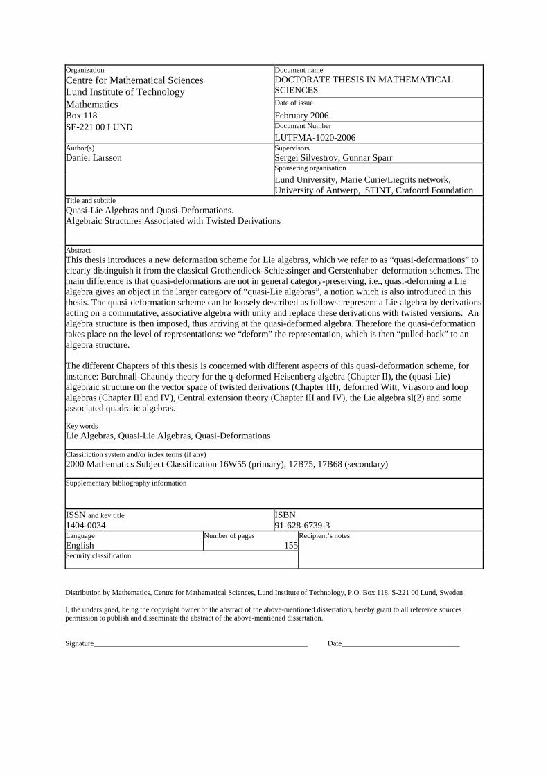
Title and subtitle Quasi-Lie Algebras and Quasi-Deformations. Algebraic Structures Associated with Twisted Derivations Abstract This thesis introduces a new deformation scheme for Lie algebras, which we refer to as “quasi-deformations” to clearly distinguish it from the classical Grothendieck-Schlessinger and Gerstenhaber deformation schemes. The main difference is that quasi-deformations are not in general category-preserving, i.e., quasi-deforming a Lie algebra gives an object in the larger category of “quasi-Lie algebras”, a notion which is also introduced in this thesis. The quasi-deformation scheme can be loosely described as follows: represent a Lie algebra by derivations acting on a commutative, associative algebra with unity and replace these derivations with twisted versions. An algebra structure is then imposed, thus arriving at the quasi-deformed algebra. Therefore the quasi-deformation takes place on the level of representations: we “deform” the representation, which is then “pulled-back” to an algebra structure. The different Chapters of this thesis is concerned with different aspects of this quasi-deformation scheme, for instance: Burchnall-Chaundy theory for the q-deformed Heisenberg algebra (Chapter II), the (quasi-Lie) algebraic structure on the vector space of twisted derivations (Chapter III), deformed Witt, Virasoro and loop algebras (Chapter III and IV), Central extension theory (Chapter III and IV), the Lie algebra sl(2) and some associated quadratic algebras. Key words Lie Algebras, Quasi-Lie Algebras, Quasi-Deformations Classifiction system and/or index terms (if any) 2000 Mathematics Subject Classification 16W55 (primary), 17B75, 17B68 (secondary) Supplementary bibliography information ISSN and key title ISBN 1404-0034 91-628-6739-3 Language Number of pages Recipient’s notes English 155 Security classification Distribution by Mathematics, Centre for Mathematical Sciences, Lund Institute of Technology, P.O. Box 118, S-221 00 Lund, Sweden I, the undersigned, being the copyright owner of the abstract of the above-mentioned dissertation, hereby grant to all reference sources permission to publish and disseminate the abstract of the above-mentioned dissertation. Signature__________________________________________________________ Date________________________________

Freedom is the freedom to say two plus two make four.If this is granted, all else follows.

Winston SmithNineteeneightyfour

(George Orwell)

Post hoc – ergo propter hoc.

iv

Acknowledgments

The set Important of important people surrounding any given person can be decom-posed into two, possibly empty (in which case we call it a sad life) subsets: Professionaland Friends of hopefully finite or countable cardinality.

In the present author’s case Important is comprised of:

Professional: Sergei Silvestrov, Jonas Hartwig, Fred Van Oystaeyen, Arnfinn Laudal,Gunnar Sparr, Victor Ufnarovski, Clas Löfwall, Gunnar Sigurdsson, Lars Hellström,Magnus Fontes, Anki Ottosson and Jaak Peetre.

Friends: Max, Lotta, Mum, Dad, Grandma, Grandpa, Mattias, Andreas, Robban, Mal-ice, Nina, Miško, Goro and Lena.

Details:∫Sergei: Obviously this thesis would not have been written without the guidance,lively, animated and heated discussions and cooperation with my supervisor Do-cent Sergei Silvestrov whose eager attitude toward me and mathematics saved manya day. We managed to find common ground in the area of algebra with my incli-nation toward the intersection between algebra and geometry and his toward oper-ator/representation theory and there found a little gold mine to explore. There isstill a lot of work ahead, Sergei!∫Gunnar: I am grateful to assistant supervisor Professor Gunnar Sparr for adviceand support of this work.∫Fred : A very big thanks goes out to Professor Fred Van Oystaeyen for sharingsome of his uncanny knowledge of all areas of algebra and in particular graded ringtheory and non-commutative geometry.∫Arnfinn, Victor and Clas: Thank you, Professor Arnfinn Laudal, Docent VictorUfnarovski and Professor Clas Löfwall for answers (to sometimes stupid questions,I admit), inspiration, friendship, suggestions and knowledge.∫Jonas, Gunnar and Lars: Fellow students of Sergei: Jonas Hartwig, Gunnar Sig-urdsson and Dr. Lars Hellström. In one way or another we suffered the same andgained the same. Thanks for all discussions and help on various things that onlyyou (and possibly me) know.∫Jaak: Thank you, Professor Jaak Peetre for your advice, encouraging words andbelief in me from, when was it, 1993 (?) to present.

1

∫Magnus: Thank you, Docent Magnus Fontes for support of this work.∫Anki: For help with all kinds of practical details, small or big, and also for alwaysgreeting me with a happy face, I thank Anki Ottosson.

We all have to eat and be clothed, so I gratefully acknowledge:

• The Liegrits Marie Curie network, Mittag-Leffler Institute (Stockholm, Sweden),Swedish Foundation for International Cooperation in Research and Higher Edu-cation (STINT), the Crafoord Foundation and the Non-commutative Geometry(NOG) program (ESF, European Science Foundation) for financial support.

• The Algebra and Geometry group, Department of Mathematics @ the Universityof Antwerp, Belgium, for support and excellent research environment.

And nally:

♥ Friends: You all know what you’ve done keeping me sane when balancing on theedge. A mere ’thank you’ could never be enough, but what more can I offer?Thank you all so much.

2

Contents

1 Introduction 7

2 Burchnall–Chaundy theory of q-Difference operators and q-deformed Heisen-berg algebras 312.1 Introduction . . . . . . . . . . . . . . . . . . . . . . . . . . . . . . . 312.2 A Burchnall–Chaundy type theorem . . . . . . . . . . . . . . . . . . . 34

3 Deformations of Lie Algebras using σ-Derivations 453.1 Introduction . . . . . . . . . . . . . . . . . . . . . . . . . . . . . . . 453.2 Some general considerations . . . . . . . . . . . . . . . . . . . . . . . 48

3.2.1 Generalized derivations on commutative algebras and UFD’s . . 483.2.2 A bracket on σ-derivations . . . . . . . . . . . . . . . . . . . 523.2.3 hom-Lie algebras . . . . . . . . . . . . . . . . . . . . . . . . 603.2.4 Extensions of hom-Lie algebras . . . . . . . . . . . . . . . . . 63

3.3 Examples . . . . . . . . . . . . . . . . . . . . . . . . . . . . . . . . . 683.3.1 A q-deformed Witt algebra . . . . . . . . . . . . . . . . . . . 683.3.2 Non-linearly deformed Witt algebras . . . . . . . . . . . . . . 713.3.3 An example with a shifted difference . . . . . . . . . . . . . . 80

3.4 A bracket on σ-differential operators . . . . . . . . . . . . . . . . . . . 823.5 A deformation of the Virasoro algebra . . . . . . . . . . . . . . . . . . 85

3.5.1 Uniqueness of the extension . . . . . . . . . . . . . . . . . . . 853.5.2 Existence of a non-trivial extension . . . . . . . . . . . . . . . 89

4 Quasi-hom-Lie Algebras, Central Extensions and 2-Cocycle-Like Identities 974.1 Introduction . . . . . . . . . . . . . . . . . . . . . . . . . . . . . . . 974.2 Definitions and notations . . . . . . . . . . . . . . . . . . . . . . . . 1004.3 Examples . . . . . . . . . . . . . . . . . . . . . . . . . . . . . . . . . 1034.4 Extensions . . . . . . . . . . . . . . . . . . . . . . . . . . . . . . . . 107

4.4.1 Equivalence between extensions . . . . . . . . . . . . . . . . . 1134.4.2 Existence of extensions . . . . . . . . . . . . . . . . . . . . . 1164.4.3 Central extensions of the (α, β, ω)-deformed loop algebra . . . 119

3

CONTENTS

5 Quasi-deformations of sl2(F) using twisted derivations 1275.1 Introduction . . . . . . . . . . . . . . . . . . . . . . . . . . . . . . . 1275.2 Qhl-algebras associated with σ-derivations . . . . . . . . . . . . . . . . 1295.3 Quasi-Deformations . . . . . . . . . . . . . . . . . . . . . . . . . . . 130

5.3.1 Quasi-Deformations with base algebra A = F[t] . . . . . . . . 1325.3.2 Deformations with base algebra F[t]/(t3) . . . . . . . . . . . . 139

4

CONTENTS

Preface

The present thesis covers five different papers (A, B, C, D and E) which more or lesscorrespond to the four non-introductory Chapters of the thesis. The sole exception isPaper D which is molded into Chapters 3 and 4. The papers are:

A. Larsson, D., Silvestrov, S.D., Burchnall-Chaundy Theory for q-Difference Operatorsand q-Deformed Heisenberg Algebras, J. Nonlinear Math. Phys. 10, Supplement 2(2003), 95–106.

B. Hartwig, J.T., Larsson, D., Silvestrov, S.D., Deformations of Lie algebras using σ-derivations, Journal of Algebra 295 (2006), 314–361.

C. Larsson, D., Silvestrov S.D., Quasi-hom-Lie algebras, central extensions and 2-cocycle-like identities, Journal of Algebra 288 (2005), 321–344.

D. Larsson, D., Silvestrov, S.D., Quasi-Lie algebras, Preprints in Mathematical Sci-ences 2004:30, LUTFMA-5049-2004, to appear in Cont. Math. 391 Amer.Math. Soc. 2005.

E. Larsson, D., Silvestrov, S.D., Quasi-deformations of sl2(F) using twisted derivations,Preprints in Mathematical Sciences 2004:26, LUTFMA-5047-2004, Submitted torefereed journal.

In addition, there is a review-like paper:

F. Larsson, D., Silvestrov, S.D., The Lie algebra sl2(F) and quasi-deformations, Czechoslo-vak Journal of Physics 55 (2005) 11, 1467–1472.

5

CONTENTS

6

Chapter 1

IntroductionTo a very large extent mathematics is a (maybe actually the?) science of symmetries. Thesesymmetries appear both in “nature” and within mathematics itself. Fundamental to bothmathematics and, for instance, to the quantum field theories, is the notion of a Lie group1.In the case of physical theories, a Lie group is often an object governing the inherent sym-metries of the theory and thus, in its extension, provided the theory is correct, nature. Forinstance rotational symmetries in ordinary three-dimensional Euclidean space constitutesa Lie group known as real SO(3). This is the set of 3×3-matricesA satisfyingA−1 = At

and det(A) = 1.However, these symmetry groups are often very complicated globally. Therefore one

needs a local version and a way to go from the local to the global2. This is provided bythe Lie algebra and the “exponential map”,

exp :

LOCAL

Lie Algebra, g

−→

GLOBAL

Lie Group, G

.

To each Lie group is associated a specific Lie algebra. However, there can be severalLie groups with the same Lie algebra, so this is not a one-to-one correspondence. Thelocal nature of a Lie algebra makes it convenient to consider as a space of “infinitely smallsymmetries”. For example, the Lie algebra to SO(3) is so(3), the space of skew-symmetric3× 3-matrices, which therefore can be viewed as “infinitesimal rotational symmetries”.

A very important added feature which is crucial in physics is that Lie groups and Liealgebras act on certain vector spaces. In the case of SO(3), elements of this group ro-tate vectors in three-dimensional Euclidean space. But this is only one possible way toview this group, one particular “representation”. There are others. A fundamental, andin general very difficult, problem is to determine all (at least finite-dimensional) repre-sentations of a given group, i.e., all possible guises it can take. For SO(3) this is actuallywell-known, at least when considering continuous complex linear representations. Thesame discussion applies to Lie algebras with the slight bonus that it is in general a simpler(not to say simple!) task finding representations of a Lie algebra than the correspondingLie group. Once representations of the Lie algebra are known it is sometimes possible todetermine the representations of the underlying Lie group.

It is therefore quite natural to infer that to fully comprehend the symmetries of natureit is extremely important to have a thorough understanding of Lie groups and Lie algebras,

1These objects were first studied by the Norwegian mathematician Sophus Lie (1842–1899) in connectionwith symmetries of solutions to differential equations, hence the name.

2Although, for some physical problems the global version is not given within the problem and so "nature"then only supplies the local symmetries.

7

CHAPTER 1.

i.e., the objects representing global and local symmetries. In fact, the category of Liealgebras is one of the two central notions underlying and lurking behind all conceptsappearing in this thesis. The other is the notion of a derivation.

As should be well-known to everybody a derivation on an algebra over F is a linearmap ∂ satisfying the Leibniz rule

∂(ab) = ∂(a)b+ a∂(b).

The set of derivations on an algebra S is denoted by Der(S ). This is a Lie subalgebraof gl(S ), where gl(S ) is the Lie algebra of F-linear maps on S under the commutatorbracket [A,B] := AB − BA. Contrary to prevailing opinion, derivations abound evenin such non-analytical areas as the most abstract parts of algebra, geometry and topol-ogy. For instance, derivations are of fundamental importance in (co-) homology theory[11, 19, 30, 32, 42], the separable and inseparable extensions of a given ground field[31], commutative and non-commutative (algebraic) geometry and differential algebra[7, 8, 23, 32, 41]. A very important geometrical example, which will turn out to have asubstantial role to play in the present thesis, is the derivations on the algebra of Laurentpolynomials on the unit circle S1, forming an infinite-dimensional Lie algebra under thecommutator bracket known as the Witt (Lie) algebra.

Now, derivations are included as special cases of the more general σ-derivations, these,in fact being paramount to the subject matter of this thesis. Let σ be an algebra endo-morphism on an algebra A. A σ-derivation is then a linear map ∂σ : A → A such thatthe σ-Leibniz rule

∂σ(ab) = ∂σ(a)b+ σ(a)∂σ(b)

holds. Notice that ordinary derivations are σ-derivations with σ = id. Letting A be asuitable algebra of functions in a variable t we can construct other examples:

• (∂σ a)(t) = a(t+ ε)− a(t), the ε-shifted difference operator;σ-Leibniz: (∂σ (ab))(t) = (∂σa)(t)b(t) + a(t+ ε)(∂σb)(t), ε ∈ F∗. In this caseσ = sε, where sε(f)(t) := f(t+ ε), the (additive) ε-shift operator.

• (∂σ a)(t) = a(qt)− a(t), the q-difference operator;σ-Leibniz: (∂σ (ab))(t) = (∂σa)(t)b(t) + a(qt)(∂σb)(t). Here σ = tq, wherewe define the operator action tq(f)(t) := f(qt).

• (∂σ a)(t) = (Dqa)(t), the Jackson q-derivative, given by

Dq(f)(t) =f(qt)− f(t)

(q − 1)t;

σ-Leibniz: (Dq (ab))(t) = (Dqa)(t)b(t) + a(qt)(Dqb)(t). Also in this case wehave σ = tq.

8

Do not, however, be misled into thinking that σ-derivations fade into insignificance with-out a function algebra. There is nothing exclusive in the adjective ’function’, or ’algebra’for that matter. A ring, even non-associative, will suffice, although, in this thesis, we willbe satisfied with F-algebras and F-linear σ-derivations.

We denote the set of σ-derivations on A by Derσ(A). In some cases, for instanceif A is a unique factorization domain, the vector space Derσ(A), where σ 6= id, can begenerated as a left A-module by a single element ∂σ (see Theorem 3.2 of Chapter 3).This means that, as left A-modules, Derσ(A) = A · ∂σ .

The multiplication in Der(A) is the restriction to Der(A) of the commutator bracket[d1, d2] = d1d2 − d2d1 on gl(A). In a similar fashion the left A-module A · ∂σ ⊆Derσ(A) can be equipped with a bracket multiplication. However, the natural choice inthis case is not the commutator, but a suitably deformed version, defined by the formula

〈a · ∂σ, b · ∂σ〉σ := σ(a) · ∂σ(b · ∂σ)− σ(b) · ∂σ(a · ∂σ). (1.1)

Notice that if σ is the identity, that is, if we consider ordinary derivations, the abovebracket becomes the commutator as expressed for derivations. We prove in Theorem 3.3that the bracket defined by (1.1) is closed. In fact, we have

〈a · ∂σ, b · ∂σ〉σ = (σ(a)∂σ(b)− σ(b)∂σ(a)) · ∂σ (1.2)

on A · ∂σ .What then is the connection between derivations and Lie algebras besides the already

mentioned important fact that (Der(S ), [·, ·]) is a Lie algebra? Well, it turns out thatthere are several, but essential for this thesis is that a Lie algebra g often can be naturallyrepresented as derivations on some algebra of functions. In fact, one way of making thisplausible, connecting to the previous discussion, is by saying that derivations somehowgovern the “infinitesimal transformations” on a certain (geometric) object.

Studying Lie algebras by means of their representations as derivations or, more gen-erally, as differential operators (i.e., polynomial expressions in the derivations involved)becomes, besides being natural from the historical point of view, a very important tool inunderstanding the abstract Lie algebra, both from the standpoint of actually constitutingconcrete realizations of the algebra, as well as from the applied one.

Now, to more clearly place the present thesis into context we state more formally thedefinition of a representation of a Lie algebra (g, 〈·, ·〉). So, a representation of (g, 〈·, ·〉)on a vector space V is a Lie algebra homomorphism ρ : g → gl(V ). In other words, wesuppose that ρ satisfies

ρ〈x, y〉 = ρ(x)ρ(y)− ρ(y)ρ(x).

Equivalently, this can be formulated in the language of modules with action g ·v = ρ(g)vfor g ∈ g and v ∈ V . Obviously, if V is additionally an algebra, i.e., if it is also endowedwith a multiplication, the set Der(V ) is a subalgebra of gl(V ) under the commutator

9

CHAPTER 1.

bracket. Therefore a representation of a Lie algebra g can roughly be described as viewingthe elements of the Lie algebra as operators acting on a certain space and such that themultiplication 〈·, ·〉 of g transforms to the commutator [·, ·].

Deformation theory

The main theme of this thesis is deformation theory of algebras. However, we want tostress right from the beginning that our version of deformation theory is based on an es-sentially different approach than the classical version(s) due to Grothendieck–Schlessinger[22, 40] (schemes) or Gerstenhaber [20] (algebras), as exploited by, for instance, Bjar–Laudal [6] and Fialowski [15] in the case of Lie algebras. As indicated, deformationtheory in the sense of Grothendieck–Schlessinger (among others) is fundamentally ge-ometric, presented in a functorial and scheme-theoretic language. On the other hand,Gerstenhaber’s take on deformation theory can loosely be thought of as an algebra exten-sion of the basic algebra (i.e., the algebra which is to be deformed).

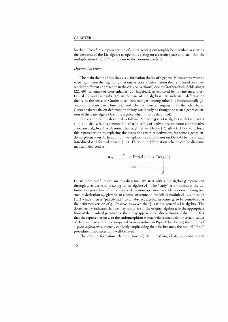
Our version can be described as follows. Suppose g is a Lie algebra with Lie bracket〈·, ·〉 and that ρ is a representation of g in terms of derivations on some commutativeassociative algebra A with unity, that is, ρ : g → Der(A) ⊂ gl(A). Now we deformthis representation by replacing the derivations with σ-derivations for some algebra en-domorphism σ on A. In addition, we replace the commutator on Der(A) by the alreadyintroduced σ-deformed version (1.1). Hence our deformation scheme can be diagram-matically depicted as:

gρ // Der(A) ///o/o/o Derσ(A)

g

“limit”

kk

Let us more carefully explain this diagram. We start with a Lie algebra g representedthrough ρ as derivations acting on an algebra A. The “curly” arrow indicates the de-formation procedure of replacing the derivation operators by σ-derivations. Taking onesuch σ-derivation ∂σ gives us an algebra structure on the left A-module A · ∂σ through(1.1) which then is “pulled-back” to an abstract algebra structure g, to be considered asthe deformed version of g. Observe, however, that g is not in general a Lie algebra. Thedotted arrow indicates that we may not arrive at the original algebra g in the appropriatelimit of the involved parameters: there may appear some “discontinuities” due to the factthat the representation ρ or the endomorphism σ may behave strangely for certain valuesof the parameters. All this compelled us to introduce in Paper E (see below) the notion ofa quasi-deformation, thereby explicitly emphasizing that, for instance, the natural “limit”procedure is not necessarily well-behaved.

The above deformation scheme is (one of ) the underlying idea(s) common to and

10

connecting the chapters of this thesis. The papers on which the chapters are based, con-cerns different aspects and quasi-deformations of Lie algebras, focusing mainly on thespecific examples: the Heisenberg Lie algebra, the Witt and Virasoro algebras and sl2(F).

We now proceed with a thorough description of each Chapter including some back-ground material, historical comments and references.

Chapter 2 (Paper A)

The harmonic oscillator model in physics is perhaps one of the most important modelsin the modern quantum era. In its simplest form (one space dimension) it is given bytwo operators a (annihilation operator) and a† (creation operator) acting on a certaincomplex Hilbert space of states and satisfying the canonical commutation relation

[a, a†] = aa† − a†a = c, (1.3)

where c is some operator commuting with a and a†. These two operators are canonicallyrelated to position x and momentum p, so in a certain representation a = c d

dx anda† = mx, the multiplication (by x) operator3. This representation is often called thecanonical representation of the harmonic oscillator. The vector space

h3 := Fx⊕ Fy ⊕ Fc

is a Lie algebra under the commutator bracket

[y,x] = yx− xy = c, (1.4)

and where c is central, i.e., [x, c] = [y, c] = 0. The Lie algebra h3 is called the three-dimensional Heisenberg Lie algebra or the oscillator algebra. The algebra spanned by a, a†

and c with bracket (1.3) is a particular representation of h3. The universal envelopingalgebra of h3 can be viewed as the quotient algebra

U(h3) = Fx,y, c/(yx− xy − c, xc− cx, yc− cy), (1.5)

of the free polynomial algebra Fx,y, c by the two-sided ideal generated by the ele-ments yx− xy− c, xc− cx and yc− cy. Now, the Heisenberg (–Weyl) algebra4 H isdefined as

H := U(h3)/(c− 1).

The relation yx− xy = 1 in this algebra is called the Heisenberg canonical commutationrelation and is connected to the famous Heisenberg uncertainty principle in quantum

3We ignore all physical constants such as mass and the Planck constant ~ which technically should be presentwhen considering these things in a physical context.

4This is actually also the first Weyl algebra A1(F), hence the name.

11

CHAPTER 1.

mechanics. Elements of H are simply polynomials over F in x and y which, due to therelation yx − xy − 1, can be put on the normal form

∑i,j αijxiyj , αij ∈ F. We

consider H as the non-commutative polynomial algebra

H = Fx,y,1/(yx− xy − 1).

Usually Fx,y,1 is written Fx,y without explicitly writing out the identity 1. Wewill follow this practice from here on. The assignments y 7→ d

dx and x 7→ mx clearlydefine a representation of H in terms of differential operators on the algebra of polyno-mials. This representation will be most important in Chapter 2 (Paper A) since this is therepresentation which is used to deform the Heisenberg algebra H by replacing the oper-ator d/dx by the Jackson q-derivative (see below) according to our deformation schemedescribed earlier. The only difference is that the Heisenberg algebra is not a Lie algebraso there is no commutator involved to be deformed as well. It is then noted that there isan algebra for which the deformed operator and mx is a particular representation. Thisalgebra is the quotient of the free algebra Fx,y by a deformed version of the Heisen-berg canonical commutation relation. Let us elaborate on this.

We form the q-deformed Heisenberg algebra by the following quotient

Hq := F[q]A,B/(AB − qBA− 1).

A priori q can be transcendental (i.e., non-algebraic over F) but most often one considersq ∈ F. In this case we simply have

Hq := FA,B/(AB − qBA− 1)

and this is the viewpoint we shall take in this thesis. Observe that in any case q is assumedto commute withA andB. The algebra Hq can be naturally represented by the followingoperators A 7→ Dq and B 7→ mx where

Dq(f)(x) =tq(f)(x)− f(x)

(q − 1)x=f(qx)− f(x)

(q − 1)x,

the Jackson q-derivative (see [24], for instance), and tq is the multiplicative translationoperator defined by tq(f)(x) := f(qx).

Burchnall–Chaundy theory and algebraic curves

We here recall the absolute basics of algebraic curves and Burchnall–Chaundy theory.

An algebraic curve can be defined on all levels of abstractions but we choose the mostdown-to-earth definition which is suitable for our constructions in Chapter 2. So, an

12

algebraic curve in F2 = F × F (where F does not have to have zero characteristic) is theset Z of points (u, v) in F2 such that there is a bivariate irreducible polynomial F (x, y)annihilating these points, i.e., F (u, v) = 0.

In 1922 and 1928 J.L. Burchnall and T.W. Chaundy published two papers [9, 10]where a connection between commuting differential operators and algebraic curves wasdiscovered. These papers went unnoticed for almost fifty years when the main resultswere rediscovered in the context of integrable systems [28, 29, 35]. Since the 1970’s,deep connections between algebraic geometry and solutions of non-linear differentialequations have been revealed, indicating an enormous richness, largely still waiting tobe explored, in the intersection where (non-linear) differential equations and algebraicgeometry meet. Not only is this interesting for its own theoretical beauty but also sincenon-linear differential equations appear naturally in a large variety of applications.

To state Burchnall and Chaundy’s main theorem we start off with two commutingdifferential operators

P :=∑

i

pi(t)∂i, Q :=∑

i

qi(t)∂i

where pi, qi are analytic functions in t and ∂ := ddt (we assume here and in what fol-

lows for Chapter 2 that F = C). The assumption that P and Q commute puts severerestrictive conditions on the functions pi and qi.

Theorem 1.1 (Burchnall–Chaundy, version 1). Let P and Q be two commuting differ-ential operators with analytic coefficients in the complex domain. Then there is a bivariatepolynomial F (x, y) ∈ C[x, y] such that F (P,Q) = 0.

The polynomial appearing in this theorem is oftentimes referred to as the Burchnall–Chaundy polynomial. The following is a reformulation of their main result for operatorswith polynomial coefficients.

Theorem 1.2 (Burchnall–Chaundy, version 2). Let P andQ be two commuting elementsin H, the Heisenberg algebra. Then there is a bivariate polynomial F (x, y) ∈ C[x, y] suchthat F (P,Q) = 0.

Actually, their result is even stronger than stated above in version one. They actu-ally produce an algorithmic procedure involving a certain determinant to calculate anexplicit polynomial F annihilating the operators. The pairs of eigenvalues (u, v) ∈ C2

corresponding to the same eigenfunction, i.e., corresponding to the same ψ such that

Pψ = uψ and Qψ = vψ,

lie on the curve Z defined by F (x, y), that is, F (u, v) = 0. Furthermore, there isa “dictionary” between certain geometric and analytic data [35]. For instance, given a

13

CHAPTER 1.

curve Z defined by F (x, y) and two commuting differential operators P and Q satis-fying F (P,Q) = 0, one can construct the common eigenfunctions of P and Q as thesections of a certain line bundle on the (one-point) compactification Z of Z.

The starting point of Chapter 2 is an analogue of the Burchnall–Chaundy theorem(as given in version 2 above) to the q-deformed Heisenberg algebra Hq, due to Hellströmand Silvestrov [24], namely:

Theorem 1.3 (Hellström–Silvestrov). Let P and Q be two commuting elements in Hq.Then there is a bivariate polynomial F (x, y) ∈ Z(Hq)[x, y], with coefficients in the centerof Hq, such that F (P,Q) = 0.

The center of Hq is trivial if q is not a root of unity, i.e., Z(Hq) = C1. However,when qn = 1 for some n > 1 then the center is

Z(Hq) = C[Ad, Bd],

where d is the minimal integer such that qd = 1. Unfortunately the proof of Theorem 1.3as given in [24] is purely existential5. An initial conjecture would be that the determinantscheme devised by Burchnall and Chaundy could be used to calculate the polynomial evenin the case of Hq. This problem is what Chapter 2 (Paper A) is devoted to, by providingexamples indicating that the classical Burchnall–Chaundy method could indeed be usedto generate an annihilating algebraic curve.

Observe that a full proof of the conjecture that this adaption is possible for all ele-ments of Hq is not yet within reach. A natural hope would obviously be to try a directgeneralization of the classical proof of Burchnall and Chaundy. The main reason why ananalogous proof for q-difference operators (i.e., elements in Hq) is problematic is that thesolution space is not as well-behaved as for ordinary differential operators and the proof ofthe classical Burchnall–Chaundy theorem relies heavily on considerations of the solutionsto the eigenvalue-problems for the differential operators P and Q. Therefore a rigorousproof of the possibility of adapting the determinant argument relying on purely algebraicmethods is desirable even though this seems at the moment to be a complicated problem.

Chapter 3 (Paper B)

Investigating the Lie algebra of derivations (or differential operators) on an algebraic vari-ety, scheme or differential manifold has turned out to be a very important and in generalvery difficult problem. However, in one of the simplest algebraic-geometric cases thestructural characteristics of the Lie algebra of derivations is both well-known and muchstudied from many different aspects.

5However, the construction made in the proof actually provides an algorithm for producing the q-Burchnall–Chaundy polynomials, but says essentially nothing theoretically of their form or properties.

14

Consider then the real algebraic curve u2 + v2 = 1 in R2, i.e., the real unit-circle S1.Then functions f on S1 can be interpreted as functions in θ where 0 ≤ θ ≤ 2π. A vectorfield on S1 can be written as f(θ) d

dθ . The vector space of all complex-valued C∞-vectorfields (i.e., with smooth f ) on S1 is denoted by Vect(S1) and is a complex infinite-dimensional Lie algebra under the commutator bracket. Considering only polynomialvector fields, i.e., vector fields f(θ) d

dθ where f is a complex Laurent polynomial, we getthe Witt algebra, d [19, 26].

We see that the Witt algebra d can be identified with the C-vector space spanned bydn := −tn+1 d

dt | n ∈ Z acting on Laurent polynomials in t, and

d =⊕n∈Z

C · dn

with Lie bracket defined by

[dn, dm] = dndm − dmdn = (n−m)dn+m.

This is an infinite-dimensional complex Z-graded Lie algebra. Equivalently, the Wittalgebra d can be viewed as the derivations on the algebra of Laurent polynomials C[t, t−1]and so

Der(C[t, t−1]) = C[t, t−1] · ddt. (1.6)

To say that this algebra is important would be a serious understatement.The Witt algebra is the basic undeformed algebra appearing in Chapter 3 (Paper B).

But in order to have enough on our feet we need to know in more detail the modulestructure of the space of σ-derivations Derσ(A) on a commutative associative algebra A

with unity. It turns out that (see Theorem 3.2 in Chapter 3) if A is a unique factorizationdomain (UFD) and σ 6= id an algebra endomorphism, then Derσ(A) is a cyclic leftA-module, i.e., it can be generated as a left A-module by a single element. Notice thecondition that σ 6= id. An analogous theorem for derivations (i.e., when σ = id) is false,since for instance, rk(Der(C[x, y])) = 2 (where ’rk’ denotes the rank of a module) eventhough C[x, y] is a UFD. The above mentioned Theorem was in fact proven in a moregeneral setting and the reader is referred to Theorem 3.2 in Chapter 3 for the precisestatement and proof.

This means in particular, since the algebra of Laurent polynomials F[t, t−1] is a UFD,that there is a ∂σ ∈ Derσ(F[t, t−1]) such that

Derσ(F[t, t−1]) = F[t, t−1] · ∂σ.

Compare this with (1.6).Now, we come to one of the most important results appearing in this thesis, in the

sense that this will be the machine that produces many of the main examples of the

15

CHAPTER 1.

algebraic structures defined throughout the text. Without stating the theorem explicitly toavoid being caught in technicalities at this stage, we briefly describe its contents. The mainpoint is that there is a skew-symmetric bracket product on the left A-module Derσ(A)defined by

〈a · ∂σ, b · ∂σ〉σ := (σ(a) · ∂σ) (b · ∂σ)− (σ(b) · ∂σ) (a · ∂σ),

where a, b ∈ A, generalizing the commutator for derivations. This product satisfies

〈a · ∂σ, b · ∂σ〉σ = (σ(a)∂σ(b)− σ(b)∂σ(a)) · ∂σ,

in addition to the Jacobi-like identity

a,b,c

〈σ(a) · ∂σ, 〈b · ∂σ, c · ∂σ〉σ〉σ + δ · 〈a · ∂σ, 〈b · ∂σ, c · ∂σ〉σ〉σ

= 0,

where δ ∈ A and a,b,c denotes cyclic summation with respect to a, b, c ∈ A.It is important to notice, however, that the results as stated are dependent on addi-

tional technical assumptions which we have not mentioned. See Theorem 3.3 in Chapter3 for the full statement and assumptions.

From this theorem we can construct a plethora of analogues of the Witt algebra d.For instance, taking A = F[t, t−1] as in the classical case, but using a σ different fromthe identity leads to a σ-deformed Witt algebra. The most general endomorphism onF[t, t−1] is one on the form σ(t) = qts for s ∈ Z and q ∈ F∗ := F \ 0. In Section3.3 we investigate the thus formed algebra in detail. Taking s = 1 we get a q-deformedWitt algebra dq with relations

• 〈dn, dm〉 = qndndm − qmdmdn = (nq − mq)dn+m and

• n,m,k (qn + 1)〈dn, 〈dm, dk〉〉 = 0

where nq denotes the q-number nq := 1+ q+ q2 + · · ·+ qn−1. (See Sections 3.3.1and 3.3.2.) Another possibility is to change the underlying algebra A, which in a senseroughly corresponds to changing the basic geometric object (in the case of d this objectis S1), in addition to σ. (See Section 3.3.3 and the subsection of Section 3.3.2 entitledGeneralization to several variables.) In this way we get a broad class of Witt-like algebraswithin our construction.

The Witt algebra d has a one-dimensional central extension in the category of Liealgebras, namely the Virasoro algebra, Vir, [26]. In fact, the Witt algebra is sometimes,primarily in the physics literature, called the centerless Virasoro algebra6. What do wemean by “one-dimensional central extension”? In short, and slightly simplified, supposeg is a Lie algebra and a an abelian Lie algebra, i.e., 〈a, a〉a = 0, then a central extension

6A curious fact is that Miguel Virasoro himself never considered the algebra now bearing his name, butactually the centerless Virasoro algebra, i.e., the Witt algebra!

16

of g by a is the vector space g′ := g⊕ a endowed with a Lie structure 〈·, ·〉g′ such that ais central in g′, that is, such that 〈g′, a〉g′ = 〈a, g′〉g′ = 0. When a is one-dimensionalwe speak of a one-dimensional central extension. This means that as a vector space Vir isVir = d ⊕ Fc, for c a central (in Vir) basis for a. To be precise, the Virasoro algebra isgenerated as a vector space by the set dnn∈Z ∪ c with relations

• [dn, dm] = (n−m)dn+m + m3−m12 δn+m,0c

• [dn, c] = 0, with n ∈ Z.

For more on extensions see the description of Chapter 4 in this Introduction.The Virasoro algebra appeared in physics in the very first hesitant breaths of string

theory, back when string theory was simply a toy description of the strong interaction, theso-called Veneziano model. As now is well-known and part of history, this model failedits initial aim, but found new life in another direction when it was realized that it actuallyincluded gravity. Roughly speaking, the Witt algebra d can be thought of as a “classical”algebra and the Virasoro algebra then enters when one tries to quantize a classical theoryinvolving d, thereby creating an extra central element c, also called the conformal anomalyor central charge [13, 16, 18].

We should also mention that the Virasoro algebra has two super-symmetric analogues,namely the Neveu–Schwarz algebra and the Ramond algebra. Both of these are infinite-dimensional Lie superalgebras generated (as vector spaces) by elements Li, Yji,j ∪cbut where the Neveu–Schwarz algebra takes the j-indices in 1

2 + Z then for the Ramondalgebra j ∈ Z. These generators should obviously be subject to some Virasoro-like (andZ2-graded) relations but we refrain from giving them (see [34] for instance) since thesealgebras will not appear in this thesis.

The q-deformed Witt algebra dq is an example of an algebraic structure which we callhom-Lie algebra, introduced in Chapter 3 (Paper B) and which includes Lie algebras asa special subclass. We refer to Definition 3.4 in Section 3.2.3 for the formal definition.More examples are provided in the Examples section of Chapter 3. In Section 3.2.4 wedevelop the theory of category-preserving central extensions for hom-Lie algebras with aview toward constructing a q-deformed Virasoro algebra with dq as base algebra. When qis not a root of unity7 such a hom-Lie algebra central extension is shown to exist and beunique (in a certain sense). This algebra is Virq := dq ⊕ Fc, for a central charge c, withrelations

• 〈Virq, c〉 = 〈c,Virq〉 = 0 and

• 〈dn, dm〉 = (nq−mq)dn+m + δn+m,0q−m

6(1+qm)m−1qmqm+1qc.

7When speaking of roots of unity we assume that F is such that it includes the all these relevant roots ofunity. If the reader prefers, think of F as C.

17

CHAPTER 1.

Obviously, when q = 1 we retain the classical Virasoro algebra. The case when q is annth-root of unity is not yet investigated but we suspect that instead of a unique hom-Lie algebra central extension we get in effect several inequivalent ones. In fact, not evenexistence is at all clear. To clarify this is obviously a very important project for the future.

Chapter 4 (Paper C)

Some of the more general examples appearing in Chapter 3 derived from Theorem 3.3do not satisfy the condition for being a hom-Lie algebra. As an example, take for instancethe σ-deformed Witt algebra with σ(t) = qts, s 6= 0, 1. The deformed Jacobi identitytells us that this is in fact not a hom-Lie algebra. However, realizing the importance ofconsidering such general deformations stemming from Theorem 3.3 we introduce themore inclusive notion of a quasi-hom-Lie algebra, which was later expanded (in PaperD) to the even more general and natural quasi-Lie algebras. Without venturing intothe precise definition (which can be found in Chapter 4, Definition 4.1 and 4.3) weformulate these definitions as follows. Let V be a vector space and α, β ∈ L(V ), whereL(V ) denotes the space of linear maps on V . Then a quasi-Lie algebra is an algebrastructure 〈·, ·〉 on V such that

• 〈x, y〉 = ω(x, y)〈y, x〉 and

• x,y,z θ(z, x)〈α(x), 〈y, z〉〉+ β〈x, 〈y, z〉〉

= 0

for ω, θ : Dω, Dθ ⊆ V × V → L(V ). A quasi-hom-Lie algebra is the structure obtainedwhen ω = θ and additionally the condition 〈α(x), α(y)〉 = β α〈x, y〉 is imposed, i.e.,one may say that “α is a β-deformed algebra morphism”.

That these definitions encompass the structures derived from Theorem 3.3 follows bytaking β = δ and ω(x, y) = θ(x, y) = − id for all x, y ∈ V .

It is also shown in Chapter 4 that this definition also includes color Lie algebras, andthus in particular, Lie superalgebras. In short (the complete formal definition can befound in Chapter 4), a color Lie algebra is a Γ-graded vector space, with Γ an abeliangroup, endowed with a bracket multiplication 〈·, ·〉 and a “bi-character” ε : Γ×Γ → F∗such that for homogeneous elements x, y: 〈x, y〉 = −ε(γx, γy)〈y, x〉, where γx, γy ∈ Γdenotes the graded degree of x and y, and the Jacobi-like identity

ε(γz, γx)〈x, 〈y, z〉〉+ ε(γx, γy)〈y, 〈z, x〉〉+ ε(γy, γz)〈z, 〈x, y〉〉 = 0

holds. This is a quasi-hom-Lie algebra with ε = ω = θ. For the Lie superalgebra case Γis Z2 and ε = −ω = −θ = (−1)γxγy .

Contrary to popular belief within the “Lie-theory congregation” which confesses tothe faith that color Lie algebras were introduced by Rittenberg and Wyler in [37] andsubsequently molded into its present form by Scheunert [39] in the late seventies, colorLie algebras seem to have appeared first in a paper by Rimhak Ree in 1960 [36] (and

18

in a special case in a paper by Pierre Cartier in the 50’s) under the name generalized Liealgebras of type χ. Here χ is the commutation factor which we denoted by ε. Indeed,some of the results appearing in Scheunert’s paper [39] are already stated and proved byRee in [36], for example a version of the Poincaré–Birkhoff–Witt theorem.

Since color Lie algebras include as a special case Lie superalgebras and hence thealgebras describing supersymmetries, i.e., the fact that physical particles are either bosons(integer spin) or fermions (half-integer spin), it is natural to ask whether general colorLie algebras can be given any physical meaning. This is indeed the case. At least in asense. The term “color” seems to originate from the paper by Rittenberg and Wyler [37]wherein is remarked that one of the examples which they study include the realization ofthe color charge of quarks as “parafields”. Even today some attention is payed color Liealgebras in connection with “parastatistics”, i.e., (quantum) systems of paraparticles.

Back to Chapter 4. We also provide an example of a deformed loop algebra. Tobe exact, let g be a quasi-hom-Lie algebra. Then the “loopification” of this algebra g isg := g ⊗F F[t, t−1]. We show in Chapter 4 that this is also a quasi-hom-Lie algebrawith natural morphisms α, β and ω. In the Lie algebra case the loop algebra is a specialcase of a construction known as current algebras, which are constructed as follows [19].Suppose that g is a Lie algebra and that T is any topological space. Then the currentalgebra associated to g is the Lie algebra of continuous maps T → g with Lie bracketdefined by

〈f, g〉(x) := 〈f(x), g(x)〉g.

Taking T = S1 and restricting to polynomial maps gives us the loop algebra of g. Noticethe similarities between the loop and Witt algebras.

The really serious work to which Chapter 4 is devoted is to develop a central extensiontheory for the category of quasi-hom-Lie algebras. We write ’a’ central extension theorybecause there could actually be more than one way of constructing a category of quasi-hom-Lie algebras, depending on the choice one makes for what is to be meant by aquasi-hom-Lie algebra morphism. A different choice could result in a different extensiontheory. The choice we have made here is, in our opinion, the natural or canonical one,but someone else might disagree.

Suppose g and a are quasi-hom-Lie algebras with a abelian, that is, 〈a, a〉a = 0. Thenwe define a quasi-hom-Lie algebra central extension of g by a to be a short exact sequence

0 // a ι // Epr // g // 0

in the category of quasi-hom-Lie algebras. The extension is called central if in addition

〈a, E〉E = 〈E, a〉E = 0.

Since the above sequence is in particular a short exact sequence of vector spaces it followsfrom basic homological algebra (“a short exact sequence of projective modules split”) that

19

CHAPTER 1.

there is a linear map (of vector spaces) s : g → E, called a section, such that pr s = idg

(compare with sheaf or vector bundle theory). Then it is easy to show that

〈s(x), s(y)〉E = s〈x, y〉g + ι g(x, y)

for some bilinear map g : g × g → a. It is noted in Chapter 4 that this map satisfies ageneralized skew-symmetry condition as well as a generalized Lie algebra 2-cocycle con-dition. By analogy of the Lie algebra case we call such bilinear g’s 2-cocycle-like maps. SeeSection 4.4 for details.

We prove in Chapter 4 two theorems giving necessary and sufficient conditions forquasi-hom-Lie algebra central extensions. Included are also as examples the verificationsthat the developed central extension theory reduces to the classical cases of Lie algebrasand color Lie algebras, as well as the theory of hom-Lie algebra central extensions asdeveloped in Chapter 3, when making the necessary restrictions to the wanted category.In addition to this we discuss necessary conditions for a given quasi-hom-Lie algebra g tohave an “affinization”, i.e., conditions for the loop algebra to g to have a central extension.

Besides being developed in greater generality than for hom-Lie algebras the quasi-hom-Lie algebra central extension theory is here supplemented with an analogue of theclassical result for Lie algebras saying that there is a one-to-one correspondence betweenequivalences (a notion we explicitly define for quasi-hom-Lie algebras) of extensions ofg by a and classes in the second cohomology group H2(g, a). This problem is not con-sidered in Chapter 3 (Paper B). Note however that we do not develop a full cohomologytheory for quasi-hom-Lie algebras, so a rigorous definition of “second cohomology group”(or in particular that it actually comes with a group structure) is not included. But theanalogy is so strong that we are compelled viewing the appearing elements as cohomology-like classes. In fact, it might be possible to derive the complete set of cohomology relationsfrom what we have already shown, thereby getting a full cohomology theory, but this ishighly uncertain at present.

We should also point out that the central extensions we consider are category-pre-serving, i.e., we extend within the category of quasi-hom-Lie algebras. An interestingthing would be to study extensions in some larger category. For instance, suppose g is ahom-Lie algebra and that g is rigid in this category, that is, has only trivial extensions. Isit possible to find an extension of g in the larger category of quasi-hom-Lie algebras?

Chapter 5 (Paper E)

A complex finite-dimensional semi-simple Lie algebra contains a number of copies of thesimple Lie algebra sl2(C) via the so-called root space decomposition [38]. Also, any Liealgebra can be decomposed as the sum of a semi-simple subalgebra and a solvable sub-algebra (Levi decomposition). This means that in order to fully understand Lie algebrasone needs to study both the semi-simple and the solvable Lie algebras. Of these, the classof semi-simple Lie algebras is by far the simplest and most studied [25]. Therefore to

20

study the deformation theory (in our sense) for general finite-dimensional Lie algebras, afirst natural step would obviously be to study this theory when applied to sl2(C) and thisis to what Chapter 5 (Paper E) is mainly devoted.

In the Cartan–Weyl basis e, f, h, sl2(F) can be written as

〈h, e〉 = 2e, 〈h, f〉 = −2f, 〈e, f〉 = h (1.7)

where Fh is the Cartan subalgebra. The standard two-dimensional matrix representationof sl2(F) satisfying these relations is

e 7→(

0 10 0

), f 7→

(0 01 0

), h 7→

(1 00 −1

)from which is clear that sl2(F), viewed as the linear Lie algebra of the linear Lie groupSL2(F), is the algebra of 2× 2-matrices of trace zero.

Another, and from our point of view, crucial representation is the following in termsof first-order differential operators acting on some algebra A of functions in a variable t:

e 7→ ∂, f 7→ −t2 · ∂, h 7→ −2t · ∂.

It is easy to check that these first-order differential operators (derivations) satisfy relations(1.7) with the indicated substitutions, and so define a representation of sl2(F).

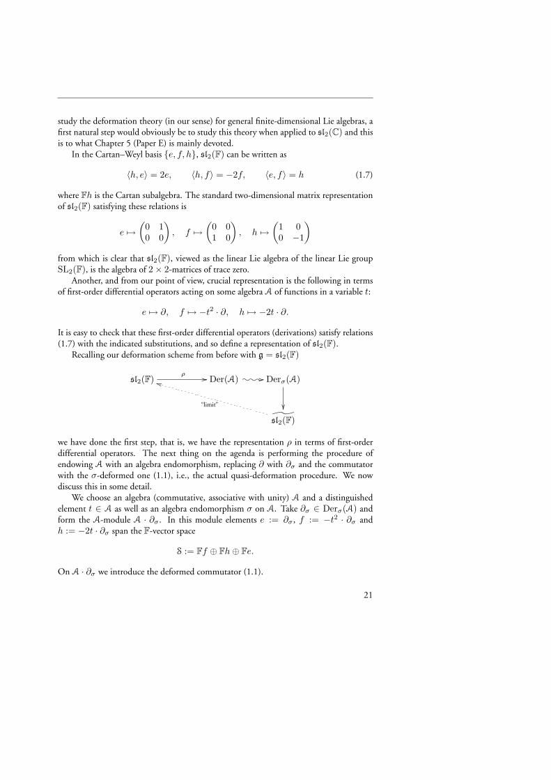
Recalling our deformation scheme from before with g = sl2(F)

sl2(F)ρ // Der(A) ///o/o/o Derσ(A)

sl2(F)

“limit”

kk

we have done the first step, that is, we have the representation ρ in terms of first-orderdifferential operators. The next thing on the agenda is performing the procedure ofendowing A with an algebra endomorphism, replacing ∂ with ∂σ and the commutatorwith the σ-deformed one (1.1), i.e., the actual quasi-deformation procedure. We nowdiscuss this in some detail.

We choose an algebra (commutative, associative with unity) A and a distinguishedelement t ∈ A as well as an algebra endomorphism σ on A. Take ∂σ ∈ Derσ(A) andform the A-module A · ∂σ . In this module elements e := ∂σ , f := −t2 · ∂σ andh := −2t · ∂σ span the F-vector space

S := Ff ⊕ Fh⊕ Fe.

On A · ∂σ we introduce the deformed commutator (1.1).

21

CHAPTER 1.

At this point one is faced with a problem. For general σ and ∂σ this deformedcommutator, restricted from A · ∂σ to S, need not be closed, i.e., 〈S, S〉 * S. It is true,by (1.2), that 〈A · ∂σ,A · ∂σ〉 ⊆ A · ∂σ , but since we do not consider the whole A · ∂σ

only a certain linear subspace S, closure of S under the bracket (1.1) is not apparent, oreven true in general. The best we can do in general is the non-closed expressions

〈h, f〉 = 2σ(t)∂σ(t)t∂σ,

〈h, e〉 = −2(σ(t)∂σ(1)− σ(1)∂σ(t))∂σ,

〈e, f〉 = −(σ(1)(σ(t) + t)∂σ(t)− σ(t)2∂σ(1))∂σ.

Notice that the right-hand-sides do not involve e, f or h, already this quite strange. How-ever, there is a partial remedy, at the cost of absolute generality. More precisely, assumingthat non-negative integer powers of the distinguished element t are linearly independent,we can assume that σ(1) = 1 (or σ(1) = 0, but we consider this uninteresting since thenσ(tw) = 0 for all w ∈ N) and following from this ∂σ(1) = 0. The above formulas thensimplify to

〈h, f〉 = 2σ(t)∂σ(t)t∂σ

〈h, e〉 = 2∂σ(t)∂σ

〈e, f〉 = −(σ(t) + t)∂σ(t)∂σ.

Still, we are obviously not quite there yet. We need to specify more, for instance thealgebra A.

By taking A = F[t] we can explicitly describe those σ and ∂σ such that we haveclosure of S under the bracket. This leads to three different cases to study which is donein Section 5.3.1. Despite not venturing into details we still want to wet the reader’sappetite by sketching the following example which we find particularly interesting.

Example 1. Choosing σ(t) = qt and ∂σ(t) = p0 we obtain an analogue or quasi-deformation of sl2(F) based on the Jackson q-derivative which we recall is defined as

f(t) 7→ Dq(f)(t) := p0f(qt)− f(t)

(q − 1)t.

Remember that when q = 1 and p0 = 1 we retain the ordinary derivative. On theone hand considering the resulting algebra as a skew-symmetric algebra with abstractmultiplication 〈·, ·〉 we get from (1.2):

〈h, f〉 = −2p0qf, 〈h, e〉 = 2p0e, 〈e, f〉 =q + 1

2p0h. (1.8)

Notice that for q = 1, p0 = 1 we get the structure constants for sl2(F) as we should. On

22

the other hand, combining (1.1) and (1.2) we get (q 6= 0):

hf − qfh = −2p0f

he− q−1eh = 2q−1p0e (1.9)

ef − q2fe =q + 1

2p0h

which can be seen as relations in the three abstract generators e, f, h. From this pointof view we thus have the algebra Uq := Fe, f, h/(1.9), where Fe, f, h is the freepolynomial algebra on three generators e, f, h over F. Clearly, Uq is an analogue (or“deformation”) of the universal enveloping algebra for sl2(F), in the sense that for q = 1we get the defining relations for U(sl2(F)).

This algebra is studied in some detail in Chapter 5. For instance we show that Uq

is isomorphic to an iterated Ore extension of the polynomial algebra F[z], and so isAuslander-regular (a definition can be found in Chapter 5, Section 5.3.1). This propertyis rather technical but is very useful since it seems that many of the Auslander-regularalgebras can be viewed as “coordinate rings” for non-commutative schemes and thus in-timately connected to non-commutative algebraic geometry. Also, we note that thereis a PBW-basis, i.e., the monomials eif jhk, for i, j, k ≥ 0, span Uq and are linearlyindependent over F. Moreover, there is a Casimir-like element Ωq in Uq satisfyingΩq · z = τ(z) · Ωq for some automorphism τ . In the Lie case q = 1 we get the or-dinary central Casimir element for U(sl2(F)) in the basis e, f, h.

A much studied, but different from Uq, deformation of U(sl2(C)) is the “quan-tum group” Uq(sl2(C)). Relevant literature for those who want to learn more aboutquantum groups and quantized enveloping algebras are [12, 17, 33] and the extremelywell-written introduction by Christian Kassel [27]. The main point of divergence be-tween Uq(sl2(C)) and Uq is that Uq(sl2(C)) is a quasi-triangular Hopf algebra (i.e., aquantum group according to a modern and almost by-all-accepted definition). It is cer-tainly possible that Uq can be endowed with a Hopf algebra, and further, quasi-triangular,structure, but this is not clear at the moment. This is obviously an important path ofinvestigation for the future. The fact that Uq(sl2(C)) is a Hopf algebra makes it partic-ularly interesting to mathematicians and physicists. The reasons for this are too compli-cated to address here. Suffice it to say that Hopf algebras touch upon (or rather, crashinto) C∗-algebras [33], knot theory [27], affine Lie algebras [17], quantum (conformal)field theory [17, 33], monoidal categories [27], non-commutative geometry [12], grouptheory [33], Lie–Poisson theory [12], ad infinitum...

Back to the thesis. Chapter 5 contains, among other things, a complete descriptionof the algebras appearing as a result of our quasi-deformation scheme in the cases whenA = F[t] and A = F[t]/(t3). In each of these two cases several subcases appear as a resultof different ways to restrict σ and ∂σ to obtain closure of the bracket multiplication.

For all cases we give explicitly the deformed Jacobi identity, which follows in a straight-forward manner from our general theory.

23

CHAPTER 1.

When A = F[t]/(t3), the relations become, where σ(t) = 1 + q1t + q2t2 and

∂σ(t) = p0 + p1t+ p2t2,

q1hf + 2q2f2 − q21fh = −2q1p0f

q1he+ 2q2fe− eh = 2p0e− p1h− 2p2f

ef − q21fe = (p1 + q1p1 + q2p0)f +q1 + 1

2p0h.

(1.10)

The condition ∂σ(t3) = 0 has to be imposed which leads to p0(q21 + q1 + 1) = 0. Sowe need to consider the separate cases where p0 = 0 and q21 + q1 + 1 = 0. If p0 6= 0we obviously have that q1 has to be a third root of unity. So we may view this case as a“generation of deformations at the third roots of unity”. The resulting algebra is of thesame type as (1.9), i.e., the relations are the same, at least when specifying the parametersas p1 = p2 = q2 = 0 in (1.10). In fact, this can be generalized easily, to generatedeformations at N th-roots of unity by considering instead A = F[t]/(tN ). If, instead,p0 = 0 then the defining relations above can be written (assuming q1 6= 0)

hf − q1fh = −2q2/q1f2

q1he− eh = −p1h− 2p2f − 2q2fe

ef − q21fe = p1(1 + q1)f.

(1.11)

Notice that sl2(F) cannot be recovered from this deformation by choosing the parameterssuitably. Taking p1 = p2 = 0, q1 = 1 and putting ε := −2q2, the first relation in (1.11)become the defining relation for the so-called Jordanian quantum plane.

The Jordanian quantum plane is the non-commutative two-dimensional space with“coordinate ring”

Jε := Fx, y/(xy − yx− εy2).

Notice that we get the ordinary commutative coordinate ring for F2 in the limit ε→ 0.Also, J1, is one of two possible Artin–Schelter regular algebras in global dimension

two8. The other one, is the ordinary quantum plane Fx, y/(xy − qyx). Withoutventuring into the precise definition (see Chapter 5, Section 5.3.1 for this) we can roughlydescribe Artin–Schelter regular (AS-regular) algebras as non-commutative analogues ofhomogeneous coordinate rings for smooth projective varieties. This motivates the use ofAS-regular algebras as base algebras for non-commutative projective spaces, often called“quantum Pn’s” [1, 2, 3, 4].

Another example appearing in the subcase defined by (1.11) is the universal envelop-ing algebra for the three-dimensional Heisenberg Lie algebra h3:

h3 := Fx⊕ Fy ⊕ Fc, [x,y] = c, [x, c] = [y, c] = 0.8We should point out that, in fact, Jε

∼= J1 for all ε 6= 0. This follows by performing the base changex 7→ εx and y 7→ y.

24

This can be seen by putting q1 = 1, p1 = q2 = 0 and p2 = −1/2 in (1.11). There arein fact other Lie algebras appearing in subcase (1.11). This is the family la of solvable Liealgebras with relations

hf − fh = 0, he− eh = −h− af, ef − fe = f, a ∈ F.

It is interesting to notice that the subcase that “generates” all the above Lie algebrasfail to generate sl2(C). Hence it is reasonable to think that this is somehow connected tothe moduli theory for three-dimensional Lie algebras where sl2(C) sits alone and cannotbe deformed into the other algebras. Obviously this is a very important issue that needsto be clarified for the full understanding of three-dimensional quasi-Lie algebras.

25

CHAPTER 1.

26

Bibliography

[1] Artin, M., Schelter, W., Graded Algebras of Global Dimension 3, Adv. Math. 66(1987), 171–216.

[2] Artin, M., Tate, J., Van den Bergh, M., Some Algebras Associated to Automorphismsof Elliptic Curves, The Grothendieck Festschrift Vol 1, 33–85, Birkhauser, Boston(1990).

[3] Artin, M., Tate, J., Van den Bergh, M., Modules over regular algebras of dimension 3,Invent. Math. 106 (1991), 335–388.

[4] Artin, M., Zhang, J.J., Noncommutative Projective Schemes, Adv. Math. 109 no. 2(1994), 228-287.

[5] Bell, A.D., Smith, S.P., Some 3-dimensional Skew Polynomial Rings, Preprint, Draftof April 1, 1997.

[6] Bjar, H., Laudal, O.A., Deformations of Lie algebras and Lie algebras of deformations,Compositio Math. 75 (1990), no 1, 69–111.

[7] Björk, J.-E., Rings of Differential Operators, North-Holland, 1979, 374 pp.

[8] Björk, J.-E., Analytic D-Modules and Applications, Kluwer Acad. Publishers, 1993,581 pp.

[9] Burchnall, J.L., Chaundy, T.W., Commutative ordinary differential operators, Proc.London Math. Soc. (Ser. 2), 21 (1922), 420–440.

[10] Burchnall, J. L., Chaundy, T. W., Commutative ordinary differential operators, Proc.Roy. Soc. London A 118 (1928), 557–583.

[11] Cartan, H., Eilenberg, S., Homological Algebra, Princeton University Press, 1956,390 pp.

[12] Chari V., Pressley A., A guide to Quantum Groups, Cambridge University Press,1995, 651 pp.

[13] Di Francesco, P., Mathieu, P., Sénéchal, D., Conformal Field Theory, Springer Verlag,1997, 890 pp.

27

BIBLIOGRAPHY

[14] Ekström, E.K., The Auslander condition on graded and filtered noetherian rings, Sémi-naire Dubreil–Malliavin 1987-88, LNM 1404, Springer Verlag, 1989, 220–245.

[15] Fialowski, A., Deformations of Lie algebras, Eng. Trans. Math. USSR-Sbornik 55:2(1986), 467–473.

[16] Frenkel, I., Lepowsky, J., Meurman, A., Vertex Operator Algebras and the Monster,Academic Press, 1988, 508 pp.

[17] Fuchs, J., Affine Lie Algebras and Quantum Groups, Cambridge University Press,1992, 433 pp.

[18] Fuchs, J., Lectures on Conformal Field Theory and Kac-Moody Algebras, Springer Lec-ture Notes in Physics 498, 1997, 1–54. @arxiv.org: hep-th/9702194.

[19] Fuks, D.B., Cohomology of Infinite-Dimensional Lie Algebras, Plenum PublishingCorp., 1986, 339 pp.

[20] Gerstenhaber, M., On the deformation of rings and algebras, I, III, Ann. of Math. 79(2) (1964), 59–103, 88 (2) (1968), 1–34.

[21] Gorbatsevich, V.V., Onishchik, A.L., Vinberg, E.B., Structure of Lie Groups and LieAlgebras in Encyclopedia of Math. Sciences Vol. 41, Springer-Verlag 1994, 248 pp.

[22] Harris, J., Morrison, I., Moduli of curves, Graduate Texts in Mathematics 187,Springer-Verlag New York, 1998, 366 pp.

[23] Hartshorne, R., Algebraic Geometry, Graduate Texts in Mathematics 52, Springer-Verlag New York, 1977, 496 pp.

[24] Hellström L., Silvestrov, S.D., Commuting Elements in q-Deformed Heisenberg Alge-bras, World Scientific, 2000, 256 pp.

[25] Humphreys, J.E., Introduction to Lie algebras and representation theory, GraduateTexts in Mathematics 9 Springer-Verlag New York-Berlin, 1978, 171 pp.

[26] Kac, V.G., Raina, A.K., Highest weight representations of infinite-dimensional Lie al-gebras, World Scientific, 1987, 145 pp.

[27] Kassel, C., Quantum groups, Graduate Texts in Mathematics 155, Springer-VerlagNew York, 1995, 531 pp.

[28] Krichever, I. M., Integration of non-linear equations by the methods of algebraic geom-etry, Funktz. Anal. Priloz. 11, 1 (1977), 15–31.

[29] Krichever, I. M., Methods of algebraic geometry in the theory of nonlinear equations,Uspekhi Mat. Nauk 32, 6 (1977), 183–208.

28

BIBLIOGRAPHY

[30] Laksov, D., Thorup, A., These are the differential of order n, Trans. Amer. Math. Soc.351 (1999), no 4, 1293-1353.

[31] Lang, S., Algebra, Addison-Wesley, 2nd edition, 1984, 714 pp.

[32] Laudal, O.A., Noncommutative algebraic geometry, Rev. Mat. Iber. 19 (2003), no 2,509–580.

[33] Majid, S., Foundations of Quantum Groups, Cambridge University Press, PaperbackEdition 2000, 640 pp.

[34] Meurman, A., Rocha-Caridi, A., Highest Weight Representions of the Neveu–Schwarzand Ramond Algebras, Commun. Math. Phys. 107 (1986), 263–294.

[35] Mumford, D., An algebro-geometric construction of commuting operators and of solu-tions to the Toda lattice equation, Korteweg–de Vries equation and related non-linearequations, Proc.Int. Symp. on Algebraic Geometry, Kyoto (1978), 115–153.

[36] Ree, R., Generalized Lie elements, Canad. J. Math. 12 (1960), 493–502.

[37] Rittenberg, V., Wyler, D., Generalized Superalgebras, Nucl. Phys. B. vol 13 Issue 3,(1978), 189–202.

[38] Serre, J.P., Complex semisimple Lie Algebras, Springer, 2001, 74 pp.

[39] Scheunert, M., Generalized Lie Algebras, J. Math. Phys. 20 (1979), no 4, 712–720.

[40] Schlessinger, M., Functors of Artinian Rings, Trans. Amer. Math. Soc. 130 (1968),No. 2, 208–222.

[41] Van Oystaeyen, F., Algebraic Geometry for Associative Algebras, Marcel Dekker, 2000,287 pp.

[42] Weibel, C.A., Introduction to homological algebra, Cambridge University Press, 1995,448 pp.

29

BIBLIOGRAPHY

30

Chapter 2

Burchnall–Chaundy theory ofq-Difference operators and q-deformedHeisenberg algebras

This Chapter is based on:

• Larsson, D., Silvestrov, S.D., Burchnall-Chaundy Theory for q-Difference Operatorsand q-Deformed Heisenberg Algebras, J. Nonlinear Math. Phys. 10, Supplement 2(2003), 95–106.

Note: In this Chapter the underlying field will be an algebraically closed field of charac-teristic zero, denoted by C.

2.1 Introduction

One of the major achievements in the theory of non-linear differential equations is thealgebraic-geometric method, relating integrable non-linear differential equations and theirsolutions to properties of algebraic curves and algebraic manifolds. It was originally de-veloped in 1970’s in connection to the inverse scattering problem [18, 19, 20, 21, 22, 23,24, 25, 26, 27, 28, 29, 30], but since then it has become an area of research on its own,greatly influencing developments in algebraic geometry, non-linear equations and algebra,as well as playing an increasingly important role in many applications. This interplay be-tween algebraic geometry and integrable non-linear equations is based on the observationthat many of these equations can be formulated as conditions on the coefficients of somedifferential operators equivalent to the property that these operators commute. Thus themain problem becomes to describe, as detailed as possible, commuting differential oper-ators. The solution of this problem is where algebraic geometry enters the scene. Themain result responsible for this connection was obtained by Burchnall and Chaundy inthe beginning of the 1920’s and further explored by them in a series of papers over thefollowing decade [2, 3, 4]. This key result states that commuting differential operatorssatisfy an equation for a certain algebraic curve, which can be explicitly calculated for eachpair of commuting operators. This correspondence has also been discretized to classicaldifference operators [22, 24, 25]. However not so much has been done in this directionfor q-difference operators, in spite of their widespread applications and long and colorfulhistory. Only recently have some results appeared in the direction of integrable non-linear

31

CHAPTER 2.

q-difference equations [1, 6, 7, 8, 9, 10, 17]. In [11], the key Burchnall–Chaundy typetheorem for q-difference equations was obtained, where it was stated as a corollary toa more general theorem of this type for q-deformed Heisenberg algebras. The proof in[11] is an existence argument, which can be used successfully for an algorithmic imple-mentation for computing the corresponding algebraic curves. However, since it does notgive any specific information on the structure or properties of such algebraic curves, it isdesirable to have a way of describing such algebraic curves by some explicit formulae. Inthis article we make a step in that direction by offering a number of interesting examples,a rigorous, general, proof yet to be completed.

Jackson q-derivative and q-difference operators

This section is devoted to ordinary q-difference operators and q-difference equations, thatis, to q-difference operators and q-difference equations in spaces of functions of a singlevariable t.

In 1908 F. H. Jackson [12, 13, 14, 15, 16] re-introduced and started a systematicstudy of the q-difference operator

(Dqa) (t) =a(qt)− a(t)

(q − 1)t, q 6= 1, (2.1)

which is now sometimes referred to as Euler–Jackson or Jackson q-difference operatoror simply the q-derivative. This operator may be applied without any problems to anyfunction not containing t = 0 in the domain of definition. By definition, the limit as qapproaches 1 is the ordinary derivative, that is

limq→1

(Dqa) (t) =dadt

(t), (2.2)

if a is differentiable at t. The Dq-constants or multiplicatively q-periodic functions aresolutions of the functional equation

k(qt) = k(t) or Dqk(t) = 0. (2.3)

These functions play in the theory of q-difference equations the role of the arbitraryconstants of the differential equations.

The formulas for the q-difference of a sum of functions and of a product by a constantare [5]:

Dq (a(t) + b(t)) = Dqa(t) +Dqb(t), (2.4)

Dq (γ · a(t)) = γ ·Dqa(t), for γ ∈ C. (2.5)

So the operator Dq is linear when it acts on a linear space of functions, and the generaltheory of linear operators developed within linear algebra, functional analysis, operatortheory and operator algebras can be applied.

32

2.1. INTRODUCTION

The formulas for the q-difference of a product and a quotient of functions are [5]:

Dq (a(t)b(t)) = a(qt)Dqb(t) +Dqa(t)b(t), (2.6)

Dq

(a(t)b(t)

)=b(t)Dqa(t)− a(t)Dqb(t)

b(qt)b(t). (2.7)

The usual Leibniz rule for q-derivative is recovered from (2.6) as q → 1.The q-analogue of the chain rule is more complicated since it involves q-derivatives

for different values of q depending on the composed functions. For example if b(t) is thefunction b(t) : t 7→ γ · tk and qk 6= 1, then

Dq(a b)(t) =(Dqk(a)

)(b(t))Dq(b)(t). (2.8)

The chain rule for general b(t) and a(t) is

Dq(a b)(t) = D b(qt)b(t)

(a)(b(t)) ·Dq(b)(t) (2.9)

If b(t) and a(t) are interpreted not as formal expressions but as functions, then thisformula is true for all t 6= 0 such that b(t) 6= 0 and b(qt) 6= b(t), with other points trequiring separate consideration. The general chain rule (2.9) is easily proved as follows:

Dq(a b)(t) =a(b(qt))− a(b(t))

(q − 1)t=a( b(qt)

b(t) b(t))− a(b(t))

( b(qt)b(t) − 1)b(t)

( b(qt)b(t) − 1)b(t)

(q − 1)t=

= D b(qt)b(t)

(a)(b(t)) ·Dq(b)(t).

Strangely enough, we have not been able to find this formula and the above easy proofexplicitly anywhere in the literature on q-analysis.

The general Leibniz rule for action of powers of the q-derivative operator on a productof functions is

Dnq (ab)(t) =

n∑k=0

(n

k

)q

Dkq (a)(tqn−k)Dn−k

q (b)(t) (2.10)

Using the multiplicative q-shift operator tq : a(t) 7→ a(qt) the Leibniz rules (2.6) and(2.10) can be written as follows:

Dq (a(t)b(t)) = tqa(t)Dqb(t) +Dqa(t)b(t), (2.11)

Dnq (ab)(t) =

n∑k=0

(n

k

)q

tn−kq Dk

q (a)(t)Dn−kq (b)(t). (2.12)

33

CHAPTER 2.

Here we have used the q-binomial coefficients defined by(n

k

)q

=nq!

kq!n− kq!(2.13)

for k = 0, 1, . . . , n, where

nq =n∑

k=1

qk−1, 0q = 0, (2.14)

nq! =n∏

k=1

kq, 0q! = 1. (2.15)

are the q-analogues of the natural numbers and the factorial function. The q-binomialcoefficients

(nk

)q

are polynomials in q with integer coefficients. If q = 1, then nq = n.If q 6= 1, then nq = (qn − 1)/(q − 1).

It can be easily checked from the definition of the q-derivative that the action of Dq

on the functions ts is given by the q-analogue of the usual rule

Dq(ts) = sqts−1.

The linear q-difference operators, which use Jackson q-derivative operator Dq as the gen-erator, are sums of the form

P =n∑

j=0

pjDjq,

where the coefficients pi are some functions, which we assume in this article for simplicityof exposition to be polynomials in t.

2.2 A Burchnall–Chaundy type theorem

The q-deformed Heisenberg algebra for q ∈ C \ 0 is a C-algebra Hq with unit el-ement 1 and generators A and B satisfying defining q-deformed Heisenberg canonicalcommutation relation

AB − qBA = 1. (2.16)

The algebra can be constructed as the quotient

Hq :=CA,B

(AB − qBA− 1)

of the free algebra CA,B by the two-sided ideal generated by AB − qBA− 1.

34

2.2. A BURCHNALL–CHAUNDY TYPE THEOREM

The q-deformed Heisenberg algebra is fundamental for q-difference equations, dueto the fact that the Jackson q-difference operator Dq and the operator of multiplicationmt : a(t) 7→ t · a(t) satisfy the q-deformed Heisenberg canonical commutation relation

Dqmt − q ·mtDq = 1. (2.17)

Indeed,

(Dqmt − q ·mtDq)(a)(t) =qta(qt)− ta(t)

(q − 1)t− qta(qt)− qta(t)

(q − 1)t=

=qta(t)− ta(t)

(q − 1)t= a(t) = (1a)(t)

In the terminology of representation theory this means that the operators Dq and mt arerepresentatives of generators in the representation of the q-deformed Heisenberg algebraHq. Any pair, or more generally, a set of linear operators satisfying some commuta-tion relations is also called a representation of these commutation relations. So, the pair(Dq,mt) is a representation of the q-deformed Heisenberg commutation relation (2.16).Any algebraic identity which holds in Hq results in the corresponding identity for the op-erators Dq and mt, thus having an impact on the related q-difference equations.

Using the defining commutation relations (2.16) it can be checked that

B2A2 = q−1BA(BA− 1)

B3A3 = q−3BA(BA− 1)(BA− (q + 1)1).

An inductive argument gives

BnAn = q−n(n−1)

2

n−1∏j=0

(BA− (

j−1∑k=0

qk)1)

= q−n(n−1)

2

n−1∏j=0

(BA− jq1

). (2.18)

Using this we see, for example, that

B4A4 = q−6BA(BA− 1)(BA− (q + 1)1)(BA− (q2 + q + 1)1) =

= q−6BA(BA− 1q1)(BA− 2q1)(BA− 3q1).

From the equality (2.18) we get the following very useful fact.

Lemma 2.1. In the q-deformed Heisenberg algebra Hq, all monomials, and linear combi-nations of monomials, of the form BnAn commute.

The following theorem is a generalization of the Burchnall–Chaundy theorem to q-deformed Heisenberg algebras. The general algebraic way this result is stated is importantbecause then the property becomes universal in its nature, being consequently applica-ble not only to q-difference operators arising from the specific representation (Dq,mt),but also to any other class of operators associated to any other representation of the q-deformed Heisenberg canonical commutation relation.

35

CHAPTER 2.

Theorem 2.2 (Hellström, Silvestrov [11]). If P,Q ∈ Hq commute, i.e., PQ = QP ,then there exists a nonzero polynomial F in two commutative variables with coefficients fromthe center Z(Hq) of Hq such that F (P,Q) = 0 in Hq.

The center Z(Hq) of Hq is the set of elements in Hq commuting with any elementin Hq. If q is not a root of unity or if q = 1, then the center of Hq is trivial, thatis consisting only from the elements of the form λ1, λ ∈ C. So in this case, to anypair of commuting elements in Hq, one can associate an algebraic curve in C2 given bythe corresponding polynomial with coefficients in C, the existence of which is stated inTheorem 2.2. In the case when q is a root of unity but not 1, the center of Hq is thesubalgebra generated by Ad and Bd where d is the smallest positive integer such thatqd = 1. The coefficients in the polynomial from the theorem are some elements of thiscommutative subalgebra. They might be the elements of the form λ1, and in this case weagain would get an ordinary algebraic curve. But if they are not, then we get an algebraiccurve with coefficients, which are not scalars but polynomials in Ad and Bd. However,in a particular representation we might still get ordinary algebraic curves as some or allcentral elements might become, for example, scalar multiples of the identity operator.

The proof of Theorem 2.2 given in [11] is an existence proof based on dimensiongrowth arguments. Though it can be used for construction of an algorithm for computingthe annihilating polynomials for the given pair of commuting elements in Hq, it does notgive any specific formula for such polynomials that could lead to a better understandingof their structure and of the interplay with algebraic geometry.

In the classical case of differential operators, that is in the case of H1, there is a way toconstruct the annihilating algebraic curves via determinants, going back to Burchnall andChaundy [2, 3, 4]. An extension of this construction to general q-difference operatorsis not yet available but believed to be possible in some generality. Here we would likeinstead to give some new interesting examples strongly indicating that the determinantswork well also in the q-deformed case. These examples also provide a good illustrationfor the general method.

Before we turn to the examples let us first review the classical Burchnall–Chaundyconstruction for differential operators. Let P =

∑ni=0 pi(t)∂i and Q =

∑mi=0 qi(t)∂

i

be two differential operators of degree n and m respectively, where functions pi(t) andqi(t) are analytic in their common domain of definition, or just formal power series,or as in all examples in this article, polynomials in t with coefficients in C. The orig-inal Burchnall–Chaundy theorem states, informally, that two commuting differentialoperators P and Q lie on an algebraic curve, in the sense that they are annihilatedby a polynomial in two variables after being substituted for the variables. One of thefirst consequences of this is that the eigenvalues, corresponding to a joint eigenfunctionof the two operators, are coordinates of a point on that curve. There are also otherdeeper connections of properties of the algebraic curve to properties of the solutionsof the equations associated to these operators, for example the non-linear differentialequations in the coefficient functions, obtained from commutativity of those operators

36

2.2. A BURCHNALL–CHAUNDY TYPE THEOREM

[18, 19, 20, 21, 22, 23, 24, 25, 26, 27, 28, 29, 30].The original proof of Burchnall–Chaundy theorem depends heavily on the existence

of solutions of boundary value problems for ordinary differential equations, making asimple adaption of it to q-difference operators problematic. A beautiful feature of theproof in the differential operator case, however, is that it is constructive in the sense thatit actually tells us how to compute such an annihilating curve, given the commutingoperators. This is done by constructing the resultant (or eliminant) of operators P andQ. We sketch this construction, as it is important to have in mind for this article. Thefollowing row-scheme is a first stepping-stone:

∂k(P − u1) =n+k∑i=0

θi,k∂i − u∂k, k = 0, 1, . . . ,m− 1 (2.19)

∂k(Q− v1) =m+k∑i=0

ωi,k∂i − v∂k, k = 0, 1, . . . , n− 1 (2.20)

where θi,k and ωi,k are certain functions built from the coefficients of P and Q respec-tively, whose exact form is calculated by moving ∂k through to the right of the coeffi-cients, using the Leibniz rule. The coefficients of the powers of ∂ on the right hand sidein (2.19) and (2.20) build up the rows of a matrix exactly as written. That is, as the firstrow we take the coefficients in

∑ni=0 θi,0∂

i − u∂0, and as the second row – the coeffi-cients in

∑n+1i=0 θi,1∂

i − u∂, continuing this until k = m− 1. As the mth row we takethe coefficients in

∑mi=0 ωi,0∂

i− v∂0, and as the (m+1)th row we take the coefficientsin

∑m+1i=0 ωi,1∂

i − v∂ and so on. In this manner we get a (m + n) × (m + n)-matrixusing (2.19) and (2.20). The determinant of this matrix yields a bivariate polynomialF (u, v) in u and v over C (sometimes called the Burchnall–Chaundy polynomial), defin-ing an algebraic curve F (u, v) = 0, and annihilating P and Q when putting u = P andv = Q.

Now, generalizing this idea to the case of q-difference operators, we indicate with anumber of examples, that it is in fact a sound construction even in the q-deformed case.

Example 2. We take P = m3tD

3q and Q = m2

tD2q . Then the following formulae hold:

D0q(P − u1) = −u1 + m3

tD3q ,

Dq(P − u1) = −uDq + 3qm2tD

3q + q3m3

tD4q ,

D0q(Q− v1) = −v1 + m2

tD2q ,

Dq(Q− v1) = −vDq + 2qmtD2q + q2m2

tD3q ,

D2q(Q− v1) = −vD2

q + 2qD2q + (q2q + q22q)mtD

3q + q4m2

tD4q =

= (2q − v1)D2q + q22

qmtD3q + q4m2

tD4q .

37

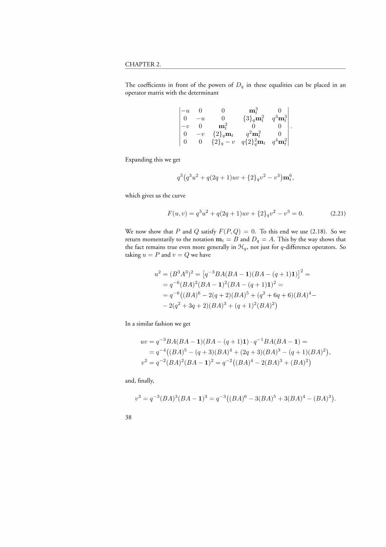
CHAPTER 2.

The coefficients in front of the powers of Dq in these equalities can be placed in anoperator matrix with the determinant

∣∣∣∣∣∣∣∣∣∣−u 0 0 m3

t 00 −u 0 3qm2

t q3m3t

−v 0 m2t 0 0

0 −v 2qmt q2m2t 0

0 0 2q − v q22qmt q4m2

t

∣∣∣∣∣∣∣∣∣∣.

Expanding this we get

q3(q3u2 + q(2q + 1)uv + 2qv

2 − v3)m6

t ,

which gives us the curve

F (u, v) = q3u2 + q(2q + 1)uv + 2qv2 − v3 = 0. (2.21)

We now show that P and Q satisfy F (P,Q) = 0. To this end we use (2.18). So wereturn momentarily to the notation mt = B and Dq = A. This by the way shows thatthe fact remains true even more generally in Hq, not just for q-difference operators. Sotaking u = P and v = Q we have

u2 = (B3A3)2 =[q−3BA(BA− 1)(BA− (q + 1)1)

]2 =

= q−6(BA)2(BA− 1)2(BA− (q + 1)1)2 =

= q−6((BA)6 − 2(q + 2)(BA)5 + (q2 + 6q + 6)(BA)4−

− 2(q2 + 3q + 2)(BA)3 + (q + 1)2(BA)2)

In a similar fashion we get

uv = q−3BA(BA− 1)(BA− (q + 1)1) · q−1BA(BA− 1) =

= q−4((BA)5 − (q + 3)(BA)4 + (2q + 3)(BA)3 − (q + 1)(BA)2

),

v2 = q−2(BA)2(BA− 1)2 = q−2((BA)4 − 2(BA)3 + (BA)2

)and, finally,

v3 = q−3(BA)3(BA− 1)3 = q−3((BA)6 − 3(BA)5 + 3(BA)4 − (BA)3

).

38

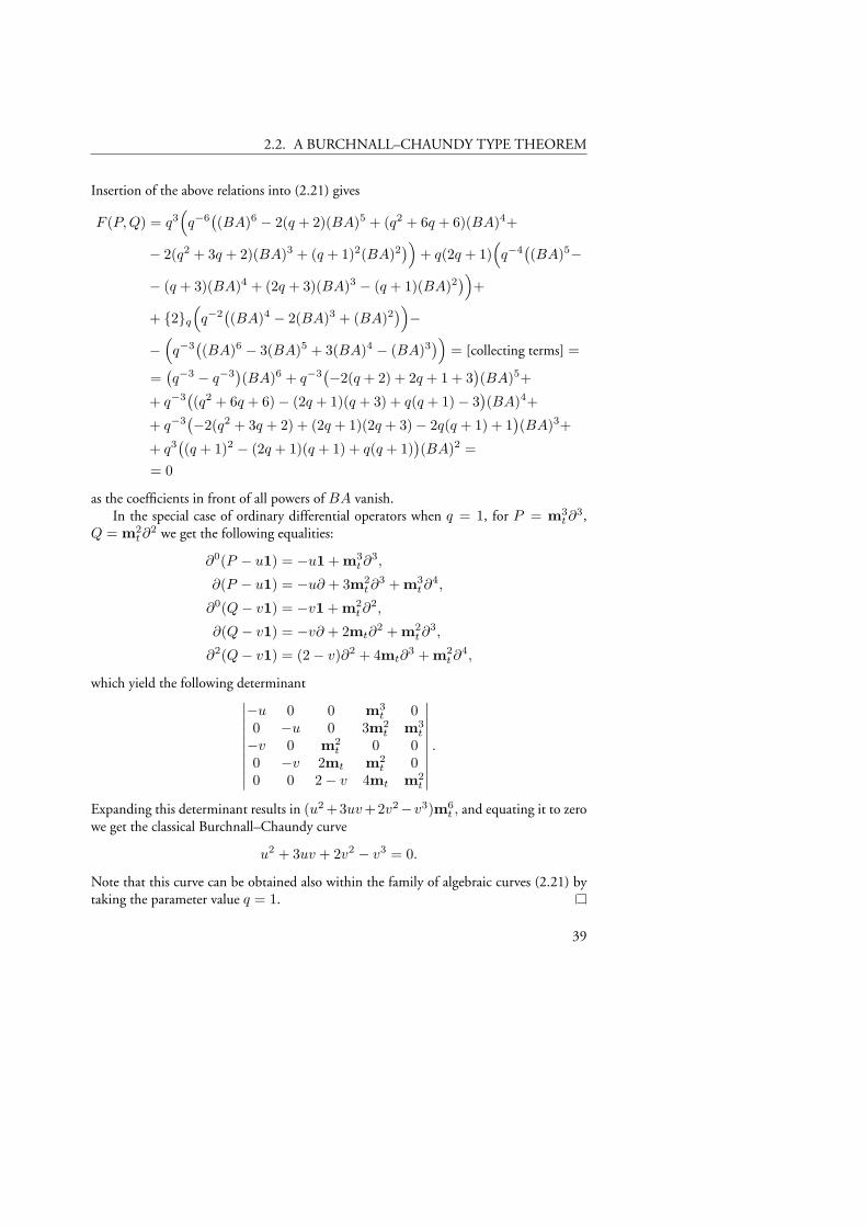
2.2. A BURCHNALL–CHAUNDY TYPE THEOREM

Insertion of the above relations into (2.21) gives

F (P,Q) = q3(q−6

((BA)6 − 2(q + 2)(BA)5 + (q2 + 6q + 6)(BA)4+

− 2(q2 + 3q + 2)(BA)3 + (q + 1)2(BA)2))

+ q(2q + 1)(q−4

((BA)5−

− (q + 3)(BA)4 + (2q + 3)(BA)3 − (q + 1)(BA)2))

+

+ 2q

(q−2

((BA)4 − 2(BA)3 + (BA)2

))−

−(q−3

((BA)6 − 3(BA)5 + 3(BA)4 − (BA)3

))= [collecting terms] =

=(q−3 − q−3

)(BA)6 + q−3

(−2(q + 2) + 2q + 1 + 3

)(BA)5+

+ q−3((q2 + 6q + 6)− (2q + 1)(q + 3) + q(q + 1)− 3

)(BA)4+

+ q−3(−2(q2 + 3q + 2) + (2q + 1)(2q + 3)− 2q(q + 1) + 1

)(BA)3+

+ q3((q + 1)2 − (2q + 1)(q + 1) + q(q + 1)

)(BA)2 =

= 0

as the coefficients in front of all powers of BA vanish.In the special case of ordinary differential operators when q = 1, for P = m3

t∂3,

Q = m2t∂

2 we get the following equalities:

∂0(P − u1) = −u1 + m3t∂

3,

∂(P − u1) = −u∂ + 3m2t∂

3 + m3t∂

4,

∂0(Q− v1) = −v1 + m2t∂

2,

∂(Q− v1) = −v∂ + 2mt∂2 + m2

t∂3,

∂2(Q− v1) = (2− v)∂2 + 4mt∂3 + m2

t∂4,

which yield the following determinant∣∣∣∣∣∣∣∣∣∣−u 0 0 m3

t 00 −u 0 3m2

t m3t

−v 0 m2t 0 0

0 −v 2mt m2t 0

0 0 2− v 4mt m2t

∣∣∣∣∣∣∣∣∣∣.

Expanding this determinant results in (u2 +3uv+2v2−v3)m6t , and equating it to zero

we get the classical Burchnall–Chaundy curve

u2 + 3uv + 2v2 − v3 = 0.

Note that this curve can be obtained also within the family of algebraic curves (2.21) bytaking the parameter value q = 1.

39

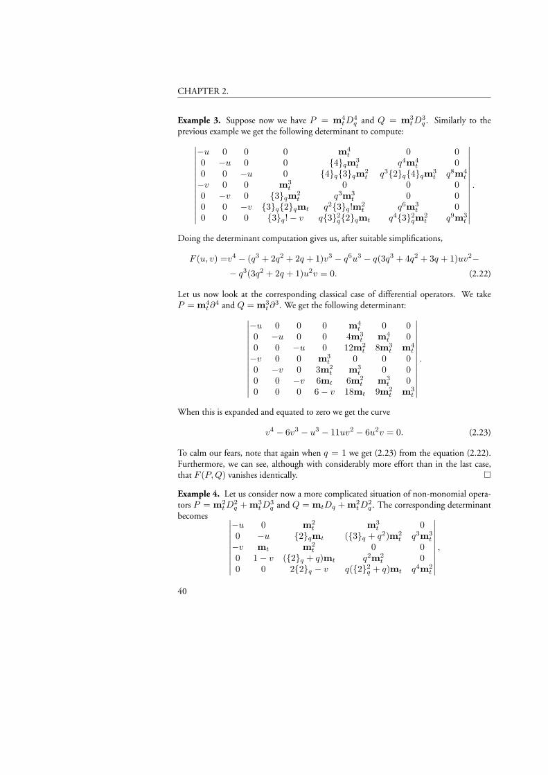
CHAPTER 2.

Example 3. Suppose now we have P = m4tD

4q and Q = m3

tD3q . Similarly to the

previous example we get the following determinant to compute:∣∣∣∣∣∣∣∣∣∣∣∣∣∣

−u 0 0 0 m4t 0 0

0 −u 0 0 4qm3t q4m4

t 00 0 −u 0 4q3qm2

t q32q4qm3t q8m4

t

−v 0 0 m3t 0 0 0

0 −v 0 3qm2t q3m3

t 0 00 0 −v 3q2qmt q23q!m2

t q6m3t 0

0 0 0 3q!− v q32q2qmt q432

qm2t q9m3

t

∣∣∣∣∣∣∣∣∣∣∣∣∣∣.

Doing the determinant computation gives us, after suitable simplifications,

F (u, v) =v4 − (q3 + 2q2 + 2q + 1)v3 − q6u3 − q(3q3 + 4q2 + 3q + 1)uv2−− q3(3q2 + 2q + 1)u2v = 0. (2.22)

Let us now look at the corresponding classical case of differential operators. We takeP = m4

t∂4 and Q = m3

t∂3. We get the following determinant:∣∣∣∣∣∣∣∣∣∣∣∣∣∣

−u 0 0 0 m4t 0 0

0 −u 0 0 4m3t m4

t 00 0 −u 0 12m2

t 8m3t m4

t

−v 0 0 m3t 0 0 0

0 −v 0 3m2t m3

t 0 00 0 −v 6mt 6m2

t m3t 0

0 0 0 6− v 18mt 9m2t m3

t

∣∣∣∣∣∣∣∣∣∣∣∣∣∣.

When this is expanded and equated to zero we get the curve

v4 − 6v3 − u3 − 11uv2 − 6u2v = 0. (2.23)

To calm our fears, note that again when q = 1 we get (2.23) from the equation (2.22).Furthermore, we can see, although with considerably more effort than in the last case,that F (P,Q) vanishes identically.

Example 4. Let us consider now a more complicated situation of non-monomial opera-tors P = m2

tD2q + m3

tD3q and Q = mtDq + m2

tD2q . The corresponding determinant

becomes ∣∣∣∣∣∣∣∣∣∣−u 0 m2

t m3t 0

0 −u 2qmt (3q + q2)m2t q3m3

t

−v mt m2t 0 0

0 1− v (2q + q)mt q2m2t 0

0 0 22q − v q(22q + q)mt q4m2

t

∣∣∣∣∣∣∣∣∣∣,

40

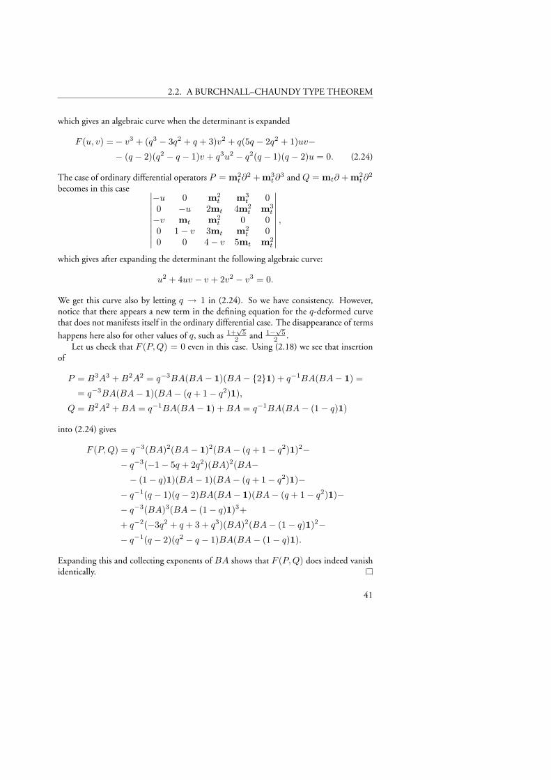
2.2. A BURCHNALL–CHAUNDY TYPE THEOREM

which gives an algebraic curve when the determinant is expanded

F (u, v) =− v3 + (q3 − 3q2 + q + 3)v2 + q(5q − 2q2 + 1)uv−− (q − 2)(q2 − q − 1)v + q3u2 − q2(q − 1)(q − 2)u = 0. (2.24)

The case of ordinary differential operators P = m2t∂

2 + m3t∂

3 and Q = mt∂ + m2t∂

2

becomes in this case ∣∣∣∣∣∣∣∣∣∣−u 0 m2

t m3t 0

0 −u 2mt 4m2t m3

t

−v mt m2t 0 0

0 1− v 3mt m2t 0

0 0 4− v 5mt m2t

∣∣∣∣∣∣∣∣∣∣,

which gives after expanding the determinant the following algebraic curve:

u2 + 4uv − v + 2v2 − v3 = 0.

We get this curve also by letting q → 1 in (2.24). So we have consistency. However,notice that there appears a new term in the defining equation for the q-deformed curvethat does not manifests itself in the ordinary differential case. The disappearance of terms

happens here also for other values of q, such as 1+√

52 and 1−

√5

2 .Let us check that F (P,Q) = 0 even in this case. Using (2.18) we see that insertion

of

P = B3A3 +B2A2 = q−3BA(BA− 1)(BA− 21) + q−1BA(BA− 1) =

= q−3BA(BA− 1)(BA− (q + 1− q2)1),

Q = B2A2 +BA = q−1BA(BA− 1) +BA = q−1BA(BA− (1− q)1)

into (2.24) gives

F (P,Q) = q−3(BA)2(BA− 1)2(BA− (q + 1− q2)1)2−− q−3(−1− 5q + 2q2)(BA)2(BA−− (1− q)1)(BA− 1)(BA− (q + 1− q2)1)−

− q−1(q − 1)(q − 2)BA(BA− 1)(BA− (q + 1− q2)1)−− q−3(BA)3(BA− (1− q)1)3+

+ q−2(−3q2 + q + 3 + q3)(BA)2(BA− (1− q)1)2−− q−1(q − 2)(q2 − q − 1)BA(BA− (1− q)1).

Expanding this and collecting exponents of BA shows that F (P,Q) does indeed vanishidentically.

41

CHAPTER 2.

We would be very interested to get an answer to the following question. Is it truethat the genus of the Burchnall–Chaundy curves resulting from operators mn

t Dnq and

mmt D

mq (and linear combination of these) is always zero irrespective of the value of q

when taken in C \ 0?

42

Bibliography

[1] Adler M., Horozov E., van Moerbeke, P., The solution to the q-KdV equation, Phys.Lett. A. 242, 3 (1998), 139–151.

[2] Burchnall, J. L., Chaundy, T. W., Commutative ordinary differential operators, Proc.London Math. Soc. (Ser. 2) 21 (1922), 420–440.

[3] Burchnall, J. L., Chaundy, T. W., Commutative ordinary differential operators, Proc.Roy. Soc. London A 118 (1928), 557–583.

[4] Burchnall, J. L., Chaundy, T. W., Commutative ordinary differential operators. II. —The Identity Pn = Qm, Proc. Roy. Soc. London A 134 (1932), 471–485.

[5] Exton, H., q-Hypergeometric functions and applications, Ellis Horwood Limited,Chichester (1983).

[6] Frenkel, E., Deformations of the KdV hierarchy and related soliton equations, Internat.Math. Res. Notices 2 (1996), 55–76.

[7] Haine, L., Iliev, P., The bispectral property of q-deformation of Schur polynomials andq-KdV hierarchy, J. Phys. A: Math. Gen. 30, 20 (1997), 7217–7227.

[8] Iliev, P., Solutions to Frenkel’s deformation of the KP hierarchy, J. Phys. A: Math. Gen.31, 12 (1998), L241–L244.

[9] Iliev, P., Tau function solutions to a q-deformation of the KP hierarchy, Lett. Math.Phys. 44, 3 (1998), 187–200.

[10] Iliev, P., Algèbres commutatives d’operateurs aux q-différences et systèmes de Calogero-Moser, C. R. Acad. Sci. Paris, Sér. I 329, 10 (1999), 877–882.

[11] Hellström, L., Silvestrov, S. D., Commuting elements in q-deformed Heisenberg alge-bras, World Scientific (2000), 256 pp.

[12] Jackson, F. H., On q-functions and a certain difference operator, Trans. Roy. Soc. Edin.46 (1908), 253–281.

[13] Jackson, F. H., A q-form of Taylor’s theorem, Mess. Math. 38 (1909), 62–64.

[14] Jackson, F. H., A q-series corresponding to Taylor’s series, Mess. Math. 39 (1909),26–28.

43

BIBLIOGRAPHY

[15] Jackson, F. H., On q-definite integrals, Quart. J. Pure Appl. Math. 41 (1910), 193–203.

[16] Jackson, F. H., q-Difference equations, American J. Math. 32 (1910), 305–314.

[17] Khesin, B., Lyubashenko, V., Roger, C., Extensions and contractions of the Lie algebraof q-pseudodifferential symbols on the circle, J. Funct. Anal. 143, 1 (1997), 55–97.

[18] Krichever, I. M., Algebraic curves and commuting matrix differential operators,Funktz. Anal. Priloz. 10, 2 (1976), 75–76.

[19] Krichever, I. M., Integration of non-linear equations by the methods of algebraic geom-etry, Funktz. Anal. Priloz. 11, 1 (1977), 15–31.

[20] Krichever, I. M., Methods of algebraic geometry in the theory of nonlinear equations,Uspekhi Mat. Nauk 32, 6 (1977), 183–208.

[21] Krichever, I. M., Commutative rings of ordinary linear differential operators, Funktz.Anal. Priloz. 12, 3 (1978), 20–31.

[22] Krichever, I. M., Algebraic curves and non-linear difference equations, Comm.Moscow Math. Soc. 33 (1978), 170-171.

[23] Krichever, I. M., Novikov, S. P., Holomorphic bundles over algebraic curves, and non-linear equations, Uspekhi Mat. Nauk 35, 6 (216) (1980), 47–68.

[24] van Moerbeke, P., Mumford, D., The spectrum of difference operators and algebraiccurves, Acta Mathematica 143 (1979), 93–154.

[25] Mumford, D., An algebro-geometric construction of commuting operators and of solu-tions to the Toda lattice equation, Korteweg–de Vries equation and related non-linearequations, Proc.Int. Symp. on Algebraic Geometry, Kyoto (1978), 115–153.

[26] Veselov, A. P., Hamiltonian formalism for the Novikov–Krichever equations for thecommutativity of two operators, Funktz. Anal. Priloz. 13, 1 (1979), 1–7.

[27] Veselov, A. P., Integrable maps, Uspekhi Mat. Nauk 46, 5 (1991), 3–45.

[28] Wilson, G., Commuting flows and conservation lows for Lax equations, Math. Proc.Camb. Phil. Soc. 86 (1979), 131–143.

[29] Wilson, G., Hamiltonian and algebro-geometric integrals of stationary equations ofKdV type, Math. Proc. Camb. Phil. Soc. 87 (1980), 295–305.

[30] Wilson, G., Algebraic curves and soliton equations, in Geometry Today, (E. Arbarello,C. Procesi, E. Strickland, eds.), Birkhäuser, Boston (1985), 303–329.

44

Chapter 3

Deformations of Lie Algebras usingσ-Derivations

This Chapter is based on the papers:

• Hartwig, J.T., Larsson, D., Silvestrov, S.D., Deformations of Lie algebras using σ-derivations, Journal of Algebra 295 (2006), 314–361.

• Larsson, D., Silvestrov, S.D., Quasi-Lie Algebras, Preprints in Mathematical Sci-ences 2004:30, LUTFMA-5049-2004, to appear in Contemporary Mathematics391 Amer. Math. Soc.

3.1 Introduction

Multiplicative deformations-discretizations of derivatives have many applications in mod-els of quantum phenomena, as well as in analysis of complex systems and processes ex-hibiting complete or partial scaling invariance. The key algebraic property which is sharedby these differential and difference type operators and making them so useful is that theysatisfy some versions of the Leibniz rule explaining how to calculate the operator onproducts given its action on each factor. It is therefore desirable to have a single unifyingdifferentiation theory, which would be concerned with operators of a certain general class,satisfying generalized Leibniz rule and containing as examples the classical differentiationand other well-known derivations and differences.

The infinite-dimensional Lie algebra of complex polynomial vector fields on the unitcircle, the Witt algebra, is an important example in the classical differential and integralcalculus, relating it to topology and geometry, and at the same time responsible for manyof its key algebraic properties. The universal enveloping algebra of the Witt algebra isisomorphic to an associative algebra with an infinite number of generators dj | j ∈ Zand defining relations

[dn, dm] = dndm − dndm = (n−m)dn+m for n,m ∈ Z. (3.1)

The Witt algebra can also be defined as the complex Lie algebra of derivations on thealgebra of Laurent polynomials C[t, t−1] in one variable, that is the Lie algebra of linearoperators D on C[t, t−1] satisfying the ordinary Leibniz rule D(ab) = D(a)b+ aD(b),with commutator taken as the Lie algebra product. This definition will be most importantin this article, as it will be taken as a starting point for generalization of the Witt algebra,

45

CHAPTER 3.

incorporating operators obeying a generalized Leibniz rule twisted by an endomorphism(Definition 3.3).

Important examples of such twisted derivation-type operators, extensively investi-gated in physics and engineering and lying at the foundations of q-analysis, are the Jack-son q-derivative

Dq(a)(t) =a(qt)− a(t)

qt− t

and

mtDq(a)(t) =a(qt)− a(t)

q − 1

acting on C[t, t−1] or various function spaces. It satisfies a σq-twisted (q-deformed)Leibniz rule Dq(ab) = Dq(a)b + σ(a)Dq(b) for the re-scaling automorphism σ givenby σ(a)(t) = tq(a)(t) := a(qt). In this special case our general construction yieldsa natural q-deformation of the Witt algebra which becomes the usual Witt algebra de-fined by (3.1) when q = 1 (Theorem 3.8). This deformation is closely related to theq-deformations of the Witt algebra introduced and studied for instance in the references[1, 6, 7, 11, 13, 14, 22, 38, 39, 40].

However, our defining commutation relations in this case look somewhat different,as we obtained them, not from some conditions aiming to resolve specifically the case ofq-deformations, but rather by choosing C[t, t−1] as an example of the underlying coeffi-cient algebra and specifying σ to be the automorphism σq in our general construction forσ-derivations. By simply choosing a different coefficient algebra or basic σ-derivationone can construct many other analogues and deformations of the Witt algebra. Wedemonstrate this by examples, constructing a class of deformations of the Witt algebraparameterized by integers defining arbitrary endomorphisms of F[t, t−1] (Theorem 3.9),and also by constructing a multi-dimensional analogue of the Witt algebra by taking theunderlying algebra to be Laurent polynomials in several variables F[z±1

1 , z±12 , . . . , z±1

n ]and choosing σ to be an endomorphism mapping z1, . . . , zn into monomials (Theorem3.11). The important feature of our approach is that, as in the non-deformed case, thedeformations and analogues of Witt algebra obtained by various choices of the underlyingcoefficient algebra, of the endomorphism σ and of the basic σ-derivation, are preciselythe natural algebraic structures for the differential and integral type calculi and geometrybased on the corresponding classes of generalized derivation and difference type operators.

The non-deformed Witt algebra has a unique, up to multiplication by a scalar, one-dimensional central Lie algebra extension, the Virasoro Lie algebra. Its universal envelop-ing algebra, also usually called the Virasoro algebra, is the algebra with infinite set ofgenerators dj | j ∈ Z ∪ c and defining relations

[dj , dk] = djdk − dkdj = (j − k)dj+k + δj+k,0112 (j + 1)j(j − 1)c,

[c, dk] = cdk − dkc = 0, for j, k ∈ Z. (3.2)

46

3.1. INTRODUCTION

We develop in this article a framework for the construction of central extensions of de-formed Witt algebras built on σ-derivations. To this end we show first that our generaliza-tion of the Witt algebra to general σ-derivations satisfies skew-symmetry and a generalized(twisted) Jacobi identity (Theorem 3.3). The generalized Jacobi identity (3.23) has sixterms, three of them twisted from inside and the other three twisted on the outside. Thisdefines a class of non-associative algebras with multiplication satisfying skew-symmetryand such generalized Jacobi identities, and containing Lie algebras as the untwisted case.Sometimes the twisting can be put on the inside of all terms of the generalized Jacobiidentity in the same way, and the terms can be coupled to yield the generalized Jacobiidentity with three terms. For example, this is the case for the q-deformation of the Wittalgebra in Theorem 3.8. Armed with this observation we define the corresponding classof non-associative algebras, calling it in this article hom-Lie algebras (Definition 3.4, Sec-tion 3.2.3), since it is associated with a twisting homomorphism. When the twistinghomomorphism is the identity map, the generalized Jacobi identity becomes twice theusual Jacobi identity for Lie algebras, making Lie algebras into an example of hom-Liealgebras. In Section 3.2.4, for the class of hom-Lie algebras, we develop the central exten-sion theory, providing homological type conditions useful for showing existence of centralextensions and for their construction. Here, we required that the central extension of ahom-Lie algebra is also a hom-Lie algebra. In particular, the standard theory of central ex-tensions of Lie algebras becomes a natural special case of the theory for hom-Lie algebraswhen no non-identity twisting is present. In particular, this implies that in the specificexamples of deformation families of Witt and Virasoro type algebras constructed withinthis framework, the corresponding non-deformed Witt and Virasoro type Lie algebras areincluded as the algebras corresponding to those specific values of deformation parameterswhich remove the non-trivial twisting. In Section 3.5, we demonstrate the use of the cen-tral extension theory for hom-Lie algebras by applying it to the construction of a centralhom-Lie algebra extension of the q-deformed Witt algebra from Theorem 3.8, which is aq-deformation of Virasoro Lie algebra. For q = 1 one indeed recovers the usual VirasoroLie algebra as is expected from our general approach.

It should be mentioned that the use of q-deformed Jacobi identities for constructingq-deformations of the Witt and Virasoro algebras has been considered in physical andmathematical literature before [1, 6, 7, 12, 38, 39, 40, 41, 42]. Of these works, the clos-est to our results on hom-Lie algebras comes [1] where the two identities, skew-symmetryand a twisted from inside three-term Jacobi identity, almost as the one for hom-Lie alge-bras, have been clearly stated as a definition of a class of non-associative algebras, and thenused as the conditions required to be satisfied by the central extension of a q-deformationof the Witt algebra from [14]. This results in a q-deformation of the Virasoro Lie algebrasomehow related to that in the example we described in section 3.5. Whether a particu-lar deformation of the Witt or Virasoro algebra obtained by various constructions satisfysome kinds of Jacobi type identities is considered to be an important problem. The gen-eralized twisted 6-term Jacobi identity obtained in our construction, gives automatically

47

CHAPTER 3.

by specialization the deformed Jacobi identities satisfied by the corresponding particulardeformations of the Witt and Virasoro algebras. There are also works employing usualand super Jacobi identities as conditions on central extensions and their deformations (forexample [2, 16, 23, 46]). Putting these works within context of our approach would beof interest.

We would also like to note that in the works [5, 28, 43, 44], in the case of usualderivations on Laurent polynomials, it has been specifically noted that a Lie bracket canbe defined by expressions somewhat resembling a special case of (3.21). We also wouldlike to mention that q-deformations of the Witt and Virasoro algebras were consideredindirectly as an algebra of pseudo q-difference operators based on the q-derivative on Lau-rent polynomials in [21, 22, 25]. We believe that it should be possible, and would be ofdirect interest, to extend the results of these works to our general context of σ-derivations,and we hope to contribute to this cause in future work. For the reader’s convenience, wehave also included in the bibliography, without further reference in the text, some workswe know of, concerned with other specific examples of deformations of Witt algebras thatwe believe could be considered in our framework, leaving the possibility of this as an openquestion for the moment.

We also feel that the further development should include using our construction forbuilding more examples of deformed or twisted Witt and Virasoro type algebras based ondifferential and difference type operators on function spaces studied extensively in anal-ysis and in numerical mathematics, and on functions on algebraic varieties important inalgebraic geometry and its applications. It could be of interest to extend our constructionsand examples over fields of finite characteristic, or various number fields. Developmentof the representation theory for the parametric families of Witt and Virasoro type alge-bras arising within our method, and understanding to which extent the representationsof non-deformed Witt and Virasoro algebras appear as limit points will be important forapplications in physics.

3.2 Some general considerations

3.2.1 Generalized derivations on commutative algebras and UFD’s

We begin with some definitions. By F we denote a field of characteristic zero. Throughoutthis section, A is an associative F-algebra, and σ and τ denote two different algebraendomorphisms on A.

Definition 3.1. A (σ, τ)-derivation ∂(σ,τ) on A is a F-linear map satisfying

∂(σ,τ)(ab) = ∂(σ,τ)(a)τ(b) + σ(a)∂(σ,τ)(b),

where a, b ∈ A. The set of all (σ, τ)-derivations on A is denoted by Der(σ,τ)(A).

48

3.2. SOME GENERAL CONSIDERATIONS

Definition 3.2. A σ-derivation on A is a (σ, id)-derivation, i.e., a F-linear map ∂σ sat-isfying

∂σ(ab) = ∂σ(a)b+ σ(a)∂σ(b),

for a, b ∈ A. We de note the set of all σ-derivations by Derσ(A).

From now on, when speaking of unique factorization domains (UFD), we shall alwaysmean a commutative associative algebra over F with unity 1 and with no zero-divisors,such that any element can be written in a unique way (up to a multiple of an invertibleelement) as a product of irreducible elements, i.e., elements which cannot be written asa product of two non-invertible elements. Examples of unique factorization domainsinclude F[x1, . . . , xn], and the algebra F[t, t−1] of Laurent polynomials.

When σ(x)a = aσ(x) (or τ(x)a = aτ(x)) for all x, a ∈ A and in particular whenA is commutative, Der(σ,τ)(A) carries a natural left (or right) A-module structure by(a, ∂(σ,τ)) 7→ a · ∂(σ,τ) : x 7→ a∂(σ,τ)(x). If a, b ∈ A we shall write a

∣∣b if there is anelement c ∈ A such that ac = b. If S ⊆ A is a subset of A, a greatest common divisor,gcd(S), of S is defined as an element of A satisfying

gcd(S)∣∣a for a ∈ S, (3.3)

and

b∣∣a for a ∈ S =⇒ b

∣∣ gcd(S). (3.4)

It follows directly from the definition that

S ⊆ T ⊆ A =⇒ gcd(T )∣∣ gcd(S) (3.5)

whenever gcd(S) and gcd(T ) exist. If A is a unique factorization domain one can showthat a gcd(S) exists for any nonempty subset S of A and that this element is unique upto a multiple of an invertible element in A. Thus we are allowed to speak of the gcd.

Lemma 3.1. Let A be a commutative algebra. Let σ and τ be two algebra endomorphismson A, and let ∂(σ,τ) be a (σ, τ)-derivation on A. Then

∂(σ,τ)(x)(τ(y)− σ(y)) = 0

for all x ∈ ker(τ − σ) and y ∈ A. Moreover, if A has no zero-divisors and σ 6= τ , then

ker(τ − σ) ⊆ ker ∂(σ,τ). (3.6)

Proof. Let y ∈ A and let x ∈ ker(τ − σ). Then

0 = ∂(σ,τ)(xy − yx) == ∂(σ,τ)(x)τ(y) + σ(x)∂(σ,τ)(y)− ∂(σ,τ)(y)τ(x)− σ(y)∂(σ,τ)(x) == ∂(σ,τ)(x)(τ(y)− σ(y))− ∂(σ,τ)(y)(τ(x)− σ(x)) = ∂(σ,τ)(x)(τ(y)− σ(y)).

Furthermore, if A is an integral domain (i.e., has no zero-divisors) and if there is anelement y ∈ A such that τ(y) 6= σ(y) then ∂(σ,τ)(x) = 0.

49

CHAPTER 3.

Theorem 3.2. Let σ and τ be different algebra endomorphisms on a unique factorizationdomain A. Then Der(σ,τ)(A) is free of rank one as an A-module with generator

∂(σ,τ) :=(τ − σ)

g: x 7−→ (τ − σ)(x)

g(3.7)

where g = gcd((τ − σ)(A)).

Proof. We note first that (τ − σ)/g is a (σ, τ)-derivation on A:

(τ − σ)(xy)g

=τ(x)τ(y)− σ(x)σ(y)

g=

=(τ(x)− σ(x))τ(y) + σ(x)(τ(y)− σ(y))

g=

=(τ − σ)(x)

g· τ(y) + σ(x) · (τ − σ)(y)

g,

for x, y ∈ A. Next we show that (τ − σ)/g generates a free A-module of rank one. Sosuppose that

x · τ − σ

g= 0, (3.8)

for some x ∈ A. Since τ 6= σ, there is an y ∈ A such that (τ − σ)(y) 6= 0. Applicationof both sides in (3.8) to this y yields

x · (τ − σ)(y)g

= 0.

Since A has no zero-divisors, it then follows that x = 0. Thus

A · τ − σ

g

is a free A-module of rank one.It remains to show that Der(σ,τ)(A) ⊆ A · τ−σ

g . Let ∂(σ,τ) be a (σ, τ)-derivationon A. We want to find a′ ∈ A such that

∂(σ,τ)(x) = a′ · (τ − σ)(x)g

(3.9)

for x ∈ A. We will define

a′ =∂(σ,τ)(x) · g(τ − σ)(x)

(3.10)

50

3.2. SOME GENERAL CONSIDERATIONS

for some x such that (τ − σ)(x) 6= 0. For this to be possible, we must show two things.First of all, that

(τ − σ)(x)∣∣ ∂(σ,τ)(x) · g for any x with (τ − σ)(x) 6= 0 (3.11)

and secondly, that

∂(σ,τ)(x) · g(τ − σ)(x)

=∂(σ,τ)(y) · g(τ − σ)(y)

(3.12)

for any x, y ∈ A with (τ − σ)(x), (τ − σ)(y) 6= 0. Suppose for a moment that (3.11)and (3.12) were true. Then it is clear that if we define a′ by (3.10), the formula (3.9)holds for any x ∈ A satisfying (τ −σ)(x) 6= 0. But (3.9) also holds when x ∈ A is suchthat (τ − σ)(x) = 0, because then ∂(σ,τ)(x) = 0 also, by Lemma 3.1.

We first prove (3.11). Let x, y ∈ A be such that (τ − σ)(x), (τ − σ)(y) 6= 0. Thenwe have

0 = ∂(σ,τ)(xy − yx) == ∂(σ,τ)(x)τ(y) + σ(x)∂(σ,τ)(y)− ∂(σ,τ)(y)τ(x)− σ(y)∂(σ,τ)(x) == ∂(σ,τ)(x)(τ(y)− σ(y))− ∂(σ,τ)(y)(τ(x)− σ(x)),

so that

∂(σ,τ)(x)(τ(y)− σ(y)) = ∂(σ,τ)(y)(τ(x)− σ(x)). (3.13)

Now define a function h : A×A → A by setting

h(z, w) = gcd(τ(z)− σ(z), τ(w)− σ(w)) for z, w ∈ A.

By the choice of x and y, we have h(x, y) 6= 0. Divide both sides of (3.13) by h(x, y):

∂(σ,τ)(x)τ(y)− σ(y)h(x, y)

= ∂(σ,τ)(y)τ(x)− σ(x)h(x, y)

. (3.14)

By construction

gcd(τ(y)− σ(y)

h(x, y),τ(x)− σ(x)h(x, y)

)= 1.

Therefore, using that A is a UFD, we deduce from (3.14) that

τ(x)− σ(x)h(x, y)

∣∣ ∂(σ,τ)(x),

implying that

(τ − σ)(x)∣∣ ∂(σ,τ)(x) · h(x, y) (3.15)

51

CHAPTER 3.

for any x, y ∈ A with (τ −σ)(x), (τ −σ)(y) 6= 0. Let S = A\ ker(τ −σ). Then from(3.15) and property (3.4) of the gcd we get

(τ − σ)(x)∣∣ ∂(σ,τ)(x) · gcd(h(x, S)) (3.16)

for all x ∈ A with (τ − σ)(x) 6= 0. But

gcd(h(x, S)) = gcd(gcd

((τ − σ)(x), (τ − σ)(s)

)| s ∈ S

)=

= gcd((τ − σ)(S) ∪ (τ − σ)(x)) == gcd((τ − σ)(A) ∪ (τ − σ)(x)) == g.

Thus (3.16) is equivalent to (3.11) which was to be proved.Finally, we prove (3.12). Let x, y ∈ A be such that (τ − σ)(x), (τ − σ)(y) 6= 0.

Then

0 = ∂(σ,τ)(xy − yx) == ∂(σ,τ)(x)τ(y) + σ(x)∂(σ,τ)(y)− ∂(σ,τ)(y)τ(x)− σ(y)∂(σ,τ)(x) == ∂(σ,τ)(x)(τ(y)− σ(y))− ∂(σ,τ)(y)(τ(x)− σ(x)),

which, after multiplication by g and division by (τ − σ)(x) · (τ − σ)(y) proves (3.12).This completes the proof of the existence of a′, and hence the proof of the theorem.

3.2.2 A bracket on σ-derivations

The Witt algebra is isomorphic to the Lie algebra Der(F[t, t−1]) of all derivations of thecommutative unital algebra of all F-valued Laurent polynomials:

F[t, t−1] = ∑k∈Z

aktk | ak ∈ F, only finitely many non-zero.

In this section we will use this fact as a starting point for a generalization of the Wittalgebra to an algebra consisting of σ-derivations.

We let A be a commutative associative algebra over F with unity 1, as in the exam-ple A = F[t, t−1] from the previous paragraph. When we speak of homomorphisms(endomorphisms) in the sequel we will always mean algebra homomorphisms (endomor-phisms), except where otherwise indicated. If σ : A → A is a homomorphism of alge-bras, we denote, as before, the A-module of all σ-derivations on A by Derσ(A). Forclarity we will denote the module multiplication by · and the algebra multiplication in A

by juxtaposition. The annihilator Ann(∂σ) of an element ∂σ ∈ Derσ(A) is the set ofall a ∈ A such that a · ∂σ = 0. It is easy to see that Ann(∂σ) is an ideal in A for any∂σ ∈ Derσ(A).

52

3.2. SOME GENERAL CONSIDERATIONS

We now fix a homomorphism σ : A → A, an element ∂σ ∈ Derσ(A), and anelement δ ∈ A, and we assume that these objects satisfy the following two conditions:

σ(Ann(∂σ)) ⊆ Ann(∂σ), (3.17)

∂σ(σ(a)) = δσ(∂σ(a)), for a ∈ A. (3.18)

LetA · ∂σ = a · ∂σ | a ∈ A

denote the cyclic A-submodule of Derσ(A) generated by ∂σ . To simplify notation weintroduce a convenient way of writing cyclic sums. If f : A × A × A → A · ∂σ is afunction, we will write

a,b,c f(a, b, c) := f(a, b, c) + f(b, c, a) + f(c, a, b).

We note the following properties of the cyclic sum:

a,b,c

(x · f(a, b, c) + y · g(a, b, c)

)= x· a,b,c f(a, b, c) + y· a,b,c g(a, b, c),

a,b,c f(a, b, c) =a,b,c f(b, c, a) =a,b,c f(c, a, b),

where f, g : A × A × A → A · ∂σ are two functions, and x, y ∈ A. Combining thesetwo identities we obtain

a,b,c

(f(a, b, c) + g(a, b, c)

)=a,b,c

(f(a, b, c) + g(b, c, a)

)=

=a,b,c

(f(a, b, c) + g(c, a, b)

). (3.19)

We now have the following theorem, which introduces a F-algebra structure on A · ∂σ .

Theorem 3.3. If equation (3.17) holds then the map

〈·, ·〉σ : A · ∂σ ×A · ∂σ → A · ∂σ

defined by setting

〈a · ∂σ, b · ∂σ〉σ = (σ(a) · ∂σ) (b · ∂σ)− (σ(b) · ∂σ) (a · ∂σ), (3.20)

for a, b ∈ A, where denotes composition of functions, is a well-defined F-algebra producton the F-linear space A · ∂σ , satisfying the following identities for a, b, c ∈ A:

〈a · ∂σ, b · ∂σ〉σ = (σ(a)∂σ(b)− σ(b)∂σ(a)) · ∂σ, (3.21)

〈a · ∂σ, b · ∂σ〉σ = −〈b · ∂σ, a · ∂σ〉σ. (3.22)

If, in addition (3.18) holds, then

a,b,c

〈σ(a) · ∂σ, 〈b · ∂σ, c · ∂σ〉σ〉σ + δ · 〈a · ∂σ, 〈b · ∂σ, c · ∂σ〉σ〉σ

= 0. (3.23)

53

CHAPTER 3.

We will often omit the ’’ in formulas such as (3.20).

Remark 1. An important thing to notice is that the bracket 〈·, ·〉σ defined in the theoremdepends on the generator ∂σ of the cyclic submodule A · ∂σ of Derσ(A) in an essentialway. This reveals that one should in fact write 〈·, ·〉σ,∂σ

to explicitly indicate which ∂σ ischosen. Suppose, however, we choose another generator ∂′σ of A · ∂σ . Then ∂′σ = u∂σ

for an element u ∈ A (not necessarily a unit). Take elements a · ∂′σ , b · ∂′σ ∈ A · ∂σ .Then the following calculation shows how two different brackets relate when changingthe generator (we use the commutativity of A freely):

σ(u)〈a · ∂′σ, b · ∂′σ〉σ,∂′σ = [The definition of the bracket] == (σ(a)uσ(u) · ∂σ)(bu · ∂σ)− (σ(b)uσ(u) · ∂σ)(au · ∂σ) =

= u ·((σ(au) · ∂σ)(bu · ∂σ)− (σ(bu) · ∂σ)(au · ∂σ)

)=

= u · 〈au · ∂σ, bu · ∂σ〉σ,∂σ= u · 〈a · ∂′σ, b · ∂′σ〉σ,∂σ

so the ”base change”-relation is

σ(u) · 〈a · ∂′σ, b · ∂′σ〉σ,∂′σ = u · 〈a · ∂′σ, b · ∂′σ〉σ,∂σ .

For the most part of this paper, we have a fixed generator and so we suppress the depen-dence on the generator from the bracket notation and simply write 〈·, ·〉σ. On the otherhand, if A has no zero-divisors, we shall see later in Proposition 3.4 that the dependenceof the generator ∂σ is not essential.

Remark 2. The identity (3.21) is just a formula expressing the product defined in (3.20)as an element of A ·∂σ . Identities (3.22) and (3.23) are more essential, expressing, respec-tively, skew-symmetry and a generalized ((σ, δ)-twisted) Jacobi identity for the productdefined by (3.20).

We now turn to the proof of Theorem 3.3.

Proof. We must first show that 〈·, ·〉σ is a well-defined function, that is, if we havea1 · ∂σ = a2 · ∂σ , then

〈a1 · ∂σ, b · ∂σ〉σ = 〈a2 · ∂σ, b · ∂σ〉σ, (3.24)

and

〈b · ∂σ, a1 · ∂σ〉σ = 〈b · ∂σ, a2 · ∂σ〉σ, (3.25)

for b ∈ A. Now a1 ·∂σ = a2 ·∂σ is equivalent to a1−a2 ∈ Ann(∂σ). Therefore, usingthe assumption (3.17), we also have σ(a1 − a2) ∈ Ann(∂σ). Hence

〈a1 · ∂σ, b · ∂σ〉σ − 〈a2 · ∂σ, b · ∂σ〉σ = (σ(a1) · ∂σ)(b · ∂σ)− (σ(b) · ∂σ)(a1 · ∂σ)−− (σ(a2) · ∂σ)(b · ∂σ) + (σ(b) · ∂σ)(a2 · ∂σ) =

= (σ(a1 − a2) · ∂σ)(b · ∂σ)− (σ(b) · ∂σ)((a1 − a2) · ∂σ) = 0,

54

3.2. SOME GENERAL CONSIDERATIONS

which shows (3.24). The proof of (3.25) is analogous.Next we prove (3.21), which also shows that A · ∂σ is closed under 〈·, ·〉σ . Let the

elements a, b, c ∈ A be arbitrary. Then, since ∂σ is a σ-derivation on A we have

〈a · ∂σ, b · ∂σ〉σ(c) = (σ(a) · ∂σ)((b · ∂σ)(c))− (σ(b) · ∂σ)((a · ∂σ)(c)) == σ(a)∂σ(b∂σ(c))− σ(b)∂σ(a∂σ(c)) =

= σ(a)(∂σ(b)∂σ(c) + σ(b)∂σ(∂σ(c))

)− σ(b)

(∂σ(a)∂σ(c) + σ(a)∂σ(∂σ(c))

)=

=(σ(a)∂σ(b)− σ(b)∂σ(a)

)∂σ(c) + (σ(a)σ(b)− σ(b)σ(a))∂σ(∂σ(c)).

Since A is commutative, the last term is zero. Thus (3.21) is true. The skew-symmetryidentity (3.22) is clear from the definition (3.20). Using the linearity of σ and ∂σ , andthe definition of 〈·, ·〉σ , or the formula (3.21), it is also easy to see that 〈·, ·〉σ is bilinear.

It remains to prove (3.23). Using (3.21) and that ∂σ is a σ-derivation on A we get

〈σ(a) · ∂σ, 〈b · ∂σ, c · ∂σ〉σ〉σ = 〈σ(a) · ∂σ, (σ(b)∂σ(c)− σ(c)∂σ(b)) · ∂σ〉σ =

=σ2(a)∂σ(σ(b)∂σ(c)− σ(c)∂σ(b))−

− σ(σ(b)∂σ(c)− σ(c)∂σ(b))∂σ(σ(a))· ∂σ =

=σ2(a)

(∂σ(σ(b))∂σ(c) + σ2(b)∂2

σ(c)− ∂σ(σ(c))∂σ(b)− σ2(c)∂2σ(b)

)−

−(σ2(b)σ(∂σ(c))− σ2(c)σ(∂σ(b))

)∂σ(σ(a))

· ∂σ =

= σ2(a)∂σ(σ(b))∂σ(c) · ∂σ + σ2(a)σ2(b)∂2σ(c) · ∂σ−

− σ2(a)∂σ(σ(c))∂σ(b) · ∂σ − σ2(a)σ2(c)∂2σ(b) · ∂σ−

− σ2(b)σ(∂σ(c))∂σ(σ(a)) · ∂σ + σ2(c)σ(∂σ(b))∂σ(σ(a)) · ∂σ, (3.26)

where σ2 = σ σ and ∂2σ = ∂σ ∂σ . Applying cyclic summation to the second and

fourth term in (3.26) we get

a,b,c

σ2(a)σ2(b)∂2

σ(c) · ∂σ − σ2(a)σ2(c)∂2σ(b) · ∂σ

=

=a,b,c

σ2(a)σ2(b)∂2

σ(c) · ∂σ − σ2(b)σ2(a)∂2σ(c) · ∂σ

= 0,

using (3.19) and that A is commutative. Similarly, if we apply cyclic summation to thefifth and sixth term in (3.26) and use the relation (3.18) we obtain

a,b,c

− σ2(b)σ(∂σ(c))∂σ(σ(a)) · ∂σ + σ2(c)σ(∂σ(b))∂σ(σ(a)) · ∂σ

=

=a,b,c

− σ2(b)σ(∂σ(c))δσ(∂σ(a)) · ∂σ + σ2(c)σ(∂σ(b))δσ(∂σ(a)) · ∂σ

=

= δ· a,b,c

−σ2(b)σ(∂σ(c))σ(∂σ(a)) ·∂σ +σ2(b)σ(∂σ(a))σ(∂σ(c)) ·∂σ

= 0,

where we again used (3.19) and the commutativity of A. Consequently, the only termsin the right hand side of (3.26) which do not vanish when we take cyclic summation are

55

CHAPTER 3.

the first and the third. In other words,

a,b,c 〈σ(a) · ∂σ, 〈b · ∂σ, c · ∂σ〉σ〉σ =

=a,b,c

σ2(a)∂σ(σ(b))∂σ(c) · ∂σ − σ2(a)∂σ(σ(c))∂σ(b) · ∂σ

. (3.27)

We now consider the other term in (3.23). First note that from (3.21) we have

〈b · ∂σ, c · ∂σ〉σ = (∂σ(c)σ(b)− ∂σ(b)σ(c)) · ∂σ

since A is commutative. Using first this and then (3.21) we get

δ · 〈a · ∂σ, 〈b · ∂σ, c · ∂σ〉σ〉σ = δ · 〈a · ∂σ, (∂σ(c)σ(b)− ∂σ(b)σ(c)) · ∂σ〉σ =

= δ(σ(a)∂σ(∂σ(c)σ(b)− ∂σ(b)σ(c))− σ(∂σ(c)σ(b)− ∂σ(b)σ(c))∂σ(a)

)· ∂σ =

= δσ(a)

(∂2

σ(c)σ(b) + σ(∂σ(c))∂σ(σ(b))− ∂2σ(b)σ(c)− σ(∂σ(b))∂σ(σ(c))

)−

−(σ(∂σ(c))σ2(b)− σ(∂σ(b))σ2(c)

)∂σ(a)

· ∂σ =

= δσ(a)∂2σ(c)σ(b) · ∂σ + δσ(a)σ(∂σ(c))∂σ(σ(b)) · ∂σ−

− δσ(a)∂2σ(b)σ(c) · ∂σ − δσ(a)σ(∂σ(b))∂σ(σ(c)) · ∂σ−

− δσ(∂σ(c))σ2(b)∂σ(a) · ∂σ + δσ(∂σ(b))σ2(c)∂σ(a) · ∂σ.

Using (3.18), this is equal to

δσ(a)∂2σ(c)σ(b) · ∂σ + σ(a)∂σ(σ(c))∂σ(σ(b)) · ∂σ−

− δσ(a)∂2σ(b)σ(c) · ∂σ − σ(a)∂σ(σ(b))∂σ(σ(c)) · ∂σ−

− ∂σ(σ(c))σ2(b)∂σ(a) · ∂σ + ∂σ(σ(b))σ2(c)∂σ(a) · ∂σ =

= δσ(a)∂2σ(c)σ(b) · ∂σ − δσ(a)∂2

σ(b)σ(c) · ∂σ−− ∂σ(σ(c))σ2(b)∂σ(a) · ∂σ + ∂σ(σ(b))σ2(c)∂σ(a) · ∂σ.

The first two terms of this last expression vanish after a cyclic summation and using(3.19), so we get

a,b,c δ · 〈a · ∂σ, 〈b · ∂σ, c · ∂σ〉σ〉σ =

=a,b,c

− ∂σ(σ(c))σ2(b)∂σ(a) · ∂σ + ∂σ(σ(b))σ2(c)∂σ(a) · ∂σ

. (3.28)

56

3.2. SOME GENERAL CONSIDERATIONS

Finally, combining this with (3.27) we deduce

a,b,c

〈σ(a) · ∂σ, 〈b · ∂σ, c · ∂σ〉σ〉σ + δ〈a · ∂σ, 〈b · ∂σ, c · ∂σ〉σ〉σ

=

=a,b,c 〈σ(a) · ∂σ, 〈b · ∂σ, c · ∂σ〉σ〉σ+ a,b,c δ〈a · ∂σ, 〈b · ∂σ, c · ∂σ〉σ〉σ =

=a,b,c

σ2(a)∂σ(σ(b))∂σ(c) · ∂σ − σ2(a)∂σ(σ(c))∂σ(b) · ∂σ

+

+ a,b,c

− ∂σ(σ(c))σ2(b)∂σ(a) · ∂σ + ∂σ(σ(b))σ2(c)∂σ(a) · ∂σ

=

=a,b,c

σ2(a)∂σ(σ(b))∂σ(c) · ∂σ − σ2(a)∂σ(σ(c))∂σ(b) · ∂σ

+

+ a,b,c

− ∂σ(σ(b))σ2(a)∂σ(c) · ∂σ + ∂σ(σ(c))σ2(a)∂σ(b) · ∂σ

=

= 0,

as was to be shown. The proof is complete.

Remark 3. There are several other milder assumptions instead of commutativity that willmake the above proof work. Dropping the commutativity does not alter the fact that themapping x · ∂σ : b 7→ x∂σ(b) is a σ-derivation for all x ∈ A and that A · ∂σ is a leftA-module. If

[a, b] ⊆ Ann(∂σ), that is, [a, b] · ∂σ(c) = 0 for all a, b, c ∈ A

then Theorem 3.3 remains valid with the same proof. We only need to note that, althoughA is not commutative we have [a, b] · ∂σ = 0 which is to say that

ab · ∂σ = ba · ∂σ.

We remarked in [26] that also the following conditions are sufficient:

• Suppose σ : A → Z(A) is a homomorphism of A into the center of A satisfying(3.17) and that δ ∈ Z(A) satisfies condition (3.18) then the proof still holds.

• Also, if

1.) σ(A) is commutative;

2.) ∂σ(A) ⊆ Cent(σ(A)) or 2′.) σ(A) ⊆ Cent(∂σ(A));

3.) σ2(A) · σ ∂σ(A) ⊆ Cent(δ),

where Cent(a) := b ∈ A | ab = ba is the centralizer of a and

Cent(C) := b ∈ A | ab = ba for all a ∈ C ⊆ A,

the proof is also still valid. It would be of interest, if at all possible, to find an examplewhere these assumptions hold but σ(A) 6⊆ Z(A).

57

CHAPTER 3.

Remark 4. Let ∆ be a non-empty family of commuting σ-derivations on A closed undercomposition of maps. Then ∆ generates a left A-module A⊗∆ via the rule

b(a⊗ d) = (ba)⊗ d,

where a, b ∈ A and d ∈ ∆. We extend any d ∈ ∆ from A to A ⊗ ∆ by the ruled(a ⊗ d′) = d(a) ⊗ d′ + σ(a) ⊗ dd′, where dd′ denotes (associative) compositiondd′(a) = d(d′(a)). For a ∈ A and d ∈ ∆ we can identify a⊗ d and ad as operators onA by a⊗ d(r) = a(d(r)) for r ∈ A. Define a product on monomials of A⊗∆ by

〈a⊗ d1, b⊗ d2〉σ := σ(a)⊗ d1(b⊗ d2)− σ(b)⊗ d2(a⊗ d1),

and extend linearly to the whole A⊗∆. Then a simple calculation using the commuta-tivity of A and ∆ shows that

〈a⊗ d1, b⊗ d2〉σ = (σ(a)d1(b))⊗ d2 − (σ(b)d2(a))⊗ d1.

Skew-symmetry also follows from this. Note also that if d1, d2 ∈ ∆ then

d1 − d2 ∈ Derσ(A).

If ∆ is maximal with respect to being commutative then d1 − d2 ∈ ∆. We see that partof the above theorem generalizes to a setting with multiple σ-derivations. However, ifthere is a nice Jacobi-like identity as in the theorem is uncertain at this moment. Theabove construction parallels the one given in [35] with the difference that [35] considersthe construction in a color Lie algebra setting.

Proposition 3.4. Suppose A is a commutative F-algebra without zero-divisors, and suppose0 6= ∂σ ∈ Derσ(A) and 0 6= ∂′σ ∈ Derσ(A) generates the same cyclic A-submodule M ofDerσ(A), where σ : A −→ A is an algebra endomorphism, then there is a unit u ∈ A suchthat

〈x, y〉σ,∂σ = u · 〈x, y〉σ,∂′σ . (3.29)

Furthermore, if u ∈ F then (M, 〈·, ·〉σ,∂σ) ∼= (M, 〈·, ·〉σ,∂′σ ).

Proof. That ∂σ and ∂′σ generates the same cyclic submodule implies that there are u1, u2

such that ∂σ = u1∂′σ and ∂′σ = u2∂σ . This means that u1u2∂σ = u1∂

′σ = ∂σ or

equivalently (u1u2 − 1)∂σ = 0. Choose a ∈ A such that ∂σ(a) 6= 0. Then the relation(u1u2 − 1)∂σ(a) = 0 implies that u1u2 − 1 = 0 and so u1 and u2 are both units. Wenow use Remark 1 to get

σ(u2) · 〈x, y〉σ,∂′σ = u2 · 〈x, y〉σ,∂σ .

Then u = σ(u2)/u2 satisfies (3.29). Now, if u ∈ F define

ϕ : (M, 〈·, ·〉σ,∂σ) −→ (M, 〈·, ·〉σ,∂′σ )

58

3.2. SOME GENERAL CONSIDERATIONS

by ϕ(x) = ux. Then

ϕ〈x, y〉σ,∂σ= u〈x, y〉σ,∂σ

= u2〈x, y〉σ,∂′σ = 〈ux, uy〉σ,∂′σ = 〈ϕ(x), ϕ(y)〉σ,∂′σ ,

proving the proposition.

Definition 3.3. Let A be commutative, associative algebra with unity, σ : A → A analgebra endomorphism and ∂σ a σ-derivation on A. Then a generalized Witt algebra isthe non-associative algebra (A · ∂σ, 〈·, ·〉, σ) with the product defined by

〈a · ∂σ, b · ∂σ〉σ,∂σ = (σ(a)∂σ(b)− σ(b)∂σ(a)) · ∂σ.

Example 5. Take A = F[t, t−1], σ = idA, the identity operator on A, ∂σ = d/dt,and δ = 1. In this case one can show that A · ∂σ is equal to the whole Derσ(A).The conditions (3.17) and (3.18) are trivial to check. The definition (3.20) coincideswith the usual Lie bracket of derivations, and equation (3.23) reduces to twice the usualJacobi identity. This means that with these specifications we recover the ordinary Wittalgebra.

Example 6. Let A be a unique factorization domain, and let σ : A → A be a homo-morphism, different from the identity. Then by Theorem 3.2,

Derσ(A) = A · ∂σ,

where ∂σ = id−σg and g = gcd((id−σ)(A)). Furthermore, let y ∈ A and set

x :=id−σg

(y) =y − σ(y)

g.

Then we have

σ(g)σ(x) = σ(gx) = σ(y)− σ2(y) = (id−σ)(σ(y)). (3.30)

From the definition of g we know that it divides (id−σ)(g) = g − σ(g). Thus g alsodivides σ(g). When we divide (3.30) by g and substitute the expression for x we obtain

σ(g)g

σ(id−σg

(y)) =id−σg

(σ(y)),

or, with our notation ∂σ = id−σg ,

σ(g)g

σ(∂σ(y)) = ∂σ(σ(y)).

This shows that (3.18) holds with

δ = σ(g)/g. (3.31)

59

CHAPTER 3.

Since A has no zero-divisors and σ 6= id, it follows that Ann(∂σ) = 0 so the equation(3.17) is clearly true. Hence we can use Theorem 3.3 to define an algebra structure onDerσ(A) = A·∂σ which satisfies (3.22) and (3.23) with δ = σ(g)/g. However, since thechoice of greatest common divisor is ambiguous (we can choose any associated element,that is, the greatest common divisor is only unique up to a multiple by an invertibleelement) this δ can be replaced by any δ′ = u · δ where u is a unit (that is, an invertibleelement). To see this, note that if g′ is another greatest common divisor related to g byg′ = u · g, then

δ′ =σ(ug)ug

=σ(u)σ(g)

ug= u−1σ(u)δ

and σ(u)/u is clearly a unit since u is a unit. Therefore (3.18) becomes,

∂′σ = u−1∂σ =id−σug

=⇒ ∂′σ(σ(a)) = u−1σ(u)δσ(∂′σ(a)),

and so we see that δ can be replaced by δ′ = uδ for u a unit.

Remark 5. If we choose a multiple ∂′σ = a·∂σ of the generator ∂σ = id−σg of Derσ(A),

it will generate a proper A-submodule A · ∂′σ of Derσ(A), unless a is a unit. To see this,suppose on the contrary that A · ∂′σ = Derσ(A). Then there is some b ∈ A such thatb · ∂′σ = ∂σ . Since σ 6= id there is some x ∈ A such that σ(x) 6= x. Then

∂σ(x) = b · ∂′σ(x) = ba · ∂σ(x).

Since ∂σ(x) 6= 0 and A has no zero-divisors, we must have ba = 1.

3.2.3 hom-Lie algebras

Let us now make the following definition.

Definition 3.4. A hom-Lie algebra (L,α) is a non-associative algebra L together with analgebra homomorphism α : L→ L, such that

• 〈x, y〉L = −〈y, x〉L,

• x,y,z 〈(id+α)(x), 〈y, z〉L〉L = 0 for all x, y, z ∈ L,

where 〈·, ·〉L denotes the product in L.

Example 7. Taking α = id in the above definition gives us the definition of a Lie algebra.Hence, hom-Lie algebras include Lie algebras as a subclass, thereby motivating the name‘hom-Lie algebras’, as a Lie algebra “twisted” by a homomorphism.

60

3.2. SOME GENERAL CONSIDERATIONS

Example 8. Letting a be any vector space (finite- or infinite-dimensional) we put

〈x, y〉a = 0

for any x, y ∈ a. Then (a, αa) is obviously a hom-Lie algebra for any linear map αa

since the above conditions are trivially satisfied. As in the Lie case, we call these algebrasabelian or commutative hom-Lie algebras.

Example 9. Suppose A is a commutative associative algebra, σ : A → A a homo-morphism, ∂σ ∈ Derσ(A) and δ ∈ A satisfy the equations (3.17)-(3.18). Then sinceσ(Ann(∂σ)) ⊆ Ann(∂σ), the map σ induces a map

σ : A · ∂σ → A · ∂σ,

σ : a · ∂σ 7→ σ(a) · ∂σ.

This map has the following property

〈σ(a · ∂σ), σ(b · ∂σ)〉σ = 〈σ(a) · ∂σ, σ(b) · ∂σ〉σ =

=(σ2(a)∂σ(σ(b))− σ2(b)∂σ(σ(a))

)· ∂σ =

=(σ2(a)δσ(∂σ(b))− σ2(b)δσ(∂σ(a))

)· ∂σ =

= δσ(σ(a)∂σ(b)− σ(b)∂σ(a)) · ∂σ == δ · σ〈a · ∂σ, b · ∂σ〉σ.

We suppose now that δ ∈ F\0. Dividing both sides of the above calculation by δ2

and using bilinearity of the product, we see that δ−1σ is an algebra homomorphismA ·∂σ → A ·∂σ , and Theorem 3.3 makes A ·∂σ with the product 〈·, ·〉σ into a hom-Liealgebra with δ−1σ as its homomorphism α.

By a homomorphism of hom-Lie algebras ϕ : (L1, α1) → (L2, α2) we mean an algebrahomomorphism from L1 to L2 such that ϕ α1 = α2 ϕ, or, in other words such thatthe diagram

L1ϕ−−−−→ L2yα1

yα2

L1ϕ−−−−→ L2

commutes. With this hom-Lie algebras form a category.

Proposition 3.5. Let (L,α) be a hom-Lie algebra, and letN be any non-associative algebra.Let

ϕ : L→ N

be an algebra homomorphism. Then the following two conditions are equivalent:

61

CHAPTER 3.

1.) There exists a linear subspace U ⊆ N containing ϕ(L) and a linear map

k : U → N

such that

ϕ α = k ϕ. (3.32)

2.) kerϕ ⊆ ker(ϕ α).

Moreover, if these conditions are satisfied, then

i) k is uniquely determined on ϕ(L) by ϕ and α,

ii) k∣∣ϕ(L)

is a homomorphism

iii) (ϕ(L), k∣∣ϕ(L)

) is a hom-Lie algebra, and

iv) ϕ is a homomorphism of hom-Lie algebras.

Remark 6. It is easy to check that condition 2.) can equivalently be written

α(kerϕ) ⊆ kerϕ.

Proof. Assume that condition 1.) holds, and let x ∈ kerϕ. Then

ϕ(α(x)) = k(ϕ(x)) = k(0) = 0,

so that x ∈ ker(ϕ α). Thus 2.) holds. Conversely, assume 2.) is true. Take U = ϕ(L)and define k : ϕ(L) → N by k(ϕ(x)) = ϕ(α(x)). This is well-defined, since ifϕ(x) = ϕ(y) we have

x− y ∈ kerϕ ⊆ ker(ϕ α)

by assumption. Hence ϕ(α(x)) = ϕ(α(y)) so k is well-defined. Equation (3.32) holdsby definition of k.

Assume now that the conditions 1.) and 2.) hold. To prove i), assume that we havetwo linear maps k1 : U1 → N and k2 : U2 → N where Ui are subspaces of N withϕ(L) ⊆ Ui. Suppose they both satisfy (3.32). Then

(k1 − k2)(ϕ(x)) = ϕ(α(x))− ϕ(α(x)) = 0

for any x ∈ L. This shows that k1 and k2 coincide on ϕ(L). For ii) we use again theidentity (3.32), and that ϕ is a homomorphism: (we denote the product in N by ·, ·to indicate its non-associativity)

k(ϕ(x), ϕ(y)) = k(ϕ〈x, y〉L) = ϕ(α〈x, y〉L) = ϕ〈α(x), α(y)〉L == ϕ(α(x)), ϕ(α(y)) = k(ϕ(x)), k(ϕ(y)),

62

3.2. SOME GENERAL CONSIDERATIONS

for x, y ∈ L.Using (3.32) and that (L,α) is a hom-Lie algebra we get

ϕ(x), ϕ(y) = ϕ〈x, y〉L = ϕ(−〈y, x〉L) = −ϕ(y), ϕ(x)

for x, y ∈ L and

x,y,z (id+k)(ϕ(x)), ϕ(y), ϕ(z) =x,y,z ϕ(x) + k(ϕ(x)), ϕ(〈y, z〉L) ==x,y,z ϕ(x) + ϕ(α(x)), ϕ(〈y, z〉L) == ϕ(x,y,z 〈x+ α(x), 〈y, z〉L〉L) = 0

for x, y, z ∈ L. This shows iii), and then iv) is true since ϕ is a homomorphism satisfying(3.32).

3.2.4 Extensions of hom-Lie algebras

In this section we will concentrate our efforts on developing the general theory of centralextensions for hom-Lie algebras, and providing general homological type conditions forexistence of central extensions useful for their construction.

If U and V are vector spaces, let Alt2(U, V ) denote the space of skew-symmetricforms (alternating mappings)

U × U −→ V.

Exactly as in the Lie algebra case we define an extension of hom-Lie algebras with the aidof exact sequences. More to the point,

Definition 3.5. An extension of a hom-Lie algebra (L,αL) by an abelian hom-Lie alge-bra (a, αa) is a commutative diagram with exact rows

0 −−−−→ aι−−−−→ E

pr−−−−→ L −−−−→ 0

αa

y αE

y αL

y0 −−−−→ a

ι−−−−→ Epr−−−−→ L −−−−→ 0

(3.33)

where (E,αE) is a hom-Lie algebra. We say that the extension is central if

ι(a) ⊆ Z(E) := x ∈ E : 〈x,E〉E = 0.

The question now arises: what are the conditions for being able to construct a centralextension E of L? We will now derive a necessary condition for this. The sequence abovesplits (as vector spaces) just as in the Lie algebra case, meaning that there is a (linear)section s : L −→ E, i.e. a linear map such that pr s = idL. To construct a hom-Liealgebra extension we must do two things

63

CHAPTER 3.

• Define the hom-Lie algebra homomorphism αE , and

• construct the bracket 〈·, ·〉E with the desired properties.

Note first of all that

pr αE(x) = αL pr(x) for x ∈ E

since pr is a hom-Lie algebra homomorphism. This means that

pr(αE(x)− s αL pr(x)) = 0

and this leads to, by the exactness,

αE(x) = s αL pr(x) + ι f(x) (3.34)

where f : E −→ a is a function dependent on s. For convenience we do not explicitlyindicate this dependence. Note that combining (3.34) with the commutativity of the leftsquare in (3.33) we get for a ∈ a that

ι αa(a) = αE ι(a) = s αL pr ι(a) + ι f ι(a) = ι f ι(a)

and hence since ι is injective,

αa(a) = f ι(a). (3.35)

Alsopr(〈s(x), s(y)〉E − s〈x, y〉L) = 0,

hence

〈s(x), s(y)〉E = s〈x, y〉L + ι g(x, y) (3.36)

for some g ∈ Alt2(L, a), a ”2-cocycle”. This means that we have a ”lift” of the bracketin L to the bracket in E for elements x, y in L defined by the ”2-cocycle” and the sections.

Using (3.34), (3.36) and the linearity of the product we get (after some computa-tions), for x, y, z ∈ L,

〈(id+αE)s(x), 〈s(y),s(z)〉E〉E = 〈(id+αE)s(x), s〈y, z〉L + ι g(y, z)〉E == s〈(id+αL)(x), 〈y, z〉L〉L + ι g((id+αL)(x), 〈y, z〉L)

where we have used that the extension is central and the definition of αE . Summing upcyclically we get

x,y,z g((id+αL)(x), 〈y, z〉L) = 0 (3.37)

since (L,αL) and (E,αE) are hom-Lie algebras.

64

3.2. SOME GENERAL CONSIDERATIONS

Definition 3.6. We call maps g ∈ Alt2(L, a) satisfying (3.37) 2-cocycle-like maps.

Remark 7. Note that taking α = id, hence “pulling-back” the deformation to a Liealgebra, gives the definition of a Lie algebra 2-cocycle, i.e., an element in the Lie algebracohomology group H2(L, a).

Picking another section s, we have s(x)−s(x) = (s−s)(x) ∈ ker pr = ι(a). Sincethe extension is central,

0 = 〈s(x), s(y)〉E − 〈s(x), s(y)〉E == s〈x, y〉L + ι g(x, y)− s〈x, y〉L − ι g(x, y) == (s− s)〈x, y〉L + ι g(x, y)− ι g(x, y). (3.38)

This shows that the condition (3.37) is independent of the section s. We have almostproved the following theorem.

Theorem 3.6. Suppose (L,αL) and (a, αa) are hom-Lie algebras with a abelian. If thereexists a central extension (E,αE) of (L,αL) by (a, αa) then for every section s : L → Ethere is a g ∈ Alt2(L, a) and a linear map f : E → a such that

f ι = αa, (3.39)

g(αL(x), αL(y)) = f〈s(x), s(y)〉E (3.40)

and

x,y,z g((id+αL)(x), 〈y, z〉L) = 0 (3.41)

for all x, y, z ∈ L. Moreover, equation (3.41) is independent of the choice of section s.

Proof. It only remains to verify equation (3.40). We use that αE is a homomorphism.On the one hand, using (3.34) and (3.36) we have for x, y ∈ L that

αE(〈s(x), s(y)〉E) = αE(s〈x, y〉L + ι g(x, y)) == s αL pr s〈x, y〉L + ι f s〈x, y〉L+

+ s αL pr ι g(x, y) + ι f ι g(x, y) == s αL〈x, y〉L + ι f〈s(x), s(y)〉E .

On the other hand,

〈αE s(x), αE s(y)〉E == 〈s αL pr s(x) + ι f s(x), s αL pr s(y) + ι f s(y)〉E == 〈s αL(x), s αL(y)〉E == s〈αL(x), αL(y)〉L + ι g(αL(x), αL(y)) == s αL〈x, y〉L + ι g(αL(x), αL(y)).

Since ι is injective, (3.40) follows.

65

CHAPTER 3.

We now make the following definition:

Definition 3.7. A central hom-Lie algebra extension (E,αE) of (L,αL) by (a, αa) iscalled trivial1 if there exists a linear section s : L −→ E such that

g(x, y) = 0

for all x, y ∈ L.

Remark 8. Note that by using (3.38) one can show that the above definition is equivalentto the statement: ”A central extension of hom-Lie algebras is trivial if and only if for anysection s : L −→ E there is a linear map s1 : L −→ E such that (s + s1) is a sectionand

ι g(x, y) = s1〈x, y〉Lfor all x, y ∈ L.” Indeed, take a section s. Since the extension is trivial there is a sections such that g(x, y) = 0 for all x, y ∈ L. Inserting this into (3.38) gives (using that ι isone-to-one)

ι g(x, y) = ι g(x, y) + (s− s)〈x, y〉L = (s− s)〈x, y〉L

and putting s1 = s − s gives necessity. On the other hand taking s = s + s1 in (3.38)gives us sufficiency.

Theorem 3.7. Suppose (L,αL) and (a, αa) are hom-Lie algebras with a abelian. Then forevery g ∈ Alt2(L, a) and every linear map f : L⊕ a → a such that

f(0, a) = αa(a) for a ∈ a, (3.42)

g(αL(x), αL(y)) = f(〈x, y〉L, g(x, y)) (3.43)

and

x,y,z g((id+αL)(x), 〈y, z〉L) = 0, (3.44)

for x, y, z ∈ L, there exists a hom-Lie algebra (E,αE) which is a central extension of(L,αL) by (a, αa).

Proof. As a vector space we set E = L⊕ a. Define the product 〈·, ·〉E in E by setting

〈(x, a), (y, b)〉E = (〈x, y〉L, g(x, y)) for (x, a), (y, b) ∈ E (3.45)

and define αE : E → E by

αE(x, a) = (αL(x), f(x, a)) for (x, a) ∈ E.1Another name is inessential, see Chapter 4.

66

3.2. SOME GENERAL CONSIDERATIONS

We claim that the linear map αE is a homomorphism. Indeed,

αE〈(x, a), (y, b)〉E = αE(〈x, y〉L, g(x, y)) == (αL〈x, y〉L, f(〈x, y〉L, g(x, y)))

and

〈αE(x, a), αE(y, b)〉E = 〈(αL(x), f(x, a)), (αL(y), f(y, b))〉 == (〈αL(x), αL(y)〉, g(αL(x), αL(y))).

These two expressions are equal because αL is a homomorphism and (3.43) holds. Nextwe prove that (E,αE) is a hom-Lie algebra. Skew-symmetry of 〈·, ·〉E is immediate sinceg is alternating. The generalized Jacobi identity can be verified as follows:

(x,a),(y,b),(z,c) 〈(id+αE)(x, a), 〈(y, b), (z, c)〉E〉E ==(x,a),(y,b),(z,c) 〈(x+ αL(x), a+ f(x, a)), (〈y, z〉L, g(y, z))〉E ==(x,a),(y,b),(z,c) (〈x+ αL(x), 〈y, z〉L〉L, g(x+ αL(x), 〈y, z〉L)) = 0,

where we used (3.44) and that (L,αL) is a hom-Lie algebra.Next we define pr and ι to be the natural projection and inclusion respectively:

pr : E → L, pr(x, a) = x;

ι : a → E, ι(a) = (0, a).

That the diagram (3.33) has exact rows is now obvious. Next we show that the linearmaps pr and ι are homomorphisms.

pr(〈(x, a), (y, b)〉E) = pr(〈x, y〉L, g(x, y)) = 〈x, y〉L = 〈pr(x, a),pr(y, b)〉L,

〈ι(a), ι(b)〉E = 〈(0, a), (0, b)〉E = (0, 0) = ι(0) = ι〈a, b〉a

since a was abelian. This shows that pr and ι are homomorphisms. In fact they are alsohom-Lie algebra homomorphisms, because

pr αE(x, a) = pr(αL(x), f(x, a)) = αL(x) = αL pr(x, a)

and

αE ι(a) = αE(0, a) = (αL(0), f(0, a)) = (0, αa(a)) = ι αa(a),

where we used (3.42). This proves that (E,αE) is an extension of (L,αL) by (a, αa).Finally, that the extension is central is clear from the definition of ι and (3.45).

67

CHAPTER 3.

3.3 Examples

3.3.1 A q-deformed Witt algebra

Let A be the algebra of F-valued Laurent polynomials in one variable t, i.e.,

A = F[t, t−1] ∼= F[x, y]/(xy − 1).

Fix q ∈ F \ 0, 1, and let σ be the endomorphism on A determined by σ(t) = qt.Explicitly, we have

σ(a(t)) = tq(a)(t) = a(qt), for a(t) ∈ A.

The set Derσ(A) of all σ-derivations on A is a free A-module of rank one, and themapping

∂q : A → A,

defined by

∂q(a(t)) = tσ(a(t))− a(t)

σ(t)− t=a(qt)− a(t)

q − 1for a(t) ∈ A, (3.46)

is a generator.To see that ∂q indeed generates Derσ(A), note that, since A is a UFD, a generator

of Derσ(A) is on the formid−σ

gcd((id−σ)(A)),

by Theorem 3.2. Now, a greatest common divisor on (id−σ)(A) is any element of A onthe form c · tk, where c ∈ F∗ := F \ 0 and k ∈ Z. This is because gcd((id−σ)(A))divides any element of (id−σ)(A), hence in particular it divides (id−σ)(t) = −(q−1)twhich is a unit (when q 6= 1). This means that q − 1 is a gcd((id−σ)(A)). Therefore,

∂q(a(t)) =a(qt)− a(t)

q − 1= − id−σ

q − 1(a(t))

and so ∂q = −(q − 1)−1(id−σ) is a generator for Derσ(A).

Remark 9. Note that t−1∂q = Dq, the Jackson q-derivative.

Since ∂q is a polynomial (over F) in σ, ∂q and σ commute. Let 〈·, ·〉σ denote theproduct on Derσ(A) defined by

〈a · ∂q, b · ∂q〉σ = (σ(a) · ∂q) (b · ∂q)− (σ(b) · ∂q) (a · ∂q) (3.47)

68

3.3. EXAMPLES

for a, b ∈ A coming from (3.20). It satisfies the following identities:

〈a · ∂q, b · ∂q〉σ = (σ(a)∂q(b)− σ(b)∂q(a)) · ∂q, (3.48)

〈a · ∂q, b · ∂q〉σ = −〈b · ∂q, a · ∂q〉σ, (3.49)

and

a,b,c 〈(σ(a) + a) · ∂q, 〈b · ∂q, c · ∂q〉σ〉σ = 0, (3.50)

for all a, b, c ∈ A. The identities (3.49) and (3.50) show that Derσ(A) is a hom-Liealgebra with

α : Derσ(A) → Derσ(A)α : a · ∂q 7→ σ(a) · ∂q

as its homomorphism. As a F-linear space, Derσ(A) has a basis dn |n ∈ Z, where

dn = −tn · ∂q. (3.51)

Note that σ(−tn) = −qntn, which imply

α(dn) = qndn. (3.52)

Note further that

∂q(−tn) =−qntn + tn

q − 1= −nqt

n, (3.53)

where nq for n ∈ Z denotes the q-number

nq =qn − 1q − 1

.

Using (3.48) with a(t) = −tn and b(t) = −tl we obtain the following importantcommutation relation:

〈dn, dl〉σ = ((−qntn) · (−lqtl))− (−qltl) · (−nqt

n)) · ∂q =

=(ql q

n − 1q − 1

− qn ql − 1q − 1

)· (−tn+l) · ∂q =

=qn − ql

q − 1dn+l = (nq − lq)dn+l, (3.54)

69

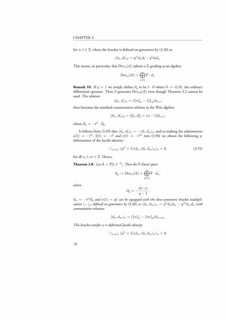
CHAPTER 3.

for n, l ∈ Z, where the bracket is defined on generators by (3.20) as

〈dn, dl〉σ = qndndl − qldldn.

This means, in particular, that Derσ(A) admits a Z-grading as an algebra:

Derσ(A) =⊕i∈Z

F · di.

Remark 10. If q = 1 we simply define ∂q to be t · ∂ where ∂ := d/dt, the ordinarydifferential operator. Then ∂ generates Derid(A) even though Theorem 3.2 cannot beused. The relation

〈dn, dl〉σ = (nq − lq)dn+l

then becomes the standard commutation relation in the Witt algebra:

〈∂n, ∂l〉id = [∂n, ∂l] = (n− l)∂n+l,

where ∂n = −tn · ∂q.

It follows from (3.49) that 〈dn, dl〉σ = −〈dl, dn〉σ , and so making the substitutionsa(t) = −tn, b(t) = −tl and c(t) = −tm into (3.50) we obtain the following q-deformation of the Jacobi identity:

n,m,l (qn + 1)〈dn, 〈dl, dm〉σ〉σ = 0, (3.55)

for all n, l,m ∈ Z. Hence,

Theorem 3.8. Let A = F[t, t−1]. Then the F-linear space

dq := Derσ(A) =⊕n∈Z

F · dn,

where

∂q = − id−σq − 1

,

dn = −tn∂q and σ(t) = qt can be equipped with the skew-symmetric bracket multipli-cation 〈·, ·〉σ defined on generators by (3.20) as 〈dn, dm〉σ = qndndm − qmdmdn withcommutation relations

〈dn, dm〉σ = (nq − mq)dn+m.

This bracket satisfies a σ-deformed Jacobi identity

n,m,l (qn + 1)〈dn, 〈dl, dm〉σ〉σ = 0.

70

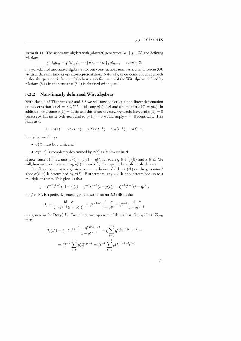
3.3. EXAMPLES

Remark 11. The associative algebra with (abstract) generators dj | j ∈ Z and definingrelations

qndndm − qmdmdn = (nq − mq)dn+m, n,m ∈ Zis a well-defined associative algebra, since our construction, summarized in Theorem 3.8,yields at the same time its operator representation. Naturally, an outcome of our approachis that this parametric family of algebras is a deformation of the Witt algebra defined byrelations (3.1) in the sense that (3.1) is obtained when q = 1.

3.3.2 Non-linearly deformed Witt algebras

With the aid of Theorems 3.2 and 3.3 we will now construct a non-linear deformationof the derivations of A = F[t, t−1]. Take any p(t) ∈ A and assume that σ(t) = p(t). Inaddition, we assume σ(1) = 1, since if this is not the case, we would have had σ(1) = 0because A has no zero-divisors and so σ(1) = 0 would imply σ = 0 identically. Thisleads us to

1 = σ(1) = σ(t · t−1) = σ(t)σ(t−1) =⇒ σ(t−1) = σ(t)−1,

implying two things:

• σ(t) must be a unit, and

• σ(t−1) is completely determined by σ(t) as its inverse in A.

Hence, since σ(t) is a unit, σ(t) = p(t) = qts, for some q ∈ F \ 0 and s ∈ Z. Wewill, however, continue writing p(t) instead of qts except in the explicit calculations.

It suffices to compute a greatest common divisor of (id−σ)(A) on the generator tsince σ(t−1) is determined by σ(t). Furthermore, any gcd is only determined up to amultiple of a unit. This gives us that

g = ζ−1tk−1(id−σ)(t) = ζ−1tk−1(t− p(t)) = ζ−1tk−1(t− qts),

for ζ ∈ F∗, is a perfectly general gcd and so Theorem 3.2 tells us that

∂σ =id−σ

ζ−1tk−1(t− p(t))= ζt−k+1 id−σ

t− qts= ζt−k id−σ

1− qts−1

is a generator for Derσ(A). Two direct consequences of this is that, firstly, if r ∈ Z≥0,then

∂σ(tr) = ζ · t−k+r 1− qrtr(s−1)

1− qts−1= ζ

r−1∑l=0

qlt(s−1)l+r−k =

= ζt−kr−1∑l=0

p(t)ltr−l = ζt−kr−1∑l=0

p(t)r−1−ltl+1

71

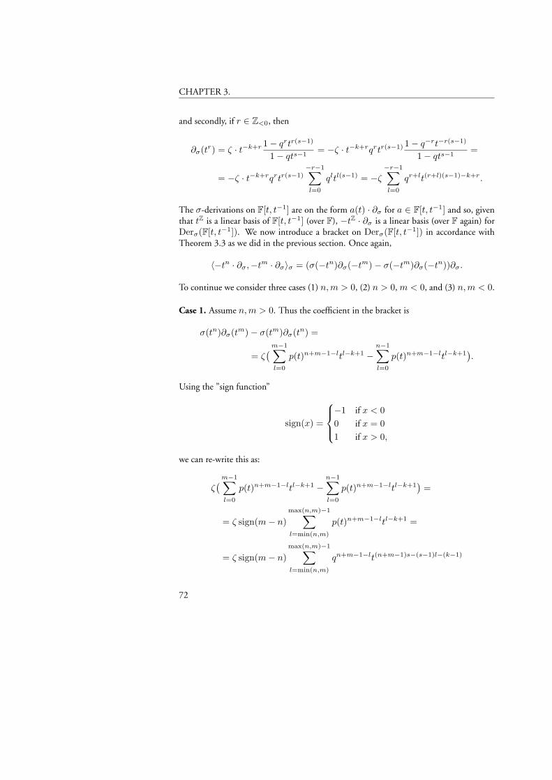
CHAPTER 3.

and secondly, if r ∈ Z<0, then

∂σ(tr) = ζ · t−k+r 1− qrtr(s−1)

1− qts−1= −ζ · t−k+rqrtr(s−1) 1− q−rt−r(s−1)

1− qts−1=

= −ζ · t−k+rqrtr(s−1)−r−1∑l=0

qltl(s−1) = −ζ−r−1∑l=0

qr+lt(r+l)(s−1)−k+r.

The σ-derivations on F[t, t−1] are on the form a(t) · ∂σ for a ∈ F[t, t−1] and so, giventhat tZ is a linear basis of F[t, t−1] (over F), −tZ · ∂σ is a linear basis (over F again) forDerσ(F[t, t−1]). We now introduce a bracket on Derσ(F[t, t−1]) in accordance withTheorem 3.3 as we did in the previous section. Once again,

〈−tn · ∂σ,−tm · ∂σ〉σ = (σ(−tn)∂σ(−tm)− σ(−tm)∂σ(−tn))∂σ.

To continue we consider three cases (1) n,m > 0, (2) n > 0, m < 0, and (3) n,m < 0.

Case 1. Assume n,m > 0. Thus the coefficient in the bracket is

σ(tn)∂σ(tm)− σ(tm)∂σ(tn) =

= ζ( m−1∑

l=0

p(t)n+m−1−ltl−k+1 −n−1∑l=0

p(t)n+m−1−ltl−k+1).

Using the ”sign function”

sign(x) =

−1 if x < 00 if x = 01 if x > 0,

we can re-write this as:

ζ( m−1∑

l=0

p(t)n+m−1−ltl−k+1 −n−1∑l=0

p(t)n+m−1−ltl−k+1)

=

= ζ sign(m− n)max(n,m)−1∑l=min(n,m)

p(t)n+m−1−ltl−k+1 =

= ζ sign(m− n)max(n,m)−1∑l=min(n,m)

qn+m−1−lt(n+m−1)s−(s−1)l−(k−1)

72

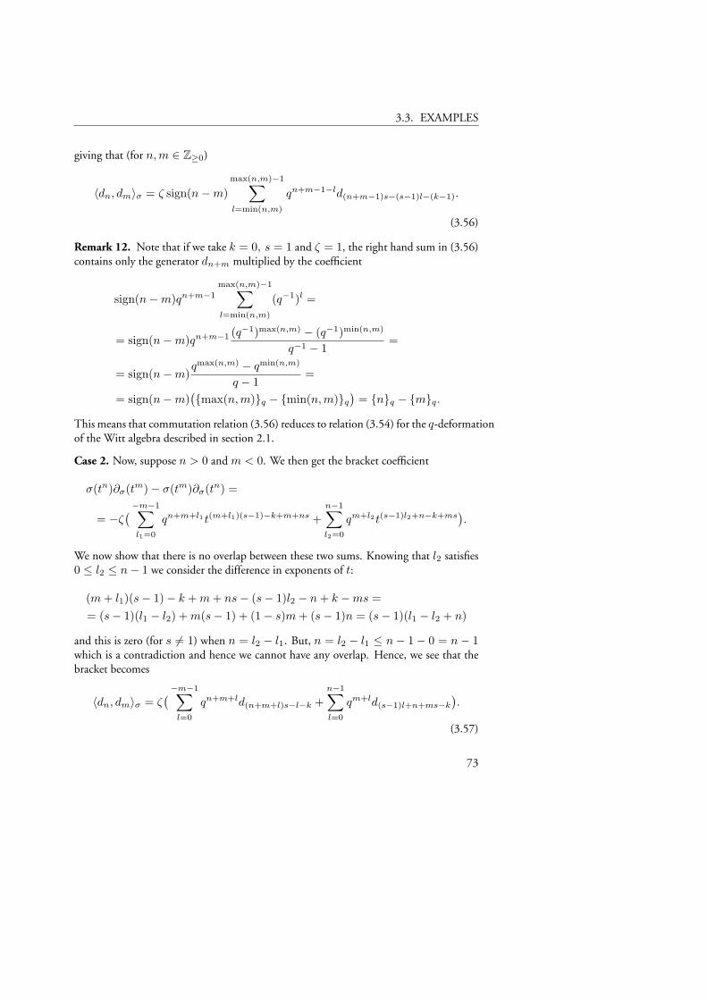
3.3. EXAMPLES

giving that (for n,m ∈ Z≥0)

〈dn, dm〉σ = ζ sign(n−m)max(n,m)−1∑l=min(n,m)

qn+m−1−ld(n+m−1)s−(s−1)l−(k−1).

(3.56)

Remark 12. Note that if we take k = 0, s = 1 and ζ = 1, the right hand sum in (3.56)contains only the generator dn+m multiplied by the coefficient

sign(n−m)qn+m−1

max(n,m)−1∑l=min(n,m)

(q−1)l =

= sign(n−m)qn+m−1 (q−1)max(n,m) − (q−1)min(n,m)

q−1 − 1=

= sign(n−m)qmax(n,m) − qmin(n,m)

q − 1=

= sign(n−m)(max(n,m)q − min(n,m)q

)= nq − mq.

This means that commutation relation (3.56) reduces to relation (3.54) for the q-deformationof the Witt algebra described in section 2.1.

Case 2. Now, suppose n > 0 and m < 0. We then get the bracket coefficient

σ(tn)∂σ(tm)− σ(tm)∂σ(tn) =

= −ζ(−m−1∑

l1=0

qn+m+l1t(m+l1)(s−1)−k+m+ns +n−1∑l2=0

qm+l2t(s−1)l2+n−k+ms).

We now show that there is no overlap between these two sums. Knowing that l2 satisfies0 ≤ l2 ≤ n− 1 we consider the difference in exponents of t:

(m+ l1)(s− 1)− k +m+ ns− (s− 1)l2 − n+ k −ms == (s− 1)(l1 − l2) +m(s− 1) + (1− s)m+ (s− 1)n = (s− 1)(l1 − l2 + n)

and this is zero (for s 6= 1) when n = l2 − l1. But, n = l2 − l1 ≤ n− 1− 0 = n− 1which is a contradiction and hence we cannot have any overlap. Hence, we see that thebracket becomes

〈dn, dm〉σ = ζ(−m−1∑

l=0

qn+m+ld(n+m+l)s−l−k +n−1∑l=0

qm+ld(s−1)l+n+ms−k

).

(3.57)

73

CHAPTER 3.

Case 2′. By interchanging the role of n and m so that m > 0 and n < 0 we get instead

σ(tn)∂σ(tm)− σ(tm)∂σ(tn) =

= ζ( m−1∑

l1=0

qn+l1t(s−1)l1+m+ns−k +−n−1∑l2=0

qm+n+l2t(n+l2)(s−1)+n+ms−k),

so the coefficient for the bracket becomes

〈dn, dm〉σ = −ζ( m−1∑

l=0

qn+ld(s−1)l+m+ns−k +−n−1∑l=0

qm+n+ld(n+m+l)s−l−k

).

(3.58)

Remark 13. If we put k = 0, s = 1 and ζ = 1 in Case 2 and 2′, we once again get thesingle generator dn+m multiplied with

qn+m−m−1∑

l=0

ql + qmn−1∑l=0

ql = qm+n 1− q−m

1− q+ qm 1− qn

1− q=

= −qn 1− qm

1− q+ qm 1− qn

1− q=qm − qn

1− q=

= nq − mq,

just as we would expect from the case in the previous section.

Case 3. Both n,m < 0. This leads to

σ(tn)∂σ(tm)− σ(tm)∂σ(tn) =

= −ζ(−m−1∑

l1=0

qn+m+l1t(m+n)s+(s−1)l1−k −−n−1∑l2=0

qn+m+l2t(n+m)s+(s−1)l2−k).

Hence we have a bracket coefficient resembling that of Case 1, namely

〈dn, dm〉σ = ζ sign(n−m)max(−n,−m)−1∑l=min(−n,−m)

qn+m+ld(m+n)s+(s−1)l−k. (3.59)

We can now, from (3.31), calculate δ to get

δ =σ(g)g

=ζ−1tsk(1− qsts(s−1))ζ−1tk(1− qts−1)

= qktk(s−1)s−1∑r=0

(qts−1)r.

74

3.3. EXAMPLES

By the definition of δ, ∂σ and σ span a ”quantum plane”-like commutation relation

∂σσ = qktk(s−1)s−1∑r=0

(qts−1)r · σ∂σ.

To get a hom-Lie algebra it is enough for δ to belong to F and this can be achieved onlywhen s = 1, that is, when the deformation is linear (i.e., when σ homogeneous of degreezero).

Theorem 3.3 now tells us what a generalized Jacobi identity looks like

n,m,l

(qn〈dns, 〈dm, dl〉σ〉σ + qktk(s−1)

s−1∑r=0

(qts−1)r〈dn, 〈dm, dl〉σ〉σ)

= 0.

The hom-Lie algebra Jacobi-identity (s = 1) becomes

n,m,l (qn + qk)〈dn, 〈dm, dl〉σ〉σ = 0.

We summarize these findings in a theorem.

Theorem 3.9. Let A = F[t, t−1]. Then the F-linear space

Derσ(A) =⊕n∈Z

F · dn,

where

∂σ = ζt−k+1 id−σt− qts

,

dn = −tn∂σ and σ(t) = qts, can be equipped with the skew-symmetric bracket product〈 ·, ·〉σ defined on generators by (3.20) as 〈dn, dm〉σ = qndnsdm−qmdmsdn and satisfyingdefining commutation relations

〈dn, dm〉σ = ζ sign(n−m)max(n,m)−1∑l=min(n,m)

qn+m−1−lds(n+m−1)−(k−1)−l(s−1)

for n,m ≥ 0;

〈dn, dm〉σ = ζ(−m−1∑

l=0

qn+m+ld(n+m+l)s−l−k +n−1∑l=0

qm+ld(s−1)l+n+ms−k

)for n ≥ 0,m < 0;

75

CHAPTER 3.

〈dn, dm〉σ = −ζ( m−1∑

l=0

qn+ld(s−1)l1+m+ns−k +−n−1∑l=0

qm+n+ld(n+m+l)s−l−k

)for m ≥ 0, n < 0;

〈dn, dm〉σ = ζ sign(n−m)max(−n,−m)−1∑l=min(−n,−m)

qn+m+ld(m+n)s+(s−1)l−k

for n,m < 0.

Furthermore, we have a σ-deformed Jacobi identity

n,m,l

(qn〈dns, 〈dm, dl〉σ〉σ + qktk(s−1)

s−1∑r=0

(qts−1)r〈dn, 〈dm, dl〉σ〉σ)

= 0.

Remark 14. Note that by performing a change of basis and consider instead dn =−tn+k∂σ in the definition of dn we can evade the use of k altogether. Hence we see thatthe k-shifted grading is something resulting from a choice of basis for M.

Remark 15. The associative algebra with an infinite number of (abstract) generatorsdj | j ∈ Z and defining relations

qndnsdm − qmdmsdn =

Eq. (3.56) for n,m ≥ 0Eq. (3.57) for n ≥ 0,m < 0Eq. (3.58) for m ≥ 0, n < 0Eq. (3.59) for n,m < 0

is a well-defined associative algebra, since our construction yields at the same time itsoperator representation. Naturally, an outcome of our approach is that this parametricfamily of algebras is a deformation of the Witt algebra defined by relations (3.1) in thesense that (3.1) is obtained when q = 1 and k = 0, s = 1, ζ = 1.

A submodule of Derσ(F[t, t−1])

We let, as before, A = F[t, t−1], the algebra of Laurent polynomials, and σ be somenon-zero endomorphism such that σ(t) = p(t). In the previous section we showed thatany greatest common divisor of (id−σ)(A) has the form

ζ−1tk−1(t− p(t)) = ζ−1tk(1− qts−1)

for k ∈ Z and nonzero ζ ∈ F. As described in Remark 5, this means that

∂σ =id−σζ−1 · tk

76

3.3. EXAMPLES

generates a proper cyclic A-submodule M of Derσ(A), unless we have p(t) = ηt forsome η ∈ F∗.

As above we calculate δ using (3.31) and we find

δ = qkt(s−1)k

which means that ∂σ and σ satisfy the following relation

∂σσ = qkt(s−1)kσ∂σ.

We set dn = −tn∂σ. Before we calculate the bracket, we note that

∂σ(t) = ζt−k+1(1− qts−1),

andζ(id−σ)t−k

(tr

)= ζtr−k(1− qrt(s−1)r).

The coefficient of ∂σ in the bracket 〈dn, dm〉σ then becomes

σ(tn)∂σ(tm)− σ(tm)∂σ(tn) = ζqntns+m−k − ζqmtms+n−k

which means that

〈dn, dm〉σ = ζqmdms+n−k − ζqndns+m−k,

where〈dn, dm〉σ = qndnsdm − qmdmsdn

by (3.20). Putting a = −tn, b = −tm and c = −tl in (3.23) with δ = qkt(s−1)k we get

n,m,l

(〈−qntns∂σ, 〈−tm∂σ,−tl∂σ〉σ〉σ+

+ qkt(s−1)k〈−tn∂σ, 〈−tm∂σ,−tl∂σ〉σ〉σ)

=

=n,m,l

(qn〈dns, 〈dm, dl〉σ〉σ + qkt(s−1)k〈dn, 〈dm, dl〉σ〉σ

)= 0.

Theorem 3.10. The F-linear space

M =⊕i∈Z

F · di with di = −ti∂σ

of σ-derivations on A allows a structure as an algebra with skew-symmetric bracket defined ongenerators (by (3.20) again) as 〈dn, dm〉σ = qndnsdm− qmdmsdn and satisfying relations

〈dn, dm〉σ = ζqmdms+n−k − ζqndns+m−k,

with s ∈ Z and ζ ∈ F. The σ-deformed Jacobi identity becomes

n,m,l

(qn〈dns, 〈dm, dl〉σ〉σ + qkt(s−1)k〈dn, 〈dm, dl〉σ〉σ

)= 0.

77

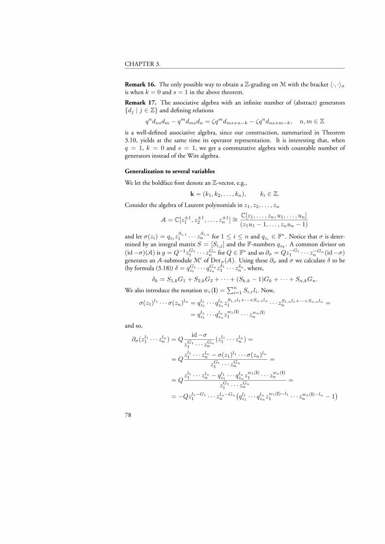
CHAPTER 3.

Remark 16. The only possible way to obtain a Z-grading on M with the bracket 〈·, ·〉σis when k = 0 and s = 1 in the above theorem.

Remark 17. The associative algebra with an infinite number of (abstract) generatorsdj | j ∈ Z and defining relations

qndnsdm − qmdmsdn = ζqmdms+n−k − ζqndns+m−k, n,m ∈ Z

is a well-defined associative algebra, since our construction, summarized in Theorem3.10, yields at the same time its operator representation. It is interesting that, whenq = 1, k = 0 and s = 1, we get a commutative algebra with countable number ofgenerators instead of the Witt algebra.

Generalization to several variables

We let the boldface font denote an Z-vector, e.g.,

k = (k1, k2, . . . , kn), ki ∈ Z.

Consider the algebra of Laurent polynomials in z1, z2, . . . , zn

A = C[z±11 , z±1

2 , . . . , z±1n ] ∼=

C[z1, . . . , zn, u1, . . . , un](z1u1 − 1, . . . , znun − 1)

and let σ(zi) = qziz

Si,11 · · · zSi,n

n for 1 ≤ i ≤ n and qzi∈ F∗. Notice that σ is deter-

mined by an integral matrix S = [Si,j ] and the F-numbers qzk. A common divisor on

(id−σ)(A) is g = Q−1zG11 · · · zGn

n for Q ∈ F∗ and so ∂σ = Qz−G11 · · · z−Gn

n (id−σ)generates an A-submodule M′ of Derσ(A). Using these ∂σ and σ we calculate δ to be(by formula (3.18)) δ = qG1

z1· · · qGn

znzδ11 · · · zδn

n , where,

δk = S1,kG1 + S2,kG2 + · · ·+ (Sk,k − 1)Gk + · · ·+ Sn,kGn.

We also introduce the notation wr(l) =∑n

i=1 Si,rli. Now,

σ(z1)l1 · · ·σ(zn)ln = ql1z1· · · qln

znz

S1,1l1+···+Sn,1ln1 · · · zS1,nl1+···+Sn,nln

n =

= ql1z1· · · qln

znz

w1(l)1 · · · zwn(l)

n

and so,

∂σ(zl11 · · · zln

n ) = Qid−σ

zG11 · · · zGn

n

(zl11 · · · zln

n ) =

= Qzl11 · · · zln

n − σ(z1)l1 · · ·σ(zn)ln

zG11 · · · zGn

n

=

= Qzl11 · · · zln

n − ql1z1· · · qln

znz

w1(l)1 · · · zwn(l)

n

zG11 · · · zGn

n

=

= −Qzl1−G11 · · · zln−Gn

n

(ql1z1· · · qln

znz

w1(l)−l11 · · · zwn(l)−ln

n − 1)

78

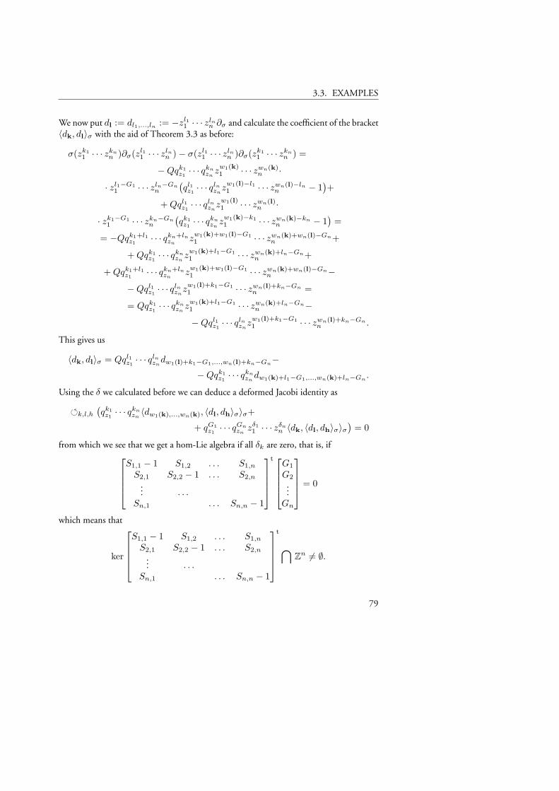
3.3. EXAMPLES

We now put dl := dl1,...,ln := −zl11 · · · zln

n ∂σ and calculate the coefficient of the bracket〈dk, dl〉σ with the aid of Theorem 3.3 as before:

σ(zk11 · · · zkn

n )∂σ(zl11 · · · zln

n )− σ(zl11 · · · zln

n )∂σ(zk11 · · · zkn

n ) =

−Qqk1z1· · · qkn

znz

w1(k)1 · · · zwn(k)

n ·

· zl1−G11 · · · zln−Gn

n

(ql1z1· · · qln

znz

w1(l)−l11 · · · zwn(l)−ln

n − 1)+

+Qql1z1· · · qln

znz

w1(l)1 · · · zwn(l)

n ·

· zk1−G11 · · · zkn−Gn

n

(qk1z1· · · qkn

znz

w1(k)−k11 · · · zwn(k)−kn

n − 1)

=

= −Qqk1+l1z1

· · · qkn+lnzn

zw1(k)+w1(l)−G11 · · · zwn(k)+wn(l)−Gn

n +

+Qqk1z1· · · qkn

znz

w1(k)+l1−G11 · · · zwn(k)+ln−Gn

n +

+Qqk1+l1z1

· · · qkn+lnzn

zw1(k)+w1(l)−G11 · · · zwn(k)+wn(l)−Gn

n −

−Qql1z1· · · qln

znz

w1(l)+k1−G11 · · · zwn(l)+kn−Gn

n =

= Qqk1z1· · · qkn

znz

w1(k)+l1−G11 · · · zwn(k)+ln−Gn

n −

−Qql1z1· · · qln

znz

w1(l)+k1−G11 · · · zwn(l)+kn−Gn

n .

This gives us

〈dk, dl〉σ = Qql1z1· · · qln

zndw1(l)+k1−G1,...,wn(l)+kn−Gn

−−Qqk1

z1· · · qkn

zndw1(k)+l1−G1,...,wn(k)+ln−Gn

.

Using the δ we calculated before we can deduce a deformed Jacobi identity as

k,l,h

(qk1z1· · · qkn

zn〈dw1(k),...,wn(k), 〈dl, dh〉σ〉σ+

+ qG1z1· · · qGn

znzδ11 · · · zδn

n 〈dk, 〈dl, dh〉σ〉σ)

= 0

from which we see that we get a hom-Lie algebra if all δk are zero, that is, ifS1,1 − 1 S1,2 . . . S1,n

S2,1 S2,2 − 1 . . . S2,n

... . . .Sn,1 . . . Sn,n − 1

t G1

G2

...Gn

= 0

which means that

ker

S1,1 − 1 S1,2 . . . S1,n

S2,1 S2,2 − 1 . . . S2,n

... . . .Sn,1 . . . Sn,n − 1

t ⋂

Zn 6= ∅.

79

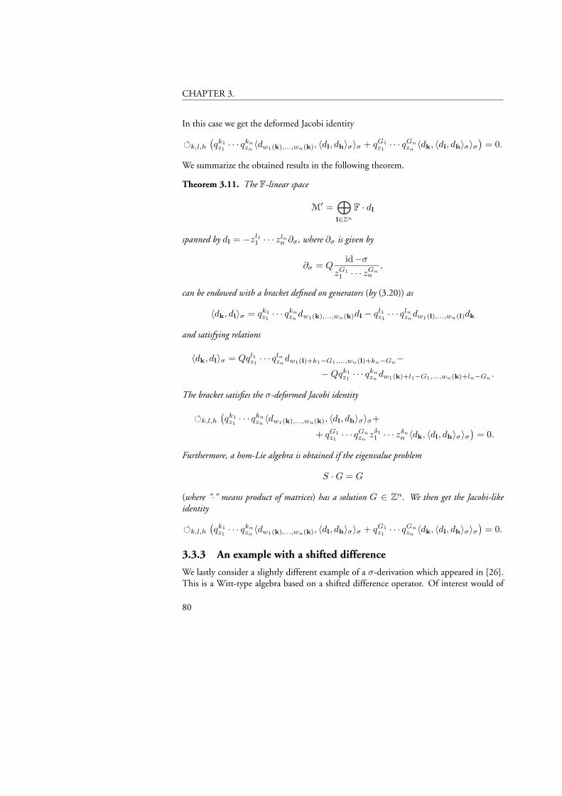
CHAPTER 3.

In this case we get the deformed Jacobi identity

k,l,h

(qk1z1· · · qkn

zn〈dw1(k),...,wn(k), 〈dl, dh〉σ〉σ + qG1

z1· · · qGn

zn〈dk, 〈dl, dh〉σ〉σ

)= 0.

We summarize the obtained results in the following theorem.

Theorem 3.11. The F-linear space

M′ =⊕l∈Zn

F · dl

spanned by dl = −zl11 · · · zln

n ∂σ , where ∂σ is given by

∂σ = Qid−σ

zG11 · · · zGn

n

,

can be endowed with a bracket defined on generators (by (3.20)) as

〈dk, dl〉σ = qk1z1· · · qkn

zndw1(k),...,wn(k)dl − ql1

z1· · · qln

zndw1(l),...,wn(l)dk

and satisfying relations

〈dk, dl〉σ = Qql1z1· · · qln

zndw1(l)+k1−G1,...,wn(l)+kn−Gn

−−Qqk1

z1· · · qkn

zndw1(k)+l1−G1,...,wn(k)+ln−Gn

.

The bracket satisfies the σ-deformed Jacobi identity

k,l,h

(qk1z1· · · qkn

zn〈dw1(k),...,wn(k), 〈dl, dh〉σ〉σ+

+ qG1z1· · · qGn

znzδ11 · · · zδn

n 〈dk, 〈dl, dh〉σ〉σ)

= 0.

Furthermore, a hom-Lie algebra is obtained if the eigenvalue problem

S ·G = G

(where ”·” means product of matrices) has a solution G ∈ Zn. We then get the Jacobi-likeidentity

k,l,h

(qk1z1· · · qkn

zn〈dw1(k),...,wn(k), 〈dl, dh〉σ〉σ + qG1

z1· · · qGn

zn〈dk, 〈dl, dh〉σ〉σ

)= 0.

3.3.3 An example with a shifted difference

We lastly consider a slightly different example of a σ-derivation which appeared in [26].This is a Witt-type algebra based on a shifted difference operator. Of interest would of

80

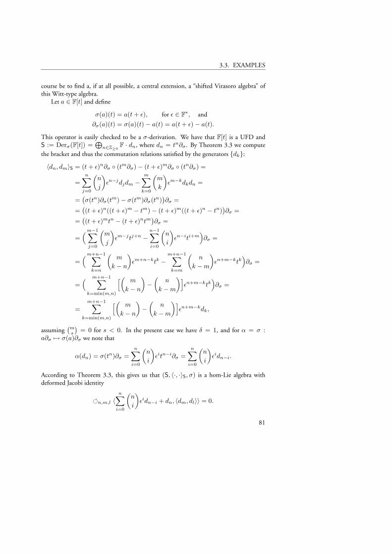
3.3. EXAMPLES

course be to find a, if at all possible, a central extension, a “shifted Virasoro algebra” ofthis Witt-type algebra.

Let a ∈ F[t] and define

σ(a)(t) = a(t+ ε), for ε ∈ F∗, and

∂σ(a)(t) = σ(a)(t)− a(t) = a(t+ ε)− a(t).

This operator is easily checked to be a σ-derivation. We have that F[t] is a UFD andS := Derσ(F[t]) =

⊕n∈Z≥0

F · dn, where dn = tn∂σ . By Theorem 3.3 we computethe bracket and thus the commutation relations satisfied by the generators dk:

〈dn, dm〉S = (t+ ε)n∂σ (tm∂σ)− (t+ ε)m∂σ (tn∂σ) =

=n∑

j=0

(n

j

)εn−jdjdm −

m∑k=0

(m

k

)εm−kdkdn =

=(σ(tn)∂σ(tm)− σ(tm)∂σ(tn)

)∂σ =

=((t+ ε)n((t+ ε)m − tm)− (t+ ε)m((t+ ε)n − tn)

)∂σ =

=((t+ ε)mtn − (t+ ε)ntm

)∂σ =

=( m−1∑

j=0

(m

j

)εm−jtj+n −

n−1∑i=0

(n

i

)εn−iti+m

)∂σ =

=( m+n−1∑

k=n

(m

k − n

)εm+n−ktk −

m+n−1∑k=m

(n

k −m

)εn+m−ktk

)∂σ =

=( m+n−1∑

k=min(m,n)

[( m

k − n

)−

(n

k −m

)]εn+m−ktk

)∂σ =

=m+n−1∑

k=min(m,n)

[( m

k − n

)−

(n

k −m

)]εn+m−kdk,

assuming(ms

)= 0 for s < 0. In the present case we have δ = 1, and for α = σ :

a∂σ 7→ σ(a)∂σ we note that

α(dn) = σ(tn)∂σ =n∑

i=0

(n

i

)εitn−i∂σ =

n∑i=0

(n

i

)εidn−i.

According to Theorem 3.3, this gives us that (S, 〈·, ·〉S, σ) is a hom-Lie algebra withdeformed Jacobi identity

n,m,l 〈n∑

i=0

(n

i

)εidn−i + dn, 〈dm, dl〉〉 = 0.

81

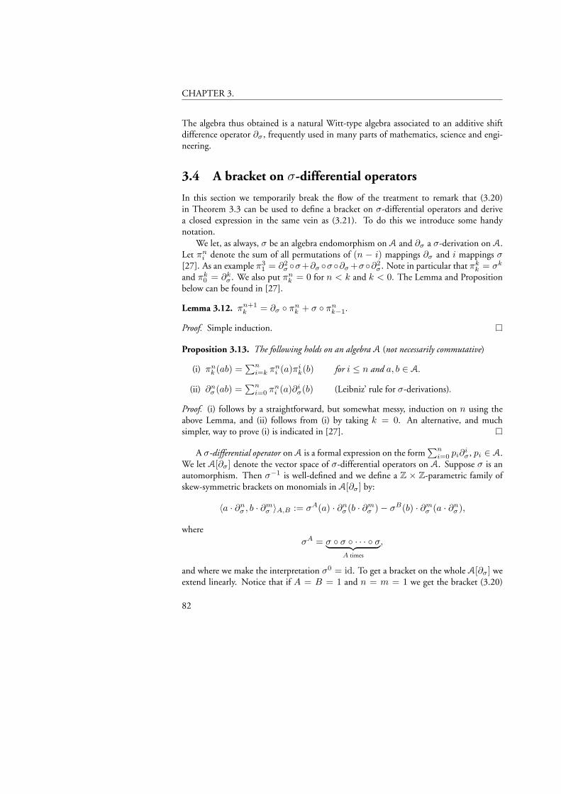
CHAPTER 3.

The algebra thus obtained is a natural Witt-type algebra associated to an additive shiftdifference operator ∂σ , frequently used in many parts of mathematics, science and engi-neering.

3.4 A bracket on σ-differential operators

In this section we temporarily break the flow of the treatment to remark that (3.20)in Theorem 3.3 can be used to define a bracket on σ-differential operators and derivea closed expression in the same vein as (3.21). To do this we introduce some handynotation.

We let, as always, σ be an algebra endomorphism on A and ∂σ a σ-derivation on A.Let πn

i denote the sum of all permutations of (n − i) mappings ∂σ and i mappings σ[27]. As an example π3

1 = ∂2σ σ+∂σ σ∂σ +σ∂2

σ . Note in particular that πkk = σk

and πk0 = ∂k

σ . We also put πnk = 0 for n < k and k < 0. The Lemma and Proposition

below can be found in [27].

Lemma 3.12. πn+1k = ∂σ πn

k + σ πnk−1.

Proof. Simple induction.

Proposition 3.13. The following holds on an algebra A (not necessarily commutative)

(i) πnk (ab) =

∑ni=k π

ni (a)πi

k(b) for i ≤ n and a, b ∈ A.

(ii) ∂nσ (ab) =

∑ni=0 π

ni (a)∂i

σ(b) (Leibniz’ rule for σ-derivations).

Proof. (i) follows by a straightforward, but somewhat messy, induction on n using theabove Lemma, and (ii) follows from (i) by taking k = 0. An alternative, and muchsimpler, way to prove (i) is indicated in [27].

A σ-differential operator on A is a formal expression on the form∑n

i=0 pi∂iσ , pi ∈ A.

We let A[∂σ] denote the vector space of σ-differential operators on A. Suppose σ is anautomorphism. Then σ−1 is well-defined and we define a Z × Z-parametric family ofskew-symmetric brackets on monomials in A[∂σ] by:

〈a · ∂nσ , b · ∂m

σ 〉A,B := σA(a) · ∂nσ (b · ∂m

σ )− σB(b) · ∂mσ (a · ∂n

σ ),

whereσA = σ σ · · · σ︸ ︷︷ ︸

A times

,

and where we make the interpretation σ0 = id. To get a bracket on the whole A[∂σ] weextend linearly. Notice that if A = B = 1 and n = m = 1 we get the bracket (3.20)

82

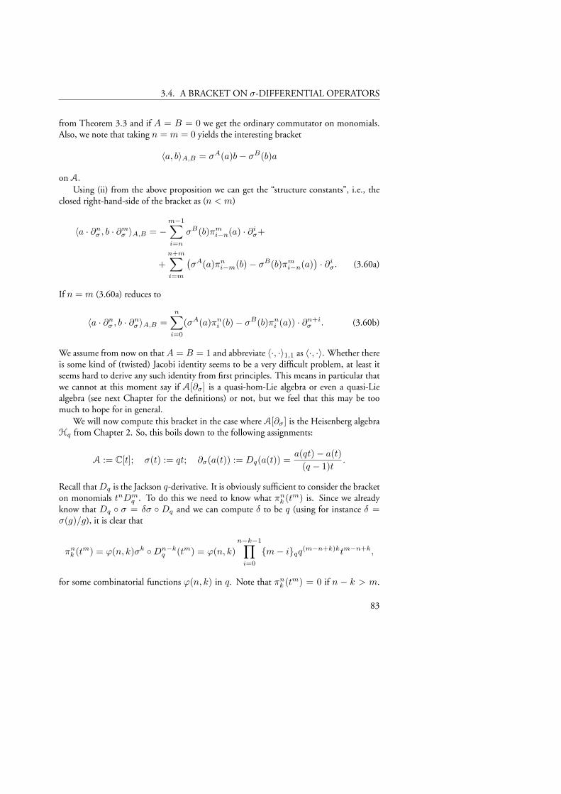
3.4. A BRACKET ON σ-DIFFERENTIAL OPERATORS

from Theorem 3.3 and if A = B = 0 we get the ordinary commutator on monomials.Also, we note that taking n = m = 0 yields the interesting bracket

〈a, b〉A,B = σA(a)b− σB(b)a

on A.Using (ii) from the above proposition we can get the “structure constants”, i.e., the

closed right-hand-side of the bracket as (n < m)

〈a · ∂nσ , b · ∂m

σ 〉A,B = −m−1∑i=n

σB(b)πmi−n(a) · ∂i

σ+

+n+m∑i=m

(σA(a)πn

i−m(b)− σB(b)πmi−n(a)

)· ∂i

σ. (3.60a)

If n = m (3.60a) reduces to

〈a · ∂nσ , b · ∂n

σ 〉A,B =n∑

i=0

(σA(a)πni (b)− σB(b)πn

i (a)) · ∂n+iσ . (3.60b)

We assume from now on thatA = B = 1 and abbreviate 〈·, ·〉1,1 as 〈·, ·〉. Whether thereis some kind of (twisted) Jacobi identity seems to be a very difficult problem, at least itseems hard to derive any such identity from first principles. This means in particular thatwe cannot at this moment say if A[∂σ] is a quasi-hom-Lie algebra or even a quasi-Liealgebra (see next Chapter for the definitions) or not, but we feel that this may be toomuch to hope for in general.

We will now compute this bracket in the case where A[∂σ] is the Heisenberg algebraHq from Chapter 2. So, this boils down to the following assignments:

A := C[t]; σ(t) := qt; ∂σ(a(t)) := Dq(a(t)) =a(qt)− a(t)

(q − 1)t.

Recall thatDq is the Jackson q-derivative. It is obviously sufficient to consider the bracketon monomials tnDm

q . To do this we need to know what πnk (tm) is. Since we already

know that Dq σ = δσ Dq and we can compute δ to be q (using for instance δ =σ(g)/g), it is clear that

πnk (tm) = ϕ(n, k)σk Dn−k

q (tm) = ϕ(n, k)n−k−1∏

i=0

m− iqq(m−n+k)ktm−n+k,

for some combinatorial functions ϕ(n, k) in q. Note that πnk (tm) = 0 if n − k > m.

83

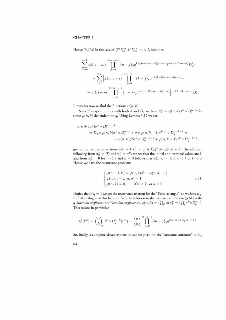
CHAPTER 3.

Hence (3.60a) in the case of 〈tnDmq , t

kDlq〉, m < l, becomes:

−l−1∑i=m

ϕ(l, i−m)l+m−i−1∏

j=0

n− jqqk+(n−(l+m−i))(i−m)tn+k−(l+m−i)Di

q+

+m+l∑i=l

[ϕ(m, i− l)

l+m−i−1∏j=0

k − jqqn+(k−(l+m−i))(i−l)−

− ϕ(l, i−m)l+m−i−1∏

j=0

n− jqqk+(n−(l+m−i))(i−m)

]tn+k−(l+m−i)Di

q.

It remains now to find the functions ϕ(n, k).Since δ = q commutes with both σ and Dq we have πn

k = ϕ(n, k)σk Dn−kq for

some ϕ(n, k) dependent on q. Using Lemma 3.12 we see

ϕ(n+ 1, k)σk Dn+1−kq =

= Dq ϕ(n, k)σk Dn−kq + σ ϕ(n, k − 1)σk−1 Dn−k+1

q =

= ϕ(n, k)qkσk Dn−k+1q + ϕ(n, k − 1)σk Dn−k+1

q ,

giving the recurrence relation ϕ(n + 1, k) = ϕ(n, k)qk + ϕ(n, k − 1). In addition,following from πn

0 = ∂nσ and πn

n = σn, we see that the initial and terminal values are 1,and from πn

k = 0 for n < k and k < 0 follows that ϕ(n, k) = 0 if n < k or k < 0.Hence we have the recurrence problem:

ϕ(n+ 1, k) = ϕ(n, k)qk + ϕ(n, k − 1),ϕ(n, 0) = ϕ(n, n) = 1,ϕ(n, k) = 0, if n < k, or k < 0.

(3.61)

Notice that if q = 1 we get the recurrence relation for the “Pascal triangle”, so we have a q-shifted analogue of this here. In fact, the solution to the recurrence problem (3.61) is theq-binomial coefficients (or Gaussian coefficients), ϕ(n, k) =

(nk

)q, so πn

k =(nk

)qσkDn−k

q .

This means in particular

πnk (tm) =

(n

k

)q

σk Dn−kq (tm) =

(n

k

)q

n−k−1∏j=0

m− jqq(m−n+k)ktm−n+k.

So, finally, a complete closed expression can be given for the “structure constants” of Hq

84

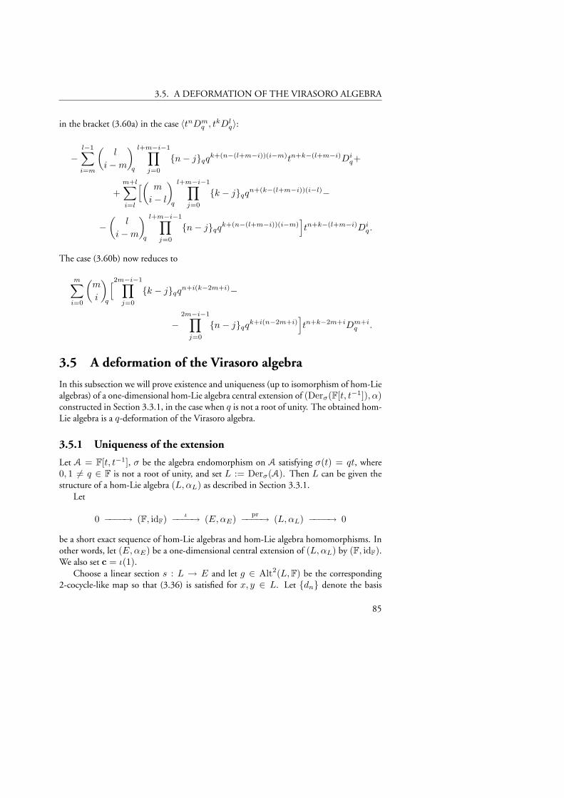
3.5. A DEFORMATION OF THE VIRASORO ALGEBRA

in the bracket (3.60a) in the case 〈tnDmq , t

kDlq〉:

−l−1∑i=m

(l

i−m

)q

l+m−i−1∏j=0

n− jqqk+(n−(l+m−i))(i−m)tn+k−(l+m−i)Di

q+

+m+l∑i=l

[( m

i− l

)q

l+m−i−1∏j=0

k − jqqn+(k−(l+m−i))(i−l)−

−(

l

i−m

)q

l+m−i−1∏j=0

n− jqqk+(n−(l+m−i))(i−m)

]tn+k−(l+m−i)Di

q.

The case (3.60b) now reduces to

m∑i=0

(m

i

)q

[2m−i−1∏j=0

k − jqqn+i(k−2m+i)−

−2m−i−1∏

j=0

n− jqqk+i(n−2m+i)

]tn+k−2m+iDm+i

q .

3.5 A deformation of the Virasoro algebra

In this subsection we will prove existence and uniqueness (up to isomorphism of hom-Liealgebras) of a one-dimensional hom-Lie algebra central extension of (Derσ(F[t, t−1]), α)constructed in Section 3.3.1, in the case when q is not a root of unity. The obtained hom-Lie algebra is a q-deformation of the Virasoro algebra.

3.5.1 Uniqueness of the extension

Let A = F[t, t−1], σ be the algebra endomorphism on A satisfying σ(t) = qt, where0, 1 6= q ∈ F is not a root of unity, and set L := Derσ(A). Then L can be given thestructure of a hom-Lie algebra (L,αL) as described in Section 3.3.1.

Let

0 −−−−→ (F, idF) ι−−−−→ (E,αE)pr−−−−→ (L,αL) −−−−→ 0

be a short exact sequence of hom-Lie algebras and hom-Lie algebra homomorphisms. Inother words, let (E,αE) be a one-dimensional central extension of (L,αL) by (F, idF).We also set c = ι(1).

Choose a linear section s : L → E and let g ∈ Alt2(L,F) be the corresponding2-cocycle-like map so that (3.36) is satisfied for x, y ∈ L. Let dn denote the basis

85

CHAPTER 3.

(3.51) of L. Define a linear map s′ : L→ E by

s′(dn) =s(dn) if n = 0s(dn)− 1

nqι g(d0, dn)c if n 6= 0.

Then s′ is also a section. Using the calculation (3.38) and the commutation relation(3.54) we get

ι g′(dm, dn) = ι g(dm, dn) + (s− s′)〈dm, dn〉L =

=

ι g(dm, dn) if m+ n = 0ι g(dm, dn) + mq−nq

m+nqι g(d0, dm+n) if m+ n 6= 0.

In particular we have g′(d0, dn) = 0 for any n ∈ Z. According to the calculations inSection 3.2.4, the 2-cocycle-like map g′ must satisfy (3.37) for any x, y, z ∈ L. Thus wehave,

k,l,m g′((id+αL)(dk), 〈dl, dm〉L) = 0

for k, l,m ∈ Z. Substituting the definition (3.52) of αL and using the commutationrelation (3.54) again we get

k,l,m (1 + qk)(lq − mq)A(k, l +m) = 0, (3.62)

where we for simplicity have put A(m,n) = g′(dm, dn) for m,n ∈ Z. Using (3.62)with k = 0 and that A(0, n) = 0 for any n ∈ Z we obtain

(1 + ql)mqA(l,m)− (1 + qm)lqA(m, l) = 0,

or, since A is alternating,

((1 + ql)qm − 1q − 1

+ (1 + qm)ql − 1q − 1

))A(l,m) = 0,

which simplifies to

2ql+m − 1q − 1

A(l,m) = 0.

This shows that A(l,m) = 0 unless l +m = 0. Setting B(m) = A(m,−m) we haveso far

〈s′(dm), s′(dn)〉E = (mq − nq)s′(dm+n) + δm+n,0B(m)c.

Using (3.62) with k = −n− 1, l = n, m = 1 we get

(1 + q−n−1)qn − q

q − 1A(−n− 1, n+ 1) + (1 + qn)

q − q−n−1

q − 1A(n,−n)+

+ (1 + q)q−n−1 − qn

q − 1A(1,−1) = 0,

86

3.5. A DEFORMATION OF THE VIRASORO ALGEBRA

or, after multiplication by qn+1,

q(1 + qn+1)n− 1qB(n+ 1) == (1 + qn)n+ 2qB(n)− (1 + q)2n+ 1qB(1). (3.63)

This is a second order linear recurrence equation in B.

Lemma 3.14. The functions B1, B2 : Z → F defined by

B1(m) =q−m

1 + qmm− 1qmqm+ 1q

B2(m) = q−m2mq

are two linear independent solutions of (3.63).

Proof. Substituting B1 for B in (3.63) the left hand side equals

qn− 1qq−n−1nqn+ 1qn+ 2q,

while the right hand side becomes

n+ 2qq−nn− 1qnqn+ 1q − 0.

These expressions are equal. To prove thatB2 is also a solution requires some calculations:

qn−1q(1+q−n−1)2n+2q−n+2q(1+q−n)2nq+2n+1q(1+q−1)2q =

= (nq − qn−1)(q + q−n)(2nq + q2n + q2n+1)−− (nq + qn(q + 1))(1 + q−n)2nq + (2nq + q2n)(1 + q−1)(1 + q) =

= 2nq

(nq(q + q−n)− qn − q−1 − nq(1 + q−n)−− (q + 1)qn − 1− q + 2 + q + q−1

)+

+ (q + 1)q2n(qnq + q−nnq − qn − q−1 + 1 + q−1

)=

= 2nq

(qn − 1− qn − qn(q + 1)− 1 + 2

)+ q2n q + 1

q − 1(−qn + qn) =

=q2n − 1q − 1

(q + 1)(−qn) + q2n q + 1q − 1

(−qn + qn) =

=q + 1q − 1

(qn − q2n−n) = 0.

It remains to show that B1 and B2 are linear independent. If

λB1 + µB2 = 0,

then evaluation at m = 1 gives µq−1(1 + q) = 0 so µ = 0. Since B1 is nonzero, wemust have λ = 0 also.

87

CHAPTER 3.

Thus we haveB(m) = uB1(m) + vB2(m)

for some u, v ∈ F. In terms of g′ this means that

g′(dm, dn) = δm+n,0(uB1(m) + vB2(m)).

Define now yet another section s′′ : L→ E by

s′′(dm) = s′(dm) + δm,0vc.

Then

ι g′′(dm, dn) = ι g′(dm, dn) + (s′ − s′′)〈dm, dn〉L == δm+n,0(uB1(m) + vB2(m))c− (mq − nq)δm+n,0vc.

= δm+n,0(uB1(m) + vB2(m)− vq−m2mq)c == δm+n,0uB1(m)c,

where we used that mq−−mq = q−m2mq. If u = 0 we have a trivial extension.Otherwise we set c′ = 6uc.

It remains to determine the homomorphism αE . Using equation (3.34) we have forx ∈ E,

αE(x) = s′′ αL pr(x) + ι f(x)

for some linear function f : E → F. To determine f , first use (3.35):

f(c′) = f ι(6u) = idF(6u) = 6u.

HenceαE(c′) = c′.

Next, we use (3.40) in Theorem 3.6 to get

f〈s′′(dm), s′′(dn)〉E = g′′(αL(dm), αL(dn)).

By (3.36) we see that

〈s′′(dm), s′′(dn)〉E = s′′〈dm, dn〉L + ι g′′(dm, dn) == (mq − nq)s′′(dm+n) + ι g′′(dm, dn)

and so

(mq − nq)f s′′(dm+n) + f ι g′′(dm, dn) = qm+ng′′(dm, dn)

which is equivalent to

(mq − nq)f s′′(dm+n) = (qm+n − 1)g′′(dm, dn)

88

3.5. A DEFORMATION OF THE VIRASORO ALGEBRA

for all integers m,n. But the right hand side is identically zero (g′′ being a multiple ofδm+n,0). Hence, taking m 6= 0 and n = 0 we get f s′′(dm) = 0 for all nonzero m.But taking m = 1 and n = −1 we also get f s′′(d0) = 0 because 1q − −1q =1 + q−1 6= 0 since q is not a root of unity.

Putting E 3 en := s′′(dn) we have proved the following theorem.

Theorem 3.15. Every nontrivial one-dimensional central extension of the hom-Lie algebra(Derσ(A), αL

), where A = F[t, t−1], is isomorphic to the hom-Lie algebra Virq :=

(E,αE), where E is the non-associative algebra with linear basis en | n ∈ Z ∪ c andrelations

〈c, E〉E = 〈E, c〉E = 0,

〈em, en〉E = (mq − nq)em+n + δm+n,0q−m

6(1 + qm)m− 1qmqm+ 1qc,

and αE : E → E is the endomorphism of E defined by

αE(en) = qnen,

αE(c) = c.

3.5.2 Existence of a non-trivial extension

Let as before A = F[t, t−1]. We now proceed to prove the following result.

Theorem 3.16. There exists a non-trivial central extension of(Derσ(A), αL

)by (F, idF).

Proof. We set L := Derσ(A) for brevity and define g : L× L −→ F by setting

g(dm, dn) := δm+n,0q−m

1 + qmm− 1qmqm+ 1q, for m,n ∈ Z

and extending using the bilinearity. We also define a linear map f : L⊕ F −→ F by

f(x, a) = a for x ∈ L, a ∈ F.

Our goal is to use Theorem 3.7 which means that we have to verify that g and f satisfythe necessary conditions. First of all, using that −nq = −q−nnq, we note

g(dm, dn) = δm+n,0q−m

1 + qmm− 1qmqm+ 1q =

= δn+m,0qn

1 + q−n−n− 1q−nq−n+ 1q =

= −δn+m,0q−n

1 + qnn− 1qnqn+ 1q = −g(dn, dm).

89

CHAPTER 3.

This shows that g is alternating. That (3.42) holds is immediate. To check (3.43) letm,n ∈ Z. Then

g(αL(dm), αL(dn)) = g(qmdm, qndn) = qm+ng(dm, dn) =

= qm+nδm+n,0q−m

1 + qmm− 1qmqm+ 1q =

= g(dm, dn) = f(〈dm, dn〉L, g(dm, dn))

It remains to verify (3.44). By trilinearity it is enough to assume that (x, y, z) =(dk, dl, dm) for some k, l,m ∈ Z. Moreover, if k+m+ l 6= 0 then (3.44) holds triviallydue to the Kronecker delta in the definition of g. Thus we can assume k +m + l = 0.We then have

k,l,m g((id+αL)dk, 〈dl, dm〉L) =k,l,m (1 + qk)(lq −mq)g(dk, dl+m) =

= (lq − −k − lq)q−kk − 1qkqk + 1q+

+ (−k − lq − kq)q−ll − 1qlql + 1q+

+ (kq − lq)qk+l−k − l − 1q−k − lq−k − l + 1q =

= −−k − lq

(q−kk − 1qkqk + 1q − q−ll − 1qlql + 1q−

− (kq − lq)qk+l−k − l − 1q−k − l + 1q

)+

+ q−k−lkqlq

(qlk − 1qk + 1q − qkl − 1ql + 1q

).

The second factor in the first term equals

q−kk − 1qkqk + 1q − q−ll − 1qlql + 1q−− (kq − lq)qk+l−k − l − 1q−k − l + 1q =

= q−k(kq − qk−1)kq(kq + qk)− q−l(kq − ql−1)lq(lq + ql)−− (kq − lq)qk+lq−2k−2l(k + lq + qk+l)(k + lq − qk+l−1) =

= q−kk3q + (1− q−1)k2

q − qk−1kq − q−ll3q − (1− q−1)l2

q + ql−1lq−−(kq−lq)

(q−k−l(kq+qklq)(lq+qlkq)+(1−q−1)k+lq−qk+l−1

)=

= (1− q−1)k2q − qk−1kq − (1− q−1)l2

q + ql−1lq−− q−k−lkqlq

((1 + qk+l)(kq − lq) + qklq − qlkq

)−

− (kq − lq)((1− q−1)k + lq − qk+l−1

)=

= kq

((1− q−1)(kq − k + lq)− qk−1 + qk+l−1

)−

− lq

((1− q−1)(lq − k + lq)− ql−1 + qk+l−1

)−

− q−k−lkqlq

((1 + qk+l)(kq − lq) + qklq − qlkq

).

90

3.5. A DEFORMATION OF THE VIRASORO ALGEBRA

The first of the three terms in the last equality above is equal to

(1− q−1)(kq − k + lq)− qk−1 + qk+l−1 =

= q−1(q − 1)qk − 1− qk+l + 1

q − 1− qk−1 + qk+l−1 = 0.

Similarly the second term vanishes. Using that n+mq = nq + qnmq we see thatthe whole expression is equal to

q−k−lkqlq

(qlk − 1qk + 1q − qkl − 1ql + 1q+

+ −k − lq((1 + qk+l)(kq − lq) + qklq − qlkq))

=

= q−k−lkqlq

(ql(k2

q + qk(1− q−1)kq − q2k−1)−− qk(l2

q + ql(1− q−1)lq − q2l−1)− k + lq(kq − lq))

=

= q−k−lkqlq

(qlk2

q − qk+l+1− qkl2q + qk+l+1−k+ lq(kq −lq)

)=

= q−k−lkqlqk + lq

(qlkq − qklq − kq + lq

)=

= kqlqk + lq

(l + kq − k + lq

)= 0.

Thus (3.44) holds for all x, y, z ∈ L. Hence, by Theorem 3.7, there exists a centralextension of (L,αL) by (a, αa).

Suppose this extension is trivial. Then by Remark 8 there is a linear map s1 such that

g(dm, dn) = s1〈dm, dn〉L,

or

δm+n,0q−m

1 + qmm− 1qmqm+ 1q = (mq − nq)s1(dm+n),

for m,n ∈ Z. Taking m = 1 and n = −1 gives s1(d0) = 0. On the other hand, settingm = 2 and n = −2 yields s1(d0) 6= 0. This contradiction shows that the extension isnon-trivial.

Remark 18. The coefficient in the central extension part in Theorem 3.15 is 1/6 ·g(dm, dn), where g(dm, dn) is from the above Theorem. This factor 1/6 is easily ob-tained by rescaling c. The reason for this factor in Theorem 3.15 is that for the classicalundeformed Virasoro algebra one usually rescales by a factor 1/12 in the central exten-sion term. Now by taking q = 1 in Theorem 3.15, we thus get the classical undeformedVirasoro algebra including the usually chosen scaling factor 1/12.

91

CHAPTER 3.

Remark 19. If τ is an automorphism of A and ∂σ is a (σ, τ)-derivation on A we canstill define a product on A · ∂σ by

〈a · ∂σ, b · ∂σ〉σ,τ,∂σ= (σ(a) · ∂σ)(b · ∂σ)− (σ(b) · ∂σ)(a · ∂σ) == (σ(a)∂σ(b)− σ(b)∂σ(a)) · ∂σ.

For example, if we take A = F[t, t−1], σ(t) = qt and τ = σ−1, and the symmetricq-difference operator

∂σ =τ − σ

q−1 − q: a(t) 7→ a(q−1t)− a(qt)

q−1 − q,

then our bracket will be

〈dn, dm〉 = qndndm − qmdmdn =qn−m − qm−n

q − q−1dn+m = [n−m]qdn+m, (3.64)

where dn = −tn · ∂σ and [k]q = (qk − q−k)/(q − q−1) is the symmetric q-number.This is easily calculated by direct substitution. The right hand side of this commutationrelation (3.64) coincides with the right hand side of the defining relations (1) in the q-deformation of Witt algebra considered in [1, 14], but the left hand bracket side turnsout to be slightly different. When q → 1 the defining relations for the classical Wittalgebra are recovered in both cases.

92

Bibliography

[1] Aizawa, N., Sato, H.-T., q-deformation of the Virasoro algebra with central extension,Phys. Lett. B 256 (1999), no. 2, 185–190.

[2] Avan, J., Frappat, L., Rossi, M., Sorba, P., Central extensions of classical and quantumq-Virasoro algebras, Phys. Lett. A 251 (1999), no. 1, 13–24.

[3] Belov, A. A., Chaltikian, K. D., q-deformation of Virasoro algebra and lattice confor-mal theories, Modern Phys. Lett. A 8 (1993), no. 13, 1233–1242.

[4] Belov, A. A., Chaltikian, K. D., q-deformation of Virasoro algebra and lattice confor-mal theories, Zap. Nauchn. Sem. S.-Peterburg. Otdel. Mat. Inst. Steklov. (POMI)235 (1996), Differ. Geom. Gruppy Li i Mekh. 15-2, 217–227, 306; translation inJ. Math. Sci. (New York) 94 (1999), no. 4, 1581–1588

[5] Bloch S., Zeta values and differential operators on the circle, J. Algebra 182 (1996),476–500.

[6] Chaichian, M., Isaev, A. P., Lukierski, J., Popowicz, Z., Prešnajder, P., q-deformationsof Virasoro algebra and conformal dimensions, Phys. Lett. B 262 (1991), no. 1, 32-38.

[7] Chaichian, M., Kulish, P., Lukierski, J., q-deformed Jacobi identity, q-oscillators andq-deformed infinite-dimensional algebras, Phys. Lett. B 237 (1990), no. 3-4, 401–406.

[8] Chaichian, M., Popowicz, Z., Prešnajder, P., q-Virasoro algebra and its relation to theq-deformed KdV system, Phys. Lett. B 249 (1990), no. 1, 63–65.

[9] Chaichian, M., Prešnajder, P., Sugawara construction and the q-deformation of Vira-soro algebra, in Quantum groups and related topics (Wrocław, 1991), 3–12, Math.Phys. Stud., 13, Kluwer Acad. Publ., Dordrecht, 1992.

[10] Chaichian, M., Prešnajder, P., On the q-Sugawara construction for the Virasoro (super)algebra, in Quantum symmetries (Clausthal, 1991), 352–365, World Sci. Publish-ing, River Edge, NJ, 1993.

[11] Chaichian, M., Prešnajder, P., q-Virasoro algebra, q-conformal dimensions and freeq-superstring, Nuclear Phys. B 482 (1996), no. 1-2, 466–478.

93

BIBLIOGRAPHY

[12] Chakrabarti, R., Jagannathan, R., A (p, q)-deformed Virasoro algebra, J. Phys. A 25(1992), no. 9, 2607–2614.

[13] Chung, W.-S., Two parameter deformation of Virasoro algebra, J. Math. Phys. 35(1994), no. 5, 2490–2496.

[14] Curtright, T. L., Zachos, C. K., Deforming maps for quantum algebras, Phys. Lett. B243 (1990), no. 3, 237–244.

[15] Devchand, Ch., Saveliev, M. V., Comultiplication for quantum deformations of thecentreless Virasoro algebra in the continuum formulation, Phys. Lett. B 258 (1991),no. 3-4, 364–368.

[16] Fairlie, D. B., Nuyts, J., Zachos, C. K., A presentation for the Virasoro and Super-Virasoro algebras, Commun. Math. Phys. 117 (1988), 595-614.

[17] Hartwig, J.T., Larsson, D., Silvestrov, S.D., Deformations of Lie algebras using σ-derivations, Preprints in Mathematical Sciences 2003:32, LUTFMA-5036-2003Centre for Mathematical Sciences, Department of Mathematics, Lund Institute ofTechnology, Lund University, 2003.

[18] L. Hellström, S. D. Silvestrov, Commuting Elements in q-Deformed Heisenberg Alge-bras, World Scientific, 2000, 256 pp.

[19] Hu, N., Quantum group structure of the q-deformed Virasoro algebra, Lett. Math.Phys. 44 (1998), no. 2, 99–103.

[20] Jellal A., Sato, H.-T., FFZ realization of the deformed super Virasoro algebra –Chaichian-Prešnaider type, Phys. Lett. B 483 (2000), 451–455.

[21] Kac, V., Radul, A., Quasifinite highest weight modules over the Lie algebra of differen-tial operators on the circle, Commun. Math. Phys. 157 (1993), 429-457.

[22] Kassel, C., Cyclic homology of differential operators, the Virasoro algebra and a q-analogue, Commun. Math. Phys. 146 (1992), 343-351.

[23] Kemmoku, R., Sato, H.-T., Deformed fields and Moyal construction of deformed superVirasoro algebra, Nucl. Phys. B 595 (2001), 689-709.

[24] Kirkman, E., Procesi, C., Small, L., A q-analogue for Virasoro algebra, Comm. Alg.22 (1994), 3755-3774.

[25] Khesin, B., Lyubashenko, V., Roger, C., Extensions and contractions of Lie algebra ofq-Pseudodifferential symbols on the circle, J. Func. Anal. 143 (1997), 55-97.

[26] Larsson, D., Silvestrov, S.D., Quasi-Lie Algebras, to appear in Cont. Math. 391,Amer. Math. Soc.

94

BIBLIOGRAPHY

[27] Lam, T.Y., Leroy, A., Vandermonde and Wronskian matrices over division rings, J.Algebra, 119, (1988), no 2, 308–336.

[28] Li, W.-L., 2-Cocycles on the algebra of differential operators, J. Algebra 122 (1989),64-80.

[29] Liu, K. Q., Some results on q-deformations of the Virasoro algebra, in Proc. Conf.on Quantum Topology (Manhattan, KS, 1993), World Sci. Publ., River Edge, NJ,1994, 259–268.

[30] Liu, K. Q., Indecomposable representations of the q-deformed Virasoro algebra, Math.Zeit. 217 (1994), no. 1, 15–35.

[31] Liu, K. Q., A class of Harish-Chandra modules for the q-deformed Virasoro algebra, J.Algebra, 171 (1995), no. 2, 606–630.

[32] Mazorchuck, V., On simple modules over q-analog for the Virasoro algebra, HadronicJ. 21 (1998), no. 5, 541–550.

[33] Mebarki, N., Aissaoui, H., Boudine, A., Maasmi, A., The q-deformed Virasoro alge-bra, Czechoslovak J. Phys. 47 (1997), no. 8, 755–759.

[34] Narganes-Quijano, F. J., Cyclic representations of a q-deformation of the Virasoro alge-bra, J. Phys. A 24 (1991), no. 3, 593–601.

[35] Passman, D.S., Simple Lie color algebras of Witt type, J. Algebra 208 (1998), 698–721.

[36] Osborn, J. M., Passman, D. S., Derivations of skew-polynomial rings, J. Algebra 176(1995), 417–448.

[37] Osborn, J. M., Zhao, K., A characterization of the Block Lie algebra and its q-formsin characteristic 0, J. Algebra 207 (1998), no.2, 367–408.

[38] Polychronakos, A. P., Consistency conditions and representations of a q-deformed Vira-soro algebra, Phys. Lett. B 256 (1991), no. 1, 35–40.

[39] Sato, H.-T., Realizations of q-deformed Virasoro algebra, Progress of TheoreticalPhysics 89 (1993), no. 2, 531-544.

[40] Sato, H.-T., q-Virasoro operators from an analogue of the Noether currents, Z. Phys. C70 (1996), no. 2, 349–355.

[41] Sato, H.-T., OPE formulae for deformed super-Virasoro algebras, Nucl. Phys. B 471(1996), 553-569.

95

BIBLIOGRAPHY

[42] Sato, H.-T., Deformation of super Virasoro algebra in non-commutative quantum su-perspace, Phys. Lett. B 415 (1997), 170-174.

[43] Su, Y., 2-Cocycles on the Lie algebras of generalized differential operators, Comm. Alg.30 (2) (2002), 763-782.

[44] Su, Y., Classification of quasifinite modules over the Lie algebras of Weyl type, Adv.Math. 174 (2003), 57-68.

[45] Zhao, K., The q-Virasoro-like algebra, J. Algebra, 188 (1997), 506–512.

[46] Zha, C.-Z., Zhao, W.-Z., The q-deformation of super high-order Virasoro algebra, J.Math. Phys. 36 (2) (1995), 967–979.

96

Chapter 4

Quasi-hom-Lie Algebras, CentralExtensions and 2-Cocycle-LikeIdentities

This Chapter is based on the papers:

• Larsson, D., Silvestrov S.D., Quasi-hom-Lie algebras, Central Extensions and 2-cocycle-like Identities, Journal of Algebra 288 (2005), 321–344.

• Larsson, D., Silvestrov, S.D., Quasi-Lie Algebras, Preprints in Mathematical Sci-ences 2004:30, LUTFMA-5049-2004, to appear in Contemporary Mathematics391 Amer. Math. Soc.

4.1 Introduction

The classical Witt and Virasoro algebras are ubiquitous in mathematics and theoreticalphysics, the latter algebra being the unique one-dimensional central extension of the for-mer [8, 9, 11, 12, 20]. Considering the origin of the Witt algebra this is not surprising:the Witt algebra d is the infinite-dimensional Lie algebra of complexified polynomialvector fields on the unit circle S1. It can equivalently be defined as

d := C⊗Vect(S1) = ⊕n∈ZC · dn,

where dn = −tn+1d/dt is a linear basis for d, and the Lie product being defined on thegenerators dn as 〈dn, dm〉 = (n−m)dn+m and extended linearly to the whole d. Thismeans in particular that any f ∈ d can be written as f = f ·d/dt with f ∈ C[t, t−1], thealgebra of Laurent polynomials, and hence d can be viewed as the (complex) Lie algebra ofderivations on C[t, t−1]. When the usual derivation operator is replaced by its differencediscretization or deformation, the underlying algebra is also in general deformed, and thedescription and understanding of the properties of the new algebra becomes a problem ofkey importance.

To put the present article into the right perspective and to see where we are comingfrom we briefly recall the constructions from Chapter 3. In that Chapter we considereddeformations of d using σ-derivations, i.e., linear maps ∂σ satisfying a generalized Leibnizrule ∂σ(ab) = ∂σ(a) · b+ σ(a) · ∂σ(b). As we mentioned above the Witt algebra d can

97

CHAPTER 4.

be viewed as the Lie algebra of derivations on C[t, t−1]. This observation was in fact ourstarting point in the previous Chapter in constructing deformations of the Witt algebra.Instead of just considering ordinary derivations on F[t, t−1] we considered σ-derivations.In fact, we did something even more general as we considered unital commutative associa-tive F-algebras A and a σ-derivation ∂σ on A. Forming the cyclic left A-module A · ∂σ ,a left submodule of the A-module Derσ(A) of all σ-derivations on A, we equippedA · ∂σ with a bracket multiplication 〈·, ·〉σ such that it satisfied skew-symmetry and ageneralized Jacobi identity with six terms

x,y,z

(〈σ(x), 〈y, z〉σ〉σ + δ · 〈x, 〈y, z〉σ〉σ

)= 0, (4.1)

where x,y,z denotes cyclic summation with respect to x, y, z and where δ ∈ A. Inthe case when A is a unique factorization domain (UFD) we showed that the wholeA-module Derσ(A) is cyclic and can thus be generated by a single element ∂σ . SinceF[t, t−1] is a UFD this result applies in particular to the σ-derivations on the Laurentpolynomials F[t, t−1], and so we may regard Derσ(F[t, t−1]) as a deformation of theWitt algebra d = Derid(F[t, t−1]). As a result we have a Jacobi-like identity (4.1) onDerσ(F[t, t−1]).

Furthermore, in Chapter 3 we concentrated mainly on the case when δ ∈ F \ 0and so the Jacobi-like identity (4.1) simplified to the Jacobi-like identity with three terms

x,y,z 〈(α+ id)(x), 〈y, z〉α〉α = 0,

where α = δ−1σ is δ−1-scaled version of σ : A · ∂σ → A · ∂σ , acting on this leftmodule as σ(a · ∂σ) = σ(a) · ∂σ . Motivated by this we called algebras with a three-termdeformed Jacobi identity of this form hom-Lie algebras. Using that any non-zero alge-bra F-endomorphism σ on F[t, t−1] must be on the form σ(t) = qts for s ∈ Z andq ∈ F \ 0, we obtained a Z-parametric family of deformations which, when s = 1,reduces to a q-deformation of the Witt algebra and becoming d when q = 1. This defor-mation is closely related to the q-deformations of the Witt algebra introduced and studiedin [1, 3, 4, 5, 6, 7, 21, 31, 32, 33]. However, our defining commutation relations in thiscase look somewhat different, as we obtained them, not from some conditions aimingto resolve specifically the case of q-deformations, but rather by choosing F[t, t−1] as anexample of the underlying coefficient algebra and specifying σ to be the automorphismσq : f(t) 7→ f(qt) in our general construction for σ-derivations. By simply choosing adifferent coefficient algebra or basic σ-derivation one can construct many other analoguesand deformations of the Witt algebra. The important feature of our approach is that, asin the non-deformed case, the deformations and analogues of the Witt algebra obtainedby various choices of the underlying coefficient algebra, of the endomorphism σ and ofthe basic σ-derivation, are precisely the natural algebraic structures for the differentialand integral type calculi and geometry based on the corresponding classes of generalizedderivation and difference type operators.

98

4.1. INTRODUCTION

We remarked in the beginning that the Witt algebra d has a unique (up to isomor-phism) one-dimensional central extension, namely the Virasoro algebra. In the previousChapter we developed, for the class of hom-Lie algebras, a theory of central extensions,providing cohomological type conditions, useful for showing the existence of central ex-tensions as well as for their construction. For natural reasons we required that the centralextension of a hom-Lie algebra is also a hom-Lie algebra, i.e., that we extend within thecategory of hom-Lie algebras. In particular, the standard theory of central extensions ofLie algebras becomes a natural special case of the theory for hom-Lie algebras when nonon-identity twisting is present. In particular, this implies that in the specific examplesof deformation families of Witt and Virasoro type algebras constructed within the frame-work of Chapter 3, the corresponding non-deformed Witt and Virasoro type Lie algebrasare included as the algebras corresponding to those specific values of deformation parame-ters which remove the non-trivial twisting. We rounded up Chapter 3, putting the centralextension theory to the test applying it for the construction of a hom-Lie algebra centralextension of the q-deformed Witt algebra producing a q-deformation of the Virasoro Liealgebra. For q = 1 one indeed recovers the usual Virasoro Lie algebra as is expected fromour general approach.

A number of examples of deformed algebras constructed in Chapter 3 do not satisfythe three-term Jacobi-like identity of hom-Lie algebras, but obey instead twisted six-termJacobi-like identities of the form (4.1). These examples are recalled for the reader’s conve-nience among other examples in Section 4.3. Moreover, there exists also many exampleswhere skew-symmetry is twisted as well. Taking the Jacobi identity (4.1) as a stepping-stone we introduce in this paper a further generalization of hom-Lie algebras by twisting,not only the Jacobi identity, but also the skew-symmetry and the homomorphism σ itself(replaced by α in this paper). In addition, we let go the assumption that δ is an elementof A and assume instead that it is a linear map β on A. We call these algebras quasi-hom-Lie algebras or in short just qhl-algebras (see Definition 4.1). In this way we obtain aclass of algebras which not only includes hom-Lie algebras but also color Lie algebras, Liesuperalgebras and Lie algebras as well as other more exotic types of algebras, which thencan be viewed as a kind of deformation of Lie algebras in some larger category.

The present Chapter is organized into two clearly distinguishable parts. The first,consisting of Sections 4.2 and 4.3 concerns the definition of qhl-algebras and some moreor less elaborated examples of such. The second part, Section 4.4, is devoted to the(central) extension theory of qhl-algebras. Let us first comment some on the first part.In Section 4.3 we remark that the examples appearing in Chapter 3 are in fact examplesof qhl-algebra generalizations-deformations or analogues of the classical Witt algebra d,in addition to showing how the notion of a qhl-algebra also encompasses Lie algebrasand superalgebras and, more generally, color Lie algebras by introducing gradings on theunderlying linear space and by suitable choices of deformation maps. We also remark thatwe can define generalized color Lie algebras by admitting the twists α and β. As another,new, example of qhl-algebras we offer a deformed version of the loop algebra. Section 4.4

99

CHAPTER 4.

is devoted to the development of a central extension theory for qhl-algebras generalizingthe theory for (color) Lie algebras and hom-Lie algebras. We give necessary and sufficientconditions for having a central extension and compare these results to the ones givenin the existing literature, for example Chapter 3 for hom-Lie algebras and [34, 35] forcolor Lie algebras. As a last example we consider central extensions of deformed loopqhl-algebras in subsection 4.4.3.

4.2 Definitions and notations

Throughout this paper we let F be a field of characteristic zero and let LF(L) denote thelinear space of F-linear maps of the F-linear space L.

Definition 4.1. A quasi-hom-Lie algebra (or a qhl-algebra, for short) is a quintuple(L, 〈·, ·〉L, α, β, ω) where

• L is a F-linear space,

• 〈·, ·〉L : L× L→ L is a bilinear map called a product or a bracket in L,

• α, β : L→ L, are linear maps,

• ω : Dω → LF(L) is a map with domain of definition Dω ⊆ L× L,

such that the following conditions hold:

• (β-twisting.) The map α is a β-twisted algebra homomorphism, that is,

〈α(x), α(y)〉L = β α〈x, y〉L, for all x, y ∈ L;

• (ω-symmetry.) The product satisfies a generalized skew-symmetry condition

〈x, y〉L = ω(x, y)〈y, x〉L, for all (x, y) ∈ Dω;

• (qhl-Jacobi identity.) The bracket satisfies a generalized Jacobi identity

x,y,z

ω(z, x)

(〈α(x), 〈y, z〉L〉L + β〈x, 〈y, z〉L〉L

)= 0,

for all (z, x), (x, y), (y, z) ∈ Dω.

Note that if α = idL then β = id |〈L,L〉 on 〈L,L〉 ⊆ L. To avoid writing all themaps 〈·, ·〉L, αL, βL and ωL when presenting a qhl-algebra (L, 〈·, ·〉L, αL, βL, ωL) wesimply write L, remembering that there are maps implicitly present.

Quasi-hom-Lie algebras form a category with morphisms (called strong morphisms)linear maps φ : L→ L′ satisfying:

100

4.2. DEFINITIONS AND NOTATIONS

(M1.) φ〈x, y〉L = 〈φ(x), φ(y)〉L′ ,

(M2.) φ α = α′ φ,

(M3.) φ β = β′ φ, and

(M4.) φ ωL(x, y) = ωL′(φ(x), φ(y)) φ.

A weak quasi-hom-Lie algebra morphism is a linear map L→ L′ such that just conditionM1 holds. Note that M4 is automatic on 〈L,L〉L if (x, y) ∈ DωL

. In a similar fashionone can prove that

βL αL ωL(x, y) = ωL(αL(x), αL(y)) βL αL,

on 〈L,L〉L if (x, y) ∈ DωL, following from the β-twisting and the ω-symmetry. It

is clear what we mean by weak and strong isomorphisms. By a short exact sequence ofqhl-algebras a, E and L, we mean a commutative diagram

0 −−−−→ aι−−−−→ E

pr−−−−→ L −−−−→ 0

αa

y αE

y αL

y0 −−−−→ a

ι−−−−→ Epr−−−−→ L −−−−→ 0

βa

x βE

x βL

x0 −−−−→ a

ι−−−−→ Epr−−−−→ L −−−−→ 0

(4.2)

with exact rows and where ι and pr are strong morphisms. It is obviously a triviality toextend the above to arbitrary exact sequences of qhl-algebras.

Definition 4.2. A short exact sequence as (4.2) is a quasi-hom-Lie algebra extension ofL by a, or by a slight abuse of language, we say that E is an extension of L by a.

It was realized in [25] that an even more general and arguably more natural generaliza-tion of hom-Lie algebras (and thus Lie algebras) suitable in our context is the following,which obviously includes quasi-hom-Lie algebras as a subclass.

Definition 4.3. A quasi-Lie algebra is a tuple (L, 〈·, ·〉L, α, β, ω, θ) where

• L is a linear space over F,

• 〈·, ·〉L : L× L→ L is a bilinear map called a product or bracket in L;

• α, β : L→ L, are linear maps,

• ω : Dω → LF(L) and θ : Dθ → LF(L) are maps with domains of definitionDω, Dθ ⊆ L× L,

101

CHAPTER 4.

such that the following conditions hold:

• (ω-symmetry.) The product satisfies a generalized skew-symmetry condition

〈x, y〉L = ω(x, y)〈y, x〉L, for all (x, y) ∈ Dω;

• (quasi-Jacobi identity.) The bracket satisfies a generalized Jacobi identity

x,y,z

θ(z, x)

(〈α(x), 〈y, z〉L〉L + β〈x, 〈y, z〉L〉L

)= 0,

for all (z, x), (x, y), (y, z) ∈ Dθ.

Note that (ω(x, y)ω(y, x) − id)〈x, y〉 = 0, if (x, y), (y, x) ∈ Dω, which followsfrom the computation 〈x, y〉 = ω(x, y)〈y, x〉 = ω(x, y)ω(y, x)〈x, y〉.

It is quite clear how one can complete this definition to a categorical one by suitablydefining morphisms.

However, one problem immediately manifests itself. It seems to be very hard to findan example of a quasi-Lie algebra which is not a quasi-hom-Lie algebra. One mighttherefore argue that the above definition, although natural, is void and meaningless untilsuch an example can be constructed.

But on the other hand, the definition has several advantages. As we consider ouralgebras to be suitable as base algebras for constructing central extensions, suppose wehave a quasi-hom-Lie algebra and that we seek a central extension of this base algebra inthe category of quasi-hom-Lie algebras. If such an extension is proven not to exist, it isnatural to seek to extend our algebra in a larger category. One such natural category is thecategory of quasi-Lie algebras. Note, however, that a theory of quasi-Lie algebra centralextensions is yet to be developed in detail. But it is expected that this will merely be a“purified” version of the theory of central extensions for quasi-hom-Lie algebras, whichwe develop in the next Section.

One other advantage is that, even though “pure” quasi-Lie algebras is yet to be found,we can use this definition as a spring board for defining generalized Leibniz algebras (seeExample 14).

For Lie algebras a natural instinct is to use the structure constants to study the iso-morphism classes of algebras and the so-called moduli problem. Recall that the structureconstants for an, say, n-dimensional Lie algebra with basis e1, . . . , en is a collection ofn3 (F-valued) parameters ckij defined by

〈ei, ej〉 =n∑k

ckijek, for 1 ≤ i, j, k ≤ n

and subject to the algebraic relations

ckij = −ckji, andn∑k

(ckijcmkl + ckjlc

mki + cklic

mkj) = 0.

102

4.3. EXAMPLES

Although this is practically useless for constructing Lie algebras of a given dimension, itcan actually be used to check whether a given algebra is a Lie algebra. In fact, the structureconstants and their constraints can be used to create a checking-algorithm which can beeasily implemented on a computer.

Also, it is clear that the relations above for the structure constants define an alge-braic variety in Fn3

, each point on this variety corresponding to a certain n-dimensionalLie algebra. The orbits under the action of GL(Fn3

) (this action of an element fromGL(Fn3

) corresponds to a change of basis for the Lie algebra) is also a variety and eachpoint on this variety is in bijective correspondence with an isomorphism class of a certainn-dimensional Lie algebra. Therefore, it is very tempting to study this variety in order toclassify Lie algebras up to isomorphism. However, this is a staggeringly difficult problemand as far as the present author’s knowledge stretches, the classification (over C) up toisomorphism is known only up to dimension six [23].

Structure constants can analogously be constructed for quasi-Lie algebras. So supposeL is a linear space over F with basis e1, . . . , en and (ej , ek) ∈ Dω ∩ Dθ for anyj, k ∈ 1, . . . , n, then the product is defined completely by its action on the basis

〈ej , ek〉 =n∑

l=1

cljkel, cljk ∈ F for j, k, l ∈ 1, . . . , n,

and as in the case of Lie algebras, ω-symmetry and quasi-Jacobi identity can be rewrittenin terms of algebraic constrains for the structure constants cljk:

•∑n

s=1 cskjω(ej , ek)ls = cljk

• j,k,l

∑ni,s,r=1 c

skl(αijc

ris + cijsβri)θ(el, ej)pr = 0,

for j, k, l, p ∈ 1, . . . , n, where αij , βri, θ(el, ej)pr are matrix elements of the ma-trices for the twisting operators α, β, ω(ej , ek), and θ(el, ej) in the basis e1, . . . , en.This means that we have a multi-parameter family of varieties. The equations for the va-rieties of Lie algebras, Lie superalgebras and color Lie algebras are obtained for the specialchoices of parameters corresponding to the respective choices of twisting maps describedin Example 11. A very important and nice problem would be to study the moduli forthese algebras. But it is obviously, in view of the corresponding problem for Lie algebras,expected to be extremely difficult even in the low-dimensional cases.

4.3 Examples

Example 10. By taking β to be the identity idL and ω = − idL we get the hom-Liealgebras discussed in the previous Chapter 3. Specializing further, we get a Lie algebra bytaking α equal to the identity idL.

103

CHAPTER 4.

A Γ-graded algebra, with Γ an abelian group, is a Γ-graded F-linear space

V =⊕γ∈Γ

Vγ

with bilinear multiplication ∗ respecting the grading in the sense that Vγ1∗Vγ2 ⊆ Vγ1+γ2 .The elements vγ ∈ Vγ are called homogeneous of degree γ.

Example 11. Lie algebras are covered by a more general notion, namely the color Liealgebras (or Γ-graded ε-Lie algebras). Here Γ is any abelian group and the color Liealgebra L with bracket 〈·, ·〉 decomposes as L = ⊕γ∈ΓLγ where 〈Lγ1 , Lγ2〉 ⊆ Lγ1+γ2 ,for γ1, γ2 ∈ Γ. In addition, the "color structure" includes a map ε : Γ× Γ → F, calleda commutation factor, satisfying

• ε(γx, γy)ε(γy, γx) = 1,

• ε(γx + γy, γz) = ε(γx, γz)ε(γy, γz), and ε(γx, γy + γz) = ε(γx, γy)ε(γx, γz),

for γx, γy, γz ∈ Γ. The color skew-symmetry and Jacobi condition are now stated, withthe aid of ε, as

• 〈x, y〉 = −ε(γx, γy)〈y, x〉

• ε(γz, γx)〈x, 〈y, z〉〉+ ε(γx, γy)〈y, 〈z, x〉〉+ ε(γy, γz)〈z, 〈x, y〉〉 = 0

for x ∈ Lγx , y ∈ Lγy and z ∈ Lγz . Color Lie algebras are examples of qhl-algebras. Thiscan be seen by grading L in the definition of qhl-algebras L = ⊕γ∈ΓLγ , and puttingα = β = idL and ω(x, y)v = −ε(γx, γy)v for v ∈ L, where

(x, y) ∈ Dω = (∪γ∈ΓLγ)× (∪γ∈ΓLγ)

and γx, γy ∈ Γ are the graded degrees of x and y. The ω-symmetry and the qhl-Jacobiidentity give the respective identities in the definition of a color Lie algebra. The Liesuperalgebras are obtained when Γ = Z2 = Z/2Z and ε(γx, γy) = (−1)γxγy , whereγxγy is the product in Z2.

Since αL = βL = idL for (color) Lie algebras, there is only one notion of morphismin this case, namely the usual (color) Lie algebra homomorphism. By not restricting αL

to be the identity in Example 11 we can define color hom-Lie algebras, and similarly, withβL 6= idL, color qhl-algebras.

Example 12. The loop algebra g of a Lie algebra g is defined to be the set of (Laurent)polynomial maps f : S1 → g, where S1 ⊂ C is the unit circle, with multiplicationdefined by 〈f, g〉(x) = 〈f(x), g(x)〉g, for x ∈ S1. It is not difficult to see in this casethat g = g⊗ C[t, t−1] with bilinear multiplication given by

〈f ⊗ tn, g ⊗ tm〉g = 〈f, g〉g ⊗ tn+m.

104

4.3. EXAMPLES

Loop algebras are important in physics, especially in conformal field theories and super-string theory [8, 9, 11, 12].

Let g be a qhl-algebra. Then the vector space g := g ⊗ F[t, t−1] can be consideredas the algebra of Laurent polynomials with coefficients in the qhl-algebra g. Put

αg := αg ⊗ id, βg := βg ⊗ id, and ωg := ωg ⊗ id

and define a product on g by 〈x⊗tn, y⊗tm〉g = 〈x, y〉g⊗tn+m.With these definitionsg is a qhl-algebra. The verification of this consists of checking the axioms from Definition4.1 of qhl-algebras. The ωg-skew symmetry is checked as follows:

〈x⊗ tn, y ⊗ tm〉g = 〈x, y〉g ⊗ tn+m = (ωg(x, y)〈y, x〉g)⊗ tn+m =

= (ωg(x, y)⊗ id)(〈y, x〉g ⊗ tn+m) = ωg(x, y)〈y ⊗ tm, x⊗ tn〉g.

Next we prove the βg-twisting of αg. First αg(x⊗ tn) = αg(x)⊗ tn, and so

〈αg(x⊗ tn), αg(y ⊗ tm)〉g = 〈αg(x)⊗ tn, αg(y)⊗ tm〉g =

= 〈αg(x), αg(y)〉g ⊗ tn+m = (βg αg〈x, y〉g)⊗ tn+m =

= βg (αg〈x, y〉g ⊗ tn+m) = βg αg(〈x, y〉g ⊗ tn+m).

The qhl-Jacobi identity lastly, is as follows. The left hand side is

ωg(z ⊗ tl, x⊗ tn)(〈αg(x⊗ tn), 〈y ⊗ tm, z ⊗ tl〉g〉g+

+ βg〈x⊗ tn, 〈y ⊗ tm, z ⊗ tl〉g〉g),

where the notation here is used for cyclic summation with respect to x⊗ tn, y ⊗ tm,z ⊗ tl. The first term in the parantheses is

〈αg(x⊗ tn), 〈y ⊗ tm, z ⊗ tl〉g〉g = 〈αg(x)⊗ tn, 〈y ⊗ tm, z ⊗ tl〉g〉g =

= 〈αg(x), 〈y, z〉g〉g ⊗ tn+m+l

and the second

βg〈x⊗ tn, 〈y ⊗ tm, z ⊗ tl〉g〉g = βg(〈x, 〈y, z〉g〉g ⊗ tn+m+l) =

= (βg〈x, 〈y, z〉g〉g)⊗ tn+m+l.

Adding these terms and then summing up cyclically, using that, by definition, we haveωg(z ⊗ tl, x⊗ tn) = ωg(z, x)⊗ id, we get

(ωg(z, x)⊗ id)(〈αg(x), 〈y, z〉g〉g + βg〈x, 〈y, z〉g〉g

)⊗ tn+m+l =

=(

x,y,z ωg(z, x)(〈αg(x), 〈y, z〉g〉g + βg〈x, 〈y, z〉g〉g

))⊗ tn+m+l

and the parantheses is zero since g is a qhl-algebra.

105

CHAPTER 4.

We now, in Example 13, turn to a large and important class of qhl-algebras associatedwith twisted derivations, providing new classes of deformations of Lie algebras.

Example 13. All examples following from Theorem 3.3 in Section 3.2.2 of Chapter 3are examples of quasi-hom-Lie algebras with α = σ, β = δ and ω = − id. This meansthat the left A-module A · ∂σ for a σ-derivation ∂σ can be endowed with a quasi-hom-Lie algebra structure. In fact, this was the chief example responsible for us introducingqhl-algebras in the first place.

Moreover, Virq, the one-dimensional central extension of dq constructed in Section3.5 of Chapter 3 is also a qhl-algebra, since it is in fact a hom-Lie algebra.

Example 14. The class of Leibniz algebras, being a non-skew-symmetric class extension1

of the class of Lie algebras, were introduced by Jean-Louis Loday in connection withhomology of Lie algebras [27]. Since then a lot of work has been put into understandingthese algebras thoroughly. Also, maybe somewhat surprisingly, some of the theory forLie algebras can actually be lifted to the class of Leibniz algebras. For instance, it canbe shown that there is a unique one-dimensional (universal) Leibniz central extension ofthe Witt algebra, which isomorphic to the usual Virasoro algebra considered as a Leibnizalgebra [28].

The Jacobi identity for Lie algebras can be rewritten, using skew-symmetry, as theLeibniz rule for the map x 7→ 〈x, z〉, namely

〈〈x, y〉, z〉 = 〈〈x, z〉, y〉+ 〈x, 〈y, z〉〉. (4.3)

Keeping this identity but dropping the requirement that the bracket is skew-symmetric,one gets the class of Leibniz algebras.

Let A be an associative F-algebra equipped with an F-linear map ð : A → A satisfy-ing

ð(a(ðb)) = ð(a)ð(b) = ð((ð(a)b). (4.4)

Define a bilinear product on A by

〈〈x, y〉〉ð := xð(y)− ð(y)x.

Then (A, 〈〈·, ·〉〉ð) is a Leibniz algebra which is not a Lie algebra unless ð = id. Thecondition (4.4) is fulfilled, for instance, in the following cases, which seem to be veryinteresting to study further in our context of σ-derivations:

• ð is an idempotent algebra morphism (i.e., ð2 = ð);

• A = A0 ⊕A1 is a super-algebra meaning that every a ∈ A can be decomposed asa = a0 + a1. Define ð(a) = a0;

1By this we mean that the skew-symmetry axiom of Lie algebras is dropped.

106

4.4. EXTENSIONS

• ð is a square-zero derivation, i.e., a derivation such that ð2 = 0.

Hence, in all these cases, (A, 〈〈·, ·〉〉ð) is a Leibniz algebra.The similar consideration leading up to the definition of a Leibniz algebra can be

repeated in the case of quasi-Lie algebras. The corresponding form of the quasi-Jacobiidentity is

θ(y, z)(ω(α(z), 〈x, y〉)〈〈x, y〉, α(z)〉+ β ω(z, 〈x, y〉)〈〈x, y〉, z〉

)=

= −θ(x, y)(ω(α(y), 〈z, x〉)〈ω(z, x)〈x, z〉, α(y)〉+

+ β ω(y, 〈z, x〉)〈ω(z, x)〈x, z〉, y〉〉)−

− θ(z, x)(〈α(x), 〈y, z〉〉+ β〈x, 〈y, z〉〉

)when (z, x), (x, y), (y, z) ∈ Dθ, (α(z), 〈x, y〉), (α(y), 〈z, x〉), (y, 〈z, x〉), (z, x) ∈Dω. When α = β = id and θ = ω = − id, one recovers (4.3) as it should be forLie algebras. So, if we keep the quasi-Jacobi identity in that Leibniz-like form, but dropthe ω-symmetry axiom, we get a generalization of Leibniz algebras which may be calledquasi-Leibniz algebras. It remains to be investigated if, following from some conditionsresembling (4.4), there are nice generalizations of Leibniz algebras following like abovefrom (4.4) to the class of quasi-Leibniz algebras.

4.4 Extensions

Throughout this section we use that exact sequences of linear spaces

0 // a ι // Epr // L //

s

xx0 (4.5)

split in the sense that there is a F-linear map s : L → E called a section such thatpr s = idL. Note that the condition pr s = idL means that the F-linear section s isinjective and so L ∼= s(L) (as linear spaces). This, together with the exactness, lets usdeduce that E ∼= s(L) ⊕ ι(a) as linear spaces. Hence a basis of E can be chosen suchthat any e ∈ E can be decomposed as e = s(l) + ι(a) for a ∈ a and l ∈ L, that is, weconsider ι(a) and s(L) as subspaces of E.

Let us from now on assume that L, a and E from (4.5) are qhl-algebras, and that wehave a section s : L→ E such that ωE , ωL are intertwined with s, meaning that

ωE(s(x) + ι(a), s(y) + ι(b)) s = s ωL(x, y), (4.6)

if (x, y) ∈ DωLand (s(x) + ι(a), s(y) + ι(b)) ∈ DωE

. In particular we have,ωE(s(x), s(y)) s = s ωL(x, y) if a and b are taken to be zero. By definition ofa section pr s = idL, and since pr is a homomorphism of algebras we have

0 = pr (〈s(x), s(y)〉E − s〈x, y〉L)

107

CHAPTER 4.

yielding〈s(x), s(y)〉E = s〈x, y〉L + ι g(x, y),

where g : L× L → a is a 2-cocycle-like F-bilinear map which depends in a crucial wayon the section s. Thus g is a measure of the deviation of s from satisfying condition M1.Furthermore, g has to satisfy a generalized skew-symmetry condition on DωL

by (4.6):

ι g(x, y) = 〈s(x), s(y)〉E − s〈x, y〉L == ωE(s(x), s(y))〈s(y), s(x)〉E − s ωL(x, y)〈y, x〉L == ωE(s(x), s(y))(〈s(y), s(x)〉E − s〈y, x〉L) == ωE(s(x), s(y)) ι g(y, x) (4.7)

for (x, y) ∈ DωLsuch that (s(x), s(y)) ∈ DωE

.

Definition 4.4. Denote the set of all maps L×L→ a satisfying (4.7) by Alt2ω(L, a;E),the ω-alternating F-bilinear maps associated with the extension (4.5), which we denoteby E to keep notation short.

Remark 20. For Lie algebras ωE(s(x), s(y)) is just multiplication by −1 and thus bylinearity and injectivity of the map ι, the condition (4.7) reduces to g(x, y) = −g(y, x),which is the classical skew-symmetry, independent on the extension.

By the commutativity of the boxes in (4.2) we have αL pr = pr αE which meansthat pr (αE − s αL pr) = 0 and so

αE = s αL pr+ι f, (4.8)

where f : E → a is a F-linear map. By a similar argument we get

βE = s βL pr+ι h, (4.9)

for a F-linear h : E → a. Obviously, both f and h depends on the section chosen. Tosimplify notation we do not indicate explicitly this dependence in what follows.

Since any e ∈ E can be decomposed as e = s(x) + ι(a) with x, y ∈ L and a, b ∈ a,we have

〈e, e′〉E = 〈s(x) + ι(a), s(y) + ι(b)〉E == 〈ι(a), ι(b)〉E + 〈s(x), ι(b)〉E + 〈ι(a), s(y)〉E + 〈s(x), s(y)〉E .

With 〈s(x), s(y)〉E = s〈x, y〉L + ι g(x, y) we can re-write this, noting that by defini-tion, ι is a morphism of algebras:

〈e, e′〉E = ι〈a, b〉a + 〈s(x), ι(b)〉E + 〈ι(a), s(y)〉E + s〈x, y〉L + ι g(x, y) =

= s〈x, y〉L +(ι〈a, b〉a + 〈s(x), ι(b)〉E + 〈ι(a), s(y)〉E + ι g(x, y)

)108

4.4. EXTENSIONS

where the expression in parentheses is in ι(a) since ι(a) is an ideal in E by the exact-ness. The extension is called inessential2 if g ≡ 0, which is equivalent to viewing L as asubalgebra of E. We consider only central extensions, i.e., extensions satisfying

ι(a) ⊆ Z(E) := e ∈ E | 〈e,E〉E = 0 ,

where a is abelian, that is 〈a, a〉a = 0. This means in particular, by expanding, that

〈e, e′〉E = s〈x, y〉L + ι g(x, y).

Theorem 4.1. Suppose (L,αL, βL, ωL) and (a, αa, βa, ωa) are qhl-algebras with a abelianand that (E,αE , βE , ωE) is a central extension of (L,αL, βL, ωL) by (a, αa, βa, ωa).Then for any section s : L → E, satisfying (4.6), there is an ω-alternating bilinear mapg : L× L → a and linear maps f, h : E → a such that f ι = αa, h ι = βa and thefollowing relations hold

g(αL(x), αL(y)) = h (s αL〈x, y〉L + ι f〈s(x), s(y)〉E

)(4.10)

ωE(s(z) + ι(c), s(x) + ι(a)) (ι g(αL(x), 〈y, z〉L)+

+ ι h〈s(x), s〈y, z〉L〉E)

= 0, (4.11)

for all pairs (x, a), (y, b), (z, c) ∈ L× a such that

(s(z)+ι(c), s(x)+ι(a)), (s(x)+ι(a), s(y)+ι(b)), (s(y)+ι(b), s(z)+ι(c)) ∈ DωE,

and where denotes the cyclic summation (x,a),(y,b),(z,c). Moreover, equation (4.11) isindependent of the choice of section s and function h, under the additional assumptions thatonly sections s, s′ satisfying (4.6) and ωE ’s such that

ωE(s′(x) + ι(a), s′(y) + ι(b)) ι = ωE(s(x) + ι(a), s(y) + ι(b)) ι,

are considered.

This last condition is fulfilled, for instance when we, in addition to (4.6), demandωE(s(x) + ι(a), s(y) + ι(b)) ι = ι ωa(ι(a), ι(b)) for all sections s.

Proof. To simplify notation we put: u := s(x) + ι(a), v := s(y) + ι(b) in addition tow := s(z) + ι(c). Whenever s is replaced with s′, for instance, we accordingly primethe substitution, e.g., u′ := s′(x) + ι(a). First,

〈αE(s(x)), 〈s(y), s(z)〉E〉E = 〈αE(s(x)), s〈y, z〉L + ι g(y, z)〉E == 〈s(αL(x)) + ι f(s(x)), s〈y, z〉L + ι g(y, z)〉E =

= 〈s(αL(x)), s〈y, z〉L〉E = s〈αL(x), 〈y, z〉L〉L + ι g(αL(x), 〈y, z〉L).2In Chapter 3 we referred to such an extension as “trivial”. However, the present terminolgy is perhaps

more suitable in view of the classical Lie algebra case where this goes back at least to a paper by Chevalley andEilenberg (Cohomology theory of Lie groups and Lie algebras, Trans. Amer. Math. Soc. 63 (1948), 85–124).Other names for inessential extensions include “split extension” and “semi-split extension”. As the reader mayrightfully conclude, there is some confusion involved.

109

CHAPTER 4.

In a similar fashion we see that

βE〈s(x), 〈s(y), s(z)〉E〉E = βE s〈x, 〈y, z〉L〉L + βE ι g(x, 〈y, z〉L).

Observing that by exactness βE ι g = ι h ι g, we can re-write the above as

βE s〈x, 〈y, z〉L〉L + βE ι g(x, 〈y, z〉L) == s βL〈x, 〈y, z〉L〉L + ι h s〈x, 〈y, z〉L〉L + ι h ι g(x, 〈y, z〉L) == s βL〈x, 〈y, z〉L〉L + ι h (s〈x, 〈y, z〉L〉L + ι g(x, 〈y, z〉L)).

Note that s〈x, 〈y, z〉L〉L + ι g(x, 〈y, z〉L) = 〈s(x), s〈y, z〉E〉E . So using this and(4.6) it follows that (4.11) is a necessary condition for E to be a qhl-algebra. We nowshow that (4.11) is independent of the choice of section s and the map h. Taking anothersection s with pr s = idL satisfying the intertwining condition

ωE(s(x) + ι(a), s(y) + ι(b)) s = s ωL(x, y),

we see that (s − s)(x) = ι k(x), for some linear k : L → a, and so s = s + ι k.Hence, since the extension is central, ι g(x, y) = ι g(x, y) − ι k〈x, y〉L. By theinjectivity of ι we get g(x, y) = g(x, y)− k〈x, y〉L. Furthermore

ι (h− h)(x) = (βE − s βL pr−βE + s βL pr)(x) == (s− s) βL pr(x) = −ι k βL pr(x)

giving since ι is an injection h = h−k βL pr .We note two things before we proceed:

ωE(u, v) s = ωE(s(x) + ι(k(x) + a), s(y) + ι(k(y) + b)) s = s ωL(x, y).

From this follows:

ωE(u, v) ι k = ωE(u, v) (s− s) = ωE(u, v) s− ωE(u, v) s == s ωL(x, y)− s ωL(x, y) = ι k ωL(x, y). (4.12)

Hence,

ωE(w, u)(ι g(αL(x), 〈y, z〉L) + ι h〈s(x), s〈y, z〉L〉E

)=

= ωE(w, u)(ι g(αL(x), 〈y, z〉L)− ι k〈αL(x), 〈y, z〉L〉L+

+ ι h〈s(x), s〈y, z〉L〉E − ι k βL pr〈s(x), s〈y, z〉L〉E)

=

= ωE(w, u)(ι g(αL(x), 〈y, z〉L) + ι h〈s(x), s〈y, z〉L〉E

)−

− ωE(w, u) ι k(〈αL(x), 〈y, z〉L〉L + βL〈x, 〈y, z〉L〉L

)=

= ωE(w, u) (ι g(αL(x), 〈y, z〉L) + ι h〈s(x), s〈y, z〉L〉E

),

110

4.4. EXTENSIONS

where we have used thatL is a qhl-algebra in addition to (4.12), and where is shorthandfor (x,a),(y,b),(z,c), thereby proving the claimed independence. The left hand side ofthe equality

〈αE(s(x)), αE(s(y))〉E = βE αE〈s(x), s(y)〉Ecan be written as

s〈αL(x), αL(y)〉L + ι g(αL(x), αL(y))

and the right hand side as

s βL αL〈x, y〉L + ι h s αL〈x, y〉L + ι h ι f〈s(x), s(y)〉E .

After comparing and using the injectivity of ι, we get

g(αL(x), αL(y)) = h (s αL〈x, y〉L + ι f〈s(x), s(y)〉E).

Finally f ι = αa and h ι = βa follows from (4.8), (4.9), the commutativity of (4.2)and the injectivity of ι. The proof is complete.

Example 15. By taking βL = idL, βE = idE , βa = ida and ωL(x, y)vL = −1 ·vL forall x, y, vL ∈ L, ωE(e, e′)vE = −1 · vE for all e, e′, vE ∈ E (we have DωL

= L × Land DωE

= E × E here), that is if we consider only hom-Lie algebras, we recover theresults from Chapter 3. To see this consider first (4.11). The assumption that βE = idE

and βL = idL implies

ι h = idE −s pr, (4.13)

and hence by exactness

ι h (s〈x, 〈y, z〉L〉L + ι g(x, 〈y, z〉L)) == (idE −s pr) (s〈x, 〈y, z〉L〉L + ι g(x, 〈y, z〉L)) == s〈x, 〈y, z〉L〉L − s〈x, 〈y, z〉L〉L + ι g(x, 〈y, z〉L) = ι g(x, 〈y, z〉L).

This means that (4.11) can be re-written using that ι is an injective qhl-algebra morphismas

x,y,z g((idL +αL)(x), 〈y, z〉L) = 0,

obtained in Chapter 3. In the same manner, using (4.13) and the injectivity of ι, equation(4.10) reduces to g(αL(x), αL(y)) = f〈s(x), s(y)〉E .

Note that (4.13) can be written as h ι|a = ida and h s|L = 0. Indeed, we candecompose any e ∈ E as e = s(x) + ι(a) and so

ι h(s(x) + ι(a)) = (idE −s pr)(s(x) + ι(a)) = 0 + ι(a) = ι(a).

Since ι is an injection this gives h(s(x)+ι(a)) = ι(a). Restricting even further to (color)Lie algebras and thus having αL = αE = id, we have that f satisfies a similar conditionf ι|a = ida and f s|L = 0.

111

CHAPTER 4.

Example 16. Consider the following short exact sequence of color Lie algebras L,E anda with the same Γ-grading and commutation factor ε

0 −−−−→ aι−−−−→ E

pr−−−−→ L −−−−→ 0

with ι(a) central in E. This setup is a special case of the construction of Scheunert andZhang [35] and Scheunert [34], special in the sense that we consider central extensionsand not just abelian. We shall show that our construction encompasses the one in [34, 35]for central extensions. Let us first briefly recall Scheunert and Zhang’s construction (asgiven in [34]). In their setup the above sequence becomes

0 −−−−→⊕

γ∈Γ aγι−−−−→

⊕γ∈ΓEγ

pr−−−−→⊕

γ∈Γ Lγ −−−−→ 0.

Note that this means that ι and pr are color Lie algebra homomorphisms and this in turnimplies that they are homogeneous of degree zero. Take a section s : L → E which ishomogeneous of degree zero, that is, s(Lγ) ⊆ Eγ for all γ ∈ Γ. With this data theScheunert–Zhang 2-cocycle condition can be expressed as

x,y,z ε(γz, γx)g(x, 〈y, z〉) = 0,

for homogenous elements x, y, z and where γx, γy, γz are the graded degrees of x, y, zrespectively.

Putting the above in a qhl-algebra setting means letting ω play the role of the com-mutation factor ε, where ω is then defined on homogeneous elements,

Dω = Dε = (∪γ∈ΓLγ)× (∪γ∈ΓLγ),

and dependent only on the graded degree of these elements. The set Alt2ε(L, a;E) in-cludes all g coming from the "defect"-relation ι g(x, y) = 〈s(x), s(y)〉E − s〈x, y〉L,for s a homogeneous section of degree zero. Hence all such g’s are also homogeneous ofdegree zero. Noting that h ι|a = ida and hs|L = 0 from the Example 15, the relation(4.11) now becomes,

ε(w, u) (ι g(αL(x), 〈y, z〉L)+ ι h (s〈x, 〈y, z〉L〉L + ι g(x, 〈y, z〉L))

)=

= 2 ε(w, u) ι g(x, 〈y, z〉L) = 0,

where w = s(z) + ι(c), u = s(x) + ι(a), v = s(y) + ι(b) and indicates the cyclicsummation u,v,w. This implies that x,y,z ε(z, x)g(x, 〈y, z〉L) = 0, for homoge-neous elements, which is the Scheunert–Zhang 2-cocycle condition for central extensions[34].

112

4.4. EXTENSIONS

4.4.1 Equivalence between extensions

Let ϕ : E → E′ be a weak qhl-algebra morphism satisfying condition M4. We call twoextensions E and E′ weakly equivalent or a weak equivalence if the diagram

0 −−−−→ aι−−−−→ E

pr−−−−→ L −−−−→ 0∥∥∥ ϕ

y ∥∥∥0 −−−−→ a

ι′−−−−→ E′ pr′−−−−→ L −−−−→ 0

(4.14)

commutes. Similarly one defines strong equivalence as a diagram with the map E → E′

being a strong morphism. Thatϕ is automatically an isomorphism of linear spaces followsfrom the 5-lemma.

Definition 4.5. The set of weak equivalence classes of extensions of L by a is denotedby E(L, a).

Remark 21. In the case of Lie algebras, or generally, color Lie algebras, weak and strongextensions coincide since weak and strong morphisms do.

First we observe that, for central extensions, the same calculation leading up to (4.7)also shows that

ι g(x, y) = ωE(s(x) + ι(a), s(y) + ι(b)) ι g(y, x) (4.15)

for any a, b ∈ a. We pick sections s : L→ E and s′ : L→ E′, satisfying

pr s = idL = pr′ s′,

such that (4.6) holds for s′ and s. Then there is a g′ ∈ Alt2ω(L, a;E′) associated withthe extension E′ of L by a such that

〈s′(x), s′(y)〉E′ = s′〈s, y〉L + ι′ g′(x, y).

Given a map ϕ : E → E′ such that the diagram (4.14) commutes means in particularthat pr′ ϕ = idL pr and so pr′ ϕ(s(x)) = x, which gives us that

0 = pr′(s′(x)− ϕ(s(x))).

Hence s′(x) = ϕ s(x) + ι′ ξ(x) for some F-linear ξ : L → a. Taking x, y ∈ L wehave, using the centrality,

ι′ g′(x, y) = 〈s′(x), s′(y)〉E′ − s′〈x, y〉E′ = ϕ ι g(x, y) − ι′ ξ(〈x, y〉L)

113

CHAPTER 4.

and since ϕ ι = ι′ by (4.14) we get ι′ g′(x, y) = ι′ g(x, y)− ι′ ξ〈x, y〉L or

g′(x, y) = g(x, y)− ξ〈x, y〉L, (4.16)

by the injectivity of ι′. We need to check that this is compatible with (4.7). For brevitywe put u := s(x) + ι(a) and v := s(y) + ι(b). The computation:

ι′ ξ〈x, y〉L = ι′ ξ ωL(x, y)〈y, x〉L = (s′ − ϕ s) ωL(x, y)〈y, x〉L =

=(ωE′(s′(x), s′(y)) s′ − ϕ ωE(u, v) s

)〈y, x〉L =

=(ωE′(s′(x), s′(y)) s′ − ωE′(ϕ(u), ϕ(v)) ϕ s

)〈y, x〉 =

= [Put a := ξ(x), b := ξ(y) using ι′ = ϕ ι, s′ = ϕ s+ ι′ ξ] =

=(ωE′(s′(x), s′(y)) s′ − ωE′(s′(x), s′(y)) ϕ s

)〈y, x〉L =

= ωE′(s′(x), s′(y)) ι′ ξ〈y, x〉L.

in combination with:

ι′ g(x, y) = ϕ ι g(x, y) = ϕ ωE(s(x), s(y)) ι g(y, x) == ωE′(ϕ s(x) + ι′(a), ϕ s(y) + ι′(b)) ϕ ι g(y, x) == ωE′(s′(x), s′(y)) ι′ g(y, x)

where we have used (4.15) and that a = ξ(x), b = ξ(y), shows the desired compatibility.We can view ξ〈x, y〉L as a ”2-coboundary” thus motivating the following definition.

Definition 4.6. The set of all 2-cocycle-like maps modulo 2-coboundary-like maps withrespect to a weak isomorphism is denoted by H2

ω(L, a;E).

Remark 22. We note that (4.16) implies

(ωE′(s′(y), s′(x))− idE′) ι′ g′(x, y) == (ωE(ϕ s(y), ϕ s(x))− idE′) ι′ g(x, y)−

− ι′ ξ (ωL(y, x)− idL)〈x, y〉L

by exchanging x and y and subtracting equalities. For Lie algebras we get

−2 idE′ ι′ g′(x, y) = −2 idE′ ι′ g(x, y) + 2ι′ ξ idL〈x, y〉L.

This is obviously equivalent to ι′ g′(x, y) = ι′ g(x, y) − ι′ ξ(〈x, y〉L) or, by theinjectivity of ι′, to g′(x, y) = g(x, y) − ξ(〈x, y〉L) which is nothing but the standardequivalence 2-cocycle-condition for the second cohomology group H2(L, a) for Lie alge-bras.

114

4.4. EXTENSIONS

For color Lie algebra extensions we have the same commutation factor and Γ-gradingfor both E,E′ and L, a. Hence

ωE′(s′(y), s′(x))vE′ = ε(deg(s′(y)),deg(s′(x)))vE′ ,

ωE′(ϕ s(y), ϕ s(x))vE′ = ε(deg(ϕ s(y)),deg(ϕ s(x)))vE′ ,

ωL(y, x)vL = ε(deg(y),deg(x))vL,

on homogeneous elements, where deg(x) denotes the graded degree of x and vL ∈ L,vE′ ∈ E′. This means that

(ε(deg(s′(y)),deg(s′(x)))− idE′) ι′ g′(x, y) == (ε(deg(ϕ s(y)),deg(ϕ s(x)))− idE′) ι′ g(x, y)−

− ι′ ξ(ε(deg(y),deg(x))− idL)〈x, y〉L

for homogeneous elements x, y and z. Since s and ϕ is of homogeneous degree zero thisimplies that

ε(x, y) = ε(deg(s′(y)),deg(s′(x))) = ε(deg(ϕ s(y)),deg(ϕ s(x))) == ε(deg(y),deg(x))

and so g′(x, y) = g(x, y)− ξ(〈x, y〉L) for color Lie algebras also.

Now, given two extensions E and E′ of L by a, subject to the cohomology-likecondition g′(x, y) = g(x, y) − ξ〈x, y〉L, can we construct a weak equivalence, thatis, a weak isomorphism making (4.14) commute? Observe that this forces some kindof relation between ωE and ωE′ . We can view E and E′ as E = s(L) ⊕ ι(a) andE′ = s′(L)⊕ ι′(a) respectively, since sequences on the form (4.5) are split. This meansthat any element e ∈ E can be decomposed as e = s(l) + ι(a) for a ∈ a and l ∈ L.

Theorem 4.2. With definitions and notations as above, there is a one-to-one correspondencebetween elements of E(L, a) and elements of H2

ω(L, a;E).

Proof. We define a map ϕ : E → E′ by ϕ(s(l) + ι(a)) := s′(l) + ι′(a − ξ(l)) andassume that condition M4 is satisfied with respect to this map. We will show that this isa weak isomorphism of qhl-algebras. That it is surjective is clear. Suppose that

s′(l) + ι′(a− ξ(l)) = s′(l) + ι′(a− ξ(l)).

This is equivalent to s′(l− l) + ι′(a− a+ ξ(l− l)) = 0 and so injectivity follows fromthe injectivity of ι′ and s′. To have a weak equivalence we must check 〈ϕ(x), ϕ(y)〉E′ =ϕ〈x, y〉E but this is easy and left to the reader.

115

CHAPTER 4.

Rephrased, the theorem says that there is a one-to-one correspondence between weakequivalence classes of central extensions of L by an abelian a and bilinear maps g trans-forming according to (4.16) under weak isomorphisms. If we are seeking strong equiva-lence we also have to condition and check the intertwining conditions ϕαE = αE′ ϕand ϕ βE = βE′ ϕ in addition to condition M4. One convinces oneself that it isnecessary that αa ξ = ξ αL, f s = f ′ s′ and βa ξ = ξ βL, h s = h′ s′.

4.4.2 Existence of extensions

So far we have shown how the 2-cocycle-like bilinear maps g (that is, elements g ∈Alt2ω(L, a;E) such that (4.11) holds) satisfying (4.16) corresponds in a one-to-one fash-ion to weak equivalence classes of extensions. We now address the natural question ofexistence.

Put E := L⊕ a and choose the canonical section s : L→ E, x 7→ (x, 0), definingpr and ι to be the natural projection and inclusion, respectively, i.e.,

pr : E → L, pr(x, a) = x and ι : a → E, ι(a) = (0, a).

We also define ωE by

ωE((x, a), (y, b)) s = s ωL(x, y),ωE((x, a), (y, b)) ι = ι ωa(a, b)

for (x, y) ∈ DωL, (a, b) ∈ Dωa and ((x, a), (y, b)) ∈ DωE

. Furthermore we putαE(x, a) := (αL(x), f(x, a)) and βE(x, a) := (βL(x), h(x, a)), with f and h as inthe Theorem to be stated now.

Theorem 4.3. Suppose L and a are qhl-algebras with a abelian and put E := L⊕a. Thenfor every bilinear g satisfying (4.11) and every pair of linear maps f, h : L ⊕ a → a suchthat

f(0, a) = αa(a) and h(0, a) = βa(a) for a ∈ a, (4.17)

g(αL(x), αL(y)) = h(αL〈x, y〉L, f(〈x, y〉L, g(x, y))

), (4.18)

(x,a),(y,b),(z,c) ωE((z, c), (x, a)) (ι g(αL(x), 〈y, z〉L)+

+ ι h(〈x, 〈y, z〉L〉L, g(x, 〈y, z〉L)))

= 0, (4.19)

for x, y, z ∈ L and ((z, c), (x, a)), ((x, a), (y, b)), ((y, b), (z, c)) ∈ DωE, the linear

direct sum E with morphisms αE , βE , ωE given above and product given by

〈(x, a), (y, b)〉E := (〈x, y〉L, g(x, y))

is a quasi-hom-Lie algebra central extension of L by a.

116

4.4. EXTENSIONS

Proof. First note that the definition of the bracket can be written in the usual form〈s(x), s(y)〉E = s〈x, y〉L + ι g(x, y). This gives

〈(x, a), (y, b)〉E = (〈x, y〉L, g(x, y)) = s〈x, y〉L + ι g(x, y) == s ωL(x, y)〈y, x〉L + ωE(s(x), s(y)) ι g(y, x) == ωE(s(x), s(y)) s〈y, x〉L + ωE(s(x), s(y)) ι g(y, x) == ωE(s(x), s(y)) (s〈y, x〉L + ι g(y, x))

which amounts to 〈(x, a), (y, b)〉E = ωE(s(x), s(y))〈(y, b), (x, a)〉E . That αE satis-fies the β-twisting condition follows from

〈αE(x, a), αE(y, b)〉E = 〈(αL(x), f(x, a)), (αL(y), f(y, b))〉E =

=(〈αL(x), αL(y)〉L, g(αL(x), αL(y))

);

βE αE〈(x, a), (y, b)〉E = βE αE(〈x, y〉L, g(x, y)) == βE(αL〈x, y〉L, f(〈x, y〉L, g(x, y))) =

=(βL αL〈x, y〉L, h

(αL〈x, y〉L, f(〈x, y〉L, g(x, y))

))using (4.18). The condition for the qhl-Jacobi identity to hold is obtained by adding

〈αE(x, a), 〈(y, b), (z, c)〉E〉E = 〈(αL(x), f(x, a)), (〈y, z〉L, g(y, z))〉E == (〈αL(x), 〈y, z〉L〉L, g(αL(x), 〈y, z〉L))

to

βE〈(x, a), 〈(y, b), (z, c)〉L〉L = βE〈(x, a), (〈y, z〉L, g(y, z))〉E == βE(〈x, 〈y, z〉L〉L, g(x, 〈y, z〉L)) =

=(βL〈x, 〈y, z〉L〉L, h(〈x, 〈y, z〉L〉L, g(x, 〈y, z〉L))

)composing the result with ωE((z, c), (x, a)), performing cyclic summation and usingthat L is a qhl-algebra. That the diagram (4.2) has exact rows is obvious from the defini-tion of ι and pr. Moreover, using (4.17), it is easy to show that they are also qhl-algebramorphisms, thereby proving the theorem.

Example 17. With the notations and definitions leading up to the above theorem wepick the canonical section x

s7→ (x, 0) and the canonical injection aι7→ (0, a). Define

a bracket on E by 〈·, ·〉E := (〈·, ·〉L, g(·, ·)) for some bilinear g : L × L → a. Notethat 〈·, ·〉E is compatible with the map s. Finding f and h such that f(0, a) = αa(a)and h(0, a) = βa(a) equips E with the structure of a qhl-algebra. We now make thegeneral ansatz ι f(l, a) = (0, αa(a) +F (l)) and also ι h(l, a) = (0, βa(a) +H(l)),for F,H : L → a linear. A simple calculation shows that αE and βE can be defined by

117

CHAPTER 4.

αE(l, a) = (αL(l), αa(a) + F (l)) and βE(l, a) = (βL(l), βa(a) +H(l)). With thisone obtains the qhl-Jacobi identity

ωa(c, a)(g(αL(x), 〈y, z〉L) + βa g(x, 〈y, z〉L) +H〈x, 〈y, z〉L〉L

)= 0,

where is shorthand for (x,a),(y,b),(z,c). Assuming that βa = ida we get

ωa(c, a)(g((αL + idL)(x), 〈y, z〉L) +H〈x, 〈y, z〉L〉L

)= 0.

In addition we must also have

ι g(αL(x), αL(y)) =(0, βa f〈s(x), s(y)〉E +H αL〈x, y〉L

).

and so, if βa = ida,

g(αL(x), αL(y)) = αa(g(x, y)) + F 〈x, y〉L +H αL〈x, y〉L.

Example 18 (Example 15, continued). Taking L and a to be hom-Lie algebras, that ish ι|a = ida and h s|L = 0, we get Theorem 7 from Chapter 3.

Example 19 (Example 16, continued). Consider two color Lie algebras L and a withthe same grading group Γ and the same commutation factor ε. The vector space

E =⊕γ∈Γ

Eγ =⊕γ∈Γ

(Lγ ⊕ aγ) = L⊕ a,

is clearly Γ-graded. We know from Theorem 9 and the deduction preceding it that wecan endow this with a color structure as follows. From Examples 15 and 16 we see thatf ι|a = ida, f s|L = 0 and h ι|a = ida, h s|L = 0 and so (4.17) is true. Takes : x 7→ (x, 0) and define the product on E by 〈(x, a), (y, b)〉E := (〈x, y〉L, g(x, y))for some g ∈ Alt2ε(L, a;E). That (4.19) is satisfied we saw already in Example 16. Notethat (4.18) becomes tautological. Hence we have a color central extension of L by a.Now E is a color Lie algebra central extension of L by a. Note, however, that we havenot constructed an explicit extension. What we have done is constructing an extensiongiven g ∈ Alt2ε(L, a;E) satisfying (4.11) or rather its colored restriction. The existenceof such g is not guaranteed in general. See Scheunert [34] Proposition 5.1 for a resultthat emphasizes this. In our setting this proposition implies that H2

ε(L, a;E) = 0and so there are no non-trivial central extensions. The actual construction of extensions,qualifying to finding 2-cocycles, is a highly non-trivial task. Specializing the above toone-dimensional central extensions with a = F, we first note that F comes with a naturalΓ-grading given by F =

⊕γ∈ΓKγ , where K0 = F, Kγ = 0, for γ 6= 0. Then there

is a product on E = L ⊕ F defined by 〈(x, a), (y, b)〉E := (〈x, y〉L, g(x, y)), whereg : L× L→ F is the F-valued 2-cocycle.

118

4.4. EXTENSIONS

Example 20 (Section 3.5, recalled). The hom-Lie algebra central extension Virq of dq

(for q not a root of unity) as given in Section 3.5 is a non-trivial example of the abovetheory. The details can be found in Chapter 3 Section 3.5.

It would be of interest to develop a theory for quasi-hom-Lie algebra extensions ofone qhl-algebra by another qhl-algebra, and apply it to get qhl-algebra extensions of theVirasoro algebra by a Heisenberg algebra [17].

4.4.3 Central extensions of the (α, β, ω)-deformed loop algebra

Form the vector space g = g ⊕ F · c with a ”central element” c and take the sections : g → g, x ⊗ tn 7→ (x ⊗ tn, 0). Define a c-centralizing bilinear product 〈·, ·〉g on gby

〈x⊗ tn + a · c, y ⊗ tm + b · c〉g = 〈x, y〉g ⊗ tn+m + g(x⊗ tn, y ⊗ tm) · c,

for a 2-cocycle-like bilinear map g : g× g → F. Define, in addition to this,

αg(x⊗ tn + a · c) := αg(x⊗ tn) + a · c,βg(x⊗ tn + a · c) := βg(x⊗ tn) + a · c,

ωg(x⊗ tn + a · c, y ⊗ tm + b · c) := ωg(x⊗ tn, y ⊗ tm) + id .

A necessary condition that a one-dimensional ”central extension” g of g can be given thestructure of a qhl-algebra follows from demanding a qhl-Jacobi identity. This conditioncan be written as

(x,n),(y,m),(z,l) g((αg + idg)(x)⊗ tn, 〈y, z〉g ⊗ tm+l) = 0. (4.20)

Also, we need to check the ω-skew symmetry of 〈·, ·〉g and β-twisting of αg is an easycheck. To check the ω-skew-symmetry condition observe that the product can be writtenas, where we have put u := x⊗ tn and v := y ⊗ tm to simplify notation:

〈u, v〉g = 〈s(u), s(v)〉g = s〈u, v〉g + ι g(u, v) == s ωg(u, v)〈v, u〉g + ωg(s(u), s(v)) ι g(v, u) == ωg(s(u), s(v)) s〈v, u〉g + ωg(s(u), s(v)) ι g(v, u) == ωg(s(u), s(v)) (s〈v, u〉g + ι g(v, u)) = ωg(s(u), s(v))〈v, u〉g,

and the β-twisting:

〈αg(u+ a · c), αg(v + b · c)〉g = 〈αg(u) + a · c, αg(v) + b · c〉g == 〈αg(u), αg(v)〉g = βg αg〈u, v〉g == βg αg〈u+ a · c, v + b · c〉g.

119

CHAPTER 4.

For the qhl-Jacobi identity we have first

〈αg(x⊗ tn), 〈y ⊗ tm, z ⊗ tl〉g〉g =

= 〈αg(x)⊗ tn, 〈y, z〉g ⊗ tm+l + g(y ⊗ tm, z ⊗ tl) · c〉g =

= 〈αg(x)⊗ tn, 〈y, z〉g ⊗ tm+l〉g =

= 〈αg(x), 〈y, z〉g〉g ⊗ tn+m+l + g(αg(x)⊗ tn, 〈y, z〉g ⊗ tm+l) · c. (4.21)

Secondly,

βg〈x⊗ tn,〈y ⊗ tm, z ⊗ tl〉g〉g =

= βg(⟨x, 〈y, z〉g〉g ⊗ tn+m+l + g(x⊗ tn, 〈y, z〉g ⊗ tm+l) · c) =

= βg〈x, 〈y, z〉g〉g ⊗ tn+m+l + g(x⊗ tn, 〈y, z〉g ⊗ tm+l) · c (4.22)

and so combining and summing up cyclically, using that g is a qhl-algebra, yields equation(4.20).

Now to do this a little more explicit and more in tune with the classical Lie algebracase [10] we construct the product on g a bit differently. Assume ωg = ωg = ωg = −1,that is, that the product is skew-symmetric, we take a σ-derivation D on F[t, t−1], whereσ is the map t 7→ qt, for q ∈ F∗, the multiplicative group of non-zero elements ofF.3 Explicitly we can take (see Theorem 3.9) D = ηt−k(1 − q)−1(id−σ) leading toD(tn) = ηnqt

n−k. Take a bilinear form B(·, ·) on g and factor the 2-cocycle-likebilinear map g as g(x⊗ tn, y⊗ tm) = B(x, y) · (D(tn) · tm)0, where the notation (f)0is the zeroth term in the Laurent polynomial f or, put differently, t times the residueRes(f). The above trick to factor the 2-cocycle (in the Lie algebra case) as B timesa ”residue” is apparently due to Kac and Moody from their seminal papers where theyintroduced what is now known as Kac-Moody algebras, [18] and [29], respectively. Thismeans that (D(tn) · tm)0 = ηnqδn+m,k. Calculating the 2-cocycle-like condition(4.20) now leads to

(x,n),(y,m),(z,l) (η · nq · δn+m+l,k) ·B((αg + id)(x), 〈y, z〉g) = 0,

and for αg = id, η = 1, k = 0 and q = 1 we retrieve the classical 2-cocycle discoveredby Kac and Moody. Notice, however, that in the Lie algebra case it is assumed that B issymmetric and g-invariant, this leading to a nice 2-cocycle identity unlike the one we havehere. What we thus obtained by the preceding factorization is a (α, β,−1)q-deformed,one-dimensional central extension of the (Lie) loop algebra, where the q-subscript ismeant to indicate that we have q-deformed the derivation on the Laurent polynomialas well as the underlying algebra.

3One would be tempted to try a more general σ-derivation with σ(t) = qts as in Section 3.3.2, but thefollowing construction seems only to work with s = 1.

120

4.4. EXTENSIONS

Acknowledgments

We would like to express our gratitude to Jonas Hartwig and Clas Löfwall for valuablecomments and insights, to Hans Plesner Jakobsen for bringing to our attention the ref-erences [16], [17] and also, the anonymous referee for suggestions making this a betterpaper. The first author stayed at the Mittag-Leffler Institute, Stockholm, during the lastphase of writing this paper in January-March 2004; the second author stayed there inSeptember-October 2003 and May-June 2004. Very warm thanks go out to Mittag-Leffler Institute for support and to the staff and colleagues present for making it a de-lightful and educating stay.

Results appearing in this paper were reported at the Non-commutative GeometryWorkshop I, Mittag-Leffler Institute, Stockholm, September, 2003, and at the 3’rd Öre-sund Symposium in Non-commutative Geometry and Non-commutative Analysis, Lund,January, 2004.

121

CHAPTER 4.

122

Bibliography

[1] Aizawa, N., Sato, H.-T., q-deformation of the Virasoro algebra with central extension,Phys. Lett. B 256 (1999), no. 2, 185–190.

[2] Bloch, S., Zeta values and differential operators on the circle, J. Algebra 182 (1996),476–500.

[3] Chaichian, M., Isaev, A. P., Lukierski, J., Popowicz, Z., Prešnajder, P., q-deformationsof Virasoro algebra and conformal dimensions, Phys. Lett. B 262 (1991), no. 1, 32-38.

[4] Chaichian, M., Kulish, P., Lukierski, J., q-deformed Jacobi identity, q-oscillators andq-deformed infinite-dimensional algebras, Phys. Lett. B 237 (1990), no. 3-4, 401–406.

[5] Chaichian, M., Prešnajder, P., q-Virasoro algebra, q-conformal dimensions and freeq-superstring, Nuclear Phys. B 482 (1996), no. 1-2, 466–478.

[6] Chung, W.-S., Two parameter deformation of Virasoro algebra, J. Math. Phys. 35(1994), no. 5, 2490–2496.

[7] Curtright, T. L., Zachos, C. K., Deforming maps for quantum algebras, Phys. Lett. B243 (1990), no. 3, 237–244.

[8] Deligne, P., Etingof, P., Freed, D.S., Jeffrey, L.C., Kazhdan, D., Morgan, J.W., Mor-rison, D.R., Witten, E., (Eds) Quantum Fields and Strings: A Course for Mathemati-cians, 2 vol., Amer. Math. Soc., 1999.

[9] Di Francesco, P., Mathieu, P., Sénéchal, D., Conformal Field Theory, Springer Verlag,1997, 890 pp.

[10] Frenkel, I., Lepowsky, J., Meurman, A., Vertex Operator Algebras and the Monster,Academic Press, 1988, 508 pp.

[11] Fuchs, J., Affine Lie Algebras and Quantum Groups, Cambridge University Press,1992, 433 pp.

[12] Fuchs, J., Lectures on Conformal Field Theory and Kac-Moody Algebras, Springer Lec-ture Notes in Physics 498, 1997, 1–54.

[13] Fuks, D.B., Cohomology of Infinite-Dimensional Lie Algebras, Plenum PublishingCorp., 1986.

123

BIBLIOGRAPHY

[14] Hartwig, J.T., Larsson, D., Silvestrov, S.D., Deformations of Lie algebras using σ-derivations, J. Algebra 295 (2006), 314–361. math.QA/0408064.

[15] Hellström, L., Silvestrov, S.D., Commuting Elements in q-Deformed Heisenberg Alge-bras, World Scientific, 2000, 256 pp.

[16] Jakobsen, H.P., Matrix Chain Models and their q-deformations, Preprint Mittag-Leffler Institute, Report No 23, 2003/2004, ISSN 1103-467X,ISRN IML-R- -23-03/04-SE.

[17] Jakobsen, H.P., Lee, H.C.-W., Matrix Chain Models and Kac-Moody Algebras, in"Kac-Moody Lie algebras and related topics, Contemp. Math. 343, AMS, Provi-dence, RI, 2004, 147–165.

[18] Kac, V.G., Simple irreducible graded Lie algebras of finite growth, Math. USSR Izv. 2(1968), 1271–1311.

[19] Kac, V.G., Radul, A., Quasifinite highest weight modules over the Lie algebra of differ-ential operators on the circle, Commun. Math. Phys. 157 (1993), 429–457.

[20] Kac, V.G., Raina, A.K., Highest weight representations of infinite-dimensional Lie al-gebras, World Scientific, 1987, 145 pp.

[21] Kassel, C., Cyclic homology of differential operators, the Virasoro algebra and a q-analogue, Commun. Math. Phys. 146 (1992), 343-351.

[22] Khesin, B., Lyubashenko, V., Roger, C., Extensions and contractions of Lie algebra ofq-Pseudodifferential symbols on the circle, J. Func. Anal. 143 (1997), 55-97.

[23] Kirillov, A. A., Neretin, YU. A., The Variety of n-Dimensional Lie Algebra Structures,Amer. Math. Soc. Transl. (2) Vol 137, (1987), 21–30.

[24] Larsson, D., Silvestrov, S.D., Quasi-hom-Lie Algebras, Central Extensions and 2-cocycle-like Identities, Preprints in Mathematical Sciences 2004:3,ISSN: 1403-9338, LUTFMA-5038-2004, math.RA/0408061.

[25] Larsson, D., Silvestrov, S.D., Quasi-Lie Algebras, to appear in Cont. Math. 391,Amer. Math. Soc.

[26] Li, W.-L., 2-Cocycles on the algebra of differential operators, J. Algebra 122 (1989),64-80.

[27] Loday, J-L., Cyclic Homology, Grundlehren der Mathematischen Wissenschaften,301, Springer-Verlag, Berlin, 1998, xx+513 pp.

[28] Loday, J-L., Pirashvili, T., Universal enveloping algebras of Leibniz algebras and(co)homology, Math. Ann. 296 (1993), 139–158.

124

BIBLIOGRAPHY

[29] Moody, R.V., A new class of Lie algebras, J. Algebra 10 (1968), 211–230.

[30] Passman, D.S., Simple Lie color algebras of Witt type, J. Algebra 208 (1998), 698–721.

[31] Polychronakos, A. P., Consistency conditions and representations of a q-deformed Vira-soro algebra, Phys. Lett. B 256 (1991), no. 1, 35–40.

[32] Sato, H.-T., Realizations of q-deformed Virasoro algebra, Progress of TheoreticalPhysics 89 (1993), no. 2, 531-544.

[33] Sato, H.-T., q-Virasoro operators from an analogue of the Noether currents, Z. Phys. C70 (1996), no. 2, 349–355.

[34] Scheunert, M., Introduction to the cohomology of Lie superalgebras and some applica-tions, Research and Exposition in Mathematics, Volume 25 (2002), 77–107.

[35] Scheunert, M., Zhang, R.B., Cohomology of Lie superalgebras and their generaliza-tions, J. Math. Phys. 39 (1998), 5024–5061.

[36] Su, Y., 2-Cocycles on the Lie algebras of generalized differential operators, Comm. Alg.30 (2) (2002), 763-782.

125

BIBLIOGRAPHY

126

Chapter 5

Quasi-deformations of sl2(F) usingtwisted derivations

This Chapter is based on:

• Larsson, D., Silvestrov, S.D., Quasi-deformations of sl2(F) using twisted derivations,Preprints in Mathematical Sciences 2004:26, LUTFMA-5047-2004, Submitted torefereed journal.

5.1 Introduction

The idea to deform algebraic, analytic and geometric structures within the appropriatecategory is obviously not new. The first modern appearance is often attributed to Ko-daira and Spencer [20] and deformations of complex structures on complex manifolds.This was, however, soon extended and generalized in an algebraic-homological settingby Gerstenhaber, Grothendieck and Schlessinger. But the idea to deform mathemati-cal structures and objects certainly traces back even further: the Taylor polynomial of a(holomorphic) function can be viewed as a natural deformation of the function to a finitepolynomial expression. Nowadays deformation-theoretic ideas permeate most aspects ofboth mathematics and physics and cut to the very core of theoretical and computationalproblems. In the case of Lie algebras, which will be our primary concern, quantum de-formations (or q-deformations) and quantum groups associated to Lie algebras have beenin style for over twenty years, still growing richer by the minute. This area began a pe-riod of rapid expansion around 1985 when Drinfel’d [10] and Jimbo [19] independentlyconsidered deformations of U(g), the universal enveloping algebra of a Lie algebra g,motivated, among other things, by their applications to the Yang–Baxter equation andquantum inverse scattering methods [21]. Since then several other versions of (q-) de-formed Lie algebras have appeared, especially in physical contexts such as string theory.The main objects for these deformations were infinite-dimensional algebras, primarilythe Heisenberg algebras (oscillator algebras) and the Virasoro algebra, see [4, 6, 7, 16, 18]and the references therein. For more details how these algebras are important in physics,see [4, 6, 7, 8, 9, 13, 14], for instance. We note that the deformed objects in the abovecases seldom, if ever, belong to the original category of Lie algebras. However, one re-tains the undeformed objects in the appropriate limit. The deformations we will considerdo not necessarily have this important property as we will see. Therefore we refer tothese as quasi-deformations thereby emphasizing this crucial difference explicitly. Strictly

127

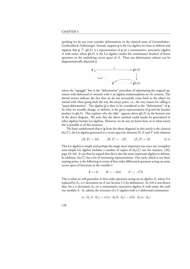
CHAPTER 5.

speaking we do not even consider deformations in the classical sense of Gerstenhaber–Grothendieck–Schlessinger. Instead, suppose g is the Lie algebra we want to deform andsuppose that g

ρ−→ gl(A) is a representation of g on a commutative, associative algebraA with unity, where gl(A) is the Lie algebra (under the commutator bracket) of linearoperators on the underlying vector space of A. Then our deformation scheme can bediagrammatically depicted as

gρ // gl(A)

OOO

g

"limit"

ee

// gl(A)xx

where the "squiggly" line is the "deformation" procedure of substituting the original op-erators with deformed (σ-twisted, with σ an algebra endomorphism on A) versions. Thedotted arrows indicate the fact that we do not necessarily come back to the object westarted with when going back the way the arrays point, i.e., the very reason for calling it“quasi-deformation”. The algebra g is then to be considered as the "deformation" of g.So what we actually change, or deform, is the given representation of g and the bracketproduct in gl(A). This explains why the tilde ˜ appears above gl(A) in the bottom rowof the above diagram. We note that the above method could maybe be generalized toother algebras besides Lie algebras. However, we do not yet know how, or to what extentthis is possible as of this moment.

The basic undeformed object (g from the above diagram) in this article is the classicalsl2(C), the Lie algebra generated as a vector space by elementsH,E and F with relations

〈H,E〉 = 2E, 〈H,F 〉 = −2F, 〈E,F 〉 = H. (5.1)

This Lie algebra is simple and perhaps the single most important one since any (complex)semi-simple Lie algebra includes a number of copies of sl2(C) (see for instance, [30],page 43–44). It can thus be argued that this is also the most important algebra to deform.In addition, sl2(C) has a lot of interesting representations. One such, which is our basicstarting point, is the following in terms of first order differential operators acting on somevector space of functions in the variable t:

E 7→ ∂, H 7→ −2t∂, F 7→ −t2∂.

This is what we will generalize to first order operators acting on an algebra A, where ∂ isreplaced by ∂σ , a σ-derivation on A (see Section 5.2 for definitions). In [16] it was shownthat, for a σ-derivation ∂σ on a commutative associative algebra A with unity, the rankone module A · ∂σ admits the structure of a C-algebra with a σ-deformed commutator

〈a · ∂σ, b · ∂σ〉 = σ(a) · ∂σ(b · ∂σ)− σ(b) · ∂σ(a · ∂σ)

128

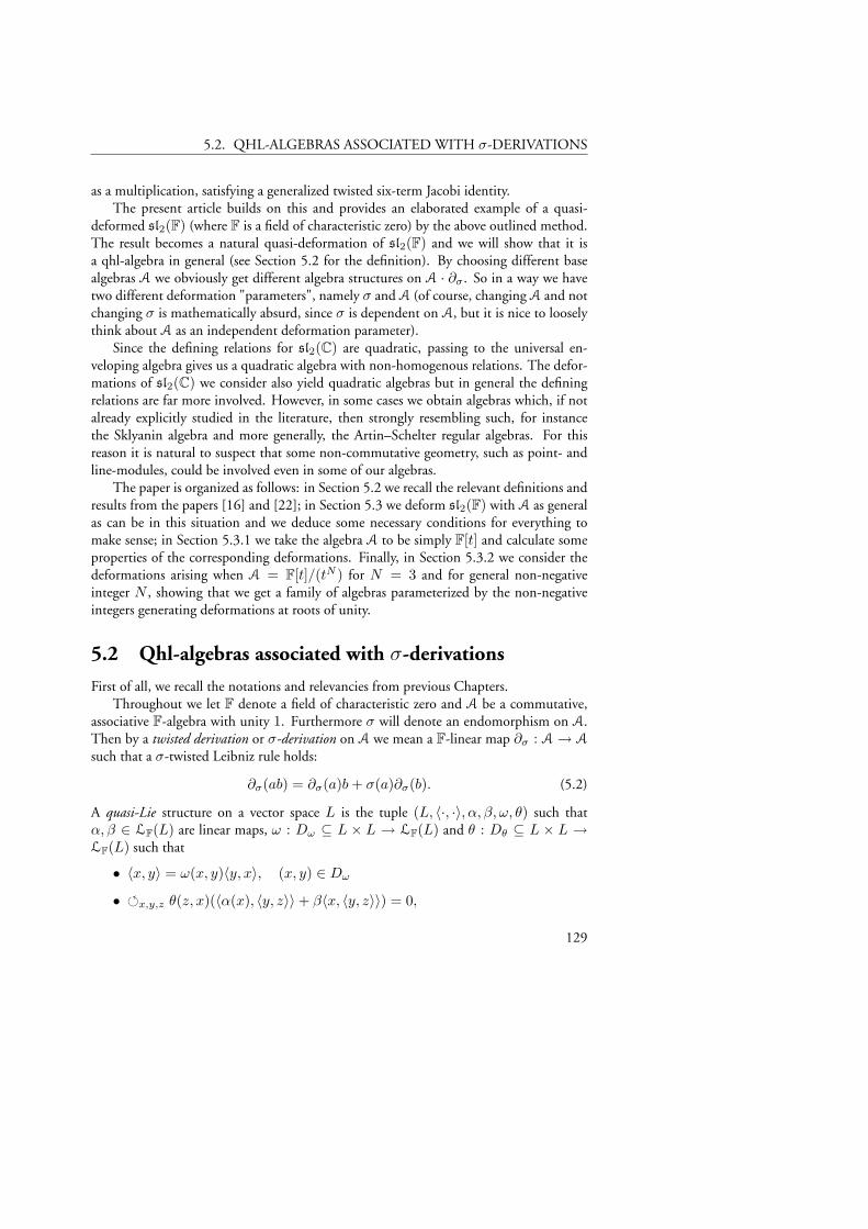
5.2. QHL-ALGEBRAS ASSOCIATED WITH σ-DERIVATIONS

as a multiplication, satisfying a generalized twisted six-term Jacobi identity.The present article builds on this and provides an elaborated example of a quasi-

deformed sl2(F) (where F is a field of characteristic zero) by the above outlined method.The result becomes a natural quasi-deformation of sl2(F) and we will show that it isa qhl-algebra in general (see Section 5.2 for the definition). By choosing different basealgebras A we obviously get different algebra structures on A · ∂σ . So in a way we havetwo different deformation "parameters", namely σ and A (of course, changing A and notchanging σ is mathematically absurd, since σ is dependent on A, but it is nice to looselythink about A as an independent deformation parameter).

Since the defining relations for sl2(C) are quadratic, passing to the universal en-veloping algebra gives us a quadratic algebra with non-homogenous relations. The defor-mations of sl2(C) we consider also yield quadratic algebras but in general the definingrelations are far more involved. However, in some cases we obtain algebras which, if notalready explicitly studied in the literature, then strongly resembling such, for instancethe Sklyanin algebra and more generally, the Artin–Schelter regular algebras. For thisreason it is natural to suspect that some non-commutative geometry, such as point- andline-modules, could be involved even in some of our algebras.

The paper is organized as follows: in Section 5.2 we recall the relevant definitions andresults from the papers [16] and [22]; in Section 5.3 we deform sl2(F) with A as generalas can be in this situation and we deduce some necessary conditions for everything tomake sense; in Section 5.3.1 we take the algebra A to be simply F[t] and calculate someproperties of the corresponding deformations. Finally, in Section 5.3.2 we consider thedeformations arising when A = F[t]/(tN ) for N = 3 and for general non-negativeinteger N , showing that we get a family of algebras parameterized by the non-negativeintegers generating deformations at roots of unity.

5.2 Qhl-algebras associated with σ-derivations

First of all, we recall the notations and relevancies from previous Chapters.Throughout we let F denote a field of characteristic zero and A be a commutative,

associative F-algebra with unity 1. Furthermore σ will denote an endomorphism on A.Then by a twisted derivation or σ-derivation on A we mean a F-linear map ∂σ : A → A

such that a σ-twisted Leibniz rule holds:

∂σ(ab) = ∂σ(a)b+ σ(a)∂σ(b). (5.2)

A quasi-Lie structure on a vector space L is the tuple (L, 〈·, ·〉, α, β, ω, θ) such thatα, β ∈ LF(L) are linear maps, ω : Dω ⊆ L × L → LF(L) and θ : Dθ ⊆ L × L →LF(L) such that

• 〈x, y〉 = ω(x, y)〈y, x〉, (x, y) ∈ Dω

• x,y,z θ(z, x)(〈α(x), 〈y, z〉〉+ β〈x, 〈y, z〉〉) = 0,

129

CHAPTER 5.

for x, y, z ∈ L and (z, x), (x, y), (y, z) ∈ Dθ. This definition includes quasi-hom-Lie algebras (which includes color Lie algebras and Lie super-algebras, for instance) if inaddition imposing the conditions 〈α(x), α(y)〉 = β α〈x, y〉 and ω = θ. If, further,β = id and ω = − id we get a hom-Lie algebra.

We let Derσ(A) denote the set of σ-derivations on A. Fixing a homomorphismσ : A → A, an element ∂σ ∈ Derσ(A), and an element δ ∈ A, we assume that theseobjects satisfy the following two conditions:

σ(Ann(∂σ)) ⊆ Ann(∂σ), (5.3)

∂σ(σ(a)) = δσ(∂σ(a)), for a ∈ A, (5.4)

where Ann(∂σ) := a ∈ A | a · ∂σ = 0. Let A · ∂σ = a · ∂σ | a ∈ A denote thecyclic A-submodule of Derσ(A) generated by ∂σ and extend σ to A · ∂σ by σ(a · ∂σ) =σ(a) · ∂σ . Recall the following theorem, from Chapter 3 which introduces a F-algebrastructure on A · ∂σ making it a quasi-hom-Lie algebra.

Theorem 5.1. If (5.3) holds then the map 〈·, ·〉σ defined by setting

〈a · ∂σ, b · ∂σ〉σ = (σ(a) · ∂σ) (b · ∂σ)− (σ(b) · ∂σ) (a · ∂σ), (5.5)

for a, b ∈ A and where denotes composition of maps, is a well-defined F-algebra product onthe F-linear space A · ∂σ . It satisfies the following identities for a, b, c ∈ A:

〈a · ∂σ, b · ∂σ〉σ = (σ(a)∂σ(b)− σ(b)∂σ(a)) · ∂σ, (5.6)

〈a · ∂σ, b · ∂σ〉σ = −〈b · ∂σ, a · ∂σ〉σ, (5.7)

and if, in addition, (5.4) holds, we have the deformed six-term Jacobi identity

a,b,c

(〈σ(a) · ∂σ, 〈b · ∂σ, c · ∂σ〉σ〉σ + δ · 〈a · ∂σ, 〈b · ∂σ, c · ∂σ〉σ〉σ

)= 0. (5.8)

5.3 Quasi-Deformations

Let A be a commutative, associative F-algebra with unity 1, t an element of A, and letσ denote an F-algebra endomorphism on A. Also, let Derσ(A) denote the linear spaceof σ-derivations on A. Choose an element ∂σ of Derσ(A) and consider the F-subspaceA · ∂σ of elements on the form a · ∂σ for a ∈ A. We will usually denote a · ∂σ simply bya∂σ . Notice that A · ∂σ is a left A-module. By Theorem 3.3 there is a skew-symmetricalgebra structure on this A-module given by

〈a · ∂σ, b · ∂σ〉 = σ(a) · ∂σ(b · ∂σ)− σ(b) · ∂σ(a · ∂σ) == σ(a∂σ)(b∂σ)− σ(b∂σ)(a∂σ) = (σ(a)∂σ(b)− σ(b)∂σ(a)) · ∂σ, (5.9)

130

5.3. QUASI-DEFORMATIONS

where a, b ∈ A and σ is extended to a map on A · ∂σ by σ(a∂σ) = σ(a)∂σ . Theelements e := ∂σ, h := −2t∂σ and f := −t2∂σ span an F-linear subspace

S := LinSpanF∂σ,−2t∂σ,−t2∂σ = LinSpanFe, h, f

of A · ∂σ . We restrict the multiplication (5.9) to S without, at this point, assumingclosure. Now,

∂σ(t2) = ∂σ(t · t) = σ(t)∂σ(t) + ∂σ(t)t = (σ(t) + t)∂σ(t)

which by using (5.9), leads to

〈h, f〉 = 2〈t∂σ, t2∂σ〉 = 2σ(t)∂σ(t)t∂σ, (5.10a)

〈h, e〉 = −2〈t∂σ, ∂σ〉 = −2(σ(t)∂σ(1)− σ(1)∂σ(t))∂σ, (5.10b)

〈e, f〉 = −〈∂σ, t2∂σ〉 = −(σ(1)(σ(t) + t)∂σ(t)− σ(t)2∂σ(1))∂σ. (5.10c)

Also, one would be tempted to make the general ansatz

∂σ(1) = d0 + d1t+ · · ·+ dktk, σ(1) = s0 + s1t+ · · ·+ slt

l.

If all non-negative integer powers of t are linearly independent over F, then σ(1) = 1 orσ(1) = 0 since σ(1) = σ(1 · 1) = σ(1)2 and so s0 is either 1 or 0 and

s1 = · · · = sl = 0.

In addition to this, in this case,

d0 + d1t+ · · ·+ dktk = ∂σ(1) = ∂σ(1 · 1) = σ(1)∂σ(1) + ∂σ(1)1 =

= (σ(1) + 1)∂σ(1) = (s0 + 1)(d0 + d1t+ · · ·+ dktk)

leading to d0 = d1 = · · · = dk = 0 if s0 = 1 and arbitrary d0, . . . , dk if s0 = 0. But ifs0 = 0, that is σ(1) = 0, then σ(tw) = 0 for all w ∈ N since

σ(tw) = σ(1 · tw) = σ(1)σ(tw) = 0.

Under the assumptions σ(1) = 1 and ∂σ(1) = 0 relations (5.10a), (5.10b) and (5.10c)simplify to

〈h, f〉 = 2σ(t)∂σ(t)t∂σ (5.11a)

〈h, e〉 = 2∂σ(t)∂σ (5.11b)

〈e, f〉 = −(σ(t) + t)∂σ(t)∂σ. (5.11c)

Remark 23. Note that when σ = id and ∂σ(t) = 1 we retain the classical sl2(F) withrelations (5.1).

131

CHAPTER 5.

5.3.1 Quasi-Deformations with base algebra A = F[t]

Take A to be the polynomial algebra F[t], σ(1) = 1 and ∂σ(1) = 0. Since all non-negative integer powers of t are linearly independent over F in F[t], we are in the situationof relations (5.10a), (5.10b) and (5.10c). Suppose that σ(t) = q(t) and ∂σ(t) = p(t),where p(t), q(t) ∈ F[t]. To have closure of (5.11a), (5.11b) and (5.11c) these polynomi-als are far from arbitrary. Indeed, by (5.11a) we get

deg(∂σ(t)σ(t)) = deg(p(t)q(t)) ≤ 1.

So three cases arise

Case 1: σ(t) = q(t) = q0 + q1t, q1 6= 0, p(t) = p0,

Case 2: σ(t) = q(t) = q0, q0 6= 0, p(t) = p0 + p1t,

Case 3: σ(t) = q(t) = 0, p(t) = p0 + p1t+ · · ·+ pntn,

where in all three cases we assume p(t) 6= 0. Note that if p(t) = 0 then ∂σ = 0 and sothe original operator representation collapses.

Remark 24. If we allow σ(t) = q(t) and ∂σ(t) = p(t) where p, q are arbitrary polyno-mials in t then we get a deformation of sl2(F) which does not preserve dimension; that is,brackets of the basis elements e, f, h are not simply linear combinations in these elementsbut include more new "basis" elements. This phenomena could possibly be interesting tostudy further.

Case 1: Assume q(t) = q0 + q1t, implying that p(t) = p0. Relations (5.11a), (5.11b)and (5.11c) according to (5.9) now become

〈h, f〉 : −2q0ef + q1hf + q20eh− q0q1h2 − q21fh = −q0p0h− 2q1p0f (5.12a)

〈h, e〉 : −2q0e2 + q1he− eh = 2p0e (5.12b)

〈e, f〉 : ef + q20e2 − q0q1he− q21fe = −q0p0e+

q1 + 12

p0h. (5.12c)

Remark 25. Notice that changing the role of h and f in (5.12a) does not correspondto changing h and f in (5.9). This means that, in a sense, the skew-symmetry of (5.9)is "hidden" in (5.12a). If 〈f, h〉 is calculated from (5.9) one sees that indeed 〈f, h〉 =−〈h, f〉 as one would expect and one gets exactly minus the left-hand-side of (5.12a).

Henceforth, we denote by Fx1, . . . , xn the free associative algebra over F on theset x1, . . . , xn, i.e., the non-commutative polynomial (tensor) algebra over F in theindeterminates x1, . . . , xn.

132

5.3. QUASI-DEFORMATIONS

The associative algebra with three abstract generators e, h and f and defining relations(5.12a), (5.12b) and (5.12c), that is, Fe, f, h modulo the relations defined by (5.12a),(5.12b) and (5.12c), can be seen as a multi-parameter deformation of

U(sl2(F)) = Fe, f, h/ (

[h, e]− 2e, [h, f ] + 2f, [e, f ]− h),

where [·, ·] denotes the commutator.

Example 21. By taking q0 = 0 and q := q1 6= 0 we obtain a deformation of sl2(F)corresponding to replacing the ordinary derivation operator with the Jackson q-derivativeDq (see Section 5.2). Since this deformation therefore is quite interesting we explicitlyrecord it

hf − qfh = −2p0f

he− q−1eh = 2q−1p0e (5.13)

ef − q2fe =q + 1

2p0h.

Note that, by taking p0 = q = 1, we obtain the usual commutation relations for sl2(F),corresponding to the ordinary derivation operator ∂. We denote the "lifting" of the right-hand-side of (5.12a), (5.12b), (5.12c) for p0 = 1, q0 = 0, to an abstract skew-symmetricalgebra with products

〈h, f〉 = −2qf, 〈h, e〉 = 2e, 〈e, f〉 =q + 1

2h,

by qsl2(F) and call it informally the "Jackson sl2(F)". In Example 24 we will see thatqsl2(F) is a (quasi-) hom-Lie algebra. When p0 6= 1 we get a natural one-parameterdeformation of qsl2(F). The algebra Fe, f, h/(5.13), with p0 = 1 in (5.13), can bethought of as an analogue of the universal enveloping algebra for qsl2(F). For q = 1 it isindeed the universal enveloping algebra of the Lie algebra sl2(F). We denote by Uq thealgebra Fe, f, h/(5.13). When p0 6= 1 we similarly get a one-parameter deformationof Uq.

There is also a Casimir-like element in this algebra, namely,

Ωq := ef + qfe+q + 1

4h2 = ef + qfe+

2q

4h2.

For q = 1 we retain the classical central Casimir element for U(sl2(F)) in the basise, f, h. It is straightforward to check that Ωq is normal in the sense that τ(z)·Ωq = Ωq ·zfor some map τ (notice that in the Lie case q = 1 the element Ω1 is really central, i.e.,τ = id). The associative product in Uq forces τ to be an algebra endomorphism. Indeed,on the one hand: Ωq · zw = τ(z) · Ωq · w = τ(z)τ(w) · Ωq, and on the other:Ωq · zw = τ(zw) · Ωq. It can also be checked that τ is in fact an automorphism.In our present setting τ is completely determined by its action on the basis elements asτ(e) = q−2e, τ(h) = h and τ(f) = q2f .

133

CHAPTER 5.

Remark 26. Assume that q 6= 1 and rewrite the relations (5.13) in the form:

yz − q−1zy = 0

zx− q2xz = p20(1 + q−1)y + p2

0

q + 1q − 1

1

xy − q−1yx = 0,

(5.14)

where we made the transformations h 7→ 2p0q−1y− 2p0/(q− 1)1, f 7→ x and e 7→ z.

Since the transformation is a bijection (it is simply a change of basis) we deduce thatFe, f, h/(5.13) and Fx, y, z/(5.14) are isomorphic as algebras. We denote thealgebra Fx, y, z/(5.14) by Wq. Hence Wq

∼= Uq. It is easy to see that Wq is aniterated Ore extension as follows. Indeed, putting

B := Fy, z/(yz − q−1zy)

we see that this is an Ore extension of F[z] with automorphism z 7→ q−1z. Thenextending once more we get Wq as the Ore extension B[x, ς, ∂ς ] of B defined by ς(z) =q−2z, ∂ς(z) = −q−2ay − q−2b1, ς(y) = q−1y and ∂ς(y) = 0. (What is neededto check is that ∂ς(yz) and ∂ς(q−1zy) both give the same result.) We now note thatiterated Ore extensions of an Auslander-regular algebra (see below for the definition), inthis case F[z], are themselves Auslander-regular by a theorem of Ekström [11]. Moreover,one can prove ([3], Proposition 2.1.1) that Wq has global dimension at most three. Also,using Proposition 2.1.2 in [3] or the Diamond Lemma [17] it is easy to check that Wq

has a PBW-basis, hence is a noetherian domain of Gel’fand–Kirillov dimension three ([3],Proposition 2.1.1). Having a PBW-basis ensures Koszulity as an almost quadratic algebra[29]. We note the following interesting special case of relations (5.14).

Example 22. When q = −1 the endomorphism σ becomes σ(t) = −t and the Jacksonq-derivative is thus given by f 7→ (f(t) − f(−t))/2t. The defining relations (5.14) forW−1 then become

yz + zy = 0, zx− xz = 0, xy + yx = 0. (5.15)

This is in fact a color-commutative Lie algebra graded by Z22. Indeed, suppose we have a

vector space V with decomposition

V = V(0,0) ⊕ V(1,0) ⊕ V(0,1) ⊕ V(1,1) = F0 ⊕ Fy ⊕ F0 ⊕(Fx⊕ Fz

).

Taking the colored commutator [A,B]col := AB − (−1)(deg(A),deg(B))BA, wherewe have the bilinear form (·, ·) defined by (deg(A),deg(B)) := α1β1 + α2β2 fordeg(A) = (α1, α2) and deg(B) = (β1, β2) yields the algebra defined by relations(5.15).

134

5.3. QUASI-DEFORMATIONS

Homogenizing the relations (5.12a), (5.12b) and (5.12c) with respect to a centraldegree-one element ζ leads to algebras reminiscent of the central extensions of three-dimensional Artin–Schelter regular algebras (in particular the Sklyanin algebra) studied(among other algebras) in [25]. The Artin–Schelter regular algebras with homogeneousdefining relations (and more generally Auslander-regular algebras) turned out to be a mostnatural choice for a non-commutative projective geometry and this stimulated a directedeffort in understanding the various homological and geometric properties of these algebras(see [1], [2], [25], for instance). Also, let g be a finite-dimensional Lie algebra. Thenthe universal enveloping algebra U(g) is filtered by the canonical degree-filtration. Thisis a Zariski-filtration and since gr(U(g)) is isomorphic to a commutative polynomialalgebra (by the PBW-theorem) this being Auslander-regular, it follows that U(g) is itselfAuslander-regular [28]. Le Bruyn and Smith, Le Bruyn and Van den Bergh, showedthat U(g) (or rather its homogenizations) is connected to non-commutative projectivealgebraic geometry [24], [26].

For the reader’s convenience we recall the definition of Artin–Schelter regular andAuslander-regular algebras. Let R be a graded connected algebra over a field F, i.e.,R =

⊕n∈Z≥0

Rn with R0∼= F. Then R is Artin–Schelter regular (AS-regular) if it has

finite global dimension d (all graded R-modules have finite projective dimension ≤ d)and

• R has finite Gel’fand–Kirillov dimension, that is, if it has polynomial growth, i.e.,if dimF(Rn) ≤ nk, for some constant k ∈ N;

• R is Gorenstein: ExtiR(F, R) = 0 if i 6= d and Extd

R(F, R) ∼= F.

A related concept is the Auslander-regular algebras. Let R be a noetherian ring. ThenR is said to be Auslander-regular if for every R-module M and for all submodules N ofExti

R(M, R) we have minj | ExtjR(N, R) 6= 0 ≥ i, ∀ i ≥ 0, in addition to R

having finite injective and global dimension. For graded algebras of Gel’fand–Kirillovdimension less than or equal to three it has been shown by Thierry Levasseur [27] thatAuslander-regular and AS-regular are in fact equivalent.

We now review the notion of conformal sl2(F) enveloping algebras introduced byLieven Le Bruyn in [23], showing that Uq defined by (5.13) also is a special case of hisconstruction.

Example 23. Let a denote the C-vector (a1, a2, a3, a4, a5, a6, a7). Define an algebra

F(a) := Cx, y, z/ xy − a1yx− a2y,

yz − a3zy − a4x2 − a5x,

zx− a6xz − a7z

.

Notice that, for instance, F(1, 2, 1, 0, 1, 1, 2) ∼= U(sl2(C)). Therefore it is temptingto view F(a), for generic a’s, as deformations of U(sl2(C)). Such a deformation of

135

CHAPTER 5.

U(sl2(C)) is called a conformal sl2 enveloping algebra if gr(F(a)), with F(a) taken withthe canonical degree-filtration, is a three-dimensional Auslander-regular quadratic alge-bra. Edward Witten introduced a special case of the above, namely the algebra

Wa := F(a, 1, 1, a− 1, 1, a, 1) = Cx, y, z/ xy − ayx− y,

yz − zy − (a− 1)x2 − x,zx− axz − z

related to some aspects of two-dimensional conformal field theory. The case a = 1 givesan algebra isomorphic to U(sl2(C)).

Suppose a1a2a3a5a6a7 6= 0. Le Bruyn shows that under this condition F(a) is aconformal sl2(C) enveloping algebra if and only if a6 = a1 and a7 = a2.

We now note that when F = C our algebra Uq is a conformal sl2(C) envelopingalgebra. In fact Uq = F(a′), under the assignments h 7→ x, e 7→ y, f 7→ z and where

a′ = (q−1, 2q−1p0, q2, 0,

q + 12

p0, q−1, 2q−1p0).

This also shows that Uq is Auslander-regular since a1 = a6 and a2 = a7. Le Bruyn alsoshows in [23] that there is a very nice non-commutative geometry behind these algebraswhen homogenized.

By taking p0 = q0 = 0 in (5.13) we get an “abelianized” version of qsl2(F). However,as we mentioned before, the operator representation we started with collapses in this casesince ∂σ = 0.

Remark 27. Note that, unlike the undeformed U(sl2(F)), the one-parameter defor-mation of Uq (with q 6= 1, p0 6= 0) has non-trivial one-dimensional representations.

Indeed, taking h = 2p0/(q − 1) we see from the defining relations that ef = − p20

(q−1)2

and so e and f can be chosen as any numbers satisfying this equality. When q → 1 inwhich case we “approach sl2(F)” we see that h goes to infinity and so the representationcollapses in the limit.

Remark 28. It is important to notice that Theorem 3.3 gives us two alternative ways toview our algebras:

(i) either one uses Theorem 3.3 to construct a bracket on the vector space A · ∂σ withthe help of equation (3.21), viewing this bracket as a product;

(ii) or one uses (3.21) in adjunction with the definition (3.20) of the bracket to obtainquadratic relations and “moding” out these from the tensor algebra, thereby givingus an associative quadratic algebra which loosely can be thought of as a deformed“enveloping algebra” of the corresponding algebra from viewpoint (i), or even as adeformed universal enveloping algebra for sl2(F).

136

5.3. QUASI-DEFORMATIONS

Twisted Jacobi identity for Case 1

The possible δ ∈ A = F[t] in the twisted Jacobi identity can be computed from thecondition

∂σ σ(a) = δ · σ ∂σ(a), (5.16)

required to hold for any a ∈ A. For a = t0 = 1 this equation holds trivially becauseσ(1) = 1 and ∂σ(1) = 0. For a = t the left-hand-side becomes

∂σ σ(t) = ∂σ(q0 + q1t) = q1p0

and the right-hand-side becomes

δ · σ ∂σ(t) = δ · σ(p0) = δ · p0,

from which we immediately see that δ = q1. To show that (5.16) holds for all a ∈ A

with δ = q1 it is enough by linearity to show this for arbitrary monomial a = tk. As wehave seen the statement is true for k = 0, 1. Assume the statement holds for k = l. Onwriting tl+1 = ttl and using the σ-Leibniz rule (5.2) we get:

R.H.S = δ · σ ∂σ(tl+1) = δ · (σ ∂σ(t)σ(t)l + σ2(t)σ ∂σ(tl)) =

= δ · σ ∂σ(t)σ(tl) + σ2(t) · δ · σ ∂σ(tl) = [induction step] =

= (∂σ σ(t))σ(tl) + σ2(t)∂σ σ(tl) = ∂σ σ(tl+1) = L.H.S.

Note that this shows that it is enough to check condition (5.16) for low degrees, even incases other than the present. So by Theorem 3.3 we now have a deformed Jacobi identity

x,y,z (〈σ(x), 〈y, z〉〉+ q1〈x, 〈y, z〉〉) = 0

on A · ∂σ = F[t] · ∂σ . By defining α(x) := q−11 σ(x) this can be re-written as the

Jacobi-like relation for a hom-Lie algebra

x,y,z 〈(α+ id)(x), 〈y, z〉〉 = 0. (5.17)

Note that this twisted Jacobi identity follows directly from the general Theorem 3.3. Thisshows that we do not have to make any lengthy trial computations with different moreor less ad hoc assumptions on the form of the identity.

Example 24. The algebra qsl2(F) is a hom-Lie algebra with α = q−1σ and with Jacobiidentity as given by (5.17). This is not clear à priori since qsl2(F) is not a subalgebra ofA · ∂σ . When qsl2(F) is represented by its "non-lifted" operators e = ∂σ, h = −2t∂σ

and f = −t2∂σ , this representation becomes a subalgebra of A ·∂σ and hence a hom-Lie

137

CHAPTER 5.

algebra. However, qsl2(F) is defined abstractly without reference to a particular repre-sentation. It is initially possible that the twisted Jacobi identity is a result of some extrarelations (e.g., by the σ-Leibniz rule) available in that representation as σ-derivations.

To prove that qsl2(F) is a hom-Lie algebra we proceed as follows. First define α onthe basis vectors e, f, h as α(e) = q−1e, α(h) = h and α(f) = qf . It is clear that it isenough to consider the case when x = e, y = f and z = h. Then (5.17) becomes

〈(α+ id)(e),〈f, h〉〉+ 〈(α+ id)(f), 〈h, e〉〉+ 〈(α+ id)(h), 〈e, f〉〉 =

= 2q(q−1 + 1)〈e, f〉+ 2(q + 1)〈f, e〉+ (q + 1)〈h, h〉 == (2(q + 1)− 2(q + 1))〈e, f〉 = 0,

where we have used that 〈·, ·〉 is skew-symmetric.

Case 2: Assume now that σ(t) = q(t) = q0 6= 0 and so ∂σ(t) = p(t) = p0 + p1t. Therelations (5.11a), (5.11b) and (5.11c) combined with (5.9) become

〈h, f〉 : −2ef + q0eh = −p0h− 2p1f

〈h, e〉 : −2q0e2 − eh = 2p0e− p1h

〈e, f〉 : ef + q20e2 = −q0p0e+

q0p1 + p0

2h+ p1f,

since σ(e) = e, σ(h) = −2q0e and σ(f) = −q20e. It is obvious that we cannot recoverthe classical sl2(F) from this deformation by specifying suitable parameters since, in asense, the commutators "collapsed" due to the choice of σ.

Twisted Jacobi identity for Case 2

It is easy to deduce, following the same arguments as in Case 1, that one can take δ = 0in this case and so have

x,y,z 〈σ(x), 〈y, z〉〉 = 0 (5.19)

on A · ∂σ making it into a hom-Lie algebra.

Case 3: It follows immediately upon insertion of ∂σ(t) = p(t) = p0 + p1t+ · · ·+ pntn

into (5.11c) that deg(p(t)) ≤ 1. With this (5.11a), (5.11b) and (5.11c) combined with(5.9) now become

0 = 0, −eh = 2p0e− p1h, ef =p0

2h+ p1f.

Twisted Jacobi identity for Case 3

In this case (5.16) becomes 0 = ∂σ(0) = ∂σ(σ(tk)) = δ · σ(∂σ(tk)) = δ · 0, valid forall k ∈ Z≥0, and so δ can be chosen completely arbitrary in this case, for example δ = 0giving again (5.19) and thus a hom-Lie algebra.

138

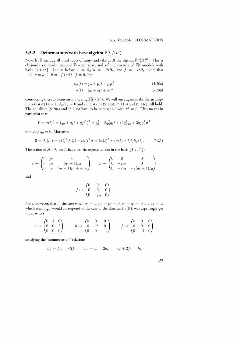
5.3. QUASI-DEFORMATIONS

5.3.2 Deformations with base algebra F[t]/(t3)

Now, let F include all third roots of unity and take as A the algebra F[t]/(t3). This isobviously a three-dimensional F-vector space and a finitely generated F[t]-module withbasis 1, t, t2. Let, as before, e = ∂σ, h = −2t∂σ, and f = −t2∂σ. Note that−2t · e = h, t · h = 2f and t · f = 0. Put

∂σ(t) = p0 + p1t+ p2t2 (5.20a)

σ(t) = q0 + q1t+ q2t2 (5.20b)

considering these as elements in the ring F[t]/(t3). We will once again make the assump-tions that σ(1) = 1, ∂σ(1) = 0 and so relations (5.11a), (5.11b) and (5.11c) still hold.The equalities (5.20a) and (5.20b) have to be compatible with t3 = 0. This means inparticular that

0 = σ(t)3 = (q0 + q1t+ q2t2)3 = q30 + 3q20q1t+ (3q20q2 + 3q0q21)t2

implying q0 = 0. Moreover,

0 = ∂σ(t3) = σ(t)2∂σ(t) + ∂σ(t2)t = (σ(t)2 + (σ(t) + t)t)∂σ(t). (5.21)

The action of A · ∂σ on A has a matrix representation in the basis 1, t, t2:

e 7→

0 p0 00 p1 (q1 + 1)p0

0 p2 (q1 + 1)p1 + q2p0

, h 7→

0 0 00 −2p0 00 −2p1 −2(q1 + 1)p0

and

f 7→

0 0 00 0 00 −p0 0

.

Note, however, that in the case when p0 = 1, p1 = p2 = 0, q0 = q2 = 0 and q1 = 1,which seemingly would correspond to the case of the classical sl2(F), we surprisingly getthe matrices

e 7→

0 1 00 0 20 0 0

, h 7→

0 0 00 −2 00 0 −4

, f 7→

0 0 00 0 00 −1 0

satisfying the "commutation" relations

hf − fh = −2f, he− eh = 2e, ef + 2fe = h.

139

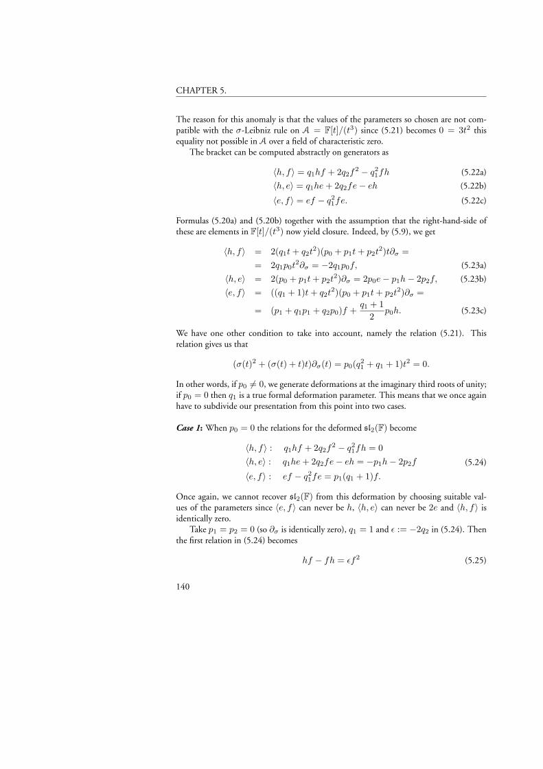
CHAPTER 5.

The reason for this anomaly is that the values of the parameters so chosen are not com-patible with the σ-Leibniz rule on A = F[t]/(t3) since (5.21) becomes 0 = 3t2 thisequality not possible in A over a field of characteristic zero.

The bracket can be computed abstractly on generators as

〈h, f〉 = q1hf + 2q2f2 − q21fh (5.22a)

〈h, e〉 = q1he+ 2q2fe− eh (5.22b)

〈e, f〉 = ef − q21fe. (5.22c)

Formulas (5.20a) and (5.20b) together with the assumption that the right-hand-side ofthese are elements in F[t]/(t3) now yield closure. Indeed, by (5.9), we get

〈h, f〉 = 2(q1t+ q2t2)(p0 + p1t+ p2t

2)t∂σ == 2q1p0t

2∂σ = −2q1p0f, (5.23a)

〈h, e〉 = 2(p0 + p1t+ p2t2)∂σ = 2p0e− p1h− 2p2f, (5.23b)

〈e, f〉 = ((q1 + 1)t+ q2t2)(p0 + p1t+ p2t

2)∂σ =

= (p1 + q1p1 + q2p0)f +q1 + 1

2p0h. (5.23c)

We have one other condition to take into account, namely the relation (5.21). Thisrelation gives us that

(σ(t)2 + (σ(t) + t)t)∂σ(t) = p0(q21 + q1 + 1)t2 = 0.

In other words, if p0 6= 0, we generate deformations at the imaginary third roots of unity;if p0 = 0 then q1 is a true formal deformation parameter. This means that we once againhave to subdivide our presentation from this point into two cases.

Case 1: When p0 = 0 the relations for the deformed sl2(F) become

〈h, f〉 : q1hf + 2q2f2 − q21fh = 0〈h, e〉 : q1he+ 2q2fe− eh = −p1h− 2p2f

〈e, f〉 : ef − q21fe = p1(q1 + 1)f.

(5.24)

Once again, we cannot recover sl2(F) from this deformation by choosing suitable val-ues of the parameters since 〈e, f〉 can never be h, 〈h, e〉 can never be 2e and 〈h, f〉 isidentically zero.

Take p1 = p2 = 0 (so ∂σ is identically zero), q1 = 1 and ε := −2q2 in (5.24). Thenthe first relation in (5.24) becomes

hf − fh = εf2 (5.25)

140

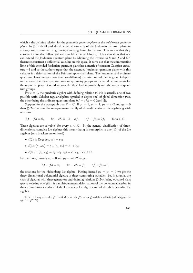
5.3. QUASI-DEFORMATIONS

which is the defining relation for the Jordanian quantum plane or the ε-deformed quantumplane. In [5] is developed the differential geometry of the Jordanian quantum plane inanalogy with commutative geometry’s moving frame formalism. This means that theyconstruct a suitable differential calculus (differential 1-forms). They also show that onecan extend the Jordanian quantum plane by adjoining the inverses to h and f and fur-thermore construct a differential calculus on this space. It turns out that the commutativelimit of this extended Jordanian quantum plane has a metric of constant Gaussian curva-ture −1 and so the authors argue that the extended Jordanian quantum plane with thiscalculus is a deformation of the Poincaré upper-half plane. The Jordanian and ordinaryquantum planes are both associated to (different) quantizations of the Lie group GL2(F)in the sense that these quantizations are symmetry groups with central determinants forthe respective plane. Considerations like these lead unavoidably into the realm of quan-tum groups.

For ε = 1, the quadratic algebra with defining relation (5.25) is actually one of twopossible Artin–Schelter regular algebras (graded in degree one) of global dimension two,the other being the ordinary quantum plane hf − qfh = 0 (see [1]).

Suppose for this paragraph that F = C. If q1 = 1, p1 = 1, p2 = a/2 and q2 = 0then (5.24) become the one-parameter family of three-dimensional Lie algebras g withrelations:

hf − fh = 0, he− eh = −h− af, ef − fe = 2f, for a ∈ C.

These algebras are solvable1 for every a ∈ C. By the general classification of three-dimensional complex Lie algebras this means that g is isomorphic to one [15] of the Liealgebras (zero brackets are omitted)

• `(2)⊕ Ce3: 〈e1, e2〉 = e2;

• `(3): 〈e1, e2〉 = e2, 〈e1, e3〉 = e2 + e3;

• `(3, c): 〈e1, e2〉 = e2, 〈e1, e3〉 = c · e3, for c ∈ C.

Furthermore, putting p1 = 0 and p2 = −1/2 we get

hf − fh = 0, he− eh = f, ef − fe = 0,

the relations for the Heisenberg Lie algebra. Putting instead p1 = p2 = 0 we get thethree-dimensional polynomial algebra in three commuting variables. So, in a sense, theclass of algebras with three generators and defining relations (5.24), being obtained via aspecial twisting of sl2(F), is a multi-parameter deformation of the polynomial algebra inthree commuting variables, of the Heisenberg Lie algebra and of the above solvable Liealgebra.

1In fact, it is easy to see that g(2) = 0 where we put g(1) = 〈g, g〉 and then inductively defining g(i) =〈g(i−1), g(i−1)〉.

141

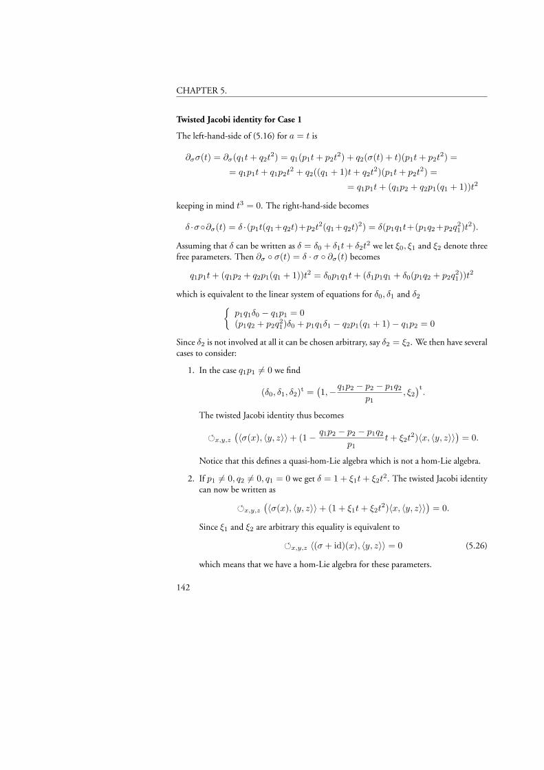
CHAPTER 5.

Twisted Jacobi identity for Case 1

The left-hand-side of (5.16) for a = t is

∂σσ(t) = ∂σ(q1t+ q2t2) = q1(p1t+ p2t

2) + q2(σ(t) + t)(p1t+ p2t2) =

= q1p1t+ q1p2t2 + q2((q1 + 1)t+ q2t

2)(p1t+ p2t2) =

= q1p1t+ (q1p2 + q2p1(q1 + 1))t2

keeping in mind t3 = 0. The right-hand-side becomes

δ ·σ∂σ(t) = δ ·(p1t(q1+q2t)+p2t2(q1+q2t)2) = δ(p1q1t+(p1q2+p2q

21)t2).

Assuming that δ can be written as δ = δ0 + δ1t+ δ2t2 we let ξ0, ξ1 and ξ2 denote three

free parameters. Then ∂σ σ(t) = δ · σ ∂σ(t) becomes

q1p1t+ (q1p2 + q2p1(q1 + 1))t2 = δ0p1q1t+ (δ1p1q1 + δ0(p1q2 + p2q21))t2

which is equivalent to the linear system of equations for δ0, δ1 and δ2p1q1δ0 − q1p1 = 0(p1q2 + p2q

21)δ0 + p1q1δ1 − q2p1(q1 + 1)− q1p2 = 0

Since δ2 is not involved at all it can be chosen arbitrary, say δ2 = ξ2. We then have severalcases to consider:

1. In the case q1p1 6= 0 we find

(δ0, δ1, δ2)t =(1,−q1p2 − p2 − p1q2

p1, ξ2

)t.

The twisted Jacobi identity thus becomes

x,y,z

(〈σ(x), 〈y, z〉〉+ (1− q1p2 − p2 − p1q2

p1t+ ξ2t

2)〈x, 〈y, z〉〉)

= 0.

Notice that this defines a quasi-hom-Lie algebra which is not a hom-Lie algebra.

2. If p1 6= 0, q2 6= 0, q1 = 0 we get δ = 1 + ξ1t+ ξ2t2. The twisted Jacobi identity

can now be written as

x,y,z

(〈σ(x), 〈y, z〉〉+ (1 + ξ1t+ ξ2t

2)〈x, 〈y, z〉〉)

= 0.

Since ξ1 and ξ2 are arbitrary this equality is equivalent to

x,y,z 〈(σ + id)(x), 〈y, z〉〉 = 0 (5.26)

which means that we have a hom-Lie algebra for these parameters.

142

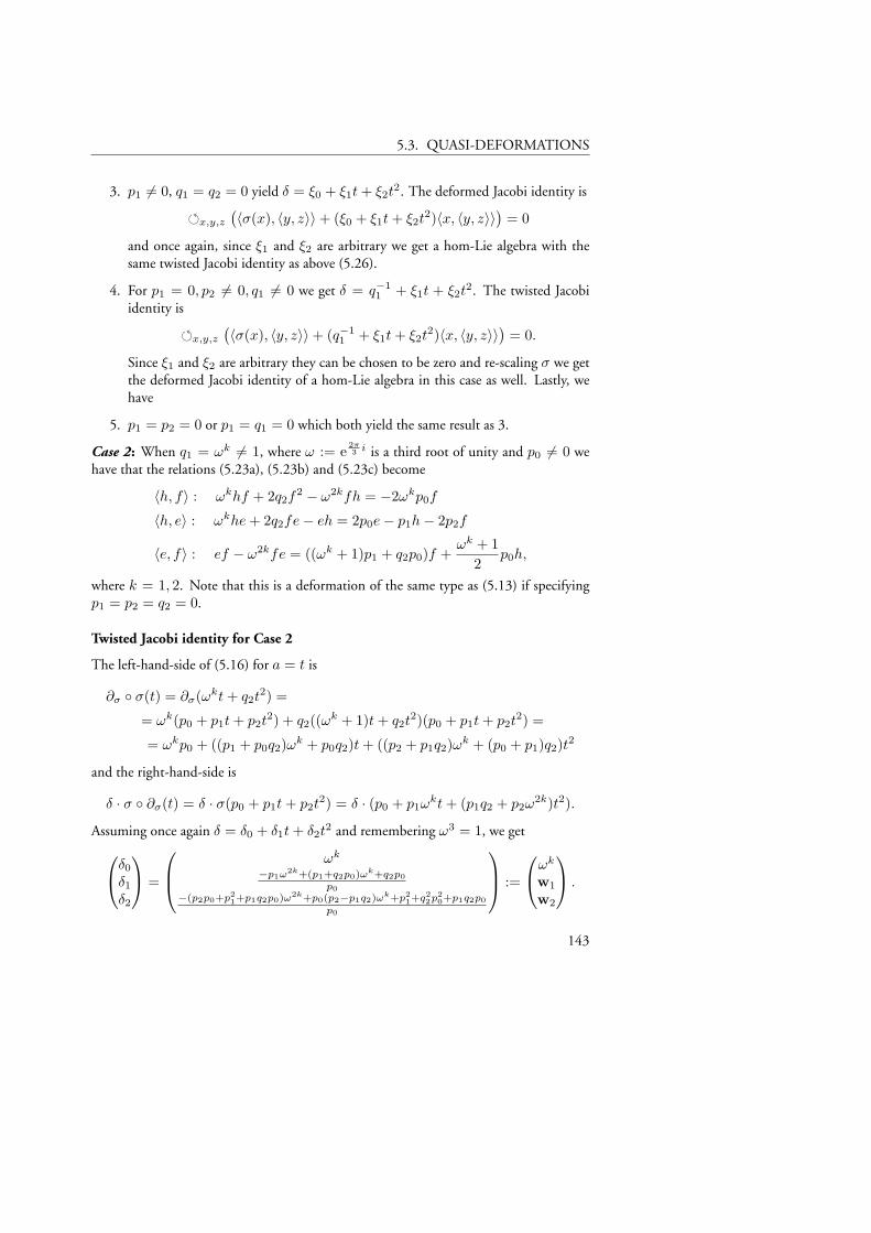
5.3. QUASI-DEFORMATIONS

3. p1 6= 0, q1 = q2 = 0 yield δ = ξ0 + ξ1t+ ξ2t2. The deformed Jacobi identity is

x,y,z

(〈σ(x), 〈y, z〉〉+ (ξ0 + ξ1t+ ξ2t

2)〈x, 〈y, z〉〉)

= 0

and once again, since ξ1 and ξ2 are arbitrary we get a hom-Lie algebra with thesame twisted Jacobi identity as above (5.26).

4. For p1 = 0, p2 6= 0, q1 6= 0 we get δ = q−11 + ξ1t + ξ2t

2. The twisted Jacobiidentity is

x,y,z

(〈σ(x), 〈y, z〉〉+ (q−1

1 + ξ1t+ ξ2t2)〈x, 〈y, z〉〉

)= 0.

Since ξ1 and ξ2 are arbitrary they can be chosen to be zero and re-scaling σ we getthe deformed Jacobi identity of a hom-Lie algebra in this case as well. Lastly, wehave

5. p1 = p2 = 0 or p1 = q1 = 0 which both yield the same result as 3.

Case 2: When q1 = ωk 6= 1, where ω := e2π3 i is a third root of unity and p0 6= 0 we

have that the relations (5.23a), (5.23b) and (5.23c) become

〈h, f〉 : ωkhf + 2q2f2 − ω2kfh = −2ωkp0f

〈h, e〉 : ωkhe+ 2q2fe− eh = 2p0e− p1h− 2p2f

〈e, f〉 : ef − ω2kfe = ((ωk + 1)p1 + q2p0)f +ωk + 1

2p0h,

where k = 1, 2. Note that this is a deformation of the same type as (5.13) if specifyingp1 = p2 = q2 = 0.

Twisted Jacobi identity for Case 2

The left-hand-side of (5.16) for a = t is

∂σ σ(t) = ∂σ(ωkt+ q2t2) =

= ωk(p0 + p1t+ p2t2) + q2((ωk + 1)t+ q2t

2)(p0 + p1t+ p2t2) =

= ωkp0 + ((p1 + p0q2)ωk + p0q2)t+ ((p2 + p1q2)ωk + (p0 + p1)q2)t2

and the right-hand-side is

δ · σ ∂σ(t) = δ · σ(p0 + p1t+ p2t2) = δ · (p0 + p1ω

kt+ (p1q2 + p2ω2k)t2).

Assuming once again δ = δ0 + δ1t+ δ2t2 and remembering ω3 = 1, we getδ0δ1

δ2

=

ωk

−p1ω2k+(p1+q2p0)ωk+q2p0

p0−(p2p0+p2

1+p1q2p0)ω2k+p0(p2−p1q2)ω

k+p21+q2

2p20+p1q2p0

p0

:=

ωk

w1

w2

.

143

CHAPTER 5.

The deformed Jacobi identity can thus be written in the following form

x,y,z

(〈σ(x), 〈y, z〉〉+ (ωk + w1t+ w2t

2)〈x, 〈y, z〉〉)

= 0,

this being the defining relation for a quasi-hom-Lie algebra. This quasi-hom-Lie algebrabecomes a hom-Lie algebra when w1 = w2 = 0, that is for some special choices ofparameters defining σ(t) and ∂σ(t).

Remark 29 (Generating deformations atN th-roots of unity). The construction aboveto generate deformations at third roots of unity can be generalized. Suppose A =F[t]/(tN ), N ≥ 3, and p0 6= 0 and that F is a field which includes all (primitive)N th-roots of unity. Assume also that

σ(t) = t(q1 + q2t) and ∂σ(t) = p0 + p1t+ · · ·+ pN−1tN−1.

The condition that q0 = 0 remains unaltered. We now have

0 = ∂σ(tN ) =N−1∑j=0

σ(t)jtN−j−1∂σ(t) =N−1∑j=0

tj(q1 + q2t)jtN−j−1∂σ(t) =

= tN−1N−1∑j=0

(q1 + q2t)j(p0 + p1t+ · · ·+ pN−1tN−1) = p0Nq1t

N−1

keeping in mind tN = 0. This gives that q1 is a N th-root of unity. Once again takingq2 = 0 and p1 = p2 = · · · = pN−1 = 0 yields a deformation of type (5.13) atN th-roots of unity.

Acknowledgments.

We thank Petr Kulish, Gunnar Traustason, Gunnar Sigurdsson and Freddy Van Oys-taeyen for valuable comments.

144

Bibliography

[1] Artin, M., Schelter, W., Graded Algebras of Global Dimension 3, Adv. Math. 66(1987), 171–216.

[2] Artin, M., Tate, J., Van den Bergh, M., Some Algebras Associated to Automorphismsof Elliptic Curves, The Grothendieck Festschrift Vol 1, 33–85, Birkhauser, Boston(1990).

[3] Bell, A.D., Smith, S.P., Some 3-dimensional Skew Polynomial Rings, Preprint, Draftof April 1, 1997.

[4] Chaichian, M., Kulish, P., Lukierski, J., q-deformed Jacobi identity, q-oscillators andq-deformed infinite-dimensional algebras, Phys. Lett. B 237 (1990), no. 3-4, 401–406.

[5] Cho, S., Madore, J., Park, K.S., Noncommutative Geometry of the h-deformed Quan-tum Plane, Preprint, (1997), q-alg/9709007.

[6] Curtright, T. L., Zachos, C. K., Deforming maps for quantum algebras, Phys. Lett. B243 (1990), no. 3, 237–244.–478.

[7] Damaskinsky, E. V., Kulish, P. P., Deformed oscillators and their applications (Rus-sian), Zap. Nauch. Semin. LOMI 189 1991, 37–74; Engl. transl. in J. Soviet Math.62 no. 5, (1992), 2963–2986.

[8] Deligne, P., Etingof, P., Freed, D.S., Jeffrey, L.C., Kazhdan, D., Morgan, J.W., Mor-rison, D.R., Witten, E., (Eds) Quantum Fields and Strings: A Course for Mathemati-cians, 2 vol., Amer. Math. Soc., 1999.

[9] Di Francesco, P., Mathieu, P., Sénéchal, D., Conformal Field Theory, Springer Verlag,1997, 890 pp.

[10] Drinfel’d, V.G., Hopf algebras and the quantum Yang–Baxter equation, Soviet Math.Doklady 32 (1985), 254–258.

[11] Ekström, E.K., The Auslander condition on graded and filtered noetherian rings, Sémi-naire Dubreil–Malliavin 1987-88, LNM 1404, Springer-Verlag, 1989, 220–245.

[12] Frenkel, I., Lepowsky, J., Meurman, A., Vertex Operator Algebras and the Monster,Academic Press, 1988, 508 pp.

145

BIBLIOGRAPHY

[13] Fuchs, J., Affine Lie Algebras and Quantum Groups, Cambridge University Press,1992, 433 pp.

[14] Fuchs, J., Lectures on Conformal Field Theory and Kac-Moody Algebras, Springer Lec-ture Notes in Physics 498, (1997), 1–54.

[15] Gorbatsevich, V.V., Onishchik, A.L., Vinberg, E.B., Structure of Lie Groups and LieAlgebras in Encyclopedia of Math. Sciences Vol. 41, Springer-Verlag 1994, 248 pp.

[16] Hartwig, J.T., Larsson, D., Silvestrov, S.D., Deformations of Lie algebras using σ-derivations, J. Algebra 295 (2006), 314–361.

[17] Hellström, L., The Diamond Lemma for Power Series Algebras, Doctoral Thesis, no23, 2002, Umeå University.

[18] Hellström, L., Silvestrov, S.D., Commuting Elements in q-Deformed Heisenberg Alge-bras, World Scientific, 2000, 256 pp.

[19] Jimbo, M., A q-difference analogue of U(g) and the Yang–Baxter equation, Lett.Math. Phys. 10 (1985), 63–69.

[20] Kodaira, K., Spencer, D.C., On Deformations of Complex Analytic Structures I-II,Ann. of Math. 67 No 2-3, (1958), 328–466.

[21] Kulish, P.P., Reshetikhin, N.Y., Quantum Linear Problem for the Sine-Gordon Equa-tion and Higher Representations, Zap. Nauchn. Sem. Leninggrad. Otdel. Mat. Inst.Steklov 101 (1981) 101–110, Engl. transl. in J. Soviet Math 23 (1983) no 4.

[22] Larsson, D., Silvestrov, S.D., Quasi-hom-Lie algebras, Central Extensions and 2-cocycle-like identities, J. Algebra 288 (2005), 321–344.

[23] Le Bruyn, L., Conformal sl2 Enveloping Algebras, Comm. Alg. 23 no. 4 (1995),1325–1362.

[24] Le Bruyn, L., Smith, S.P., Homogenized sl2, Proc. Amer. Math. Soc. 118 (1993),725–730.

[25] Le Bruyn, L., Smith, S.P., Van den Bergh, M., Central Extensions of Three-Dimensional Artin–Schelter Regular Algebras, Math. Zeit. 222 no. 2 (1996), 171–212.

[26] Le Bruyn, L., Van den Bergh, M., On Quantum Spaces of Lie Algebras, Preprint,UIA, available @ http://www.math.ua.ac.be/lebruyn/.

[27] Levasseur, T., Some Properties of Non-commutative Regular Graded Rings, GlasgowMath. J. 34 (1992), 277–300.

146

BIBLIOGRAPHY

[28] Huishi, L., Van Oystaeyen, F., Global dimension and Auslander regularity of Reesrings, Bull. Soc. Math. Belg. 43 (1991), 59–87.

[29] Piontkovski, D., Silvestrov, S.D., Cohomology of 3-dimensional color Lie algebras,preprint math.KT/0508573.

[30] Serre, J.P., Complex semisimple Lie Algebras, Springer-Verlag, 2001, 74 pp.

147

BIBLIOGRAPHY

148

Mathematicians have a theory about everything–I have a theory about mathematicians:

so intent are we on our scribbles and our equations,we are likely to be adjudged too detached,

and therefore too cold and unemotional.My theory is that it is because mathematicians are so emotional

that they can become mathematicians.They, at least, do have the capacity to be moved by the

austere beauty mathematics possesses–the “white goddess” the poet Robert Graves spoke of as the muse of poetry–

the muse of us all.

George FaithIn the acknowledgments to Algebra: Rings, Modules and Categories I

Springer-Verlag 1973