analyzing and interpreting large datasets the end of the training module, ... use weights to account...
TRANSCRIPT
PARTICIPANT WORKBOOK
Mea
sure
s of
asso
ciat
ion
anal
ysis
table shells
Descriptive analysis
univariable
assess calculate
test
ingva
riabl
es
bivariable design justify
confidence intervals
software stra
tify
plan
confounding
statistical
Analyzing and Interpreting Large
Datasets Created: 2013


Analyzing and Interpreting Large Datasets. Atlanta, GA: Centers for Disease Control and Prevention (CDC), 2013.
ANALYZING AND INTERPRETING LARGE DATASETS
PARTICIPANT WORKBOOK |2
Table Of Contents INTRODUCTION ................................................................................................................ 4
LEARNING OBJECTIVES ...................................................................................................... 4 ESTIMATED COMPLETION TIME ........................................................................................... 4 TARGET AUDIENCE ............................................................................................................ 4 PRE-WORK AND PREREQUISITES ........................................................................................ 4 ABOUT THIS WORKBOOK AND THE ACTIVITY WORKBOOK ...................................................... 4 ICON GLOSSARY ............................................................................................................... 5 ACKNOWLEDGEMENTS ....................................................................................................... 5
SECTION 1: OVERVIEW ................................................................................................... 7
INTRODUCTION TO DATA ANALYSIS ..................................................................................... 7 STEPS IN ANALYZING NCD DATA ....................................................................................... 7 KEY CONCEPTS ................................................................................................................ 8
SECTION 2: DESCRIPTIVE ANALYSIS ......................................................................... 15
OVERVIEW OF DESCRIPTIVE ANALYSIS .............................................................................. 15 UNIVARIABLE ANALYSIS ................................................................................................... 16 KEY POINTS TO REMEMBER ............................................................................................. 22 BIVARIABLE ANALYSIS ..................................................................................................... 26
SECTION 3: ANALYTIC EPIDEMIOLOGY ..................................................................... 36
OVERVIEW ...................................................................................................................... 36 CONCEPTS OF ASSOCIATION ............................................................................................ 36 KEY POINTS TO REMEMBER ............................................................................................. 40 STATISTICAL SIGNIFICANCE TESTING ................................................................................ 43 CONFIDENCE INTERVALS .................................................................................................. 45 KEY POINTS TO REMEMBER ............................................................................................. 46 STRATIFIED ANALYSIS ..................................................................................................... 47 EFFECT MEASURE MODIFICATION ..................................................................................... 48 CONFOUNDING ................................................................................................................ 52 SUMMARY OF EMM AND CONFOUNDING ........................................................................... 57 KEY POINTS TO REMEMBER ............................................................................................. 58
SECTION 4: INTERPRETING AND REPORTING YOUR FINDINGS ............................. 63
RESOURCES .................................................................................................................. 71
APPENDICES .................................................................................................................. 72
APPENDIX A ................................................................................................................... 73

ANALYZING AND INTERPRETING LARGE DATASETS
PARTICIPANT WORKBOOK |3
APPENDIX B ................................................................................................................... 75
ANALYZING AND INTERPRETING LARGE DATASETS
PARTICIPANT WORKBOOK |4
Introduction
LEARNING OBJECTIVES At the end of this module, you will be able to:
• conduct and interpret descriptive analysis and analytic epidemiology,• summarize your findings, and• prepare a report.
ESTIMATED COMPLETION TIME The workbook should take approximately 18 hours to complete.
TARGET AUDIENCE The workbook is designed for FETP fellows who specialize in NCDs; however, you can also complete the module if you are working in infectious disease.
PRE-WORK AND PREREQUISITES Before participating in this training module, you must complete training in:
• Basic epidemiology and surveillance
• Basic analysis
• Statistical software program (your country is using)
• Creating an analysis plan
• Managing data (creating a data dictionary and cleaning data)
ABOUT THIS WORKBOOK AND THE ACTIVITY WORKBOOK The format of the Participant Workbook consists of one overview section and three additional sections. You will read information about analyzing and interpreting large datasets and complete six exercises to practice the skills and knowledge learned. At the end of the training module, you will complete a skill assessment which combines all skills taught.
ANALYZING AND INTERPRETING LARGE DATASETS
PARTICIPANT WORKBOOK |5
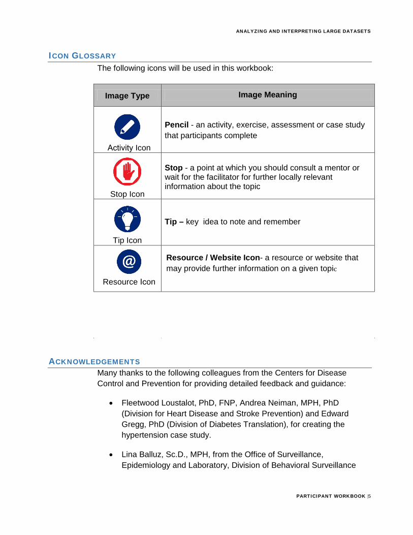
ICON GLOSSARY The following icons will be used in this workbook:
Image Type Image Meaning
Activity Icon
Pencil - an activity, exercise, assessment or case study that participants complete
Stop Icon
Stop - a point at which you should consult a mentor or wait for the facilitator for further locally relevant information about the topic
Tip Icon
Tip – key idea to note and remember
Resource Icon
Resource / Website Icon- a resource or website that may provide further information on a given topic
ACKNOWLEDGEMENTS Many thanks to the following colleagues from the Centers for Disease Control and Prevention for providing detailed feedback and guidance:
• Fleetwood Loustalot, PhD, FNP, Andrea Neiman, MPH, PhD(Division for Heart Disease and Stroke Prevention) and EdwardGregg, PhD (Division of Diabetes Translation), for creating thehypertension case study.
• Lina Balluz, Sc.D., MPH, from the Office of Surveillance,Epidemiology and Laboratory, Division of Behavioral Surveillance

ANALYZING AND INTERPRETING LARGE DATASETS
PARTICIPANT WORKBOOK |6
• Richard Dicker, MD, MS, from the Centers for Global Health, Divisionof Public Health Systems Workforce Development
• Italia Rolle, PhD, RD, Office on Smoking and Health, Global TobaccoControl Branch
• Roberto (Felipe) Lobelo, MD, PhD, Division of Diabetes Translation
ANALYZING AND INTERPRETING LARGE DATASETS
PARTICIPANT WORKBOOK |7
Section 1: Overview
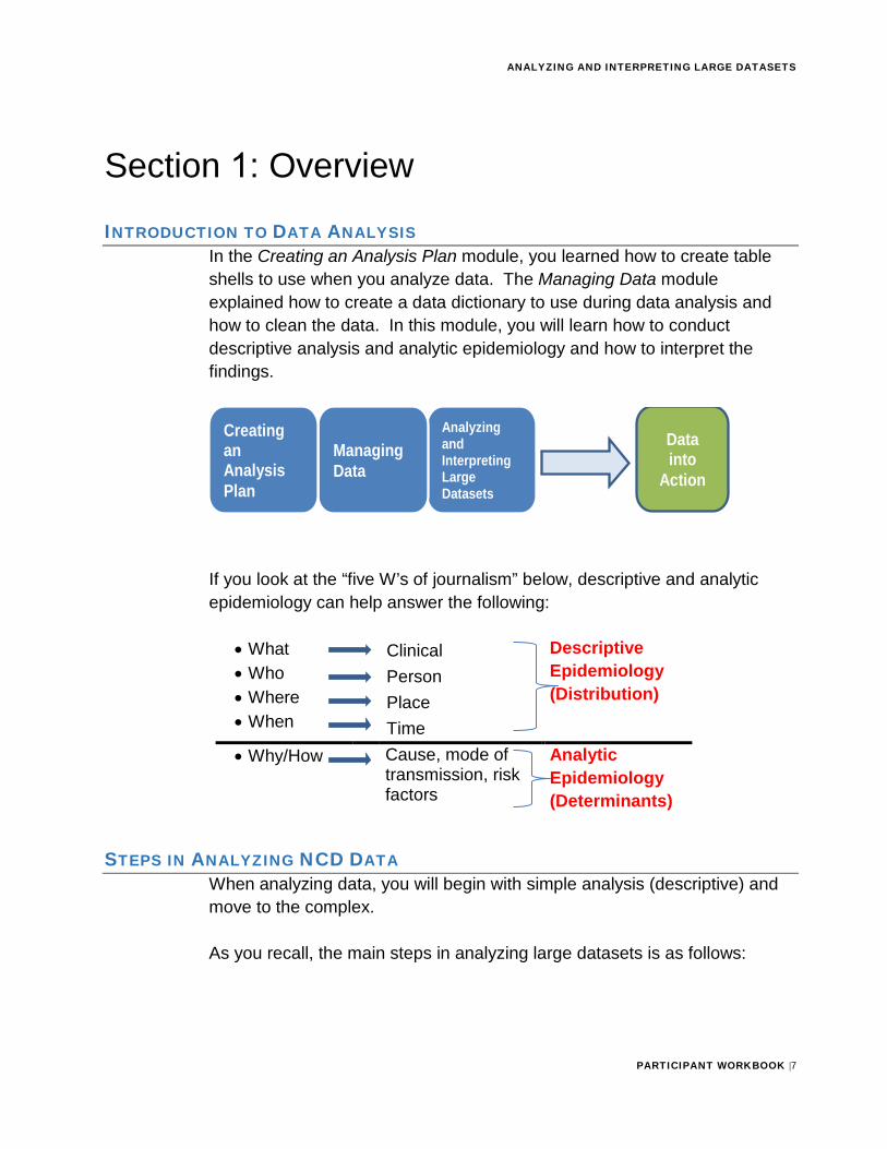
INTRODUCTION TO DATA ANALYSISIn the Creating an Analysis Plan module, you learned how to create table shells to use when you analyze data. The Managing Data module explained how to create a data dictionary to use during data analysis and how to clean the data. In this module, you will learn how to conduct descriptive analysis and analytic epidemiology and how to interpret the findings.
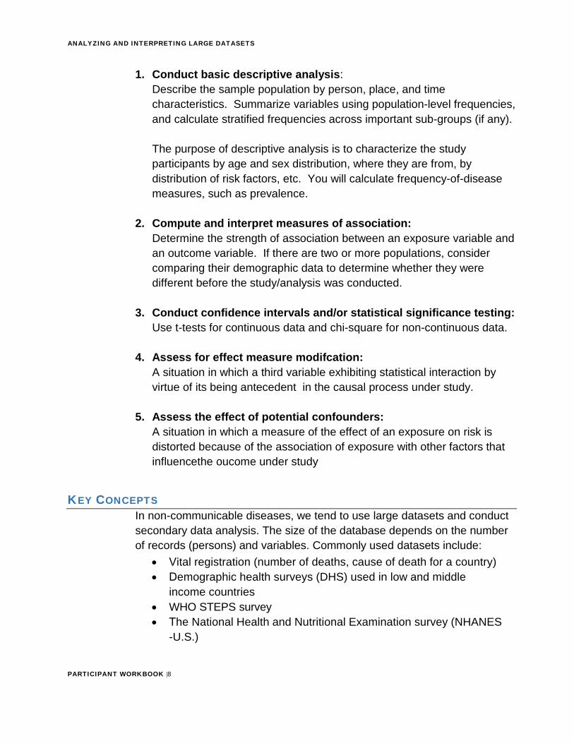
If you look at the “five W’s of journalism” below, descriptive and analytic epidemiology can help answer the following:
• What• Who• Where• When
Clinical Person Place Time
Descriptive Epidemiology (Distribution)
• Why/How Cause, mode of transmission, risk factors
Analytic Epidemiology (Determinants)
STEPS IN ANALYZING NCD DATAWhen analyzing data, you will begin with simple analysis (descriptive) and move to the complex.
As you recall, the main steps in analyzing large datasets is as follows:
Data into
Action
Analyzing and Interpreting Large Datasets
Managing Data
Creating an Analysis Plan
ANALYZING AND INTERPRETING LARGE DATASETS
PARTICIPANT WORKBOOK |8
1. Conduct basic descriptive analysis:Describe the sample population by person, place, and timecharacteristics. Summarize variables using population-level frequencies,and calculate stratified frequencies across important sub-groups (if any).
The purpose of descriptive analysis is to characterize the study participants by age and sex distribution, where they are from, by distribution of risk factors, etc. You will calculate frequency-of-disease measures, such as prevalence.
2. Compute and interpret measures of association:Determine the strength of association between an exposure variable andan outcome variable. If there are two or more populations, considercomparing their demographic data to determine whether they weredifferent before the study/analysis was conducted.
3. Conduct confidence intervals and/or statistical significance testing:Use t-tests for continuous data and chi-square for non-continuous data.
4. Assess for effect measure modifcation:A situation in which a third variable exhibiting statistical interaction byvirtue of its being antecedent in the causal process under study.
5. Assess the effect of potential confounders:A situation in which a measure of the effect of an exposure on risk isdistorted because of the association of exposure with other factors thatinfluencethe oucome under study
KEY CONCEPTSIn non-communicable diseases, we tend to use large datasets and conduct secondary data analysis. The size of the database depends on the number of records (persons) and variables. Commonly used datasets include:
• Vital registration (number of deaths, cause of death for a country)• Demographic health surveys (DHS) used in low and middle
income countries• WHO STEPS survey• The National Health and Nutritional Examination survey (NHANES
-U.S.)
ANALYZING AND INTERPRETING LARGE DATASETS
PARTICIPANT WORKBOOK |9
• The Behavioral Risk Factor Surveillance System (BRFSS - U.S., Jordan)
The databases typically are representative of a population either through a census (all persons included) or a sample (number of people selected to represent the population). For example, NHANES 1999-2000 interviewed 9,965 persons in the United States and the database includes hundreds of variables. Before attempting data analysis for large datasets, it is very important you locate the survey sampling methodology, questionnaire, data variable dictionary and any other supporting documentation.
Activity
Activity #1: Go to the NHANES links below and describe what key information they provide. Write your response in the space below. Then check your response with Appendix A.
1. http://www.cdc.gov/nchs/nhanes/nhanes1999-2000/questexam99_00.htm;
2. http://www.cdc.gov/nchs/data/nhanes/nhanes_03_04/nhanes_analytic_guidelines_dec_2005.pdf
ANALYZING AND INTERPRETING LARGE DATASETS
PARTICIPANT WORKBOOK |10
Once you have your data, determine if the data include: • All persons in the population of interest (census)• A sample representative of the population (e.g. probability simple
random sample, random sample or cluster sampling)• A sample not representative of the population (e.g. non-probability
convenience sampling or purposive sampling)
Knowing this information will inform the statistics you will use during data analysis.
ANALYZING AND INTERPRETING LARGE DATASETS
PARTICIPANT WORKBOOK |11
Survey Commands For samples that are from complex survey designs, you must use the appropriate survey commands and not the regular commands in your statistical survey software.
Before setting these commands, always look at the raw data before applying the survey commands using the non-survey commands. This would be the first step before performing univariable analysis to view the data. In addition, for complex survey designs, you must set the weight command, strata, and psu (primary sampling unit) commands when computing representative estimates of the variables.
After examining the data and finalizing your data analysis plan, proceed with using the survey commands to obtain estimates that account for the complex survey design and weighting. These estimates, although from a sample, are now representative of the population that was sampled.
Population Parameters and Sample Statistics The following table is helpful when we talk about population parameters and sample statistics. The measures you use depend on the type of data you are analyzing.
ANALYZING AND INTERPRETING LARGE DATASETS
PARTICIPANT WORKBOOK |12
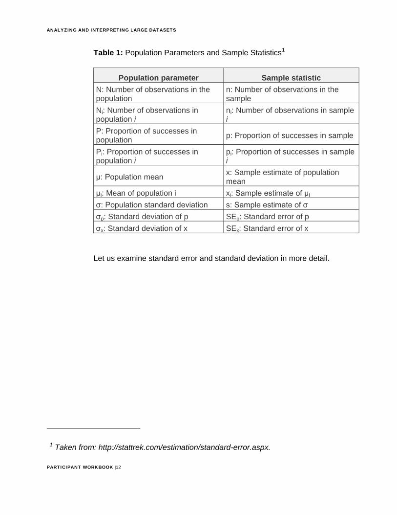
Table 1: Population Parameters and Sample Statistics1
Population parameter Sample statistic N: Number of observations in the population
n: Number of observations in the sample
Ni: Number of observations in population i
ni: Number of observations in sample i
P: Proportion of successes in population p: Proportion of successes in sample
Pi: Proportion of successes in population i
pi: Proportion of successes in sample i
μ: Population mean x: Sample estimate of population mean
μi: Mean of population i xi: Sample estimate of μi σ: Population standard deviation s: Sample estimate of σ σp: Standard deviation of p SEp: Standard error of p σx: Standard deviation of x SEx: Standard error of x
Let us examine standard error and standard deviation in more detail.
1 Taken from: http://stattrek.com/estimation/standard-error.aspx.
ANALYZING AND INTERPRETING LARGE DATASETS
PARTICIPANT WORKBOOK |13
Standard Deviation The standard deviation reflects the variability of the distribution of a continuous variable. To estimate the standard deviation: 1. Calculate the weighted sum of the squares of the differences of the
observations in a simple random sample from the sample mean
2. Divide the result obtained in #1 by an estimate of the population size minus 1
3. Take the square root of the result obtained in #2
Standard Error of the Mean The standard error of the mean is an indication of how well the mean of a sample estimates the mean of a population. To estimate the standard error, divide the estimated standard deviation by the square root of the sample size.
Application of Weights In addition to population parameters and survey statistics, another important concept you need to know when using complex survey data is the use of weights.
Use weights to account for complex survey design (including oversampling), survey non-response, and post-stratification. When a sample is weighted, it is representative of the population. A sample weight is assigned to each sample person. It is a measure of the number of people in the population represented by that sample person. Fortunately, there are several software packages for survey analysis that compute sampling errors correctly for weighted survey estimates from complex sample designs.
It is important to use weighted data when you need to generalize the findings from your study to the whole population. . Weighting is a technique usually done by statistician to assure representation of cetain groups in the sample. It is a process that removes non-response and non -coverage bias.
Resource
For an example of standard error: http://www.bmj.com/content/343/bmj.d8010
ANALYZING AND INTERPRETING LARGE DATASETS
PARTICIPANT WORKBOOK |14
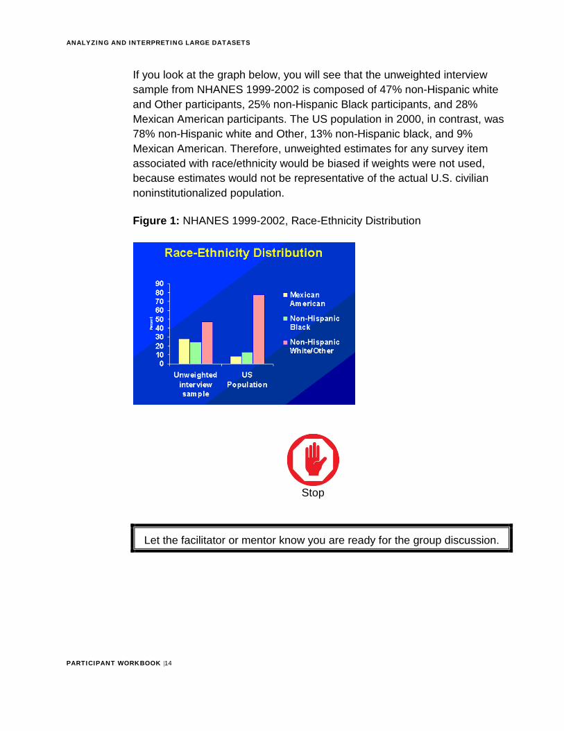
If you look at the graph below, you will see that the unweighted interview sample from NHANES 1999-2002 is composed of 47% non-Hispanic white and Other participants, 25% non-Hispanic Black participants, and 28% Mexican American participants. The US population in 2000, in contrast, was 78% non-Hispanic white and Other, 13% non-Hispanic black, and 9% Mexican American. Therefore, unweighted estimates for any survey item associated with race/ethnicity would be biased if weights were not used, because estimates would not be representative of the actual U.S. civilian noninstitutionalized population.
Figure 1: NHANES 1999-2002, Race-Ethnicity Distribution
Stop
Let the facilitator or mentor know you are ready for the group discussion.
ANALYZING AND INTERPRETING LARGE DATASETS
PARTICIPANT WORKBOOK |15
Section 2: Descriptive Analysis
OVERVIEW OF DESCRIPTIVE ANALYSISDescriptive analysis involves computing frequency distributions (also known as univariable analysis) and simple cross-tabulations (bivariable analysis). This helps you characterize the population under study and understand the occurrence of outcomes and exposures by person, place, and time characteristics.
The objectives of descriptive analysis are to: • Describe and assess the health status of a population• Evaluate patterns of disease and allow comparisons over time and place• Provide a basis for planning and evaluation of services• Identify problems to be studied by analytic methods, including testing
hypotheses related to those problems
Conducting univariable data analysis involves analyzing one variable at a time in a dataset, such as sex, age, or education. You can assess the range, mean, median and mode of each continuous variable and the range and frequency distribution of discrete variables. You will then examine the prevalence by demographics (e.g., age, marital status, location).
Conducting bivariable analysis involves analyzing the relationship between two variables. You will compare the outcome populations of interest in terms of demographic characteristics (e.g., comparing differences in age, gender, ethnicity, income, or location between cases and controls).
Depending on the questions you need answered, descriptive analysis can reveal information related to the factors of person, place, and time in the population of interest such as:
• The characteristics of the population, such as age, gender,where they live (e.g., urban or rural)
• The prevalence of the population affected by the disease,outcomes, or exposures
• The prevalence of risk factors among the population• When the events of interest occurred, such as monthly or yearly
ANALYZING AND INTERPRETING LARGE DATASETS
PARTICIPANT WORKBOOK |16
Tip
Remember to use the table shells you created in your analysis plan when describing the characteristics from descriptive analysis.
For this section of the module, you will practice conducting descriptive analysis for the hypertension case study and your own country data.
UNIVARIABLE ANALYSISWhen you cleaned your dataset, you looked at key descriptive variables (such as age, sex, marital status, education level, and occupation). Now you will examine the results and organize them into tables and graphs so that you can compare the variables.
Run Frequencies A frequency distribution shows the number of observations located in each category of a categorical variable (e.g., sex, level of education, marital status). For continuous variables, such as age, frequencies are displayed for values that appear at least one time in the dataset.
Frequency distributions provide an organized picture of the data, and allow you to see how individual scores are distributed on a specified scale of measurement. For instance, a frequency distribution shows whether the data values are generally high or low, and whether they are concentrated in one area or spread out across the entire measurement scale.
You can structure frequency distributions as tables or graphs, but either should show the original measurement scale and the frequencies associated with each category. Datasets with very large sample sizes can potentially have a long list of different values for continuous variables; therefore, it is recommended that you use a graphic format to check the distribution for continuous variables, and either frequency tables or graphic forms for nominal or interval variables.
ANALYZING AND INTERPRETING LARGE DATASETS
PARTICIPANT WORKBOOK |17
For large datasets, analyze continuous variables (such as age) by determining the mean, median, standard deviation and interquartile range (IQR). Analyze nominal variables (such as gender) by using percentages.
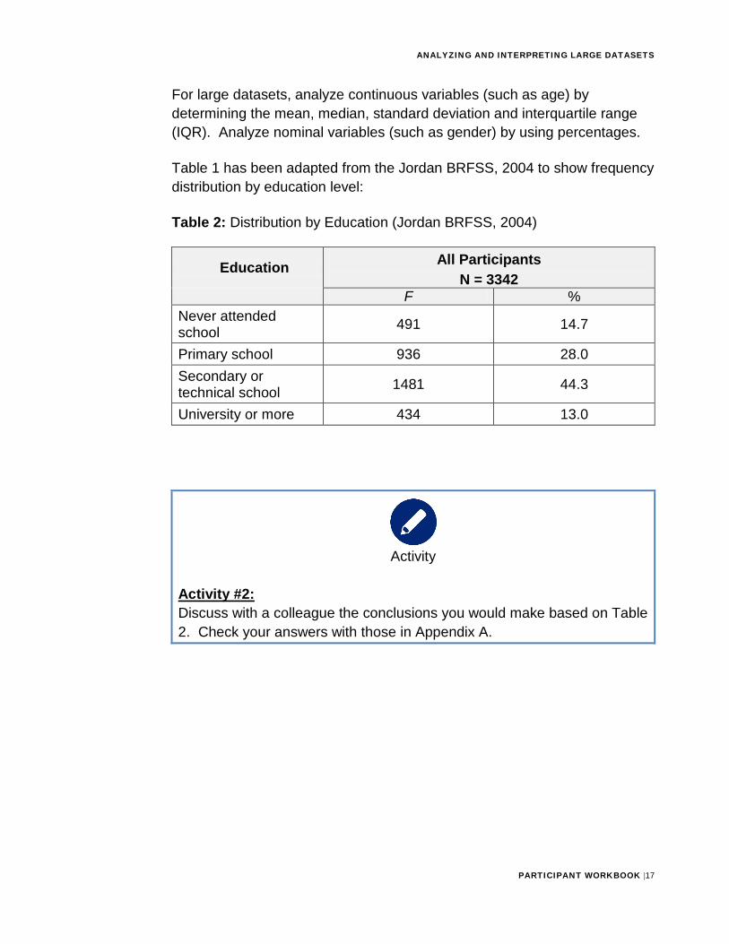
Table 1 has been adapted from the Jordan BRFSS, 2004 to show frequency distribution by education level:
Table 2: Distribution by Education (Jordan BRFSS, 2004)
Education All Participants N = 3342
F % Never attended school 491 14.7
Primary school 936 28.0 Secondary or technical school 1481 44.3
University or more 434 13.0
Activity
Activity #2: Discuss with a colleague the conclusions you would make based on Table 2. Check your answers with those in Appendix A.
ANALYZING AND INTERPRETING LARGE DATASETS
PARTICIPANT WORKBOOK |18
Creating Intervals or Categories The mean and median of continuous variables provide useful information; however, there are times when you may want to group the continuous variable data into logical intervals or categories. You will then compare the frequency distributions of the new categories.
Consider these guidelines when creating intervals: • Create intervals that are mutually exclusive and include all of the
data• Use a relatively large number of narrow intervals initially. You can
combine intervals again after you look carefully at the distributions.• Use natural or biologically meaningful intervals when possible. For
example, look at standard or frequently used age groupings whenconsidering age.
• Create a category for unknowns if relevant
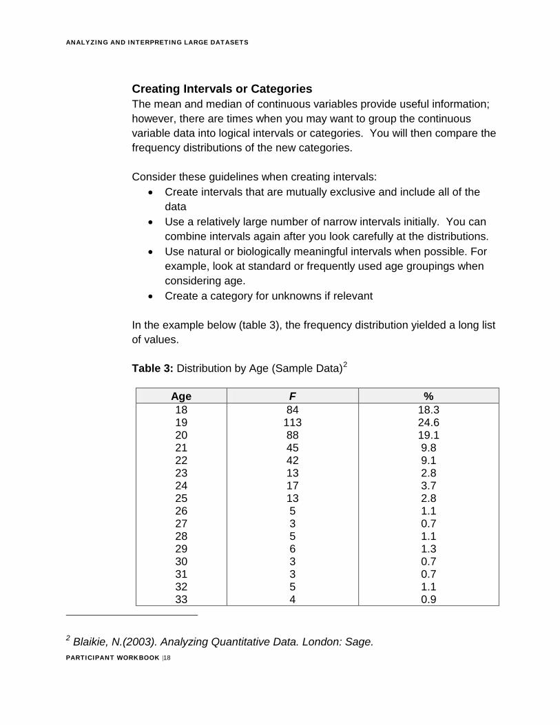
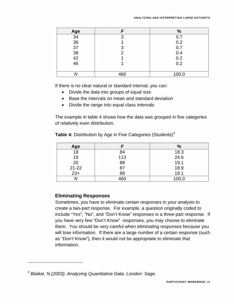
In the example below (table 3), the frequency distribution yielded a long list of values.
Table 3: Distribution by Age (Sample Data)2
Age F % 18 19 20 21 22 23 24 25 26 27 28 29 30 31 32 33
84 113 88 45 42 13 17 13 53563354
18.3 24.6 19.1 9.8 9.1 2.8 3.7 2.8 1.1 0.7 1.1 1.3 0.7 0.7 1.1 0.9
2 Blaikie, N.(2003). Analyzing Quantitative Data. London: Sage.
ANALYZING AND INTERPRETING LARGE DATASETS
PARTICIPANT WORKBOOK |19
Age F % 34 36 37 38 42 46
313211
0.7 0.2 0.7 0.4 0.2 0.2
N 460 100.0
If there is no clear natural or standard interval, you can: • Divide the data into groups of equal size• Base the intervals on mean and standard deviation• Divide the range into equal class intervals
The example in table 4 shows how the data was grouped in five categories of relatively even distribution.
Table 4: Distribution by Age in Five Categories (Students)3
Age F % 18 19 20
21-22 23+
84 113 88 87 88
18.3 24.6 19.1 18.9 19.1
N 460 100.0
Eliminating Responses Sometimes, you have to eliminate certain responses in your analysis to create a two-part response. For example, a question originally coded to include “Yes”, “No”, and “Don’t Know” responses is a three-part response. If you have very few “Don’t Know” responses, you may choose to eliminate them. You should be very careful when eliminating responses because you will lose information. If there are a large number of a certain response (such as “Don’t Know”), then it would not be appropriate to eliminate that information.
3 Blaikie, N.(2003). Analyzing Quantitative Data. London: Sage.
ANALYZING AND INTERPRETING LARGE DATASETS
PARTICIPANT WORKBOOK |20
Tip
If there is only a very small number of responses, then eliminating the information can be an appropriate choice to improve your interpretation
of the variable.
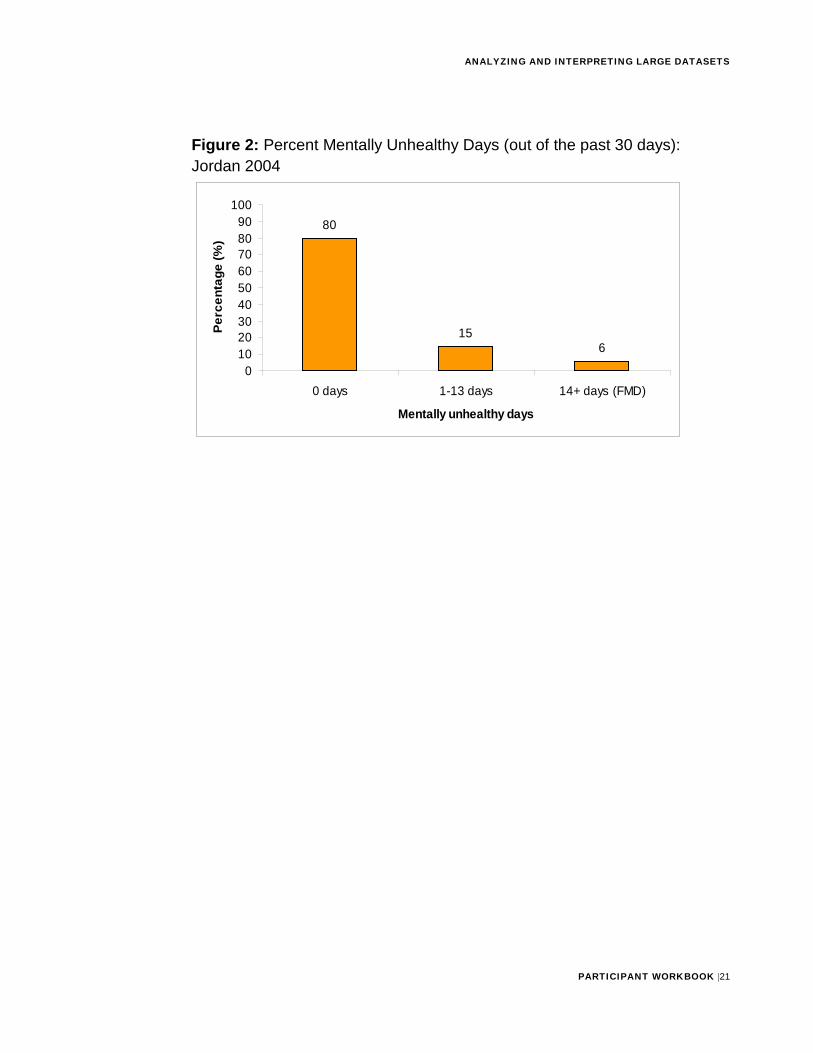
Prevalence Recall that prevalence is a proportion that expresses the presence of a disease or other characteristic at a specific point in time. To calculate the prevalence of a disease or other health outcome, divide the number of cases in a population at a specific time by the total population at that period of time. Similarly, to calculate the prevalence of a risk factor such as smoking or other characteristic, divide the number of people with that risk factor at a specific time by the total population at that period of time.
For example, one of the research questions for the 2004 Jordan Behavioral Risk Factor Survey was: To determine prevalence of frequent mental distress (FMD) (a proxy for mental illness), using number of mentally unhealthy days among adult Jordanians.
• Health Related Quality of Life question:“Now thinking about your mental health, which includes stress,depression, and problems with emotions, for how many days duringthe past 30 days was your mental health not good?”
• Frequent Mental Distress was defined as >14 days of mental healthnot good.
Activity
Activity #3: Discuss with a colleague the conclusions you would make based on Figure 2 below. Then check your responses with those in Appendix A.
ANALYZING AND INTERPRETING LARGE DATASETS
PARTICIPANT WORKBOOK |21
Figure 2: Percent Mentally Unhealthy Days (out of the past 30 days): Jordan 2004
80
156
0102030405060708090
100
0 days 1-13 days 14+ days (FMD)
Mentally unhealthy days
Perc
enta
ge (%
)
ANALYZING AND INTERPRETING LARGE DATASETS
PARTICIPANT WORKBOOK |22
To analyze the data by certain demographics, such as age, education and income, you will conduct bivariable analysis (discussed in the next section).
Stop
Let the facilitator or mentor know you are ready for a group discussion. He or she will review key concepts of conducting univariable analysis
before you complete Exercise 1.
KEY POINTS TO REMEMBERUse the space below to record any key points from the facilitator-led discussion:
Practice Exercise #1 (Estimated time: 1 hour)
Background: For this exercise, you will work individually, in pairs or in a small group to compute univariable analysis.
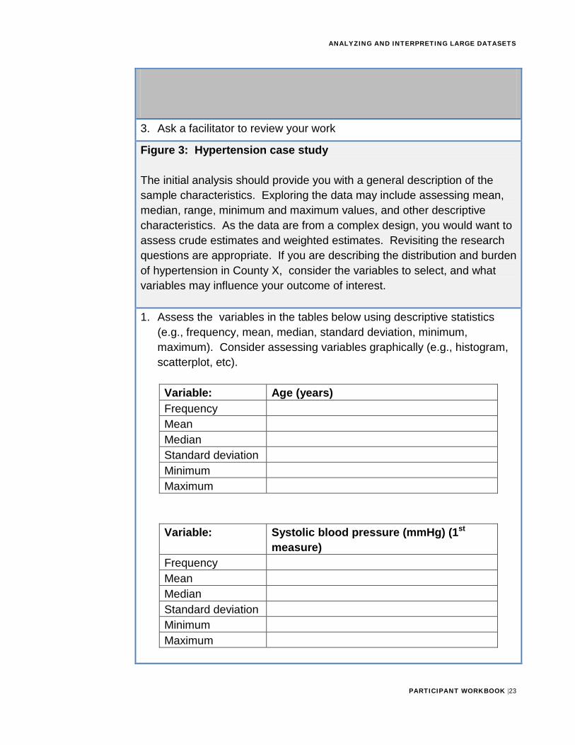
Instructions: 1. Read figure 3
2. Answer the questions that follow
ANALYZING AND INTERPRETING LARGE DATASETS
PARTICIPANT WORKBOOK |23
3. Ask a facilitator to review your work
Figure 3: Hypertension case study
The initial analysis should provide you with a general description of the sample characteristics. Exploring the data may include assessing mean, median, range, minimum and maximum values, and other descriptive characteristics. As the data are from a complex design, you would want to assess crude estimates and weighted estimates. Revisiting the research questions are appropriate. If you are describing the distribution and burden of hypertension in County X, consider the variables to select, and what variables may influence your outcome of interest.
1. Assess the variables in the tables below using descriptive statistics(e.g., frequency, mean, median, standard deviation, minimum,maximum). Consider assessing variables graphically (e.g., histogram,scatterplot, etc).
Variable: Age (years) Frequency Mean Median Standard deviation Minimum Maximum
Variable: Systolic blood pressure (mmHg) (1st measure)
Frequency Mean Median Standard deviation Minimum Maximum
ANALYZING AND INTERPRETING LARGE DATASETS
PARTICIPANT WORKBOOK |24
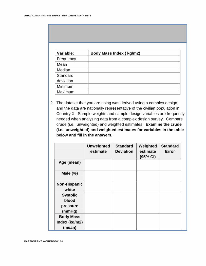
Variable: Body Mass Index ( kg/m2) Frequency Mean Median Standard deviation Minimum Maximum
2. The dataset that you are using was derived using a complex design,and the data are nationally representative of the civilian population inCountry X. Sample weights and sample design variables are frequentlyneeded when analyzing data from a complex design survey. Comparecrude (i.e., unweighted) and weighted estimates. Examine the crude(i.e., unweighted) and weighted estimates for variables in the tablebelow and fill in the answers.
Unweighted estimate
Standard Deviation
Weighted estimate (95% CI)
Standard Error
Age (mean)
Male (%)
Non-Hispanic white
Systolic blood
pressure (mmHg)
Body Mass Index (kg/m2)
(mean)
ANALYZING AND INTERPRETING LARGE DATASETS
PARTICIPANT WORKBOOK |25
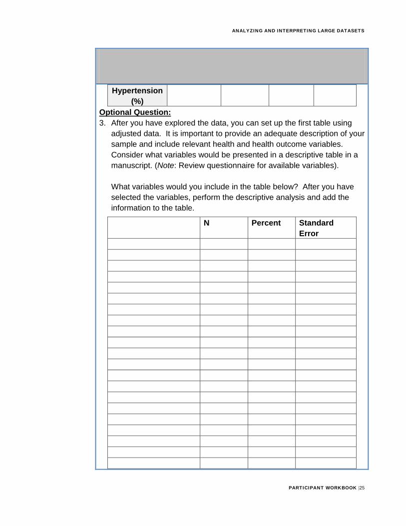
Hypertension (%)
Optional Question: 3. After you have explored the data, you can set up the first table using
adjusted data. It is important to provide an adequate description of yoursample and include relevant health and health outcome variables.Consider what variables would be presented in a descriptive table in amanuscript. (Note: Review questionnaire for available variables).
What variables would you include in the table below? After you have selected the variables, perform the descriptive analysis and add the information to the table.
N Percent Standard Error
ANALYZING AND INTERPRETING LARGE DATASETS
PARTICIPANT WORKBOOK |26
BIVARIABLE ANALYSISAs you recall, bivariable analysis involves either:
• Establishing similarities or differences of the demographic characteristics (e.g., age, gender, ethnicity, income, or location) and/or exposure characteristics (e.g., drug use, environmental exposure, diet, exposure to other ill persons, family history of disease)
• Describing patterns or connections between such characteristics
Simple Cross-Tabulations A cross-tabulation (cross-tab) is a two or more dimensional table that records the number (frequency) of respondents that have the specific characteristics described in the cells of the table. You can use cross-tabs to visually assess whether independent and dependent variables might be related. You can also use cross-tabs to find out if demographic variables such as sex and age are related to the second variable.
Use cross-tabs when you want:
• To look at relationships among two or three variables
• A descriptive statistical measure to determine whether differences among groups are large enough to indicate some sort of relationship among variables
Refer to an example of cross-tabs in Table 5 below.
ANALYZING AND INTERPRETING LARGE DATASETS
PARTICIPANT WORKBOOK |27
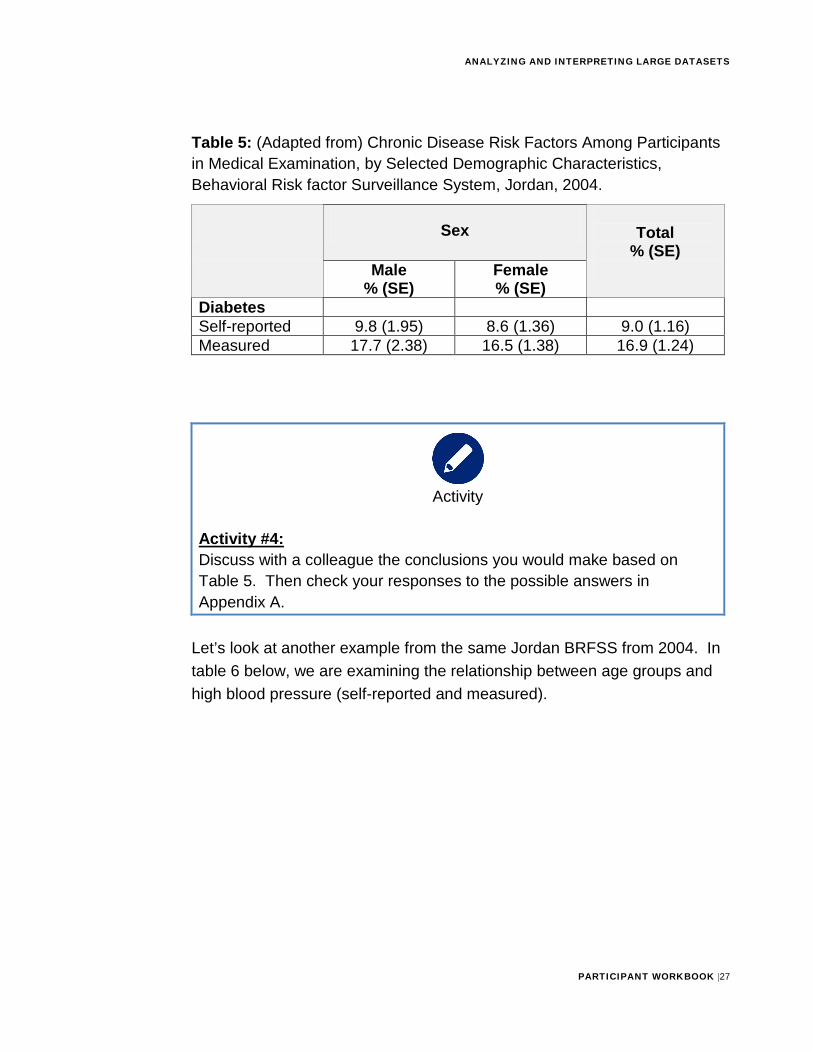
Table 5: (Adapted from) Chronic Disease Risk Factors Among Participants in Medical Examination, by Selected Demographic Characteristics, Behavioral Risk factor Surveillance System, Jordan, 2004.
Sex Total % (SE)
Male % (SE)
Female % (SE)
Diabetes Self-reported 9.8 (1.95) 8.6 (1.36) 9.0 (1.16) Measured 17.7 (2.38) 16.5 (1.38) 16.9 (1.24)
Activity
Activity #4: Discuss with a colleague the conclusions you would make based on Table 5. Then check your responses to the possible answers in Appendix A.
Let’s look at another example from the same Jordan BRFSS from 2004. In table 6 below, we are examining the relationship between age groups and high blood pressure (self-reported and measured).
ANALYZING AND INTERPRETING LARGE DATASETS
PARTICIPANT WORKBOOK |28
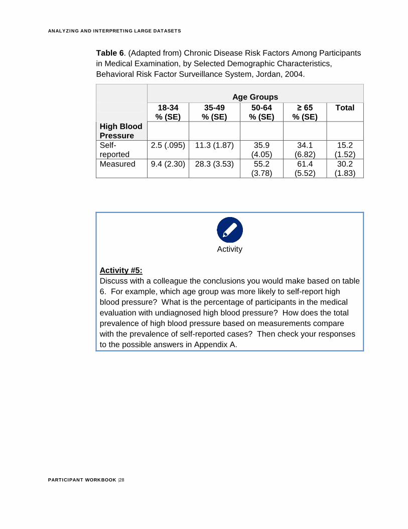
Table 6. (Adapted from) Chronic Disease Risk Factors Among Participants in Medical Examination, by Selected Demographic Characteristics, Behavioral Risk Factor Surveillance System, Jordan, 2004.
Age Groups 18-34
% (SE) 35-49
% (SE) 50-64
% (SE) ≥ 65
% (SE) Total
High Blood Pressure Self-reported
2.5 (.095) 11.3 (1.87) 35.9 (4.05)
34.1 (6.82)
15.2 (1.52)
Measured 9.4 (2.30) 28.3 (3.53) 55.2 (3.78)
61.4 (5.52)
30.2 (1.83)
Activity
Activity #5: Discuss with a colleague the conclusions you would make based on table 6. For example, which age group was more likely to self-report highblood pressure? What is the percentage of participants in the medical evaluation with undiagnosed high blood pressure? How does the total prevalence of high blood pressure based on measurements compare with the prevalence of self-reported cases? Then check your responses to the possible answers in Appendix A.
ANALYZING AND INTERPRETING LARGE DATASETS
PARTICIPANT WORKBOOK |29
Tip
Cross tabs are not sufficient to: • Show the strength or actual size of the relationship among two
or more variables • Test a hypothesis about the relationship between two or more
variablesInstead, use analytic epidemiology (explained in the section 4).
Analyzing Demographic Characteristics Using bivariable analysis allows you to detect similarities or differences of the demographic characteristics (e.g., age, gender, ethnicity, income, or location).
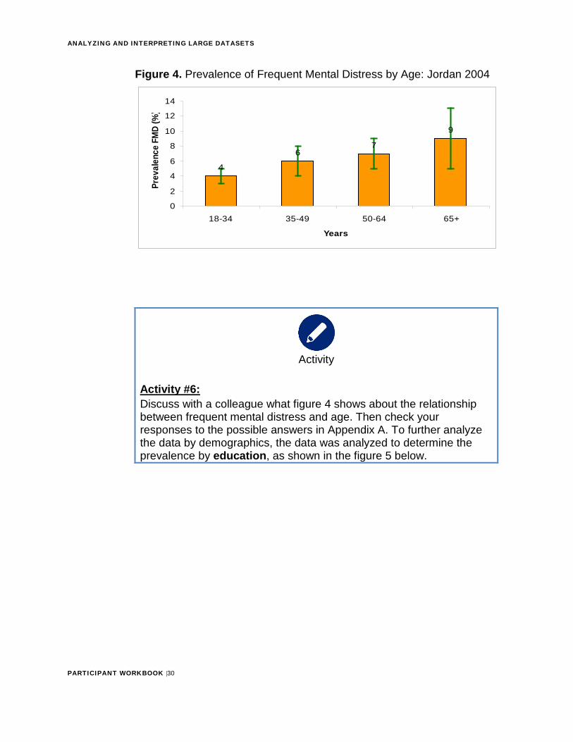
In the Jordan study of the prevalence of frequent mental distress, it was found that 6% of Jordanian adults would be classified as experiencing frequent mental distress. The next few graphs show the prevalence of frequent mental distress by age, education, and income.
ANALYZING AND INTERPRETING LARGE DATASETS
PARTICIPANT WORKBOOK |30
Figure 4. Prevalence of Frequent Mental Distress by Age: Jordan 2004
Activity
Activity #6: Discuss with a colleague what figure 4 shows about the relationship between frequent mental distress and age. Then check your responses to the possible answers in Appendix A. To further analyze the data by demographics, the data was analyzed to determine the prevalence by education, as shown in the figure 5 below.
4
67
9
0
2
4
6
8
10
12
14
18-34 35-49 50-64 65+
Years
Prev
alen
ce F
MD
(%)
ANALYZING AND INTERPRETING LARGE DATASETS
PARTICIPANT WORKBOOK |31
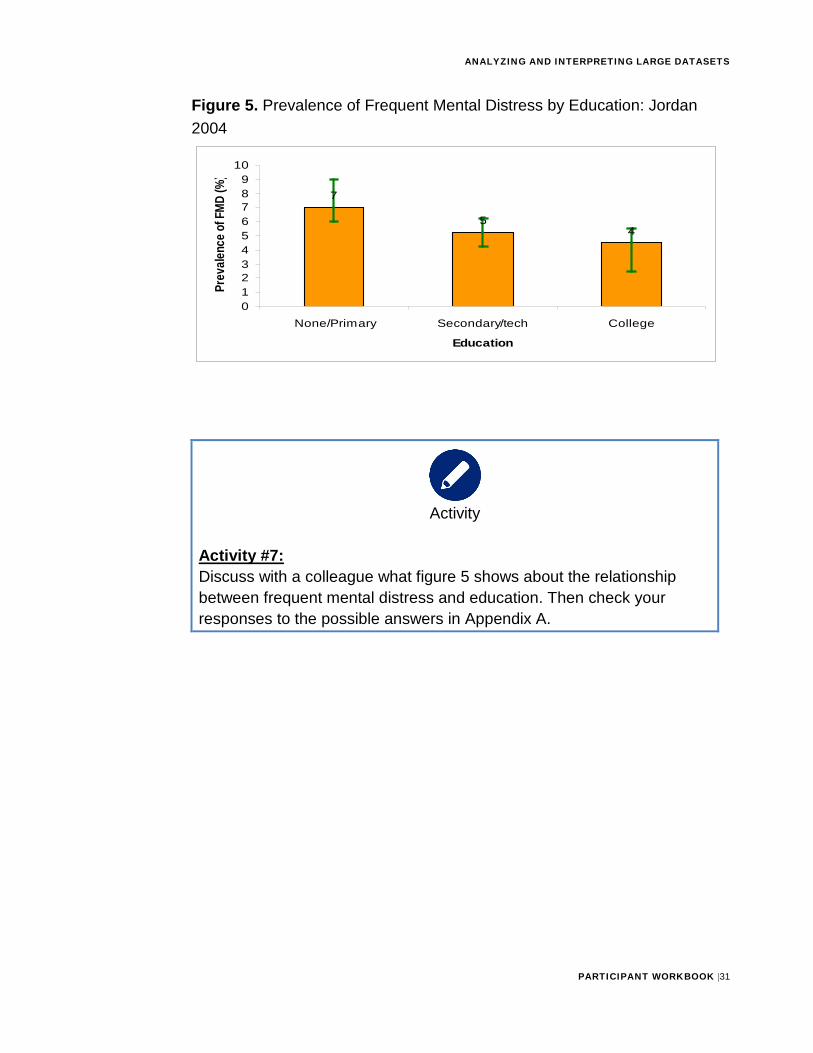
Figure 5. Prevalence of Frequent Mental Distress by Education: Jordan 2004
Activity
Activity #7: Discuss with a colleague what figure 5 shows about the relationship between frequent mental distress and education. Then check your responses to the possible answers in Appendix A.
7
54
0123456789
10
None/Primary Secondary/tech College
Education
Prev
alenc
e of F
MD (%
)
ANALYZING AND INTERPRETING LARGE DATASETS
PARTICIPANT WORKBOOK |32
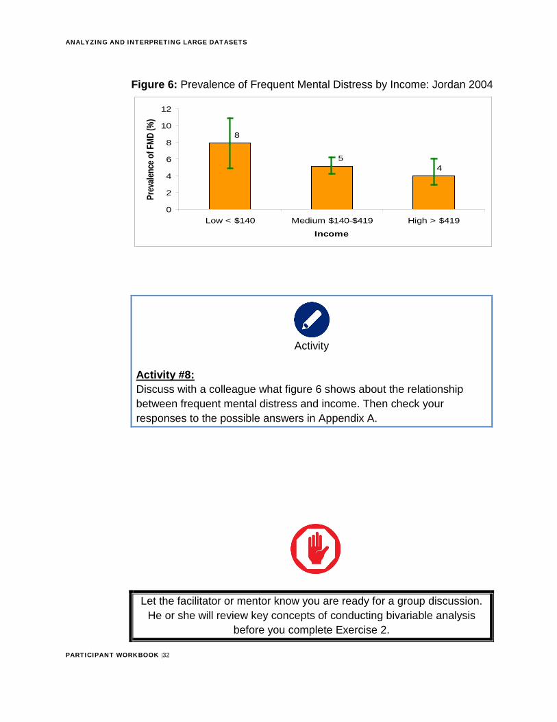
Figure 6: Prevalence of Frequent Mental Distress by Income: Jordan 2004
Activity
Activity #8: Discuss with a colleague what figure 6 shows about the relationship between frequent mental distress and income. Then check your responses to the possible answers in Appendix A.
Let the facilitator or mentor know you are ready for a group discussion. He or she will review key concepts of conducting bivariable analysis
before you complete Exercise 2.
45
8
0
2
4
6
8
10
12
Low < $140 Medium $140-$419 High > $419
Income
Prev
alenc
e of F
MD (%
)
ANALYZING AND INTERPRETING LARGE DATASETS
PARTICIPANT WORKBOOK |33
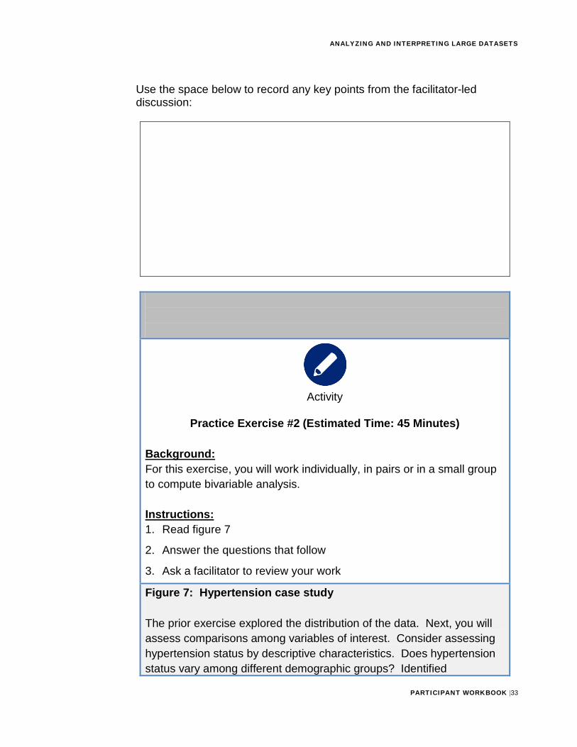
Use the space below to record any key points from the facilitator-led discussion:
Activity
Practice Exercise #2 (Estimated Time: 45 Minutes)
Background: For this exercise, you will work individually, in pairs or in a small group to compute bivariable analysis.
Instructions: 1. Read figure 7
2. Answer the questions that follow
3. Ask a facilitator to review your work
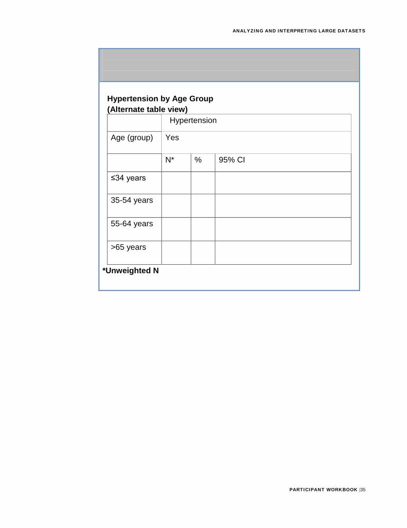
Figure 7: Hypertension case study
The prior exercise explored the distribution of the data. Next, you will assess comparisons among variables of interest. Consider assessing hypertension status by descriptive characteristics. Does hypertension status vary among different demographic groups? Identified
ANALYZING AND INTERPRETING LARGE DATASETS
PARTICIPANT WORKBOOK |34
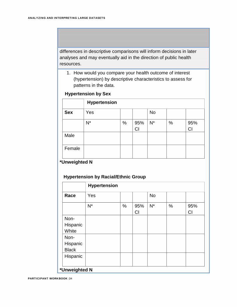
differences in descriptive comparisons will inform decisions in later analyses and may eventually aid in the direction of public health resources.
1. How would you compare your health outcome of interest(hypertension) by descriptive characteristics to assess forpatterns in the data.
Hypertension by Sex
Hypertension
Sex Yes No
N* % 95% CI
N* % 95% CI
Male
Female
*Unweighted N
Hypertension by Racial/Ethnic Group
Hypertension
Race Yes No
N* % 95% CI
N* % 95% CI
Non-Hispanic White Non-Hispanic Black Hispanic
*Unweighted N
ANALYZING AND INTERPRETING LARGE DATASETS
PARTICIPANT WORKBOOK |35
Hypertension by Age Group (Alternate table view)
Hypertension
Age (group) Yes
N* % 95% CI
≤34 years
35-54 years
55-64 years
>65 years
*Unweighted N
ANALYZING AND INTERPRETING LARGE DATASETS
PARTICIPANT WORKBOOK |36
Section 3: Analytic Epidemiology OVERVIEW
In the last section, you learned that one primary purpose of conducting descriptive analysis is to generate hypotheses by revealing the burden and distribution of health events by person, place and time. In contrast, you will conduct analytic epidemiology to test hypotheses by quantifying the strength of association between a suspected risk factor and the health event.
CONCEPTS OF ASSOCIATIONA measure of association quantifies the degree of statistical connection between two variables (the “exposure” and the outcome). In this context, “exposure” refers to an external exposure such as radiation or medication, and also behavior, genetic make-up or any other characteristic of a person. In this section, we assume that the health outcome of interest is measured as a binary variable, i.e., present or absent.
When we measure the health outcome in terms of incidence (new cases), measures of association in epidemiology include the risk ratio4, rate ratio5, odds ratio (OR), risk difference, and rate difference. You should already be familiar with these measures of association and their applications from your introductory epidemiology courses. You can use these measures to evaluate associations between exposures and non-communicable health outcomes for which incidence can be measured, such as acute myocardial infarction.
For many chronic diseases, date of onset is unknown and burden of disease is important. Therefore, you are more likely to measure prevalence rather than incidence. If you measure the outcome in terms of prevalence, the corresponding measures of association are the prevalence ratio and the prevalence odds ratio.
4 Risk ratio is also known as the relative risk or cumulative incidence ratio. 5 Rate ratio is also known as incidence density ratio
ANALYZING AND INTERPRETING LARGE DATASETS
PARTICIPANT WORKBOOK |37
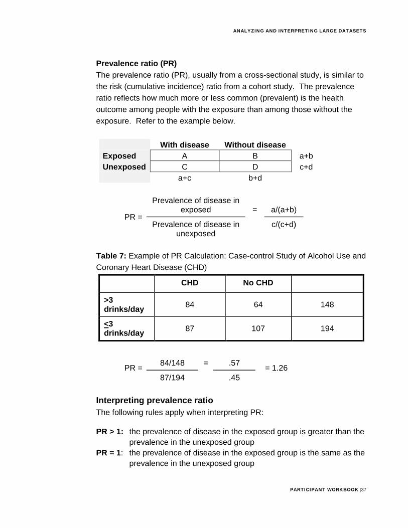
Prevalence ratio (PR) The prevalence ratio (PR), usually from a cross-sectional study, is similar to the risk (cumulative incidence) ratio from a cohort study. The prevalence ratio reflects how much more or less common (prevalent) is the health outcome among people with the exposure than among those without the exposure. Refer to the example below.
With disease Without disease Exposed A B a+b Unexposed C D c+d
a+c b+d
PR =
Prevalence of disease in exposed = a/(a+b)
Prevalence of disease in unexposed
c/(c+d)
Table 7: Example of PR Calculation: Case-control Study of Alcohol Use and Coronary Heart Disease (CHD)
CHD No CHD
>3 drinks/day 84 64 148
<3 drinks/day 87 107 194
PR = 84/148 = .57 = 1.26 87/194 .45
Interpreting prevalence ratio The following rules apply when interpreting PR:
PR > 1: the prevalence of disease in the exposed group is greater than the prevalence in the unexposed group
PR = 1: the prevalence of disease in the exposed group is the same as the prevalence in the unexposed group
ANALYZING AND INTERPRETING LARGE DATASETS
PARTICIPANT WORKBOOK |38
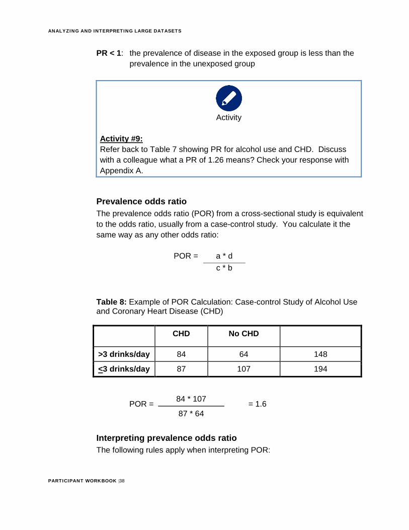
PR < 1: the prevalence of disease in the exposed group is less than the prevalence in the unexposed group
Activity
Activity #9: Refer back to Table 7 showing PR for alcohol use and CHD. Discuss with a colleague what a PR of 1.26 means? Check your response with Appendix A.
Prevalence odds ratio The prevalence odds ratio (POR) from a cross-sectional study is equivalent to the odds ratio, usually from a case-control study. You calculate it the same way as any other odds ratio:
POR = a * d c * b
Table 8: Example of POR Calculation: Case-control Study of Alcohol Use and Coronary Heart Disease (CHD)
CHD No CHD
>3 drinks/day 84 64 148
<3 drinks/day 87 107 194
POR = 84 * 107 = 1.6 87 * 64
Interpreting prevalence odds ratio The following rules apply when interpreting POR:
ANALYZING AND INTERPRETING LARGE DATASETS
PARTICIPANT WORKBOOK |39
POR > 1: the odds of disease in the exposed group is greater than the odds in the unexposed group POR = 1: the odds of disease is the same in the exposed and unexposed (no association) POR < 1: the odds of disease in the exposed group is less than the odds in the unexposed
Activity
Activity #10: Refer to Table 8 above. Discuss with a colleague what a POR of 1.6 means? Check your response with Appendix A.
Using PR or POR For acute disease studies, PR is the preferred measure of association. for cross-sectional studies, POR is the preferred measure of association. Cross-sectional studies are useful for investigating chronic diseases (such as lung cancer) where the onset of disease is difficult to determine. They are also useful for studying long lasting risk factors (such as smoking).
Tip
If the prevalence of the outcome is rare (less than 10%), then the prevalence ratio and the prevalence odds ratio will be approximately equal.
(PR≈POR) Thus, for rare diseases, it does not matter which measure you use.
ANALYZING AND INTERPRETING LARGE DATASETS
PARTICIPANT WORKBOOK |40
Stop
Let the facilitator or mentor know you are ready for a group discussion. He or she will review key concepts of computing and interpreting PR and POR
before you complete Exercise 3.
KEY POINTS TO REMEMBERUse the space below to record any key points from the facilitator-led discussion:
Activity
ANALYZING AND INTERPRETING LARGE DATASETS
PARTICIPANT WORKBOOK |41
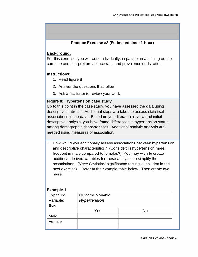
Practice Exercise #3 (Estimated time: 1 hour)
Background: For this exercise, you will work individually, in pairs or in a small group to compute and interpret prevalence ratio and prevalence odds ratio.
Instructions: 1. Read figure 8
2. Answer the questions that follow
3. Ask a facilitator to review your work
Figure 8: Hypertension case study Up to this point in the case study, you have assessed the data using descriptive statistics. Additional steps are taken to assess statistical associations in the data. Based on your literature review and initial descriptive analysis, you have found differences in hypertension status among demographic characteristics. Additional analytic analysis are needed using measures of association.
1. How would you additionally assess associations between hypertensionand descriptive characteristics? (Consider: Is hypertension morefrequent in male compared to females?) You may wish to createadditional derived variables for these analyses to simplify theassociations. (Note: Statistical significance testing is included in thenext exercise). Refer to the example table below. Then create twomore.
Example 1 Exposure Variable: Sex
Outcome Variable: Hypertension
Yes No Male Female
ANALYZING AND INTERPRETING LARGE DATASETS
PARTICIPANT WORKBOOK |42
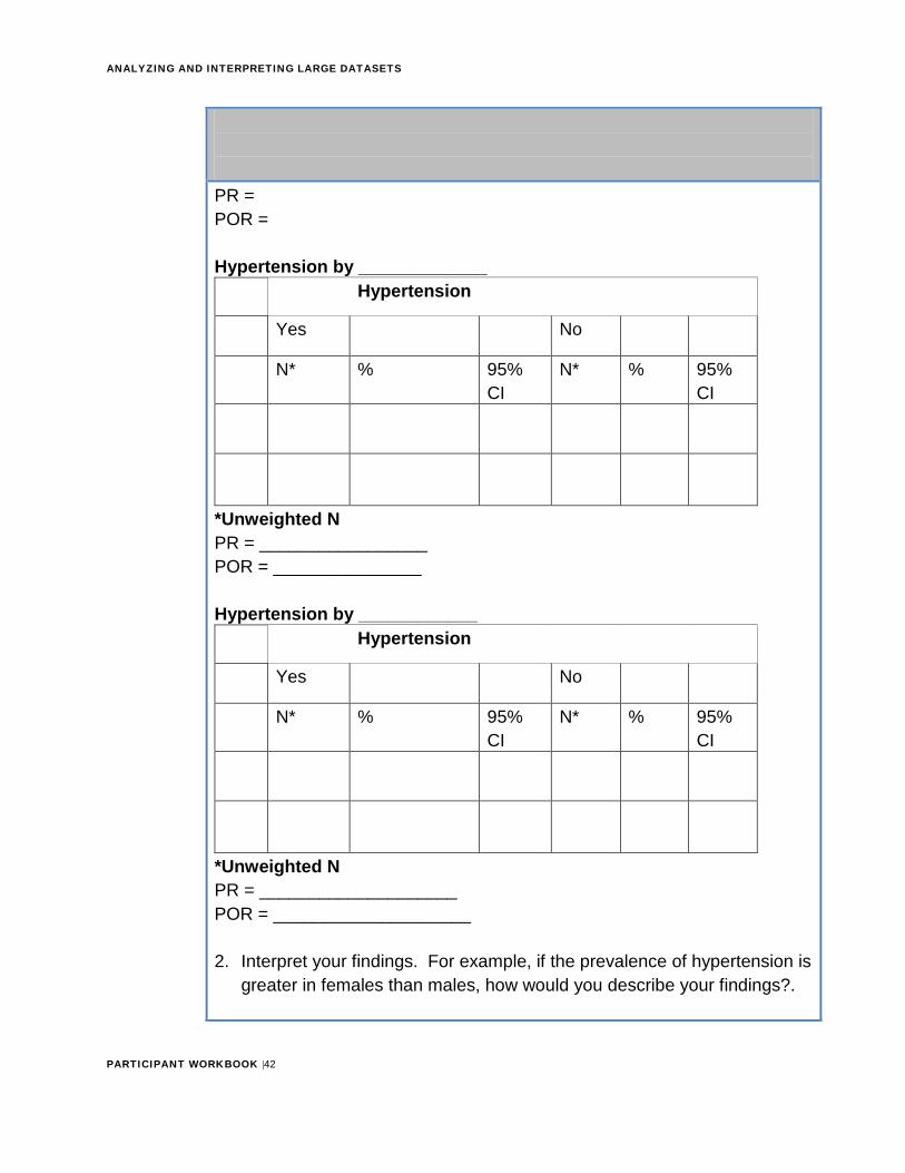
PR = POR =
Hypertension by _____________ Hypertension
Yes No
N* % 95% CI
N* % 95% CI
*Unweighted NPR = _________________ POR = _______________
Hypertension by ____________ Hypertension
Yes No
N* % 95% CI
N* % 95% CI
*Unweighted NPR = ____________________ POR = ____________________
2. Interpret your findings. For example, if the prevalence of hypertension isgreater in females than males, how would you describe your findings?.
ANALYZING AND INTERPRETING LARGE DATASETS
PARTICIPANT WORKBOOK |43
Interpretation:
STATISTICAL SIGNIFICANCE TESTINGYou have calculated an appropriate measure of association from your study, such as the POR = 1.6 for alcohol consumption and CHD. Now you will consider the possibility that the POR in the population is actually 1.0, and the POR of 1.6 calculated from a small sample of that population is simply the result of chance. Statistical significance testing is the process of evaluating whether chance is a reasonable explanation for the observed association in a study.
To test statistical significance, you will calculate the probability of finding an association as strong as (or stronger than) the one you would have observed by chance if the null hypothesis (no association) were really true. This probability is called a p-value.
A very small p-value means that you would be unlikely to observe such an association if the null hypothesis were true. A small p-value indicates that the null hypothesis is implausible given the data. If this p-value is smaller than some predetermined cutoff (usually 0.05 or 5%), you can reject the null hypothesis and accept the alternative hypothesis that exposure and disease are associated. The association is then said to be “statistically significant”.
For this module, we will briefly discuss two types of statistical tests: t-test and chi-square.
Chi-square Use chi-square test:
• To compare two proportions
ANALYZING AND INTERPRETING LARGE DATASETS
PARTICIPANT WORKBOOK |44
• When you have at least 30 subjects• The expected value in each cell of the 2x2 table6 is at least five
The chi-square test provides a test statistic that corresponds to a two-tailed p-value. For the alcohol-CHD data in Table 7, the chi-square statistic is 4.765, which corresponds to a 2-tailed p-value of 0.029. This p-value indicates that, if the null hypothesis were true, i.e., if alcohol consumption was not related to CHD in the general population, then only 2.9% of samples taken from that population would have a POR as high as 1.6 or higher. Because 0.029 is less than the traditional cut-off of 0.05, we conclude that the null hypothesis is implausible (we “reject the null hypothesis”). We conclude that consuming more than 3 alcohol drinks per day is indeed associated with having coronary heart disease. In statistical jargon, we conclude that the association between consumption of more than 3 alcohol drinks per day and coronary heart disease is “statistically significant.”
T-test Use a t-test to compare means from two continuous distributions. For example, a t-test can help determine whether the mean systolic blood pressure among a group of hypertensive men is lower after they started taking an experimental antihypertensive medication than before. This illustrates the use of a t-test to compare means of paired samples (before versus after in the same individuals).
You can also use t-tests to compare an observed distribution to an independent standard. For example, you may want to determine if the distribution of serum cholesterol levels is statistically significantly different from the accepted standard. You can also compare the means of two independent samples. For example, you can use t-tests to determine if the mean BMI of women is statistically significantly different from the mean BMI of men in this population.
Similar to the chi-square test and chi-square statistic, the t-test produces a t statistic that corresponds to a p-value.
6 The chi-square statistic can also be calculated for tables other than 2x2 tables.
ANALYZING AND INTERPRETING LARGE DATASETS
PARTICIPANT WORKBOOK |45
CONFIDENCE INTERVALSAnother measure of statistical variability of association is the confidence interval. Statisticians define a 95% confidence interval as the interval that, given repeated sampling of the source population, will include the true association value 95% of the time. Epidemiologists regard a confidence interval as the range of values consistent with the data in the study.
The chi-square test and the confidence interval are closely related. The chi-square test uses the observed data to determine the probability (p-value) under the null hypothesis; you reject the null hypothesis if the probability is less than the pre-selected alpha (α) value. Usually this value is 5% (0.05) or 1% (0.01) Similarly, a confidence interval uses a pre-selected probability value, also called alpha (α), to determine the limits of the interval. An alpha of 0.05 results in a 95% confidence interval; an alpha of 0.01 results in a 99% confidence interval..
Unlike the chi-square, the calculation of the confidence interval is a function of the particular measure of association. That is, each association measure, such as the prevalence ratio or prevalence odds ratio, has its own formula for calculating confidence intervals.
Use of confidence intervals is now preferred over statistical testing by most journals, because confidence intervals better reflect the precision or variability with which the measure of association value is estimated. Because a confidence interval reflects the values with which the data are consistent, a confidence interval that does not include the null value (1.0 for a prevalence ratio or odds ratio) can be used to “reject” the null hypothesis. A confidence interval can be used in place of a statistical test to determine whether you can reject the null hypothesis.
Interpreting the Confidence Interval Calculating a measure of association, such as prevalence odds ratio, and calculating a confidence interval provides the “best guess” of the true association as well as an index of how precise or variable that “best guess” is. The width of a confidence interval (i.e.,
ANALYZING AND INTERPRETING LARGE DATASETS
PARTICIPANT WORKBOOK |46
the values included) reflects the precision with which a study can pinpoint an association.
A wide confidence interval reflects a large amount of variability or imprecision. A narrow confidence interval reflects little variability and high precision. Usually, given a larger number of subjects or observations in a study, the narrower the confidence interval, the greater the precision.
A confidence interval reflects the range of values consistent with the data in a Study. You can use the confidence interval to determine whether the data are consistent with the null hypothesis. Because the null hypothesis specifies that the relative risk (or odds ratio) equals 1.0, a confidence interval that includes 1 is consistent with the null hypothesis. A confidence interval that does not include 1.0 indicates that the null hypothesis should be rejected.
Stop
Let the facilitator or mentor know you are ready for a group discussion. He or she will review key concepts of computing and interpreting statistical
tests and confidence intervals before you complete Exercise 4.
KEY POINTS TO REMEMBERUse the space below to record any key points from the facilitator-led discussion:
ANALYZING AND INTERPRETING LARGE DATASETS
PARTICIPANT WORKBOOK |47
STRATIFIED ANALYSISConduct a stratified analysis to evaluate the association between the outcome and main exposure of interest according to levels of a third variable (i.e., suspected confounders or effect measure modifiers). It is useful for removing the effect of a confounder, as well as for identifying effect measure modifiers.
If you think that the association between the outcome and the main factor of interest (or exposure) may differ by some other factor, like gender or race, use stratified analysis to evaluate confounding and effect measure modification.
Stratification involves creating separate 2x2 tables according to the different categories of the variable that you are stratifying. For example, stratification based on sex would result in the two 2x2 tables below:
Male Disease - Yes Disease - No Exposed am bm PORmale = am × dm / bm × cm Unexposed cm dm
Female Disease - Yes Disease - No Exposed af bf PORfemale = af × df / bf × cf Unexposed cf df
ANALYZING AND INTERPRETING LARGE DATASETS
PARTICIPANT WORKBOOK |48
EFFECT MEASURE MODIFICATIONRecall that effect measure modification, or EMM, occurs when the values of the measure of association differ between subgroups of a third variable. The effect of the exposure on the outcome is different at each level of the third variable (e.g., between males and females, different age groups, different races).
For example, in the older age group, hip fracture is more common among females than males. However, in the younger age group, hip fracture is more common among males than females. In this example, age is the effect modifier for the association between gender and hip fracture. When EMM is present, you would present the different effects that you see in each group rather than calculating an “average” effect that does not describe the observed effect in either group.
You can assess effect measure modification by stratifying the analysis by a third variable. EMM is present when the stratum-specific measures of association are different from each other.
If EMM is found, report the stratum-specific effect measures separately, rather than a combined (averaged) effect measure (as you would do in the case of confounding). An averaged measure of effect would obscure the important finding of different risks among subgroups. This would prevent the targeting of prevention efforts at the high-risk group(s).
Tip
EMM is not a common occurrence in NCD large datasets.
Example:
ANALYZING AND INTERPRETING LARGE DATASETS
PARTICIPANT WORKBOOK |49
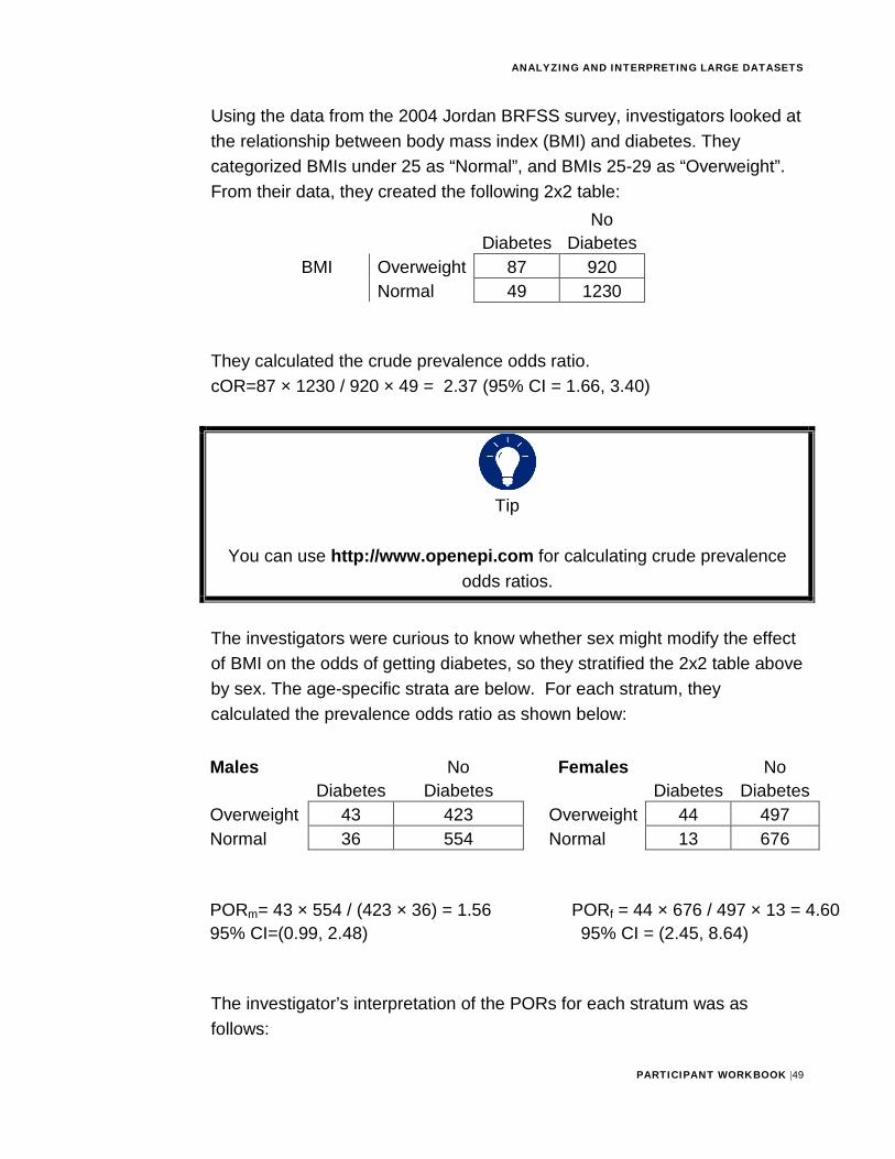
Using the data from the 2004 Jordan BRFSS survey, investigators looked at the relationship between body mass index (BMI) and diabetes. They categorized BMIs under 25 as “Normal”, and BMIs 25-29 as “Overweight”. From their data, they created the following 2x2 table:
Diabetes No
Diabetes BMI Overweight 87 920
Normal 49 1230
They calculated the crude prevalence odds ratio. cOR=87 × 1230 / 920 × 49 = 2.37 (95% CI = 1.66, 3.40)
Tip
You can use http://www.openepi.com for calculating crude prevalence odds ratios.
The investigators were curious to know whether sex might modify the effect of BMI on the odds of getting diabetes, so they stratified the 2x2 table above by sex. The age-specific strata are below. For each stratum, they calculated the prevalence odds ratio as shown below:
Males Diabetes
No Diabetes
Females Diabetes
No Diabetes
Overweight 43 423 Overweight 44 497 Normal 36 554 Normal 13 676
PORm= 43 × 554 / (423 × 36) = 1.56 PORf = 44 × 676 / 497 × 13 = 4.60 95% CI=(0.99, 2.48) 95% CI = (2.45, 8.64)
The investigator’s interpretation of the PORs for each stratum was as follows:
ANALYZING AND INTERPRETING LARGE DATASETS
PARTICIPANT WORKBOOK |50
The odds of having diabetes among males who are overweight is 1.6 times higher than among males with normal BMI. In contrast, the odds of having diabetes among overweight women was 4.6 times higher than among women with normal BMI.
Are the stratum-specific PORs different from each other?
In the example shown above, 4.6 is a much higher ratio measure of effect than 1.6; therefore, it would seem that the PORs are different. However, there are two more rigorous ways to evaluate whether or not there is a difference between the PORs:
1. Use a statistical test to determine whether or not the strata are differentfrom each other. For this test, the null hypothesis is that the strata areequal (H0: PORm=PORf). In OpenEpi and Epi Info, the programs willshow the results of the Breslow-Day test for Heterogeneity, a statisticaltest that determines whether the strata are different. A p-value of <0.05is usually considered to indicate that the strata are different.
Using OpenEpi, the p-value of the Breslow-Day test for Heterogeneity (or “Interaction”) is 0.006678. Since the p-value is <0.05, we would conclude that the strata are indeed different. This difference suggests that there may be a biological difference between men and women which augments the effect of being overweight on the risk of developing diabetes among women.
2. A less formal way of assessing EMM is to look at the confidenceintervals around each stratum-specific measure. If the confidenceintervals overlap, you could conclude that the stratum-specific measuresare not different from each other. There is no EMM present.
In the example shown above, the confidence intervals around the POR for males is from 0.99 to 2.48. The confidence intervals around the POR for females is from 2.45 to 8.64. Do they overlap? The upper CI for males (2.48) is slightly greater than the lower CI for females (2.45).

ANALYZING AND INTERPRETING LARGE DATASETS
PARTICIPANT WORKBOOK |51
Because they overlap slightly, it may be a matter of personal judgment as to whether the strata are different.
ANALYZING AND INTERPRETING LARGE DATASETS
PARTICIPANT WORKBOOK |52
CONFOUNDINGConfounding is a “mixing” of effects that occurs when a third factor distorts the true association between the exposure and disease. This is a type of bias. We need to control for it in our analysis, if it exists. Like other types of bias, confounding results in a mistaken estimate of an exposure’s effect on the risk of the outcome (e.g. disease). However, unlike most types of bias, we can sometimes control for it in our analysis.
To be a confounder, three criteria must be met. 1. A variable must be a risk factor for the outcome2. A variable must be associated with the exposure3. A variable must not be in the causal pathway between the exposure and
outcome
As an example, look at the effect of alcohol (the exposure) on developing lung cancer (the outcome). This relationship could be confounded by smoking. Let’s see if smoking fits the three requirements to be a confounder: 1. Smoking is a risk factor for lung cancer even in the absence of alcohol2. Smoking is associated with alcohol use (i.e. drinkers are more likely to
smoke than the general population)
3. Smoking is not caused by use of alcohol (i.e., smoking is not in the causal pathway between use of alcohol and lung cancer)
Thus, smoking meets the criteria for being a possible confounder.
Controlling for Confounding Removing the distortion caused by a confounding factor is called “controlling.” Controlling for confounding will result in a better, more valid measure of effect.
As discussed previously, stratification—as with modeling–allows you to compare like with like. By stratifying on sex, for example, you will compare the effect of an exposure exclusively among men and exclusively among women. If the effects are similar in the two groups, then techniques are
ANALYZING AND INTERPRETING LARGE DATASETS
PARTICIPANT WORKBOOK |53
available to calculate a summary or adjusted or “pooled” effect measure that eliminates confounding.
Assessing for Confounding The steps to assess for confounding are as follows: 1. Compute the stratum-specific measures of association2. Calculate the measures of effect stratified by levels of the potential
confounder3. Compare the stratum-specific measures to each other.
a. If the stratum-specific measures are different from each other, asdescribed in the EMM section, the covariate is an effect measuremodifier. Report the stratum-specific measures of association.
b. If the stratum-specific measures are not substantially differentfrom each other, compare the crude measure to the stratifiedmeasures.
i. If the crude measure and the stratified measures are closein value, the covariate has no impact on the exposure-outcome relationship. Report the crude measure.
c. If the stratified measures are close in value, but the crude isdifferent, then the covariate is a confounder. Take steps tocontrol confounding by using one of two approaches:
i. Calculate the adjusted measure of association that controlsfor confounding. If the crude measure differs from theadjusted measure by more than 10%, then confounding ispresent. Use the adjusted measure.
ii. Look at the range of stratum-specific measures. If thecrude measure is outside the range of the stratum-specificmeasures, then confounding is present. Calculate and usethe adjusted measure.
ANALYZING AND INTERPRETING LARGE DATASETS
PARTICIPANT WORKBOOK |54
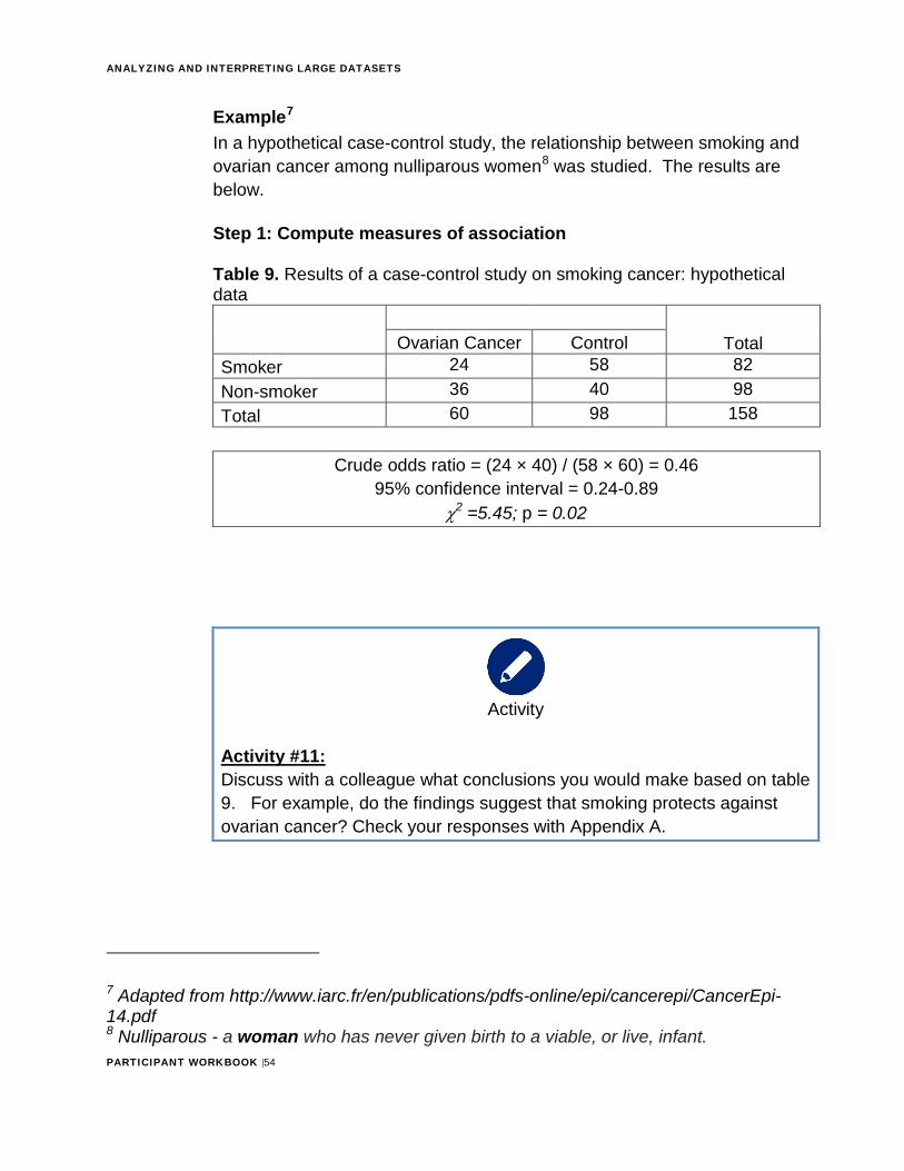
Example7 In a hypothetical case-control study, the relationship between smoking and ovarian cancer among nulliparous women8 was studied. The results are below.
Step 1: Compute measures of association
Table 9. Results of a case-control study on smoking cancer: hypothetical data
Ovarian Cancer Control Total Smoker 24 58 82 Non-smoker 36 40 98 Total 60 98 158
Crude odds ratio = (24 × 40) / (58 × 60) = 0.46 95% confidence interval = 0.24-0.89
χ2 =5.45; p = 0.02
Activity
Activity #11: Discuss with a colleague what conclusions you would make based on table 9. For example, do the findings suggest that smoking protects againstovarian cancer? Check your responses with Appendix A.
7 Adapted from http://www.iarc.fr/en/publications/pdfs-online/epi/cancerepi/CancerEpi-14.pdf8 Nulliparous - a woman who has never given birth to a viable, or live, infant.
ANALYZING AND INTERPRETING LARGE DATASETS
PARTICIPANT WORKBOOK |55
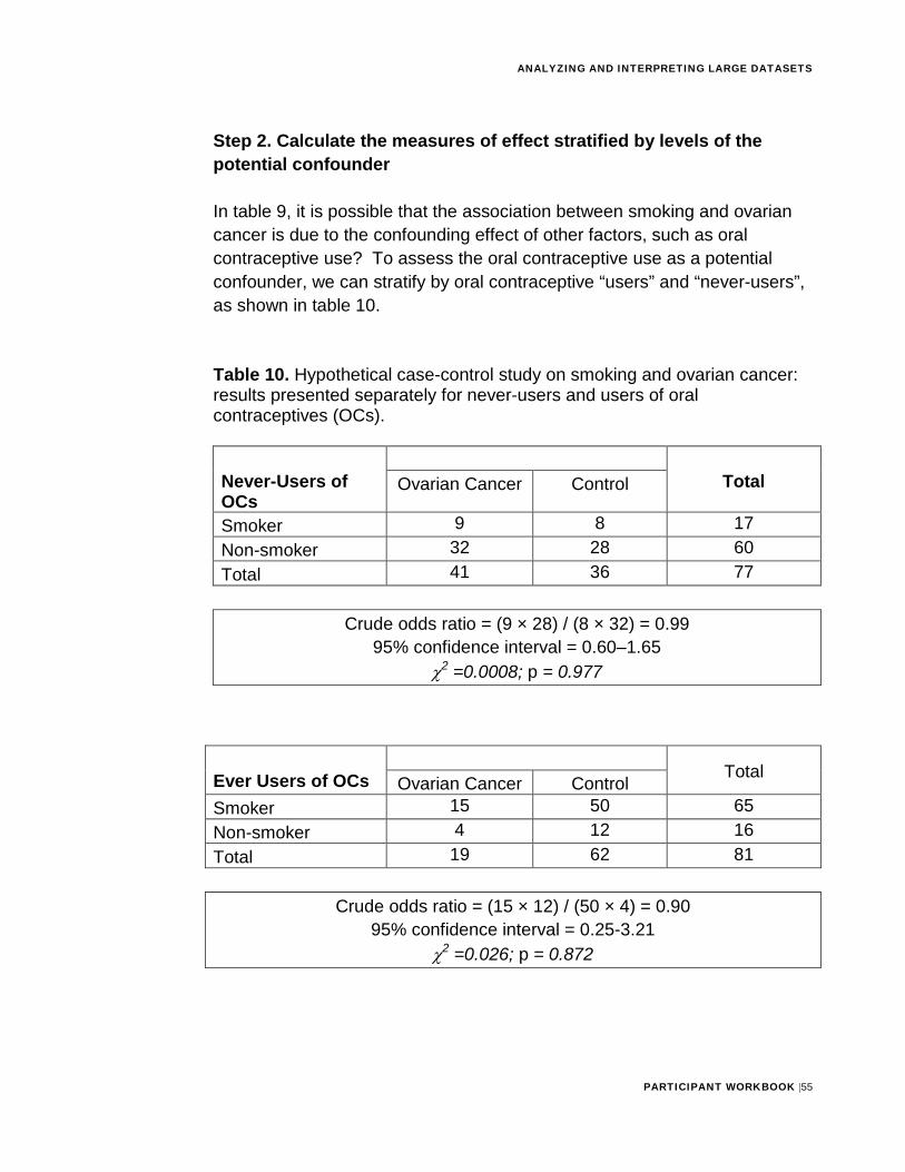
Step 2. Calculate the measures of effect stratified by levels of the potential confounder
In table 9, it is possible that the association between smoking and ovarian cancer is due to the confounding effect of other factors, such as oral contraceptive use? To assess the oral contraceptive use as a potential confounder, we can stratify by oral contraceptive “users” and “never-users”, as shown in table 10.
Table 10. Hypothetical case-control study on smoking and ovarian cancer: results presented separately for never-users and users of oral contraceptives (OCs).
Never-Users of OCs
Ovarian Cancer Control Total
Smoker 9 8 17 Non-smoker 32 28 60 Total 41 36 77
Crude odds ratio = (9 × 28) / (8 × 32) = 0.99 95% confidence interval = 0.60–1.65
χ2 =0.0008; p = 0.977
Total Ever Users of OCs Ovarian Cancer Control Smoker 15 50 65 Non-smoker 4 12 16 Total 19 62 81
Crude odds ratio = (15 × 12) / (50 × 4) = 0.90 95% confidence interval = 0.25-3.21
χ2 =0.026; p = 0.872
ANALYZING AND INTERPRETING LARGE DATASETS
PARTICIPANT WORKBOOK |56
Step 3. Compare the crude measure to the stratified measures
Activity
Activity #12: Discuss with a colleague the following question: Given an odds ratio of 0.90 in non-OC users and 0.99 in OC users, what value would be a reasonable summary of the two stratum specific effects? Check your responses with Appendix A.
The crude odds ratio was 0.46. The stratum-specific odds ratios were 0.99 and 0.90. Obviously, 0.46 is not within the range of 0.90 to 0.99, and hence the crude is not a reasonable summary of the relationship between smoking and ovarian cancer. The adjusted (Mantel-Haenszel) odds ratio is 0.95, with a 95% confidence interval of 0.42–2.16). Thus, the adjusted odds ratio is just what we expected. The confidence interval includes 1.0, indicating that we cannot exclude the null hypothesis; we cannot reject the assertion that smoking is not associated with ovarian cancer at all.
ANALYZING AND INTERPRETING LARGE DATASETS
PARTICIPANT WORKBOOK |57
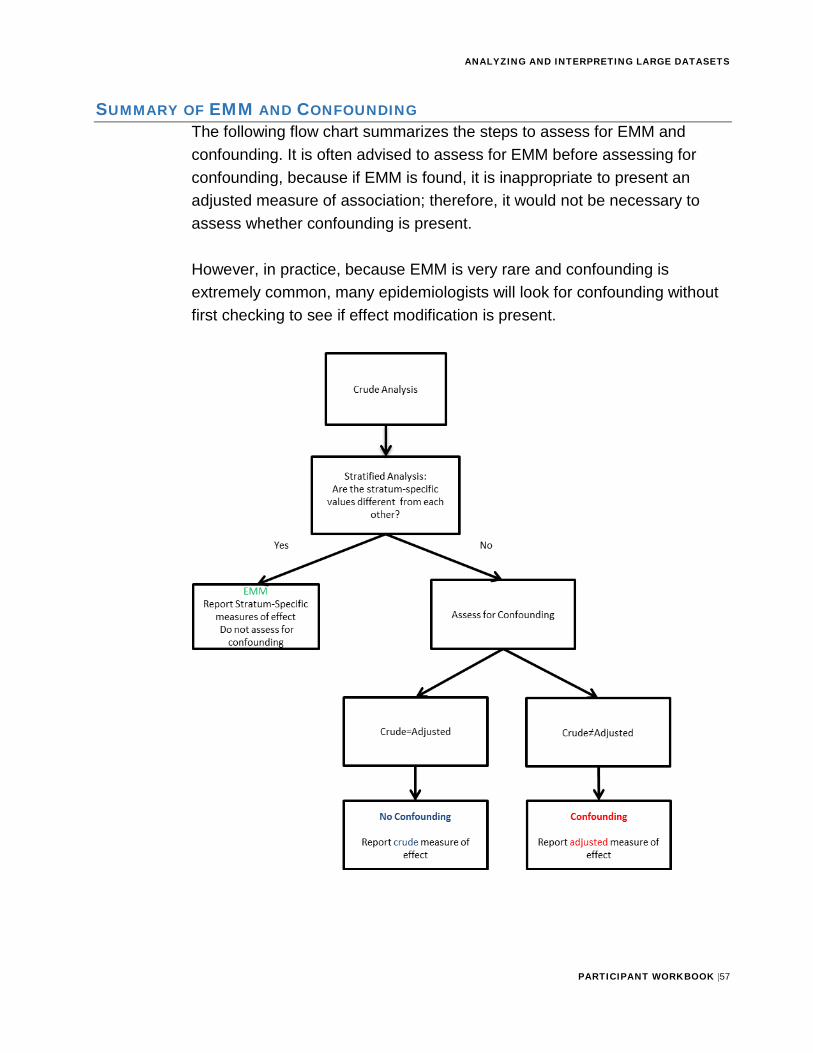
SUMMARY OF EMM AND CONFOUNDINGThe following flow chart summarizes the steps to assess for EMM and confounding. It is often advised to assess for EMM before assessing for confounding, because if EMM is found, it is inappropriate to present an adjusted measure of association; therefore, it would not be necessary to assess whether confounding is present.
However, in practice, because EMM is very rare and confounding is extremely common, many epidemiologists will look for confounding without first checking to see if effect modification is present.
ANALYZING AND INTERPRETING LARGE DATASETS
PARTICIPANT WORKBOOK |58
Stop
Let the facilitator or mentor know you are ready for a group discussion. He or she will review key concepts of assessing for potential confounders and
EMM before you complete Exercise 4.
KEY POINTS TO REMEMBERUse the space below to record any key points from the facilitator-led discussion:
ANALYZING AND INTERPRETING LARGE DATASETS
PARTICIPANT WORKBOOK |59
Activity
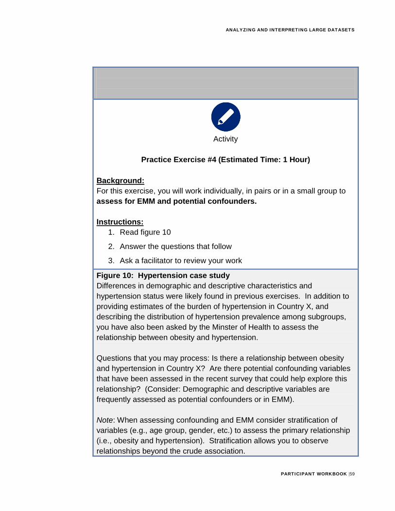
Practice Exercise #4 (Estimated Time: 1 Hour)
Background: For this exercise, you will work individually, in pairs or in a small group to assess for EMM and potential confounders.
Instructions: 1. Read figure 10
2. Answer the questions that follow
3. Ask a facilitator to review your work
Figure 10: Hypertension case study Differences in demographic and descriptive characteristics and hypertension status were likely found in previous exercises. In addition to providing estimates of the burden of hypertension in Country X, and describing the distribution of hypertension prevalence among subgroups, you have also been asked by the Minster of Health to assess the relationship between obesity and hypertension.
Questions that you may process: Is there a relationship between obesity and hypertension in Country X? Are there potential confounding variables that have been assessed in the recent survey that could help explore this relationship? (Consider: Demographic and descriptive variables are frequently assessed as potential confounders or in EMM).
Note: When assessing confounding and EMM consider stratification of variables (e.g., age group, gender, etc.) to assess the primary relationship (i.e., obesity and hypertension). Stratification allows you to observe relationships beyond the crude association.
ANALYZING AND INTERPRETING LARGE DATASETS
PARTICIPANT WORKBOOK |60
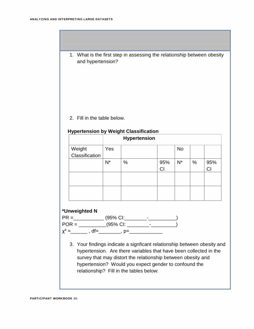
1. What is the first step in assessing the relationship between obesityand hypertension?
2. Fill in the table below.
Hypertension by Weight Classification Hypertension
Weight Classification
Yes No
N* % 95% CI
N* % 95% CI
*Unweighted NPR =___________ (95% CI:________-__________) POR = __________(95% CI: ________-_________) χ² =______ , df=________, p=____________
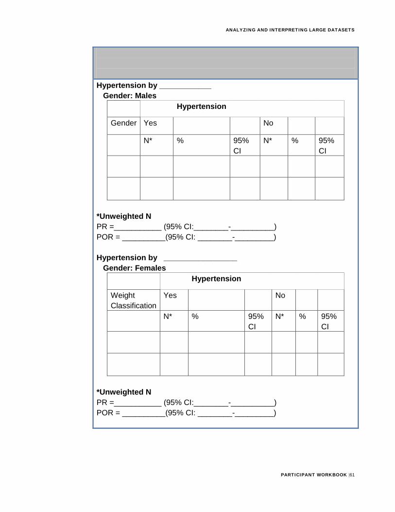
3. Your findings indicate a signficant relationship between obesity andhypertension. Are there variables that have been collected in thesurvey that may distort the relationship between obesity andhypertension? Would you expect gender to confound therelationship? Fill in the tables below:
ANALYZING AND INTERPRETING LARGE DATASETS
PARTICIPANT WORKBOOK |61
Hypertension by ____________ Gender: Males
Hypertension
Gender Yes No
N* % 95% CI
N* % 95% CI
*Unweighted NPR =___________ (95% CI:________-__________) POR = __________(95% CI: ________-_________)
Hypertension by _________________ Gender: Females
Hypertension
Weight Classification
Yes No
N* % 95% CI
N* % 95% CI
*Unweighted NPR =___________ (95% CI:________-__________) POR = __________(95% CI: ________-_________)
ANALYZING AND INTERPRETING LARGE DATASETS
PARTICIPANT WORKBOOK |62
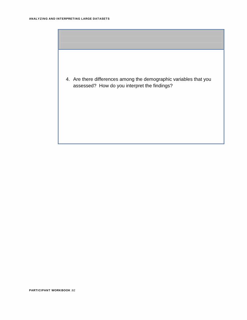
4. Are there differences among the demographic variables that youassessed? How do you interpret the findings?
ANALYZING AND INTERPRETING LARGE DATASETS
PARTICIPANT WORKBOOK |63
Section 4: Interpreting and Reporting Your Findings
The final step in data analysis is interpreting and reporting your results. Interpretation means translating your raw findings (measures of association, results of statistical tests) into words that explain what each result means and how it helps to answer your research question. Throughout this module, you have been asked to interpret your findings.
Let us practice interpreting the results of the case-control study to evaluate whether or not alcohol is a risk factor for coronary heart disease. Recall that in this study, the researchers compared people who drank more than three alcoholic drinks a day to people who drank three or fewer drinks a day. The results yielded an OR of 1.61, with a 95% confidence interval of (1.03, 2.54) and a χ2 value of 4.75, with a corresponding p-value of 0.029.
Activity
Activity #13: Discuss with a colleague the following question: How would you interpret these findings? Use the space below to record your response. Check your response with Appendix A.
ANALYZING AND INTERPRETING LARGE DATASETS
PARTICIPANT WORKBOOK |64
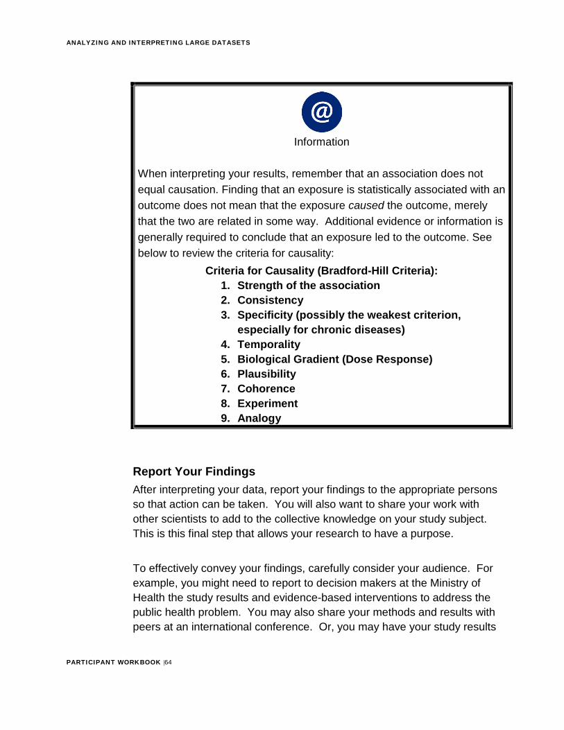
Information
When interpreting your results, remember that an association does not equal causation. Finding that an exposure is statistically associated with an outcome does not mean that the exposure caused the outcome, merely that the two are related in some way. Additional evidence or information is generally required to conclude that an exposure led to the outcome. See below to review the criteria for causality:
Criteria for Causality (Bradford-Hill Criteria): 1. Strength of the association2. Consistency3. Specificity (possibly the weakest criterion,
especially for chronic diseases)4. Temporality5. Biological Gradient (Dose Response)6. Plausibility7. Cohorence8. Experiment9. Analogy
Report Your Findings After interpreting your data, report your findings to the appropriate persons so that action can be taken. You will also want to share your work with other scientists to add to the collective knowledge on your study subject. This is this final step that allows your research to have a purpose.
To effectively convey your findings, carefully consider your audience. For example, you might need to report to decision makers at the Ministry of Health the study results and evidence-based interventions to address the public health problem. You may also share your methods and results with peers at an international conference. Or, you may have your study results
ANALYZING AND INTERPRETING LARGE DATASETS
PARTICIPANT WORKBOOK |65
published in a scientific journal. If you have received funding from a donor to conduct your study, they will surely be interested in your findings, too!
The way in which you report your findings will depend on your audience. If the audience is other epidemiologists, you can generally communicate your findings using technical terminology. However, many ministers and ministry of health staff are not epidemiologists or statisticians; they may not know what an odds ratio or risk ratio is or how to interpret one. They will still be knowledgeable about public health matters and will want to know how your findings can help to protect the population’s health. Translate your findings into language that they will understand.
Similarly, there will be times when it is necessary to share your findings with non-scientific audiences such as the media, law enforcement, and the community. These groups will need to know and understand the results of your study in order to make certain decisions. Use simple messages and non-technical language.
Regardless of who the audience is, simply telling people what you found is not enough; you must also provide them actionable recommendations for what to do.
Consider how you might report the results to your minister of health and other public health decision makers with regards to the CHD and alcohol study.
Activity
Activity #14: Write a short synopsis of the findings, along with a recommendation, in the space below. Check your responses with Appendix A.
ANALYZING AND INTERPRETING LARGE DATASETS
PARTICIPANT WORKBOOK |66
Activity
Activity #15 Write a short summary of your findings and recommendations that will be disseminated to the public via the media Check your responses with Appendix A.
ANALYZING AND INTERPRETING LARGE DATASETS
PARTICIPANT WORKBOOK |67
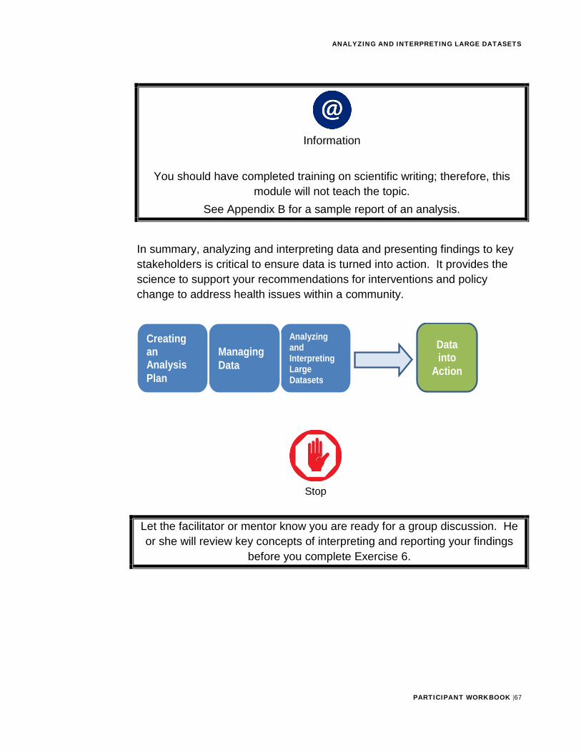
Information
You should have completed training on scientific writing; therefore, this module will not teach the topic.
See Appendix B for a sample report of an analysis.
In summary, analyzing and interpreting data and presenting findings to key stakeholders is critical to ensure data is turned into action. It provides the science to support your recommendations for interventions and policy change to address health issues within a community.
Stop
Let the facilitator or mentor know you are ready for a group discussion. He or she will review key concepts of interpreting and reporting your findings
before you complete Exercise 6.
Data into
Action
Analyzing and Interpreting Large Datasets
Managing Data
Creating an Analysis Plan
ANALYZING AND INTERPRETING LARGE DATASETS
PARTICIPANT WORKBOOK |68
Activity
Practice Exercise #5 (Estimated Time: 45 Minutes)
Background: For this exercise, you will work individually to summarize your findings and prepare a report based on the hypertension analysis.
Instructions: 1. Read Figure 11
2. Answer the questions below
3. Ask a facilitator to review your work
Figure 11. As you recall, the Minister has asked you to report the findings of the national health survey data. The Minister wants to provide the report to the national and provincial decision-makers to better understand the magnitude of the burden of disease and the key determinants and underlying factors that are affecting this public health burden. The Minister is hoping use your findings to target resources and support evidence-based actions and policies to improve the health of the population.
Questions:
1. Based on the results of your analyses, use the space below to
ANALYZING AND INTERPRETING LARGE DATASETS
PARTICIPANT WORKBOOK |69
summarize your key key findings.
2. What main sections would you include in the report? List in thespace below.
3. Which of the tables you created would you include in the report tosupport your findings? Describe them in the space below.
4. Would you recommend changes to the national survey to better
ANALYZING AND INTERPRETING LARGE DATASETS
PARTICIPANT WORKBOOK |70
assess hypertension in Country X?
Stop
Activity
Complete the Skill Assessment.
ANALYZING AND INTERPRETING LARGE DATASETS
PARTICIPANT WORKBOOK |71
Resources
For more information on component/item nonresponse adjustment and re-weighting the data for analyses:
Lohr, Sharon L. Sampling: Design and Analysis, pp.265-272. Duxbury Press, 1999; and
Examples of papers with re-weighted NHANES data
Gregg E, Sorlie P, Paulose-Ram R, Gu Q, Wolz M, Eberhardt MS, Burt VL, Engelgau MM, and Geiss LS. Prevalence of lower extremity disease among persons 40 years and older in the US with and without diabetes. Diabetes Care. 2004 Jul;27(7):1591-7.
Ostchega Y, Dillon CF, Lindle R, Carroll M, Hurley BF. Isokinetic leg muscle strength in older americans and its relationship to a standardized walk test: data from the national health and nutrition examination survey 1999-2000. J Am Geriatr Soc. 2004 Jun;52(6):977-82.
Other references:
Dicker, RC. Analyzing and interpreting data. In: GreggMB, editor. Field Epidemiology. 2nd ed. 2002, New York: Oxford University Press;. P. 132-172.
Elliott, A. Statistical Analysis Quick Reference Guidebook: With SPSS Examples.1st Ed. California: Sage; 2006.
Kleinbaum DG, Kupper LL, Morgenstern H. Epidemiologic research: Principles and quanitative methods. New York: Van Nostrand Reinhold; 1982.
Rothman, K. Greenland, S. Lash, T. Modern Epidemiology. 3rd Ed. Pennsylvania: Lippincott Williams & Wilkins; 2008
Jekel, J. Katz, D. Wild, D. Elmore, J. Epidemiology, Biostatistics and Preventive Medicine. 3rd Ed. Pennsylvania: Saunders; 2007.

ANALYZING AND INTERPRETING LARGE DATASETS
PARTICIPANT WORKBOOK |72
Appendices
ANALYZING AND INTERPRETING LARGE DATASETS
PARTICIPANT WORKBOOK |73
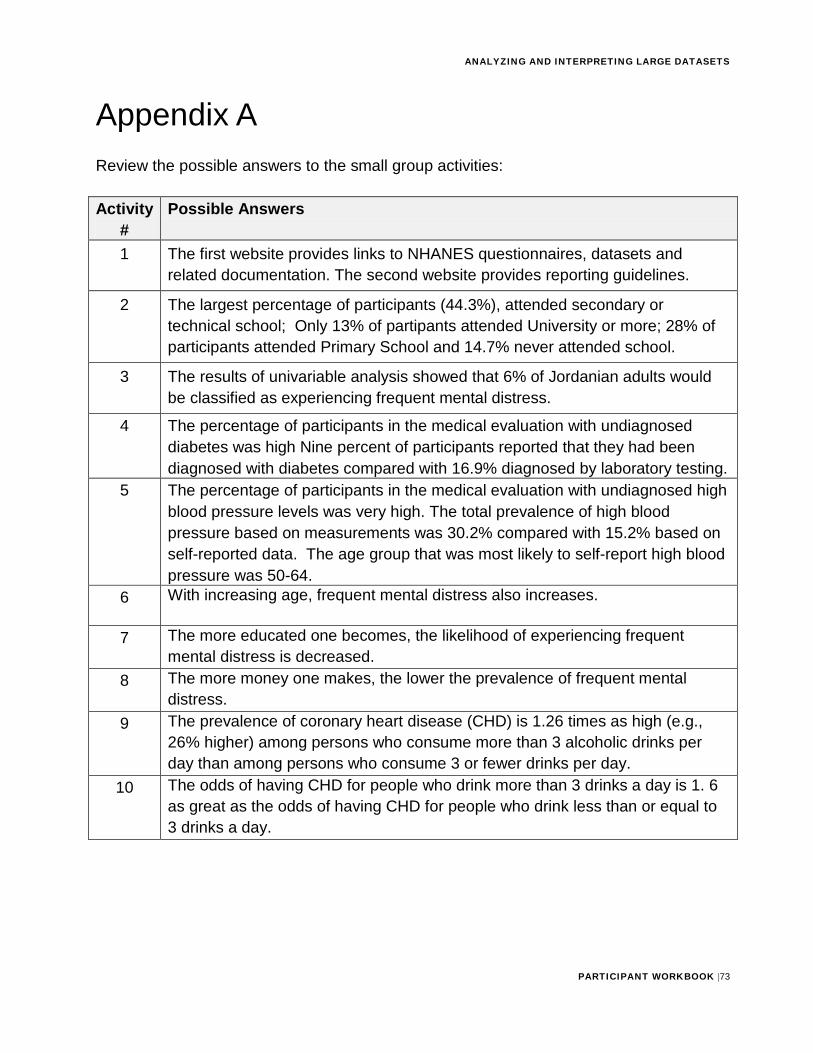
Appendix A Review the possible answers to the small group activities:
Activity #
Possible Answers
1 The first website provides links to NHANES questionnaires, datasets and related documentation. The second website provides reporting guidelines.
2 The largest percentage of participants (44.3%), attended secondary or technical school; Only 13% of partipants attended University or more; 28% of participants attended Primary School and 14.7% never attended school.
3 The results of univariable analysis showed that 6% of Jordanian adults would be classified as experiencing frequent mental distress.
4 The percentage of participants in the medical evaluation with undiagnosed diabetes was high Nine percent of participants reported that they had been diagnosed with diabetes compared with 16.9% diagnosed by laboratory testing.
5 The percentage of participants in the medical evaluation with undiagnosed high blood pressure levels was very high. The total prevalence of high blood pressure based on measurements was 30.2% compared with 15.2% based on self-reported data. The age group that was most likely to self-report high blood pressure was 50-64.
6 With increasing age, frequent mental distress also increases.
7 The more educated one becomes, the likelihood of experiencing frequent mental distress is decreased.
8 The more money one makes, the lower the prevalence of frequent mental distress.
9 The prevalence of coronary heart disease (CHD) is 1.26 times as high (e.g., 26% higher) among persons who consume more than 3 alcoholic drinks per day than among persons who consume 3 or fewer drinks per day.
10 The odds of having CHD for people who drink more than 3 drinks a day is 1. 6 as great as the odds of having CHD for people who drink less than or equal to 3 drinks a day.
ANALYZING AND INTERPRETING LARGE DATASETS
PARTICIPANT WORKBOOK |74
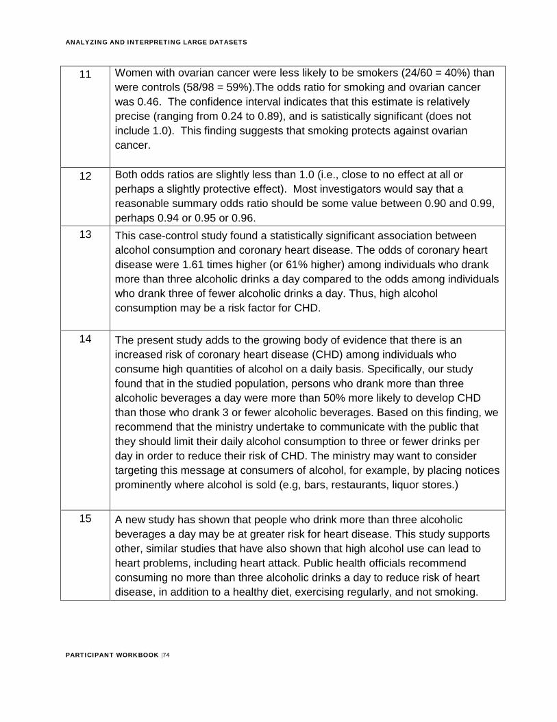
11 Women with ovarian cancer were less likely to be smokers (24/60 = 40%) than were controls (58/98 = 59%).The odds ratio for smoking and ovarian cancer was 0.46. The confidence interval indicates that this estimate is relatively precise (ranging from 0.24 to 0.89), and is satistically significant (does not include 1.0). This finding suggests that smoking protects against ovarian cancer.
12 Both odds ratios are slightly less than 1.0 (i.e., close to no effect at all or perhaps a slightly protective effect). Most investigators would say that a reasonable summary odds ratio should be some value between 0.90 and 0.99, perhaps 0.94 or 0.95 or 0.96.
13 This case-control study found a statistically significant association between alcohol consumption and coronary heart disease. The odds of coronary heart disease were 1.61 times higher (or 61% higher) among individuals who drank more than three alcoholic drinks a day compared to the odds among individuals who drank three of fewer alcoholic drinks a day. Thus, high alcohol consumption may be a risk factor for CHD.
14 The present study adds to the growing body of evidence that there is an increased risk of coronary heart disease (CHD) among individuals who consume high quantities of alcohol on a daily basis. Specifically, our study found that in the studied population, persons who drank more than three alcoholic beverages a day were more than 50% more likely to develop CHD than those who drank 3 or fewer alcoholic beverages. Based on this finding, we recommend that the ministry undertake to communicate with the public that they should limit their daily alcohol consumption to three or fewer drinks per day in order to reduce their risk of CHD. The ministry may want to consider targeting this message at consumers of alcohol, for example, by placing notices prominently where alcohol is sold (e.g, bars, restaurants, liquor stores.)
15 A new study has shown that people who drink more than three alcoholic beverages a day may be at greater risk for heart disease. This study supports other, similar studies that have also shown that high alcohol use can lead to heart problems, including heart attack. Public health officials recommend consuming no more than three alcoholic drinks a day to reduce risk of heart disease, in addition to a healthy diet, exercising regularly, and not smoking.

ANALYZING AND INTERPRETING LARGE DATASETS
PARTICIPANT WORKBOOK |75
Appendix B
ANALYZING AND INTERPRETING LARGE DATASETS
PARTICIPANT WORKBOOK |76
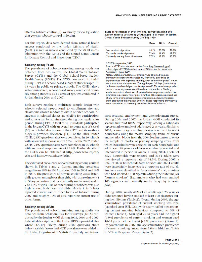
ANALYZING AND INTERPRETING LARGE DATASETS
PARTICIPANT WORKBOOK |77
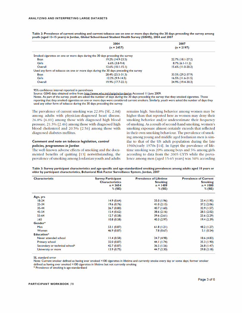
ANALYZING AND INTERPRETING LARGE DATASETS
PARTICIPANT WORKBOOK |78
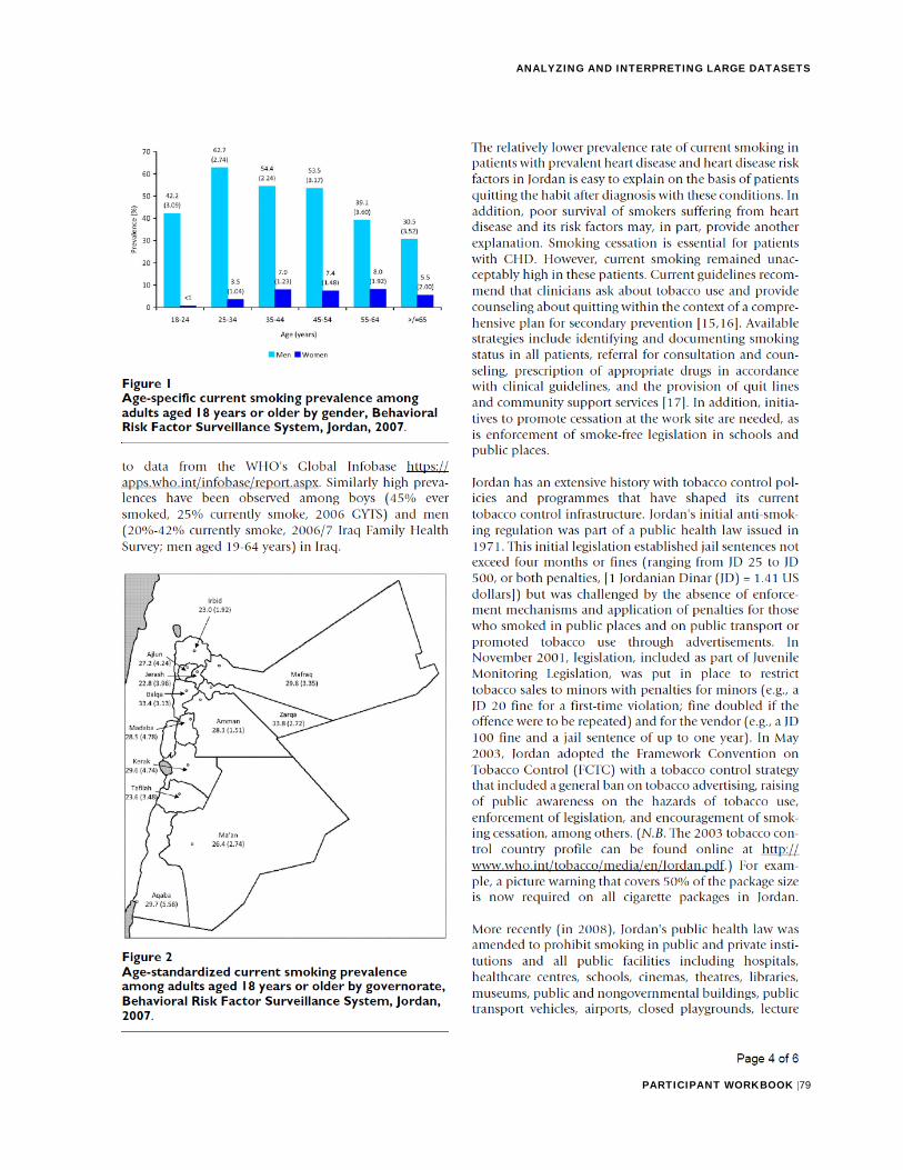
ANALYZING AND INTERPRETING LARGE DATASETS
PARTICIPANT WORKBOOK |79
ANALYZING AND INTERPRETING LARGE DATASETS
PARTICIPANT WORKBOOK |80