Analytical and Numerical Solutions of Boundary ValueProblems for the Regularized 13 Moment Equations

Henning Struchtrup, Peyman Taheri, and Anirudh Rana

Dept. of Mechanical Engineering, University of Victoria, PO Box 3055 STN CSC, Victoria BC V8W 3P6,Canada, e-mail: struchtr@uvic.ca

Abstract. Classical hydrodynamics—the laws of Navier-Stokes and Fourier—fails in the description of processes in rarefiedgases. For not too large Knudsen numbers, extended macroscopic models offer an alternative to the solution of the Boltzmannequations. Anlytical and numerical solutions show that the regularized 13 moment equations can capture all important linearand non-linear rarefaction effects with good accuracy.

Keywords: Rarefied gas flows, Microflows, Slip flow, Regularized 13-moment equationsPACS: 51.10.+y, 47.10.ab, 47.45.Gx, 05.70.Ln

INTRODUCTION

The accurate simulation of gas flows in microdevices requires effective transport models that allow for fast and accuratesolutions of gas microflows. Classical gas flows have small Knudsen numbers (ratio between average mean free pathand length scale of the flow), and can be described by the equations of classical hydrodynamics, i.e., the laws of Navier-Stokes and Fourier (NSF). For gas microflows, however, the Knudsen number is not sufficiently small to guarantee thevalidity of the NSF equations, and the processes must be modelled with more detailed theories.

The NSF equations solve for the macroscopic quantities mass density ρ (xk, t), velocity vi (xk, t) and temperatureT (xk, t), at all locations xk and all times t. The Boltzmann equation [1, 2], which gives the detailed microscopicdescription of gas flows at all Knudsen numbers, is an equation for the particle velocity distribution f (xk, t,ck), theinteresting macroscopic quantities, e.g., ρ ,vi,T , follow from suitable averaging over the particle velocity ck.

The NSF equations can be derived from the Boltzmann equation in the limit of sufficiently small Knudsen numbers[1, 2]. There are several methods to derive macroscopic equation systems that go beyond the capabilities of the NSFequations to describe rarefied gas flows. We shall show that, with some limitations, certain extended transport modelsare able to describe rarefied gas flows with Knudsen numbers Kn . 1 with sufficient accuracy.

Outside the hydrodynamic regime, that is for Kn & 0.01, many interesting phenomena—rarefaction effects, whichdo not arise in standard hydrodynamics—are found in experiments, and from the Boltzmann equation. The touchstonefor any extended transport model is its capability to describe as many of these as possible. Some significant rarefactionphenomena are: (a) heat flux in flow direction without temperature gradient [3]; (b) non-constant pressure profile inCouette and Poiseuille flows [4]; (c) in Poiseuille flow the mass flow exhibits a minimum for Knudsen numbers aroundunity [5–7] and (d) there is a characteristic dip in the temperature profile [4]; (e) transpiration flow, that is flow inducedby a temperature gradient in the wall [7]; (f) Knudsen boundary layers at the walls [2]; (g) phase speed and attenuationof high frequency sound waves differ from the prediction of classical hydrodynamics [8]; (h) the detailed structure ofshock waves cannot be reproduced by classical hydrodynamics [9].

The earliest derivation of the Navier-Stokes and Fourier laws from the Boltzmann equation used the Chapman-Enskog (CE) expansion to first order in the Knudsen number [1]. The application of the CE method to higher ordersgives the Burnett [10] and super-Burnett equations [1, 2], which are unstable in time dependent problems [11].Moreover, the Burnett equations lack a complete set of boundary conditions, and they are not appropriate for Knudsenlayers [2]. For a detailed review of the literature on Burnett-type equations see [12].

In Grad’s moment method the space of macroscopic variables is extended by including stress tensor σ i j, heat fluxvector qi, and other moments of the distribution function [13, 14]. The resulting equations are stable [2], and, if thenumber of variables is sufficiently large, can describe Knudsen layers [15]. The Grad method does not state how many,and which, variables are required for flows with a given Knudsen number. While Grad provided a theory of boundaryconditions for his equations [13], only few solutions of boundary value problems are available in the literature [16].

Since 2003 we are involved in the development and evaluation of the regularized 13 moment (R13) equationswhich are of third order in the Knudsen number, i.e., of super-Burnett order [9, 14, 17–19]. Their rational derivationfrom the Boltzmann equation [2, 18, 19] combines elements of the CE and Grad methods with new ideas, and theequations combine the benefits of Grad and Burnett-type equations, while omitting their problems. The R13 equationsare linearly stable [2, 18, 19]; give accurate predictions for phase speeds and damping of ultrasound waves [2, 18];give smooth shock structures for all Mach numbers [9]; exhibit Knudsen boundary layers [18]; are furnished with acomplete theory of boundary conditions [20, 21]; and obey an H-theorem for the linear case [22].

With this, the R13 equations currently represent the most successful extended hydrodynamic model at Burnett orsuper-Burnett order. They give reliable results for Knudsen numbers up to Kn . 0.5. While the model was developedfor 13 moments, all ideas (derivation, boundary conditions, numerical methods, . . . ) can be applied to larger momentnumbers. This extends the validity of the model to larger Knudsen numbers [2]: Gu and Emerson have developed andsolved the R26 moment equations which give reliable results up to Kn . 1.0 [23, 24].

A particularly important feature of the R13 and R26 equations is that they are accessible to analytical solutions ofboundary value problems, even for somewhat non-linear processes [22, 25–29]. Moreover, suitable numerical methodsallow their fast solution for steady state problems by avoiding time stepping into equilibrium [20].

In the remainder of the paper we give an overview over our ongoing work on the equations. We will focus onsolutions for particular problems, and comparison to benchmark solutions obtained from kinetic theory. For theoreticalbackground and additional references the reader is referred to the cited literature.

R13 EQUATIONS

While we shall also present solutions of the R13 equations in cylindrical geometry, in order to save space, we showthem only in standard rectangular coordinates, and we shall only consider the equations for Maxwell molecules[2, 18, 19]. The R13 equations consist of the conservation laws for mass, momentum and energy, ( D

Dt = ∂∂ t + vk

∂∂ xk

–

convective derivative, θ = km T – temperature in energy units, p = ρθ – pressure)

DρDt

+∂ρvk

∂xk= 0 , ρ

Dvi

Dt+

∂ p∂xi

+∂σ ik

∂xk= 0 ,

32

ρDθDt

+∂qk

∂xk=−(pδ i j +σ i j)

∂vi

∂x j. (1)

These are extended by full moment equations for stress and heat flux (indices in angular brackets indicate trace-freesymmetric tensors, σ kk = 0),

Dσ i j

Dt+σ i j

∂vk

∂xk+

45

∂q〈i∂x j〉

+2σ k〈i∂v j〉∂xk

+∂mi jk

∂xk+2p

∂v〈i∂x j〉

=− pµ

σ i j , (2)

Dqi

Dt+

52

σ ik∂θ∂xk

+θ∂σ ik

∂xk−θσ ik

∂ lnρ∂xk

+75

qk∂vi

∂xk+

25

qk∂vk

∂xi

+75

qi∂vk

∂xk+

12

∂Rik

∂xk+

16

∂∆∂xi

+mi jk∂v j

∂xk− σ i j

ρ∂σ jk

∂xk+

52

p∂θ∂xi

=−23

pµ

qi . (3)

For small Kundsen numbers, these two equations reduce to the laws of Navier-Stokes and Fourier (underlined terms).For larger Knudsen numbers, the complete equations must be considered, together with constitutive equations for thehigher moments ∆, Ri j, mi jk. In Grad’s classical 13 moment equations these vanish [13, 14], ∆|G = Ri j|G = mi jk|G = 0.

For the R13 equations, the constitutive equations are obtained from higher order moment equations by carefulconsideration of the order of magnitude of all moments, and their influence in the conservation laws [2, 9, 18, 19],

∆ =−σ i jσ i j

ρ−12

µp

[θ

∂qk

∂xk+θσ kl

∂vk

∂xl+

72

qk∂θ∂xk

−qkθp

∂ p∂xk

],

Ri j =−47

1ρ

σ k〈iσ j〉k−245

µp

[θ

∂q〈i∂x j〉

+2q〈i∂θ∂x j〉

+107

θσ k〈i∂v〈 j〉∂xk〉

− θp

q〈i∂ p

∂x j〉

], (4)

mi jk =−2µp

[θ

∂σ 〈i j

∂xk〉+σ 〈i j

∂θ∂xk〉

+45

q〈i∂v j

∂xk〉−σ 〈i j

θp

∂ p∂xk〉

].

The appropriate phase density for the R13 equations is Grad’s phase density for 26 moments, where the highermoments are replaced by the constitutive relations (4). The terms added to the original Grad 13 moment equationsare of super-Burnett order, the CE expansion of the R13 equations reproduces the super-Burnett equations [2, 18]. Forsufficiently small Mach numbers (Ma≤Kn) the underlined terms in (4) contribute above the super-Burnett order, andmust be removed.

BOUNDARY CONDITIONS

A detailed discussion of the derivation of boundary conditions for the R13 equations, including the question how manyboundary conditions are required, is presented in [20]. The boundary conditions follow from the Maxwell boundarycondition [2] for the Boltzmann equation and the phase density for the R13 equations as [20, 21]

σ12 =− χ2−χ

√2

πθ

[P

(v1− vW

1)+

15

q1 +12

m122

]n2 ,

q2 =− χ2−χ

√2

πθ

[2P(θ −θW )− 1

2PV 2 +

12

θσ 22 +115

∆+5

28R22

]n2 ,

m112 =− χ2−χ

√2

πθ

[1

14R11 +θσ11− 1

5θσ22 +

15

P(θ −θW )− 45

PV 2 +1

150∆]

n2 , (5)

m222 =χ

2−χ

√2

πθ

[25

P(θ −θW )− 35

PV 2− 75

θσ22 +175

∆− 114

R22

]n2 ,

R12 =χ

2−χ

√2

πθ

[Pθ

(v1− vW

1)− 11

5q1− 1

2θm122−PV 3 +6PV (θ −θW )

]n2 .

Here, χ is the accommodation coefficient, vW1 and θW are the velocity and temperature of the wall, n2 is the wall

normal, and P = ρθ + 12 σ22 − 1

120∆θ − 1

28R22θ . Vanishing normal velocity, v2 = 0, is already incorporated. These

equations are appropriate for flow in plane channels, see [26, 29] for the expressions in cylindrical geometry.The first two equations describe velocity slip and temperature jump at the wall, the other equations are jump

equations for higher moments. For extended moment systems, e.g., the R26 equations, additional boundary conditionsare obtained from the same set of arguments [23, 24]. Second order slip conditions for the Navier-Stokes-Fourierequations can be obtained from the above by appropriate consideration of the Knudsen number order of the variouscontributions [26, 27, 29].

BULK EFFECTS AND KNUDSEN LAYERS

The early publications on the R13 equations focused on boundary free problems, in particular (a) their linear stability[18]; (b) their agreement with measured phase speeds and attenuation of ultrasound waves [18, 19]; (c) their ability topredict smooth shock structures [9]. The evaluation of the linearized equations showed that, other than the Burnett-typeequations, the R13 equations exhibit Knudsen boundary layers [2, 18].

The path to fitting-free solutions of boundary value problems was opened when Gu and Emerson applied Grad’sideas on boundary conditions to the R13 equations [21]. After the number of boundary conditions required for solutionwas clarified in [20], the door was open to solve the R13 equations for Couette and Poiseuille flow in flat andcylindrical geometries, for linear and non-linear transpiration flow, and some linear time dependent problems [25–29]. Corresponding results for the R26 equations in flat geometry are presented in [23, 24].

The R13 and R26 equations can be solved analytically, even for somewhat non-linear processes. As an example, westudy force driven Poiseuille flow between infinite resting parallel plates of uniform temperature θW [25]. This flowis dominated by shear, and thus quadratic terms in shear related quantities such as shear stress and velocity gradientswere kept in the R13 equations, while they were linearized else. The solutions for velocity, stress and temperature read

v1 = C1− G1x22

2Kn+

35

G1Kn− 25C3 cosh

√5x2

3Kn, σ12 = G1x2 , (6)

/H2x

¾12 q1

/H2x /H2x

v1

¾22 q2

/H2x /H2x /H2x

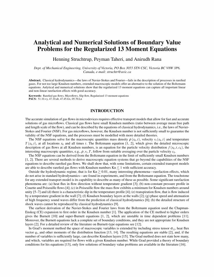
FIGURE 1. Force-driven Poiseuille flow with dimensionless force G1 = 0.2355. Profiles are computed for Kn = 0.072 (solidline), 0.15 (dashed line), 0.4 (dotted line), and 1.0 (dash-dot line); circles are DSMC simulations for Kn = 0.072 [25].

θ = θW +C2− 145

G21x4

2

Kn2 +488525

G21x2

2 +C3

[956375

G1Kncosh

√5x2

3Kn+

32σ12

35√

5sinh

√5x2

3Kn

]−C4

25

cosh

√5x2√6Kn

. (7)

Here, all quantities are made dimensionless, G1 is the force that drives the flow, and Cα are the integrating constantsthat are determined from the boundary conditions (5). Terms that would be present in the classical description of theprocess via the NSF equations are underlined.

The—un-underlined—rarefaction terms can be split into two groups: Knudsen layers, and bulk effects. All con-tributions with hyperbolic sine and cosine functions describe Knudsen layers, i.e., exponential decay away from thewall over few mean free paths. For small Knudsen numbers, the Knudsen layers are limited to the vicinity of the wall,but for larger Knudsen numbers they contribute to the flow anywhere in the domain. The other contributions are bulkeffects, most of which are non-linear in the driving force G1. For small Knudsen numbers these terms can be ignoredagainst the—underlined—hydrodynamic contributions, but for finite Knudsen numbers they contribute considerably.

In the equation for temperature θ the two terms G21

45Kn2

[−x42 + 1464

35 Kn2x22]

compete, which leads to a significant dipin the temperature curve. This dip can be found from analytical considerations of the Boltzmann equation and fromits numerical solution [4]. The second term is a super-Burnett term, thus this phenomenon can only be captured by amacroscopic model that is accurate to super-Burnett order.

Figure 1, reprinted from [25] where the complete solutions can be found, shows plots for the relevant moments fora variety of Knudsen numbers. The comparison to DSMC simulations shows good agreement. We point out that thetemperature θ and heat flux q2 are governed by non-linear bulk effects, while the heat flux q1 is governed by Knudsenlayers only, and the normal stress σ22 curve results from the interplay of Knudsen layers and bulk effects. Thus, thefigure gives good evidence that the R13 equations can describe both classes of rarefaction phenomena: Knudsen layersand (non-linear) bulk effects. Although there is no temperature gradient, there is a heat flux q1 in flow direction, themechanocaloric heat flux, which is well established in kinetic theory.

FLOW THROUGH CYLINDRICAL PIPES

Next, we present analytical solutions for the linearized and dimensionless equations that describe flow throughcylindrical pipes under pressure or temperature gradients [29]. We focus on axial velocity, shear stress, and the heat

NSFR13Siewert & Valougeorgis

Â=1.0

vz qz

r R/ r R/

Velocity profile in Poiseuille flowcomparison with BE data

(a)

Heat flux profile in Poiseuille flowcomparison with BE data

(b)

Kn=0.07

Kn=0.14

Kn=0.35

Â=1.0

NSF

R13

Siewert & Valougeorgis

NSF

1

2

Loyalka & Hamoodi

NSFR13Siewert & Valougeorgis

Â=1.0

Kn=0.35

Kn=0.14

Kn=0.07 vz qz

r R/ r R/

Velocity profile in transpiration flowcomparison with BE data

(c)

Heat flux profile in transpiration flowcomparison with BE data

(d)

Â=1.0

NSFR13Siewert &Valougeorgis

Kn=0.07

Kn=0.14

Kn=0.35

Kn=0.35

Kn=0.14

Kn=0.07

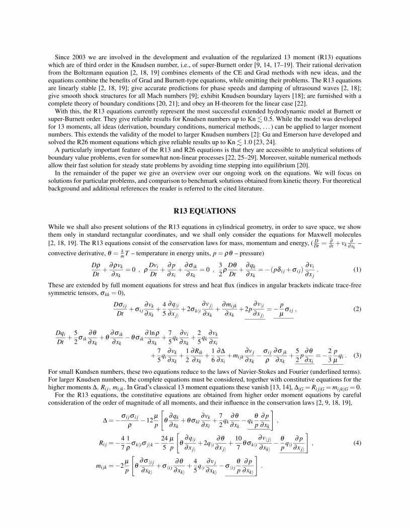
FIGURE 2. Radial distribution of velocity and heat flux in Poiseuille flow (a,b) and transpiration flow (c,d) for χ = 1 andKn = {0.07,0.14,0.35}. For Poiseuille flow, NSF with first-order slip condition (NSF1), NSF with second-order slip condition(NSF2), and R13 equations with third-order boundary conditions (R13) are compared to the Boltzmann equation (BE) [30, 31]. Fortranspiration flow, NSF and R13 are compared to the Boltzmann equation (BE) [30, 31].

flux parallel to the flow.For Poiseuille flow under a dimensionless pressure gradient ℘ one finds [29]

vz = C1 +℘

4Knr2− 2

5qz , σ rz =−℘

2r , qz = C2 J0

(√59

rKn

)+

32

Kn℘. (8a)

For thermal creep flow under a dimensionless temperature gradient τ one finds [29]

vz = C1− 25

qz , σ rz = 0 , qz = C2 J0

(√59

rKn

)− 15Kn

4τ . (9a)

Here, r is the dimensionless pipe radius, and C1, C2 are the integrating constants, which follow from the boundaryconditions. As before, the underlined terms indicate the solution for the NSF equations. Due to the geometry, Knudsenlayers are given by the zeroth-order Bessel function J0. In Poiseuille flow the term 3

2 Kn℘describes a higher-order bulkeffect (heat flux without temperature gradient), while in transpiration flow we recognize the Fourier heat conductionforced by the axial temperature gradient τ . Figure 2 shows the radial distribution of velocity and heat flux for χ = 1and Kn = {0.07,0.14,0.35}.

Poiseuille flow: Plot (a) compares the velocity solution for R13 and NSF with linear Boltzmann equation (BE)data. For the small Knudsen number Kn = 0.07, all models show good agreement with the kinetic solution. As theKnudsen number increases, NSF with first-order slip condition yield unsatisfactory bulk solution. By predicting alarger slip, the second-order slip condition shifts the NSF solution towards the R13 and kinetic results. Compared toNSF with second-order slip condition, R13 shows better agreement with kinetic data near the wall. In Plot (b), themechanocaloric heat flux qz is compared to BE data. This heat flow, which points in opposite direction to mass flow,cannot be predicted by NSF.

Transpiration flow: Plot (c) compares the velocity solution with linear Boltzmann equation (BE) data. NSF yieldsa plug flow across the tube cross section, and drastically overestimates the mass and heat fluxes near the wall. In plot(d), the axial heat flux is compared to BE data. This heat flow is a superposition of Fourier heat flow, i.e., the NSFsolution, and the mechanocaloric heat flow. R13, on the other hand, shows good agreement with DSMC.

When the pipe connects two reservoirs at different temperatures, the so-called thermomolecular pressure differencewill establish between the reservoirs. In steady state, temperature and pressure gradients point into the same direction,but induce flows in opposite directions. R13 predicts the velocity

vz = C1 +℘

4Knr2− 2

5

[C2 J0

(√59

rKn

)+

32

Kn℘− 154

Knτ

]. (10)

r R/

vz

Kn=0.10

Kn=0.15

Kn=0.20

r R/

}=0.3

}=0.5

(a) (b)

}=0.1 Kn=0.1

Kn

°

Â=0.6

Â=0.8

Â=1.0

¿=2.05

¿=1.19

¿=0.86

¿=10.25

¿=2.05

¿=6.15

}=0.1

(c)

vz

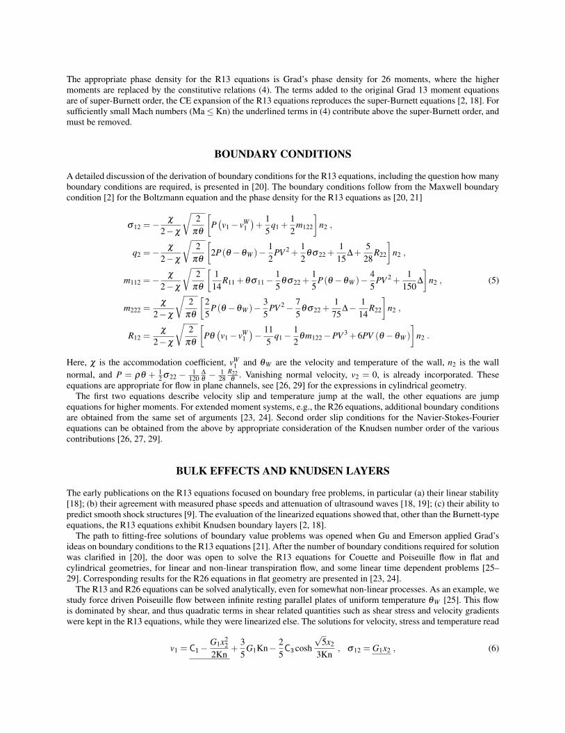
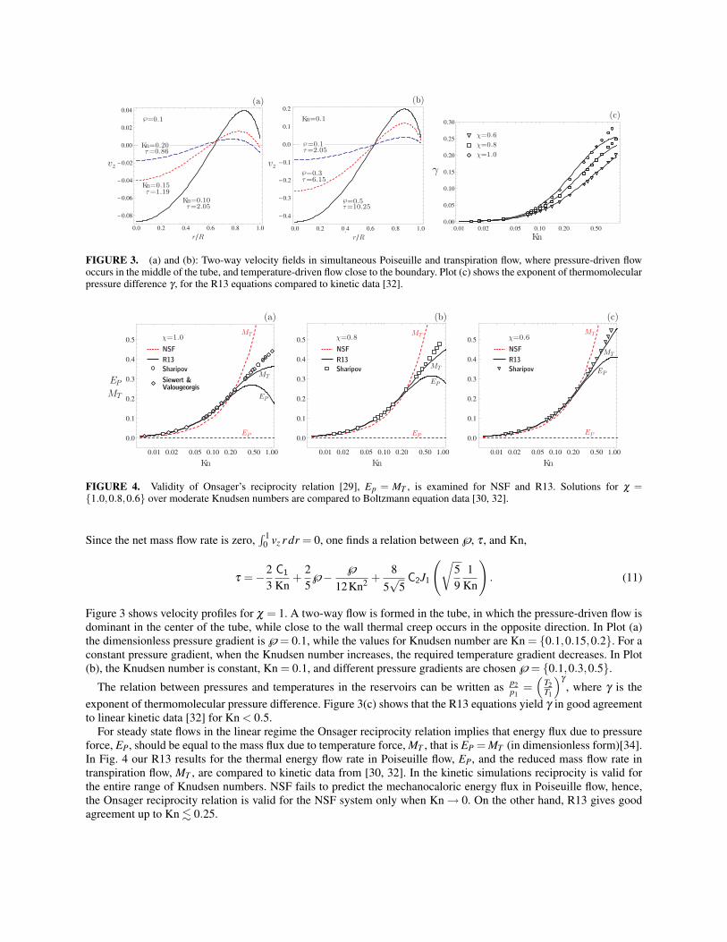
FIGURE 3. (a) and (b): Two-way velocity fields in simultaneous Poiseuille and transpiration flow, where pressure-driven flowoccurs in the middle of the tube, and temperature-driven flow close to the boundary. Plot (c) shows the exponent of thermomolecularpressure difference γ , for the R13 equations compared to kinetic data [32].

Kn Kn Kn

EP

MT

Â=1.0

R13

NSF

Siewert &Valougeorgis

Sharipov

MT

EP

MT

EP

MT

EP

MT

EP

MT

EP

MT

EP

(a) (b) (c)

Â=0.8

R13

NSF

Sharipov

Â=0.6

R13

NSF

Sharipov

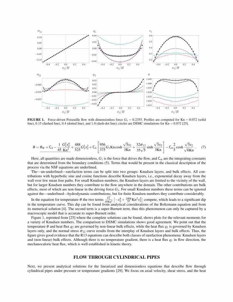
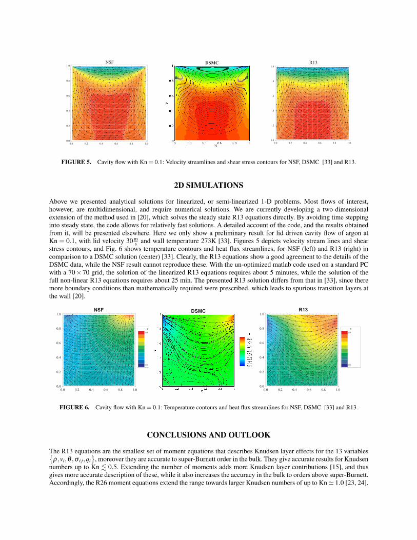
FIGURE 4. Validity of Onsager’s reciprocity relation [29], Ep = MT , is examined for NSF and R13. Solutions for χ ={1.0,0.8,0.6} over moderate Knudsen numbers are compared to Boltzmann equation data [30, 32].

Since the net mass flow rate is zero,∫ 1

0 vz r dr = 0, one finds a relation between ℘, τ , and Kn,

τ =−23

C1

Kn+

25

℘− ℘12Kn2 +

85√

5C2J1

(√59

1Kn

). (11)

Figure 3 shows velocity profiles for χ = 1. A two-way flow is formed in the tube, in which the pressure-driven flow isdominant in the center of the tube, while close to the wall thermal creep occurs in the opposite direction. In Plot (a)the dimensionless pressure gradient is ℘= 0.1, while the values for Knudsen number are Kn = {0.1,0.15,0.2}. For aconstant pressure gradient, when the Knudsen number increases, the required temperature gradient decreases. In Plot(b), the Knudsen number is constant, Kn = 0.1, and different pressure gradients are chosen ℘= {0.1,0.3,0.5}.

The relation between pressures and temperatures in the reservoirs can be written as p2p1

=(

T2T1

)γ, where γ is the

exponent of thermomolecular pressure difference. Figure 3(c) shows that the R13 equations yield γ in good agreementto linear kinetic data [32] for Kn < 0.5.

For steady state flows in the linear regime the Onsager reciprocity relation implies that energy flux due to pressureforce, EP, should be equal to the mass flux due to temperature force, MT , that is EP = MT (in dimensionless form)[34].In Fig. 4 our R13 results for the thermal energy flow rate in Poiseuille flow, EP, and the reduced mass flow rate intranspiration flow, MT , are compared to kinetic data from [30, 32]. In the kinetic simulations reciprocity is valid forthe entire range of Knudsen numbers. NSF fails to predict the mechanocaloric energy flux in Poiseuille flow, hence,the Onsager reciprocity relation is valid for the NSF system only when Kn → 0. On the other hand, R13 gives goodagreement up to Kn . 0.25.

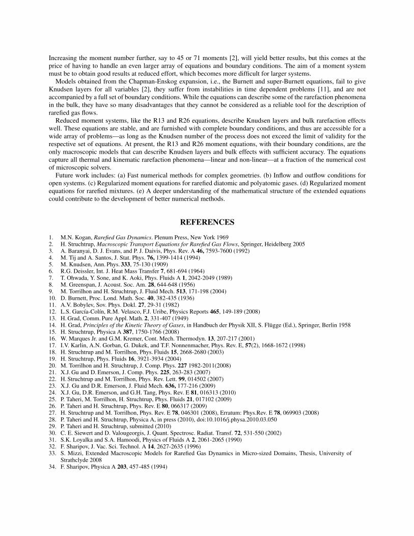
DSMC

FIGURE 5. Cavity flow with Kn = 0.1: Velocity streamlines and shear stress contours for NSF, DSMC [33] and R13.

2D SIMULATIONS

Above we presented analytical solutions for linearized, or semi-linearized 1-D problems. Most flows of interest,however, are multidimensional, and require numerical solutions. We are currently developing a two-dimensionalextension of the method used in [20], which solves the steady state R13 equations directly. By avoiding time steppinginto steady state, the code allows for relatively fast solutions. A detailed account of the code, and the results obtainedfrom it, will be presented elsewhere. Here we only show a preliminary result for lid driven cavity flow of argon atKn = 0.1, with lid velocity 30 m

s and wall temperature 273K [33]. Figures 5 depicts velocity stream lines and shearstress contours, and Fig. 6 shows temperature contours and heat flux streamlines, for NSF (left) and R13 (right) incomparison to a DSMC solution (center) [33]. Clearly, the R13 equations show a good agreement to the details of theDSMC data, while the NSF result cannot reproduce these. With the un-optimized matlab code used on a standard PCwith a 70× 70 grid, the solution of the linearized R13 equations requires about 5 minutes, while the solution of thefull non-linear R13 equations requires about 25 min. The presented R13 solution differs from that in [33], since theremore boundary conditions than mathematically required were prescribed, which leads to spurious transition layers atthe wall [20].

NSF R13DSMC

FIGURE 6. Cavity flow with Kn = 0.1: Temperature contours and heat flux streamlines for NSF, DSMC [33] and R13.

CONCLUSIONS AND OUTLOOK

The R13 equations are the smallest set of moment equations that describes Knudsen layer effects for the 13 variables{ρ,vi,θ ,σ i j,qi

}, moreover they are accurate to super-Burnett order in the bulk. They give accurate results for Knudsen

numbers up to Kn . 0.5. Extending the number of moments adds more Knudsen layer contributions [15], and thusgives more accurate description of these, while it also increases the accuracy in the bulk to orders above super-Burnett.Accordingly, the R26 moment equations extend the range towards larger Knudsen numbers of up to Kn' 1.0 [23, 24].

Increasing the moment number further, say to 45 or 71 moments [2], will yield better results, but this comes at theprice of having to handle an even larger array of equations and boundary conditions. The aim of a moment systemmust be to obtain good results at reduced effort, which becomes more difficult for larger systems.

Models obtained from the Chapman-Enskog expansion, i.e., the Burnett and super-Burnett equations, fail to giveKnudsen layers for all variables [2], they suffer from instabilities in time dependent problems [11], and are notaccompanied by a full set of boundary conditions. While the equations can describe some of the rarefaction phenomenain the bulk, they have so many disadvantages that they cannot be considered as a reliable tool for the description ofrarefied gas flows.

Reduced moment systems, like the R13 and R26 equations, describe Knudsen layers and bulk rarefaction effectswell. These equations are stable, and are furnished with complete boundary conditions, and thus are accessible for awide array of problems—as long as the Knudsen number of the process does not exceed the limit of validity for therespective set of equations. At present, the R13 and R26 moment equations, with their boundary conditions, are theonly macroscopic models that can describe Knudsen layers and bulk effects with sufficient accuracy. The equationscapture all thermal and kinematic rarefaction phenomena—linear and non-linear—at a fraction of the numerical costof microscopic solvers.

Future work includes: (a) Fast numerical methods for complex geometries. (b) Inflow and outflow conditions foropen systems. (c) Regularized moment equations for rarefied diatomic and polyatomic gases. (d) Regularized momentequations for rarefied mixtures. (e) A deeper understanding of the mathematical structure of the extended equationscould contribute to the development of better numerical methods.

REFERENCES

1. M.N. Kogan, Rarefied Gas Dynamics. Plenum Press, New York 19692. H. Struchtrup, Macroscopic Transport Equations for Rarefied Gas Flows, Springer, Heidelberg 20053. A. Baranyai, D. J. Evans, and P. J. Daivis, Phys. Rev. A 46, 7593-7600 (1992)4. M. Tij and A. Santos, J. Stat. Phys. 76, 1399-1414 (1994)5. M. Knudsen, Ann. Phys. 333, 75-130 (1909)6. R.G. Deissler, Int. J. Heat Mass Transfer 7, 681-694 (1964)7. T. Ohwada, Y. Sone, and K. Aoki, Phys. Fluids A 1, 2042-2049 (1989)8. M. Greenspan, J. Acoust. Soc. Am. 28, 644-648 (1956)9. M. Torrilhon and H. Struchtrup, J. Fluid Mech. 513, 171-198 (2004)10. D. Burnett, Proc. Lond. Math. Soc. 40, 382-435 (1936)11. A.V. Bobylev, Sov. Phys. Dokl. 27, 29-31 (1982)12. L.S. García-Colín, R.M. Velasco, F.J. Uribe, Physics Reports 465, 149-189 (2008)13. H. Grad, Comm. Pure Appl. Math. 2, 331-407 (1949)14. H. Grad, Principles of the Kinetic Theory of Gases, in Handbuch der Physik XII, S. Flügge (Ed.), Springer, Berlin 195815. H. Struchtrup, Physica A 387, 1750-1766 (2008)16. W. Marques Jr. and G.M. Kremer, Cont. Mech. Thermodyn. 13, 207-217 (2001)17. I.V. Karlin, A.N. Gorban, G. Dukek, and T.F. Nonnenmacher, Phys. Rev. E, 57(2), 1668-1672 (1998)18. H. Struchtrup and M. Torrilhon, Phys. Fluids 15, 2668-2680 (2003)19. H. Struchtrup, Phys. Fluids 16, 3921-3934 (2004)20. M. Torrilhon and H. Struchtrup, J. Comp. Phys. 227 1982-2011(2008)21. X.J. Gu and D. Emerson, J. Comp. Phys. 225, 263-283 (2007)22. H. Struchtrup and M. Torrilhon, Phys. Rev. Lett. 99, 014502 (2007)23. X.J. Gu and D.R. Emerson, J. Fluid Mech. 636, 177-216 (2009)24. X.J. Gu, D.R. Emerson, and G.H. Tang, Phys. Rev. E 81, 016313 (2010)25. P. Taheri, M. Torrilhon, H. Struchtrup, Phys. Fluids 21, 017102 (2009)26. P. Taheri and H. Struchtrup, Phys. Rev. E 80, 066317 (2009)27. H. Struchtrup and M. Torrilhon, Phys. Rev. E 78, 046301 (2008), Erratum: Phys.Rev. E 78, 069903 (2008)28. P. Taheri and H. Struchtrup, Physica A, in press (2010), doi:10.1016/j.physa.2010.03.05029. P. Taheri and H. Struchtrup, submitted (2010)30. C. E. Siewert and D. Valougeorgis, J. Quant. Spectrosc. Radiat. Transf. 72, 531-550 (2002)31. S.K. Loyalka and S.A. Hamoodi, Physics of Fluids A 2, 2061-2065 (1990)32. F. Sharipov, J. Vac. Sci. Technol. A 14, 2627-2635 (1996)33. S. Mizzi, Extended Macroscopic Models for Rarefied Gas Dynamics in Micro-sized Domains, Thesis, University of

Strathclyde 200834. F. Sharipov, Physica A 203, 457-485 (1994)