analysis of two-axis sun tracking system - core · analysis of two-axis sun tracking system by...
TRANSCRIPT

Analysis of Two-Axis Sun Tracking System
By
Elvan ARMAKAN
A Dissertation Submitted to the Graduate School in Partial Fulfillment of the
Requirements for the Degree of
MASTER OF SCIENCE
Department: Energy Engineering Major: Energy Engineering
(Energy and Power Systems)
Izmir Institute of Technology Izmir, Turkey
April, 2003

We approve the thesis of Elvan ARMAKAN
Date of Signature
03.04.2003
Asst.Prof.Dr. Bülent YARDIMOĞLU
Supervisor
Department of Mechanical Engineering
03.04.2003
Prof.Dr. Gürbüz ATAGÜNDÜZ
Head of Interdisciplinary
Energy Engineering (Energy and Power Systems)
03.04.2003
Asst.Prof.Dr. Serhan ÖZDEMİR
Department of Mechanical Engineering
03.04.2003
Prof.Dr. Gürbüz ATAGÜNDÜZ
Head of Interdisciplinary
Energy Engineering (Energy and Power Systems)

ACKNOWLEDGEMENTS
First of all, I particularly would like to thank my advisor, Asst.Prof.Dr. Bülent
YARDIMOĞLU, for his continuous guidance, support and vision that he never
hesitated to share, without which this study would not become a reality.
I also owe a great deal of thanks to Erdal BULĞAN, who I have worked
together with throughout the period of this exciting and wonderful study, for sharing his
experience with me and for his never ending technical and personal support.
I would like to take this opportunity to express my gratitude to Prof.Dr. Gürbüz
ATAGÜNDÜZ and Asst.Prof.Dr. Serhan ÖZDEMİR for agreeing to be in my thesis
defense committee.
I also would like to take this opportunity to thank Prof.Dr. Zeynel TUNCA and
Asst.Prof.Dr. Serhan ÖZDEMİR for their advices.
I sincerely thank my parents, and girlfriend for their support and encouragement.
I

ABSTRACT
In this study, a two-axis sun tracking system with an open loop computer control
is analyzed. For this purpose, a gyroscope-like prototype with two degrees of freedom is
designed. In order to control the prototype and track the sun all along the day, computer
software based on astronomical equations is developed. Beside the software, an
electronic circuit ensuring communication layer in between computer and the prototype
is designed and manufactured.
Software determining the sun position precisely and controlling the prototype is
developed utilizing a Visual Basic compiler on a Pentium IV 1600 MHz computer.
Input-output signals in between the computer and the electronic circuit is managed
through the parallel port (LPT) of the computer. Control of the prototype motors are
performed by amplifying the sun position-related computer signals on the electronic
circuitry.
Critical components of three-dimensional system model created in
Computer-Aided Design (CAD) and Computer-Aided Engineering (CAE) software are
analyzed from statical aspect. In addition, mathematical model of the system and its
stability analysis is generated in Matlab/Simulink software.
Last, a fixed-type photovoltaic cell and a two-axis sun tracking photovoltaic cell
satisfying a particular tracking sensitivity are theoretically analyzed and compared. A
two-axis sun tracking system working to fulfill a specific tracking sensitivity is
theoretically seen to provide about 40 % higher energy gain when compared to a fixed
system under extraterrestrial solar radiation.
II
ÖZ
Bu çalışmada, açık devre bilgisayar kontrollü iki eksenli güneş takip sistemi
incelenmiştir. Bu amaçla iki serbestlik derecesine sahip jiroskop benzeri bir prototip
dizayn edilmiştir. Prototipin kontrolü ve gün boyu güneş takibi için, astronomik
denklemlere dayalı bir bilgisayar yazılımı geliştirilmiştir. Bu yazılımın yanısıra
bilgisayar ile prototip arasında veri iletişimini sağlayan bir elektronik devre tasarlanarak
üretilmiştir.
Güneşin gün içerisindeki konumunu hassas olarak belirleyen ve prototipi kontrol
eden bilgisayar yazılımı, bir Pentium IV 1600 MHz bilgisayar üzerinde Visual Basic
derleyicisi kullanılarak geliştirilmiştir. Bilgisayar ile elektronik devre arasındaki
giriş-çıkış sinyalleri, bilgisayarın paralel portu (LPT) üzerinden gerçekleştirilmektedir.
Bilgisayarca güneşin hareketine bağlı olarak üretilen kumanda sinyalleri, elektronik
devre tarafından yükseltilerek prototip motorlarının kumandası sağlanmaktadır.
Bilgisayar Destekli Tasarım (CAD) ve Bilgisayar Destekli Mühendislik (CAE)
yazılımları kullanılarak oluşturulan üç boyutlu modelin tehlikeli parçaları statik açıdan
incelenmiştir. Bunun yanısıra Matlab/Simulink yazılımı kullanılarak sistemin
matematiksel modeli oluşturulmuş ve model üzerinden kararlılık (stabilite) analizi
yapılmıştır.
Son olarak, sabit bir güneş pili ile belirli bir açısal hassasiyeti sağlayacak
biçimde iki eksende hareket eden güneş pili enerji kazanımı yönünden teorik olarak
incelenmiş ve karşılaştırılmıştır. Belirli bir açısal hassasiyet altında çalışan iki eksenli
güneş takip sisteminin, sabit bir sisteme göre dünya dışı güneş radyasyonu etkisi
altında teorik hesaplamada yaklaşık % 40 daha fazla enerji kazancı sağladığı
görülmüştür.
III

TABLE OF CONTENTS
TABLE OF CONTENTS................................................................................................ IV
NOMENCLATURE ......................................................................................................VII
LIST OF FIGURES ......................................................................................................... X
LIST OF TABLES.........................................................................................................XII
Chapter 1........................................................................................................................... 1
INTRODUCTION ............................................................................................................ 1
Chapter 2........................................................................................................................... 4
SOLAR CALCULATION................................................................................................ 4
2.1 Introduction........................................................................................................ 4
2.2 Theoretical Basis................................................................................................ 5
2.2.1 Solar Radiation .................................................................................................. 5
2.2.2 The Relations between Sun and Earth Positions ............................................... 6
2.2.2.1 Introduction........................................................................................................ 6
2.2.2.2 Latitude φ and Longitude λ ................................................................................ 7
2.2.2.3 Time Zone.......................................................................................................... 7
2.2.2.4 Daylight Saving DS ........................................................................................... 7
2.3 Astronomic Considerations................................................................................ 8
2.3.1 Time Argument.................................................................................................. 8
2.3.2 Celestial Coordinate for the Sun........................................................................ 9
2.3.3 Solar Declination δ .......................................................................................... 11
2.3.4 Equation of Time EoT ..................................................................................... 12
2.3.5 Local Solar Time ............................................................................................. 13
2.3.6 Hour Angle ω................................................................................................... 14
2.3.7 Solar Altitude Angle αs.................................................................................... 14
2.3.8 Solar Azimuth Angle γs ................................................................................... 15
2.3.9 Sunrise and Sunset ........................................................................................... 15
2.3.10 Incidence Angle θ ............................................................................................ 16
2.4 Sun Position Calculation Software .................................................................. 16
IV

Chapter 3......................................................................................................................... 19
STRUCTURAL ANALYSIS ......................................................................................... 19
3.1 Introduction...................................................................................................... 19
3.2 Wind Load ....................................................................................................... 21
3.3 Static Analysis ................................................................................................. 21
3.3.1 Introduction...................................................................................................... 21
3.3.2 Panel 21
3.3.3 Shaft-1.............................................................................................................. 24
3.3.4 Shaft-2.............................................................................................................. 26
3.4 Stepper Motor Selection Process ..................................................................... 29
3.5 System Analysis............................................................................................... 30
3.5.1 Introduction...................................................................................................... 30
3.5.2 Mathematical Model of Stepper Motors.......................................................... 31
3.5.3 Disturbance Effect ........................................................................................... 37
3.5.4 Overall Mathematical Model ........................................................................... 39
Chapter 4......................................................................................................................... 41
ACTUATORS AND CONTROL SYSTEM .................................................................. 41
4.1 Introduction...................................................................................................... 41
4.2 Stepper Motor .................................................................................................. 42
4.2.1 Stepper Motor Basics....................................................................................... 42
4.2.1.1 Introduction...................................................................................................... 42
4.2.1.2 Direction and Speed......................................................................................... 43
4.2.1.3 Torque.............................................................................................................. 43
4.2.1.4 Resonance ........................................................................................................ 45
4.2.2 Stepper Motor Types ....................................................................................... 45
4.2.3 Stepper Motor Selection .................................................................................. 46
4.2.4 Stepper Motor Driving Modes......................................................................... 47
4.2.5 Stepper Motor Driving Mode Selection........................................................... 48
4.3 Sensors ............................................................................................................. 48
V
4.3.1 Reference Sensors............................................................................................ 48
4.3.2 Cloudiness Sensor............................................................................................ 49
4.4 Control Software.............................................................................................. 49
4.5 Parallel Port...................................................................................................... 52
4.6 Control Board .................................................................................................. 55
Chapter 5......................................................................................................................... 58
RESULTS AND DISCUSSION..................................................................................... 58
5.1 Beam Radiation Acting on a Surface............................................................... 58
5.2 Energy Production versus Consumption.......................................................... 60
5.3 Optimum Tracking Frequency for Maximum Energy Gain ............................ 60
Chapter 6......................................................................................................................... 63
CONCLUSIONS ............................................................................................................ 63
REFERENCES ............................................................................................................... 64
APPENDIX A................................................................................................................A-I
APPENDIX B................................................................................................................B-I
APPENDIX C................................................................................................................C-I
APPENDIX D................................................................................................................D-I
APPENDIX E ................................................................................................................E-I
APPENDIX F ................................................................................................................ F-I
VI

NOMENCLATURE
Chapter 2
DS Daylight saving time
EoT Equation of the time [degree]
g Mean anomaly [degree]
L Mean longitude of the Sun (in degree)
LSoT Local Solar Time
LST Local Standard Time
long.local The local longitude
long.standard The local standard time zone
N The number of days from J2000
Nm The day of year
Ny The number of day gone by since J2000 to beginning of each year
UT Universal Time
α Right ascension [degree]
αs Solar altitude angle [degree]
β Surface altitude angle [degree]
βs Ecliptic latitude [degree]
γ Surface azimuth angle [degree]
γs Solar azimuth angle [degree]
δ Solar declination [degree]
ε Obliquity of ecliptic [degree]
θ The solar incident angle [degree]
λ Ecliptic longitude [degree]
φ Latitude [degree]
ω Hour Angle [degree]
ωsunrise Sunrise times
ωsunset Sunset times
VII
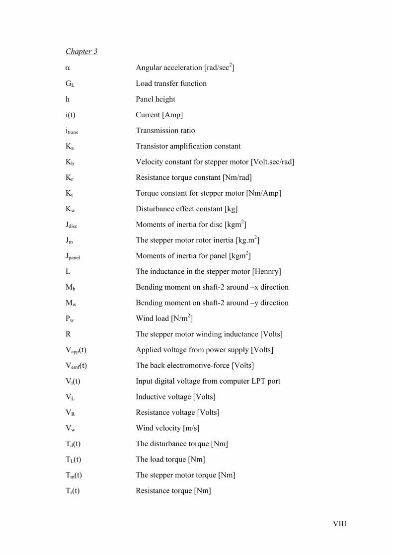
Chapter 3
α Angular acceleration [rad/sec2]
GL Load transfer function
h Panel height
i(t) Current [Amp]
itrans Transmission ratio
Ka Transistor amplification constant
Kb Velocity constant for stepper motor [Volt.sec/rad]
Kr Resistance torque constant [Nm/rad]
Kt Torque constant for stepper motor [Nm/Amp]
Kw Disturbance effect constant [kg]
Jdisc Moments of inertia for disc [kgm2]
Jm The stepper motor rotor inertia [kg.m2]
Jpanel Moments of inertia for panel [kgm2]
L The inductance in the stepper motor [Hennry]
Mb Bending moment on shaft-2 around –x direction
Mw Bending moment on shaft-2 around –y direction
Pw Wind load [N/m2]
R The stepper motor winding inductance [Volts]
Vapp(t) Applied voltage from power supply [Volts]
Vemf(t) The back electromotive-force [Volts]
Vi(t) Input digital voltage from computer LPT port
VL Inductive voltage [Volts]
VR Resistance voltage [Volts]
Vw Wind velocity [m/s]
Td(t) The disturbance torque [Nm]
TL(t) The load torque [Nm]
Tm(t) The stepper motor torque [Nm]
Tr(t) Resistance torque [Nm]
VIII

Ttm(t) Time constant [sec]
w Panel width [m]
βL The load viscous frictional efficient [Nm.sec]
βm The stepper motor viscous frictional coefficient [Nm.sec]
β The angle between panel and horizontal
ρ Air density [kg/m3]
θm Angular displacement for rotor [rad]
Chapter 5
A Photovoltaic cell area (m2)
Gb The beam radiation (W/m2)
Gbn The beam radiation on a plane normal (W/m2)
Gbt The beam radiation on a tilted plane (W/m2)
Gon The normal incident solar radiation (W/m2)
Gsc The solar constant (W/m2)
Ioperation Photovoltaic cell operating current (Amps)
Pconsumption Stepper motor energy consumption (Wh)
Pproduction Energy production on photovoltaic arrays (Wh)
Voperation Photovoltaic cell operating voltage (Volts)
IX

LIST OF FIGURES
Figure 2.1 The sun’s daily path across the sky [31] ......................................................... 4
Figure 2.2. Solar radiation types at ground level [17] ...................................................... 5
Figure 2.3 Earth’s orbit around the sun [28]..................................................................... 6
Figure 2.4 Latitude and longitude [29] ............................................................................. 7
Figure 2.5 Positional astronomy on the celestial sphere................................................ 10
Figure 2.6 The declination angle [28]............................................................................. 12
Figure 2.7 Variation of declination angle in a year ........................................................ 12
Figure 2.8 Equation of time in a year [6]........................................................................ 13
Figure 2.9 Solar altitude angle [28] ................................................................................ 15
Figure 2.10 Solar azimuth angle [28] ............................................................................. 15
Figure 2.11 Automatic calculation Graphical User Interface (GUI) .............................. 17
Figure 2.12 Manual calculation GUI .............................................................................. 18
Figure 3.1 The prototype of two axis sun tracking ......................................................... 20
Figure 3.2 Deflection analysis result of the panel in FEA.............................................. 22
Figure 3.3 Resultant deflection line and moment for panel............................................ 23
Figure 3.4 Resultant deflection line and moment for shaft-1 ......................................... 25
Figure 3.5 Moment acting on shaft-2.............................................................................. 27
Figure 3.6 Resultant deflection line and moment for shaft-2 ......................................... 28
Figure 3.7 A simple block diagram of the prototype’s stepper motor mechanism......... 30
Figure 3.8 A stepper motor schematic diagram.............................................................. 31
Figure 3.9 Stepper motor block diagram ........................................................................ 33
Figure 3.10 Single step response .................................................................................... 34
Figure 3.11 The damping ratio ξ and natural frequency ωn............................................ 35
Figure 3.12 Single step response for half step angle ...................................................... 36
Figure 3.13 The damping ratio ξ and natural frequency ωnf for half step angle ............. 36
Figure 3.14 Schematic panel illustration ........................................................................ 37
Figure 3.15 Disturbance effect component..................................................................... 38
X

Figure 3.16 Overall transfer function for two axis sun tracking system......................... 39
Figure 3.17 Sun tracking system overall transfer function............................................. 40
Figure 4.1 Flow diagram................................................................................................. 41
Figure 4.2 Stepper motor ................................................................................................ 42
Figure 4.3 Conceptual diagram of two-phases ............................................................... 43
Figure 4.4 The torque period versus position curve [33]................................................ 44
Figure 4.5 Stepper motor torque vs. angular displacement [33]..................................... 44
Figure 4.6 Hybrid stepper motor..................................................................................... 46
Figure 4.7 Cloudiness sensor’s circuit ............................................................................ 49
Figure 4.8 Automatic Control Graphical User Interface (GUI)...................................... 50
Figure 4.9 Manual Control GUI ..................................................................................... 51
Figure 4.10 Parallel Port logic levels.............................................................................. 52
Figure 4.11 The parallel port standard DB25 interface [36]........................................... 52
Figure 4.12 Electronic Circuit ........................................................................................ 56
Figure 4.13 Motorola 4N25 Optoisolator ....................................................................... 56
Figure 5.1 Beam radiation on horizontal and tilted surfaces. ......................................... 59
Figure 5.2 Energy Gain Comparison of fixed and two-axis sun tracking systems......... 61
Figure 5.3 Net Energy Gain............................................................................................ 62
XI

LIST OF TABLES
Table 2.1 Number of the days since the epoch J2000 to beginning of each year (Ny) ..... 8
Table 2.2 Days to beginning of month (Nm) [3]. i is calendar day. ................................. 9
Table 3.1 Technical characteristics of MDF and aluminum........................................... 19
Table 3.2 Maximum panel deflection ............................................................................. 22
Table 3.3 Maximum stress and maximum bending moment of panel............................ 24
Table 3.4 Maximum stress and maximum bending moment of shaft-1 ......................... 26
Table 3.5 Maximum stress and maximum bending moment of shaft-2 ......................... 28
Table 3.6 Stepper motor data list provided by Minebea Co.Ltd..................................... 34
Table 4.1 Half-step excitation sequence ......................................................................... 48
Table 4.2 Standard Parallel Port Addresses.................................................................... 53
Table 4.3 Data Lines....................................................................................................... 54
Table 4.4 Status Lines..................................................................................................... 54
Table 4.5 Control Lines .................................................................................................. 55
XII

Chapter 1
INTRODUCTION
The sun gives out an almost unlimited amount of energy, and on a clear sky,
there are about 1353 watts of free energy available for every square meter of land on
earth [6], [13]. The solar energy as a renewable resource seems to be suitable for
thermal and electricity forms of energy production.
The electricity can be produced from solar energy utilizing Photovoltaic Cell
(PV)’s. Although photovoltaic array of cells has such advantages as high reliability, low
construction and operating costs, and modularity [20], it has the disadvantage of being
inefficient for a single unit area. To overcome the existing disadvantage, either PV
material development or continuous movement of PV arrays to face the sun, called as
sun tracking, need to be accomplished. The underlying principle of the latter solution,
sun tracking, is to keep PV panels perpendicular to the sun rays as much technically and
economically as feasible.
As an example to the advantage of preferring sun tracking, a theoretical study
comparing useful energy gain for a fixed flat plate collector facing south with a one
allowed to track the sun is performed by Drago. The results of the work proved the fact that
the total useful energy gain of the fully tracking collector was 2.03 and 1.47 times
greater than that of the fixed single and double cover collector, respectively [19]. A
similar theoretical comparative study by Gandhidasan and Satcunanathan between fully
and semi-tracking flat plate collectors are performed. The outcomes of the research
demonstrated that semi-tracking collector rotating at 15 degrees per hour generated 20%
more energy than the stationary collector, and about 8% less energy than by the fully
tracking collector [21].
Satcunanathan [SATC83] performed an analytical and experimental study in
which the daily energy gain and hourly efficiencies of fixed collectors and
semi-tracking were compared. It was concluded that between 20 and 30% more energy
has been obtained with the semi tracking flat plate collector over the fixed one. Khalifa
et al [22] designed and constructed an electromechanical two-axis system and two
identical compound parabolic concentrators (CPC). Tests conducted on the two
identical fixed and tracking collectors draw the conclusion that a two-axis tracking
system may increase the thermal energy gain of a CPC collector by up to 75%.
1

Results of automatic sun tracking studies suggest the fact that having a small sun
tracking panel than having a static panel of a larger size may be more cost effective to
an extent even in the case of a single axis sun tracking. [20] In addition, deployment of
smaller panels has an advantage of lower heat losses, hence, higher efficiency.
Development in the technology, for example, the ones in the sun tracking panels,
maximizes energy gain and investment payback. With the help of digital computer
technology, the panels can continuously track the sun successfully. There are two types
of sun tracking methods; namely closed loop and open loop.
In closed loop sun tracking method, usually a set of luminosity sensors
continuously keep track of sun’s actual position for maximum solar radiation. For
instance, a microprocessor-based automatic sun tracking system proposed by Koyuncu
B. and Balasubramanian K. [23] harnessed closed loop control with measurement
feedbacks of two Light-Dependent Resistors (LDRs).
In open loop solar tracking, on the other hand, doesn't physically search for the
sun but instead, the sun position knowledge is obtained from a set of accurate
astronomical equations. For example, Mohamad M.A. et al [25] reported design and
implementation of one-axis system to track the mid-point of the sun trajectory every one
hour. Control structure in their study included an open loop microcomputer system
control through an interface circuit. The experiments proved that the electrical energy
collected by the tracked module increased about 25% of the tilted fixed one.
The purpose of this thesis is to track the sun all along the day to increase the PV
array efficiency. A gyroscope-like prototype as sun-tracking system having two-
degrees-of-freedom with open loop computer control is designed to track the sun. Open
loop control system is based on astronomical equations. A prototype is manufactured as
well.
In this study, the sun position is calculated at certain time intervals and the
control signals required are generated by the software based on astronomical equations.
The digital control signals are then transmitted to the control board through computer’s
parallel port. The digital signals are later on amplified to sufficient power levels by the
control board which is fed by external power supply of 12 Volts. Thus, the stepper
motors on the prototype is activated and rotated at certain angular displacements to
achieve calculated sun position angles.
2

This thesis is composed of five chapters. In order; Chapter 2 covers parameters
used in calculation of the sun position in the form of astronomical equations
meticulously. Besides, software to determine the sun position all day with respect to
local coordinates based on the aforementioned astronomical equations is explained
towards the end of Chapter 2.
Chapter 3 is concerned with the static, dynamic and stability analyses of the
prototype under such operating conditions as the wind. First, static analysis is
performed so as to check the strength of the prototype components under the worst-case
scenario. Next, the prototype is analyzed with the help of Computer-Aided Engineering
(CAE) tools under such dynamic loads as friction, inertia, etc. Last, system
characteristics are examined in the categories of system-order, settling time at a
particular tolerance band, and system sensitivity to both inertia and damping factor.
Chapter 4 consists of implementation details of the sun tracking approach
offered in this thesis study. Such components as actuators, sensors, control board and
parallel port specifications are expressed one by one.
Chapter 5 is concerned with the comparison between performance of a two-axis
sun tracking system and an identical fixed system. A two-axis sun tracking photovoltaic
cell satisfying a particular tracking sensitivity and a fixed-type photovoltaic cell are
analyzed and discussed.
Finally, in Chapter 6, conclusions are presented.
3

Chapter 2
SOLAR CALCULATION
2.1 Introduction
Due to the spin of the earth about its own axis and its orbiting around the sun,
position of the sun varies throughout the day and the season. The sun rises south of due
east in winter and north of due east in summer, and the sun’s path is higher in the sky in
summer than it is in winter [7]. The sun’s path across the sky at the solstices and
equinoxes are shown in Figure 2.1.
Figure 2.1 The sun’s daily path across the sky [31]
In two-axis sun tracking, exact sun position must be known. Thus, a software to
calculate accurate sun position all along the day via astronomical equations is developed
in the duration of this thesis. As input parameters to determine the sun’s path across the
sky, the location of the observer, time and date must be known.
4

2.2 Theoretical Basis
2.2.1 Solar Radiation
As the name implies, solar radiation is the radiation created by the sun. When the solar
radiation passes through the earth’s atmosphere, it is partially absorbed. Total or global
solar radiation received at ground level consists of direct and indirect radiation, shown
in Figure 2.2.
• Beam or direct radiation
• Diffuse or scattered radiation
• Albedo or reflected radiation
Figure 2.2. Solar radiation types at ground level [17]
Sunlight reaching the earth surface, which is unmodified by any of the above
atmospheric processes, is termed beam or direct radiation. It is the type of sunlight that
casts a sharp shadow, and on a sunny day it can be as much as 80 percent of the total
sunlight striking a surface [9]. Hence, beam or direct radiation is the most important
type of radiation for solar processes.
The second type of solar radiation is diffuse or scattered sunlight. This is such
sunlight that comes from all directions in the sky dome other than the direction of the
sun. It is the sunlight scattered by atmospheric components such as particles, water
vapor, and aerosols. On a cloudy day, the sunlight is 100 percent diffuse [9].
The third type of radiation is Albedo or reflected radiation. Incoming solar
radiation striking the earth surface is partially reflected and partially absorbed. Earth
surface reflectivity varies with covering material type. For solar collectors mounted on
5

the roof of a building, the amount of reflected radiation may relatively be small
compared to other radiation types [9].
The prototype’s panel is designed to absorb direct radiation. The sun motion is
important in determining the angle at which beam radiation strikes the panel surface.
2.2.2 The Relations between Sun and Earth Positions
2.2.2.1 Introduction
The earth revolves around the Sun in an elliptical orbit. It takes 365.2564 days
for the earth to travel around the sun and 23.9345 hours for the earth to complete a full
rotation [8].
The earth’s rotation axis is always inclined at an angle of 23.45° from the
ecliptic axis, which is normal to the ecliptic plane, shown in Figure 2.3. The seasons are
due to the fact that the earth’s axis is inclined with respect to the ecliptic plane. Sun rays
strike the earth’s Northern Hemisphere more directly near aphelion1, causing summer in
that hemisphere during that portion of the year [10]. At the same time, sun rays strike
the earth’s Southern Hemisphere more obliquely, causing winter there.
Figure 2.3 Earth’s orbit around the sun [28]
As shown in Figure 2.3, at the winter solstice (about December 21), the North
Pole is inclined 23.45o away from the rotation axis of the sun; thus all points on the
earth’s surface north of the Arctic Circle are in complete darkness, whereas all points
South of the Antarctic Circle receive continuous sunlight. At the summer solstice (about
June 21), the reverse is true. At the vernal and autumn equinoxes (about March 21 and
September 21, respectively) [7], the North and South Poles are equidistant from the sun;
thus all points on the earth’s surface have 12 hours of daylight and 12 hours of darkness. 1Aphelion, the point at which the earth is farthest the sun, occurs on July 4[TASD90].
6

2.2.2.2 Latitude φ and Longitude λ
Latitude φ is a scale used to measure one's location on the earth, north or south
of the equator. Latitude values for points south of the equator are always negative, and
values for points north of the equator are always positive as shown in Figure 2.4.
Figure 2.4 Latitude and longitude [29]
The longitude is a scale used to measure one's location on the earth, east or west
of the Greenwich Meridian. The Greenwich Meridian is 0° longitude. Longitude values
for points east of the Greenwich Meridian are always negative, while points west of the
Greenwich Meridian are always positive as shown in Figure 2.4.
2.2.2.3 Time Zone
There are 24 standard time zones, each approximately occurring at 15° intervals
of latitude. One must offset the Universal Time (UT) by the number of hours west, or
east of the Greenwich Meridian. Going west, one must subtract the number of hours
from GMT2. Going east, one may add hours to GMT.
2.2.2.4 Daylight Saving DS
Daylight saving time DS is observed in most locations around the world by
setting clocks ahead one hour during the summer.
2 Greenwich Mean Time
7

2.3 Astronomic Considerations
Astronomical Almanac [1], [2] is used as the main reference of fundamental
astronomical equations utilized to calculate the sun position. Equations employed at this
stage provided an accuracy of 0.01 degree for the sun position between 1998 and 2021.
2.3.1 Time Argument
To avoid calculation complications in calendar dates, astronomers number days
in a continuous sequence called the Julian Date (JD). In the Julian calendar, most years
have 365 days, with an extra day every fourth year (called a leap-year), thus averaging
365.25 days to a year.
For most modern astronomical purposes, the reference date is J2000, which
corresponds to 12:00 hours UT on January 1st, 2000 AD. As all the formulas for the
position of the sun depend on the number of days from J2000.0, it becomes the start
point of the calculations [18]. The number of days from J2000 [1], [2] is,
N = Ny + Nm + Fraction of day from 0h UT (2.1)
In Equation 2.1, Ny is number of day gone by since J2000 for the next 20 years
that are given in Table 2.1. Day of year Nm is illustrated in Table 2.2. The fraction of the
day in hours worked out from the UT time is the last component of number of days
since epoch J2000.
Table 2.1 Number of the days since the epoch J2000 to beginning of each year (Ny)
Year Days Year Days 1998 -731.5 2010 3651.5 1999 -366.5 2011 4016.5 2000 -1.5 2012 4381.5 2001 364.5 2013 4747.5 2002 729.5 2014 5112.5 2003 1094.5 2015 5477.5 2004 1459.5 2016 5842.5 2005 1825.5 2017 6208.5 2006 2190.5 2018 6573.5 2007 2555.5 2019 6938.5 2008 2920.5 2020 7303.5 2009 3286.5 2021 7669.5
8

Table 2.2 Days to beginning of month (Nm) [3]. i is calendar day.
Month Normal year Leap year January 0 + i 0 + i February 31 + i 31 + i March 59 + i 60 + i April 90 + i 91 + 1 May 120 + i 121 + i Jun 151 + i 152 + i July 181 + i 182 + i August 212 + i 213 + i September 243 + i 244 + i October 273 + i 274 + i November 304 + i 305 + i December 334 + i 335 + i
2.3.2 Celestial Coordinate for the Sun3
The earth revolves about the sun in an elliptical orbit. Despite this fact, the
convention that the sun moves about the earth is used since the resulting geometric
relations are simpler and easier to understand [9].
The cross-section of the elliptical orbit and celestial sphere is a circle called as
ecliptic. The cross-section of the earth equator plane and celestial sphere is an also
circle called as celestial equator. Intersection of ecliptic and celestial equator returns
vernal and autumnal equinoxes. Vernal equinox is deployed as a reference point in
purposes of locating the sun position annually. As seen in Figure 2.5, point K is the
north pole of the ecliptic, whereas point P is the north celestial pole.
3 Detailed information on astronomical definitions can be found in Astronomical Almanac, Section C24
[1], [2].
9

Winter Solstice
P'
celestial equator
ecliptic
K'
Vernal Equinox
Autuminal Equinox
X
KP
Summer Solstice
λ
δα
β = 0
Figure 2.5 Positional astronomy on the celestial sphere
As shown in Figure 2.5, the sun position may be defined as either based on
ecliptic plane and ecliptic north pole, or celestial equator and north celestial pole. A list
of parameters used in determining the sun position is presented below with their brief
definitions.
• Mean longitude of the Sun L, the longitude of the sun is corrected for
aberration
L = 280º.460 + 0º.9856474 * N (2.2)
• Mean anomaly g,
g = 357º.528 + 0º.9856003 * N (2.3)
10

• Ecliptic longitude λ is the angular distance along the ecliptic from the vernal
equinox to X. The ecliptic longitude is expressed as,
λ = L + 1º.915 * sin (g) + 0º.020 * sin (2g) (2.4)
• Ecliptic latitude βs is the angular distance from the ecliptic to X, measured from
-90° at K' to +90° at K. Any point on the ecliptic has ecliptic latitude 0 degree.
• Obliquity of ecliptic ε refers to the angle at which the earth's axis is tilted with
respect to the plane of its orbit. The obliquity of ecliptic is illustrated in Figure
2.5 and expressed as,
ε = 23º.439 - 0º.0000004 * N (2.5)
• Right ascension α of the sun is defined as the angle along the celestial equator
from the vernal equinox to the circle through the celestial poles and the sun.
Right ascension is always measured eastward from the vernal equinox, ranging
in value from 0 through 24 hours. Right ascension is demonstrated in Figure 2.5
and expressed as,
( ) (4.λsin .2εtan .
2.π1802.λsin .
2εtan .
π180λ
222
+
−= )α (2.6)
2.3.3 Solar Declination δ
The solar declination δ, as shown in Figure 2.5, 2.6, is the angle between the
sun-earth center-to-center line and the projection of the same line on the equatorial
plane [10].
11

Figure 2.6 The declination angle [28]
As shown in Figure 2.7, the value of declination of the sun ranges from 0o at the
spring equinox, to +23.5o at the summer solstice, to 0o at the fall equinox, to –23.5o at
the winter solstice [7].
Figure 2.7 Variation of declination angle in a year
The declination angle, in degrees, for any time of a day can be calculated by the
equation [1],
δ = sin-1 . ( sin ε . sin λ ) (2.7)
2.3.4 Equation of Time EoT
As the earth moves around the sun, solar time changes slightly with respect to
Local Standard Time (LST) [10]. Such time difference is called the equation of time. As
shown in Figure 2.8, equation of time does not have the same value for various months
or days.
12

Figure 2.8 Equation of time in a year [6]
EoT is measured in degree, and may be converted to minutes by multiplying 4 (1
degree equals to 4 minutes of time) [16]. An approximate formula for EoT in minutes is,
EoT = 4 * (L - α) (2.8)
2.3.5 Local Solar Time
Local Solar Time (LSoT) is the time according to the position of the sun relative
to one specific location on the ground [28]. In solar angle calculations, LSoT is found
by a conversion from LST. LST is measured with respect to observer’s longitude. Three
factors are considered in the conversion [28].
• The relationship between the local standard time zone and the local longitude;
longitude correction term (long.standard – long.local).
• Equation of the time ( EoT )
• Daylight saving time (DS)
LSoT is calculated as follows,
LSoT = LST ± 4 . ( long.standard – long.local ) + EoT + DS (2.8)
13

It must be noted that, if the local meridian is at east of the GMT, the longitude
correction is negative, and at west of the GMT, the longitude correction is positive [16].
A longitude correction term multiplied by 4, since the sun moves 15o in 60 minutes
[16].
2.3.6 Hour Angle ω
The hour angle is defined as the number of minutes between the LST and solar
noon, when the sun is straight overhead. The hour angle, thus, is zero at local solar
noon, where afternoon hours are designated as positive. As the outcome of 360 degrees
per 24 hours, each hour is equivalent to 15° of longitude [7]. The hour angle in degrees
per minute is,
ω = ± 6015 * (Number of minutes from local solar noon) (2.10)
It must be noted that, the “+” sign applies to afternoon hours and “–” sign to
morning hours. [6], [7].
2.3.7 Solar Altitude Angle αs
The solar altitude angle αs, as shown in Figure 2.9, is measured upward from the
local horizontal plane to a virtual line between the observer and the sun. It describes
how high the sun appears in the sky. The altitude angle is negative when the sun drops
below the horizon [9]. The solar altitude angle is calculated as,
[ ])sin().sin()cos().cos().cos(sin 1 φδωδφ= −sα (2.11) +
14

Figure 2.9 Solar altitude angle [28]
2.3.8 Solar Azimuth Angle γs
The solar azimuth angle γs, as shown in Figure 2.10, is measured on the
horizontal plane between the due-south direction and the projection of the sun-earth line
onto the horizontal plane [6]. A positive solar azimuth angle indicates a position west of
south, and a negative azimuth angle indicates east of south [6]. The solar azimuth angle
is calculated as,
−= −
)cos().cos()sin()sin().sin(.cos 1
φαδφα
s
ssγ (2.12)
Figure 2.10 Solar azimuth angle [28]
2.3.9 Sunrise and Sunset
Sunrise and sunset are defined as morning and evening times that the sun is
apparent at the horizon. The sun would normally appear to be exactly on the horizon
when its altitude angle is zero degrees, except that the atmosphere refracts sunlight. The
observer’s elevation relative to surrounding terrain also impacts the apparent time of
sunrise and sunset.
15
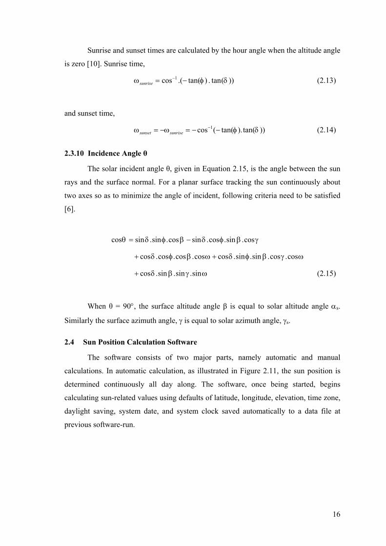
Sunrise and sunset times are calculated by the hour angle when the altitude angle
is zero [10]. Sunrise time,
ω − (2.13) ))( tan. )tan(.(cos 1 δφ= −sunrise
and sunset time,
ω (2.14) ))tan().tan((cos 1 δφω −−=−= −sunrisesunset
2.3.10 Incidence Angle θ
The solar incident angle θ, given in Equation 2.15, is the angle between the sun
rays and the surface normal. For a planar surface tracking the sun continuously about
two axes so as to minimize the angle of incident, following criteria need to be satisfied
[6].
cos γβφδβφδθ cos.sin.cos.sincos.sin.sin −=
ωγβφδωβφδ cos.cos.sin.sin.coscos.cos.cos.cos ++
(2.15) ωγβδ sin.sin.sin.cos+
When θ = 90°, the surface altitude angle β is equal to solar altitude angle αs.
Similarly the surface azimuth angle, γ is equal to solar azimuth angle, γs.
2.4 Sun Position Calculation Software
The software consists of two major parts, namely automatic and manual
calculations. In automatic calculation, as illustrated in Figure 2.11, the sun position is
determined continuously all day along. The software, once being started, begins
calculating sun-related values using defaults of latitude, longitude, elevation, time zone,
daylight saving, system date, and system clock saved automatically to a data file at
previous software-run.
16

Figure 2.11 Automatic calculation Graphical User Interface (GUI)
The calculation is sustained automatically by setting interval time during all day.
If stop button is pressed, automatic calculation will be interrupted. If automatic
calculation button is pressed again, the calculation will continue.
If the prototype is surrounded by geographical objects with higher elevation such
as hills, mountains, etc, the sunrise and sunset may be different from that of the
calculated ones. If such a condition occurs, the height of the highest geographical object
must be entered to the elevation textbox for ending up with reasonable results. Even
when the sunrise and sunset times for locations near the highest object in the world is
calculated, they will only differ slightly compared to those at the sea-level with zero
elevation.
Daylight, time zone, time and date are all set to default computer system values
at the beginning of each software-run. However, if desired otherwise, users may enter
their own new daylight and/or time zone values using the GUI.
Once software is run, most sun-related values are stored into an active Microsoft
Excel sheet concurrently for a possible later use or analysis.
17

Figure 2.12 Manual calculation GUI
The manual part, when desired day and time are accessed to, as shown in
Figure 2.12, can be used to calculate the sun position. The latitude, longitude, time
zone, daylight saving and elevation can be modified as desired.
18

Chapter 3
STRUCTURAL ANALYSIS
3.1 Introduction
Two axis sun tracking system consists of two rotational motions. One of the
motions is deployed to track sun along altitude angle. The other motion, on the other
hand, is employed to track sun along azimuth angle. From this point of view, the
prototype utilizes two motor-gear system pairs.
The prototype, due to natural conditions, is exposed to such disturbances as
wind, rain, and storm. Wind, as the most important disturbance, is taken into
consideration in this thesis.
The prototype is designed to work under statical and dynamical loads due to its
own weight and wind. Prior strength analysis on prototype’s solid model, which is
created in Autodesk Inventor 64, is performed with the help of specific engineering
software. Static analysis is handled in Mechanical Desktop and Autocad Mechanical 64.
Main structure is built using a wood-originated material called as MDF5 because
of its ease of accessibility and material handling. The aluminum, on the other hand, is
utilized as shaft material. The technical characteristics of both materials are shown in
Table 3.1.
Table 3.1 Technical characteristics of MDF and aluminum
Wood (MDF) Aluminum-6061
Thickness 10 mm -
Yield Stress 30 N/mm2 275 N/mm2
Modulus of Elasticity 2500 N/mm2 68900 N/mm2
Ultimate Tensile Stress 0.7 N/mm2 310 N/mm2
Density 800 kg/m3 2710 kg/m3
4 Autodesk Inventor 6, Autocad Mechanical 6, Mechanical Desktop 6 are the official trademark of
Autodesk Inc. 5 MDF stands for Medium Density Fiber board.
19

The main parts of prototype are shown in Figure 3.1.
Figure 3.1 The prototype of two axis sun tracking
20

3.2 Wind Load
Although wind velocity varies with time at the location and is affected by local
topography, the average wind velocity is around 7.03 m/s in IYTE campus area [24].
Wind velocity data collected in IYTE campus area are given in Appendix B. In this
thesis, for the load condition, wind is assumed to be 7 m/s in speed and continuously
parallel to horizon towards north in direction. The wind load is calculated via the basic
equation for flowing gas’s relation between pressure and speed:
2ww V . ρ .
21P = (3.1)
The air density ρ is accepted as constant with a typical value of 1.2 kg/m3 at sea
level. As shown in Figure 3.1, the wind load for Vw ~ 7 m/s wind velocity is,
Pw = ½ * 1.2 * 72 = 29.4 N/m2.
3.3 Static Analysis
3.3.1 Introduction
Static analyses are performed for panel, shaft-1 and shaft-2 of prototype due to
being the most critical components in load exposure. Weight, wind load and motor
torques are included in analyses of each component. Wind load, as aforementioned, is
29.4 N/m2. Component weights are calculated on solid models.
Deflection Line Method and Finite Element Analysis (FEA) are used in bending
moment, stress and deflection analysis of the components. Component dimensions are
updated in accordance with the analysis results.
3.3.2 Panel
Bending moment, stress and deflection on the panel are obtained under wind
load. The biggest wind load on the prototype occurs when the panel stays perpendicular
to the horizon, because of the biggest surface area facing wind.
Load on the panel stems from;
21

• Panel mass = V * ρ = (0.49 * 0.21 * 0.01) * 800 = 0.8232 kg/panel
• Wind load = 0.0000294 N/mm2
As shown in Figure 3.2, the panel has a slight deflection when just wind load
acts on. Exact maximum deflection is 0.04094 mm, as shown in Table 3.2.
Figure 3.2 Deflection analysis result of the panel in FEA
Table 3.2 Maximum panel deflection
22

Bending moment occurred on the panel is figured out as having a value of
0.1569 Nm. Bending moment and deflection distribution graphs6 are illustrated in
Figure 3.3.
Figure 3.3 Resultant deflection line and moment for panel
6 Detailed information can be found in Appendix C.
23

Table 3.3 Maximum stress and maximum bending moment of panel
As depicted in Table 3.3, the maximum stress occurred on the panel is obtained
to be 0.044839 N/mm2. MDF yield stress is known to be 30 N/mm2 based on Table 3.1.
Since the obtained stress value is less than that of allowable value, the panel is safe
under wind load. The panel can be assumed as a rigid body.
3.3.3 Shaft-1
The shaft-1 used to support the panel is considered as shown in Figure 3.1. The
panel is consisting of two parts which are put symmetrically into place facing one
another with 20 mm of equal distance for the system balance. The shaft is supported by
two ball bearings on the derrick of the disc. A pulley on shaft-1 is actuated by a stepper
motor to overcome torque caused by wind load and moment of inertia of panels.
Panel weight is assumed to be linearly distributed.
• Panel’s weight = (2 * 9.81 * 0.8232) / 0.21 = 76.9 N/m (at -z direction)
• Bending moment on panels = 0.1569 Nm (at -y direction)
• The shaft-1 weight = 1.34 * 9.81 = 1.315 N (at -z direction)
• Wind force = 8.62 N (at – x direction)
• Stretch force of belt mechanism = 4.905 N (at -z direction)
24
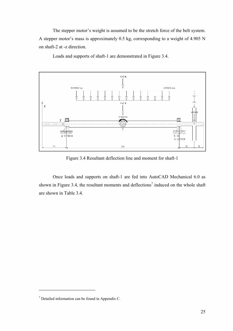
The stepper motor’s weight is assumed to be the stretch force of the belt system.
A stepper motor’s mass is approximately 0.5 kg, corresponding to a weight of 4.905 N
on shaft-2 at -z direction.
Loads and supports of shaft-1 are demonstrated in Figure 3.4.
Figure 3.4 Resultant deflection line and moment for shaft-1
Once loads and supports on shaft-1 are fed into AutoCAD Mechanical 6.0 as
shown in Figure 3.4, the resultant moments and deflections7 induced on the whole shaft
are shown in Table 3.4.
7 Detailed information can be found in Appendix C.
25

Table 3.4 Maximum stress and maximum bending moment of shaft-1
Maximum stress occurred on shaft-1 is 4.3209 N/mm2 as shown in Table 3.4.
Aluminum yield stress is known to be 275 N/mm2 based on Table 3.1. Because obtained
maximum stress value is less than that of allowable value, the shaft-1 is safe under the
loads.
Torsion moment occurred on shaft-1 is found to be 0.166 Nm as shown in Table
3.4, which needs to be compensated by the actuator, namely stepper-1.
3.3.4 Shaft-2
Shaft-2 stays perpendicular to the horizon in the prototype as shown in Figure
3.1. It is supported by two ball bearings on the main case. It has one pulley, driven by
an actuator, namely stepper-2, connected to shaft-2. It needs to be actuated against
moment of inertia of such components as main disc and all others fixed on top of the
disc.
As demonstrated in Figure 3.5, the stepper-1 mounted on the derrick constitutes
a bending moment (Mb) on shaft-2. As aforementioned, average stepper motor weight
as tension of belt mechanism is around 4.905 N. Thus, stepper motor weight on the
derrick of the disc creates bending moment on shaft-2 around -x direction. This bending
moment is calculated utilizing the following formula:
26

Moment = Force * Distance (3.2)
Thus,
Mb = 4.905 * 0.19 = 0.932 Nm
Figure 3.5 Moment acting on shaft-2
Wind load acting on panels and disc surface tries to bend the shaft around -y
(Mw) as shown in Figure 3.5. Bending moment around -y direction is found to be 2.586
Nm.
Mw = 8.62 * 0.3 = 2.586 Nm
As shown in Figure 3.6, the shaft is loaded with disc, derricks, panel, shaft-1 and
stepper-1 weights, which sum up to 36.189 N along -z direction.
27

Loads and supports of shaft-2 are demonstrated in Figure 3.6.
Figure 3.6 Resultant deflection line
and moment for shaft-2
Table 3.5 Maximum stress and maximum
bending moment of shaft-2
Maximum stress occurred on shaft-2 is obtained to be 4.185 N/mm2 as shown in
Table 3.5. Aluminum yield stress has a value of 275 N/mm2 as expressed in Table 3.1.
Hence, obtained maximum stress value is less than that of allowable value; the shaft-2 is
safe under the loads.
28

3.4 Stepper Motor Selection Process
Appropriate stepper motor selection first requires inertia load be determined.
Thus, moment of inertia values for such moving components as the panel and the disc
are automatically calculated as outputs of the solid modeler deployed in this thesis.
Correspondingly, moments of inertia for both components have the values of,
Jpanel= 0.0338 kgm2
Jdisc = 0.04438 kgm2
Maximum angular disc rotation is greater than that of the panel’s. That is why,
stepper motor selection must base on the disc. On 21st June, the disc performs the
biggest angular displacement of approximately ±120 degrees, corresponding to ±2π/3
radians.
For a rigid solid body, the rotational Newton’s Second Law is,
TL = α . Jdisc (3.3)
Estimate α = 9,5 rad/sec2,
TL = 9,5 . 0.04438 = 0.42161 Nm
Desired maximum moment of inertia value is calculated as 0.42 Nm. Owing to
having such a maximum torque need at the load level, both actuators used in the
prototype are selected as 1.8 degree 2 phases unipolar hybrid type 23LM-C355-P6V
series stepper motors made by Minebea Co, Japan.
In the technical characteristics, the stepper motor’s torque is provided as 0.42
Nm. Although selected stepper motors suffice maximum torque need, a reduction ratio
of 4 is preferred so that both the friction load and possible highest wind load can be
overcome. The torque is increased to 1.68 Nm at the load level by a transmission
mechanism. Transmission ratio is,
29

42184
5
7 ===DD
transi (3.4)
Besides, selection of such a transmission ratio results in linearly proportional
resolutions both at the disc and the panel levels.
3.5 System Analysis
3.5.1 Introduction
Mathematical model of the two axis sun tracking system consists of an amplifier,
two stepper motors, belt transmissions and the load. Figure 3.7 depicts simple block
diagram representation of the model.
(s)Θb
StepperMotor
BeltTrasmission
transi1
Panel/DiscPosition
(s)Θm(s)VaLogicSignal Ka GM
Computer Amplifier
(s)Vi
(s)Θd
(s)Θt GL
Θ(s)
GDDisturbance
wV β
Figure 3.7 A simple block diagram of the prototype’s stepper motor mechanism
The transistor is used as an analog amplifier switching from +5 digital logic
voltages to +12 stepper motor supply voltage. The transistor amplification constant is,
4.2Volts 5Volts 12
VVK
i
aa === (3.5)
Belt transmission ratios are determined to be four both for the panel and disc
rotations. The belt transmission ratio is,
411
=transi
(3.6)
30

The disc or panel loads are described by the transfer function GL. This function
includes panel or disc inertia, JL and damping factor, βL.
.sβ.sJ
1(s)Θ
Θ(s)GL
2Lt
L +== (3.7)
Θd is the erroneous angle caused by disturbances such as the wind load acting on
the panel and disc. GD is the transfer function of Θd depending upon disturbance
sources, which will be explained meticulously in upcoming topics.
3.5.2 Mathematical Model of Stepper Motors
Considering the electrical and mechanical characteristics of the system, two
balance equations can be developed when a voltage is applied to stepper motor
windings to initiate the rotor motion.
An equivalent electrical circuit of a stepper motor is illustrated in Figure 3.8
[11]. Voltage source applied across the coils of stator is represented as Vapp. The Vemf is
the induced voltage opposing the voltage source. The induced voltage is often referred
to as the back electromotive-force (EMF).
DC i
R L
TmVapp
mθ
mm β ,JVemf
Figure 3.8 A stepper motor schematic diagram
A differential equation of the equivalent circuit around the electrical loop is
derived from Kirchoff’s voltage law. Kirchoff’s voltage law states that the sum of all
voltages around a loop must equal to zero,
(3.8) 0VVVV emfLRapp =−−−
31

The effect of the back electromotive-force is the feedback signal, which is
proportional to the speed of the stepper motor by coefficient Kb. The field current is
related to the field voltage by,
dt
(t)d . Kdt
di(t) . Li(t) . R(t)V bappmθ
++= (3.9)
When a stepper motor is warned, an actuation torque occurs on the rotor. The
torque induced by the stepper motor is expressed as,
i(t) . K(t)T tm = (3.10)
When the torque is induced by the stepper motor, the resistance torque Tr(t)
occurs. The resistance torque is described by a linear expression proportional to the
speed of rotation of the prototype,
(t)θ . K(t)T mrr = (3.11)
The motor torque Tm(t) is shared by the load and the resistance torque,
Tm(t) = TL(t) + Tr(t) (3.12)
Using Equation 3.10, 3.11 and 3.12, the load torque represented by TL(t)
becomes,
(t)θ . Ki(t) . K(t)T mrtL −= (3.13)
The load torque for rotational inertia can also be written in the form of,
32

dt
(t)d . βdt
(t)θd . J(t)T m2m
2
mLmθ
+= (3.14)
All initial conditions are assumed to be zero. When Laplace Transforms of
Equation 3.9, 3.13 and 3.14 are taken,
(s). .sK L.s).i(s) R((s)V ba mΘ++= (3.15)
(3.16) (s) . Ki(s) . K(s)T rtL mΘ−=
(3.17) (s) β.s).s . J((s)T 2L mΘ+=
are obtained.
Considering Vapp(s) as the input and Θm(s) as the output, the block diagram
based on Equations 3.15, 3.16 and 3.17 is illustrated in Figure 3.9 [11].
L.sR1
+ tKmm β.sJ
1+ s
1mω
rK
bK
Tr(s)
Tm(s) TL(s)
i(s)(s) Vapp (s) Θm
Figure 3.9 Stepper motor block diagram
The transfer function of the stepper motor-load combination in this case is,
.s.KK)K.sβ.sL.s).(J(R
K(s)V(s)Θ
tbrm2
m
t
a
m
++++= (3.18)
33

Stepper motor rotates in constant step angles in response to input signals. When
a single step is required, the rotor tends to overshoot and oscillate about its final
position. The actual response to a position command depends on the technical
specifications of the motor as seen in Table 3.6.
Table 3.6 Stepper motor data list provided by Minebea Co.Ltd.
Kb = 0.035 Volts. sec / rad Vapp = 12 Volts
Kr = 1.05 N.m / rad R = 10 Ohms
Kt = 0.35 N.m /Amp L = 2.5 10-3 H
Jm = 0.11 10-4 kg.m2 βm 0.001 Nm.sec
The block diagram given in Figure 3.9 is used as the basis for a simulation
model in Matlab/Simulink, where a single step response is computed using stepper
motor data, to illustrate the dynamics of the stepper motor, as shown in Figure 3.10.
Figure 3.10 Single step response
34

The single step response of rotor position often exhibits damped oscillations
prior to reaching steady state position angle, (1.8˚). The natural frequency ωn, and
damping ratio ξ of the motor characterize the single step response.
Figure 3.11 The damping ratio ξ and natural frequency ωn
The natural frequency and damping ratio are obtained as ωn =321 rad/sec and
ξ = 0.323 in Matlab, respectively. Ttm, time constant is obtained as 0.0096 sec from
Equation 3.17.
ξ . ω
1Tn
tm = (3.19)
The settling time corresponding to a ±2% or ±5% tolerance band is,
= 4.T2%±st tm =0.0384 sec.
= 3.T5%±st tm =0.0288 sec.
If the stepper motor is driven half step sequence which is 0.9 degree step angle,
Kr resistance constant is divided by two. The single step response of rotor position often
exhibits damped oscillations prior to reaching steady state position angle, (0.9˚). The
single step response for half step angle is shown in Figure 3.12.
35

Figure 3.12 Single step response for half step angle
As shown in Figure 3.12, the settling time for half step angle is 0.0373
corresponding to a ±2% band width. The natural frequency ωn and damping ratio ξ are
obtained 454 rad/sec and 0.228 respectively, as shown in Figure 3.13.
Figure 3.13 The damping ratio ξ and natural frequency ωnf for half step angle
36

3.5.3 Disturbance Effect
The wind load is determined by wind velocity expressed in Equation 3.1, which
was,
Pw = ½ . ρ . Vw 2
The panel or disc is assumed to be rigid under a constituted distributed force
caused by the wind load. Total force acting on the panel due to wind load is,
F = Pw . A (3.18)
V = 7 (m/s)
F (N)
F (N)
Pw (N
/m^2
) γ
Figure 3.14 Schematic panel illustration
Since center of rotation of the panel overlaps with that of shaft-1, the panel area
can be stated as A/2. If distributed force is converted to an equivalent force, the force
acted on a half panel area becomes,
)sin . 2h . w. PF β(= (3.19)
37

Since the equivalent force acts on half of the panel at two thirds of the semi-
height, the torque equals to,
32 .
2h . FTd = (3.20)
If the torque given by Equation 3.20 is reduced,
)sin( .V . h . w. ρ . 121T 22
d β= (3.21)
Disturbance effect is illustrated in Figure 3.15 Kw can be expressed as a
constant.
ρ .h .A . 121Kw = (3.22)
Final format of the disturbance effect for the panel can be written
)sin( .V . K . J.s1 2
w2d β=θ (3.23)
Figure 3.15 Disturbance effect component
As shown in Figure 3.15, the slider gain adjusts to moment effect created by
wind on the panel.
38
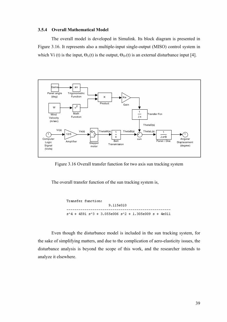
3.5.4 Overall Mathematical Model
The overall model is developed in Simulink. Its block diagram is presented in
Figure 3.16. It represents also a multiple-input single-output (MISO) control system in
which Vi (t) is the input, ΘL(t) is the output, ΘD (t) is an external disturbance input [4].
ThetaD(s)
ThetaL(s)ThetaB(s)Va(s) ThetaM(s)Vi(s)1
AngularDisplacement
(degree)
W
Wind Velocity(m/sec)
sin
TrigonometricFunction
1
J.sTransfer Fcn
sum
Steppermotor
Product
Gama
Panel angle(deg)
1
J.s+BPanel / Disc
u2
MathFunction
Kw
Gain
1
4Belt
Transmission
12/5
Amplifier
1
ComputerLogicSignal(Volts)
Figure 3.16 Overall transfer function for two axis sun tracking system
The overall transfer function of the sun tracking system is,
Even though the disturbance model is included in the sun tracking system, for
the sake of simplifying matters, and due to the complication of aero-elasticity issues, the
disturbance analysis is beyond the scope of this work, and the researcher intends to
analyze it elsewhere.
39
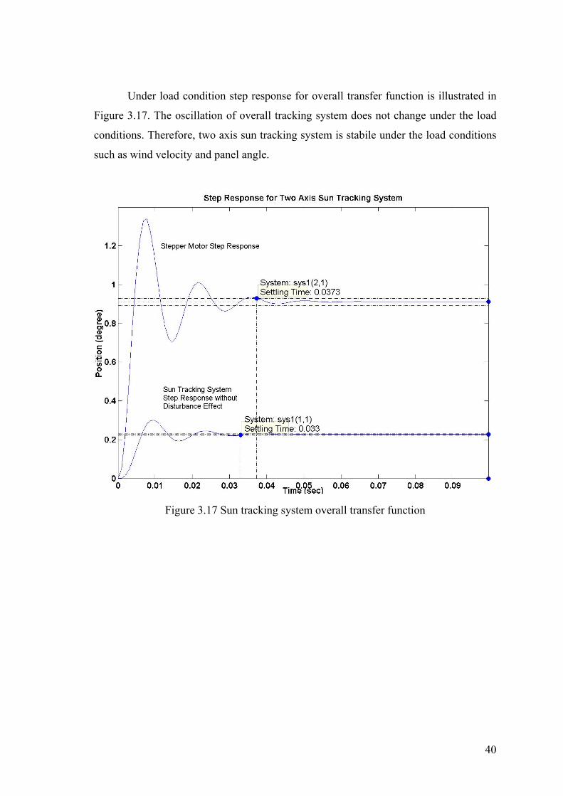
Under load condition step response for overall transfer function is illustrated in
Figure 3.17. The oscillation of overall tracking system does not change under the load
conditions. Therefore, two axis sun tracking system is stabile under the load conditions
such as wind velocity and panel angle.
Figure 3.17 Sun tracking system overall transfer function
40

Chapter 4
ACTUATORS AND CONTROL SYSTEM
4.1 Introduction
The sun’s displacement is very slow. Since the prototype is designed to track the
sun all along the day, the prototype is not needed to have fast rotation capability about
its actuators’ axes. Thus, stepper motors, which provide precise displacement feature
with proportionally low speed, are used for the prototype’s rotational movements.
Stepper motor control, meanwhile, as depicted in Figure 4.1, is performed by the
stepper motor control software and control board developed. The computer control
software generates step pulse signals for the motors. The step pulse signals under
software control include step modes and motor direction. The computer sends
commands to the control board using a direct parallel port connection. The control
board converts the computer commands into the power necessary to energize the motor
windings.
Figure 4.1 Flow diagram
41
4.2 Stepper Motor
4.2.1 Stepper Motor Basics
4.2.1.1 Introduction
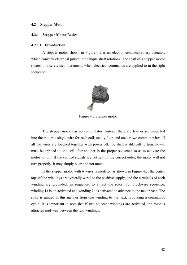
A stepper motor shown in Figure 4.2 is an electromechanical rotary actuator,
which converts electrical pulses into unique shaft rotations. The shaft of a stepper motor
rotates in discrete step increments when electrical commands are applied to in the right
sequence.
Figure 4.2 Stepper motor
The stepper motor has no commutator. Instead, there are five or six wires fed
into the motor: a single wire for each coil, totally four, and one or two common wires. If
all the wires are touched together with power off, the shaft is difficult to turn. Power
must be applied to one coil after another in the proper sequence so as to activate the
motor to turn. If the control signals are not sent in the correct order, the motor will not
turn properly. It may simply buzz and not move.
If the stepper motor with 6 wires is modeled as shown in Figure 4.3, the center
taps of the windings are typically wired to the positive supply, and the terminals of each
winding are grounded, in sequence, to attract the rotor. For clockwise sequence,
winding 1a is de-activated and winding 2a is activated to advance to the next phase. The
rotor is guided in this manner from one winding to the next, producing a continuous
cycle. It is important to note that if two adjacent windings are activated, the rotor is
attracted mid-way between the two windings.
42

Figure 4.3 Conceptual diagram of two-phases
The stepper motor can be controlled digitally with extreme accuracy because of
the fact that stepper motors have non-accumulative rotational error. This means that the
number of rotations that the motor turns can be accurately controlled and measured.
4.2.1.2 Direction and Speed
Sequence of the pulses is directly proportional to the direction of motor shaft
rotation. Reversing the order of the sequence will cause the motor to rotate the other
way. Each pulse equals to one rotary increment, or step, which is only a portion of one
complete rotation. For each pulse or step input, the stepper motor rotates a fixed angular
increment: typically 90, 45, 18, 7.5 or 1.8 degrees.
The speed of the motor shaft rotation is directly proportional to the frequency of
the input pulses and the length of rotation is directly proportional to the number of input
pulses applied. A desired amount of shaft rotation can be achieved by pulse counting.
4.2.1.3 Torque
Induced torque versus angular displacement of the motor curve demonstrates a
sinusoidal change as shown in Figure 4.4. As long as the torque remains below the
holding torque of the motor, the rotor will remain within ¼ period of the equilibrium
position. This implies that a stepper motor will be within one step of the equilibrium
position. This can be useful for applications where the motor may be starting or
stopping, while the force acting against the motor remains present. In order to achieve
43

this equilibrium, every time an electrical pulse is sent to the motor, the motor steps
once.
Figure 4.4 The torque period versus position curve [33]
Once the motor takes a step, the available torque is at a minimum, which
determines the running torque when the rotor is half way from one step to the next, as
shown in Figure 4.5. For the maximum torque, the motor can drive as it steps forward
slowly. At higher stepping speeds, the running torque is sometimes defined as the pull-
out torque. Pull-out torque is the dynamic torque that the motor can sustain in the same
direction with integrity.
Figure 4.5 Stepper motor torque vs. angular displacement [33]
With no power to any of the motor windings, the torque does not always fall to
zero. The combination of pole geometry and the permanently magnetized rotor may
lead to significant torque with no applied power. The residual torque is frequently called
detent torque. The most common motor designs yield a detent torque that varies
sinusoidal with rotor angle, with an equilibrium position at every step and amplitude of
roughly 10-20% of the rated holding torque of the motor.
44

4.2.1.4 Resonance
The resonance problem can be seen as a sudden loss or drop in torque at certain
speeds, which can result in, missed steps or loss of synchronism. It occurs when the
input step pulse rate coincides with the natural oscillation frequency of the rotor. Often
there is a resonance area around the 70-120 steps per second region and also one in the
high step pulse rate region. [33] The resonance of motor is also dependent upon the load
conditions and is not possible to be eliminated completely.
Elastomeric couplings are utilized as belt systems between stepper motors and
loads in the prototype, since they provide avoidance of resonation problems. In addition,
as will be expressed later, having selected half phase excitation driving mode, resonance
problem is decreased to the minimum level.
4.2.2 Stepper Motor Types
There are three basic stepper motor types [35]:
• The variable-reluctance motor,
• The permanent-magnet motor,
• The hybrid motor.
Variable-reluctance stepper motors consist of a soft iron multi-toothed rotor and
a wound stator. The rotor spins freely without any detent torque. When the stator
windings are energized with DC current, the poles become magnetized. Rotation occurs
when the rotor teeth are attracted to the energized stator poles. This type of motor is
frequently used in small applications such as micro-positioning.
Permanent-magnet motors are perhaps the most widely used type in non-
industrial applications. This motor has toothless rotor and is magnetized with alternating
north and south poles of the permanent magnet. It is a low-cost, low-torque, low-speed
device ideally suited to applications, such as computer peripherals.
Hybrid motors combine the best characteristics of the variable reluctance and
permanent magnet motors. They have high detent torque and excellent holding and
running torque, and they can operate at high stepping speeds. As shown in Figure 4.6,
they are constructed with multi-toothed stator poles and a permanent magnet rotor.
Standard hybrid motors have 200 rotor teeth and rotate at 1.8-degree step angles. This
45

motor can also be driven two phases at a time to yield more torque, or alternately one
then two then one phase, to produce half steps or 0.9-degree increments. Hybrid motors
are used in a wide variety of industrial applications.
Figure 4.6 Hybrid stepper motor
4.2.3 Stepper Motor Selection
Some criteria are taken into consideration to determine the stepper motors used
in the prototype can be listed as:
• High-resolution ratio: because wide range of angular orientation must be
supported.
• High positioning accuracy: because precise displacement is desired in open-loop
control.
• Low power consumption: because overall efficiency of the system is to be
maximized.
• High detent and holding torque; because the prototype works against wind load.
Two standard hybrid stepper motors by Minebea Co. Ltd. Type 23LM-C355-
P6V rotating 1.8 degrees for every full step and having 200 poles are used in the
prototype.
Furthermore, in order to increase the resolution of the rotational system by
transmission ratio, belt systems are employed in the prototype. Thus, owing to
46

transmission ratios of 4 and half phase step excitation mode, when each stepper motor
rotates 360 degrees, 45 degrees of the panel and disc rotation is obtained.
Due to not having a closed loop positioning mechanism, accurate rotational
movements at the motor outputs are vital. The motors deployed in the prototype
guarantee step accuracy error less than five percent. Since the angular output resolution
of the motors are 1.8 degrees, a maximum of five-percent positional accuracy yields
0.09 degrees of error per step [26].
Motors employed in the prototype pull a current of 1.2 Amp at 12 Volt DC only
when they are under load. Overall run-hours of the prototype depend upon user’s track
sensitivity selection and day length.
In addition to having high detent and excellent holding torque, they are good at
high stepping speeds as well. The detent torque and shortcut of all stepper wires when
the power is off together resist rotor to rotate. Such a resistance, thus, eliminates the
need for an external mechanical brake mechanism.
4.2.4 Stepper Motor Driving Modes
There are two commonly used excitation modes; full-step and half-step to drive
stepper motors. In full step operation, the motor steps through the normal step angle, for
instance, it takes 1.8 degree/step in 200 step/revolution motors. There are two kinds of
full-step modes, single phase and dual phase excitation.
In single phase full-step excitation, the motor is operated with only one phase
energized at-a-time. The stepper motor torque and speed performances are not good,
and problems with resonance can preclude operation at some speeds.
In dual phase full-step excitation, whereas, the motor is operated with two
phases’ energized at-a-time. This mode provides good torque and speed performance
with minimum resonance problems, but it does require twice the power of that of single
phase.
Half-step excitation is an alternative to single and dual phase operation resulting
in steps one half that of normal step sizes. This mode provides twice the resolution. In
the half step modes, the step angle is 0.9 degree, corresponding to 400 steps per
revolution for standard hybrid stepper motor. This mode offers almost complete escape
from resonance problems. In this mode, motors can be operated over a wide range of
speeds and used to drive almost any load commonly encountered.
47

4.2.5 Stepper Motor Driving Mode Selection
Because of resonance problem at specific speeds, single phase full-step
excitation is not preferred to drive stepper motors on the prototype. Dual excitation
provides about 30 to 40 percent higher torque than that of single-phase excitation.
However, because twice the power is required from the power supply, dual excitation is
not chosen to drive stepper motors. Due to providing twice resolution, avoidance of
resonance problem and good torque speed characteristics, half step excitation is
preferred to drive stepper motors.
Based on stepper motor wires numbering format as Figure 4.6, Table 4.1 details
half-step driving sequence:
Table 4.1 Half-step excitation sequence
Step 1 2 3 4 5 6 7 8
A 1 1 0 0 0 0 0 1
B 0 1 1 1 0 0 0 0
C 0 0 0 1 1 1 0 0
D 0 0 0 0 0 1 1 1
4.3 Sensors
4.3.1 Reference Sensors
Four reference sensors are used in the prototype. One of them is placed on the
prototype body to indicate south direction at a fixed point on the disc. Two other
sensors placed on the body ensure that the disc heads to reference point using the
shortest way as well. The last reference sensor is, unlike the first three, fixed on the disc
so as to serve as the reference point of the panel. First and last sensors aim to determine
start and stop point of the stepper motors. The sensors send four-bit feedback signal to
control software via parallel port. Each of these reference sensors can be eliminated by a
hand switch on the control board.
48
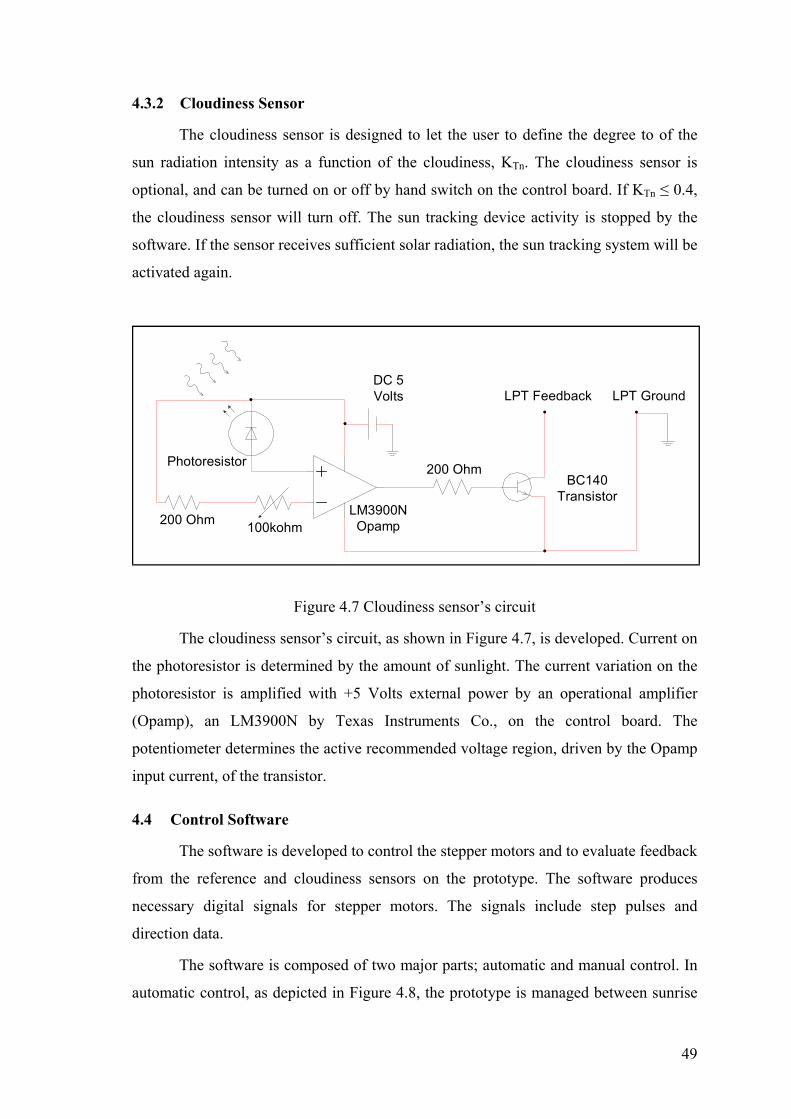
4.3.2 Cloudiness Sensor
The cloudiness sensor is designed to let the user to define the degree to of the
sun radiation intensity as a function of the cloudiness, KTn. The cloudiness sensor is
optional, and can be turned on or off by hand switch on the control board. If KTn ≤ 0.4,
the cloudiness sensor will turn off. The sun tracking device activity is stopped by the
software. If the sensor receives sufficient solar radiation, the sun tracking system will be
activated again.
LM3900NOpamp
BC140Transistor
DC 5Volts LPT Feedback LPT Ground
100kohm
Photoresistor
200 Ohm
200 Ohm
Figure 4.7 Cloudiness sensor’s circuit
The cloudiness sensor’s circuit, as shown in Figure 4.7, is developed. Current on
the photoresistor is determined by the amount of sunlight. The current variation on the
photoresistor is amplified with +5 Volts external power by an operational amplifier
(Opamp), an LM3900N by Texas Instruments Co., on the control board. The
potentiometer determines the active recommended voltage region, driven by the Opamp
input current, of the transistor.
4.4 Control Software
The software is developed to control the stepper motors and to evaluate feedback
from the reference and cloudiness sensors on the prototype. The software produces
necessary digital signals for stepper motors. The signals include step pulses and
direction data.
The software is composed of two major parts; automatic and manual control. In
automatic control, as depicted in Figure 4.8, the prototype is managed between sunrise
49

and sunset. When start button is pressed, the motors go to the reference points. After
three seconds, if at least one of altitude and azimuth angles is different from zero, panel
and disc rotate to corresponding altitude and azimuth angles respectively.
The minimum angular difference between at least one of the calculated altitude
and panel angle, or azimuth angle and disc angle pairs is called Tracking Sensitivity.
After panel and disc reach to the desired azimuth and altitude angles, the next group of
motions will take place only if user-defined Tracking Sensitivity condition is satisfied.
Figure 4.8 Automatic Control Graphical User Interface (GUI)
As shown in Figure 4.9, the stepper motors can be rotated separately at desired
direction in manual control part. The stepper motors’ velocity can be set via delay time
slider control in the graphical user interface. Delay time states time elapsed between
two digital step signals.
When user enters desired steps or angle of rotation, the corresponding panel or
disc rotates based on input parameters. Thus, the magnitude of rotation and direction are
achieved. If the reference point command is entered, the panel or disc rotates to its
respective fixed reference point.
50

When brake checkbox is enabled, immediately after power turn off, all stepper
motor wires are shortcut to lock motor shaft. This event increase brake ratio supported
by the stepper motor’s detent torque.
Figure 4.9 Manual Control GUI
Control software is developed in Visual Basic 6.01 editor [12], [15]. The stepper motor
sequences and reference point inputs are arranged in Visual Basic editor as well.
Communication between parallel port and computer is directly possible under Windows
95/98/Me8 operating systems (OS), but it is not supported under Windows NT-based
OS’s. To overcome the problem in NT-based OS’s, the DriverLINX9 parallel port driver
is used.
8 Windows 95/98/Me, Windows NT/2000/XP, and Visual Basic are registered trademarks
of Microsoft Corporation. 9 DriverLINX is a registered trademark of Scientific Software Tools, Inc.
51

4.5 Parallel Port
The computer is a common IBM10-compatible PC. Every PC has at least one
parallel port. IBM designed PC parallel port adapter specifically to attach printers with a
parallel port interface, but it can be used as a general input/output (I/O) port for any
device or application that matches its I/O capabilities.
The parallel port output is normally at TTL11 voltage levels. As shown in Figure
4.10, they put out ideally 0 Volt when they are in low logic level (Binary 0) and +5
Volts when they are in high logic level (Binary 1). The parallel port current capacity is
limited to only few milliamperes per pin such that sink and source currents vary around
12 mA. Some of the pins are inverted by the parallel port card. If +5 Volts (Logic 1)
was applied to inverted pin, for instance, it would return back a 0 Volt (Logic 0), vice
versa.
Figure 4.10 Parallel Port logic levels
The parallel port is made up of three different sections. These are the data lines,
control lines and status lines. The original IBM standard DB25-based parallel output
port schematic diagram is shown in Figure 4.11.
Figure 4.11 The parallel port standard DB25 interface [36].
10 International Business Machines Corporation. 11 Transistor-Transistor Logic
52

• 8 output pins accessed via data lines D0-D7
• 5 input pins (one inverted) accessed via status lines S3-S7
• 4 output pins (three inverted) accessed via control lines C0-C3
• The remaining 8 pins are grounded (18-25)
Many PC has single parallel ports integrated to the motherboard and they are
normally assigned 378h base address in hexadecimal code. If a second parallel port is
available in PC, 278h base address in hexadecimal code is assigned. These addresses
may change from machine to machine. In this thesis, control software talks through
parallel port coded with 378h base address. However, for all computers, the parallel port
base address can easily be changed in computer’s BIOS12 setup.
For the 378h base address, each parallel port section is accessed by its own
address and will act independently from the rest. As shown in Table 4.2, the addresses
can be decimal or hexadecimal format.
Table 4.2 Standard Parallel Port Addresses
Port Address (Decimal) Address (Hexadecimal)
Data Lines (Base) 888 378h
Status Lines(Base + 1) 889 379h
Control Lines (Base + 2) 890 37Ah
The data communication between the computer and the prototype is handled via
parallel port. The parallel port’s eight-bit data lines, as shown in Table 4.3, are shared
as: four-bit for stepper motor-1 (D0, D1, D2, and D3), and four-bit for stepper motor-2
(D4, D5, D6, and D7). Each pin is capable of sourcing and sinking 12 mA, and can
supply +5 Volts. These current and voltage levels are not enough to feed the stepper
motor coils, thus control board with transistors to amplify the current and voltage is
developed.
12 Basic Input/Output System.
53

Table 4.3 Data Lines
Address Utilize Bit No. Properties Pin No
Bit 0 D0 2
Bit 1 D1 3
Bit 2 D2 4
Stepper
Motor-1
Bit 3 D3 5
Bit 4 D4 6
Bit 5 D5 7
Bit 6 D6 8
&378h
(888)
Stepper
Motor-2
Bit 7 D7 9
The five-bit digital signal of status lines is read to the computer from the input
pins numbered as 10, 11, 12, 13, and 15, shown in Table 4.4. The S3 status line is
utilized to connect cloudiness sensor. S4 status port line describes reference point-4,
which is used for the disc on the prototype, and S7 status port line describes reference
point-1, which is used for the panel. Meanwhile, S5 and S6 status port lines refer to the
reference point-2 and reference point-3, which are used to sense disc’s lower and upper
rotational limits. Thus, the panel and disc positions are determined. Only once the lines
are touched to LPT ground, the input signals transmit a Logic 1 level input signal to
computer.
Table 4.4 Status Lines
Address Utilize Bit No. Properties Pin No.
Cloudiness Sensor Bit 3 S3 15
Reference Point-1 Bit 4 S4 13
Reference Point-2 Bit 5 S5 12
Reference Point-3 Bit 6 S6 10
&379h
(889)
Reference Point-4 Bit 7 S7 11
54

To handle brake function of the prototype, all stepper motor wires are shortcut
when power is off. Two out of four control lines, shown in Table 4.5, are used to control
stepper motor brake systems. C2 control line is used to control stepper motor-1 brake
system. C3 control line is used to control stepper motor-2 brake system.
Table 4.5 Control Lines
Address Utilize Bit No. Properties Pin No.
- Bit 0 C0 1
- Bit 1 C1 14
Brake-1 Bit 2 C2 16
&37Ah
(890)
Brake-2 Bit 3 C3 17
4.6 Control Board
The digital control signals from PC’s parallel port do not have sufficient power
to run stepper motors in the prototype. That’s why a control board is developed to
amplify the digital signals to sufficient levels of current and voltage. The control board
also operates two brake systems and running/stopping signals. Also this control board is
utilized to transmit input signals received from the reference switches and cloudiness
sensor. The control board’s electronic circuit diagram for a single stepper motor is
depicted in Figure 4.12.
In control of stepper motors with parallel port signals, parallel port must get
isolated from the stepper motors’ wires. Since the stepper motor coils have a large
amount of inductance, when the current is cut off they generate a very high-level of
voltage spike. Use of optical isolation devices such as Motorola 4N25 optoisolators will
protect between the delicate control logic and the high-voltage potentials in the power
output stage. As shown in Figure 4.13, the 4N25 optoisolator includes an infrared
emitting diode and a phototransistor pair. When the infrared diode is warned by the
parallel port’s digital signal produced by the software, the phototransistor current flows
from collector (5) to emitter (4).
55

4N25
100 Ohm
4N25100 Ohm
Relay CY-12V
Optoisolator
Optoisolator
TIP 141F
TIP 141F
1000 Ohm
1000 Ohm
12V Dc
5V Dc
5V Dc
12V Dc
BD 135
D2
D3
4N25
100 Ohm
4N25100 Ohm
Relay CY-12VOptoisolator
Optoisolator
TIP 141F
TIP 141F
1000 Ohm
1000 Ohm
12V Dc
5V Dc
5V Dc
12V Dc
BD 135
D0
D1
C2
STEPPER MOTOR
Figure 4.12 Electronic Circuit
Figure 4.13 Motorola 4N25 Optoisolator
56

The stepper motors work with +12 Volt DC and 1.2 Amp current. This power is
fed by external power supply.
Each of the four parallel port output lines (D0, D1, D2, and D3) are used to
switch a Fairchild TIP 141F NPN type Darlington transistor controlling a coil in the
motor. Emitter-collector currents of such transistors work well with continuous 10
Amperes without heating. Thus, heat sink need gets eliminated.
Optoisolator’s emitter polarizes the transistor’s base pin. The transistors are
protected from excessive current flow by 1 Kohm resistors.
Shortcut of motor wires for brake mechanisms’ activation is realized with the
help of four 12-volt relays on the control board. Each relay, as shown in Figure 4.12,
can be used to shortcut only two coils. Since each motor has four coils, use of two
relays per motor becomes a must. Hence, the prototype requires use of four relays
totally.
Each motor is controlled by an input signal amplified beforehand by a BC 135
transistor, which is fed into two relays. Each relay, when brake signal is not activated,
also serves as signal transmission path from parallel port to corresponding motor. Thus,
two out of four relay outputs are reserved to motor coil signal transmission, whereas the
other two are deployed for brake mechanism. Again, two of four relay inputs are used
for motor input signal connections, and the rest are utilized for relay solenoid activation.
Such a flexible electronic structure lets control software to activate motor control signal
transmission while disabling the brake mechanism, vice versa. Each motor or brake
mechanism can be eliminated by a hand switch on the control board as well.
The digital step sequence signals can be seen by the red led diode on the control
board. Besides, brake signals can be distinguished by the green and yellow led diodes
on the control board. Since these led diodes have very low-level of resistance, they are
protected with the help of 100 Ohms of pre-resistances.
57

Chapter 5
RESULTS AND DISCUSSION
Evaluation of the prototype performing two-axis sun tracking based on net
energy production is needed so as to justify the thesis that continuous sun tracking
would end up with higher levels of energy gain compared to that of a fixed counterpart.
For the sake of energy production versus energy consumption of the prototype, each
energy term must be included specifically. While beam radiation plays the key role in
energy production on photovoltaic cells, power of the motors as prototype actuators is
the source of energy consumption. Once each term is unveiled one by one, only then
efficiency of the system and energy justification of the prototype can be resolved.
Below are the steps towards this purpose.
5.1 Beam Radiation Acting on a Surface
The radiation emitted by the sun, and its spatial relationship to the earth result in
a nearly fixed intensity of solar radiation outside the earth atmosphere. The solar
constant, Gsc, is the energy of the sun per unit time received on a unit area of a surface
perpendicular to the direction of radiation propagation at mean earth-sun distance
outside the atmosphere. For solar constant, Gsc, value is assumed to be 1353 W/m2,
which was also approved by NASA [6].
The solar radiation incident on a horizontal plane outside the atmosphere is the
normal incident extraterrestrial solar radiation, named as Gon.
+=
365.360cos.033.01. m
sconNGG (5.1)
The radiation on the tilted surface was considered in Section 2.2.1 to include
three types of components: beam, diffuse, and reflected. Since eighty-percent of the
total sun radiation is caused by the beam type [9], diffuse and reflected radiations can be
included into the beam radiation, which causes it to be approximately equal to total
solar radiation [6].
58

Gon = Gbn (5.2)
For horizontal surfaces, the incidence angle is the zenith angle of the sun, θz,
which also corresponds to the angle between the horizontal and the line to the sun [6].
In this situation, β = 0˚, γ = 0˚, and therefore, Equation 2.15 becomes,
(5.3) δφωδφθ sin.sincos.cos.coscos +=z
Figure 5.1 indicates the angle of incidence of beam radiation on the horizontal
and tilted surfaces.
Figure 5.1 Beam radiation on horizontal and tilted surfaces.
For horizontal surfaces, beam radiation is,
Gb = Gbn . cos θz (5.4)
For tilted surfaces, however, beam radiation is,
Gbt = Gbn . cos θ (5.5)
59

5.2 Energy Production versus Consumption
Since photovoltaic arrays offer very limited levels of efficiency, they can
harness only a minor portion of the beam radiation in the production of electrical
energy. Because a candidate photovoltaic array meeting the prototype specifications
such as Uni-Solar type OST-5 as listed in Appendix E, offer an efficiency value of
4.84%, the difference in between the energy production versus consumption is not that
clear. Being aware of this fact, energy production on photovoltaic arrays and
consumption of the stepper motors are stated as follows,
Energy production on photovoltaic arrays,
Pproduction = A . η . Gbt . t [Wh] (5.6)
The average photovoltaic efficiency from beam radiation at standard test
conditions of 1000 W/m2 irradiance to electricity production, η can be calculated as,
bt
operationoperation
G .A I . V
η = (5.7)
0481,01000 . )(0,49.0,21
0,30 . 16,5η ==
Stepper motor energy consumption,
Pconsumption = Vapp . i . t [Wh] (5.8)
5.3 Optimum Tracking Frequency for Maximum Energy Gain
Under optimum operating conditions and based on extraterrestrial solar
radiation; fixed and tracker type photovoltaic arrays are theoretically compared based
upon the energy efficacy as in preceding equations. 3.6 degree tracking sensitivity value
is evaluated for the tracker type photovoltaic array in average day of the months [3].
Under optimum operating conditions for fixed type photovoltaic arrays,
60

• The slope angle is equal to site’s latitude, β = 38˚, and surface azimuth angle is
γ = 0˚,
whereas in tracker type photovoltaic arrays,
• β and γ are determined depending on tracking sensitivity value of 3.6 degree.
With the help of the sun position calculation software, altitude and azimuth
angles are determined in four-minute time intervals. Beam radiation acting on fixed and
tracker type photovoltaic array surfaces are calculated, and automatically transferred to
MS-Excel spreadsheets for energy-based photovoltaic array justification analysis. The
result of the comparison is shown in Figure 5.2 in the form of excel chart for the
average day of the month. Thus, average annual energy gain for fixed and two-axis sun
tracking photovoltaic systems are obtained theoretically.
Annual Energy Diagram
0
10
20
30
40
50
60
70
80
90
100
17-Jan-2002
16-Feb-2002
15-Mar-2002
15-Apr-2002
15-May-2002
11-Jun-2002
17-Jul-2002
16-Aug-2002
15-Sep-2002
15-Oct-2002
14-Nov-2002
10-Dec-2002
Monthly average daily radiation
Ener
gy (
Wh
)
Two-axis Sun Tracking System Self Consumption of Sun Tracking SystemNet Energy Gain of Sun Tracking System Net Energy Gain of South Facing Fixed System
Figure 5.2 Energy Gain Comparison of fixed and two-axis sun tracking systems
61

Figure 5.2, nevertheless, approved the fact that a two-axis sun tracking system
causes a major jump in overall system performance compared to that of a fixed one in
60 percent levels. Such an increase in the energy gain, as the thesis of this study claims,
provides sufficient proof of data to confirm the fact that sun tracking would result in
inevitable energy gain.
Annual Energy Diagram
0.00
10.00
20.00
30.00
40.00
50.00
60.00
70.00
17-Jan-2002
16-Feb-2002
15-Mar-2002
15-Apr-2002
15-May-2002
11-Jun-2002
17-Jul-2002
16-Aug-2002
15-Sep-2002
15-Oct-2002
14-Nov-2002
10-Dec-2002
Monthly average daily radiation
Harvested Net Energy by Sun Tracking System / Harvested Net Energy by Fixed SystemAnnual Average Efficiency
Figure 5.3 Net Energy Gain
If energy dissipation of the stepper motors of the prototype is subtracted from
the overall energy gain values of the two-axis sun tracking system, harvested net energy
gain is obtained. Therefore, net energy gain relative to that of an identical fixed system
is obtained to be about 40 percent as shown in Figure 5.3.
62

Chapter 6
CONCLUSIONS
A prototype similar to a two degrees of freedom gyroscope is designed, and then
its performance is investigated during the track of the sun via a two-axis open loop
computer control. The prototype is controlled by astronomical equations encoded into
the software. A control board as an interface in between the prototype and computer
using LPT port is designed and manufactured. The prototype is also analyzed in CAD
and CAE against such loads as inertia and wind. The mathematical model is generated
in Matlab/Simulink as well.
Open loop control strategy is deployed in this thesis, which requires a precise
installation of collectors, regarding both the orientation of the structure and the correct
mounting of the reference sensors. Therefore, if pre-requisites are accomplished
satisfactorily, then open loop solar tracking can be used, as in this thesis.
Performance of a two-axis sun tracking system is compared with an identical
fixed system facing southwards with a surface tilt angle equal to the site’s latitude, 38
degrees in our case. Outcomes of this theoretical comparison study under extraterrestrial
solar radiation delivered the fact that a two-axis sun tracking system causes a major
increase in overall system performance in about 40 percent levels compared to that of a
fixed one.
63

REFERENCES
[1] “The Astronomical Almanac For The Year 2001”, Washington: U.S.
Government Printing Office, 2001.
[2] “The Astronomical Almanac For The Year 2002”, Washington: U.S.
Government Printing Office, 2002.
[3] G. Atagündüz, “Güneş Enerjisi Temelleri ve Uygulamaları”, Ege Üniversitesi
Basımevi, 1989.
[4] J. J. D’azzo, C. H. Houpis, “Linear Control System Analysis and Design”, Mc-
Graw-Hill Book Company, 1995.
[5] R. Dorf, R. H. Bishop, “Modern Control System”, Prentice Hall, 2001.
[6] J.A. Duffie, and W.A. Beckman, “Solar Engineering of Thermal Processes”, a
Willey-Interscience Publication, 1991.
[7] J. S. Hsieh, New Jersey Institute of Technology “Solar Energy Engineering”,
Prentice-Hall, 1986.
[8] A. Kızılırmak, “Gökbilim Dersleri, Küresel Bilim”, Cilt 1, Ege Üniversitesi
Basımevi, 1998.
[9] J. F. Kreider, C. J. Hoogendoorn, F. Kreith, “Solar Design Component, System,
Economics”, Hemisphere Publishing Corporation, 1989.
[10] J. Kreider, F. Kreith, “Solar Energy Handbook”, McGraw-Hill Book Company,
1991
[11] T. Özel, “Motion Control and Accuracy Analysis of a Computer Controlled
Model Driving System”, Dokuz Eylül üniversitesi, 1991.
[12] Sybex Yazar Grubu, “Visual Basic 6 Complete”, Alfa Basım, 1999.
[13] Ersoy Taşdemiroğlu, “Solar Energy Utilization; Technical and Economic
Aspects”, Middle East Technical University, 1990.
[14] E. Uyar, “Sistem Dinamiği ve Otomatik Kontrol”, Dokuz Eylül Üniversitesi,
1998.
[15] M. Yanık, “Microsoft Visual Basic 5.0 for Windows 95”, Beta Basım, 1998.
64

[16] H.Yüncü, E. Paykoç, Y. Yener, “Solar Energy Utilization”, Martinus Nijhoff
Publishers, 1987.
[17] “Data irradiation”, 1998,
http://www.anu.edu.au/engn/solar/Sun/Irrad/Irradiation.html.
[18] K. Burnett, “Converting RA and DEC to ALT and AZ”, 2001,
http://www.xylem.f2s.com/kepler/index.html.
[19] P. Drago, Solar Energy, 1978, 20, pp. 419-424.
[20] U.S. Department of Energy Photovoltaics Program “About Photovoltaics”, 2002,
http://www.eren.doe.gov/pv/whyuse.html.
[21] P. Gandhidasan, S. Satcunanathan, “Energy collection augmentation in tracking
flat plate collectors”, Proceedings of Sun World Forum, Brighton, 1981, pp. 186-191.
[22] A. N. Khalifa, S. S. Al-Mutawalli, “Effect of Two-axis Sun Tracking on the
Performance of Compound Parabolic Concentrators”, Energy Convers.Mgmt, Vol. 39,
No.10, pp. 1073-1079, 1998.
[23] B. Koyuncu, K. Balasubramanian, “A Microprocessor Controlled Automatic
Sun Tracker”, IEEE Transactions on Consumer Electronics, Vol.37, No. 4, 1991.
[24] H.M. Türkeli, “An Experimental Investigation of the Parameters to Classify
Wind Sites”, IYTE, 2002
[25] M.A. Mohamad, M.M. Sharaf, N. M. El-Rabaie, “Photovoltaic Sun Tracking
System”, The ISES International Consultants Network (ICN), 1998.
[26] M.Polat, M. Çıbuk, H. Kürüm, “Hibrit Adım Motorlarının İncelenmesi ve
PSICE Benzetimi”, Elektrik-Elektronik Bilgisayar Mühendisliği 9. Ulusal Kongresi,
Kocaeli, 19-23 Eylül 2001, S. 102-105.
[27] S. Satcunanathan, et al., “The design and performance of a semi-tracking flat
plate collector”, Proceedings of Solar World Congress, Perth, 1983, pp. 757-761.
[28] “Sun angle”, http://www.susdesign.com/sunangle/index.html.
[29] Sunlit design “Geography”, 2002,
http://www.sunlitdesign.com/infosearch/geography.htm#longlat.gif.
[30] Dr. J. R. White, “Case Study E-Light Tracking Servo System”, 1997,
http://gershwin.ens.fr/vdaniel/Doc-Locale/Cours-Mirrored/Methodes-Maths/online.htm.
[31] Picture, John Wiley & Sons Inc.
65

[32] D.W.Jones, “Stepper motor types”, 2002,
http://www.cs.uiowa.edu/~jones/step/types.html.
[33] D.W.Jones, “Stepper motor physics”, 2002,
http://www.cs.uiowa.edu/~jones/step/physics.html.
[34] Parker Motion and Control, “Stepper motors”,
http://www.compumotor.com/catalog/catalogA/A04-A11.pdf
[35] S.B.Morrise, “Automated Manufacturing Ststem”, Mc-Graw Hill, 1995.
[36] “IBM-PC Parallel Printer”, 2002
http://www.doc.ic.ac.uk/~ih/doc/par/doc/program.html
66

APPENDIX A
Table A.1 Energy Gain Comparison of fixed and two-axis sun tracking systems based
on the monthly average daily radiation.
Monthly average daily
radiation
Sun Tracking System (STS) (Wh)
Self Consumption
of STS (Wh)
Net Energy Gain of STS
(Wh)
Net Energy Gain of South Facing Fixed
system (Wh)
Efficiency
17-Jan-2002 66.502 6.065 60.437 46.02 31.33
16-Feb-2002 69.841 7.193 62.648 48.35 32.45
15-Mar-2002 78.663 8.377 70.286 51.796 35.70
15-Apr-2002 81.906 9.924 71.982 49.51 45.39
15-May-2002 90.529 11.084 79.445 50.35 57.79
11-Jun-2002 89.458 11.582 77.876 47.537 63.82
17-Jul-2002 94.295 11.490 82.805 51.33 61.32
16-Aug-2002 87.661 10.518 77.142 51.21 50.64
15-Sep-2002 77.66 9.183 68.482 49.767 37.61
15-Oct-2002 75.673 7.578 68.095 51.862 31.30
14-Nov-2002 71.285 6.414 64.87 49.52 31.00
10-Dec-2002 68.981 5.767 63.214 47.6 30.56
A-I

APPENDIX B
Wind distribution on IYTE campus area:
0
1
2
3
4
5
6
7
8
WindSpeed(m/s)
Tem.00 Ağu.00 Eyl.00 Eki.00 Kas.00 Ara.00 Oca.01 Şub.01 Mar.01 Nis.01 May.01 Haz.01 Tem.01 Ağu.01 Eyl.01 Eki.01 Kas.01months
Mean Speed of 10 m
Figure B.1 Variation of monthly mean wind speeds of IYTE campus area at 10 m.
Total mean speed at 10 m is 7.03 m/s [24].
B-I

APPENDIX C
Static analysis for some critical parts of prototype,
For the Panel
Figure C.1 The stress distribution on the panel
C-I
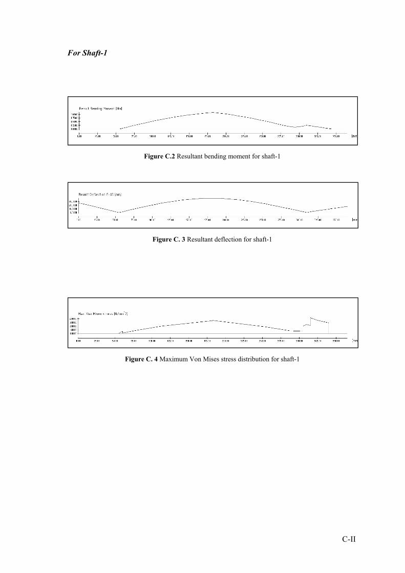
For Shaft-1
Figure C.2 Resultant bending moment for shaft-1
Figure C. 3 Resultant deflection for shaft-1
Figure C. 4 Maximum Von Mises stress distribution for shaft-1
C-II

For Shaft-2
Figure C.5 Maximum bending moment for shaft-2
Figure C.6 Resultant deflection for shaft-2
Figure C.7 Maximum resultant bending stress for shaft-2
Figure C.8 Maximum axial stress for shaft-2
C-III

APPENDIX D
Stepper Motor Technical Characteristics
23 LM- C355-P6V MINI ANGLE STEPPER MOTOR
RATED VOLTAGE 12 V
RATED CURRENT 1.2 A / PHASE
SHAFT DIRECTION BIDIRECTIONAL
TEMPERATURE RISE 80 C MAX
CLASS OF INSULATION BIDIRECTIONAL
STEP ANGLE 1.8 DEG
STEP ACCURACY (SPREAD) 5%
HOLDING TORQUE 4200 g.cm = 0.42 Nm
PULL OUT TORQUE 2500 g-cm Min. AT 4800 PPS
PULL OUT TORQUE 2150 g-cm Min. AT 5600 PPS
MAX SLEW SPEED PPS Min
DETENT TORQUE 0.0850 Nm MAX
DC WINDING RESISTANCE 3.5 + 6.5 OHM ± 10%
WINDING INDUCTANCE 2.5 mH ± 20 %
INSULATION RESISTANCE 100 M OHM Min
DIELECTRIC STRENGTH 500 V AC
ROTOR INERTIA 110 gcm² = 0.11 kgcm²
WEIGHT 550 gr
VIBRATION 2G MAX / 1111, 4800 PPS)
Kb 0.035 VOLTS. SEC /RAD
Kr 1.05 Nm / RAD
Kt 0.35 Nm / AMP
D-I
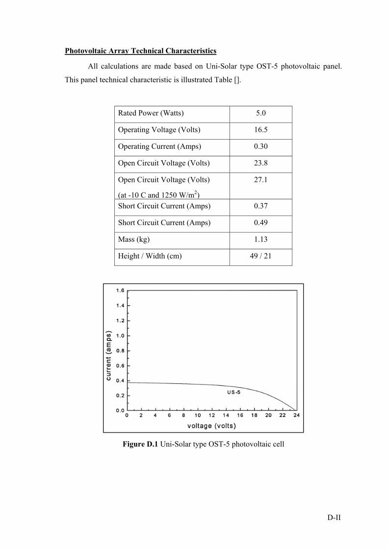
Photovoltaic Array Technical Characteristics
All calculations are made based on Uni-Solar type OST-5 photovoltaic panel.
This panel technical characteristic is illustrated Table [].
Rated Power (Watts) 5.0
Operating Voltage (Volts) 16.5
Operating Current (Amps) 0.30
Open Circuit Voltage (Volts) 23.8
Open Circuit Voltage (Volts)
(at -10 C and 1250 W/m2)
27.1
Short Circuit Current (Amps) 0.37
Short Circuit Current (Amps) 0.49
Mass (kg) 1.13
Height / Width (cm) 49 / 21
Figure D.1 Uni-Solar type OST-5 photovoltaic cell
D-II

APPENDIX E
TWO AXIS SUN TRACKING SOFTWARE VISUAL BASIC CODE
Option Explicit Dim Hgt, Wth As Single Private Sub TileHorizon_Click() SunTracking.Arrange 1 End Sub Private Sub TileVertical_Click() SunTracking.Arrange 2 End Sub Private Sub ArrangeIcons_Click() SunTracking.Arrange 3 End Sub Private Sub Cascade_Click() SunTracking.Arrange 0 End Sub Private Sub About_Click() frmAbout.Show vbModal End Sub Private Sub StepperControl_Click() Stepper.Show Stepper.Form_Load Stepper.Timer1.Enabled = True Stepper.Timer1.Interval = 50 End Sub Private Sub SunCalculation_Click() SunPosition.Show End Sub Private Sub MDIForm_Load() Me.Move 0, 0 Wth = Screen.Width \ Screen.TwipsPerPixelX Hgt = Screen.Height \ Screen.TwipsPerPixelY If Wth = 800 And Hgt = 600 Then SunTracking.Height = 10000 SunTracking.Width = 12000 End If If Wth = 1024 And Hgt = 768 Then SunTracking.Height = 12000 SunTracking.Width = 13000
E-I

End If If Wth = 1280 And Hgt = 1024 Then SunTracking.Height = 12555 SunTracking.Width = 13350 End If SunPosition.ClockTime.Text = Time SunPosition.Date1.Text = Date SunPosition.Show SunPosition.Timer2.Enabled = True SunPosition.Timer2.Interval = 500 exc = 3 Stepper.Show End Sub Private Sub Exit_Click() 'exit Unload Stepper Unload SunPosition Unload SunTracking End End Sub Private Sub StartTrack_Click() 'start track If exc = 6 Or exc = 7 Then Stepper.Ref End If End Sub Private Sub StopTrack_Click() 'stop track Stepper.Timer2.Enabled = False Stepper.Timer3.Enabled = False Stepper.Timer6.Enabled = False DlPortWritePortUshort 888, 0 End Sub 'xxxxxxxxxxxxxxxxxxxxxxxxxxxxxxxxxxxxxxxxxxxxxxxxxxxxxxxxxxxxxxxxxxxxx 'SUN POSITION CALCULATION ' Created by Elvan Armakan 01/Jan/2003 'xxxxxxxxxxxxxxxxxxxxxxxxxxxxxxxxxxxxxxxxxxxxxxxxxxxxxxxxxxxxxxxxxxxxx Option Explicit Dim LatDeg, LatMin, LngDeg, LngMin, Timez, Lstm, Ds, InputMinutesAfterMidnight As Integer Dim Lat, Lat1, Lng, Lng1, LngAdj As Single Dim LatText, LngText As String
E-II

Dim H1, M1, Sec, H As Integer Dim Total, SolarMin As Single Dim Jd As Single Dim Autoflag As Boolean Dim Y, M, D, K, Doy As Integer Dim InDate As String Const Pi As Double = 3.14159265358979 Dim TheHours, TheMinutes As Integer Dim Dtr, Rtd As Single Dim N, T, G, G1, Lambda, L, L1, Alfa, Epsilon, DecAngle, Eot, LsotAdj As Single Dim HourAngle1, Alpha, AzimuthAngle, SunRiseSet, SunRise1, SunSet1 As Single Dim Elev As Integer Dim Flag As Single Dim AppExcel As Excel.Application Dim wSheet As Worksheet Dim wBook As Workbook 'xxxxxxxxxxxxxxxxxxxxxxxxxxxxxxxxxxxxxxxxxxxxxxxxxxxxxx 'SYSTEM TIMEZONE AND DAYLIGHT SAVING 'xxxxxxxxxxxxxxxxxxxxxxxxxxxxxxxxxxxxxxxxxxxxxxxxxxxxxx Private Const TIME_ZONE_ID_DAYLIGHT As Long = 2 Private Type SYSTEMTIME wYear As Integer wMonth As Integer wDayOfWeek As Integer wDay As Integer wHour As Integer wMinute As Integer wSecond As Integer wMilliseconds As Integer End Type Private Type TIME_ZONE_INFORMATION Bias As Long StandardName(0 To 63) As Byte 'unicode (0-based) StandardDate As SYSTEMTIME StandardBias As Long DaylightName(0 To 63) As Byte 'unicode (0-based) DaylightDate As SYSTEMTIME DaylightBias As Long End Type Private Declare Function GetTimeZoneInformation Lib "kernel32" _ (lpTimeZoneInformation As TIME_ZONE_INFORMATION) As Long
E-III
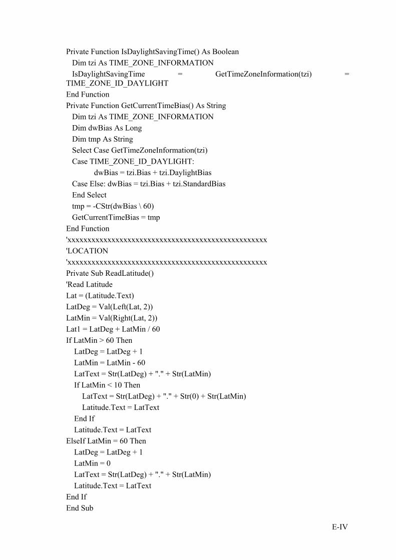
Private Function IsDaylightSavingTime() As Boolean Dim tzi As TIME_ZONE_INFORMATION IsDaylightSavingTime = GetTimeZoneInformation(tzi) = TIME_ZONE_ID_DAYLIGHT End Function Private Function GetCurrentTimeBias() As String Dim tzi As TIME_ZONE_INFORMATION Dim dwBias As Long Dim tmp As String Select Case GetTimeZoneInformation(tzi) Case TIME_ZONE_ID_DAYLIGHT: dwBias = tzi.Bias + tzi.DaylightBias Case Else: dwBias = tzi.Bias + tzi.StandardBias End Select tmp = -CStr(dwBias \ 60) GetCurrentTimeBias = tmp End Function 'xxxxxxxxxxxxxxxxxxxxxxxxxxxxxxxxxxxxxxxxxxxxxxxxxx 'LOCATION 'xxxxxxxxxxxxxxxxxxxxxxxxxxxxxxxxxxxxxxxxxxxxxxxxxx Private Sub ReadLatitude() 'Read Latitude Lat = (Latitude.Text) LatDeg = Val(Left(Lat, 2)) LatMin = Val(Right(Lat, 2)) Lat1 = LatDeg + LatMin / 60 If LatMin > 60 Then LatDeg = LatDeg + 1 LatMin = LatMin - 60 LatText = Str(LatDeg) + "." + Str(LatMin) If LatMin < 10 Then LatText = Str(LatDeg) + "." + Str(0) + Str(LatMin) Latitude.Text = LatText End If Latitude.Text = LatText ElseIf LatMin = 60 Then LatDeg = LatDeg + 1 LatMin = 0 LatText = Str(LatDeg) + "." + Str(LatMin) Latitude.Text = LatText End If End Sub
E-IV

Private Sub ReadLongitude() 'Read Longitude Lng = (Longitude.Text) LngDeg = Val(Left(Lng, 2)) LngMin = Val(Right(Lng, 2)) Lng1 = LngDeg + LngMin / 60 'Longitude Adjustment LngAdj = 4 * (Lng1 - Lstm) If LngMin > 60 Then LngDeg = LngDeg + 1 LngMin = LngMin - 60 LngText = Str(LngDeg) + "." + Str(LngMin) If LngMin < 10 Then LngText = Str(LngDeg) + "." + Str(0) + Str(LngMin) Longitude.Text = LngText End If Longitude.Text = LngText ElseIf LngMin = 60 Then LngDeg = LngDeg + 1 LngMin = 0 LngText = Str(LngDeg) + "." + Str(LngMin) Longitude.Text = LngText End If End Sub Private Sub TimeZone1() 'Time Zone and Local standart Time Timez = Val(TimeZone.Text) Lstm = Timez * 15 TimeZone.Text = Timez End Sub Private Sub TimeZone_Change() Timez = Val(TimeZone.Text) End Sub Private Sub DaylightSaving() 'Day Light Saving Adjustment If DayLight.Text = "Yes" Then Ds = -60 Else Ds = 0 End If End Sub
E-V

Private Sub Ew_Change() 'Longitude East-West Adjustment If Ew.Text = "W" Then Lng1 = -1 * Lng1 Else Lng1 = Lng1 End If End Sub Private Sub Ns_Change() 'Latitude North-South Adjustment If Ns.Text = "S" Then Lat1 = -1 * Lat1 Else Lat1 = Lat1 End If End Sub Private Sub Stop1_Click() Timer1.Enabled = False Timer2.Enabled = False End Sub 'xxxxxxxxxxxxxxxxxxxxxxxxxxxxxxxxxxxxxxxxxxxxxxxxxxxxxx 'AUTOMATIC CALCULATION 'xxxxxxxxxxxxxxxxxxxxxxxxxxxxxxxxxxxxxxxxxxxxxxxxxxxxxx Private Sub Timer1_Timer() 'Import System Timer ClockTime.Text = Time() 'Calculation Hour and Minute for Automatic H1 = Hour(Time) M1 = Minute(Time) Sec = Second(Time) Total = 3600 * H1 + 60 * M1 + Sec 'Calculate clock minutes after midnight InputMinutesAfterMidnight = 60 * H1 + M1 'Solar Minutes After Midnight SolarMin = InputMinutesAfterMidnight + LngAdj + Ds 'Automatic Sun calculation for 2,4,8,10,16 Minutes If Total Mod (Interval.Text * 60) = 0 And Autoflag = True Then Autocal_Click End If End Sub Private Sub Timer2_Timer()
E-VI

Flag = Flag + 1 If exc = 3 And Flag = 2 Then First End If If exc = 4 And Flag = 4 Then Second1 End If If exc = 5 And Flag = 6 Then Third End If End Sub Public Sub First() Set AppExcel = CreateObject("Excel.Application") Set wBook = AppExcel.Workbooks.Add 'First time 'Import System Timer ClockTime.Text = Time() H1 = Hour(Time) M1 = Minute(Time) Sec = Second(Time) Total = 3600 * H1 + 60 * M1 + Sec InputMinutesAfterMidnight = 60 * H1 + M1 SolarMin = InputMinutesAfterMidnight + LngAdj + Ds Autocal_Click Timer1.Enabled = False End Sub Public Sub Second1() 'to calculate using sunrisetime H1 = Left(SunRise.Text, 2) M1 = Right(SunRise.Text, 2) Sec = 0 Total = 3600 * H1 + 60 * M1 + Sec InputMinutesAfterMidnight = 60 * H1 + M1 SolarMin = InputMinutesAfterMidnight + LngAdj + Ds Autocal_Click End Sub Public Sub Third() 'to calculate using system time ClockTime.Text = Time() H1 = Hour(Time) M1 = Minute(Time)
E-VII

Sec = Second(Time) Total = 3600 * H1 + 60 * M1 + Sec InputMinutesAfterMidnight = 60 * H1 + M1 SolarMin = InputMinutesAfterMidnight + LngAdj + Ds Autocal_Click Timer1.Enabled = True Timer2.Enabled = False Timer2.Interval = 0 Main Stepper.Show End Sub Public Sub Autocal_Click() Autoflag = True 'Read Value ReadLatitude ReadLongitude TimeZone1 DaylightSaving 'Import System Date Date = Date1.Text Y = Year(Date) M = Month(Date) D = Day(Date) 'Day of Year If Y Mod 4 = 0 Then K = 1 Else K = 2 End If Doy = Int((275 * M) / 9) - K * Int((M + 9) / 12) + D - 30 DayofYear.Text = Doy 'Sun Path Calculation exc = exc + 1 Astronomic End Sub Public Sub Form_Load() 'Day light Saving DayLight.AddItem "Yes" DayLight.AddItem "No" If IsDaylightSavingTime() = False Then DayLight.Text = "No"
E-VIII

Else DayLight.Text = "Yes" End If 'North-South Adjustment Ns.AddItem "N" Ns.AddItem "S" 'East-West Adjustment Ew.AddItem "E" Ew.AddItem "W" 'Time Zone TimeZone.Text = GetCurrentTimeBias() TimeZone.AddItem "UT" TimeZone.AddItem " +1" TimeZone.AddItem " +2" TimeZone.AddItem " +3" TimeZone.AddItem " -1" TimeZone.AddItem " -2" TimeZone.AddItem " -3" 'Time interval Interval.AddItem " 2" Interval.AddItem " 4" Interval.AddItem " 8" 'System Date and Time Date1.Text = Date ClockTime.Text = Time() 'Default Value Latitude.Text = "38.25" Longitude.Text = "27.15" Elev1.Text = "0" Ns.Text = "N" Ew.Text = "E" Interval.Text = " 2" End Sub 'xxxxxxxxxxxxxxxxxxxxxxxxxxxxxxxxxxxxxxxxxxxxxxxxxxxxxxxxxxxxx 'MANUAL CALCULATION SOFTWARE 'xxxxxxxxxxxxxxxxxxxxxxxxxxxxxxxxxxxxxxxxxxxxxxxxxxxxxxxxxxxxx Private Sub Manualcal_Click() 'Longitude East-West Adjustment If Ew.Text = "W" Then Lng1 = -1 * Lng1 Else
E-IX

Lng1 = Lng1 End If 'Latitude North-South Adjustment If Ns.Text = "S" Then Lat1 = -1 * Lat1 Else Lat1 = Lat1 End If Autoflag = False Timer1.Enabled = False Timer1.Interval = 0 'Clear TextBox Declination.Text = "" Equation.Text = "" LocalSolarTime.Text = "" HourAngle.Text = "" Altitude.Text = "" Azimuth.Text = "" SunSet.Text = "" SunRise.Text = "" DayofYear.Text = "" DayLength.Text = "" 'Read Value ReadLatitude ReadLongitude TimeZone1 DaylightSaving If Hour1.Text = "" Then MsgBox ("Input Hour : Minute") End If If InputDate.Text = "" Then MsgBox ("Select Date") End If If Hour1.Text <> "" And H1 <= 24 And InputDate.Text <> "" Then 'Sun path Calculation ManualHM Astronomic End If End Sub Private Sub ManualHM() H1 = Left(Hour1.Text, 2)
E-X

M1 = Right(Hour1.Text, 2) If M1 > 60 And H1 < 24 Then M1 = M1 - 60 H1 = H1 + 1 Hour1.Text = Str(H1) + ":" + Str(M1) End If If M1 > 60 And H1 = 24 Then M1 = M1 - 60 H1 = 1 Hour1.Text = Str(0) + Str(H1) + ":" + Str(M1) End If If H1 > 24 Then MsgBox ("Day includes only 24 hours") End If Total = 3600 * H1 + 60 * M1 'Calculate clock minutes after midnight InputMinutesAfterMidnight = 60 * H1 + M1 'Solar Minutes After Midnight SolarMin = InputMinutesAfterMidnight + LngAdj + Ds 'Input Day, Month, Year If InputDate.Text <> "" Then D = Left(InDate, 2) M1 = Left(InDate, 5) M = Right(M1, 2) Y = Right(InDate, 4) If Y < 1998 Or Y > 2021 Then MsgBox ("This Year is out of calculation; Enter new date!") End If 'Day of Year If Y Mod 4 = 0 Then K = 1 Else K = 2 End If Doy = Int((275 * M) / 9) - K * Int((M + 9) / 12) + D - 30 DayofYear.Text = Doy End If End Sub Private Sub MonthView1_DateClick(ByVal DateClicked As Date) 'Close date InputDate.Text = MonthView1.Value
E-XI

InDate = InputDate.Text End Sub 'xxxxxxxxxxxxxxxxxxxxxxxxxxxxxxxxxxxxxxxxxxxxxxxxxxxxxxxxxxxx 'ASTRONOMICAL SUN POSITION FORMULATION 'xxxxxxxxxxxxxxxxxxxxxxxxxxxxxxxxxxxxxxxxxxxxxxxxxxxxxxxxxxxx Private Sub Astronomic() Select Case Y Case 1998 Jd = -731.5 Case 1999 Jd = -366.5 Case 2000 Jd = -1.5 Case 2001 Jd = 364.5 Case 2002 Jd = 729.5 Case 2003 Jd = 1094.5 Case 2004 Jd = 1459.5 Case 2005 Jd = 1825.5 Case 2006 Jd = 2190.5 Case 2007 Jd = 2555.5 Case 2008 Jd = 2920.5 Case 2009 Jd = 3286.5 Case 2010 Jd = 3651.5 Case 2011 Jd = 4016.5 Case 2012 Jd = 4381.5 Case 2013 Jd = 4747.5 Case 2014 Jd = 5112.5
E-XII

Case 2015 Jd = 5477.5 Case 2016 Jd = 5842.5 Case 2017 Jd = 6208.5 Case 2018 Jd = 6573.5 Case 2019 Jd = 6938.5 Case 2020 Jd = 7303.5 Case 2021 Jd = 7669.5 End Select 'Constant Dtr = Pi / 180 Rtd = 180 / Pi 'SUN CALCULATION N = Jd + Doy + ((SolarMin / 60) / 24) 'Mean Longitude of Sun ,corrected for aberration L1 = 280.46 + 0.9856474 * N L = NormalizeTo360(L1) 'Mean Anormaly G1 = 357.528 + 0.9856003 * N G = NormalizeTo360(G1) 'Ecliptic Longitude Lambda = L + (1.915 * Sin(G * Dtr)) + (0.02 * Sin(2 * G * Dtr)) 'Obliquity of ecliptic Epsilon = 23.439 - 0.0000004 * N 'Right ascension T = (Tan(Dtr * Epsilon / 2)) ^ 2 Alfa = Lambda - Rtd * T * Sin(2 * Lambda * Dtr) + 0.5 * Rtd * (T ^ 2) * Sin(4 * Lambda * Dtr) 'declination DecAngle = ArcSin(Sin(Epsilon * Dtr) * Sin(Lambda * Dtr)) Declination.Text = Round(DecAngle, 2) 'Equation of Time Eot = (L - Alfa) * 4 Equation.Text = Round(Eot, 2) 'Calculate the difference between solar time and clock time computed the equation of time
E-XIII

LsotAdj = 4 * (Lng1 - Lstm) + Round(Eot, 2) + Ds LngAdj = LsotAdj 'New Solar Time SolarMin = InputMinutesAfterMidnight + LsotAdj LocalSolarTime.Text = MinuteToHour(SolarMin) 'Hour Angle HourAngle1 = ((SolarMin - 12 * 60) / 4) HourAngle.Text = Round(HourAngle1, 2) 'Altitude Angle Alpha = ArcSin(Cos(Dtr * Lat1) * Cos(DecAngle * Dtr) * Cos(HourAngle1 * Dtr) + Sin(Lat1 * Dtr) * Sin(DecAngle * Dtr)) If Sgn(Alpha) = -1 Then Altitude.Text = "0" Else Altitude.Text = Round(Alpha, 2) End If 'Azimuth Angle If HourAngle1 = 0 Then AzimuthAngle = 0 End If AzimuthAngle = Arccos((Sin(Alpha * Dtr) * Sin(Lat1 * Dtr) - Sin(DecAngle * Dtr)) / (Cos(Alpha * Dtr) * Cos(Lat1 * Dtr))) If (AzimuthAngle * HourAngle1) < 0 Then AzimuthAngle = -1 * AzimuthAngle End If Azimuth.Text = Round(AzimuthAngle, 2) 'Clock Time of Sunrise & Sunset Elev = Int(Fix(Elev1.Text)) SunRiseSet = Arccos(-1 * Sin(Lat1 * Dtr) * Sin(DecAngle * Dtr) - Sin((-0.8333 - 0.0347 * Sqr(Elev)) * Dtr) / (Cos(Lat1 * Dtr) * Cos(DecAngle * Dtr))) * 4 SunRise1 = ((12 * 60 - SunRiseSet - (4 * (Lng1 - Lstm)) - Eot - Ds)) SunRise.Text = MinuteToHour(SunRise1) SunSet1 = ((12 * 60 + SunRiseSet - (4 * (Lng1 - Lstm)) - Eot - Ds)) SunSet.Text = MinuteToHour(SunSet1) If (Total / 60) > SunSet1 Or (Total / 60) < SunRise1 Then Azimuth.Text = "0" End If If exc = 5 Then Alt1(0) = Altitude.Text Azm1(0) = Azimuth.Text End If 'Day Lenght
E-XIV

DayLength.Text = MinuteToHour(2 * SunRiseSet) If exc = 6 Then Alt1(1) = Altitude.Text Azm1(1) = Azimuth.Text End If Alt = Alt1(1) - Alt1(0) Azm = Azm1(1) - Azm1(0) If Autocal2.Caption = "Automatic Calculation" Then FormExcel End If End Sub 'xxxxxxxxxxxxxxxxxxxxxxxxxxxxxxxxxxxxxxxxxxxxxxxxxxxxxxxxxxxxxxxxxxxx 'FUNCTION 'xxxxxxxxxxxxxxxxxxxxxxxxxxxxxxxxxxxxxxxxxxxxxxxxxxxxxxxxxxxxxxxxxxxx Public Function ArcSin(Sine) 'Arc Sinus Function If Abs(Sine) < 0.99999999 Then ArcSin = (180 / Pi) * Atn(Sine / Sqr(-Sine * Sine + 1)) Else ArcSin = 90 * Sgn(Sine) End If End Function Public Function Arccos(Cosine) 'Arc Cosinus Function If Abs(Cosine) < 0.99999999 Then Arccos = 90 - (180 / Pi) * Atn(Cosine / Sqr(-Cosine * Cosine + 1)) Else Arccos = 90 - 90 * Sgn(Cosine) End If End Function Public Function NormalizeTo360(Thing) 'Normalize Angle NormalizeTo360 = Thing - Int(Thing / 360) * 360 End Function Public Function MinuteToHour(TotalMinutes) 'Turn Total Minutes to Hour and Minutes TheHours = Fix(TotalMinutes / 60) TheMinutes = Int(TotalMinutes - Fix(TotalMinutes / 60) * 60) MinuteToHour = (Str(TheHours) + ":" + Str(TheMinutes)) End Function
E-XV

'xxxxxxxxxxxxxxxxxxxxxxxxxxxxxxxxxxxxxxxxxxxxxxxxxxxxxxxxxxxxxxxxxx 'EXCEL APPLICATION 'xxxxxxxxxxxxxxxxxxxxxxxxxxxxxxxxxxxxxxxxxxxxxxxxxxxxxxxxxxxxxxxxxx Public Sub FormExcel() Set wSheet = AppExcel.Sheets(1) wSheet.Cells(2, 1).Value = " DATE " wSheet.Cells(2, 2).Value = "DAY-YEAR" wSheet.Cells(2, 3).Value = " HOUR " wSheet.Cells(2, 4).Value = "HOUR ANGLE" wSheet.Cells(2, 5).Value = "EQ OFTIME" wSheet.Cells(2, 6).Value = "DECLINATION" wSheet.Cells(2, 7).Value = "ALTITUDE" wSheet.Cells(2, 8).Value = "AZIMUTH" wSheet.Cells(2, 9).Value = "SUN RISE" wSheet.Cells(2, 10).Value = "SUN SET" wSheet.Cells(2, 11).Value = "DAY LENGTH" wSheet.Cells(2, 12).Value = "STEPPER-1" wSheet.Cells(2, 13).Value = "STEPPER-2" wSheet.Cells(2, 14).Value = "RUNNING-1" wSheet.Cells(2, 15).Value = "RUNNING-2" wSheet.Cells(2, 16).Value = "TOTAL-1" wSheet.Cells(2, 17).Value = "TOTAL-2" wSheet.Cells(2, 18).Value = "RUNNING-1 STEPS" wSheet.Cells(2, 19).Value = "RUNNING-2 STEPS" wSheet.Cells(2, 20).Value = "TOTAL-1 STEPS" wSheet.Cells(2, 21).Value = "TOTAL-2 STEPS" wSheet.Cells(exc, 1).Value = SunPosition.Date1.Text wSheet.Cells(exc, 2).Value = SunPosition.DayofYear.Text wSheet.Cells(exc, 3).Value = SunPosition.ClockTime.Text wSheet.Cells(exc, 4).Value = SunPosition.HourAngle.Text wSheet.Cells(exc, 5).Value = SunPosition.Equation.Text wSheet.Cells(exc, 6).Value = SunPosition.Declination.Text wSheet.Cells(exc, 7).Value = SunPosition.Altitude.Text wSheet.Cells(exc, 8).Value = SunPosition.Azimuth.Text wSheet.Cells(exc, 9).Value = SunPosition.SunRise.Text wSheet.Cells(exc, 10).Value = SunPosition.SunSet.Text wSheet.Cells(exc, 11).Value = SunPosition.DayLength.Text wSheet.Cells(exc, 12).Value = Stepper.NorthSouth.Text wSheet.Cells(exc, 13).Value = Stepper.EastWest.Text wSheet.Cells(exc, 14).Value = Stepper.Text1.Text
E-XVI

wSheet.Cells(exc, 15).Value = Stepper.Text2.Text wSheet.Cells(exc, 16).Value = Stepper.Text3.Text wSheet.Cells(exc, 17).Value = Stepper.Text4.Text wSheet.Cells(exc, 18).Value = Stepper.Text5.Text wSheet.Cells(exc, 19).Value = Stepper.Text6.Text wSheet.Cells(exc, 20).Value = Stepper.Text7.Text wSheet.Cells(exc, 21).Value = Stepper.Text8.Text Range("A2:M2").Select With Selection.Font .Name = "Verdana" .FontStyle = "Bold" .Size = 10 End With Range("A2:M2").Select Selection.Columns.AutoFit Range("A2:M2").Select With Selection .HorizontalAlignment = xlCenter End With Range("A3: M3").Select With Selection .HorizontalAlignment = xlCenter End With AppExcel.Visible = True End Sub 'xxxxxxxxxxxxxxxxxxxxxxxxxxxxxxxxxxxxxxxxxxxxxxxxxxxxxxxxxxxxxxxx 'STEPPER MOTOR CONTROL PROGRAM 'Created By 'xxxxxxxxxxxxxxxxxxxxxxxxxxxxxxxxxxxxxxxxxxxxxxxxxxxxxxxxxxxxxxxx Option Explicit Dim Delay1, Delay2, Step1, Step2 As Integer Dim D1 As Boolean Dim D2 As Boolean Dim Min, Now, Now1, StepInMillisecs As Long Dim R, R1, F1, F2 As Integer Dim St1, K1, K2 As Integer Dim X, Y, Nsd, Ewd, i, j As Integer Dim Br1 As Boolean Dim Br2 As Boolean Dim Ralt As Boolean
E-XVII

Dim Razm As Boolean Dim O1, O2 As Boolean Dim Altin As Boolean Dim Altref As Boolean Dim Altauto As Single Dim Sens As Single Dim LF1 As Boolean Dim LF2 As Boolean Dim Azmin As Boolean Dim Azmref As Boolean Dim Azmauto As Single Dim AutoAzm As Boolean Dim AutoAlt As Boolean Dim Cloudy, C As Boolean Dim Autoflag As Boolean Dim Start1Time As Single Dim Stop1Time As Single Dim Net1Time As Single Dim Start2Time As Single Dim Stop2Time As Single Dim Net2Time As Single Dim Net1Time1 As Single Dim Net2Time2 As Single Dim TotalStep2 As Single Dim TotalStep1 As Single 'xxxxxxxxxxxxxxxxxxxxxxxxxxxxxxxxxxxxxxxxxxxxxxxxxxxxxxxxxxxxxxxxxxxxxxxxxxxxxxxxxxxxxxxxxxxxxxxxx 'INPUT SIGNAL PROGRAM 'xxxxxxxxxxxxxxxxxxxxxxxxxxxxxxxxxxxxxxxxxxxxxxxxxxxxxxxxxxxxxxxxxxxxxxxxxxxxxxxxxxxxxxxxxxxxxxxxx Private Sub Timer1_Timer() R1 = DlPortReadPortUchar(889) If R1 <> R Then Status1 End If Altitude1.Text = SunPosition.Altitude.Text Azimuth1.Text = SunPosition.Azimuth.Text End Sub Private Sub Status1() 'Read paralel port R = DlPortReadPortUchar(889) Select Case R
E-XVIII

Case 127 Or 126 Input1.Text = "No Signal" Ralt = False Razm = False LF1 = False LF2 = False Cloudy = False Case 111 Or 110 Input1.Text = "Signal S1" Ralt = True Razm = False LF1 = False LF2 = False Cloudy = False Case 255 Or 254 Input1.Text = "Signal S2" Ralt = False Razm = True LF1 = False LF2 = False Cloudy = False Case 95 Or 94 Input1.Text = "Signal F1" Ralt = False Razm = False LF1 = True LF2 = False Cloudy = False Case 63 Or 62 Input1.Text = "Signal F2" Ralt = False Razm = False LF1 = False LF2 = True Cloudy = False Case 119 Or 118 Input1.Text = "Signal Cloudiness" Ralt = False Razm = False LF1 = False LF2 = False
E-XIX
Cloudy = True Case 247 Or 246 Input1.Text = "Signal S2-C" Ralt = False Razm = True LF1 = False LF2 = False Cloudy = True Case 103 Or 102 Input1.Text = "Signal S1-C" Ralt = True Razm = False LF1 = False LF2 = False Cloudy = True Case 87 Or 86 Input1.Text = "Signal F1-C" Ralt = False Razm = False LF1 = True LF2 = False Cloudy = True Case 55 Or 54 Input1.Text = "Signal F2-C" Ralt = False Razm = False LF1 = False LF2 = True Cloudy = True Case 231 Or 230 Input1.Text = "Signal S1-S2-C" Ralt = True Razm = True LF1 = False LF2 = False Cloudy = True Case 183 Or 182 Input1.Text = "Signal S2-F2-C" Ralt = False Razm = True LF1 = False
E-XX
LF2 = True Cloudy = True Case 215 Or 214 Input1.Text = "Signal S2-F1-C" Ralt = False Razm = True LF1 = True LF2 = False Cloudy = True Case 71 Or 70 Input1.Text = "Signal S1-F1-C" Ralt = True Razm = False LF1 = True LF2 = False Cloudy = True Case 39 Or 38 Input1.Text = "Signal S1-F2-C" Ralt = True Razm = False LF1 = False LF2 = True Cloudy = True Case 239 Or 238 Input1.Text = "Signal S1-S2" Ralt = True Razm = True LF1 = False LF2 = False Cloudy = False Case 79 Or 78 Input1.Text = "Signal S1-F1" Ralt = True Razm = False LF1 = True LF2 = False Cloudy = False Case 47 Or 46 Input1.Text = "Signal S1-F2" Ralt = True Razm = False
E-XXI

LF1 = False LF2 = True Cloudy = False Case 223 Or 222 Input1.Text = "Signal S2-F1" Ralt = False Razm = True LF1 = True LF2 = False Cloudy = False Case 191 Or 190 Input1.Text = "Signal S2-F2" Ralt = False Razm = True LF1 = False LF2 = True Cloudy = False Case 31 Or 30 Input1.Text = "Signal F1-F2" Ralt = False Razm = False LF1 = True LF2 = True Cloudy = False Case 207 Or 206 Input1.Text = "Signal S1-S2-F1" Ralt = True Razm = True LF1 = True LF2 = False Cloudy = False Case 175 Or 174 Input1.Text = "Signal S1-S2-F2" Ralt = True Razm = True LF1 = False LF2 = True Cloudy = False Case 15 Or 14 Input1.Text = "Signal S1-F1-F2" Ralt = True
E-XXII
Razm = False LF1 = True LF2 = True Cloudy = False Case 159 Or 158 Input1.Text = "Signal S2-F1-F2" Ralt = False Razm = True LF1 = True LF2 = True Cloudy = False Case 143 Or 142 Input1.Text = "Signal S1-S2-F1-F2" Ralt = True Razm = True LF1 = True LF2 = True Cloudy = False End Select End Sub 'xxxxxxxxxxxxxxxxxxxxxxxxxxxxxxxxxxxxxxxxxxxxxxxxx 'START AUTOMATIC SUN TRACKING 'xxxxxxxxxxxxxxxxxxxxxxxxxxxxxxxxxxxxxxxxxxxxxxxxx Private Sub Command4_Click() If exc = 6 Or exc = 7 Then Ref End If C = True End Sub 'REFERENCE POINT CONTROL Public Sub Ref() If Razm = False Then Ref2 Azmref = True End If 'if panel does not stay referance point If Razm = True And Ralt = False Then Ref1 Altref = True Timer4.Enabled = False Timer4.Interval = 0
E-XXIII
End If If Razm = True And Ralt = True Then Initial Azmref = True Altref = True Timer4.Enabled = False Timer4.Interval = 0 End If End Sub Private Sub Referance1_Click(Index As Integer) Ref1 Altref = False End Sub Public Sub Ref1() If Ralt = False Then 'if panel does not stay referance point-1 O1 = False D1 = False X = 0 Step1 = 1440 Start1Time = GetTickCount Timer2.Enabled = True Timer2.Interval = 50 End If If Ralt = True Then Timer2.Enabled = False Timer2.Interval = 0 End If End Sub Private Sub Referance2_Click(Index As Integer) Ref2 Azmref = False End Sub Private Sub Ref2() If Razm = False And LF1 = False And LF2 = False Then 'if panel does not stay referance point-2 O2 = False D2 = False Y = 0 Step2 = 1500 Start2Time = GetTickCount Timer3.Enabled = True Timer3.Interval = 50
E-XXIV

End If If Razm = False And LF1 = True Then O2 = False D2 = False Y = 0 Start2Time = GetTickCount Step2 = 1500 Timer3.Enabled = True Timer3.Interval = 50 End If If Razm = False And LF2 = True Then O2 = False D2 = True Y = 0 Start2Time = GetTickCount Step2 = 1500 Timer3.Enabled = True Timer3.Interval = 50 End If If Razm = True Then Timer3.Enabled = False Timer3.Interval = 0 End If End Sub Private Sub Timer4_Timer() 'Automatic tracking If Razm = True Then WaitTime 1000 Ref End If End Sub 'INITIAL AZIMUTH AND ALTITUDE Private Sub Initial() 'Initially azimuth If Cloudy = False Then If Motor2.Value = 1 Then If SunPosition.Azimuth.Text <= "1.8" And SunPosition.Azimuth.Text <= "-1.8" Then EastWest.Text = "0" Timer5.Enabled = True Timer5.Interval = 3000 End If
E-XXV
If SunPosition.Azimuth.Text > "1.8" Or SunPosition.Azimuth.Text > "-1.8" Then O2 = True Step2 = Round(4 * Abs(Azm) / 0.9) If Sgn(Azm) = -1 Then D2 = True EastWest.Text = Format((-1 * Step2 * 0.9 / 4), "##.##") ElseIf Sgn(Azm) = 1 Then D2 = False EastWest.Text = Format((Step2 * 0.9 / 4), "##.##") End If X = 0 Azmin = True Start2Time = GetTickCount Timer3.Enabled = True Timer3.Interval = Delay2 End If If SunPosition.Azimuth.Text = "0" And Razm = True Then EastWest.Text = "0" Timer5.Enabled = True Timer5.Interval = 3000 End If Else EastWest.Text = "0" Timer5.Enabled = True Timer5.Interval = 3000 Azmin = False End If End If End Sub Private Sub Timer5_Timer() Inalt End Sub Private Sub Inalt() 'Initially Altitude If Cloudy = False Then If Motor1.Value = 1 Then If SunPosition.Altitude.Text <> "0" Then 'Altitude angle is not equal to zero O1 = True Step1 = Round(4 * Abs(Alt) / 0.9)
E-XXVI

D1 = True X = 0 NorthSouth.Text = Format((Step1 * 0.9 / 4), "##.##") Altin = True Start1Time = GetTickCount Timer2.Enabled = True Timer2.Interval = Delay1 Timer5.Enabled = False Timer5.Interval = 0 End If If SunPosition.Altitude.Text = "0" Then 'Altitude angle is equal to zero NorthSouth.Text = "0" Timer5.Enabled = False Timer5.Interval = 0 Timer6.Enabled = True Timer6.Interval = 10000 End If Else Altin = False Timer5.Enabled = True Timer5.Interval = 0 Timer6.Enabled = True Timer6.Interval = 60000 D1 = True O1 = True Start1Time = GetTickCount Step1 = 132 Timer2.Enabled = True Timer2.Interval = Delay1 End If End If End Sub 'AUTOMATIC TRACKING Private Sub Timer6_Timer() Altin = False Azmin = False 'Automatic tracking Altauto = Val((SunPosition.Altitude.Text) - (NorthSouth.Text)) Azmauto = Val((SunPosition.Azimuth.Text) - (EastWest.Text)) If exc > 7 And Abs(Azmauto) >= Sens And Motor2.Value = 1 And Cloudy = False Then AutoAzimuth
E-XXVII
Autoflag = True End If If exc > 7 And Abs(Altauto) >= Sens And Motor1.Value = 1 And Autoflag = False And Cloudy = False Then AutoAltitude End If End Sub Public Sub AutoAzimuth() 'automatic stepper motor control If Sgn(Azmauto) = 1 Then AutoAzm = True D2 = False Y = 0 Step2 = Round(Abs(Azmauto) * 4 / 0.9) EastWest.Text = SunPosition.Azimuth.Text Start2Time = GetTickCount Timer3.Enabled = True Timer3.Interval = Delay2 Timer6.Enabled = False Timer6.Interval = 0 ElseIf Sgn(Azmauto) = -1 Then AutoAzm = True D2 = True Y = 0 Step2 = Round(Abs(Azmauto) * 4 / 0.9) EastWest.Text = SunPosition.Azimuth.Text Start2Time = GetTickCount Timer3.Enabled = True Timer3.Interval = Delay2 Timer6.Enabled = False Timer6.Interval = 0 End If If Azmauto = 0 Then Ref2 Timer6.Enabled = False Timer6.Interval = 0 End If End Sub Public Sub AutoAltitude() If Sgn(Altauto) = 1 Then AutoAlt = True D1 = True
E-XXVIII

X = 0 Step1 = Round(Abs(Altauto) * 4 / 0.9) Start1Time = GetTickCount NorthSouth.Text = SunPosition.Altitude.Text Timer2.Enabled = True Timer2.Interval = Delay1 Timer6.Enabled = False Timer6.Interval = 0 End If If Sgn(Altauto) = -1 Then AutoAlt = True D1 = False X = 0 Step1 = Round(Abs(Altauto) * 4 / 0.9) Start1Time = GetTickCount NorthSouth.Text = SunPosition.Altitude.Text Timer2.Enabled = True Timer2.Interval = Delay1 Timer6.Enabled = False Timer6.Interval = 0 End If If Altauto = 0 Then Ref1 Timer6.Enabled = False Timer6.Interval = 0 End If End Sub Private Sub Motor1_Click() 'working only stepper-1 If Motor1.Value = 1 Then Autoflag = False Else Autoflag = True End If End Sub Private Sub Motor2_Click() 'working only stepper -2 If Motor2.Value = 1 Then Autoflag = True Else Autoflag = False
E-XXIX

End If End Sub Private Sub Timer7_Timer() 'Cloudiness ON/OFF If Cloudy = False And C = True And exc > 7 And Timer6.Enabled = False Then Timer6.Enabled = True Timer6.Interval = 10000 End If End Sub 'xxxxxxxxxxxxxxxxxxxxxxxxxxxxxxxxxxxxxxxxxxxxxxxxxxxxxxxxxxxxxxxxxxxxx 'OUTPUT SIGNAL PROGRAM 'xxxxxxxxxxxxxxxxxxxxxxxxxxxxxxxxxxxxxxxxxxxxxxxxxxxxxxxxxxxxxxxxxxxxx Public Sub Form_Load() Azmin = False Altin = False Azmref = False Altref = False AutoAlt = False AutoAzm = False Delay1 = Slider1.Value Delay2 = Slider2.Value Option1.Value = True C = False DlPortWritePortUshort 888, 0 Timer1.Enabled = True Timer1.Interval = 50 Break1.Value = 1 Break2.Value = 1 Combo3.ListIndex = 1 TotalStep1 = 0 TotalStep2 = 0 End Sub 'DELAY TIME Private Sub Slider1_Change() Delay1 = Slider1.Value End Sub Private Sub Slider2_Change() Delay2 = Slider2.Value End Sub Private Sub Option1_Click() 'stepper motor step
E-XXX

Label8(0).Caption = "Steps" Label8(1).Caption = "Steps" End Sub Private Sub Option2_Click() 'stepper motor angle Label8(0).Caption = "Degrees" Label8(1).Caption = "Degrees" End Sub 'xxxxxxxxxxxxxxxxxxxxxxxxxxxxxxxxxxxxxxx 'TRACKING SENSITIVITY 'xxxxxxxxxxxxxxxxxxxxxxxxxxxxxxxxxxxxxxx Private Sub Combo3_Click() If Combo3.ListIndex = 0 Then '8 motor 's steps equal to 1.8 degree panel or disc angle Sens = Val(1.8) End If If Combo3.ListIndex = 1 Then '16 motor 's steps equal to 3.6 degree panel or disc angle Sens = Val(3.6) End If If Combo3.ListIndex = 2 Then '24 motor 's steps equal to 5.4 degree panel or disc angle Sens = Val(5.4) End If If Combo3.ListIndex = 3 Then '32 motor 's steps equal to 7.2 degree panel or disc angle Sens = Val(7.2) End If If Combo3.ListIndex = 4 Then '64 motor 's steps equal to 14.4 degree panel or disc angle Sens = Val(14.4) End If End Sub 'xxxxxxxxxxxxxxxxxxxxxxxxxxxxxxxxxxxxxxx 'DIRECTION 'xxxxxxxxxxxxxxxxxxxxxxxxxxxxxxxxxxxxxxx Private Sub Check1_Click() 'Direction North-South for Step motor-1 (Altitude Angle) If Check1.Value = 0 Then D1 = True 'North Direction Check1.Caption = "Direction (North)"
E-XXXI

Else D1 = False 'South Direction Check1.Caption = "Direction (South)" End If End Sub Private Sub Check2_Click() 'Direction East-West for Step motor-2 (Azimuth Angle) If Check2.Value = 0 Then D2 = True 'East Direction Check2.Caption = "Direction (East)" Else D2 = False 'West Direction Check2.Caption = "Direction (West)" End If End Sub 'xxxxxxxxxxxxxxxxxxxxxxxxxxxxxxxxxxxxxx 'BRAKE SYSTEM 'xxxxxxxxxxxxxxxxxxxxxxxxxxxxxxxxxxxxxx Private Sub Break1_Click() If Break1.Value = 1 Then Br1 = True Else Br1 = False End If Break End Sub Private Sub Break2_Click() If Break2.Value = 1 Then Br2 = True Else Br2 = False End If Break End Sub Private Function Break() If Br1 = True And Br2 = False Then DlPortWritePortUshort 890, 3 End If If Br1 = False And Br2 = True Then DlPortWritePortUshort 890, 15 End If
E-XXXII

If Br1 = False And Br2 = False Then DlPortWritePortUshort 890, 11 End If If Br1 = True And Br2 = True Then DlPortWritePortUshort 890, 7 End If End Function 'xxxxxxxxxxxxxxxxxxxxxxxxxxxxxxxxxxxxxxx 'RUNNING STEPPER MOTOR-1 'xxxxxxxxxxxxxxxxxxxxxxxxxxxxxxxxxxxxxxx Private Sub StepMotor1_Click() If Option1 = True Then Step1 = Round(Abs(Val(Rotation1.Text) * 4)) End If If Option2 = True Then Step1 = Round(Abs(Val(Rotation1.Text) * 4 / 0.86)) End If Timer2.Enabled = True Timer2.Interval = Delay1 X = 0 O1 = True If Check1.Value = 0 Then D1 = True 'North Direction Check1.Caption = "Direction (North)" Else D1 = False 'South Direction Check1.Caption = "Direction (South)" End If If Rotation1.Text = "" Then MsgBox (" Enter Value (Steps or Angle)") End If Start1Time = GetTickCount End Sub Private Sub Timer2_Timer() 'if panel does not stay referance point initially If Ralt = True And O1 = False And Altref = False Then K1 = Step1 ElseIf Ralt = True And O1 = False And Altref = True Then K1 = Step1 Timer4.Enabled = True Timer4.Interval = 100
E-XXXIII

End If If Altin = True And O1 = True And K1 = Step1 - 4 Then Timer6.Enabled = True Timer6.Interval = 10000 End If If AutoAlt = True And K1 = Step1 - 2 Then Timer6.Enabled = True Timer6.Interval = 10000 AutoAlt = False End If 'Brake system If Br1 = True And Br2 = True Then DlPortWritePortUshort 890, 15 ElseIf Br1 = True And Br2 = False Then DlPortWritePortUshort 890, 11 End If 'HALF PHASE DRIVING MODE If D1 = True Then Nsd = 1 Else Nsd = 48 End If If K1 < Step1 Then X = 1 If i Mod 8 = 0 Then DlPortWritePortUshort 888, Fix(Nsd / 48) * X + Fix(9 / Nsd) * X '1 End If If i Mod 8 = 1 Then DlPortWritePortUshort 888, Fix(Nsd / 16) * X + Fix(8 / Nsd) * X '3 End If If i Mod 8 = 2 Then DlPortWritePortUshort 888, Fix(Nsd / 24) * X + Fix(12 / Nsd) * X '2 End If If i Mod 8 = 3 Then DlPortWritePortUshort 888, Fix(Nsd / 8) * X + Fix(4 / Nsd) * X '6 End If If i Mod 8 = 4 Then DlPortWritePortUshort 888, Fix(Nsd / 12) * X + Fix(6 / Nsd) * X '4 End If If i Mod 8 = 5 Then DlPortWritePortUshort 888, Fix(Nsd / 4) * X + Fix(2 / Nsd) * X '12
E-XXXIV

End If If i Mod 8 = 6 Then DlPortWritePortUshort 888, Fix(Nsd / 6) * X + Fix(3 / Nsd) * X '8 End If If i Mod 8 = 7 Then DlPortWritePortUshort 888, Fix(Nsd / 5) * X + Fix(1 / Nsd) * X '9 End If i = i + 1 K1 = K1 + 1 End If 'Stop motor If K1 = Step1 Then If Br1 = True And Br2 = False Then DlPortWritePortUshort 890, 3 ElseIf Br1 = True And Br2 = True Then DlPortWritePortUshort 890, 7 End If K1 = 0 DlPortWritePortUshort 888, 0 Timer2.Interval = 0 Stop1Time = GetTickCount Net1Time1 = (Stop1Time - Start1Time) Stepper.Text1.Text = Net1Time1 Net1Time = (Stop1Time - Start1Time) + Net1Time Stepper.Text3.Text = Net1Time Stepper.Text5.Text = Step1 TotalStep1 = TotalStep1 + Step1 Stepper.Text7.Text = TotalStep1 End If End Sub 'xxxxxxxxxxxxxxxxxxxxxxxxxxxxxxxxxxxxxxx 'WORKING ONLY STEPPER MOTOR-2 'xxxxxxxxxxxxxxxxxxxxxxxxxxxxxxxxxxxxxxx Private Sub StepMotor2_Click() If Option1 = True Then Step2 = Round(Abs(Val(Rotation2.Text) * 4)) End If If Option2 = True And D2 = True Then Step2 = Round(Abs(Val(Rotation2.Text) * 4 / 0.86)) End If If Option2 = True And D2 = False Then
E-XXXV

Step2 = Round(Abs(Val(Rotation2.Text) * 4 / 0.88)) End If Timer3.Enabled = True Timer3.Interval = Delay2 Y = 0 O2 = True If Check2.Value = 0 Then D2 = True 'East Direction Check2.Caption = "Direction (East)" Else D2 = False 'West Direction Check2.Caption = "Direction (West)" End If If Rotation2.Text = "" Then MsgBox (" Enter Value (Steps or Angle)") End If Start2Time = GetTickCount End Sub Private Sub Timer3_Timer() 'When reference point touch to limits If O2 = True And D2 = False And LF1 = True Then K2 = Step2 ElseIf O2 = True And D2 = True And LF2 = True Then K2 = Step2 End If 'searching reference point If Razm = False And LF1 = True And O2 = False Then Ref2 ElseIf Razm = False And LF2 = True And O2 = False Then Ref2 End If If Razm = True And O2 = False And Azmref = False Then K2 = Step2 ElseIf Razm = True And O2 = False And Azmref = True Then K2 = Step2 Timer4.Enabled = True Timer4.Interval = 100 End If If Azmin = True And O2 = True And K2 = Step2 - 4 Then Timer5.Enabled = True
E-XXXVI
Timer5.Interval = 3000 End If If AutoAzm = True And K2 = Step2 - 2 Then Timer6.Enabled = True Timer6.Interval = 10000 AutoAzm = False Autoflag = False End If 'Brake system If Br2 = True And Br1 = True Then DlPortWritePortUshort 890, 3 ElseIf Br2 = True And Br1 = False Then DlPortWritePortUshort 890, 11 End If 'HALF PHASE If D2 = True Then Ewd = 48 Else Ewd = 1 End If If K2 < Step2 Then Y = 16 If j Mod 8 = 0 Then DlPortWritePortUshort 888, Fix(Ewd / 5) * Y + Fix(1 / Ewd) * Y '144 End If If j Mod 8 = 1 Then DlPortWritePortUshort 888, Fix(Ewd / 6) * Y + Fix(3 / Ewd) * Y '128 End If If j Mod 8 = 2 Then DlPortWritePortUshort 888, Fix(Ewd / 4) * Y + Fix(2 / Ewd) * Y '192 End If If j Mod 8 = 3 Then DlPortWritePortUshort 888, Fix(Ewd / 12) * Y + Fix(6 / Ewd) * Y '64 End If If j Mod 8 = 4 Then DlPortWritePortUshort 888, Fix(Ewd / 8) * Y + Fix(4 / Ewd) * Y '96 End If If j Mod 8 = 5 Then DlPortWritePortUshort 888, Fix(Ewd / 24) * Y + Fix(12 / Ewd) * Y '32 End If If j Mod 8 = 6 Then
E-XXXVII

DlPortWritePortUshort 888, Fix(Ewd / 16) * Y + Fix(8 / Ewd) * Y '48 End If If j Mod 8 = 7 Then DlPortWritePortUshort 888, Fix(Ewd / 48) * Y + Fix(9 / Ewd) * Y '16 End If j = j + 1 K2 = K2 + 1 End If 'Stop motor If K2 = Step2 Then If Br2 = True And Br1 = False Then DlPortWritePortUshort 890, 15 ElseIf Br2 = True And Br1 = True Then DlPortWritePortUshort 890, 7 End If K2 = 0 DlPortWritePortUshort 888, 0 Timer3.Interval = 0 Stop2Time = GetTickCount Net2Time2 = (Stop2Time - Start2Time) Stepper.Text2.Text = Net2Time2 Net2Time = (Stop2Time - Start2Time) + Net2Time Stepper.Text4.Text = Net2Time Stepper.Text6.Text = Step2 TotalStep2 = TotalStep2 + Step2 Stepper.Text8.Text = TotalStep2 End If End Sub Private Sub Stop1_Click(Index As Integer) Timer2.Enabled = False Timer3.Enabled = False Timer6.Enabled = False DlPortWritePortUshort 888, 0 End Sub Private Sub Command5_Click() DlPortWritePortUshort 888, 0 Unload Stepper End Sub
E-XXXVIII

'XXXXXXXXXXXXXXXXXXXXXXXXXXXXXXXXXXXXXXXXXXXXXXX 'MODULE1 'XXXXXXXXXXXXXXXXXXXXXXXXXXXXXXXXXXXXXXXXXXXXXXX Option Explicit Global exc As Integer Global F1 As Boolean Global Alt, Azm As Integer Global Alt1(2), Azm1(2) As Integer Global Now1, Wait1 As Single Declare Function GetTickCount Lib "kernel32.dll" () As Long Public Declare Sub Sleep Lib "kernel32" (ByVal dwMilliseconds As Long) '********************************************************************* '* DriverLINX Port I/O Driver Interface '* <cp> Copyright 1996-1999 Scientific Software Tools, Inc.<nl> '* All Rights Reserved.<nl> '* DriverLINX is a registered trademark of Scientific Software Tools, Inc. '* Win32 Prototypes for DriverLINX Port I/O '********************************************************************* Public Declare Function DlPortReadPortUchar Lib "dlportio.dll" (ByVal Port As Long) As Byte Public Declare Function DlPortReadPortUshort Lib "dlportio.dll" (ByVal Port As Long) As Integer Public Declare Function DlPortReadPortUlong Lib "dlportio.dll" (ByVal Port As Long) As Long Public Declare Sub DlPortReadPortBufferUchar Lib "dlportio.dll" (ByVal Port As Long, Buffer As Any, ByVal Count As Long) Public Declare Sub DlPortReadPortBufferUshort Lib "dlportio.dll" (ByVal Port As Long, Buffer As Any, ByVal Count As Long) Public Declare Sub DlPortReadPortBufferUlong Lib "dlportio.dll" (ByVal Port As Long, Buffer As Any, ByVal Count As Long) Public Declare Sub DlPortWritePortUchar Lib "dlportio.dll" (ByVal Port As Long, ByVal Value As Byte) Public Declare Sub DlPortWritePortUshort Lib "dlportio.dll" (ByVal Port As Long, ByVal Value As Integer) Public Declare Sub DlPortWritePortUlong Lib "dlportio.dll" (ByVal Port As Long, ByVal Value As Long) Public Declare Sub DlPortWritePortBufferUchar Lib "dlportio.dll" (ByVal Port As Long, Buffer As Any, ByVal Count As Long) Public Declare Sub DlPortWritePortBufferUshort Lib "dlportio.dll" (ByVal Port As Long, Buffer As Any, ByVal Count As Long) Public Declare Sub DlPortWritePortBufferUlong Lib "dlportio.dll" (ByVal Port As Long, Buffer As Any, ByVal Count As Long) Public Sub Main()
E-XXXIX

Dim X As Integer SunTracking.Show frmSplash.Show frmSplash.Refresh If exc = 6 Then Unload frmSplash Stepper.Show End If End Sub Public Function WaitTime(secs As Integer) Now1 = GetTickCount Wait1 = Now1 Wait1 = Wait1 + secs While Now1 < Wait1 Now1 = GetTickCount
E-XL

APPENDIX F
F-I
Technical Drawing