analysis of the rate-dependent coupled thermo-mechanical response of shape memory alloy bars and...

Continuum Mech. Thermodyn. (2011) 23:363–385DOI 10.1007/s00161-011-0187-8

ORIGINAL ARTICLE

Reza Mirzaeifar · Reginald DesRoches · Arash Yavari

Analysis of the rate-dependent coupled thermo-mechanicalresponse of shape memory alloy bars and wires in tension

Received: 4 November 2010 / Accepted: 19 April 2011 / Published online: 6 May 2011© Springer-Verlag 2011

Abstract In this paper, the coupled thermo-mechanical response of shape memory alloy (SMA) bars andwires in tension is studied. By using the Gibbs free energy as the thermodynamic potential and choosingappropriate internal state variables, a three-dimensional phenomenological macroscopic constitutive modelfor polycrystalline SMAs is derived. Taking into account the effect of generated (absorbed) latent heat duringthe forward (inverse) martensitic phase transformation, the local form of the first law of thermodynamics isused to obtain the energy balance relation. The three-dimensional coupled relations for the energy balance inthe presence of the internal heat flux and the constitutive equations are reduced to a one-dimensional problem.An explicit finite difference scheme is used to discretize the governing initial-boundary-value problem of barsand wires with circular cross-sections in tension. Considering several case studies for SMA wires and barswith different diameters, the effect of loading–unloading rate and different boundary conditions imposed byfree and forced convections at the surface are studied. It is shown that the accuracy of assuming adiabatic orisothermal conditions in the tensile response of SMA bars strongly depends on the size and the ambient con-dition in addition to the rate dependency that has been known in the literature. The data of three experimentaltests are used for validating the numerical results of the present formulation in predicting the stress–strain andtemperature distribution for SMA bars and wires subjected to axial loading–unloading.

Keywords Shape memory alloy · Thermo-mechanical coupling · Rate-dependent response

1 Introduction

All the unique properties of shape memory alloys (SMAs) that have been the origin of extensive use of thesematerials in various applications are a result of SMAs’ inherent capability to have two stable lattice structures.The shape memory effect (SME) and the pseudoelastic response—two distinctive properties of SMAs—areboth due to this ability of changing the crystallographic structure by a displacive phase transformation betweenthe cubic austenite parent phase (the high-symmetry phase preferred at high temperatures) and the low-sym-metry martensite phase (preferred at low temperatures) in response to mechanical and/or thermal loadings.

It has been observed that the response of an SMA single crystal is distinctly different from polycrystallineSMAs. There are micromechanical approaches for developing SMA constitutive relations for modeling thebehavior of single crystal [15–17]. Using micromechanics for capturing the polycrystalline SMAs responsecan be seen in [39] and [26]. A polycrystalline SMA consists of many grains with different crystallographic

R. MirzaeifarGeorge W. Woodruff School of Mechanical Engineering, Georgia Institute of Technology, Atlanta, GA 30332, USA

R. DesRoches, A. Yavari (B)School of Civil and Environmental Engineering, Georgia Institute of Technology, Atlanta, GA 30332, USAE-mail: [email protected]

364 R. Mirzaeifar et al.

orientations. The phase transformation strongly depends on the crystallographic orientation, and modeling themacroscopic response of SMAs by considering different phase transformation conditions in grains is extremelydifficult. Considering the complexity of microstructure in polycrystalline SMAs one is forced to use macro-scopic phenomenological constitutive equations for modeling the martensitic transformation. These modelsare based on continuum thermomechanics and construct a macroscopic free energy potential (Helmholtz orGibbs free energy) depending on the state and internal variables used to describe the measure of phase trans-formation. Consequently, evolution equations are postulated for the internal variables, and the second law ofthermodynamics is used in order to find thermodynamic constraints on the material constitutive equations. Inrecent years, different constitutive models have been introduced by different choices of thermodynamic poten-tials, internal state variables, and their evolution equations. For a comprehensive list of one-dimensional andthree-dimensional phenomenological SMA constitutive equations with different choices of thermodynamicpotentials and internal state variables, the reader is referred to [5,26], and [27]. Besides different choices ofpotential energy and internal state variables, by considering the experimental results for the response of SMAs,various choices have been made for the hardening function. Among the most widely accepted models, we canmention the cosine model [28], the exponential model [48], and the polynomial model [6]. Lagoudas et al.[23] unified these models using a thermodynamic framework. In this paper, we use a phenomenological con-stitutive equation using the Gibbs free energy as the thermodynamic potential, the martensitic volume fractionand transformation strains as the internal state variables, and the hardening function in polynomial form.

The martensitic phase transformation in SMAs is associated with generation or absorption of latent heat inforward (austenite to martensite) and reverse (martensite to austenite) transformations. This has been shownin many experiments, and the heat of transformation and the associated temperatures for the start and endof forward/reverse martensitic transformation can be determined by differential scanning calorimeter or DSC[1,18,29]. In the majority of the previous works in which loading is assumed quasi-static, it is assumed thatmaterial is exchanging the phase transformation-induced latent heat with the ambient such that the SMAdevice is always isothermal and in a temperature identical with the ambient during loading and unloading. Wewill show in this paper that the definition of quasi-static loading that guarantees an isothermal process is notabsolute; it is affected by a number of parameters, e.g., the ambient condition and size of the structure. In otherwords, it will be shown that a very slow loading rate that can be considered a quasi-static loading for an SMAwire with a small diameter may be far from being quasi-static and isothermal for a bar with larger diameters.This size effect phenomenon has been reported previously in some experiments [11,30], but we are not awareof any analytical or numerical analysis of this phenomenon in the literature. In some of the previously reportedworks in the literature, the effect of this latent heat and its coupling with mechanical response of SMAs wasconsidered along with some simplifying assumptions.

In the literature, two extreme cases of isothermal and adiabatic processes are considered for quasi-staticand dynamic loading conditions, respectively. Chen and Lagoudas [9] considered impact-induced phase trans-formation and assumed adiabatic conditions for solving the problem of SMA rods subjected to an impact load.Lagoudas et al. [24] considered the dynamic loading of polycrystalline shape memory alloy rods. They com-pared the effect of considering adiabatic and isothermal assumptions on the response of SMA bars subjectedto axial loading. In some other works, more realistic heat transfer boundary conditions capable of modeling aheat exchange greater than zero (corresponding to the adiabatic process) and less than the maximum possiblevalue (corresponding to an isothermal process) are considered. In these works, to simplify the coupled thermo-mechanical relations, it is assumed that the nonuniformity of temperature distribution is negligible. Auricchioet al. [3] studied the rate-dependent response of SMA rods by taking the latent heat effect and the heat exchangewith ambient into consideration. The authors used the fact that for a wire with a small diameter temperaturein the cross-section is distributed uniformly during loading and unloading. A simplified one-dimensionalconstitutive relation and an approximate heat convection coefficient were considered for obtaining the thermo-mechanical governing equations. In a similar work, Vitiello et al. [50] used the one-dimensional Tanaka’smodel [46,47] in conjunction with the energy balance equation to take into account the latent heat effect. Thesolution was restricted to very slender cylinders with small Biot numbers. In this special case, temperaturenonuniformity in the cross-section is neglected, and the governing equations are simplified by assuming auniform temperature distribution at each time increment. Messner and Werner [31] studied the local increasein temperature near a moving phase transformation front due to the latent heat of phase transformation in one-dimensional SMAs subjected to tensile loading. They modeled the effect of phase transformation latent heatby a moving heat source. A constant value is considered for the latent heat generated by phase transformation.This assumption is unrealistic for polycrystalline SMAs because the amount of generated heat is specifiedby a set of coupled equations and depends on many variables, e.g., stress and martensitic volume fraction.

Coupled thermo-mechanical response of SMA bars and wires in tension 365

Iadicola and Shaw [21] used a special plasticity-based constitutive model with an up–down–up flow rule withina finite element framework and investigated the trends of localized nucleation and propagation phenomenafor a wide range of loading rates and ambient thermal conditions. The local self-heating due to latent heat ofphase transformation and its effect on the number of nucleations and the number of transformation fronts werestudied. The effect of ambient condition was also considered by assuming various convection coefficients.

Bernardini and Vestroni [4] studied the nonlinear dynamic response of a pseudoelastic oscillator embeddedin a convective environment. In this work, a simplified one-dimensional equation is considered by assumingthe whole pseudoelastic device in a uniform temperature at each time step, and the dynamic response ofpseudoelastic oscillator is studied. Chang et al. [8] presented a thermo-mechanical model for a shape mem-ory alloy (SMA) wire under uniaxial loading implemented in a finite element framework. They assumed thetemperature distribution in the cross-section of wire to be uniform, but a nonuniform distribution is assumedalong the SMA wire. It is assumed that the phase transformation initiates in a favorable point of the wire(this point is defined by a geometric imperfection or stress concentration). The phase transformation frontmoves along the wire with a specific finite velocity. They studied the movement of phase transformation frontand the temperature change along the wire analytically and experimentally. In this paper, we will consider athree-dimensional phenomenological macroscopic constitutive relation in conjunction with the energy balanceequation for deriving the coupled thermo-mechanical equations governing the SMAs considering the effectof latent heat and the heat flux in the material due to temperature nonuniformity caused by the generatedheat during forward phase transformation and the absorbed heat during the reverse phase transformation. Theconstitutive relations can be used for calculating the continuum tangent moduli tensors in developing numer-ical formulations [32,42], but coupling these equations with the energy relation in the rate form is extremelydifficult in numerical methods. An alternative method for analysis of SMAs is using analytic and semi-analyticsolutions with an explicit form of the constitutive relations for a specific geometry and loading [33–35]. In thispaper, for the special one-dimensional case, an explicit expression is obtained for the stress–strain relation,and the coupled energy equation will be in a rate form. For deriving the one-dimensional governing equa-tions, nonuniform distributions are considered in the cross-section for all the variables including the stress,temperature, transformation strain, and martensitic volume fraction, and it is assumed that the material doesnot contain a favorable point for the initiation of phase transformation along the length (all the parameters areindependent of axial location). These equations are discretized for wires and bars with circular cross-sectionsusing an explicit finite difference method. The discretized form of convection boundary conditions is alsoderived. For modeling SMA wires and bars operating in still air and exposed to air or fluid flow with a knownspeed, free and forced convection coefficients are calculated for slender wires and thick cylindrical bars in airand fluid using the experimental and analytical formulas in the literature. The results of the present formulationare compared with some experiments to verify the capability of our approach in modeling the rate dependencyand calculating accurate temperature changes during loading–unloading. Several case studies are presentedfor studying the loading rate and ambient effects on the coupled thermo-mechanical response of SMA wiresand bars. It is shown that a load being quasi-static or dynamic strongly depends on the ambient conditions andthe specimen size and the temperature distribution may be nonuniform in thick bars.

The present study introduces the effects of considering the heat flux in the cross-section and the ambientcondition on the coupled thermo-mechanical behavior of SMA bars and wires for the first time in the literature.The generation and absorption of heat during the forward and inverse phase transformation causes a tempera-ture gradient that consequently leads to a nonuniform stress distribution in the cross-section even for a uniformstrain distribution. The difficulty of monitoring the temperature in the cross-section experimentally revealsthe necessity of using the method of this paper for studying this phenomenon. It is shown in the numericalresults that using the method of this paper for having an accurate temperature and stress distribution in thecross-section and considering the ambient conditions into account explains the size effect in the response ofSMA bars and wires that was reported previously in the experimental literature. Our method also gives a moreprecise description of quasi-static and dynamic loading for SMA bars and wires depending on the size effectand ambient conditions.

This paper is organized as follows. In Sect. 2, the three-dimensional coupled thermo-mechanical govern-ing equations for SMAs are obtained. The reduced one-dimensional form of these equations and an explicitstress–strain relation for the uniaxial loading of SMAs is given in Sect. 3. In Sect. 4, the governing equationsand initial/boundary conditions are discretized using an explicit finite difference scheme for wires and barswith circular cross-sections. The method of calculating free and forced convection coefficients for cylindersin air are given in Sect. 5. The method of calculating the free convection coefficient for both slender and thick


cylinders are also explained. Section 6 contains several case studies and the results of three experiments forverification purposes. Conclusions are given in Sect. 7.

2 Coupled thermo-mechanical governing equations for SMAs

For deriving the coupled thermo-mechanical governing equations for SMAs, we start from the first law ofthermodynamics in local form

ρu = σ : ε − div q + ρ g, (1)

where ρ is mass density, u is the internal energy per unit mass, and σ and ε are the stress and strain tensors,respectively. The parameters q and g are the heat flux and internal heat generation. The dot symbol on aquantity (˙) represents time derivative of the quantity. The dissipation inequality reads

ρ s + 1

Tdiv q − ρ g

T≥ 0, (2)

where s is the entropy per unit mass. Substituting the Gibbs free energy

G = u − 1

ρσ : ε − sT, (3)

into the dissipation inequality, another form of the second law of thermodynamics is obtained as

− ρG − σ : ε − ρsT ≥ 0. (4)

Note that

G = ∂G

∂σ: σ + ∂G

∂TT + ∂G

∂χ: χ , (5)

where χ is the set of internal state variables. Substituting (5) into (4) gives

−(

ρ∂G

∂σ+ ε

): σ − ρ

(∂G

∂T+ s

)T − ρ

∂G

∂χ: χ ≥ 0. (6)

Assuming the existence of a thermodynamic process in which χ = 0 and noting that (6) is valid for all σ andT [41], the following constitutive equations are obtained

− ρ∂G

∂σ= ε, −∂G

∂T= s. (7)

The constitutive relations (7) are valid everywhere at the boundary of the thermodynamic region as well [43].Substituting (7) into (6), the dissipation inequality is expressed in a reduced form as

− ρ∂G

∂χ: χ ≥ 0. (8)

In the present study, we consider the transformation strain εt and the martensitic volume fraction ξ as theinternal state variables.1 The Gibbs free energy G for polycrystalline SMAs is given by [6,41]:

G(σ , T, εt , ξ

) = − 1

2ρσ : S : σ − 1

ρσ : [

α (T − T0) + εt] + c

[(T − T0) − T ln

(T

T0

) ]

−s0T + u0 + 1

ρf (ξ), (9)

where S,α, c, s0, and u0 are the effective compliance tensor, effective thermal expansion coefficient tensor,effective specific heat, effective specific entropy, and effective specific internal energy at the reference state,

1 The portion of strain that is recovered due to reverse phase transformation from detwinned martensite to austenite is consideredas the transformation strain. See [39] for a detailed description of the transformation strain and martensitic volume fraction.


respectively. The symbols σ and T0 denote the Cauchy stress tensor and reference temperature. The otherparameters and symbols are all given previously. The effective material properties in (9) are assumed to varywith the martensitic volume fraction (ξ ) as

S = SA + ξΔS, α = αA + ξΔα, c = cA + ξΔc, s0 = s A0 + ξΔs, u0 = u A

0 + ξΔu0, (10)

where the superscripts A and M represent the austenite and martensite phases, respectively. The symbol Δ(.)denotes the difference of a quality (.) between the martensitic and austenitic phases, i.e., Δ(.) = (.)M − (.)A.In (9), f (ξ) is a hardening function that models the transformation strain hardening in the SMA material. Inthis study, we use the Boyd–Lagoudas’ polynomial hardening model that is given by

f (ξ) =⎧⎨⎩

12ρbMξ2 + (μ1 + μ2) ξ, ξ > 0,

12ρbAξ2 + (μ1 − μ2) ξ, ξ < 0,

(11)

where ρbA, ρbM , μ1 and μ2 are material constants for transformation strain hardening. The condition (11)1refers to the forward phase transformation (A → M), and (11)2 refers to the reverse phase transformation(M → A).

Another form of the first law of thermodynamics is obtained by substituting (7) and (5) into (1) andconsidering the set of internal state variables as χ = {

εt , ξ}. This form is given by

ρT s = ρ∂G

∂εt: εt + ρ

∂G

∂ξξ − divq + ρ g. (12)

The constitutive relation (7)2 is used for calculating the time derivative of the specific entropy as

s = −∂G

∂T= − ∂2G

∂σ∂T: σ − ∂2G

∂T 2 T − ∂2G

∂εt∂T: εt − ∂2G

∂ξ∂Tξ . (13)

Substituting (9) into (13), the third term on the right-hand side of (13) is zero, and the rate of change of specificentropy is given by

s = 1

ρα : σ + c

TT +

[1

ρΔα : σ − Δc ln

(T

T0

)+ Δs0

]ξ . (14)

Before substituting (14) into (12) for obtaining the final form of the first law, it is necessary to introducea relation between the evolution of the selected internal state variables. By ignoring the martensitic variantreorientation effect, it can be assumed that any change in the state of the system is only possible by a changein the internal state variable ξ . The time derivative of the transformation strain tensor is related to the timederivative of the martensitic volume fraction as [27]

εt = Γ ξ , (15)

where Γ represents a transformation tensor related to the deviatoric stress and determines the flow directionas

Γ =⎧⎨⎩

32 H σ ′

σ, ξ > 0,

H εtr

εtr , ξ < 0.

(16)

In (16), H is the maximum uniaxial transformation strain, and εtr represents the value of transformation strainat the reverse phase transformation. The terms σ ′, σ , and εtr are the deviatoric stress tensor, the second devia-toric stress invariant, and the second deviatoric transformation strain invariant, respectively, and are expressed

as: σ ′ = σ − 13 (tr σ )I, σ =

√32σ ′ : σ ′, εtr =

√23εtr : εtr , where I is the identity tensor. Substituting the

flow rule (15) into the first term in the right-hand side of (12) and considering the Gibbs free energy in (9), thethermodynamic force conjugated to the martenstic volume fraction is calculated as

ρ∂G

∂εt: εt + ρ

∂G

∂ξξ =

(−σ : Γ + ρ

∂G

∂ξ

)ξ = −πξ, (17)


where

π = σ : Γ + 1

2σ : ΔS : σ + Δα : σ (T − T0 ) − ρΔc

[(T − T0) − T ln

(T

T0

) ]

+ρΔs0T − ∂ f

∂ξ− ρΔu0. (18)

Introducing this new term (π) will remarkably simplify writing the constitutive and thermo-mechanical rela-tions. Also, the second law of thermodynamics (8) can be written as πξ ≥ 0. Substituting (17) and (14) into(12), the final form of the first law is obtained as

T α : σ + ρcT +[−π + T Δα : σ − ρΔc T ln

(T

T0

)+ ρΔs0T

]ξ = −divq + ρ g. (19)

Let us now introduce the conditions that control the onset of forward and reverse phase transformations.Considering the dissipation inequality (8) as πξ ≥ 0, a transformation function is introduced as

Φ ={

π − Y, ξ > 0,

−π − Y, ξ < 0,(20)

where Y is a threshold value for the thermodynamic force during phase transformation. The transformationfunction represents the elastic domain in the stress–temperature space. In other words, when Φ < 0, thematerial response is elastic and the martensitic volume fraction does not change (ξ = 0). During the forwardphase transformation from austenite to martensite (ξ > 0) and the reverse phase transformation from mar-tensite to austenite (ξ < 0), the state of stress, temperature, and martensitic volume fraction should remainon the transformation surface, which is characterized by Φ = 0. It can be seen that transformation surface inthe stress–temperature space is represented by two separate surfaces that are defined by ξ = 0 and ξ = 1.Any state of stress–temperature inside the inner surface (ξ = 0) represents the austenite state with an elasticresponse. Outside the surface ξ = 1, the material is fully martensite and behaves elastically. For any stateof stress–temperature on or in between these two surfaces, the material behavior is inelastic, and a forwardtransformation occurs. A similar transformation surface exists for the reverse phase transformation.

The consistency during phase transformation guaranteeing the stress and temperature states to remain onthe transformation surface is given by [41,45]

Φ = ∂Φ

∂σ: σ + ∂Φ

∂TT + ∂Φ

∂ξ: ξ = 0. (21)

Substituting (18) and (20) into (21) and rearranging yields the following expression for the martensitic volumefraction rate

ξ = − (Γ + ΔS : σ ) : σ + ρΔs0T

D± , (22)

where D+ = ρΔs0(Ms − M f ) for the forward phase transformation (ξ > 0) and D− = ρΔs0(As − A f ) forreverse phase transformation (ξ < 0). The parameters As, A f , Ms, M f represent the austenite and martensitestart and finish temperatures, respectively. Substituting (22) into (19) and assuming Δα = Δc = 0—valid foralmost all practical SMA alloys—the following expression is obtained

[T α − F1(σ , T )] : σ + [ρc − F2(T )] T = −divq + ρ g, (23)

where

F1(σ , T ) = 1

D± (Γ + ΔS : σ )(∓Y + ρΔs0T ), F2(T ) = ρΔs0

D± (∓Y + ρΔs0T ). (24)

In (24), (+) is used for forward phase transformation, and (−) is used for the reverse transformation. Equation(23) is one of the two coupled relations for describing the thermo-mechanical response of SMAs. The secondrelation is the constitutive equation obtained by substituting (9) into (7)1 as

ε = S : σ + α (T − T0) + εt . (25)


3 Coupled thermo-mechanical relations in uniaxial tension

In this section, we consider the uniaxial loading of a bar with circular cross-section. Considering the cross-section in the (r, θ )-plane and the bar axis along the z-axis, the only nonzero stress component is σz . Using(16)1, the transformation tensor during loading (forward phase transformation) is written as

Γ + = H sgn(σz)

⎡⎣−0.5 0 0

0 −0.5 00 0 1

⎤⎦ , (26)

where sgn(.) is the sign function. Substituting (26) into (15), it is seen that if we denote the transformationstrain along the bar axis by εt

z , the transformation strain components in the cross-section are εtr = εt

θ = −0.5εtz

and the other components are zero during loading. This is equivalent to assuming that the phase transformationis an isochoric (constant-volume) process. Considering the same assumption (isochoric deformation due tophase transformation), the transformation tensor during reverse phase transformation is obtained as

Γ − = H sgn(εtr

z

)⎡⎣−0.5 0 0

0 −0.5 00 0 1

⎤⎦ . (27)

Substituting (27) into (18) and (20) and using the following relations between the constitutive model parame-ters:

ρΔu0 + μ1 = 1

2ρΔs0(Ms + A f ), ρbA = −ρΔs0(A f − As),

ρbM = −ρΔs0(Ms − M f ), Y = −1

2ρΔs0(A f − Ms) − μ2, (28)

μ2 = 1

4

(ρbA − ρbM

), Δα = Δc = 0,

the following explicit expressions for the martensitic volume fractions in direct and inverse phase transforma-tion in the case of uniaxial loading are obtained:

ξ+ = 1

ρbM

{H |σz | + 1

2σ 2

z ΔS33 + ρΔs0(T − Ms)

}, (29)

ξ− = 1

ρbA

{Hσz sgn

(εtr

z

) + 1

2σ 2

z ΔS33 + ρΔs0(T − A f )

}. (30)

As the first step, we consider loading of a bar in tension (σz ≥ 0). In this special case, substituting (26) into(15) and integrating the flow rule gives an explicit expression for transformation strain as εt

z = Hξ , whichafter substitution into (25) gives the following one-dimensional constitutive equation

εz =(

S A33 + ξΔS33

)σz + αA (T − T0) + Hξ, (31)

where S A33 = 1/E A, ΔS33 = 1/EM − 1/E A (E A and EM are the elastic moduli of austenite and martens-

ite, respectively). Substituting the martensitic volume fraction (29) into (31), the stress–strain relation can bewritten as the following cubic equation

σ 3z + aσ 2

z + (m T + n)σz + (pT + q) = 0, (32)

where a, m, n, p, and q are constants given by

a = 3H

ΔS33, m = 2ρΔs0

ΔS33, n = −2ρΔs0 Ms

ΔS33+ 2H2 + 2ρbM S A

33

ΔS233

,

p = 2HρΔs0 + 2ρbMαA

ΔS233

, q = −2HρΔs0 Ms − 2ρbM (αAT0 + εz)

ΔS233

. (33)


The cubic equation (32) is solved for σz as a function of temperature and strain. The constitutive equationobtained from solving (32) is coupled with (23). The set of coupled thermo-mechanical equations to be solvedin the uniaxial loading of a bar with circular cross-section is given by (the cross-section is considered in the(r, θ)-plane, and the internal heat generation due to any source other than the phase transformation is ignored):

⎧⎪⎪⎨⎪⎪⎩

[αA T − F1(σz, T )

]σz +

[ρc − F2(T )

]T = k

(∂2T∂r2 + 1

r∂T∂r

),

σz = 16G (T ) − 2mT +(

2n−2a2/3)

G (T )− a

3 ,

(34)

where

F1(σz, T ) = 1

D± (H + ΔS33σz)(∓Y + ρΔs0T ), F2(T ) = ρΔs0

D± (∓Y + ρΔs0T ),

G (T ) =[

f1T + f0 + 12√

g3T 3 + g2T 2 + g1T + g0

]1/3

. (35)

The coefficients fi and gi are constants given by

f1 = 36ma − 108p, f0 = 36na − 108q − 8a3, g3 = 12m3, g2 = −54amp − 3a2m2 + 36m2n + 81p2,

g1 = 12a3 p − 54amq − 6a2mn + 36mn2 + 162pq − 54anp,

g0 = 81q2 + 12a3q + 12n3 − 3a2n2 − 54anq. (36)

In (34)1, k is the thermal conductivity, and Fourier’s law of thermal conduction (q = −k∇T ) is used forderiving the right-hand side.

As it is shown, both temperature and stress fields are functions of time and radius r . As initial conditionsfor (34) one prescribes stress and temperature distributions at t = 0:

T (r, 0) = T , σz(r, 0) = σz . (37)

As boundary conditions, temperature or heat convection on the outer surface can be given

Convection : k∂T (r, t)

∂r|r=R = h∞[T∞ − T (R, t)], (38)

Constant Temperature : T (R, t) = T1, (39)

where h∞ is the heat convection coefficient, and T∞ is the ambient temperature. R is the bar radius, and T1 isthe constant temperature of the free surface. Another condition is obtained at the center of the bar using theaxi-symmetry of temperature distribution in the cross-section as

∂T (r, t)

∂r|r=0 = 0. (40)

The coupled differential equations (34) with the initial and boundary conditions (37), (38), and (40) constitutethe initial-boundary value problem governing an SMA bar (wire) in uniaxial tension.

4 Finite difference discretization of the thermo-mechanical governing equations

A finite difference method is used for solving the coupled thermo-mechanical governing equations (34) withboundary conditions given in (38) and (40), and the initial conditions (37). For discretizing (34), we use anexplicit finite difference method because we are dealing with two coupled highly nonlinear equations; solvingsuch equations is computationally very expensive using implicit schemes. The radius of the bar is divided intoM − 1 equal segments of size Δr as shown in Fig. 1.


1 2 i MM-1

R

Δr

Δr/2

{Δr/2

i-1 i+1. . . . . .

Fig. 1 Internal and boundary nodes in the cross-section for the finite difference discretization. The dashed lines are the boundariesof the control volumes attached to the central and boundary nodes used for deriving the finite difference form of the boundaryconditions

The derivatives on the right-hand side of (34)1 are discretized using a central difference scheme as

∂2T

∂r2 + 1

r

∂T

∂r= 1

r

∂

∂r

(r∂T

∂r

)

= 1

ri

(r∂T ∂r)ni+1/2 − (r∂T ∂r)n

i−1/2

Δr

=(

ri + Δr

2

)T n

i+1 − T ni

ri (Δr)2 −(

ri − Δr

2

)T n

i − T ni−1

ri (Δr)2 , (41)

where the subscript i denotes the node number (see Fig. 1), and the superscript n refers to the nth time incre-ment. In explicit schemes, the first-order forward difference is used for approximating the time derivatives.The finite difference form of the coupled thermo-mechanical equations (34) using the explicit method is givenby

[αA T n

i − 1

D±(H + ΔS33σ

nz,i

) (∓Y + ρΔs0T ni

)] σ n+1z,i − σ n

z,i

Δt

+[ρc − ρΔs0

D±(∓Y + ρΔs0T n

i

)] T n+1i − T n

i

Δt

=(

ri + Δr

2

)T n

i+1 − T ni

ri (Δr)2 −(

ri − Δr

2

)T n

i − T ni−1

ri (Δr)2 , (42)

σ n+1z,i = 1

6G

(T n+1

i

)− 2mT n+1

i + (2n − 2a2

/3)

G(

T n+1i

) − a

3, (43)

where σ nz,i is the axial stress in the ith node at the nth time increment. For calculating the finite difference

approximation of the boundary conditions for our problem that includes internal heat generation, energy bal-ance for a control volume2 should be considered. For the central node i = 1, consider a control volume withradius Δr/2 as shown in Fig. 1. The finite difference approximation of the boundary condition in the centralnode is given by [36]

kT n

2 − T n1

2+ 1

8(Δr)2 �n

1 = 1

8(Δr)2ρc

T n+11 − T n

1

Δt, (44)

2 To obtain the governing equations for the central and boundary nodes, a volume attached to these nodes (e.g., a region withwidth Δr/2 as shown in Fig. 1) is considered and the energy balance is written for this control volume.


and for the outer node with the convection boundary condition, considering a control volume attached to theouter radius like that shown in Fig. 1 with the dashed line, the energy balance gives

Rh∞(T∞ − T n

M

) + k

(R − Δr

2

)T n

M−1 − T nM

Δr+

[RΔr

2− (Δr)2

4

]�n

M

=[

RΔr

2− (Δr)2

4

]ρc

T n+1M − T n

M

Δt, (45)

where the parameters �n1 and �n

M are the equivalent internal heat generation due to phase transformation cal-culated at the central (i = 1) and outer (i = M) nodes. For calculating the equivalent internal heat generation,consider the diffusion equation in cylindrical coordinates for a transient problem with internal heat generationg as [2]

k

(∂2T

∂r2 + 1

r

∂T

∂r

)+ g = ρc

∂T

∂t. (46)

Comparing (34)1 with (46), we define an equivalent internal heat generation corresponding to the ith node as

�ni =

[αA T n

i − 1

D±(H + ΔS33σ

nz,i

) (∓Y + ρΔs0T ni

)] σ n+1z,i − σ n

z,i

Δt

+[−ρΔs0

D±(∓Y + ρΔs0T n

i

)] T n+1i − T n

i

Δt, (47)

where σ n+1z,i is given in (43).

Considering the fact that at the nth loading increment stress and temperatures are known (these parametersare known from the initial condition (37) in the first time increment), for any of the nodes except the centraland outer nodes, substituting (43) into (42) in the nth increment a nonlinear algebraic equation is obtained withonly one unknown T n+1

i , i = 2, . . . , M − 1. This equation is solved numerically [14], and the temperature atthe (n+1)th time increment is calculated. Substituting the calculated temperature into (43) gives the stress forthe (n+1)th increment. For the central and outer nodes, a similar procedure is used considering (43–45), and(47).

5 Convection boundary conditions

In most practical applications, SMA devices are surrounded by air during loading–unloading. In cases in whichthe device is working in conditions with negligible air flow, a free convection occurs around the device due totemperature changes caused by phase transformation. For all the outdoor structural applications of SMAs, thedevice is exposed to airflow, and a forced convection boundary condition should be considered. For studyingthe effect of ambient on the thermo-mechanical response of SMAs, both free and forced convection boundaryconditions are considered in this paper, and the convection coefficient is calculated by considering a vertical3

SMA bar or wire in still or flowing air with different velocities.

5.1 Free convection for SMA Bars in still air

When airflow speed is negligible, a free convection boundary condition should be considered around the SMAdevice. Considering an SMA vertical cylinder in still air, it is shown by Cebeci [7] that the cylinder is thickenough to be considered a flat plate in calculating the convection coefficient with less than 5.5% error ifGr0.25

L D/L ≥ 35, where Grx = gβ(Tw − T∞)x3/υ2 is the Grashof number, D = 2R is the cylinder diameter,g is the gravitational acceleration, β is the volume coefficient of expansion, i.e., β = 1/T for ideal gasses,Tw is the wall temperature, T∞ is the ambient temperature, υ is the kinematic viscosity of air, and x is a

3 In forced convection, a vertical bar is perpendicular to the air flow. In free convection, the gravitational acceleration is parallelto the axis of a vertical bar.


characteristic dimension, e.g., height or diameter of the cylinder. The Nusselt number for a flat plate withheight L is given in [20,40]

NuFP = 0.68 + 0.67 Ra0.25L[

1 + (0.49 Pr)0.56]0.44 , (48)

where RaL = GrLPr is the Rayleigh number, and Pr is the Prandtl number for air in the ambient temperature.Having the Nusselt number, the free convection coefficient for the cylinder is calculated by Nu = h∞x/k,where x is the characteristic length (the height of cylinder in this case), and k is the air thermal conductivityat the ambient temperature. For studying slender cylinders with Gr0.25

L D/L ≤ 35 or for avoiding the error inthe case of considering thick cylinders, the following correction can be used [40]

Nuc

NuFP= 1 + 0.30

[√32 Gr−0.25

L

(L

D

)]0.91

. (49)

The free convection coefficient around the cylinder is calculated by substituting (48) into (49) and usingNuc = h∞L/k.

5.2 Forced convection for SMAs in air and fluid flow

For calculating the average convection heat transfer coefficients for the flowing air across a cylinder, theexperimental results presented by Hilpert [19] are used. The Nusselt number in this case can be calculated byHolman [20]

Nu = C Ren Pr0.33, (50)

where Re = u∞D/υ is Reynolds number, and u∞ is the airflow speed. The parameters C and n are tabulatedin heat transfer books for different Reynolds numbers (e.g. see Chapter 6, [20]). Note that the characteristiclength in Nusselt number for this case is the cylinder diameter and forced convection coefficient is calculatedusing Nu = h∞D/k. Experimental results presented by Knudsen and Katz [22] show that (50) can be used forcylinders in fluids too. However, Fand [13] has shown that for fluid flow on cylinders, when 10−1 < Re < 105,the following relation gives a more accurate Nusselt number

Nu =(

0.35 + 0.56 Re0.52)

Pr0.3. (51)

6 Numerical results

6.1 Verification using experimental results

In order to verify our formulation for simulating the rate-dependent response of SMA bars and wires in sim-ple tension, the experimental data previously reported by the second author [3] are used. The experimentswere carried out using a commercial NiTi wire with circular cross-section of radius R = 0.5 mm. Since thealloy composition was unknown, simple tension tests were performed [3] and some basic material propertiesincluding the elastic moduli of austenite and martensite, the maximum transformation strain, and the stresslevels at the start and end of phase transformation process during loading and unloading were reported. Thesereported properties and the experimental results are used for calibrating the constants needed in the presentconstitutive equations. The material properties suitable for the constitutive relations of the present study aregiven in Table 1 as Material I.

In these experiments, two different loading–unloading rates were considered. In the quasi-static test, thetotal loading–unloading time is set to τ = 1, 000 s, and the dynamic test was performed in τ = 1 s. Bothtests were performed in the ambient temperature T∞ = 293 K. The experimental results for these two testsare depicted in Fig. 3. In order to calculate the free convection coefficient, the method of Sect. 5.1 for slendercylinders is used. The length of the wire is L = 20 cm, and the properties of air at T = 293 K are extractedfrom standard tables [20]. The free convection coefficient is a function of the temperature difference betweenthe wire and ambient Tw −T∞. Since Tw is unknown, it is difficult to satisfy the exact free convection boundary


Table 1 SMA material parameters

Material constants Material I, [3] Material II, [30] Material III, [11] A generic SMA (Material IV), [27]

E A 31.0 × 109 Pa 34.0 × 109 Pa 34.0 × 109 Pa 55.0 × 109 PaE M 24.6 × 109 Pa 31.0 × 109 Pa 31.0 × 109 Pa 46.0 × 109 Paν A = νM 0.3 0.33 0.33 0.33αA 22.0 × 10−6/K 22.0 × 10−6/K 22.0 × 10−6/K 22.0 × 10−6/KαM 22.0 × 10−6/K 22.0 × 10−6/K 22.0 × 10−6/K 22.0 × 10−6/KρcA 3.9 × 106 J/(m3 K) 5.8 × 106 J/(m3 K) 5.8 × 106 J/(m3 K) 2.6 × 106 J/(m3 K)

ρcM 3.9 × 106 J/(m3 K) 5.8 × 106 J/(m3 K) 5.8 × 106 J/(m3 K) 2.6 × 106 J/(m3 K)k 18 W/(m K) 18 W/(m K) 18 W/(m K) 18 W/(m K)H 0.041 0.036 0.038 0.056ρΔs0 −0.52 × 106 J/(m3 K) −0.16 × 106 J/(m3 K) −0.29 × 106 J/(m3 K) −0.41 × 106 J/(m3 K)A f 291.0 K 257.8 K 270.0 K 280.0 KAs 276.0 K 239.1 K 263.0 K 270.0 KMs 265.0 K 233.1 K 253.1 K 245.0 KM f 250.0 K 216.1 K 245.1 K 230.0 K

0 5 10 15 20 25 30 35 402

4

6

8

10

12

14

16

18

20

22

Tw-T

h

Case ICase IICase III

(W/m

K)

2

Fig. 2 The free convection coefficient as a function of temperature difference calculated for a vertical SMA cylinder with(Case I): d = 1 mm, L = 20 cm in still air with T = 293 K, (Case II): d = 2 mm, L = 10 cm in still air with T = 328 K, and(Case III): d = 5 cm, L = 10 cm in still air with T = 328 K

condition. But as it is depicted in Fig. 2 (Case I), the free convection coefficient is almost constant for the rangeof temperature difference 0 < Tw − T∞ < 40. We will show in the sequel that this temperature differencerange matches the maximum temperature difference that is observed in an adiabatic loading–unloading for avast range of SMA bar geometries, material properties, and ambient conditions. Therefore, an average valueof h∞ = 21 W/m2K is considered during the loading–unloading process in this case. In the following casestudies, a similar analysis will be carried out for finding an average free convection coefficient.

The stress–strain response for quasi-static and dynamic loading–unloading obtained by the present coupledthermo-mechanical formulation is compared with the experimental results in Fig. 3. As it is seen, the analyticalformulation predicts both the change of slope and change of hysteretic area in different loading–unloadingrates. It is worth noting that the experimental loading–unloading curves in Fig. 3 are stabilized cycles aftera few initial cycles and a minor accumulated strain is observed at the beginning of loading that is ignored inthe analytic results. In these experiments, the SMA temperature was not monitored. We will present a detailedstudy of the effect of ambient conditions and SMA bar geometry on the thermo-mechanical response of SMAbars with circular cross-sections in uniaxial loading in the sequel. However, in order to validate the presentformulation for simulating the thermo-mechanical response of SMAs, another experimental test is consideredin this section.

The next experiment was performed by the second author on an SMA bar, and the stress–strain response isreported in [30]. In addition to the mechanical response, a pyrometer was used for monitoring the surface tem-perature of the SMA bar during loading–unloading. The specimen is made from a solid stock with a 12.7 mm


0 0.01 0.02 0.03 0.04 0.05 0.060

100

200

300

400

500

600

700

ε

σ (M

Pa)

Experimental τ=1000 secExperimental τ=1 secCoupled formulation τ=1000 secCoupled formulation τ=1 sec

Fig. 3 Comparison of the experimental and analytical results for the stress–strain response of an SMA wire (Material I) withd = 1 mm in quasi-static and dynamic loadings (τ is the total loading–unloading time)

304 306 308 310 3120

100

200

300

400

500

600

T (K)

σ (M

Pa)

Coupled thermo−mechanical

Experimental

0 0.01 0.02 0.03 0.04 0.05 0.060

100

200

300

400

500

600

ε

σ (M

Pa)

Experimental

Coupled thermo−mechanical

(a) (b)

Fig. 4 Comparison of the experimental and analytical results for a stress–temperature at the surface and b the stress–strainresponse of an SMA bar (Material II) with d = 12.7 mm in quasi-static loading–unloading (τ = 114 s)

diameter. The specimen is subjected to a loading protocol with 20 cycles to 6% strain using a 250 kN hydraulicuniaxial testing apparatus. During the initial loading–unloading cycles, accumulated strain is observed, butfor the last five cycles, the material stress–strain response is stabilized. Here, we consider the 20th stabilizedloading–unloading cycle by setting the strain at the beginning of this cycle to zero (an accumulated strainof ε = 0.0057 is observed at the beginning of the last cycle). Some of the material properties of the NiTialloy for this bar are presented in [49], and the remaining parameters are calibrated using the stress and strainvalues corresponding to start and completion of phase transformation in the stress–strain response of the barin uniaxial loading–unloading.

These material properties are given in Table 1 as Material II. The initial temperature of the bar at thebeginning of the last cycle is T = 304.6 K, and the ambient temperature is T∞ = 301 K. The average freeconvection coefficient for the bar in this test is obtained using the method of the previous example, and it iscalculated as h∞ = 7.5 W/m2K. The total loading–unloading time is τ = 114 s. The calculated temperatureat the surface of the bar using the present formulation is compared with the experimental results in Fig. 4a.The experimental stress–strain response for the stabilized cycle is compared with the analytical results in 4b.It is worth noting that the monitored temperature in the experimental data fluctuates and the smooth functionin Matlab that uses a moving average filter is used to smoothen the data. As it is seen, the present formulationpredicts the thermo-mechanical response of the bar with an acceptable accuracy.

As another case study, the experimental results of the cyclic loading of an SMA bar with 7.1 mm diameterare considered. The experiment was performed by the second author, and the stress–strain response of thebar in this test is reported in [11]. In this section, we are considering the monitored surface temperature ofthe bar in addition to the stress–strain response. This bar is made of NiTi alloy with the material properties


0.01 0.02 0.03 0.04 0.05 0.060

100

200

300

400

500

600

ε

σ (M

Pa)

0 5 10 15 20

300

305

310

315

t (sec)

T (

K)

Coupled thermo−mechanicalExperimental

ExperimentalCoupled thermo-mechanical

Fig. 5 Comparison of the experimental and analytical results for a the stress–strain response and b temperature–time at thesurface of an SMA bar (Material III) with d = 7.1 mm in dynamic cyclic loading

given in Table 1 as Material III (some of these properties are given by the material provider, and the others arecalibrated using the uniaxial test results). The initial temperature of the bar and the ambient temperature areT = T∞ = 298 K. The average free convection coefficient for the bar in this test is obtained using the methodof the previous example, and it is calculated as h∞ = 8 W/m2K. The SMA bar is subjected to a dynamiccyclic loading consisting of 0.50, 1.0–5% by increments of 1%, followed by four cycles at 6%. Frequency ofthe applied cyclic loading is 0.5 Hz (2 s for each loading–unloading cycle). The stress–strain response of thebar obtained by the present coupled thermo-mechanical formulation is compared with the experimental resultsin Fig. 5a. It is seen that the analytical formulation predicts a slight upward movement of the hysteresis loopin the stress–strain response in each cycle. This phenomenon is also seen in the experimental results and iscaused by the temperature increase during the fast loading–unloading cycles.

The experimentally monitored temperature at the surface of the bar is shown in Fig. 5b and comparedwith the analytical results. It is seen that the analytical results are following the cyclic temperature changeof the material with an acceptable accuracy (the maximum error in the analytical results is 1.15%). Both theexperimental and analytical results show an increase in temperature at the start of each loading–unloadingcycle with respect to its previous cycle. This temperature increase is the reason for the upward movementof the stress–strain hysteresis loops in Fig. 5a. It is worth noting that the experimental results show an accu-mulation in the strain for cyclic loading, typically referred to as the fatigue effect. Developing constitutiverelations capable of modeling this accumulated cyclic strain accurately is an active field of research [38,44].The present formulation is ignoring this effect. However, it is known that the constitutive equations used in thispaper can be modified for accurate modeling of SMAs in cyclic loadings [25]. Modifying the present coupledthermo-mechanical formulation for taking into account the effect of accumulated strains in cyclic loading willbe the subject of a future communication.

6.2 SMA wires with convection boundary condition

In this section, we consider some numerical examples for studying the effect of the loading–unloading rate andambient conditions on the response of SMA wires in uniaxial tension based on our coupled thermo-mechan-ical formulation. An SMA wire with circular cross-section of radius R = 1 mm and length L = 10 cm isconsidered. A generic SMA material with properties given in Table 1 as Material IV is considered [27]. Thesematerial properties have been used in many numerical simulations of SMAs. An approximate solution forthe adiabatic and isothermal response of an SMA wire with these properties by ignoring the nonuniformityof temperature distribution in the cross-section and ambient conditions is presented in [27]. For compari-son purposes, the initial temperature of the wire is considered equal to the value in [27], i.e., T = 328 K.The ambient temperature is assumed to be T∞ = 328 K. The method of Sect. 5.1 is used for calculatingthe free convection coefficient as a function of temperature difference in the range 0 < Tw − T∞ < 40. Thechange of free convection coefficient versus the temperature change is plotted in Fig. 2 (Case II). As it is seen,the convection coefficient does not change much with the temperature difference; assuming a constant valueh∞ = 14.04 W/m2K is a good approximation. The response of this SMA wire subjected to free convection


310 320 330 340 350 360 370 380 390T (K)

0 0.01 0.02 0.03 0.04 0.05 0.06 0.07 0.08 0.090

200

400

600

800

1000

1200

1400

ε

σ (M

Pa)

10 sec 120 sec 900 secτ=

τ=τ=

0

200

400

600

800

1000

1200

1400σ

(MPa

)

10 sec 120 sec 900 secτ=

τ=τ=

(b)(a)

Fig. 6 The effect of total loading–unloading time τ on a stress–temperature and b stress–strain response of an SMA wire withd = 2 mm in free convection (still air with h∞ = 14.04 W/m2K)

310 320 330 340 350 360 370

T (K)380 0 0.01 0.02 0.03 0.04 0.05 0.06 0.07 0.08 0.09

0

200

400

600

800

1000

1200

1400

ε

σ (M

Pa)

Still air

88

0

200

400

600

800

1000

1200

14001400

σ (M

Pa)

Still air

U =15m/sU =50m/s

U =15m/sU =50m/s

88

(a) (b)

Fig. 7 The effect of airflow speed U∞ on a stress–temperature and b stress–strain response of an SMA wire with d = 2 mm infree and forced convection (the total loading–unloading time is τ = 60 s)

in three different loading rates is modeled based on the present coupled thermo-mechanical formulation.Figure 6a shows the temperature changes during loading–unloading for three different rates in free convec-tion. The stress–strain response in this case is shown in Fig. 6b. As the cross-section diameter is small comparedto its length, a uniform temperature distribution is observed in the cross-section. Comparing these with thoseof the adiabatic solution by ignoring the ambient condition in [27], it is seen that the response of the SMA wirein total loading–unloading time of τ = 10 s and exposed to a free convection boundary condition is identicalwith the adiabatic case. This is expected as the convection coefficient is low and loading is applied fast, andhence, the material cannot exchange heat with the ambient. For the loading–unloading times of τ = 120 and900 s, as it is shown in Fig. 6a, although the temperature changes are less than that of τ = 10 s, they cannotbe ignored, i.e., assuming an isothermal process is not justified. As it is seen, for slow loading–unloading(τ = 120 and 900 s), the temperature increase during the forward phase transformation is suppressed. Afterphase transformation completion, and also during the initial elastic unloading regime, when there is no phasetransformation heat generation or absorption, the air cooling effect causes a decrease in temperature. Thistemperature decrease when accompanied by heat absorption during the reverse phase transformation causesthe material to be colder than the initial and ambient temperatures at the end of the unloading phase.

The effect of ambient boundary condition on the response of SMA wires is studied in Fig. 7. For thispurpose, a constant loading–unloading time of τ = 60 s and different air flow speeds are considered. Themethod of Sect. 5.2 is used for calculating the forced convection coefficients for U∞ = 15 and 50 m/s, andthese values are obtained as h∞ = 269.05 and 493.20 W/m2K, respectively. The free convection coefficient isthe same as that of the previous example. Figure 7a shows the change of temperature versus stress for variousair flow speeds, and the stress–strain response of SMA wires is shown in Fig. 7b. As it is seen, temperatureis strongly affected by the ambient condition. The temperature at the end of unloading phase is lower than


310 320 330 340 350 360 370 380 3900

200

400

600

800

1000

1200

1400

T (K)

σ (M

Pa)

0 0.01 0.02 0.03 0.04 0.05 0.06 0.07 0.08 0.090

200

400

600

800

1000

1200

1400

ε

σ (M

Pa)

10 sec1000 sec7200 secτ=

τ=τ=

10 sec1000 sec7200 secτ=

τ=τ=

(b)(a)

Fig. 8 The effect of total loading–unloading time τ on a stress–temperature and b stress–strain response at the center of an SMAbar with d = 5 cm in free convection (still air with h∞ = 5.86 W/m2K)

the ambient and initial temperatures. During loading, after the phase transformation completion, and also atthe beginning of unloading, before the start of reverse phase transformation, the material is fully martensiteand phase transformation does not occur. During these steps, the transformation heat is not generated, and thematerial is cooling due to the high rate of heat exchange with the ambient. This temperature loss is followedby heat absorption during reverse phase transformation and causes the material to be colder than the initialand ambient temperatures at the end of unloading phase. As shown in Fig. 7b, temperature change affects thestress–strain response as well. By increasing the air flow speed, when the material response changes from adi-abatic to isothermal, the slope of stress–strain curve decreases and the hysteresis area increases. As mentionedearlier, this change in the hysteresis area, caused by a change in temperature during loading–unloading, hasbeen observed in experiments (see Sect. 6.1, [30], and [3]).

6.3 SMA bars with convection boundary condition

In the previous section, the response of SMA wires with small cross-section diameters was studied. In this sec-tion, SMA bars will be considered. In bars, in contrast to wires, temperature distribution in the cross-sectionis not uniform. It will be shown that for having a precise description of an SMA bar response in loading–unloading, it is necessary to consider the coupled thermo-mechanical equations and the ambient conditions;assuming an isothermal response may cause considerable errors. An SMA bar with the material propertiesidentical with those in the previous section is considered. The bar has a diameter of d = 5 cm and length ofL = 20 cm. Using the method of Sect. 5.1, the free convection coefficient as a function of the temperaturedifference is calculated and plotted in Fig. 2 as Case III. Similar to previous examples, it is seen that the freeconvection coefficient is almost constant and assuming an average value of h∞ = 5.86 W/m2K is reasonable.The effect of the loading–unloading rate on the response of SMA bars is shown in Fig. 8.

As it will be shown in the sequel, temperature has a nonuniform distribution in the cross-section. Temper-ature at the center of the bar is plotted versus stress for various total loading–unloading times in Fig. 8a. It isseen that the results for τ = 10 s are similar to those presented by Lagoudas [27], which are obtained assumingadiabatic loading–unloading and ignoring the ambient condition and nonuniform temperature distribution inthe cross-section. It can be concluded that the response of the material is almost adiabatic for this fast loadingrate. However, as it is seen in Fig. 8a, even for the total loading–unloading time of τ = 7, 200 s, which isconsidered a quasi-static loading with isothermal response in the majority of the previously reported works,temperature in the SMA bar of this example is far from that in either an isothermal or an adiabatic process.Also, the final cooling as explained in the case of SMA wires is seen in slow loading–unloading rates. Thisexample reveals the necessity of using a coupled thermo-mechanical formulation, especially for SMA barswith large diameters.

The stress–strain response at the center of the bar is shown in Fig. 8b. As it is seen in this figure, increasingthe loading–unloading time decreases the stress–strain curve slope during the transformation and increases thehysteresis area. Comparing Figs. 6 and 8 shows that increase in loading–unloading time affects the responseof SMA wires more noticeably. This is expected because a wire has more potential for exchanging heat with


300 310 320 330 340 350 360 370 380 3900

200

400

600

800

1000

1200

1400

T (K)

σ (M

Pa)

Still airU s8

8

0 0.01 0.02 0.03 0.04 0.05 0.06 0.07 0.08 0.090

200

400

600

800

1000

1200

1400

ε

σ (M

Pa)

Still air

=50m/U =100m/s

U =50m/sU =100m/s

88

(a) (b)

Fig. 9 The effect of airflow speed U∞ on a stress–temperature and b stress–strain response in the center of an SMA bar withd = 5 cm in free and forced convection (the total loading–unloading time is τ = 300 s)

0 0.2 0.4 0.6 0.8 1360

365

370

375

380

385

390

r

T (

K)

~

Still airU =50m/sU =100m/s

88

Fig. 10 The effect of airflow speed U∞ on the temperature distribution in the cross-section of an SMA bar with d = 5 cm inforced convection. The total loading–unloading time is τ = 300 s, and the distribution is shown at the end of loading phase

the ambient air compared to a bar. The effect of air flow speed on the response of SMA bars in a constantloading–unloading time of τ = 300 s is shown in Fig. 9. The forced convection coefficients are calculatedusing the method of Sect. 5.2 as h∞ = 134.37 and 234.79 W/m2K for U∞ = 50 and 100 m/s, respectively.Temperature at the center of the bar versus stress is shown in Fig. 9a. As it is seen, even for the high air flowspeed of U∞ = 100 m/s, the response of the SMA bar is not isothermal. Similar to SMA wires, cooling ofmaterial after completion of phase transformation and at the beginning of unloading causes the material to bein a lower temperature at the end of unloading compared to the initial temperature. The stress–strain responseat the center of the bar for various air flow speeds is shown in Fig. 9b.

As mentioned earlier, for bars with large diameters, temperature distribution in the cross-section is notuniform because the heat transfer in regions near the surface differs from that in the central part. This nonuni-formity in temperature distribution can be ignored for wires with small diameters, but it is of more importancein bars with large diameters. Temperature distribution for the bar with d = 5 cm diameter subjected to free andforced convection at the end of loading phase is shown in Fig. 10. As it is seen, for the total loading–unload-ing time of τ = 300 s, temperature distribution is almost uniform for the free convection case and becomesnonuniform when the bar is subjected to air flow. In all the cases, temperature at the center of the bar is max-imum. Increasing the air flow speed decreases temperature at every point of the cross-section. Temperaturenonuniformity increases for higher airflow speeds. It is worth emphasizing that in the free convection case andfor very slow loading–unloading rates, a nonuniform temperature distribution is seen for SMA bars with largediameters.


-0.02 0 0.02-0.020

0.02

0.98

1

-0.02 0 0.02-0.02

0

0.02

0.980.99

1

-0.02 0 0.02-0.02

0

0.02

0.980.99

1

-0.02 0 0.02-0.02

0

0.02

0.99

1

-0.02 0 0.02-0.02

0

0.020.996

1

-0.02 0 0.02-0.02

0

0.021

1.004

x

y

σ/σ c

(a) (b) (c)

(d) (e) (f)

Fig. 11 Nonuniform stress distribution in the cross-section of an SMA bar subjected to uniform tensile strain at a ε = 0.0680, σc =959.0 MPa, b ε = 0.0768, σc = 994.5 MPa, c ε = 0.0770, σc = 995.6 MPa, d ε = 0.0773, σc = 996.6 MPa, e ε = 0.0775, σc =997.5 MPa, and f ε = 0.085, σc = 1, 296.0 MPa

6.4 Nonuniform stress distribution in uniaxial tension of an SMA bar

As mentioned earlier, the generation (absorption) of latent heat during forward (reverse) phase transformationand the heat exchange with the ambient at the surface of bars causes a nonuniform temperature distribution inthe cross-section. The nonuniformity of temperature increases for larger diameters, slower loading–unloadingrates, and larger convection coefficients. Nonuniformity of temperature distribution is determined by the inter-action of size, loading rate, and ambient conditions. Because of the strong coupling between the thermal andmechanical fields in SMAs, temperature difference in the cross-section causes a nonuniform stress distributionin the cross-section. In other words, for uniaxial loading of an SMA bar, while the material in the cross-sec-tion has a uniform strain distribution,4 stress distribution may be nonuniform. We will show that stress hasa nonuniform distribution during the phase transformation and has different shapes for different loads. Asan example, consider an SMA bar with diameter d = 5 cm subjected to loading–unloading at total time ofτ = 300 s. The initial and ambient temperatures are T = T∞ = 328 K, and air is flowing on the specimenwith speed of U∞ = 100 m/s that results in a forced convection coefficient of h∞ = 234.79 W/m2K. Materialproperties are given as Material IV in Table 1. Stress distributions corresponding to different uniform strainsduring the loading phase are shown in Fig. 11.

Before the phase transformation starts, no latent heat is generated; the whole cross-section has uniformstress and temperature distributions. When phase transformation starts from austenite to martensite, latent heatis generated inside the bar. The convective heat transfer at the surface results in lower temperatures for pointscloser to the surface compared to the center of the bar (see Fig. 10). The nonuniform temperature distributionin the cross-section results in the stress distribution shown in Fig. 11a. In each of the plots in Fig. 11, the stressdistribution is normalized with respect to stress at the center of the bar (σc) for a better visualization. Stressat the center of the bar corresponding to each strain is given in Fig. 11. Stress distribution in the cross-sectionremains “convex” until the start of phase transformation completion. The phase transformation completionstarts from the surface of the bar due to the lower temperature at the surface as decreasing temperature remark-ably decreases the threshold of phase transformation completion in SMAs. Formation of martensite at thesurface results in a decrease in stress with a sharper slope compared to the material at the inner region. The“convex” stress surface starts to invert from the outer radius as shown in Fig. 11b. By increase in load, the“convex” stress surface is converted to a “concave” surface as shown in Fig. 11b–f. When the whole cross-section is fully transformed to martensite, stress distribution has the “concave” shape shown in Fig. 11f. Asit is seen in Fig. 11a–f, the stress distribution nonuniformity (deviation of the normalized stress distributionsurface from unity) decreases with the increase in strain and completion of phase transformation. It is worthmentioning that the strain corresponding to each stress distribution in Fig. 11 is uniform.

4 The uniform strain distribution is a boundary condition considered in this special case study. The formulation of this paperis general and can be used for modeling a bar with and arbitrary strain distribution in the cross-section.


0 0.2 0.4 0.6 0.8 10.85

0.9

0.95

1

1.05

r

σ /σ c

0 0.2 0.4 0.6 0.8 1290

300

310

320

330

340

350

360

r

T (

K)

End of loadingEnd of unloading

~ ~

ε=0.04ε=0.05

ε=0.06

ε=0.07

ε=0.075ε=0.078

Initial Temperature

(a) (b)

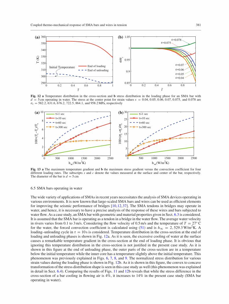
Fig. 12 a Temperature distribution in the cross-section and b stress distribution in the loading phase for an SMA bar withd = 5 cm operating in water. The stress at the center point for strain values ε = 0.04, 0.05, 0.06, 0.07, 0.075, and 0.078 areσc = 582.2, 631.6, 676.2, 722.5, 864.1, and 958.2 MPa, respectively

0 500 1000 1500 2000 25000

2

4

6

8

10

h (W/m2K)

100

(T c−

T s)/T

s

0 500 1000 1500 2000 25000

5

10

15

20

25

30

h (W/m2K)

100

(σ c−

σ s)/ σ

sτ=10 sec

τ=60 sec

τ=300 sec

τ=1 sec

τ=10 sec

τ=60 sec

τ=300 sec

τ=1 sec(a) (b)

Fig. 13 a The maximum temperature gradient and b the maximum stress gradient versus the convection coefficient for fourdifferent loading rates. The subscripts s and c denote the values measured at the surface and center of the bar, respectively.The diameter of the bar is d = 5 cm

6.5 SMA bars operating in water

The wide variety of applications of SMAs in recent years necessitates the analysis of SMA devices operating invarious environments. It is now known that large-scaled SMA bars and wires can be used as efficient elementsfor improving the seismic performance of bridges [10,12,37]. The SMA tendons in bridges may operate inwater, and hence, it is necessary to have a precise analysis of the response of these wires and bars subjected towater flow. As a case study, an SMA bar with geometric and material properties given in Sect. 6.3 is considered.It is assumed that the SMA bar is operating as a tendon in a bridge in the water flow. The average water velocityin rivers varies from 0.1 to 3 m/s. Considering the flow velocity of 0.5 m/s and the temperature of T = 27◦ Cfor the water, the forced convection coefficient is calculated using (51) and is h∞ = 2, 529.3 W/m2K. Aloading–unloading cycle in τ = 10 s is considered. Temperature distribution in the cross-section at the end ofloading and unloading phases is shown in Fig. 12a. As it is seen, the excessive cooling of water at the surfacecauses a remarkable temperature gradient in the cross-section at the end of loading phase. It is obvious thatignoring this temperature distribution in the cross-section is not justified in the present case study. As it isshown in this figure at the end of unloading phase, the outer parts of the cross-section are in a temperaturebelow the initial temperature while the inner core has a temperature slightly above the initial temperature. Thisphenomenon was previously explained in Figs. 6, 7, 8, and 9. The normalized stress distribution for variousstrain values during the loading phase is shown in Fig. 12b. As it is shown in this figure, the convex to concavetransformation of the stress distribution shape is seen in this case study as well (this phenomenon was explainedin detail in Sect. 6.4). Comparing the results of Figs. 11 and 12b reveals that while the stress difference in thecross-section of a bar cooling in flowing air is 4%, it increases to 14% in the present case study (SMA baroperating in water).


0 500 1000 1500 2000 2500 3000 35000

2

4

6

8

10

τ (sec)

h =134 W/m2K

h =234 W/m2K

h =2529 W/m2K

100

(T c−

T s)/T

s

0 500 1000 1500 2000 2500 3000 35000

5

10

15

20

25

30

τ (sec)

100

(σ c−

σ s)/σ

s

h =134 W/m2K

h =234 W/m2K

h =2529 W/m2K

(a) (b)

Fig. 14 a The maximum temperature gradient and b the maximum stress gradient versus the loading rate for three variousconvection coefficients. The subscripts s and c represent the values measured at the surface and center of bar, respectively. Thediameter of bar is d = 5 cm

10 20 30 40 500

2

4

6

8

d (mm)

Air, U =50 m/s

Air, U =100 m/s

Water, U =0.5 m/s

10 20 30 40 500

5

10

15

20

25

d (mm)

Air, U =50 m/s

Air, U =100 m/s

Water, U =0.5 m/s

100

(σ c−

σ s)/σ

s

100

(T c−

T s)/T

s

(a) (b)

Fig. 15 a The maximum temperature gradient and b the maximum stress gradient versus the bar diameter for three variousambient conditions. The subscripts s and c represent the values measured at the surface and center of bar, respectively. The totalloading–unloading time is τ =10 s

6.6 Size, boundary condition, and loading rate effects on the temperature and stress gradients

As it was shown in the previous sections, the gradients of temperature and stress in the cross-section are stronglyaffected by the ambient condition, diameter of the bar, and the loading–unloading rate. In this section, we studythe effect of these parameters on the maximum temperature and stress gradients in the cross-section of SMAbars and wires subjected to uniaxial loading. For the sake of brevity, we consider only the loading phase. Theinitial and ambient temperatures are assumed to be T0 = T∞ = 300 K for all the case studies in this section.In each case, for studying the nonuniformity in stress and temperature distributions in the cross-section, thedifference between the value of these parameters at the center and surface of the bar is nondimensionalizedby dividing by the value of the corresponding parameter at the surface. The maximum temperature and stressgradients versus the convection coefficient for four various loading rates are shown in Fig. 13. A bar withd = 5 cm and material properties similar to the previous case study is considered, and the range of convectioncoefficient is chosen to cover the free and forced convection of air, and water flow on the bar (see the casestudies in Sects. 6.3 and 6.5). As it is shown in this figure for all the loading rates, both the temperature andstress gradients increase for larger convection coefficients. However, for the slow loading rate τ = 300 sec,the increase in gradient is suppressed for convection coefficients larger than h∞ � 1, 000 W/m2K, since thematerial has enough time to exchange heat with the ambient. It is worth noting that for the slow loading rateτ =300 s, the trend of the gradient change is different from the other (fast) loading rates. We will study theeffect of changing the loading rate on the gradients in the following case study and will find the critical timecorresponding to this change of trend for some sample ambient conditions. It is shown in Fig. 13 that the


temperature and stress gradients in the cross-section are more excessive for larger convection coefficients forall the loading rates.

The effect of changing the loading rate on the maximum temperature and stress nonuniformity in thecross-section for three different convection coefficients is shown in Fig. 14. The results are presented for thetotal loading–unloading times 1 ≤ τ ≤ 3, 600 s. As it is shown, larger convection coefficients lead to morenonuniformity for both the stress and temperature distributions. Also, it is shown that for all the convectioncoefficients, the temperature and stress gradients are negligible for very fast and very slow loading rates andpeak at an intermediate loading rate (τ = 140 s for h∞ = 134 W/m2K, τ = 100 s for h∞ = 234 W/m2K,and τ = 30 s for h∞ = 2, 529 W/m2K). This is expected because for very fast loadings, the material at thesurface does not have enough time to exchange the latent heat with the ambient and the temperature and stressdistributions are almost uniform. For very slow loadings, the latent heat in the whole cross-section has enoughtime to be exchanged with the ambient and the temperature, and stress distributions are almost uniform inthe cross-section. For an intermediate loading rate, the temperature and stress distribution nonuniformity ismaximum. Also, it is worth mentioning that the loading rate corresponding to the maximum nonuniformitydecreases by increasing the convection coefficient.

The size effect on the temperature and stress nonuniformity is studied for three different ambient conditionsin Fig. 15 (the total loading–unloading time is τ = 10 s). As explained in Sect. 5, the convection coefficientdepends on the bar diameter, and for obtaining the results presented in Fig. 15, the appropriate convectioncoefficient for each diameter and ambient condition is calculated using the formulation of Sect. 5. As it isshown in Fig. 15, in the case of water flow, the temperature and stress nonuniformities are more pronouncedcompared to those of the air flow ambient condition. For the forced convection by air, the temperature andstress gradients increase for larger diameters. However, in the case of water flow, the gradients have a peak atd � 25 mm.

The results presented in Figs. 13, 14, and 15 clearly describe the complicated effect of size, ambient condi-tion, and loading rate on the coupled thermo-mechanical response of SMA bars. These figures can be used bya designer to decide whether a coupled thermo-mechanical formulation with considering the heat flux in thecross-section is necessary or using simpler lumped models is enough. It is worth mentioning that although forthe uniaxial loading of bars and wires the simpler models assuming lumped temperature in the cross-sectioncan be used with an error, there are numerous cases for which the present formulation is the only analysisoption. An example is torsion of circular SMA bars for which shear stress has a complicated nonuniform dis-tribution in the cross-section [33]. It would be incorrect to consider a lumped temperature in the cross-sectionfor torsion problems. Considering the effect of phase transformation latent heat in torsion of SMA bars is thesubject of a future communication. We have been able to show that ignoring the heat flux and the temperaturenonuniformity in the cross-section of SMA bars subjected to torsion leads to inaccurate results. It is also worthnothing that all the numerical simulations presented in this paper are performed on a 2 GHz CPU with 2 GBRAM. Since the presented explicit finite difference formulation needs a variable minimum time increment forguarantying numerical stability for various dimensions and material properties [36], the computational timevaries for different case studies. However, by considering an average of 30 nodes (for smaller diameters fewernodes are used) in the cross-section and using the material properties in Table 1, the most time-consumingcase studies (examples with large number of nodes in the cross-section and large loading–unloading times)are all completed in less than 20 min.

7 Conclusions

In this paper, a coupled thermo-mechanical framework considering the effect of generated (absorbed) latentheat during forward (reverse) phase transformation is presented for shape memory alloys. The governingequations are discretized for SMA bars and wires with circular cross-sections by considering the nonuniformtemperature distribution in the cross-section. Appropriate convective boundary conditions are used for stilland flowing air and also flowing water on slender and thick cylinders. The present formulation is capable ofsimulating the uniaxial thermo-mechanical response of SMA bars and wires by taking into account the effectof phase transformation-induced latent heat in various ambient conditions. The results of some experiments areused for evaluating the accuracy of the present formulation in modeling the rate dependency and temperaturechanges in uniaxial loading of SMA wires and bars. Several numerical examples are presented for studying theinteraction between thermo-mechanical coupling, loading rate, ambient conditions, and size of the specimen.It is shown that a loading being quasi-static strongly depends on external conditions, e.g., the size and ambient


conditions. Temperature distribution in the cross-section is also studied, and it is shown that the loading rate,ambient conditions, and size of the specimen affect the temperature distribution.

The method of this paper can be used for an accurate simulation of the material response of SMA devicesin the presence of rate dependency, size, and ambient condition effects. The present method can be exploited toanalyze SMA bars with various cross-sections. Our three-dimensional coupled thermo-mechanical formulationcan be used for studying other loadings, e.g., torsion, bending, and combined loadings. Also, the constitutiveequations used in this work can be modified to take into account the accumulated fatigue strains. These willbe the subject of future communications.

References

1. Airoldi, G., Riva, G., Rivolta, B., Vanelli, M.: DSC calibration in the study of shape memory alloys. J. Therm.Anal. 42(4), 781–791 (1994)

2. Arpaci, V.S.: Conduction Heat Transfer. Addison-Wesley, Reading (1966)3. Auricchio, F., Fugazza, D., Desroches, R.: Rate-dependent thermo-mechanical modelling of superelastic shape-memory

alloys for seismic applications. J. Intell. Mater. Syst. Struct. 19, 47–61 (2008)4. Bernardini, D., Vestroni, F.: Non-isothermal oscillations of pseudoelastic devices. Int. J. Non-Linear Mech. 38,

1297–1313 (2003)5. Birman, V.: Review of mechanics of shape memory alloy structures. Appl. Mech. Rev. 50(11), 629–645 (1997)6. Boyd, J.G., Lagoudas, D.C.: A thermodynamic constitutive model for the shape memory alloy materials. Part I. The mono-

lithic shape memory alloy. Int. J. Plast. 12, 805–842 (1996)7. Cebeci, T.: Laminar free convective heat transfer from the outer surface of a vertical slender circular cylinder. In: Proceedings

5th International Heat Transfer Conference, vol. 3, pp. 15–19. PaperNC1.4, Tokyo (1974)8. Chang, B.C., Shaw, J.A., Iadicola, M.A.: Thermodynamics of shape memory alloy wire: modeling, experiments, and appli-

cation. Contin. Mech. Thermodyn. 18, 83–118 (2006)9. Chen, Y.C., Lagoudas, D.C.: Impact induced phase transformation in shape memory alloys. J. Mech. Phys. Solids 48(2),

275–300 (2000)10. DesRoches, R., Delemont, M.: Seismic retrofit of simply supported bridges using shape memory alloys. Eng.

Struct. 24(3), 325–332 (2002)11. DesRoches, R., McCormick, J., Delemont, M.: Cyclic properties of superelastic shape memory alloy wires and bars.

J. Struct. Eng. 130(1), 38–46 (2004)12. DesRoches, R., Taftali, B., Ellingwood, B.R.: Seismic performance assessment of steel frames with shape memory alloy

connections. Part I analysis and seismic demands. J. Earthq. Eng. 14(4), 471–486 (2010)13. Fand, R.M.: Heat transfer by forced convection from a cylinder to water in crossflow. Int. J. Heat Mass Transf. 8(7),

995–1010 (1965)14. Forsythe, G.E., Malcolm, M.A., Moler, C.B.: Computer Methods for Mathematical Computations. Prentice-Hall, Upper

Saddle River (1976)15. Gall, K., Sehitoglu, H., Chumlyakov, Y.I., Kireeva, I.V.: Tension-compression asymmetry of the stress–strain response in

aged single crystal and polycrystalline NiTi. Acta Mater. 47, 1203–1217 (1999)16. Goo, B.C., Lexcellent, C.: Micromechanics-based modeling of two-way shape memory effect of a single crystalline shape

memory alloy. Acta Metall. Et Mater. 45(2), 727–737 (1997)17. Gao, X., Huang, M., Brinson, L.C.: A multivariant micromechanical model for SMAs. Part 1: crystallographic issues for

single crystal model. Int. J. Plast. 16(10–11), 1345–1369 (2000)18. He, X.M., Rong, L.J.: DSC analysis of reverse martensitic transformation in deformed Ti-Ni-Nb shape memory alloy. Scr.

Mater. 51(1), 7–11 (2004)19. Hilpert, R.: Wärmeabgabe yon geheizten drähten und rohern im lufstrom. Forsch. Geb. Ingenieurw. 4, 215–224 (1933)20. Holman, J.P. : Heat Transfer. McGraw-Hill, New York (1990)21. Iadicola, M.A., Shaw, J.A.: Rate and thermal sensitivities of unstable transformation behavior in a shape memory alloy. Int.

J. Plast. 20, 577–605 (2004)22. Knudsen, J.G., Katz, D.L.: Fluid Dynamics and Heat Transfer. McGraw-Hill, New York (1958)23. Lagoudas, D.C., Bo, Z., Qidwai, M.A.: A unifed thermodynamic constitutive model for SMA and finite element analysis of

active metal matrix composite. Mech. Compos. Mater. Struct. 3, 153–179 (1996)24. Lagoudas, D.C., Ravi-Chandar, K., Sarh, K., Popov, P.: Dynamic loading of polycrystalline shape memory alloy rods. Mech.

Mater. 35, 689–716 (2003)25. Lagoudas, D.C., Entchev, P.B.: Modeling of transformation-induced plasticity and its effect on the behavior of porous shape

memory alloys. Part I: constitutive model for fully dense SMAs. Mech. Mater. 36(9), 865–892 (2004)26. Lagoudas, D.C., Entchev, P.B., Popov, P., Patoor, E., Brinson, L.C., Gao, X.: Shape memory alloys, Part II: modeling of

polycrystals. Mech. Mater. 38, 430–462 (2006)27. Lagoudas, D.C. (ed.): Shape Memory Alloys: Modeling and Engineering Applications. Springer, New York (2008)28. Liang, C., Rogers, C.A.: The multi-dimensional constitutive relations of shape memory alloys. J. Eng. Math. 26,

429–443 (1992)29. Liu, N., Huang, W.M.: DSC study on temperature memory effect of NiTi shape memory alloy. Trans. Nonferrous Metals

Soc. China 16, s37–s41 (2006)30. McCormick, J., Tyber, J., DesRoches, R., Gall, K., Maier, H.J.: Structural engineering with NiTi. II: mechanical behavior

and scaling. J. Eng. Mech. 133(9), 1019–1029 (2007)


31. Messner, C., Werner, E.A.: Temperature distribution due to localised martensitic transformation in SMA tensile test speci-mens. Comput. Mater. Sci. 26, 95–101 (2003)

32. Mirzaeifar, R., Shakeri, M., Sadighi, M.: Nonlinear finite element formulation for analyzing shape memory alloy cylindricalpanels. Smart Mater. Struct. 18(3), 035002 (2009)

33. Mirzaeifar, R., DesRoches, R., Yavari, A.: Exact solutions for pure torsion of shape memory alloy circular bars. Mech.Mater. 42(8), 797–806 (2010)

34. Mirzaeifar, R., Shakeri, M., DesRoches, R., Yavari, A.: A semi-analytic analysis of shape memory alloy thick-walledcylinders under internal pressure. Arch. Appl. Mech. (2010). doi:10.1007/s00419-010-0468-x

35. Mirzaeifar, R., DesRoches, R., Yavari, A.: A combined analytical, numerical, and experimental study of shape-memory-alloyhelical springs. Int. J. Solids Struct. 48(3–4), 611–624 (2011)

36. Özisik, M.N.: Finite Difference Methods in Heat Transfer. CRC-Press, Boca Raton (1994)37. Padgett, J.E, DesRoches, R., Ehlinger, R.: Experimental response modification of a four-span bridge retrofit with shape

memory alloys. Struct. Control Health Monit. 17(6), 694–708 (2010)38. Paradis, A., Terriault, P., Brailovski, V.: Modeling of residual strain accumulation of NiTi shape memory alloys under

uniaxial cyclic loading. Comput. Mater. Sci. 47, 373–383 (2009)39. Patoor, E., Lagoudas, D.C., Entchev, P.B., Brinson, L.C., Gao, X.: Shape memory alloys, Part I: general properties and

modeling of single crystals. Mech. Mater. 38, 391–429 (2006)40. Popiel, C.O.: Free convection heat transfer from vertical slender cylinders: a review. Heat Transf. Eng. 29(6), 521–536 (2008)41. Qidwai, M.A., Lagoudas, D.C.: On thermomechanics and transformation surfaces of polycrystalline NiTi shape memory

alloy material. Int. J. Plast. 16, 1309–1343 (2000)42. Qidwai, M.A., Lagoudas, D.C.: Numerical implementation of a shape memory alloy thermomechanical constitutive model

using return mapping algorithms. Int. J. Numer. Methods Eng. 47, 1123–1168 (2000)43. Rajagopal, K.R., Srinivasa, A.R.: Mechanics of the inelastic behavior of materials. part I: theoretical underpinnings. Int. J.

Plast. 14(10–11), 945–967 (1998)44. Saint-Sulpice, L., Chirani, S.A., Calloch, S.: A 3D super-elastic model for shape memory alloys taking into account pro-

gressive strain under cyclic loadings. Mech. Mater. 41, 12–26 (2009)45. Simo, J.C., Hughes, T.J.R.: Computational inelasticity, vol. 7 of interdisciplinary applied mathematics. Springer, New

York (1998)46. Tanaka, K.: A thermomechanical sketch of shape memory effect: one-dimensional tensile behaviour. Res Mech. 18,

251–263 (1986)47. Tanaka, K., Kobayashi, S., Sato, Y.: Thermomechanics of transformation pseudoelasticity and shape memory effect in

alloys. Int. J. Plast. 2, 59–72 (1986)48. Tanaka, K., Nishimura, F., Hayashi, T., Tobushi, H., Lexcellent, C.: Phenomenological analysis on subloops and cyclic

behavior in shape memory alloys under mechanical and/or thermal loads. Mech. Mater. 19, 281–292 (1995)49. Tyber, J., McCormick, J., Gall, K., DesRoches, R., Maier, H., Maksoud, A.E.A.: Structural engineering with NiTi. I: basic

materials characterization. J. Eng. Mech. 133(9), 1009–1018 (2007)50. Vitiello, A., Giorleo, G., Morace, R.E.: Analysis of thermomechanical behaviour of Nitinol wires with high strain rates. Smart

Mater. Struct. 14, 215–221 (2005)

http://dx.doi.org/10.1007/s00419-010-0468-x

analysis of the rate-dependent coupled thermo-mechanical response of shape memory alloy bars and...

Documents