analysis of repeated measures data with clumping at zero

http://smm.sagepub.com/Research

Statistical Methods in Medical

http://smm.sagepub.com/content/11/4/341The online version of this article can be found at:

DOI: 10.1191/0962280202sm291ra

2002 11: 341Stat Methods Med ResJanet A Tooze, Gary K Grunwald and Richard H Jones

Analysis of repeated measures data with clumping at zero

Published by:

http://www.sagepublications.com

can be found at:Statistical Methods in Medical ResearchAdditional services and information for

http://smm.sagepub.com/cgi/alertsEmail Alerts:

http://smm.sagepub.com/subscriptionsSubscriptions:

http://www.sagepub.com/journalsReprints.navReprints:

http://www.sagepub.com/journalsPermissions.navPermissions:

http://smm.sagepub.com/content/11/4/341.refs.htmlCitations:

What is This?

- Aug 1, 2002Version of Record >>

at UNIV MASSACHUSETTS BOSTON on August 21, 2014smm.sagepub.comDownloaded from at UNIV MASSACHUSETTS BOSTON on August 21, 2014smm.sagepub.comDownloaded from

http://smm.sagepub.com/

http://smm.sagepub.com/content/11/4/341

http://www.sagepublications.com

http://smm.sagepub.com/cgi/alerts

http://smm.sagepub.com/subscriptions

http://www.sagepub.com/journalsReprints.nav

http://www.sagepub.com/journalsPermissions.nav

http://smm.sagepub.com/content/11/4/341.refs.html

http://smm.sagepub.com/content/11/4/341.full.pdf

http://online.sagepub.com/site/sphelp/vorhelp.xhtml



Analysis of repeated measures data with clumping atzeroJanet A Tooze National Cancer Institute, Bethesda, Maryland, USA, Gary K GrunwaldDepartment of Preventive Medicine and Biometrics, University of Colorado Health SciencesCenter, Denver, Colorado, USA and Richard H Jones Department of Preventive Medicineand Biometrics, University of Colorado Health Sciences Center, Denver, Colorado, USA

Longitudinal or repeated measures data with clumping at zero occur in many applications in biometrics,including health policy research, epidemiology, nutrition, and meteorology. These data exhibit correlationbecause they are measured on the same subject over time or because subjects may be considered repeatedmeasures within a larger unit such as a family. They present special challenges because of the extreme non-normality of the distributions involved. A model for repeated measures data with clumping at zero, using amixed-effects mixed-distribution model with correlated random effects, is presented. The model containscomponents to model the probability of a nonzero value and the mean of nonzero values, allowing forrepeated measurements using random effects and allowing for correlation between the two components.Methods for describing the effect of predictor variables on the probability of nonzero values, on the meanof nonzero values, and on the overall mean amount are given. This interpretation also applies to the mixed-distribution model for cross-sectional data. The proposed methods are illustrated with analyses of effects ofseveral covariates on medical expenditures in 1996 for subjects clustered within households using datafrom the Medical Expenditure Panel Survey.

1 Introduction

Data with clumping at zero commonly occur in biometrics. Typically the outcomevariable measures an amount that must be non-negative and may in some cases be zero.The positive values are generally skewed, often extremely so. Examples includeconcentrations of compounds, amounts of health or insurance expenditures, oramounts of rainfall or pollutants. Distributions of data of this type follow a commonform: there is a spike or discrete probability mass at zero, followed by a bump or rampdescribing positive values. Since the variable of interest describes an amount there isoften interest in estimating the mean amount, including zeros, perhaps in order toestimate total amounts. For example, in estimating mean per person medical expendi-tures, it must be taken into account that some subjects will have no expenditures duringthe period of interest. From these means, group totals could be estimated.

Various approaches to the problem of data clumped at zero have been proposed, butmost of them have drawbacks.1 If the data are treated as if they come from a normaldistribution, the clumping at zero is ignored as well as the tendency of the positive data

Address for correspondence: J Austin Tooze, Cancer Prevention Fellow, National Cancer Institute,Executive Plaza North, Suite 3131, 6130 Executive Blvd, MSC7354, Bethesda, MD 20892-7354, USA.E-mail: [email protected]

Statistical Methods in Medical Research 2002; 11: 341^355

# Arnold 2002 10.1191=0962280202sm291ra

at UNIV MASSACHUSETTS BOSTON on August 21, 2014smm.sagepub.comDownloaded from


to be skewed. If a nonparametric approach utilizing the distribution of the ranks isemployed, a large number of ties will exist corresponding to the zero observations, andthe distribution will not be symmetric. In addition, it is not possible to obtainpredictions of the response variable or to estimate totals using a nonparametricapproach. Another approach to analyzing data of this type is to divide the data intotwo parts—those data with a value equal to zero and those greater than zero. If only thedata greater than zero are used in the analysis, important information about subjectswith zero response is lost, and estimates of totals will not include zero values. When oneis relying on estimates from such analyses to make policy decisions, inaccurateconclusions may be made, which may lead to policies that are inadequate orinappropriate for the population of interest. In addition, this method does not accountfor the relationship that may exist between the probability of a nonzero response andthe level of the nonzero response.

The majority of the literature in the area of data that are clumped at zero addressesthe cross-sectional case where the unit of observation is measured once.1 –4 Clumping atzero may also occur with repeated measures or longitudinal data. In addition to sharingthe problems of cross-sectional data with clumping at zero, the correlation amongmeasurements on the same unit of observation must be accounted for.

We propose a mixed-distribution model based on the work of Lachenbruch1 ,2 forcross-sectional data and Grunwald and Jones5 for time series data. The model is alsosimilar to the ‘two-part model’ used for cross-sectional data in econometrics.3 ,6 All ofthese approaches combine models for the probability of occurrence of a nonzero value(a probit or logit model) and for the probability distribution of the nonzero values (alognormal or exponential family distribution). The term ‘mixed-distribution model’refers to a mixture-of-distributions model that takes the general form

f …y† ˆPr…Y ˆ 0†; if y ˆ 0‰1 ¡ Pr…Y ˆ 0†Šh…y† if y > 00 if y < 0

8<

: …1†

where h(y) is a probability density de�ned when y > 0.1 ,2 We draw on methods formodeling non-normal responses with random effects7 to incorporate random unit(subject) effects into the two parts of the model to account for the correlation due tomultiple observations made on the same subject or unit. We also allow the random uniteffects for the probability of a nonzero value and for the distribution of nonzero valuesto be correlated with each other. This allows units with higher rates of occurrence toalso have higher (or lower) mean nonzero responses. Correlation between the randomeffects in the two model components is similar to the cross-sectional correlationbetween the random normal errors in the two model components of the Heckman,or Type II Tobit model.8

Section 2 outlines the proposed mixed-distribution model for longitudinal data withcorrelated random effects, shows how the methods of generalized linear mixed models(GLMM) and nonlinear mixed models may be used to �t the model, and addresses theinterpretation of the model parameters in terms of the total amount, including zeros. Inparticular, a covariate may affect the mean amount by affecting both the probability of

342 JA Tooze et al.



occurrence of a nonzero value and also the mean of the nonzero values, and we give anapproach to quantifying and separating these two effects. In Section 3, results fromsimulation studies are presented. Section 4 illustra tes application of the mixed-distribu-tion model for repeated measures data using data from the Medical Expenditure PanelSurvey, and Section 5 provides a summary and discusses areas for further research.

2 Mixed-distribution model with correlated random e¡ects

In this section a mixed-distribution model for repeated measures data with clumping atzero and correlated random effects is introduced. This model will be referred to as thecorrelated mixed-distribution model. An extension of the mixed-distribution model waschosen to model repeated measures data because it provides a general statisticalmodeling approach using existing methodologies (generalized linear and nonlinearmixed-effects models). The model gives information about the separate occurrence andnonzero amount components of the model as well as the overall mean. The correlatedmixed-distribution model relates the two components of the model by assuming abivariate normal distribution for the random effects.

2.1 ModelFor a random variable Yij, which represents the amount of a quantity with observed

value yij for a unit of observation i at time j, let Rij represent the occurrence variablewhere

Rij ˆ 0; if Yij ˆ 01; if Yij > 0

»

Rij has conditional probabilities

Pr…Rij ˆ rij j q1† ˆ 1 ¡ pij…q1†; if rij ˆ 0p ij…q1†; if rij ˆ 1

»

where q1 ˆ ‰b01 ; u1iŠ0 is a vector of �xed occurrence effects b1 , and random unit

occurrence effect u1 i. We assume a logistic model for occurrence so that

logit…pij…q1†† ˆ X01ijb1 ‡ u1i …2†

where X1 ij is a vector of covariates for occurrence.De�ne Sij ² ‰Yij j Rij ˆ 1Š to be the intensity variable with p.d.f. f …sijjq2† for sij > 0

and mean E…Sijjq2† ˆ ms ij…q2† where q2 ˆ ‰b0

2 ; u2iŠ0 is a vector of �xed intensity effects b2and random unit intensity effect u2i. We assume a lognormal model for intensity so that

log…Sij j q2† ¹ N…X02ijb2 ‡ u2i; s2

e † …3†

Analysis of repeated measures data with clumping at zero 343



where X2 ij is a vector of covariates for intensity. We allow the random effects foroccurrence and intensity to be correlated by assuming that

u1iu2i

µ ¶¹ BVN

00

µ ¶;

s21 rs1s2

rs1s2 s22

µ ¶³ ´: …4†

Under this assumption the subject-speci�c mean intensity is

E…Sij j q2† ˆ exp X02ijb2 ‡ u2i ‡ s2

e

2

³ ´…5†

and the marginal mean intensity is

E…Sij j b2† ˆ exp X02ijb2 ‡ s2

2

2‡ s2

e

2

³ ´…6†

Note in particular that the values and interpretations of the �xed effects parametersb2 are identical in (5) and (6) except for the intercept.7

The p.d.f. of Yij is

f …yij j q† ˆ Pr…Rij ˆ 0 j q1†d0…yij† ‡ Pr…Rij ˆ 1 j q1†f …s ij j q2†ˆ ‰1 ¡ pij…q1†Šd0…yij† ‡ pij…q1†f …sij j q2†

where q ˆ ‰q01; q0

2Š and d0…y† is a Dirac delta function9 such that

„ 1¡1 d0…y†dyij ˆ 1

d0…y† ˆ 0 when yij 6ˆ 0

»

The conditional expectation of Yij is:

E…Yij j q† ˆ pij…q1†mSij…q2†; …7†

and the conditional variance is:1 0

var…Yij j q† ˆ pij…q1†var…Sij j q2† ‡ …pij…q1††‰1 ¡ …pij…q1††ŠmSij…q2†2 :

The contribution to the likelihood for the ith subject (i ˆ 1, . . . , m) is

Li…b1 ; b2 ; s1; s2 ; se; r; yi1; . . . ; yini†

ˆ…

u1 i

…

u2i

Yn1

jˆ1

f …yij j b1; b2 ; u1i; u2i†f …u1i; u2i j s1; s2 ; se; r†du1idu2i:

344 JA Tooze et al.



The likelihood is then

L…b1 ; b2 ; s1 ; s2; se; r† ˆYm

iˆ1

…

u1 i

…

u2 i

Yni

jˆ1

f …yij j b1 ; b2; u1i; u2i†f …u1i; u2i js1 ; s2; se; r†du1idu2i

ˆYm

iˆ1

…

u1i

…

u2i

Yni

jˆ1

‰1 ¡ pij…b1; u1i†Š1¡rij ‰pij…b1 ; u1i†Šrij

£ f …sij j b2 ; u2i†f …u1i; u2i j s1 ; s2 ; se; r†du1idu2i …8†

In the correlated mixed-distribution model, it is not assumed that the random effectsare independent and, as a result, the components of (8) for occurrence and intensitycontain a common parameter, r. Therefore, the two components of the likelihoodcannot be maximized separately as in Lachenbruch2 or Grunwald and Jones.5 In model(8) it is also possible for b1 and b2 to share common parameters. However, because b1and b2 are on different scales, doing so may lead to parameter estimates that aredif�cult to interpret.

With the assumptions that u1 i and u2 i are independent, i.e. that r ˆ 0, the likelihoodmay be factored into two parts that correspond to the occurrence process and theintensity process:

L…b1; b2; s1 ; s2 ; se† ˆYm

iˆ1

…

u1i

Yni

jˆ1

‰1 ¡ pij…q1†Š1¡rij ‰p ij…q1†Šrijf …u1i j s1†du1i

£Ym

iˆ1

…

u2i

Yni

jˆ1

f …sij j q2†f …u2i j s2; se†du2i

The �rst component is the likelihood for the occurrence process, LR…b1; s1†, and thesecond component is the likelihood for the intensity process, LS…b2; s2; se†. With thefurther assumption that q1 has no parameters in common with q2 , L…b1 ; b2 ; s1 ; s2; se† ismaximized when each component is maximized separately. When r ˆ 0, the model isreferred to as the uncorrelated mixed-distribution model.

2.2 Model ¢ttingIf u1 i and u2 i are assumed to be independent, then maximum likelihood methods may

be used to maximize both components of the likelihood separately. Wol�nger andO’Connell’s pseudo-likelihood approach,1 1 Breslow and Clayton’s penalized quasi-likelihood approach,1 2 or optimization of the likelihood approximated by adaptiveGaussian quadrature,1 3 may be used to maximize LR…b1 ; s1† and LS…b2 ; s2 ; se† sepa-rately. The overall likelihood L…b1 ; b2 ; s1; s2; se† is the product of LR…b1 ; s1† andLS…b2 ; s2 ; se†, and the maximum of L…b1; b2 ; s1 ; s2 ; se† occurs when LR…b1 ; s1† andLS…b2 ; s2 ; se† are maximized separately. If the models contain no random effects, thisallows the mixed-distribution model to be estimated using standard software ofgeneralized linear models1 4 . When correlated random effects are present these specialcases are useful for obtaining initia l estimates when optimizing the correlated modellikelihood (8).




The full likelihood (8) for the correlated mixed-distribution model can be maximizedusing quasi-Newton optimization of a likelihood approximated by adaptive Gaussianquadrature.1 3 This method is implemented in the SAS PROC NLMIXED procedure (SASInstitute, Cary, NC, Version 8). This procedure allows the user to specify a generallikelihood, in particular one of the form (8), and also allows great �exibility forspeci�cation of the distribution of Sij. We assume a logistic-lognormal-normal model,where ‘logistic’ refers to the modeling of the occurrence part of the model (2), ‘lognormal’to the modeling of the intensity part of the model (3), and ‘normal’ to the assumption thatthe random effects are assumed to have a bivariate normal distribution (4).

To �t this model we developed a SAS macro (MIXCORR, available from theauthors) that calls PROC GENMOD and PROC NLMIXED. The user must specify thedataset, the outcome variable, covariates for the binomial component of the model andfor the lognormal component of the model, and the variable that identi�es the randomunit. The macro estimates a binomial model for the occurrence and a lognormal modelfor the intensity (both without random effects) using PROC GENMOD. Theseparameter estimates are used as starting values in estimating the separate occurrenceand intensity models with uncorrelated random effects using SAS PROC NLMIXED.Finally, the parameter estimates from the two uncorrelated random effects models areused as starting values for the mixed-distribution model with correlated random effectsin a �nal PROC NLMIXED run. The starting value for the covariance of the randomeffects is calculated using the estimates of s2

1 and s22 and r ˆ 0.5.

2.3 Model checkingThe model assumes normality and constant variance of random effects, m1i and m2i,

and the residuals of the intensity distribution. Standard regression diagnostics may beused to assess the goodness of �t of the model. Quantile–quantile plots can beconstructed for uu1i and uu2i, and for the residuals for the intensity variable, given byln…s ij† ¡ …X0

2ijb2 ‡ u2i†. If the normality assumption is not violated, the data will fall in astraight line. A plot of the residuals for the intensity distribution versus �tted values willindicate if the assumption of constant variance is violated. A nonrandom patternindicates departure from this assumption.

2.4 Interpretation of Fixed-E¡ects ParametersThe separate effects of the �xed-effect occurrence and intensity parameters, b1 and

b2 , have the same interpretations for occurrence and intensity as they would have if thetwo components of the model were �t separately (e.g., logistic and lognormal regres-sion). If a variable is used in both the occurrence and intensity models, however, theremay be interest in quantifying the overall effect of the variable on the total amount Y.This can be carried out as follows.

Assume that Z is a covariate in both the occurrence and intensity models (2) and (3),and that X1 and X2 are vectors of the other occurrence and intensity covariates,respectively. For simplicity we suppress the subscripts i and j. Then from (2) and (3),

Pr…R ˆ 1 j q1† ˆ exp…X01b1 ‡ a1z ‡ u1†

1 ‡ exp…X01b1 ‡ a1z ‡ u1† …9†

346 JA Tooze et al.



and

E…S j q2† ˆ exp X02b2 ‡ a2z ‡ u2 ‡ s2

e

2

³ ´: …10†

Then the ratio of mean amount of Y when Z ˆ z ‡ 1 to that when Z ˆ z is

E…Y j Z ˆ z ‡ 1; q†E…Y j Z ˆ z; q† ˆ Pr…R ˆ 1 j Z ˆ z ‡ 1; q1†

Pr…R ˆ 1 j Z ˆ z; q1†

µ ¶E…S j Z ˆ z ‡ 1; q2†

E…S j Z ˆ z; q2†

µ ¶…11†

From (10) the second term in (11) is exp…a2†. In general the �rst term in (11) depends onX0

1b1 ‡ u1 as well as on a1 and z. However, some insight can be gained by substituting(9) into (11) and noting that the function

exp…k ‡ a1†1 ‡ exp…k ‡ a1†

³ ´¿exp…k†

1 ‡ exp…k†

³ ´! 1 as k ! 1

and

exp…k ‡ a1†1 ‡ exp…k ‡ a1†

³ ´¿exp…k†

1 ‡ exp…k†

³ ´! exp…a1† as k ! ¡1:

Thus in (11),

E…Y j Z ˆ z ‡ 1; q†E…Y j Z ˆ z; q† º exp…a2† when X0

1b1 ‡ u1 is large and positiveexp…a1†exp…a2† when X0

1b1 ‡ u1 is large and negative

»

When X01b1 ‡ u1 is large and positive, Pr(R ˆ 1) º 1 so there are few zeros,

E(Y) º E(S), and the effect of Z on Y is mainly via the mean of the nonzero values.When X0

1b1 ‡ u1 is large and negative, the ratio of means in (11) is a combinationof occurrence and intensity effects. The term Pr…R ˆ 1 j Z ˆ z ‡ 1; q1†=Pr…R ˆ 1 jZ ˆ z; q1† is the risk ratio for occurrence per one unit change in Z. When Pr(R ˆ 1) º 0, as when X0

1b1 ‡ u1 is large and negative, this term is close to the oddsratio for occurrence per one unit change in Z, which is exp…a1† as in the usual logisticregression interpretation. Special cases of all of these results hold if Z enters into onlythe occurrence model …a2 ˆ 0† or only into the intensity model …a1 ˆ 0†.

In practice, neither of the limiting cases of (11) may apply. In order to determine therange of the effect of a common covariate Z on Y, the ratio of the means in (11) can becomputed for the minimum, maximum, and median values of Z, and for the minimumand maximum values of the other covariates. The limit exp…a1†exp…a2† in (11) providesan upper (lower) limit for the combined effect of Z on Y when a1 is positive (negative).Note that these results also hold when no random effects are present and thus providean interpretation of the combined effect of a variable in a mixed-distribution regressionmodel.




2.5 Interpretation of random e¡ectsThe random effects in the correlated mixed-distribution model, u1 i and u2 i, account

for unobserved heterogeneity among units. In the occurrence part of the model, therandom intercept on the link (e.g., logit) scale, b10i ˆ b10 ‡ u1i, allows some units tohave a consistently low or high probability of a nonzero response. The variance of therandom effect, s2

1 , indicates the variability of the probability of a nonzero responseamong units with similar covariate patterns. The random intercept, b20i ˆ b20 ‡ u2i, inthe intensity part of the model, allows some units to have consistently low or high meanof nonzero values. If s2

2 is large it indicates that there is a great deal of heterogeneity ofmean nonzero responses among units with similar covariate patterns.

Allowing correlation of the random effects u1 i and u2 i allows units with consistentlyhigh occurrence probability to have consistently high (low) mean of nonzero valueswhen the correlation between u1 i and u2 i, r, is positive (negative).

3 Simulation results

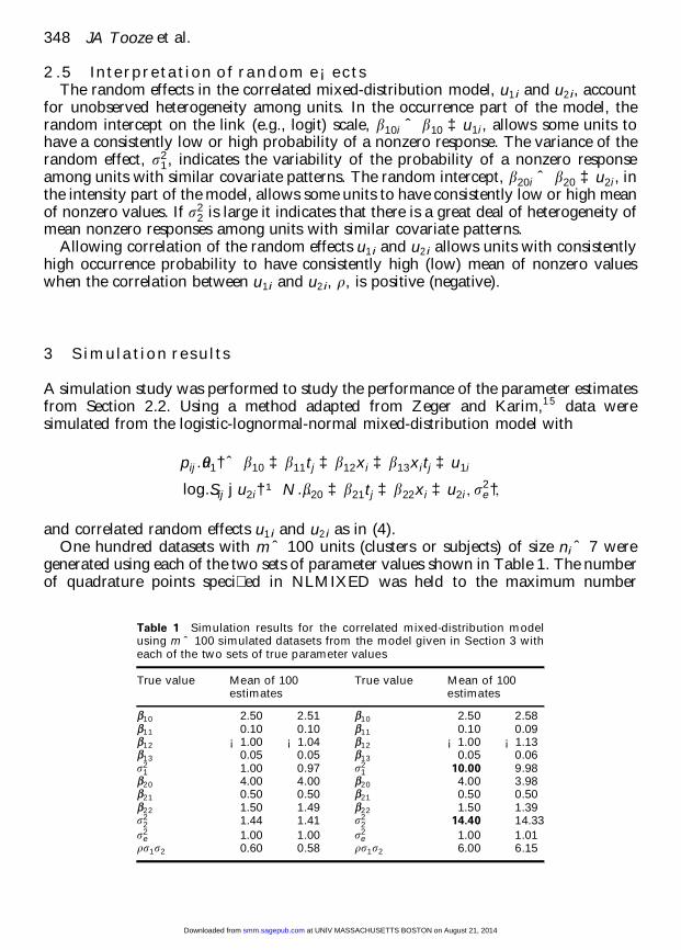
A simulation study was performed to study the performance of the parameter estimatesfrom Section 2.2. Using a method adapted from Zeger and Karim,1 5 data weresimulated from the logistic-lognormal-normal mixed-distribution model with

pij…q1† ˆ b10 ‡ b11tj ‡ b12xi ‡ b13xitj ‡ u1i

log…Sij j u2i† ¹ N…b20 ‡ b21tj ‡ b22xi ‡ u2i; s2e †;

and correlated random effects u1 i and u2 i as in (4).One hundred datasets with m ˆ 100 units (clusters or subjects) of size ni ˆ 7 were

generated using each of the two sets of parameter values shown in Table 1. The numberof quadrature points speci�ed in NLMIXED was held to the maximum number

Table 1 Simulation results for the correlated mixed-distribution modelusing m ˆ 100 simulated datasets from the model given in Section 3 witheach of the two sets of true parameter values

True value Mean of 100estimates

True value Mean of 100estimates

b10 2.50 2.51 b10 2.50 2.58b11 0.10 0.10 b11 0.10 0.09b12 ¡1.00 ¡1.04 b12 ¡1.00 ¡1.13b13 0.05 0.05 b13 0.05 0.06s2

1 1.00 0.97 s21 10.00 9.98

b20 4.00 4.00 b20 4.00 3.98b21 0.50 0.50 b21 0.50 0.50b22 1.50 1.49 b22 1.50 1.39s2

2 1.44 1.41 s22 14.40 14.33

s2e 1.00 1.00 s2

e 1.00 1.01rs1s2 0.60 0.58 rs1s2 6.00 6.15

348 JA Tooze et al.



determined adaptively, seven. The estimates from NLMIXED appear to be unbiased(Table 1).

4 Application

The Medical Expenditure Panel Survey (MEPS) is a longitudinal survey conducted bythe Agency for Healthcare Research and Quality (AHRQ) and the National Center forHealth Statistics (NCHS). MEPS data may be used to obtain estimates of health careuse, medical expenditures, and insurance coverage in the United States. In the House-hold Component of the MEPS, data were collected on health care use and expenditures,demographic characteristics, medical conditions, health status, and insurance coverageon 22 601 persons in 10 596 households. Although the expenditure and use data arecollected longitudinally, they are aggregated by year; only data for 1996 were analyzed.However, due to the multiple subjects within households, these data exhibit clustering,and the techniques described in this paper are applicable with household as the unit ofrepeated measurement. Although the MEPS is a representative sample and weightedand unweighted frequencies are provided in order to provide data analysts the ability tomake population-level estimates, the analysis presented in this paper was not weighted.

For this analysis, the impact of age, sex, health rating, the presence of a medicalcondition, census region (Northeast, Midwest, South, West), the presence of physicallimitations, and insurance status on total medical expenditures in 1996 were modeled.The health rating was assessed on a scale of 1 to 5 with 1 corresponding to ‘Excellent’and 5 corresponding to ‘Poor’. Whether or not a subject had a medical condition wasbased on household-reported medical conditions collected in 1996. A subject wasconsidered to have a limitation if they were found to have any type of limitation withactivities of daily living (ADLs: including bathing, dressing, and getting around thehouse), instrumental activities of daily living (IADLs: including using the telephone,paying bills, taking medications, preparing light meals, doing laundry, and goingshopping), physical limitations (such as walking, climbing stairs, grasping objects,reaching overhead, lifting, bending or stooping, and standing for long periods of time),any limitation that impeded their work, housework, or school activities, or vision orhearing limitations. The presence or absence of any insurance (including coverage underCHAMPUS=CHAMPVA, Medicare, Medicaid or other public hospital=physician orprivate hospital=physician insurance) was reported for each month in 1996. Theportion of the year that the respondent was insured was used as a covariate in theanalysis. There were from one to fourteen persons in a family; the median number offamily members was three. Owing to missing data on the limitation, health ratingvariable, insurance status, region, age, or sex, 746 respondents were excluded from theanalysis.

Both models with and without correlated random effects were �t using theMIXCORR macro and a backwards selection procedure. In all cases the model withcorrelated random effects was found to be better than the model with uncorrelatedrandom effects (based on a likelihood ratio test and AIC). A model with all covariateswas the best of the models considered. Parameter estimates from the models withuncorrelated and correlated random effects are given in Table 2.




Checks of the goodness of �t of the model, as described in Section 2.3, wereperformed. The quantile–quantile plots for the random effects showed no indicationof departure from a straight line. Plots of residuals versus �tted values for the lognormalintensity model did not show any indications of heteroscedasticity of variance.

The separate and combined effects of the variables included in the model arepresented in Table 3. In this table each column is referenced by a lower case letter.Recall that from (11) the ratio of the overall mean for a one unit change in a commoncovariate Z may be represented as follows:

E…Y j Z ˆ z ‡ 1†E…Y j Z ˆ z†

µ ¶

"…k†

ˆ exp…a2†"…j†

exp…a1†"

…h†

Pr…R ˆ 0 j Z ˆ z ‡ 1†Pr…R ˆ 0 j Z ˆ z†

µ ¶

"…g†|‚‚‚‚‚‚‚‚‚‚‚‚‚‚‚‚‚‚‚‚‚‚‚‚‚‚‚‚‚{z‚‚‚‚‚‚‚‚‚‚‚‚‚‚‚‚‚‚‚‚‚‚‚‚‚‚‚‚‚}

…i†

…12†

Table 2 Parameter estimates and model comparisons for � nal model � t to MEPS data

Parameter Uncorrelated Correlated

Estimate (S.E.) p > j t j Estimate (S.E) p > j t j

Occurrence (Logistic)Intercept ¡2.8292(0.1129) < 0.0001 ¡2.8131(0.1129) < 0.0001Medical condition (N ˆ 0=Y ˆ 1) 3.0342(0.0724) < 0.0001 2.9792(0.0717) < 0.0001Limitations (N ˆ 0=Y ˆ 1) 0.5574(0.0894) < 0.0001 0.5498(0.0897) < 0.0001Portion of year insured (0–1) 1.7152(0.0680) < 0.0001 1.7262(0.0679) < 0.0001Age (years) 0.0051(0.0014) 0.0003 0.0040(0.0014) 0.0043Health rating (1–5) 0.1782(0.0292) < 0.0001 0.2181(0.0296) < 0.0001Sex (M ˆ0=F ˆ 1) 0.6122(0.0509) < 0.0001 0.6318(0.0510) < 0.0001Region 1 (Northeast) 0.5173(0.0881) < 0.0001 0.5184(0.0884) < 0.0001Region 2 (Midwest) 0.5547(0.0867) < 0.0001 0.5465(0.0869) < 0.0001Region 3 (South) 0.1359(0.0724) 0.0606 0.1236(0.0726) 0.0886s2

1 1.1502(0.1140) < 0.0001 1.1852(0.1149) < 0.0001

Intensity (Lognormal)

Intercept 3.0459(0.0619) < 0.0001 2.8653(0.0641) < 0.0001Medical condition (N ˆ 0=Y ˆ 1) 1.0485(0.0473) < 0.0001 1.1503(0.0482) < 0.0001Limitations (N ˆ 0=Y ˆ 1) 0.5681(0.0299) < 0.0001 0.5743(0.0299) < 0.0001Portion of year insured (0–1) 0.8702(0.0347) < 0.0001 0.9047(0.0348) < 0.0001Age (years) 0.0189(0.0005) < 0.0001 0.0187(0.0005) < 0.0001Health rating (1–5) 0.2609(0.0111) < 0.0001 0.2697(0.0112) < 0.0001Sex (M ˆ0=F ˆ 1) 0.2235(0.0206) < 0.0001 0.2366(0.0206) < 0.0001Region 1 (Northeast) 0.1188(0.0355) 0.0008 0.1237(0.0356) 0.0005Region 2 (Midwest) 0.1314(0.0341) 0.0001 0.1383(0.0342) < 0.0001Region 3 (South) 0.0126(0.0313) 0.6878 0.0145(0.0313) 0.6435s2

e 1.6959(0.0239) < 0.0001 1.6960(0.0238) < 0.0001s2

2 0.2368(0.0190) < 0.0001 0.2468(0.0192) < 0.0001rs1s2 — — 0.3523(0.0347) < 0.0001

(r ˆ 0.6514)

Name Value Value Difference in ¡2 loglikelihood

AIC 293 107.6 293 002.0¡2 ll 293 061.6 292 954.0 107.59

(p < 0.0001)

350 JA Tooze et al.



Tab

le3

Eff

ects

on

med

ical

exp

end

itu

rein

1996

ME

PS

dat

afo

rco

vari

ates

(a–f

)o

np

rob

abili

tyo

fo

ccu

rren

ce(i

),o

nin

ten

sity

(j),

and

on

mea

nam

ou

nt

(k)

Var

iab

le(a

)(b

)(c

)(d

)(e

)(f

)(g

)(h

)(i

)(j)

(k)

Med

ical

con

dit

ion

Lim

itati

on

Hea

lth

ratin

gS

exIn

sura

nce

Reg

ion

Rat

ioo

fP

rob

.*e

a 1e

a 1*

ratio

(f)

ea 2

Rat

ioo

fm

ean

s

An

ym

edic

alco

nd

itio

nN

= YN

Ex

M0

40.

404

19.6

727.

946

3.15

925

.101

(Nˆ

0=Y

ˆ1)

N= Y

YP

oo

rF

12

0.05

819

.672

1.14

53.

159

3.61

7

An

ylim

itatio

nN

N= Y

Ex

M0

40.

945

1.73

31.

638

1.77

62.

909

(Nˆ

0=Y

ˆ1)

YN

= YP

oo

rF

12

0.58

01.

733

1.00

61.

776

1.78

6

Hea

lth

ratin

g(1

ˆE

x,2

ˆV

ery

NN

Ex=

VG

M0

40.

981

1.24

41.

220

1.31

01.

598

Go

od

,3

ˆG

oo

d,

4ˆ

Fair

,5

ˆP

oo

r)Y

YE

x=V

GF

12

0.80

71.

244

1.00

41.

310

1.31

4

Sex

(Mˆ

0=F

ˆ1)

NN

Ex

M= F

04

0.93

51.

881

1.75

91.

267

2.22

8Y

YP

oo

rM

= F1

20.

535

1.88

11.

007

1.26

71.

276

Po

rtio

no

fye

arin

sure

d(0

–1)

NN

Ex

M0=

14

0.73

35.

619

4.11

62.

471

10.1

72Y

YP

oo

rF

0=1

20.

184

5.61

91.

036

2.47

12.

560

Reg

ion

(1ˆ

No

rth

east

,N

NE

xM

04=

20.

946

1.72

71.

633

1.14

81.

876

2ˆ

Mid

wes

t,3

ˆS

out

h,

4ˆ

Wes

t)Y

YP

oo

rF

14=

20.

582

1.72

71.

006

1.14

81.

155

*Ag

ese

teq

ual

toth

em

ean

,34

.8ye

ars.

Ex

ˆex

celle

nt,

VG

ˆve

ryg

oo

d.

Th

ete

rms

are

asg

iven

ineq

uat

ion

(12)

.




The variable listed in the �rst column of Table 3 is z in the equation. Because thevalues of the other variables in the model impact the ratio of probabilities (g), variousscenarios for values of the other variables are given in columns (a)–(f). In general, the‘low’ condition, in which the other covariates in the model are at their lowest value, isgiven on the �rst row for the variable, and the ‘high’ condition, in which the othercovariates in the model are at their highest value, is given on the following row.

Presence of a medical condition was associated with increased mean medicalexpenditure in 1996. The increase ranged from 3.6 times (for subjects with otherwise‘high risk’ covariate patterns) to 25.1 times (for subjects with otherwise ‘low risk’covariate patterns). Differences in this effect were due to differences in the effect of amedical condition on the probability of some medical expenditure. The mean medicalexpenditure for respondents with a physical limitation was from 1.8 to almost 3 timesthe mean of respondents without physical limitations. Having insurance for the entireyear was associated with increased mean medical expenditures from 2.5 to 10.2 timesthat of persons who did not have insurance for the entire year, with the larger increasefor patients with an otherwise low risk covariate pattern. A one unit increase in thehealth rating scale, which actually corresponded to a decline in health, increased themean amount of health expenditures by 1.3 to 1.6 times. The difference between a malesubject and a similar female increased the mean amount of expenditure from 1.3 to 2.2times. Lastly, living in the Midwest increased the mean amount of expenditure from 1.2to 1.9 times that of those living in the West. In none of these cases was there a uniformdominance of the occurrence effect over the intensity effect (or vice versa) on totalexpenditure.

The signi�cant random effects variance for the occurrence shows that after account-ing for covariate differences among subjects, some families have a greater probability ofseeking medical care than others. Similarly, the highly signi�cant random effectvariance for intensity indicates that after accounting for covariate differences, somefamilies have consistently higher (or lower) expenditures when they do seek medicalcare than the norm. The positive correlation between the occurrence and intensityrandom effects indicates that after accounting for covariate differences, families with agreater tendency to seek medical care tended also to report a higher mean amount ofpositive expenditures.

5 Discussion

We have proposed a model for longitudinal or repeated measures data with clumping atzero, using a mixed-effects, mixed-distribution model. The model includes features ofthe cross-sectional statistica l models of Lachenbruch,1 ,2 the cross-sectional econometricmodels of Heckman,8 Duan et al.,3 and Manning et al.,6 and the time series model ofGrunwald and Jones.5 In addition, by including correlated random errors, the occur-rence and intensity parts of the model are linked. An interpretation of �xed-effectsparameters was given, which also applies to mixed-distribution models for cross-sectional data.

We have shown how the proposed model may be estimated using standard softwarefor non-linear and generalized linear mixed models such as SAS PROC NLMIXED.

352 JA Tooze et al.



Simulations indicate that this method of estimation gives unbiased results for both �xedand random effects. We chose this method due to its good performance on simulationstudies, and because it can be easily implemented in SAS. However, other methods ofmodel �tting appropriate for GLMMs and nonlinear mixed-effects models1 3 potentiallycould be used to �t our model, including penalized quasi-likelihood1 2 or a MonteCarlo method within a Bayesian framework.1 5

We used the approach to model the association between several covariates includingdemographic characteristics, insurance coverage, and health status on health careexpenditures of subjects, using random effects to account for clustering of subjectsinto families. We noted strong �xed effects of most covariates on total amount ofexpenditure, through both the probability of nonzero expenditure and the mean ofnonzero expenditures. We also noted strong random effects due to clustering of subjectswithin families. Further, adjusting for covariates, there was a tendency for subjects infamilies that had a higher probability of some health care expenditure to also havehigher mean nonzero expenditure.

The model proposed in this paper is appropriate for data with true zeros. Althoughthis method may appear to be applicable to the case where data are left censored ormissing, a zero in these cases is not a real zero and should not be treated as such whencalculating the mean amount.

One byproduct of our work is a method for interpreting effects of covariates.Estimation of the mean amount, including the probability of zeros, is in our viewone of the main reasons for developing models for the combined response when zerosare included. Totals, such as total expenditure for a group over a period of timeincluding the fact that some subjects will have no expenditures, can be estimated fromthese means. The method we propose gives information about the effect of a covariateon this mean amount and how that effect arises as a combination of the covariate’seffect on occurrence probability and on mean nonzero amount. The methods wepropose are also applicable in the cross-sectional case.

Many modi�cations and extensions of our methods are possible. Some types of datawith clumping at zero may exhibit serial correlation, particularly if repeated measure-ments are made longitudinally. One possible extension of the model described in thispaper is to a transition model or an autoregressive error structure to account for thetype of autoregressive pattern that longitudinal data might exhibit. Another directionfor extension would be toward the Heckman8 econometric model, which uses corre-lated random errors to allow the probability of occurrence and the mean intensity to berelated in a cross-sectional model. We have adapted that approach to include correlatedrandom unit effects, our main interest. Our model could be modi�ed to includecorrelated within-subject random components as well. Such a model could again beestimated using standard methods for GLMMs and SAS PROC NLMIXED. Furtherextensions might include both a transition component and a random effect. Otherextensions of the correlation structure, such as a stochastic parameter model includingrandom slopes as well as random intercepts, would be possible as well. However, as thecorrelation structures become more complex and additional parameters are added tothe model, the model becomes less parsimonious and more dif�cult to �t.

In this paper we have assumed that the nonzero amounts follow a lognormaldistribution, as in the two-part models of Duan et al.3 This distribution is appropriate




for skewed, positive, continuous data and is frequently used for analysis of cost data.The gamma distribution would be an alternative choice for the intensity distribution,as in Grunwald and Jones5 and Hyndman and Grunwald.1 6 The Weibull distributioncould also be chosen. All of these are distributions on (0, 1) and can be accom-modated by the model. Because all of these distributions are capable of modeling avariety of positively skewed shapes, the exact form assumed for the errors would notbe expected to have a substantial effect on the estimated model parameters orinferences. However, if quantiles of the nonzero amounts are to be estimated (as inGrunwald and Jones5 ), more care is needed to specify and check the form of the errordistribution. A nonparametric density estimate1 7 could also be considered for estimat-ing the shape of the error distribution. This approach potentially could provide betterestimation of quantiles, although sparse data in the tails of the highly skeweddistributions may cause dif�culties. We are not aware of any applications of nonpara-metric density estimation to data with clumping. Some care would be needed so thatthe estimates were applied only to the nonzero data rather than smoothing across thezeros as well. It is unclear how multiple covariates and random effects could beincluded.

In our model, an intensity model appropriate for yi> 0 was chosen so that it maybe assumed that zeros only arise when ri ˆ 0. Otherwise, it is unknown whether thezeros arise from the distribution for the occurrence component of the model, or fromthe intensity component of the model. An example of a mixture of distributions thatcontains both type of zeros is a Binomial–Poisson mixture. Lambert1 8 has proposedzero-in�ated Poisson (ZIP) regression for handling data that arise from this mixtureof distributions. Dunson and Haseman1 9 extended ZIP regression to a transitionmodel for longitudinal data with an application to carcinogenicity in animal studies.Hall2 0 adapted Lambert’s methodology to an upper-bounded count situation byusing a zero-in�ated binomial model. He also incorporated random effects into theZIP regression model to accommodate repeated measures data. Our model wasdeveloped for the case where the nonzero data arise from a continuous distribution.The Poisson would not be an appropriate distribution for the intensity variablefor the medical expenditure data described in this paper, as these data are notindependent counts.

In the econometric literature there has been an increased interest in semiparametricapproaches to �tting data with clumping at zero.2 1 ,2 2 In addition, Hyndman andGrunwald1 6 have developed a generalized additive mixed-distribution model with a�rst-order Markov structure for time series data. Another extension to the modeldescribed in this paper could involve a semiparametric modeling approach.

Because the correlated mixed-distribution model is a nonlinear model that incorpo-rates the models and methods of GLMMs, as the methodology advances in the area ofnonlinear models and GLMMs, especially with regard to model �tting and diagnostics,the methodology of the correlated mixed-distribution model will be advanced as well.

AcknowledgmentsThis research was partially supported by the National Institute of General Medical

Studies, Grant GM38519 (RHJ). The authors would also like to acknowledge Dr. GaryZerbe, Dr. David Young and Dr. Becki Bucher Bartelson for their guidance with this

354 JA Tooze et al.



research. Dr. Tooze is a fellow in the National Cancer Institute’s Cancer PreventionFellowship Program in the Division of Cancer Prevention.

References

1 Lachenbruch P. Analysis of data withclumping at zero. Biometrische Zeitschrift1976; 18: 351–56.

2 Lachenbruch P. Utility of regression analysis inepidemiologic studies of the elderly.In: Wallace R, Woolson R, eds. Theepidemiologic study of the elderly. OxfordUniversity Press, 1992.

3 Duan N, Manning WG, Morris CN,Newhouse JP. A comparison of alternativemodels for the demand for medical care. SantaMonica, California: The RAND Corporation,1982. R-2754-HHS.

4 Amemiya T. Advanced econometrics.Cambridge, Massachusetts: HarvardUniversity Press, 1985.

5 Grunwald GK, Jones RH. Markov models fortime series with mixed distribution.Environmetrics 2000; 11: 327–39.

6 Manning W, Duan N, Rogers W. MonteCarlo evidence on the choice between sampleselection and two-part models. Journal ofEconometrics 1987; 35: 59–82.

7 Diggle PJ, Liang K-Y, Zeger SL. Analysis oflongitudinal data. Oxford: Oxford UniversityPress, 1994.

8 Heckman JJ. The common structure ofstatistical models of truncation, sampleselection, and limited dependent variables anda simple estimator of such models. Annals ofEconomic and Social Measurement 1976;5: 475–92.

9 Robertson JS, Bolinger K, Glasser LM, SloaneNJ, Gross R. Chapter 1. In: Zwillinger D, ed.CRC standard mathematical tables andformulae. Boca Raton: CRC Press, 1996: 71.

10 Aitchinson J. On the distribution of a positiverandom variable having a discrete probabilitymass at the origin. Journal of the AmericanStatistical Association 1955; 50: 901–8.

11 Wol�nger R, O’Connell M. Generalized linearmodels. Journal of Statistical ComputerSimulation 1993; 48: 233–43.

12 Breslow N, Clayton D. Approximate inferencein generalized linear models. Journal of theAmerican Statistical Association 1993; 88:9–25.

13 Pinheiro JC, Bates DM. Approximations tothe log-likelihood function in the nonlinearmixed-effects model. Journal ofComputational and Graphical Statistics 1995;4: 12–35.

14 McCullagh P, Nelder J. Generalized linearmodels (2nd ed). London: Chapman & Hall,1989.

15 Zeger SL, Karim MR. Generalized linearmodels with random effects. Journal of theAmerican Statistical Association 1991; 86:79–86.

16 Hyndman RJ, Grunwald GK. Generalizedadditive modeling of mixed distributionmarkov models with application toMelbourne’s rainfall. Australian and NewZealand Journal of Statistics 2000; 42:145–58.

17 Silverman BW. Density estimation forstatistics and data analysis. London: Chapmanand Hall, 1986.

18 Lambert D. Zero-in�ated Poisson regression,with an application to defects inmanufacturing. Technometrics 1992; 34:1–14.

19 Dunson D and Haseman J. Modeling tumoronset and multiplicity using transition modelswith latent variables. Biometrics 1999; 55:965–70.

20 Hall D. Zero-in�ated Poisson and binomialregression with random effects: A case study.Biometrics 2000; 56: 1030–39.

21 Maddala G. Limited dependent variablemodels using panel data. Journal of HumanResources 1987; 22: 307–38.

22 Vella F. Estimating models with sampleselection bias. Journal of Human Resources1998; 33: 127–69.




analysis of repeated measures data with clumping at zero

Documents