Analysis of Quantitative Trait Loci (QTL)

Janet Sinsheimer Human Genetics, Biomathematics, Biostatistics janet@mednet.ucla.edu 5357C Gonda 5-8002

References: Chapters 4 and 15, Stratchen and Reed (2004). Human Molecular Genetics 3.

Introduction to Quantitative Genetics, by D.S. Falconer and T. F.C. Mackay (1996) Longman Press

Chapter 5, Statistics in Human Genetics by P. Sham (1998) Arnold Press

Chapter 8, Mathematical and Statistical Methods for Genetic Analysis by K. Lange (2002) Springer

Example GWAS paper for homework: YS Cho, MJ Go, YJ Kim et al. (2009) A large-scale genome-wide association study of Asian populations uncovers genetic factors influencing eight quantitative traits. Nature Genetics 41:527-534

What is a Quantitative Trait?

A quantitative trait has numerical values that can be ordered highest to lowest. Examples: height, weight, cholesterol level, reading scores.

There are discrete (count) values where the values differ by a fixed amount and continuous values where the difference in two values can be arbitrarily small. Most methods for quantitative traits assume that the data are continuous rather than counts.

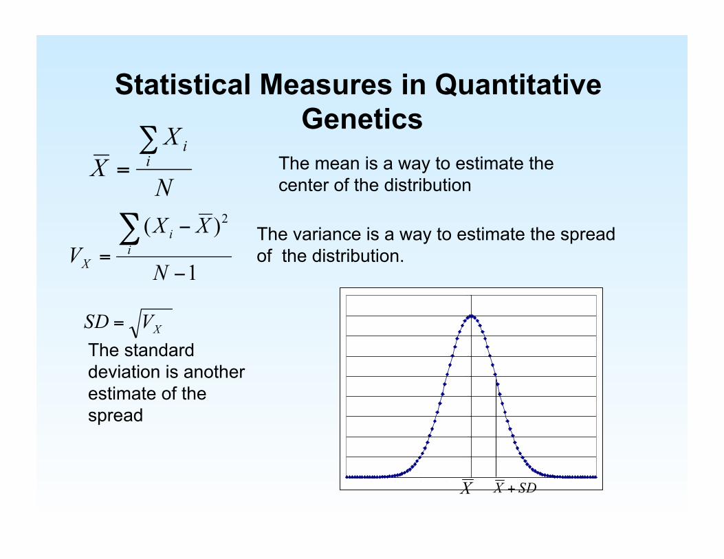
Statistical Measures in Quantitative Genetics

The mean is a way to estimate the center of the distribution

The variance is a way to estimate the spread of the distribution.

The standard deviation is another estimate of the spread

Correlation between X and Y

-4 -3 -2 -1 0 1 2 3 4

-4 -2 0 2 4

j

-4 -3 -2 -1 0 1 2 3 4

-4 -3 -2 -1 0 1 2 3 4

-4 -2 0 2 4

-4 -2 0 2 4

Correlation is an Important Concept in Quantitative Genetics

The covariance is a way to measure the tendency for two variables to have the same location in their distributions.

The correlation is a standardized (measurement scale free) covariance. Perfect + correlation r = 1 No correlation r = 0

Why use Quantitative Traits?

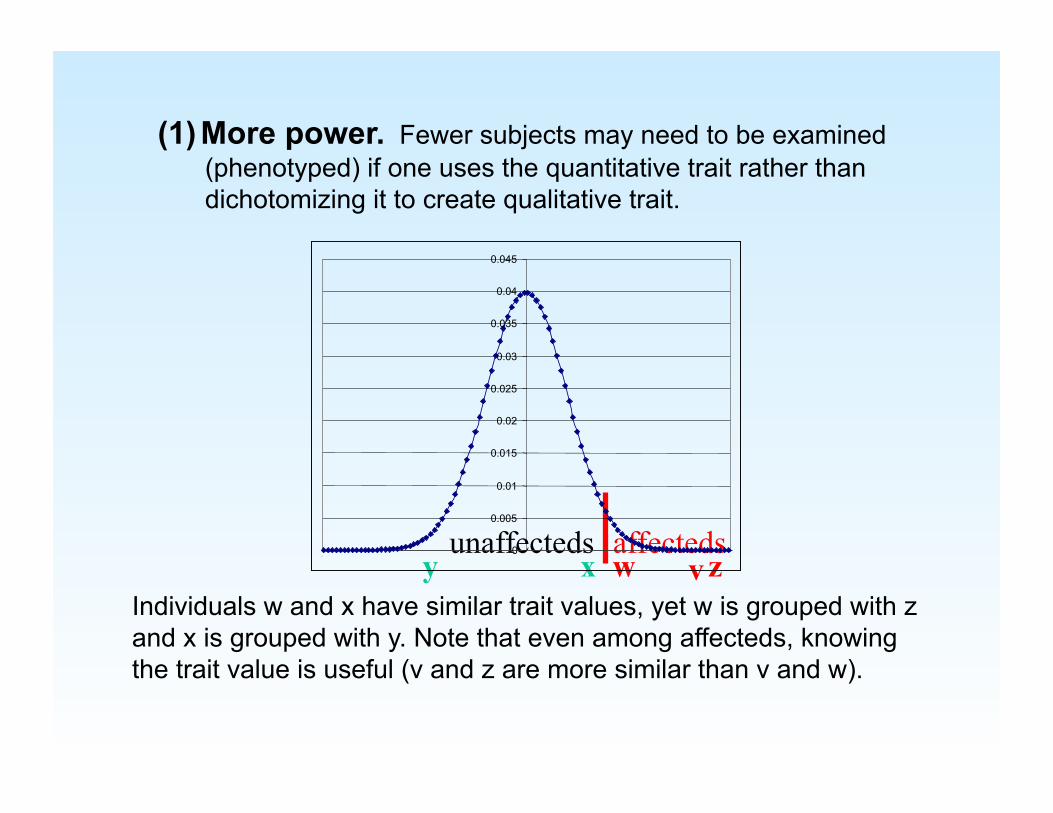
(1) More power. Fewer subjects may need to be examined (phenotyped) if one uses the quantitative trait rather than dichotomizing it to create qualitative trait.

affecteds x y w z

unaffecteds

Individuals w and x have similar trait values, yet w is grouped with z and x is grouped with y. Note that even among affecteds, knowing the trait value is useful (v and z are more similar than v and w).

v 0

0.005 0.01

0.015 0.02

0.025 0.03

0.035 0.04

0.045

-5 5

(2) The genotype to phenotype relationship may be more direct.

Affection with a disease could be the culmination of many underlying events involving gene products, environmental factors and gene-environment interactions. The underlying events may differ among people, resulting in heterogeneity.

When are Quantitative Traits Problematic?

(1)  The quantitative trait doesn’t meet the assumptions of the proposed statistical method. For example many methods assume the quantitative traits are unimodal but not all quantitative traits are unimodal.

(2) The values of the quantitative trait might be very unreliable.

(3) There are no good intermediate quantitative phenotypes for a particular disease. The quantitative traits available aren’t telling the whole story.

0 0.02 0.04 0.06 0.08

0.1

0 50 100 150 200 trait value

freq

uenc

y

A/A

A/G

G/G

=Y

Basic Premise: The Quantitative Trait Values vary with Genotype

A gene that influences a quantitative trait’s value is called a quantitative trait locus (QTL).

The Architecture of the Genotypic Variance

The genotypic variance of the trait can be due to a single major QTL, a few QTLs with large effects (oligogenic) or many QTLs with small effects (polygenic), or combinations of all three.

The individual genes may act on the variance in an additive manner or there may be interaction, or epistatic, relationships between the genes.

How can a few genes and their alleles which are discrete lead to something that looks essentially normally distributed?

Quantitative Traits as the Result of Some Number of Bi-allelic Genes Suppose 3 genes control the trait value. Also suppose that in our population, each gene has two equally frequent alleles. Label the alleles from gene 1 as A and a, the alleles from gene 2 as B and b,and the alleles from gene 3 as C and c. Let A, B, C add one to the phenotype value and let a, b, c subtract one from the phenotype value. So an individual with the A/a B/b C/c genotype has phenotype value = 0 What if the genotype is A/A B/b c/c? or A/A B/B C/C?

Now “genotype” a sample of the population.

Theoretical Phenotype Distribution

Even with only 3 genes, the discrete phenotype is well approximated by a normal distribution. The normal density is bell-like, symmetric, has mean and has inflection points (points where the second derivative is zero) at and . As the number of genes increases, the approximation improves. This scenario is the idea behind a polygenic model.

Population Based Studies of Quantitative Traits

Analysis Conducted with g enotypes

Trait values and genotypes: Let Y denote the trait value. If Y depends on the alleles at locus T, then we expect that knowing the alleles at T would help us predict the value of Y .

0 0.02 0.04 0.06 0.08

0.1

0 50 100 150 200 trait value

freq

uenc

y

A/A

A/G

G/G

=Y

SNP1 QTL

θ

But we don’t Actually Know the Position of the Trait Locus

T/T C/T

C/C

As the distance between the marker locus and the trait locus decreases the marker alleles becomes a good predictor of the trait value.

How can We Test for Association between a SNP and a Quantitative

Trait? Collect phenotype and genotype data

from a number of unrelated individuals. Just like a case-control study but there are no cases and no controls – just individuals with a range of phenotype values.

Hypothetical Data Example

•  Vitamin D receptor gene and women’s height.

•  Measure 128 women between the ages of 30-40.

•  Genotype a SNP in the Vitamin D receptor

Results

Genotype | number Mean SD Min Max -------------+---------------------------------------- 1/1 | 53 63.01 3.71 55.76 71.25 1/2 | 54 64.52 2.86 58.18 71.82 2/2 | 21 66.39 2.95 60.66 70.48

Do the means change with the number of 2 alleles present in the genotype?

Trend (Correlation) Test

•  Test whether r (the correlation) is significantly different from zero.

•  For our example: the calculated value of r is 0.3452. It is significantly different from zero, p-value = 0.0001

•  This trend test is the test used by Cho et al. (2009) in their association analysis

More Generally: QTL Association using Linear Regression

•  Example: height and vitamin D receptor genotypes A/A, A/B, B/B. Let S be the number of B alleles in person i’s genotype

•  Linear regression allows us to include covariates and expand our sample to include males and females effects and other covariates such as age

•  How can we code for an interaction between age and SNP?

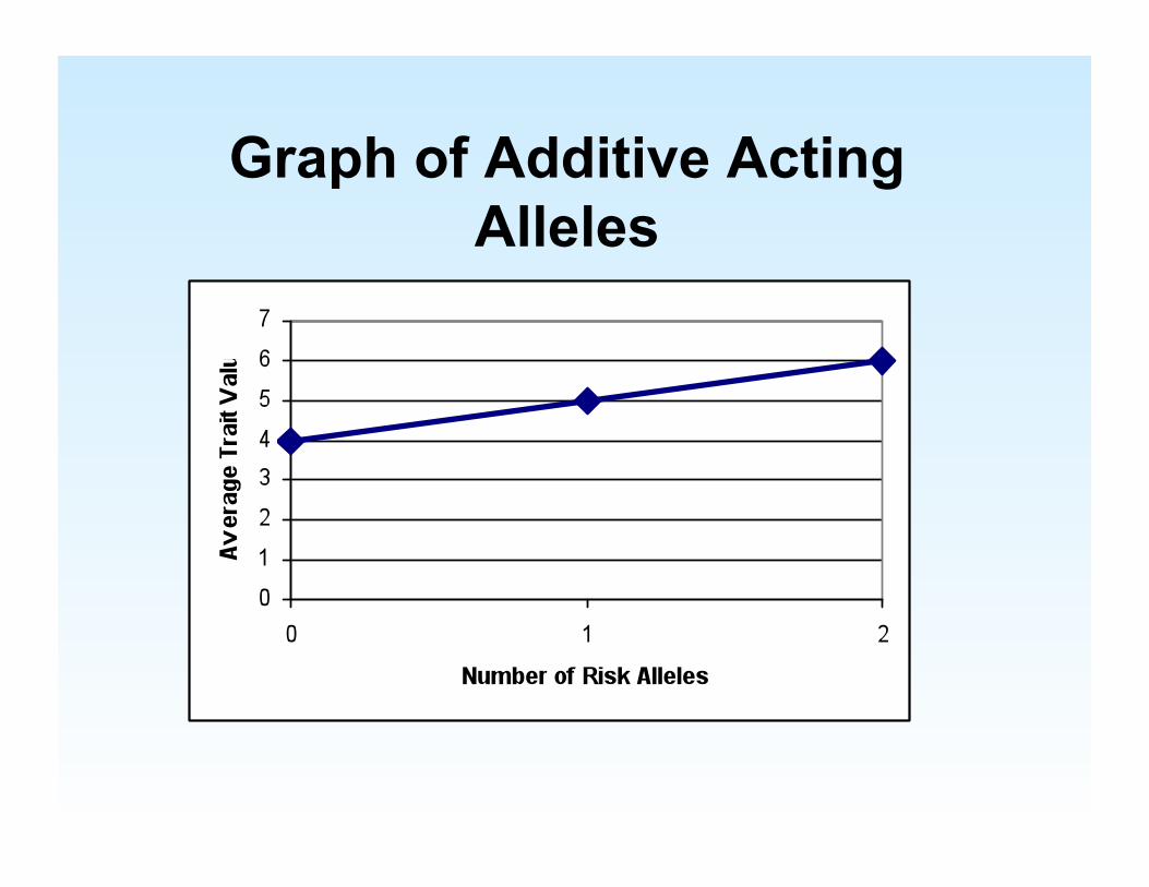
Graph of Additive Acting Alleles

Dominance effect Additive Effect

What if Allele Effects aren’t Additive? Dominance Effects

Cho et al. 2009 GWAS

•  8 Quantitative traits •  ~300K markers

–  Guard against false positives by using an arbitrary stage 1 threshold (P value <10-5 with P value <0.01 in both Ansung and Ansan)

–  Replication of SNPs passing stage 1 in another sample

•  Study Sample: ~4000 individuals from Ansung (rural) ~4000 individuals from Ansan (urban)

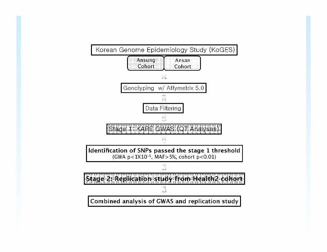
Cho et al. Take Care to Remove Data that Could Lead to Spurious Results

•  Samples with low call rates (<96%), n = 401

•  Samples with evidence of contamination, n =11

•  Samples with sex inconsistencies, n =41 •  Samples with cryptic relatedness, n = 608 •  Samples with serious illnesses, n = 101

Population Stratification can Cause Spurious Results

•  If the sample consists of two or more populations with different allele frequencies and different trait value distributions, one could see evidence of an association.

•  Because they have samples from two regions of Korea, Cho et al. check for evidence of population stratification.

Simple Illustration of Population Stratification for a Qualitative trait (cases/controls).

•  Disease risk is not dependent on SNP allele. –  Within a population allele frequencies for cases and controls are

the same.

•  Odds of disease differs pop 1 versus pop 2. OR = 9 –  1000 cases (800 pop 1, 200 pop 2), 1000 controls (200 pop1,

800 pop 2) •  Allele frequencies differ between cases and controls

–  Prob(allele 1 | pop 1) = .7, Prob(allele 1 | pop 2) = .3 –  Assume HWE holds in both populations.

•  Allele 1 frequency in cases = .8*.7+.2*.3 = .62 •  Allele 1 frequencies in controls = .2*.7+.8*.3 = .38 •  Would lead to a highly significant association result.

Graphical Display – Combined Populations

Pr (case)

Graphical Display for Each Population

Pr (case)

Pop 1

Pr (case)

Pop 2

What if we also have Family Data?

•  Why can’t the linear regression model be applied to family data as is?

•  What could go wrong with this model when we have related individuals?

QTL Association - with a Variance Components Model

Appropriate Study Design

•  Families, unrelated individuals or a mixture can be used, best results with extended pedigrees.

•  Quantitative trait outcomes that can be transformed to normality.

•  Random ascertainment of families or ascertainment through explicitly defined probands are best.

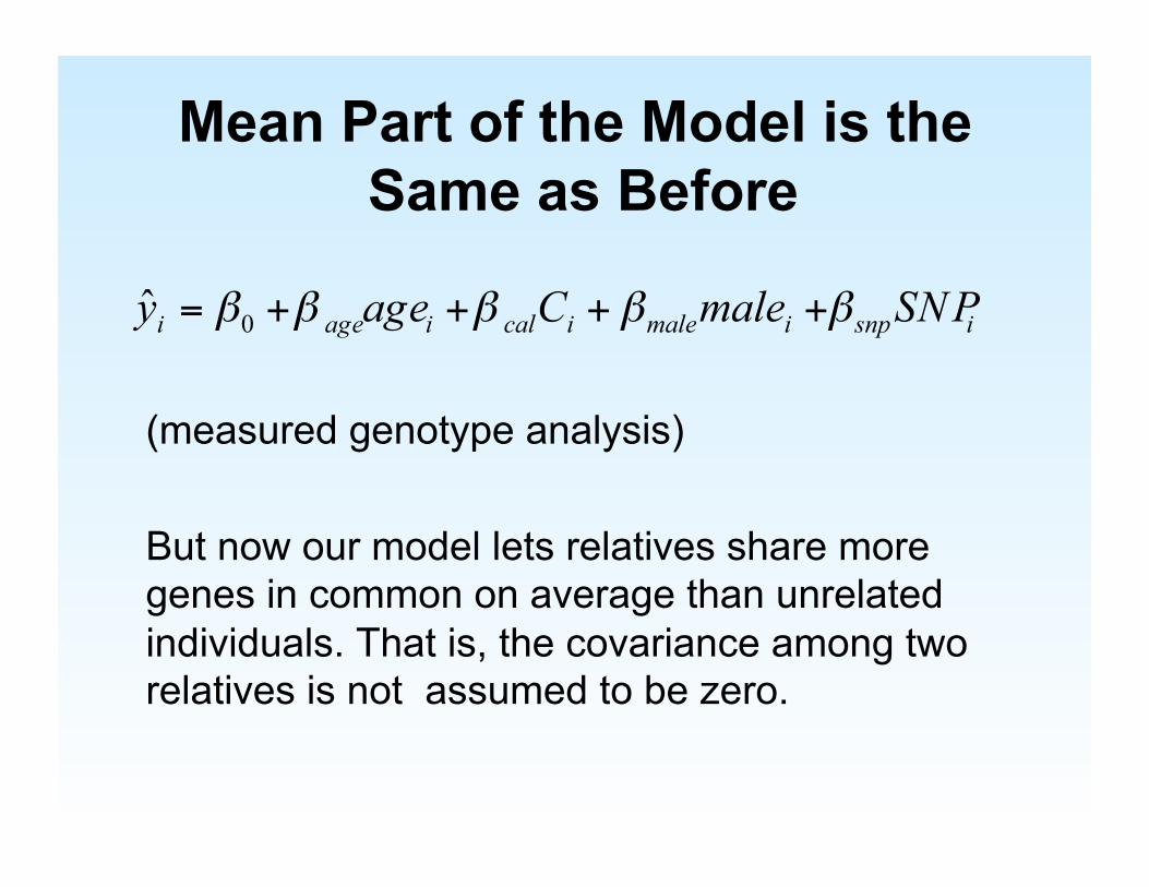
Mean Part of the Model is the Same as Before

(measured genotype analysis)

But now our model lets relatives share more genes in common on average than unrelated individuals. That is, the covariance among two relatives is not assumed to be zero.

Familial Correlation handled through Polygenic Inheritance

•  Polygenic inheritance assumes that the trait is determined by many genes with small additive effects

•  The distribution of the trait values in a population follows a normal distribution, whose location and scale depend on the mean and variance of the trait.

•  The bivariate distributions of relative pairs are 2-dimensional normal distributions – ellipsoidal level curves whose shape depends on the heritability of the trait.

Example: Sibling Correlation for Height

Correlation is not caused by a single gene, caused by many genes and common environment

-4

-2

0

2

4

-4 -2 0 2 4

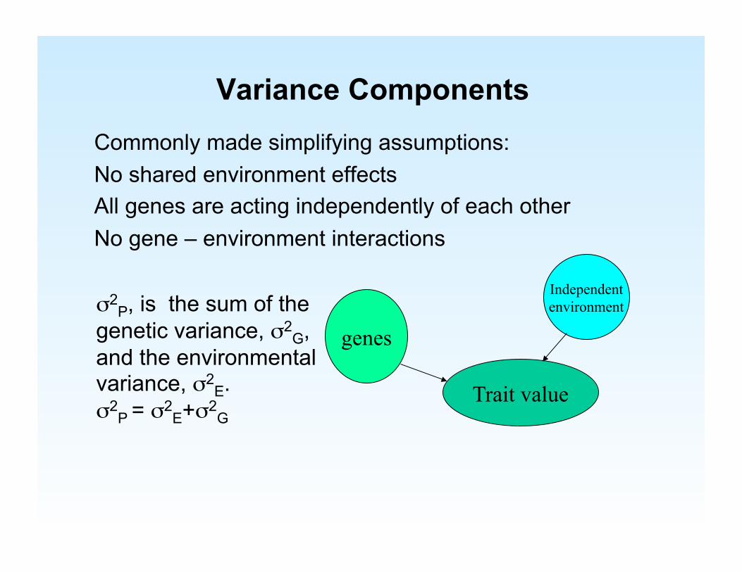
Variance Components Commonly made simplifying assumptions: No shared environment effects All genes are acting independently of each other No gene – environment interactions

genes

Independent environment

Trait value

σ2P, is the sum of the

genetic variance, σ2G,

and the environmental variance, σ2

E. σ2

P = σ2E+σ2

G

The Degree of Correlation between Two Relatives Depends on just how

Closely Related they are •  An important measure of family relationship is the

theoretical kinship coefficient. •  It is the probability that two genes, at a randomly

chosen locus, one chosen randomly from individual i and one from j are identical by descent.

•  The kinship coefficient , Φij , does not depend on the observed genotype data.

•  The theoretical kinship coefficient is not enough to uniquely defend relationships. Φij =1/4 for siblings and for parent-child.

•  Let Δij = the probability that i and j share two genes IBD.

Covariance among Relatives

•  cov(Yi,Yj)=2Φij σ2A+Δij σ2

D •  The more closely related i and j, the

greater the similarity between their trait values is expected to be

•  In our example, we will assume the dominance variance equals zero, then the covariance among relatives i and j is: cov(Yi,Yj)=2Φij σ2

A

Correlation between X and Y

-4 -3 -2 -1 0 1 2 3 4

-4 -2 0 2 4

j

-4 -3 -2 -1 0 1 2 3 4

-4 -3 -2 -1 0 1 2 3 4

-4 -2 0 2 4

-4 -2 0 2 4

Could relatives trait values be this highly correlated?

Population Stratification can Cause Spurious Association in

this Model

•  Need to allow for different allelic effects in different populations.

Data Analysis •  50 two generation nuclear families 236

individuals •  Use a variance component model: Trait levels

as outcome, and sex, bmi, and age as covariates.

•  Account for variation among relatives with an additive polygenic variance term.

•  Compare results with and without a SNP as a covariate.

Model Parameter values

β0 βfemale βbmi βage σ2A σ2

E βsnp Log-likeli-hood

-SNP HO

3.799 .1392 .0092 .003 .0245 .0286 .000 199.63

+SNP HA

3.868 .1252 .0083 .002 .0272 .0255 -.037 203.72

Compare Models using Likelihood Ratio Tests

• Models must be nested to use the LRT. For example the no SNP model is a special case of SNP model • The null hypothesis is the special case model • Alternative hypothesis is the general case model • LRT = 2*(LLgen – LLspec) ~ χ2 distribution, df = mgen - mspec • P-value = probability of getting an LRT as big or bigger when the null hypothesis is true. • If the p-value is less than 0.05 (for example) then reject the null hypothesis (in favor of the alternative hypothesis) • If the p-value is greater than 0.05 then fail to reject the null hypothesis • For our example: LRT =2*(203.72-199.63) = 8.18 • P-value = 0.0042

Family Based Association Methods for Quantitative Traits •  Methods that test whether the apparent

transmission of an allele from parent to offspring depends on the offspring’s phenotype value – Examples: FBAT; Mendel’s Gamete Competition

•  Methods that treat the genotype at the marker as a covariate in a regression analysis, “measured genotype analysis”. –  Examples: Mendel’s QTL Association and

Association given Linkage; QTDT (Abecassis)