analysis of greedy for vertex cover · analysis of greedy for vertex cover 35.1 the vertex-cover...
TRANSCRIPT
Analysis of Greedy for Vertex Cover
35.1 The vertex-cover problem 1109
b c d
a e f g(a)
b c d
a e f g(b)
b c d
a e f g(c)
b c d
a e f g(d)
b c d
a e f g(e)
b c d
a e f g(f)
Figure 35.1 The operation of APPROX-VERTEX-COVER. (a) The input graph G, which has 7vertices and 8 edges. (b) The edge .b; c/, shown heavy, is the first edge chosen by APPROX-VERTEX-COVER. Vertices b and c, shown lightly shaded, are added to the set C containing the vertex coverbeing created. Edges .a; b/, .c; e/, and .c; d/, shown dashed, are removed since they are now coveredby some vertex in C . (c) Edge .e; f / is chosen; vertices e and f are added to C . (d) Edge .d; g/is chosen; vertices d and g are added to C . (e) The set C , which is the vertex cover produced byAPPROX-VERTEX-COVER, contains the six vertices b; c; d; e; f; g. (f) The optimal vertex cover forthis problem contains only three vertices: b, d , and e.
APPROX-VERTEX-COVER.G/
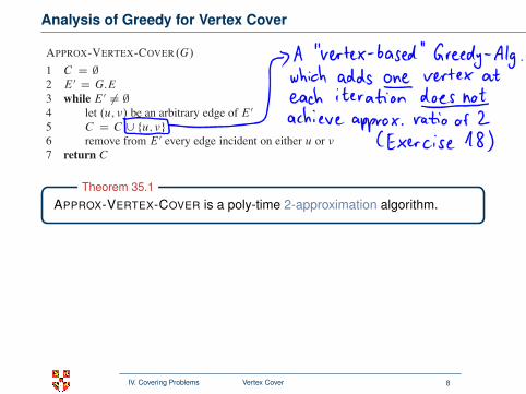
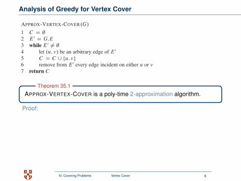
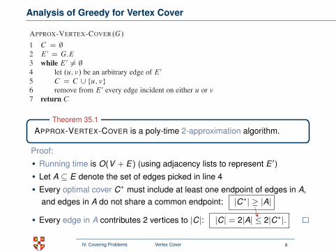
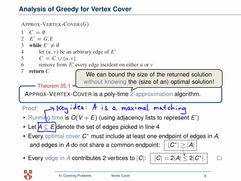
1 C D ;2 E 0 D G:E3 while E 0 ¤ ;4 let .u; !/ be an arbitrary edge of E 0
5 C D C [ fu; !g6 remove from E 0 every edge incident on either u or !7 return C
Figure 35.1 illustrates how APPROX-VERTEX-COVER operates on an examplegraph. The variable C contains the vertex cover being constructed. Line 1 ini-tializes C to the empty set. Line 2 sets E 0 to be a copy of the edge set G:E ofthe graph. The loop of lines 3–6 repeatedly picks an edge .u; !/ from E 0, adds its
APPROX-VERTEX-COVER is a poly-time 2-approximation algorithm.Theorem 35.1
Proof:
Running time is O(V + E) (using adjacency lists to represent E ′)
Let A ⊆ E denote the set of edges picked in line 4
Every optimal cover C∗ must include at least one endpoint of edges in A,
and edges in A do not share a common endpoint: |C∗| ≥ |A|
Every edge in A contributes 2 vertices to |C|:
|C| = 2|A|
≤ 2|C∗|.
We can bound the size of the returned solutionwithout knowing the (size of an) optimal solution!
IV. Covering Problems Vertex Cover 8
Analysis of Greedy for Vertex Cover
35.1 The vertex-cover problem 1109
b c d
a e f g(a)
b c d
a e f g(b)
b c d
a e f g(c)
b c d
a e f g(d)
b c d
a e f g(e)
b c d
a e f g(f)
Figure 35.1 The operation of APPROX-VERTEX-COVER. (a) The input graph G, which has 7vertices and 8 edges. (b) The edge .b; c/, shown heavy, is the first edge chosen by APPROX-VERTEX-COVER. Vertices b and c, shown lightly shaded, are added to the set C containing the vertex coverbeing created. Edges .a; b/, .c; e/, and .c; d/, shown dashed, are removed since they are now coveredby some vertex in C . (c) Edge .e; f / is chosen; vertices e and f are added to C . (d) Edge .d; g/is chosen; vertices d and g are added to C . (e) The set C , which is the vertex cover produced byAPPROX-VERTEX-COVER, contains the six vertices b; c; d; e; f; g. (f) The optimal vertex cover forthis problem contains only three vertices: b, d , and e.
APPROX-VERTEX-COVER.G/
1 C D ;2 E 0 D G:E3 while E 0 ¤ ;4 let .u; !/ be an arbitrary edge of E 0
5 C D C [ fu; !g6 remove from E 0 every edge incident on either u or !7 return C
Figure 35.1 illustrates how APPROX-VERTEX-COVER operates on an examplegraph. The variable C contains the vertex cover being constructed. Line 1 ini-tializes C to the empty set. Line 2 sets E 0 to be a copy of the edge set G:E ofthe graph. The loop of lines 3–6 repeatedly picks an edge .u; !/ from E 0, adds its
APPROX-VERTEX-COVER is a poly-time 2-approximation algorithm.Theorem 35.1
Proof:
Running time is O(V + E) (using adjacency lists to represent E ′)
Let A ⊆ E denote the set of edges picked in line 4
Every optimal cover C∗ must include at least one endpoint of edges in A,and edges in A do not share a common endpoint: |C∗| ≥ |A|
Every edge in A contributes 2 vertices to |C|: |C| = 2|A| ≤ 2|C∗|.
We can bound the size of the returned solutionwithout knowing the (size of an) optimal solution!
IV. Covering Problems Vertex Cover 8
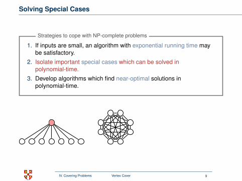
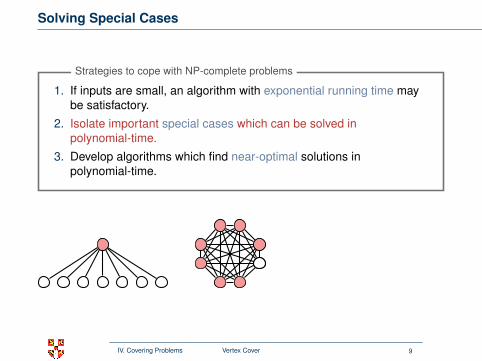
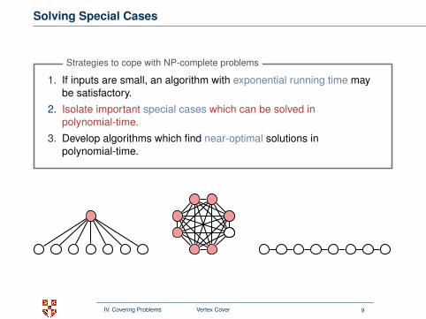
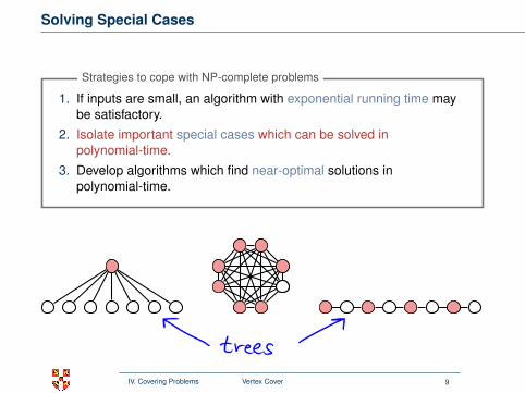
Solving Special Cases
1. If inputs are small, an algorithm with exponential running time maybe satisfactory.
2. Isolate important special cases which can be solved inpolynomial-time.
3. Develop algorithms which find near-optimal solutions inpolynomial-time.
Strategies to cope with NP-complete problems
IV. Covering Problems Vertex Cover 9
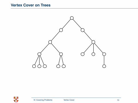
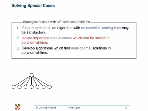
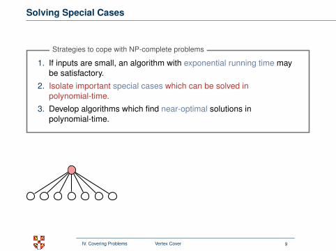
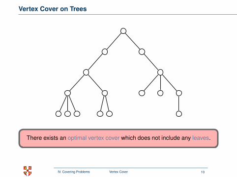
Vertex Cover on Trees
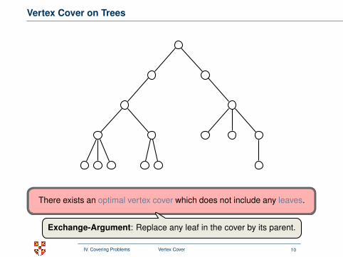
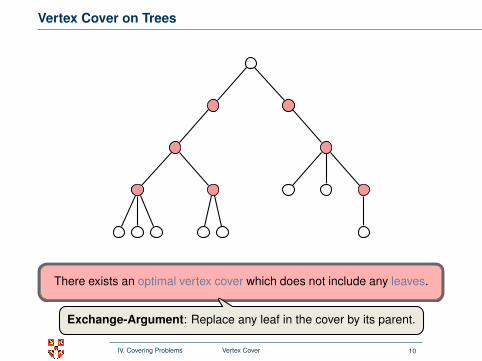
There exists an optimal vertex cover which does not include any leaves.
Exchange-Argument: Replace any leaf in the cover by its parent.
IV. Covering Problems Vertex Cover 10
Vertex Cover on Trees
There exists an optimal vertex cover which does not include any leaves.
Exchange-Argument: Replace any leaf in the cover by its parent.
IV. Covering Problems Vertex Cover 10
Vertex Cover on Trees
There exists an optimal vertex cover which does not include any leaves.
Exchange-Argument: Replace any leaf in the cover by its parent.
IV. Covering Problems Vertex Cover 10

Vertex Cover on Trees
There exists an optimal vertex cover which does not include any leaves.
Exchange-Argument: Replace any leaf in the cover by its parent.
IV. Covering Problems Vertex Cover 10

Vertex Cover on Trees
There exists an optimal vertex cover which does not include any leaves.
Exchange-Argument: Replace any leaf in the cover by its parent.
IV. Covering Problems Vertex Cover 10
Vertex Cover on Trees
There exists an optimal vertex cover which does not include any leaves.
Exchange-Argument: Replace any leaf in the cover by its parent.
IV. Covering Problems Vertex Cover 10
Solving Vertex Cover on Trees
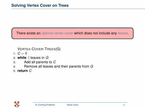
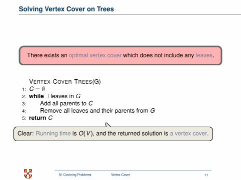
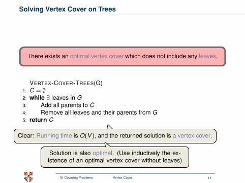
There exists an optimal vertex cover which does not include any leaves.
VERTEX-COVER-TREES(G)1: C = ∅2: while ∃ leaves in G3: Add all parents to C4: Remove all leaves and their parents from G5: return C
Clear: Running time is O(V ), and the returned solution is a vertex cover.
Solution is also optimal. (Use inductively the ex-istence of an optimal vertex cover without leaves)
IV. Covering Problems Vertex Cover 11
Solving Vertex Cover on Trees
There exists an optimal vertex cover which does not include any leaves.
VERTEX-COVER-TREES(G)1: C = ∅2: while ∃ leaves in G3: Add all parents to C4: Remove all leaves and their parents from G5: return C
Clear: Running time is O(V ), and the returned solution is a vertex cover.
Solution is also optimal. (Use inductively the ex-istence of an optimal vertex cover without leaves)
IV. Covering Problems Vertex Cover 11
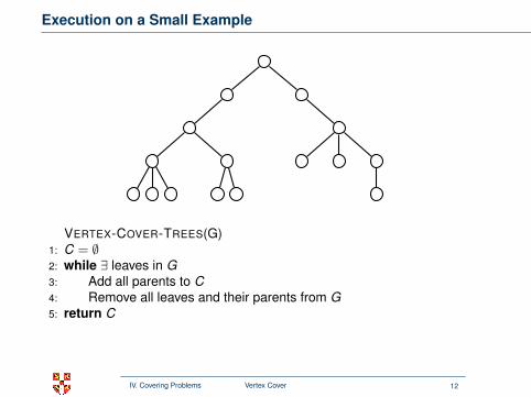
Execution on a Small Example
After iteration
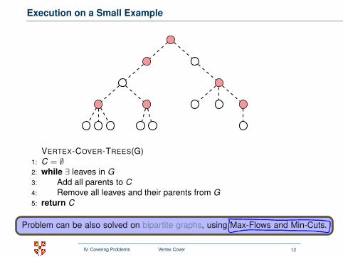
VERTEX-COVER-TREES(G)1: C = ∅2: while ∃ leaves in G3: Add all parents to C4: Remove all leaves and their parents from G5: return C
Problem can be also solved on bipartite graphs, using Max-Flows and Min-Cuts.
IV. Covering Problems Vertex Cover 12
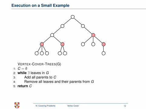
Execution on a Small Example
After iteration
VERTEX-COVER-TREES(G)1: C = ∅2: while ∃ leaves in G3: Add all parents to C4: Remove all leaves and their parents from G5: return C
Problem can be also solved on bipartite graphs, using Max-Flows and Min-Cuts.
IV. Covering Problems Vertex Cover 12
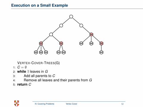
Execution on a Small Example
After iteration
VERTEX-COVER-TREES(G)1: C = ∅2: while ∃ leaves in G3: Add all parents to C4: Remove all leaves and their parents from G5: return C
Problem can be also solved on bipartite graphs, using Max-Flows and Min-Cuts.
IV. Covering Problems Vertex Cover 12

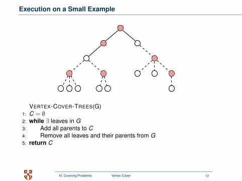
Execution on a Small Example
After iteration
VERTEX-COVER-TREES(G)1: C = ∅2: while ∃ leaves in G3: Add all parents to C4: Remove all leaves and their parents from G5: return C
Problem can be also solved on bipartite graphs, using Max-Flows and Min-Cuts.
IV. Covering Problems Vertex Cover 12
Execution on a Small Example
After iteration
VERTEX-COVER-TREES(G)1: C = ∅2: while ∃ leaves in G3: Add all parents to C4: Remove all leaves and their parents from G5: return C
Problem can be also solved on bipartite graphs, using Max-Flows and Min-Cuts.
IV. Covering Problems Vertex Cover 12

Execution on a Small Example
After iteration
VERTEX-COVER-TREES(G)1: C = ∅2: while ∃ leaves in G3: Add all parents to C4: Remove all leaves and their parents from G5: return C
Problem can be also solved on bipartite graphs, using Max-Flows and Min-Cuts.
IV. Covering Problems Vertex Cover 12

Execution on a Small Example
After iteration
VERTEX-COVER-TREES(G)1: C = ∅2: while ∃ leaves in G3: Add all parents to C4: Remove all leaves and their parents from G5: return C
Problem can be also solved on bipartite graphs, using Max-Flows and Min-Cuts.
IV. Covering Problems Vertex Cover 12
Execution on a Small Example
After iteration
VERTEX-COVER-TREES(G)1: C = ∅2: while ∃ leaves in G3: Add all parents to C4: Remove all leaves and their parents from G5: return C
Problem can be also solved on bipartite graphs, using Max-Flows and Min-Cuts.
IV. Covering Problems Vertex Cover 12
Exact Algorithms
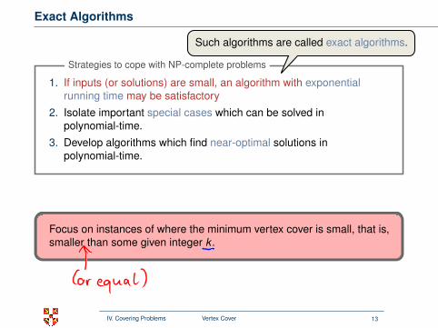
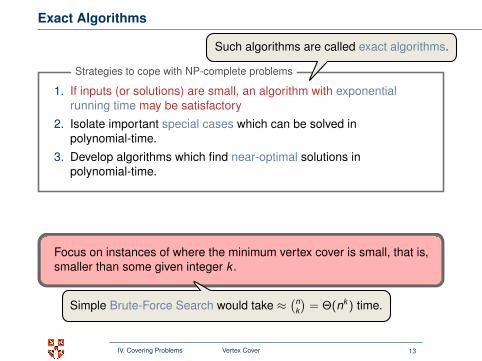
1. If inputs (or solutions) are small, an algorithm with exponentialrunning time may be satisfactory
2. Isolate important special cases which can be solved inpolynomial-time.
3. Develop algorithms which find near-optimal solutions inpolynomial-time.
Strategies to cope with NP-complete problems
Such algorithms are called exact algorithms.
Focus on instances of where the minimum vertex cover is small, that is,smaller than some given integer k .
Simple Brute-Force Search would take ≈(n
k
)= Θ(nk ) time.
IV. Covering Problems Vertex Cover 13
Exact Algorithms
1. If inputs (or solutions) are small, an algorithm with exponentialrunning time may be satisfactory
2. Isolate important special cases which can be solved inpolynomial-time.
3. Develop algorithms which find near-optimal solutions inpolynomial-time.
Strategies to cope with NP-complete problems
Such algorithms are called exact algorithms.
Focus on instances of where the minimum vertex cover is small, that is,smaller than some given integer k .
Simple Brute-Force Search would take ≈(n
k
)= Θ(nk ) time.
IV. Covering Problems Vertex Cover 13
Towards a more efficient Search
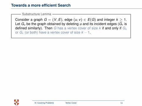
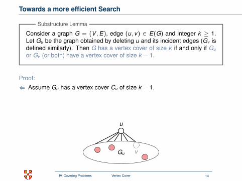
Consider a graph G = (V ,E), edge (u, v) ∈ E(G) and integer k ≥ 1.Let Gu be the graph obtained by deleting u and its incident edges (Gv isdefined similarly). Then G has a vertex cover of size k if and only if Gu
or Gv (or both) have a vertex cover of size k − 1.
Substructure Lemma
Reminiscent of Dynamic Programming.Proof:
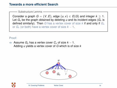
⇐ Assume Gu has a vertex cover Cu of size k − 1.
Adding u yields a vertex cover of G which is of size k
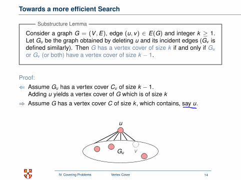
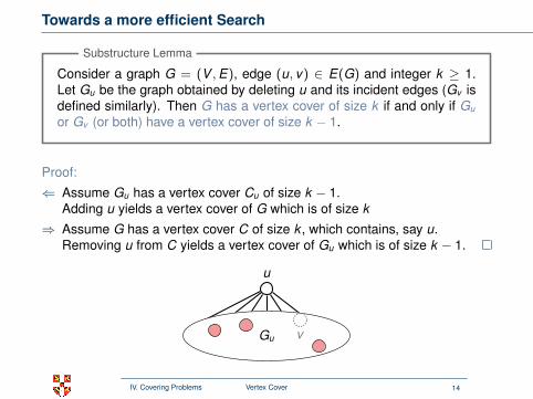
⇒ Assume G has a vertex cover C of size k , which contains, say u.
Removing u from C yields a vertex cover of Gu which is of size k − 1.
uu
Gu v
IV. Covering Problems Vertex Cover 14
Towards a more efficient Search
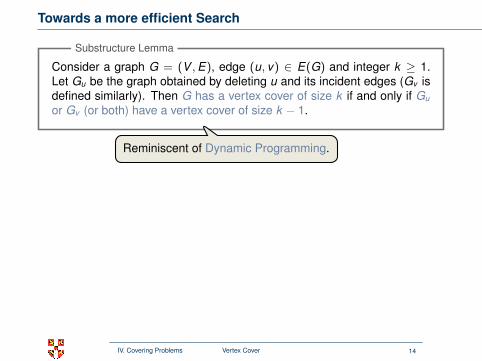
Consider a graph G = (V ,E), edge (u, v) ∈ E(G) and integer k ≥ 1.Let Gu be the graph obtained by deleting u and its incident edges (Gv isdefined similarly). Then G has a vertex cover of size k if and only if Gu
or Gv (or both) have a vertex cover of size k − 1.
Substructure Lemma
Reminiscent of Dynamic Programming.
Proof:
⇐ Assume Gu has a vertex cover Cu of size k − 1.
Adding u yields a vertex cover of G which is of size k
⇒ Assume G has a vertex cover C of size k , which contains, say u.
Removing u from C yields a vertex cover of Gu which is of size k − 1.
uu
Gu v
IV. Covering Problems Vertex Cover 14
Towards a more efficient Search
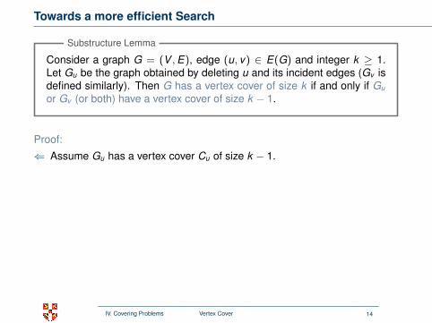
Consider a graph G = (V ,E), edge (u, v) ∈ E(G) and integer k ≥ 1.Let Gu be the graph obtained by deleting u and its incident edges (Gv isdefined similarly). Then G has a vertex cover of size k if and only if Gu
or Gv (or both) have a vertex cover of size k − 1.
Substructure Lemma
Reminiscent of Dynamic Programming.
Proof:
⇐ Assume Gu has a vertex cover Cu of size k − 1.
Adding u yields a vertex cover of G which is of size k
⇒ Assume G has a vertex cover C of size k , which contains, say u.
Removing u from C yields a vertex cover of Gu which is of size k − 1.
uu
Gu v
IV. Covering Problems Vertex Cover 14
Towards a more efficient Search
Consider a graph G = (V ,E), edge (u, v) ∈ E(G) and integer k ≥ 1.Let Gu be the graph obtained by deleting u and its incident edges (Gv isdefined similarly). Then G has a vertex cover of size k if and only if Gu
or Gv (or both) have a vertex cover of size k − 1.
Substructure Lemma
Reminiscent of Dynamic Programming.
Proof:
⇐ Assume Gu has a vertex cover Cu of size k − 1.
Adding u yields a vertex cover of G which is of size k
⇒ Assume G has a vertex cover C of size k , which contains, say u.
Removing u from C yields a vertex cover of Gu which is of size k − 1.
u
u
Gu v
IV. Covering Problems Vertex Cover 14
Towards a more efficient Search
Consider a graph G = (V ,E), edge (u, v) ∈ E(G) and integer k ≥ 1.Let Gu be the graph obtained by deleting u and its incident edges (Gv isdefined similarly). Then G has a vertex cover of size k if and only if Gu
or Gv (or both) have a vertex cover of size k − 1.
Substructure Lemma
Reminiscent of Dynamic Programming.
Proof:
⇐ Assume Gu has a vertex cover Cu of size k − 1.Adding u yields a vertex cover of G which is of size k
⇒ Assume G has a vertex cover C of size k , which contains, say u.Removing u from C yields a vertex cover of Gu which is of size k − 1.
u
u
Gu v
IV. Covering Problems Vertex Cover 14
A More Efficient Search Algorithm
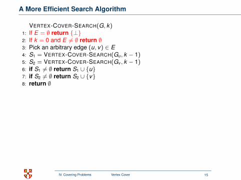
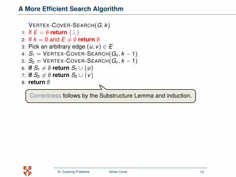
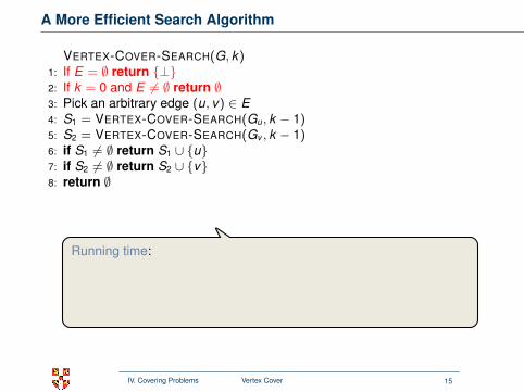
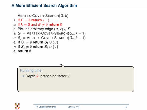
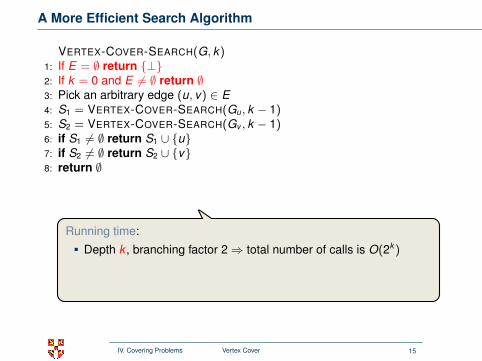
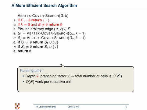
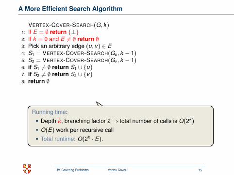
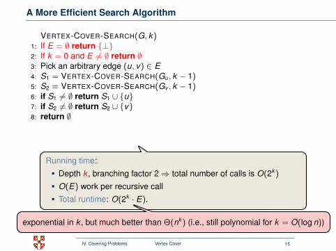
VERTEX-COVER-SEARCH(G, k)1: If E = ∅ return {⊥}2: If k = 0 and E 6= ∅ return ∅3: Pick an arbitrary edge (u, v) ∈ E4: S1 = VERTEX-COVER-SEARCH(Gu, k − 1)5: S2 = VERTEX-COVER-SEARCH(Gv , k − 1)6: if S1 6= ∅ return S1 ∪ {u}7: if S2 6= ∅ return S2 ∪ {v}8: return ∅
Correctness follows by the Substructure Lemma and induction.
Running time:
Depth k , branching factor 2
⇒ total number of calls is O(2k )
O(E) work per recursive call
Total runtime: O(2k · E).
exponential in k , but much better than Θ(nk ) (i.e., still polynomial for k = O(log n))
IV. Covering Problems Vertex Cover 15
A More Efficient Search Algorithm
VERTEX-COVER-SEARCH(G, k)1: If E = ∅ return {⊥}2: If k = 0 and E 6= ∅ return ∅3: Pick an arbitrary edge (u, v) ∈ E4: S1 = VERTEX-COVER-SEARCH(Gu, k − 1)5: S2 = VERTEX-COVER-SEARCH(Gv , k − 1)6: if S1 6= ∅ return S1 ∪ {u}7: if S2 6= ∅ return S2 ∪ {v}8: return ∅
Correctness follows by the Substructure Lemma and induction.
Running time:
Depth k , branching factor 2⇒ total number of calls is O(2k )
O(E) work per recursive call
Total runtime: O(2k · E).
exponential in k , but much better than Θ(nk ) (i.e., still polynomial for k = O(log n))
IV. Covering Problems Vertex Cover 15
Outline
Introduction
Vertex Cover
The Set-Covering Problem
IV. Covering Problems The Set-Covering Problem 16
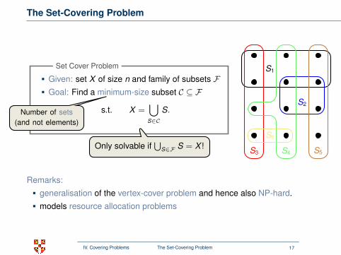
The Set-Covering Problem
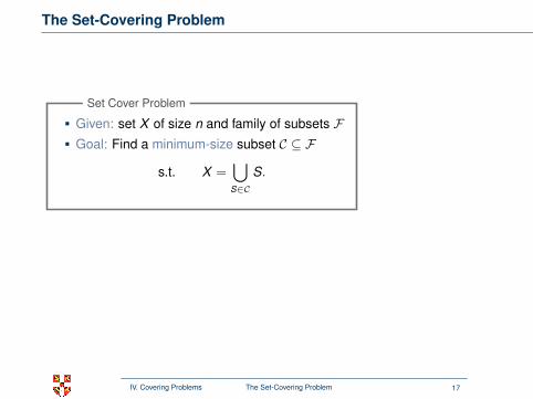
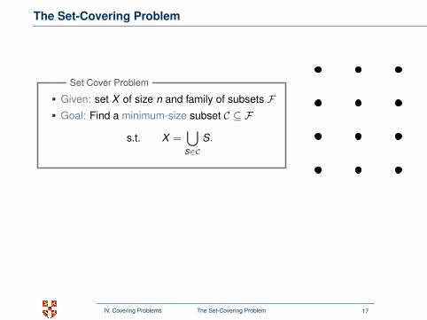
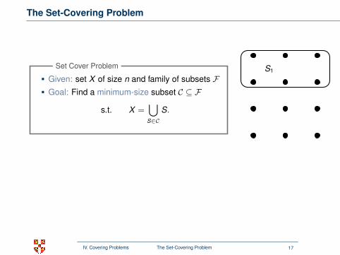
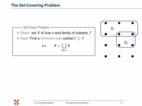
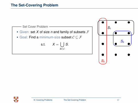
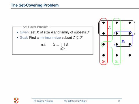
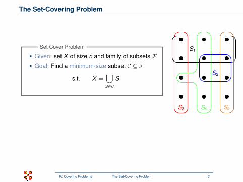
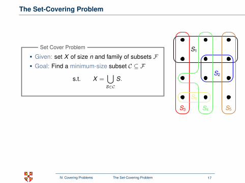
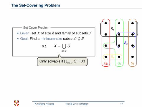
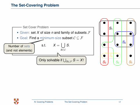
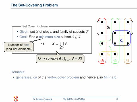
Given: set X of size n and family of subsets FGoal: Find a minimum-size subset C ⊆ F
s.t. X =⋃
S∈C
S.
Set Cover Problem
Only solvable if⋃
S∈F S = X !
Number of sets(and not elements)
S1
S2
S3 S4 S5
S6
Remarks:
generalisation of the vertex-cover problem and hence also NP-hard.
models resource allocation problems
IV. Covering Problems The Set-Covering Problem 17
The Set-Covering Problem
Given: set X of size n and family of subsets FGoal: Find a minimum-size subset C ⊆ F
s.t. X =⋃
S∈C
S.
Set Cover Problem
Only solvable if⋃
S∈F S = X !
Number of sets(and not elements)
S1
S2
S3
S4 S5
S6
Remarks:
generalisation of the vertex-cover problem and hence also NP-hard.
models resource allocation problems
IV. Covering Problems The Set-Covering Problem 17
The Set-Covering Problem
Given: set X of size n and family of subsets FGoal: Find a minimum-size subset C ⊆ F
s.t. X =⋃
S∈C
S.
Set Cover Problem
Only solvable if⋃
S∈F S = X !
Number of sets(and not elements)
S1
S2
S3 S4
S5
S6
Remarks:
generalisation of the vertex-cover problem and hence also NP-hard.
models resource allocation problems
IV. Covering Problems The Set-Covering Problem 17
The Set-Covering Problem
Given: set X of size n and family of subsets FGoal: Find a minimum-size subset C ⊆ F
s.t. X =⋃
S∈C
S.
Set Cover Problem
Only solvable if⋃
S∈F S = X !
Number of sets(and not elements)
S1
S2
S3 S4 S5
S6
Remarks:
generalisation of the vertex-cover problem and hence also NP-hard.
models resource allocation problems
IV. Covering Problems The Set-Covering Problem 17
The Set-Covering Problem
Given: set X of size n and family of subsets FGoal: Find a minimum-size subset C ⊆ F
s.t. X =⋃
S∈C
S.
Set Cover Problem
Only solvable if⋃
S∈F S = X !
Number of sets(and not elements)
S1
S2
S3 S4 S5
S6
Remarks:
generalisation of the vertex-cover problem and hence also NP-hard.
models resource allocation problems
IV. Covering Problems The Set-Covering Problem 17
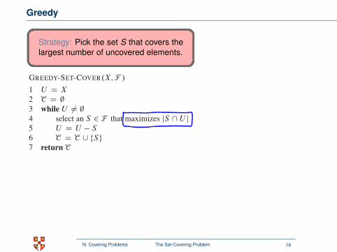
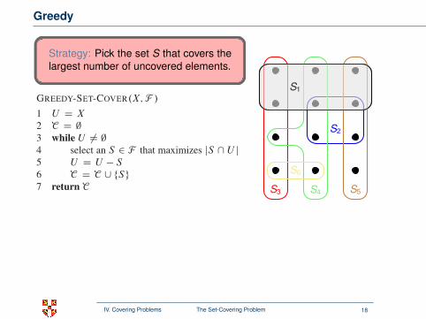
Greedy
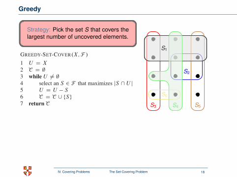
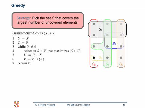
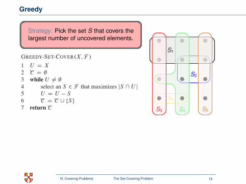
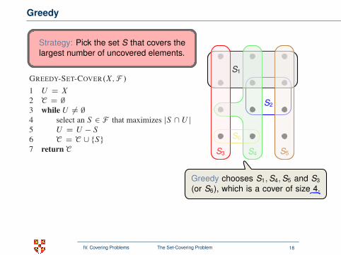
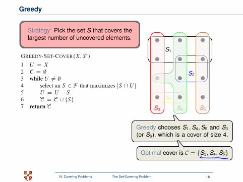
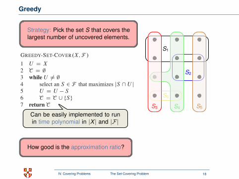
Strategy: Pick the set S that covers thelargest number of uncovered elements.
35.3 The set-covering problem 1119
A greedy approximation algorithmThe greedy method works by picking, at each stage, the set S that covers the great-est number of remaining elements that are uncovered.GREEDY-SET-COVER.X; F /
1 U D X2 C D ;3 while U ¤ ;4 select an S 2 F that maximizes jS \ U j5 U D U ! S6 C D C [ fSg7 return C
In the example of Figure 35.3, GREEDY-SET-COVER adds to C , in order, the setsS1, S4, and S5, followed by either S3 or S6.
The algorithm works as follows. The set U contains, at each stage, the set ofremaining uncovered elements. The set C contains the cover being constructed.Line 4 is the greedy decision-making step, choosing a subset S that covers as manyuncovered elements as possible (breaking ties arbitrarily). After S is selected,line 5 removes its elements from U , and line 6 places S into C . When the algorithmterminates, the set C contains a subfamily of F that covers X .
We can easily implement GREEDY-SET-COVER to run in time polynomial in jX jand jF j. Since the number of iterations of the loop on lines 3–6 is bounded fromabove by min.jX j ; jF j/, and we can implement the loop body to run in timeO.jX j jF j/, a simple implementation runs in time O.jX j jF jmin.jX j ; jF j//. Ex-ercise 35.3-3 asks for a linear-time algorithm.
AnalysisWe now show that the greedy algorithm returns a set cover that is not too muchlarger than an optimal set cover. For convenience, in this chapter we denote the d thharmonic number Hd D
PdiD1 1=i (see Section A.1) by H.d/. As a boundary
condition, we define H.0/ D 0.
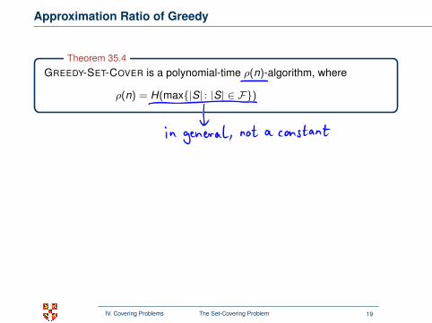
Theorem 35.4GREEDY-SET-COVER is a polynomial-time !.n/-approximation algorithm, where!.n/ D H.max fjS j W S 2 F g/ :
Proof We have already shown that GREEDY-SET-COVER runs in polynomialtime.
Can be easily implemented to runin time polynomial in |X | and |F|
How good is the approximation ratio?
S1
S2
S3 S4 S5
S6
S1
S4 S5S3
Greedy chooses S1,S4,S5 and S3
(or S6), which is a cover of size 4.
Optimal cover is C = {S3,S4,S5}
Optimal cover is C = {S3,S4,S5}
IV. Covering Problems The Set-Covering Problem 18
Greedy
Strategy: Pick the set S that covers thelargest number of uncovered elements.
35.3 The set-covering problem 1119
A greedy approximation algorithmThe greedy method works by picking, at each stage, the set S that covers the great-est number of remaining elements that are uncovered.GREEDY-SET-COVER.X; F /
1 U D X2 C D ;3 while U ¤ ;4 select an S 2 F that maximizes jS \ U j5 U D U ! S6 C D C [ fSg7 return C
In the example of Figure 35.3, GREEDY-SET-COVER adds to C , in order, the setsS1, S4, and S5, followed by either S3 or S6.
The algorithm works as follows. The set U contains, at each stage, the set ofremaining uncovered elements. The set C contains the cover being constructed.Line 4 is the greedy decision-making step, choosing a subset S that covers as manyuncovered elements as possible (breaking ties arbitrarily). After S is selected,line 5 removes its elements from U , and line 6 places S into C . When the algorithmterminates, the set C contains a subfamily of F that covers X .
We can easily implement GREEDY-SET-COVER to run in time polynomial in jX jand jF j. Since the number of iterations of the loop on lines 3–6 is bounded fromabove by min.jX j ; jF j/, and we can implement the loop body to run in timeO.jX j jF j/, a simple implementation runs in time O.jX j jF jmin.jX j ; jF j//. Ex-ercise 35.3-3 asks for a linear-time algorithm.
AnalysisWe now show that the greedy algorithm returns a set cover that is not too muchlarger than an optimal set cover. For convenience, in this chapter we denote the d thharmonic number Hd D
PdiD1 1=i (see Section A.1) by H.d/. As a boundary
condition, we define H.0/ D 0.
Theorem 35.4GREEDY-SET-COVER is a polynomial-time !.n/-approximation algorithm, where!.n/ D H.max fjS j W S 2 F g/ :
Proof We have already shown that GREEDY-SET-COVER runs in polynomialtime.
Can be easily implemented to runin time polynomial in |X | and |F|
How good is the approximation ratio?
S1
S2
S3 S4 S5
S6
S1
S4 S5S3
Greedy chooses S1,S4,S5 and S3
(or S6), which is a cover of size 4.
Optimal cover is C = {S3,S4,S5}
Optimal cover is C = {S3,S4,S5}
IV. Covering Problems The Set-Covering Problem 18
Greedy
Strategy: Pick the set S that covers thelargest number of uncovered elements.
35.3 The set-covering problem 1119
A greedy approximation algorithmThe greedy method works by picking, at each stage, the set S that covers the great-est number of remaining elements that are uncovered.GREEDY-SET-COVER.X; F /
1 U D X2 C D ;3 while U ¤ ;4 select an S 2 F that maximizes jS \ U j5 U D U ! S6 C D C [ fSg7 return C
In the example of Figure 35.3, GREEDY-SET-COVER adds to C , in order, the setsS1, S4, and S5, followed by either S3 or S6.
The algorithm works as follows. The set U contains, at each stage, the set ofremaining uncovered elements. The set C contains the cover being constructed.Line 4 is the greedy decision-making step, choosing a subset S that covers as manyuncovered elements as possible (breaking ties arbitrarily). After S is selected,line 5 removes its elements from U , and line 6 places S into C . When the algorithmterminates, the set C contains a subfamily of F that covers X .
We can easily implement GREEDY-SET-COVER to run in time polynomial in jX jand jF j. Since the number of iterations of the loop on lines 3–6 is bounded fromabove by min.jX j ; jF j/, and we can implement the loop body to run in timeO.jX j jF j/, a simple implementation runs in time O.jX j jF jmin.jX j ; jF j//. Ex-ercise 35.3-3 asks for a linear-time algorithm.
AnalysisWe now show that the greedy algorithm returns a set cover that is not too muchlarger than an optimal set cover. For convenience, in this chapter we denote the d thharmonic number Hd D
PdiD1 1=i (see Section A.1) by H.d/. As a boundary
condition, we define H.0/ D 0.
Theorem 35.4GREEDY-SET-COVER is a polynomial-time !.n/-approximation algorithm, where!.n/ D H.max fjS j W S 2 F g/ :
Proof We have already shown that GREEDY-SET-COVER runs in polynomialtime.
Can be easily implemented to runin time polynomial in |X | and |F|
How good is the approximation ratio?
S1
S2
S3 S4 S5
S6
S1
S4
S5S3
Greedy chooses S1,S4,S5 and S3
(or S6), which is a cover of size 4.
Optimal cover is C = {S3,S4,S5}
Optimal cover is C = {S3,S4,S5}
IV. Covering Problems The Set-Covering Problem 18
Greedy
Strategy: Pick the set S that covers thelargest number of uncovered elements.
35.3 The set-covering problem 1119
A greedy approximation algorithmThe greedy method works by picking, at each stage, the set S that covers the great-est number of remaining elements that are uncovered.GREEDY-SET-COVER.X; F /
1 U D X2 C D ;3 while U ¤ ;4 select an S 2 F that maximizes jS \ U j5 U D U ! S6 C D C [ fSg7 return C
In the example of Figure 35.3, GREEDY-SET-COVER adds to C , in order, the setsS1, S4, and S5, followed by either S3 or S6.
The algorithm works as follows. The set U contains, at each stage, the set ofremaining uncovered elements. The set C contains the cover being constructed.Line 4 is the greedy decision-making step, choosing a subset S that covers as manyuncovered elements as possible (breaking ties arbitrarily). After S is selected,line 5 removes its elements from U , and line 6 places S into C . When the algorithmterminates, the set C contains a subfamily of F that covers X .
We can easily implement GREEDY-SET-COVER to run in time polynomial in jX jand jF j. Since the number of iterations of the loop on lines 3–6 is bounded fromabove by min.jX j ; jF j/, and we can implement the loop body to run in timeO.jX j jF j/, a simple implementation runs in time O.jX j jF jmin.jX j ; jF j//. Ex-ercise 35.3-3 asks for a linear-time algorithm.
AnalysisWe now show that the greedy algorithm returns a set cover that is not too muchlarger than an optimal set cover. For convenience, in this chapter we denote the d thharmonic number Hd D
PdiD1 1=i (see Section A.1) by H.d/. As a boundary
condition, we define H.0/ D 0.
Theorem 35.4GREEDY-SET-COVER is a polynomial-time !.n/-approximation algorithm, where!.n/ D H.max fjS j W S 2 F g/ :
Proof We have already shown that GREEDY-SET-COVER runs in polynomialtime.
Can be easily implemented to runin time polynomial in |X | and |F|
How good is the approximation ratio?
S1
S2
S3 S4 S5
S6
S1
S4 S5
S3
Greedy chooses S1,S4,S5 and S3
(or S6), which is a cover of size 4.
Optimal cover is C = {S3,S4,S5}
Optimal cover is C = {S3,S4,S5}
IV. Covering Problems The Set-Covering Problem 18
Greedy
Strategy: Pick the set S that covers thelargest number of uncovered elements.
35.3 The set-covering problem 1119
A greedy approximation algorithmThe greedy method works by picking, at each stage, the set S that covers the great-est number of remaining elements that are uncovered.GREEDY-SET-COVER.X; F /
1 U D X2 C D ;3 while U ¤ ;4 select an S 2 F that maximizes jS \ U j5 U D U ! S6 C D C [ fSg7 return C
In the example of Figure 35.3, GREEDY-SET-COVER adds to C , in order, the setsS1, S4, and S5, followed by either S3 or S6.
The algorithm works as follows. The set U contains, at each stage, the set ofremaining uncovered elements. The set C contains the cover being constructed.Line 4 is the greedy decision-making step, choosing a subset S that covers as manyuncovered elements as possible (breaking ties arbitrarily). After S is selected,line 5 removes its elements from U , and line 6 places S into C . When the algorithmterminates, the set C contains a subfamily of F that covers X .
We can easily implement GREEDY-SET-COVER to run in time polynomial in jX jand jF j. Since the number of iterations of the loop on lines 3–6 is bounded fromabove by min.jX j ; jF j/, and we can implement the loop body to run in timeO.jX j jF j/, a simple implementation runs in time O.jX j jF jmin.jX j ; jF j//. Ex-ercise 35.3-3 asks for a linear-time algorithm.
AnalysisWe now show that the greedy algorithm returns a set cover that is not too muchlarger than an optimal set cover. For convenience, in this chapter we denote the d thharmonic number Hd D
PdiD1 1=i (see Section A.1) by H.d/. As a boundary
condition, we define H.0/ D 0.
Theorem 35.4GREEDY-SET-COVER is a polynomial-time !.n/-approximation algorithm, where!.n/ D H.max fjS j W S 2 F g/ :
Proof We have already shown that GREEDY-SET-COVER runs in polynomialtime.
Can be easily implemented to runin time polynomial in |X | and |F|
How good is the approximation ratio?
S1
S2
S3 S4 S5
S6
S1
S4 S5S3
Greedy chooses S1,S4,S5 and S3
(or S6), which is a cover of size 4.
Optimal cover is C = {S3,S4,S5}
Optimal cover is C = {S3,S4,S5}
IV. Covering Problems The Set-Covering Problem 18
Greedy
Strategy: Pick the set S that covers thelargest number of uncovered elements.
35.3 The set-covering problem 1119
A greedy approximation algorithmThe greedy method works by picking, at each stage, the set S that covers the great-est number of remaining elements that are uncovered.GREEDY-SET-COVER.X; F /
1 U D X2 C D ;3 while U ¤ ;4 select an S 2 F that maximizes jS \ U j5 U D U ! S6 C D C [ fSg7 return C
In the example of Figure 35.3, GREEDY-SET-COVER adds to C , in order, the setsS1, S4, and S5, followed by either S3 or S6.
The algorithm works as follows. The set U contains, at each stage, the set ofremaining uncovered elements. The set C contains the cover being constructed.Line 4 is the greedy decision-making step, choosing a subset S that covers as manyuncovered elements as possible (breaking ties arbitrarily). After S is selected,line 5 removes its elements from U , and line 6 places S into C . When the algorithmterminates, the set C contains a subfamily of F that covers X .
We can easily implement GREEDY-SET-COVER to run in time polynomial in jX jand jF j. Since the number of iterations of the loop on lines 3–6 is bounded fromabove by min.jX j ; jF j/, and we can implement the loop body to run in timeO.jX j jF j/, a simple implementation runs in time O.jX j jF jmin.jX j ; jF j//. Ex-ercise 35.3-3 asks for a linear-time algorithm.
AnalysisWe now show that the greedy algorithm returns a set cover that is not too muchlarger than an optimal set cover. For convenience, in this chapter we denote the d thharmonic number Hd D
PdiD1 1=i (see Section A.1) by H.d/. As a boundary
condition, we define H.0/ D 0.
Theorem 35.4GREEDY-SET-COVER is a polynomial-time !.n/-approximation algorithm, where!.n/ D H.max fjS j W S 2 F g/ :
Proof We have already shown that GREEDY-SET-COVER runs in polynomialtime.
Can be easily implemented to runin time polynomial in |X | and |F|
How good is the approximation ratio?
S1
S2
S3 S4 S5
S6
S1
S4 S5S3
Greedy chooses S1,S4,S5 and S3
(or S6), which is a cover of size 4.
Optimal cover is C = {S3,S4,S5}
Optimal cover is C = {S3,S4,S5}
IV. Covering Problems The Set-Covering Problem 18
Approximation Ratio of Greedy
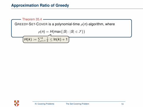
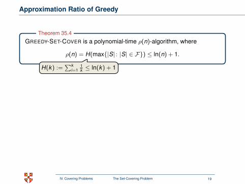
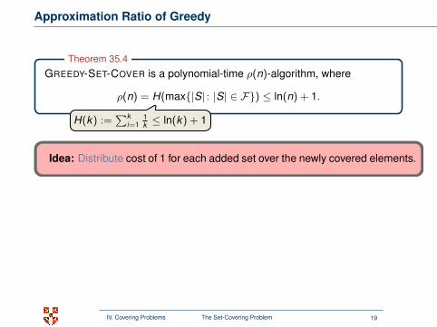
GREEDY-SET-COVER is a polynomial-time ρ(n)-algorithm, where
ρ(n) = H(max{|S| : |S| ∈ F})
≤ ln(n) + 1.
Theorem 35.4
H(k) :=∑k
i=11k ≤ ln(k) + 1
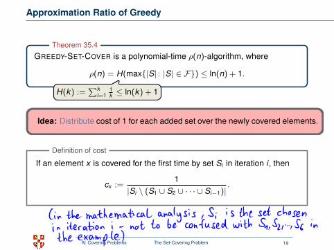
Idea: Distribute cost of 1 for each added set over the newly covered elements.
If an element x is covered for the first time by set Si in iteration i , then
cx :=1
|Si \ (S1 ∪ S2 ∪ · · · ∪ Si−1)|.
Definition of cost
IV. Covering Problems The Set-Covering Problem 19
Approximation Ratio of Greedy
GREEDY-SET-COVER is a polynomial-time ρ(n)-algorithm, where
ρ(n) = H(max{|S| : |S| ∈ F})
≤ ln(n) + 1.
Theorem 35.4
H(k) :=∑k
i=11k ≤ ln(k) + 1
Idea: Distribute cost of 1 for each added set over the newly covered elements.
If an element x is covered for the first time by set Si in iteration i , then
cx :=1
|Si \ (S1 ∪ S2 ∪ · · · ∪ Si−1)|.
Definition of cost
IV. Covering Problems The Set-Covering Problem 19
Approximation Ratio of Greedy
GREEDY-SET-COVER is a polynomial-time ρ(n)-algorithm, where
ρ(n) = H(max{|S| : |S| ∈ F}) ≤ ln(n) + 1.
Theorem 35.4
H(k) :=∑k
i=11k ≤ ln(k) + 1
Idea: Distribute cost of 1 for each added set over the newly covered elements.
If an element x is covered for the first time by set Si in iteration i , then
cx :=1
|Si \ (S1 ∪ S2 ∪ · · · ∪ Si−1)|.
Definition of cost
IV. Covering Problems The Set-Covering Problem 19
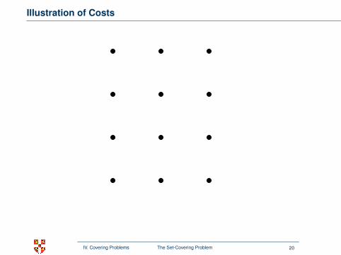
Illustration of Costs
S1
S2
S3 S4 S5
S6
S1
S4 S5S3
16
16
16
16
16
16
13
13
13
12
121
16 + 1
6 + 16 + 1
6 + 16 + 1
6 + 13 + 1
3 + 13 + 1
2 + 12 + 1 =
4
IV. Covering Problems The Set-Covering Problem 20
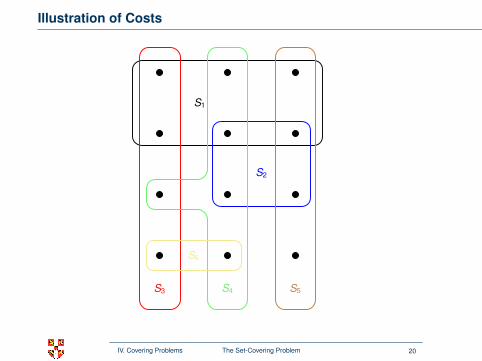
Illustration of Costs
S1
S2
S3 S4 S5
S6
S1
S4 S5S3
16
16
16
16
16
16
13
13
13
12
121
16 + 1
6 + 16 + 1
6 + 16 + 1
6 + 13 + 1
3 + 13 + 1
2 + 12 + 1 =
4
IV. Covering Problems The Set-Covering Problem 20
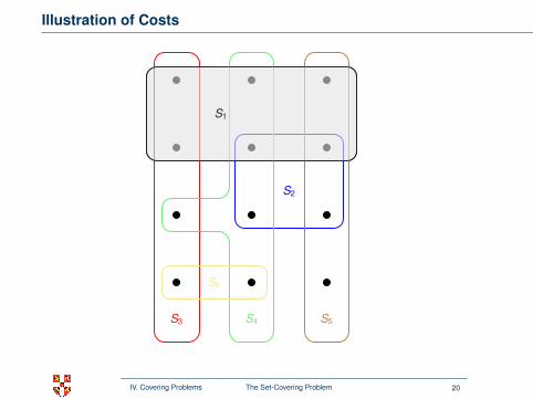
Illustration of Costs
S1
S2
S3 S4 S5
S6
S1
S4 S5S3
16
16
16
16
16
16
13
13
13
12
121
16 + 1
6 + 16 + 1
6 + 16 + 1
6 + 13 + 1
3 + 13 + 1
2 + 12 + 1 =
4
IV. Covering Problems The Set-Covering Problem 20
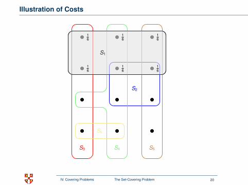
Illustration of Costs
S1
S2
S3 S4 S5
S6
S1
S4 S5S3
16
16
16
16
16
16
13
13
13
12
121
16 + 1
6 + 16 + 1
6 + 16 + 1
6 + 13 + 1
3 + 13 + 1
2 + 12 + 1 =
4
IV. Covering Problems The Set-Covering Problem 20

Illustration of Costs
S1
S2
S3 S4 S5
S6
S1
S4
S5S3
16
16
16
16
16
16
13
13
13
12
121
16 + 1
6 + 16 + 1
6 + 16 + 1
6 + 13 + 1
3 + 13 + 1
2 + 12 + 1 =
4
IV. Covering Problems The Set-Covering Problem 20
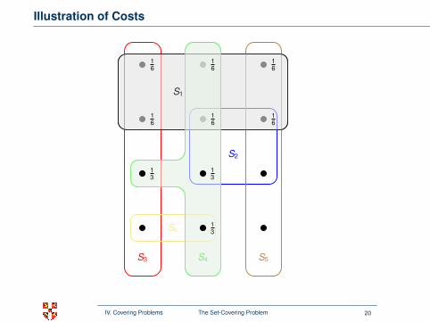
Illustration of Costs
S1
S2
S3 S4 S5
S6
S1
S4
S5S3
16
16
16
16
16
16
13
13
13
12
121
16 + 1
6 + 16 + 1
6 + 16 + 1
6 + 13 + 1
3 + 13 + 1
2 + 12 + 1 =
4
IV. Covering Problems The Set-Covering Problem 20
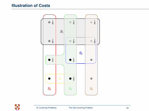
Illustration of Costs
S1
S2
S3 S4 S5
S6
S1
S4 S5
S3
16
16
16
16
16
16
13
13
13
12
121
16 + 1
6 + 16 + 1
6 + 16 + 1
6 + 13 + 1
3 + 13 + 1
2 + 12 + 1 =
4
IV. Covering Problems The Set-Covering Problem 20
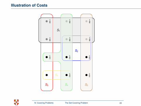
Illustration of Costs
S1
S2
S3 S4 S5
S6
S1
S4 S5
S3
16
16
16
16
16
16
13
13
13
12
12
1
16 + 1
6 + 16 + 1
6 + 16 + 1
6 + 13 + 1
3 + 13 + 1
2 + 12 + 1 =
4
IV. Covering Problems The Set-Covering Problem 20
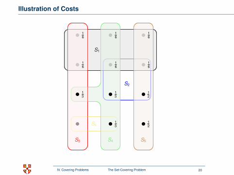
Illustration of Costs
S1
S2
S3 S4 S5
S6
S1
S4 S5S3
16
16
16
16
16
16
13
13
13
12
12
1
16 + 1
6 + 16 + 1
6 + 16 + 1
6 + 13 + 1
3 + 13 + 1
2 + 12 + 1 =
4
IV. Covering Problems The Set-Covering Problem 20
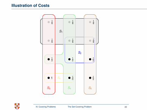
Illustration of Costs
S1
S2
S3 S4 S5
S6
S1
S4 S5S3
16
16
16
16
16
16
13
13
13
12
121
16 + 1
6 + 16 + 1
6 + 16 + 1
6 + 13 + 1
3 + 13 + 1
2 + 12 + 1 =
4
IV. Covering Problems The Set-Covering Problem 20
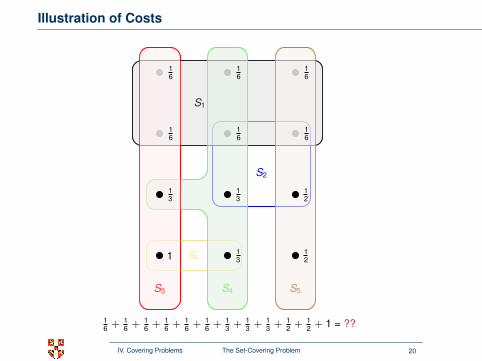
Illustration of Costs
S1
S2
S3 S4 S5
S6
S1
S4 S5S3
16
16
16
16
16
16
13
13
13
12
121
16 + 1
6 + 16 + 1
6 + 16 + 1
6 + 13 + 1
3 + 13 + 1
2 + 12 + 1 = ??
4
IV. Covering Problems The Set-Covering Problem 20

Illustration of Costs
S1
S2
S3 S4 S5
S6
S1
S4 S5S3
16
16
16
16
16
16
13
13
13
12
121
16 + 1
6 + 16 + 1
6 + 16 + 1
6 + 13 + 1
3 + 13 + 1
2 + 12 + 1 = 4
IV. Covering Problems The Set-Covering Problem 20
Proof of Theorem 35.4 (1/2)
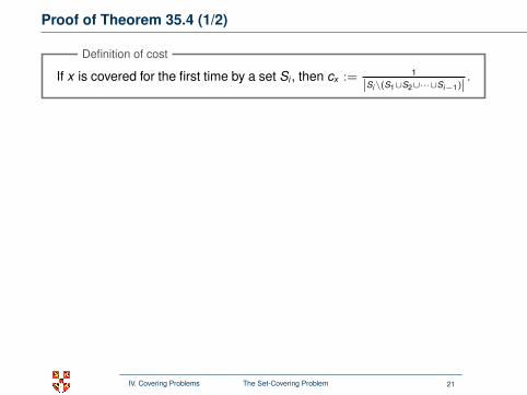
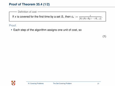
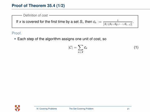
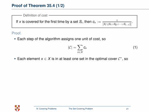
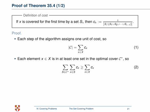
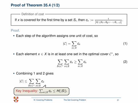
If x is covered for the first time by a set Si , then cx := 1
|Si\(S1∪S2∪···∪Si−1)|.
Definition of cost
Proof.
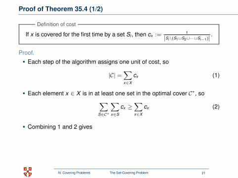
Each step of the algorithm assigns one unit of cost, so
|C| =∑x∈X
cx
(1)
Each element x ∈ X is in at least one set in the optimal cover C∗, so
∑S∈C∗
∑x∈S
cx ≥∑x∈X
cx (2)
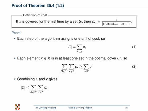
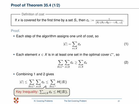
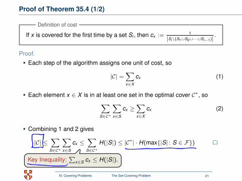
Combining 1 and 2 gives
|C| ≤∑
S∈C∗
∑x∈S
cx
≤∑
S∈C∗H(|S|) ≤ |C∗| · H(max{|S| : S ∈ F})
Key Inequality:∑
x∈S cx ≤ H(|S|).
IV. Covering Problems The Set-Covering Problem 21
Proof of Theorem 35.4 (1/2)
If x is covered for the first time by a set Si , then cx := 1
|Si\(S1∪S2∪···∪Si−1)|.
Definition of cost
Proof.
Each step of the algorithm assigns one unit of cost, so
|C| =∑x∈X
cx
(1)
Each element x ∈ X is in at least one set in the optimal cover C∗, so
∑S∈C∗
∑x∈S
cx ≥∑x∈X
cx (2)
Combining 1 and 2 gives
|C| ≤∑
S∈C∗
∑x∈S
cx
≤∑
S∈C∗H(|S|) ≤ |C∗| · H(max{|S| : S ∈ F})
Key Inequality:∑
x∈S cx ≤ H(|S|).
IV. Covering Problems The Set-Covering Problem 21
Proof of Theorem 35.4 (1/2)
If x is covered for the first time by a set Si , then cx := 1
|Si\(S1∪S2∪···∪Si−1)|.
Definition of cost
Proof.
Each step of the algorithm assigns one unit of cost, so
|C| =∑x∈X
cx (1)
Each element x ∈ X is in at least one set in the optimal cover C∗, so∑S∈C∗
∑x∈S
cx ≥∑x∈X
cx (2)
Combining 1 and 2 gives
|C| ≤∑
S∈C∗
∑x∈S
cx ≤∑
S∈C∗H(|S|)
≤ |C∗| · H(max{|S| : S ∈ F})
Key Inequality:∑
x∈S cx ≤ H(|S|).
IV. Covering Problems The Set-Covering Problem 21
Proof of Theorem 35.4 (1/2)
If x is covered for the first time by a set Si , then cx := 1
|Si\(S1∪S2∪···∪Si−1)|.
Definition of cost
Proof.
Each step of the algorithm assigns one unit of cost, so
|C| =∑x∈X
cx (1)
Each element x ∈ X is in at least one set in the optimal cover C∗, so∑S∈C∗
∑x∈S
cx ≥∑x∈X
cx (2)
Combining 1 and 2 gives
|C| ≤∑
S∈C∗
∑x∈S
cx ≤∑
S∈C∗H(|S|) ≤ |C∗| · H(max{|S| : S ∈ F})
Key Inequality:∑
x∈S cx ≤ H(|S|).
IV. Covering Problems The Set-Covering Problem 21
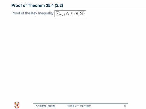
Proof of Theorem 35.4 (2/2)
Proof of the Key Inequality∑
x∈S cx ≤ H(|S|)
For any S ∈ F and i = 1, 2, . . . , |C| = k let
ui := |S \ (S1 ∪ S2 ∪ · · · ∪ Si )|
⇒ u0≥u1≥ · · ·≥u|C| = 0 and ui−1 − ui counts the items covered first time by Si .⇒ ∑
x∈S
cx
=k∑
i=1
(ui−1 − ui ) ·1
|Si \ (S1 ∪ S2 ∪ · · · ∪ Si−1)|
Further, by definition of the GREEDY-SET-COVER:
|Si \ (S1 ∪ S2 ∪ · · · ∪ Si−1)| ≥ |S \ (S1 ∪ S2 ∪ · · · ∪ Si−1)| = ui−1.
Combining the last inequalities gives:
∑x∈S
cx
≤k∑
i=1
(ui−1 − ui ) ·1
ui−1=
k∑i=1
ui−1∑j=ui+1
1ui−1
≤k∑
i=1
ui−1∑j=ui+1
1j
=k∑
i=1
(H(ui−1)− H(ui )) = H(u0)− H(uk ) = H(|S|).
Remaining uncovered elements in S Sets chosen by the algorithm
Each factor is at most one.
IV. Covering Problems The Set-Covering Problem 22
Proof of Theorem 35.4 (2/2)
Proof of the Key Inequality∑
x∈S cx ≤ H(|S|)
For any S ∈ F and i = 1, 2, . . . , |C| = k let
ui := |S \ (S1 ∪ S2 ∪ · · · ∪ Si )|⇒ u0≥u1≥ · · ·≥u|C| = 0 and ui−1 − ui counts the items covered first time by Si .⇒ ∑
x∈S
cx
=k∑
i=1
(ui−1 − ui ) ·1
|Si \ (S1 ∪ S2 ∪ · · · ∪ Si−1)|
Further, by definition of the GREEDY-SET-COVER:
|Si \ (S1 ∪ S2 ∪ · · · ∪ Si−1)| ≥ |S \ (S1 ∪ S2 ∪ · · · ∪ Si−1)| = ui−1.
Combining the last inequalities gives:
∑x∈S
cx
≤k∑
i=1
(ui−1 − ui ) ·1
ui−1=
k∑i=1
ui−1∑j=ui+1
1ui−1
≤k∑
i=1
ui−1∑j=ui+1
1j
=k∑
i=1
(H(ui−1)− H(ui )) = H(u0)− H(uk ) = H(|S|).
Remaining uncovered elements in S Sets chosen by the algorithm
Each factor is at most one.
IV. Covering Problems The Set-Covering Problem 22
Proof of Theorem 35.4 (2/2)
Proof of the Key Inequality∑
x∈S cx ≤ H(|S|)
For any S ∈ F and i = 1, 2, . . . , |C| = k let ui := |S \ (S1 ∪ S2 ∪ · · · ∪ Si )|
⇒ u0≥u1≥ · · ·≥u|C| = 0 and ui−1 − ui counts the items covered first time by Si .⇒ ∑
x∈S
cx
=k∑
i=1
(ui−1 − ui ) ·1
|Si \ (S1 ∪ S2 ∪ · · · ∪ Si−1)|
Further, by definition of the GREEDY-SET-COVER:
|Si \ (S1 ∪ S2 ∪ · · · ∪ Si−1)| ≥ |S \ (S1 ∪ S2 ∪ · · · ∪ Si−1)| = ui−1.
Combining the last inequalities gives:
∑x∈S
cx
≤k∑
i=1
(ui−1 − ui ) ·1
ui−1=
k∑i=1
ui−1∑j=ui+1
1ui−1
≤k∑
i=1
ui−1∑j=ui+1
1j
=k∑
i=1
(H(ui−1)− H(ui )) = H(u0)− H(uk ) = H(|S|).
Remaining uncovered elements in S Sets chosen by the algorithm
Each factor is at most one.
IV. Covering Problems The Set-Covering Problem 22

Proof of Theorem 35.4 (2/2)
Proof of the Key Inequality∑
x∈S cx ≤ H(|S|)
For any S ∈ F and i = 1, 2, . . . , |C| = k let ui := |S \ (S1 ∪ S2 ∪ · · · ∪ Si )|
⇒ u0≥u1≥ · · ·≥u|C| = 0 and ui−1 − ui counts the items covered first time by Si .⇒ ∑
x∈S
cx
=k∑
i=1
(ui−1 − ui ) ·1
|Si \ (S1 ∪ S2 ∪ · · · ∪ Si−1)|
Further, by definition of the GREEDY-SET-COVER:
|Si \ (S1 ∪ S2 ∪ · · · ∪ Si−1)| ≥ |S \ (S1 ∪ S2 ∪ · · · ∪ Si−1)| = ui−1.
Combining the last inequalities gives:
∑x∈S
cx
≤k∑
i=1
(ui−1 − ui ) ·1
ui−1=
k∑i=1
ui−1∑j=ui+1
1ui−1
≤k∑
i=1
ui−1∑j=ui+1
1j
=k∑
i=1
(H(ui−1)− H(ui )) = H(u0)− H(uk ) = H(|S|).
Remaining uncovered elements in S
Sets chosen by the algorithm
Each factor is at most one.
IV. Covering Problems The Set-Covering Problem 22
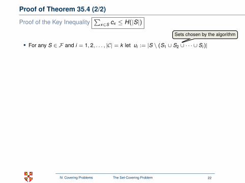
Proof of Theorem 35.4 (2/2)
Proof of the Key Inequality∑
x∈S cx ≤ H(|S|)
For any S ∈ F and i = 1, 2, . . . , |C| = k let ui := |S \ (S1 ∪ S2 ∪ · · · ∪ Si )|
⇒ u0≥u1≥ · · ·≥u|C| = 0 and ui−1 − ui counts the items covered first time by Si .⇒ ∑
x∈S
cx
=k∑
i=1
(ui−1 − ui ) ·1
|Si \ (S1 ∪ S2 ∪ · · · ∪ Si−1)|
Further, by definition of the GREEDY-SET-COVER:
|Si \ (S1 ∪ S2 ∪ · · · ∪ Si−1)| ≥ |S \ (S1 ∪ S2 ∪ · · · ∪ Si−1)| = ui−1.
Combining the last inequalities gives:
∑x∈S
cx
≤k∑
i=1
(ui−1 − ui ) ·1
ui−1=
k∑i=1
ui−1∑j=ui+1
1ui−1
≤k∑
i=1
ui−1∑j=ui+1
1j
=k∑
i=1
(H(ui−1)− H(ui )) = H(u0)− H(uk ) = H(|S|).
Remaining uncovered elements in S
Sets chosen by the algorithm
Each factor is at most one.
IV. Covering Problems The Set-Covering Problem 22
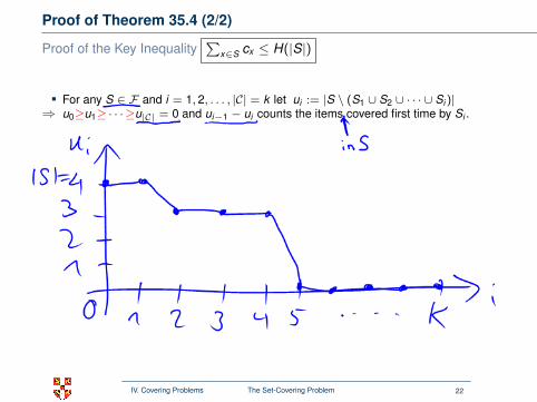
Proof of Theorem 35.4 (2/2)
Proof of the Key Inequality∑
x∈S cx ≤ H(|S|)
For any S ∈ F and i = 1, 2, . . . , |C| = k let ui := |S \ (S1 ∪ S2 ∪ · · · ∪ Si )|⇒ u0≥u1≥ · · ·≥u|C| = 0 and ui−1 − ui counts the items covered first time by Si .
⇒ ∑x∈S
cx
=k∑
i=1
(ui−1 − ui ) ·1
|Si \ (S1 ∪ S2 ∪ · · · ∪ Si−1)|
Further, by definition of the GREEDY-SET-COVER:
|Si \ (S1 ∪ S2 ∪ · · · ∪ Si−1)| ≥ |S \ (S1 ∪ S2 ∪ · · · ∪ Si−1)| = ui−1.
Combining the last inequalities gives:
∑x∈S
cx
≤k∑
i=1
(ui−1 − ui ) ·1
ui−1=
k∑i=1
ui−1∑j=ui+1
1ui−1
≤k∑
i=1
ui−1∑j=ui+1
1j
=k∑
i=1
(H(ui−1)− H(ui )) = H(u0)− H(uk ) = H(|S|).
Remaining uncovered elements in S Sets chosen by the algorithm
Each factor is at most one.
IV. Covering Problems The Set-Covering Problem 22
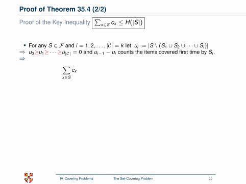
Proof of Theorem 35.4 (2/2)
Proof of the Key Inequality∑
x∈S cx ≤ H(|S|)
For any S ∈ F and i = 1, 2, . . . , |C| = k let ui := |S \ (S1 ∪ S2 ∪ · · · ∪ Si )|⇒ u0≥u1≥ · · ·≥u|C| = 0 and ui−1 − ui counts the items covered first time by Si .⇒ ∑
x∈S
cx
=k∑
i=1
(ui−1 − ui ) ·1
|Si \ (S1 ∪ S2 ∪ · · · ∪ Si−1)|
Further, by definition of the GREEDY-SET-COVER:
|Si \ (S1 ∪ S2 ∪ · · · ∪ Si−1)| ≥ |S \ (S1 ∪ S2 ∪ · · · ∪ Si−1)| = ui−1.
Combining the last inequalities gives:
∑x∈S
cx
≤k∑
i=1
(ui−1 − ui ) ·1
ui−1=
k∑i=1
ui−1∑j=ui+1
1ui−1
≤k∑
i=1
ui−1∑j=ui+1
1j
=k∑
i=1
(H(ui−1)− H(ui )) = H(u0)− H(uk ) = H(|S|).
Remaining uncovered elements in S Sets chosen by the algorithm
Each factor is at most one.
IV. Covering Problems The Set-Covering Problem 22
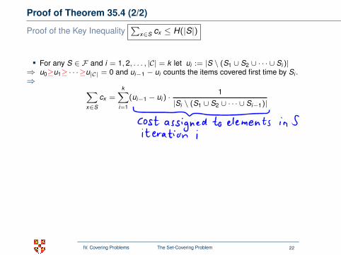
Proof of Theorem 35.4 (2/2)
Proof of the Key Inequality∑
x∈S cx ≤ H(|S|)
For any S ∈ F and i = 1, 2, . . . , |C| = k let ui := |S \ (S1 ∪ S2 ∪ · · · ∪ Si )|⇒ u0≥u1≥ · · ·≥u|C| = 0 and ui−1 − ui counts the items covered first time by Si .⇒ ∑
x∈S
cx =k∑
i=1
(ui−1 − ui ) ·1
|Si \ (S1 ∪ S2 ∪ · · · ∪ Si−1)|
Further, by definition of the GREEDY-SET-COVER:
|Si \ (S1 ∪ S2 ∪ · · · ∪ Si−1)| ≥ |S \ (S1 ∪ S2 ∪ · · · ∪ Si−1)| = ui−1.
Combining the last inequalities gives:
∑x∈S
cx
≤k∑
i=1
(ui−1 − ui ) ·1
ui−1=
k∑i=1
ui−1∑j=ui+1
1ui−1
≤k∑
i=1
ui−1∑j=ui+1
1j
=k∑
i=1
(H(ui−1)− H(ui )) = H(u0)− H(uk ) = H(|S|).
Remaining uncovered elements in S Sets chosen by the algorithm
Each factor is at most one.
IV. Covering Problems The Set-Covering Problem 22
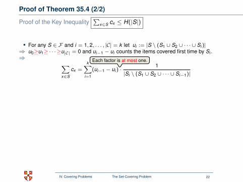
Proof of Theorem 35.4 (2/2)
Proof of the Key Inequality∑
x∈S cx ≤ H(|S|)
For any S ∈ F and i = 1, 2, . . . , |C| = k let ui := |S \ (S1 ∪ S2 ∪ · · · ∪ Si )|⇒ u0≥u1≥ · · ·≥u|C| = 0 and ui−1 − ui counts the items covered first time by Si .⇒ ∑
x∈S
cx =k∑
i=1
(ui−1 − ui ) ·1
|Si \ (S1 ∪ S2 ∪ · · · ∪ Si−1)|
Further, by definition of the GREEDY-SET-COVER:
|Si \ (S1 ∪ S2 ∪ · · · ∪ Si−1)| ≥ |S \ (S1 ∪ S2 ∪ · · · ∪ Si−1)| = ui−1.
Combining the last inequalities gives:
∑x∈S
cx
≤k∑
i=1
(ui−1 − ui ) ·1
ui−1=
k∑i=1
ui−1∑j=ui+1
1ui−1
≤k∑
i=1
ui−1∑j=ui+1
1j
=k∑
i=1
(H(ui−1)− H(ui )) = H(u0)− H(uk ) = H(|S|).
Remaining uncovered elements in S Sets chosen by the algorithm
Each factor is at most one.
IV. Covering Problems The Set-Covering Problem 22
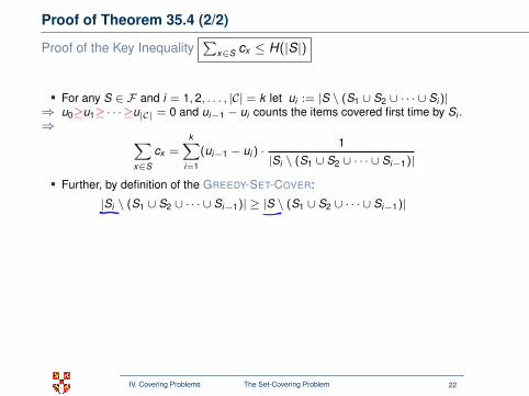
Proof of Theorem 35.4 (2/2)
Proof of the Key Inequality∑
x∈S cx ≤ H(|S|)
For any S ∈ F and i = 1, 2, . . . , |C| = k let ui := |S \ (S1 ∪ S2 ∪ · · · ∪ Si )|⇒ u0≥u1≥ · · ·≥u|C| = 0 and ui−1 − ui counts the items covered first time by Si .⇒ ∑
x∈S
cx =k∑
i=1
(ui−1 − ui ) ·1
|Si \ (S1 ∪ S2 ∪ · · · ∪ Si−1)|
Further, by definition of the GREEDY-SET-COVER:
|Si \ (S1 ∪ S2 ∪ · · · ∪ Si−1)| ≥ |S \ (S1 ∪ S2 ∪ · · · ∪ Si−1)|
= ui−1.
Combining the last inequalities gives:
∑x∈S
cx
≤k∑
i=1
(ui−1 − ui ) ·1
ui−1=
k∑i=1
ui−1∑j=ui+1
1ui−1
≤k∑
i=1
ui−1∑j=ui+1
1j
=k∑
i=1
(H(ui−1)− H(ui )) = H(u0)− H(uk ) = H(|S|).
Remaining uncovered elements in S Sets chosen by the algorithm
Each factor is at most one.
IV. Covering Problems The Set-Covering Problem 22
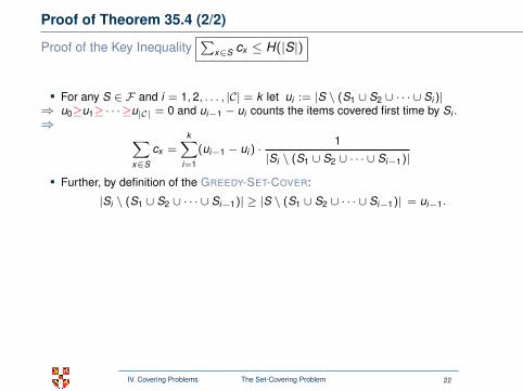
Proof of Theorem 35.4 (2/2)
Proof of the Key Inequality∑
x∈S cx ≤ H(|S|)
For any S ∈ F and i = 1, 2, . . . , |C| = k let ui := |S \ (S1 ∪ S2 ∪ · · · ∪ Si )|⇒ u0≥u1≥ · · ·≥u|C| = 0 and ui−1 − ui counts the items covered first time by Si .⇒ ∑
x∈S
cx =k∑
i=1
(ui−1 − ui ) ·1
|Si \ (S1 ∪ S2 ∪ · · · ∪ Si−1)|
Further, by definition of the GREEDY-SET-COVER:
|Si \ (S1 ∪ S2 ∪ · · · ∪ Si−1)| ≥ |S \ (S1 ∪ S2 ∪ · · · ∪ Si−1)| = ui−1.
Combining the last inequalities gives:
∑x∈S
cx
≤k∑
i=1
(ui−1 − ui ) ·1
ui−1=
k∑i=1
ui−1∑j=ui+1
1ui−1
≤k∑
i=1
ui−1∑j=ui+1
1j
=k∑
i=1
(H(ui−1)− H(ui )) = H(u0)− H(uk ) = H(|S|).
Remaining uncovered elements in S Sets chosen by the algorithm
Each factor is at most one.
IV. Covering Problems The Set-Covering Problem 22

Proof of Theorem 35.4 (2/2)
Proof of the Key Inequality∑
x∈S cx ≤ H(|S|)
For any S ∈ F and i = 1, 2, . . . , |C| = k let ui := |S \ (S1 ∪ S2 ∪ · · · ∪ Si )|⇒ u0≥u1≥ · · ·≥u|C| = 0 and ui−1 − ui counts the items covered first time by Si .⇒ ∑
x∈S
cx =k∑
i=1
(ui−1 − ui ) ·1
|Si \ (S1 ∪ S2 ∪ · · · ∪ Si−1)|
Further, by definition of the GREEDY-SET-COVER:
|Si \ (S1 ∪ S2 ∪ · · · ∪ Si−1)| ≥ |S \ (S1 ∪ S2 ∪ · · · ∪ Si−1)| = ui−1.
Combining the last inequalities gives:
∑x∈S
cx
≤k∑
i=1
(ui−1 − ui ) ·1
ui−1=
k∑i=1
ui−1∑j=ui+1
1ui−1
≤k∑
i=1
ui−1∑j=ui+1
1j
=k∑
i=1
(H(ui−1)− H(ui )) = H(u0)− H(uk ) = H(|S|).
Remaining uncovered elements in S Sets chosen by the algorithm
Each factor is at most one.
IV. Covering Problems The Set-Covering Problem 22
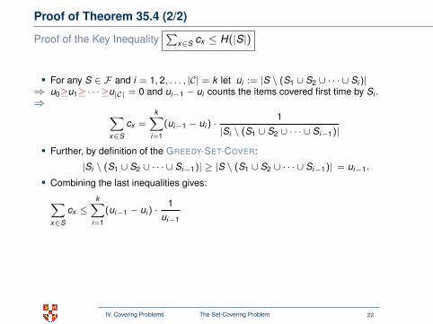
Proof of Theorem 35.4 (2/2)
Proof of the Key Inequality∑
x∈S cx ≤ H(|S|)
For any S ∈ F and i = 1, 2, . . . , |C| = k let ui := |S \ (S1 ∪ S2 ∪ · · · ∪ Si )|⇒ u0≥u1≥ · · ·≥u|C| = 0 and ui−1 − ui counts the items covered first time by Si .⇒ ∑
x∈S
cx =k∑
i=1
(ui−1 − ui ) ·1
|Si \ (S1 ∪ S2 ∪ · · · ∪ Si−1)|
Further, by definition of the GREEDY-SET-COVER:
|Si \ (S1 ∪ S2 ∪ · · · ∪ Si−1)| ≥ |S \ (S1 ∪ S2 ∪ · · · ∪ Si−1)| = ui−1.
Combining the last inequalities gives:
∑x∈S
cx ≤k∑
i=1
(ui−1 − ui ) ·1
ui−1
=k∑
i=1
ui−1∑j=ui+1
1ui−1
≤k∑
i=1
ui−1∑j=ui+1
1j
=k∑
i=1
(H(ui−1)− H(ui )) = H(u0)− H(uk ) = H(|S|).
Remaining uncovered elements in S Sets chosen by the algorithm
Each factor is at most one.
IV. Covering Problems The Set-Covering Problem 22
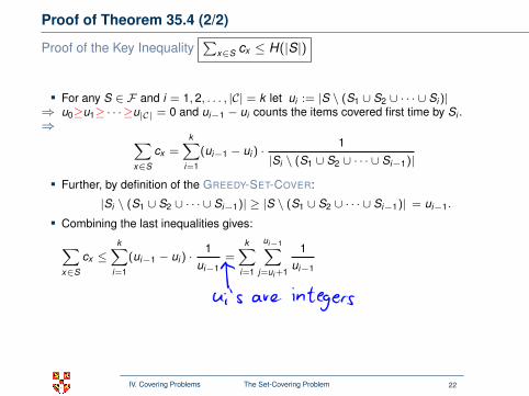
Proof of Theorem 35.4 (2/2)
Proof of the Key Inequality∑
x∈S cx ≤ H(|S|)
For any S ∈ F and i = 1, 2, . . . , |C| = k let ui := |S \ (S1 ∪ S2 ∪ · · · ∪ Si )|⇒ u0≥u1≥ · · ·≥u|C| = 0 and ui−1 − ui counts the items covered first time by Si .⇒ ∑
x∈S
cx =k∑
i=1
(ui−1 − ui ) ·1
|Si \ (S1 ∪ S2 ∪ · · · ∪ Si−1)|
Further, by definition of the GREEDY-SET-COVER:
|Si \ (S1 ∪ S2 ∪ · · · ∪ Si−1)| ≥ |S \ (S1 ∪ S2 ∪ · · · ∪ Si−1)| = ui−1.
Combining the last inequalities gives:
∑x∈S
cx ≤k∑
i=1
(ui−1 − ui ) ·1
ui−1=
k∑i=1
ui−1∑j=ui+1
1ui−1
≤k∑
i=1
ui−1∑j=ui+1
1j
=k∑
i=1
(H(ui−1)− H(ui )) = H(u0)− H(uk ) = H(|S|).
Remaining uncovered elements in S Sets chosen by the algorithm
Each factor is at most one.
IV. Covering Problems The Set-Covering Problem 22
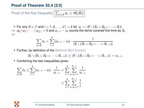
Proof of Theorem 35.4 (2/2)
Proof of the Key Inequality∑
x∈S cx ≤ H(|S|)
For any S ∈ F and i = 1, 2, . . . , |C| = k let ui := |S \ (S1 ∪ S2 ∪ · · · ∪ Si )|⇒ u0≥u1≥ · · ·≥u|C| = 0 and ui−1 − ui counts the items covered first time by Si .⇒ ∑
x∈S
cx =k∑
i=1
(ui−1 − ui ) ·1
|Si \ (S1 ∪ S2 ∪ · · · ∪ Si−1)|
Further, by definition of the GREEDY-SET-COVER:
|Si \ (S1 ∪ S2 ∪ · · · ∪ Si−1)| ≥ |S \ (S1 ∪ S2 ∪ · · · ∪ Si−1)| = ui−1.
Combining the last inequalities gives:
∑x∈S
cx ≤k∑
i=1
(ui−1 − ui ) ·1
ui−1=
k∑i=1
ui−1∑j=ui+1
1ui−1
≤k∑
i=1
ui−1∑j=ui+1
1j
=k∑
i=1
(H(ui−1)− H(ui )) = H(u0)− H(uk ) = H(|S|).
Remaining uncovered elements in S Sets chosen by the algorithm
Each factor is at most one.
IV. Covering Problems The Set-Covering Problem 22
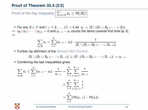
Proof of Theorem 35.4 (2/2)
Proof of the Key Inequality∑
x∈S cx ≤ H(|S|)
For any S ∈ F and i = 1, 2, . . . , |C| = k let ui := |S \ (S1 ∪ S2 ∪ · · · ∪ Si )|⇒ u0≥u1≥ · · ·≥u|C| = 0 and ui−1 − ui counts the items covered first time by Si .⇒ ∑
x∈S
cx =k∑
i=1
(ui−1 − ui ) ·1
|Si \ (S1 ∪ S2 ∪ · · · ∪ Si−1)|
Further, by definition of the GREEDY-SET-COVER:
|Si \ (S1 ∪ S2 ∪ · · · ∪ Si−1)| ≥ |S \ (S1 ∪ S2 ∪ · · · ∪ Si−1)| = ui−1.
Combining the last inequalities gives:
∑x∈S
cx ≤k∑
i=1
(ui−1 − ui ) ·1
ui−1=
k∑i=1
ui−1∑j=ui+1
1ui−1
≤k∑
i=1
ui−1∑j=ui+1
1j
=k∑
i=1
(H(ui−1)− H(ui ))
= H(u0)− H(uk ) = H(|S|).
Remaining uncovered elements in S Sets chosen by the algorithm
Each factor is at most one.
IV. Covering Problems The Set-Covering Problem 22
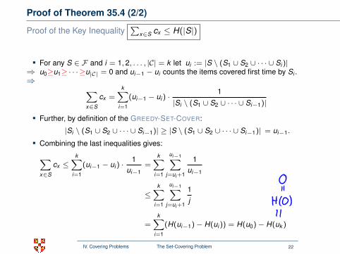
Proof of Theorem 35.4 (2/2)
Proof of the Key Inequality∑
x∈S cx ≤ H(|S|)
For any S ∈ F and i = 1, 2, . . . , |C| = k let ui := |S \ (S1 ∪ S2 ∪ · · · ∪ Si )|⇒ u0≥u1≥ · · ·≥u|C| = 0 and ui−1 − ui counts the items covered first time by Si .⇒ ∑
x∈S
cx =k∑
i=1
(ui−1 − ui ) ·1
|Si \ (S1 ∪ S2 ∪ · · · ∪ Si−1)|
Further, by definition of the GREEDY-SET-COVER:
|Si \ (S1 ∪ S2 ∪ · · · ∪ Si−1)| ≥ |S \ (S1 ∪ S2 ∪ · · · ∪ Si−1)| = ui−1.
Combining the last inequalities gives:
∑x∈S
cx ≤k∑
i=1
(ui−1 − ui ) ·1
ui−1=
k∑i=1
ui−1∑j=ui+1
1ui−1
≤k∑
i=1
ui−1∑j=ui+1
1j
=k∑
i=1
(H(ui−1)− H(ui )) = H(u0)− H(uk )
= H(|S|).
Remaining uncovered elements in S Sets chosen by the algorithm
Each factor is at most one.
IV. Covering Problems The Set-Covering Problem 22
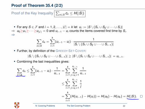
Proof of Theorem 35.4 (2/2)
Proof of the Key Inequality∑
x∈S cx ≤ H(|S|)
For any S ∈ F and i = 1, 2, . . . , |C| = k let ui := |S \ (S1 ∪ S2 ∪ · · · ∪ Si )|⇒ u0≥u1≥ · · ·≥u|C| = 0 and ui−1 − ui counts the items covered first time by Si .⇒ ∑
x∈S
cx =k∑
i=1
(ui−1 − ui ) ·1
|Si \ (S1 ∪ S2 ∪ · · · ∪ Si−1)|
Further, by definition of the GREEDY-SET-COVER:
|Si \ (S1 ∪ S2 ∪ · · · ∪ Si−1)| ≥ |S \ (S1 ∪ S2 ∪ · · · ∪ Si−1)| = ui−1.
Combining the last inequalities gives:
∑x∈S
cx ≤k∑
i=1
(ui−1 − ui ) ·1
ui−1=
k∑i=1
ui−1∑j=ui+1
1ui−1
≤k∑
i=1
ui−1∑j=ui+1
1j
=k∑
i=1
(H(ui−1)− H(ui )) = H(u0)− H(uk ) = H(|S|).
Remaining uncovered elements in S Sets chosen by the algorithm
Each factor is at most one.
IV. Covering Problems The Set-Covering Problem 22
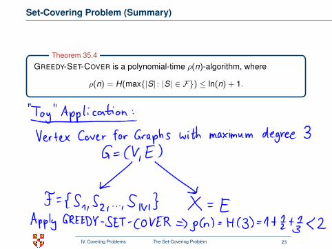
Set-Covering Problem (Summary)
GREEDY-SET-COVER is a polynomial-time ρ(n)-algorithm, where
ρ(n) = H(max{|S| : |S| ∈ F}) ≤ ln(n) + 1.
Theorem 35.4
The same approach also gives an approximation ratioof O(ln(n)) if there exists a cost function c : S → Z+
Is the bound on the approximation ratio tight?
Is there a better algorithm?
Unless P=NP, there is no c · ln(n) approximation algorithm for set coverfor some constant 0 < c < 1.
Lower Bound
IV. Covering Problems The Set-Covering Problem 23
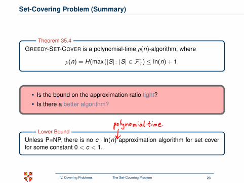
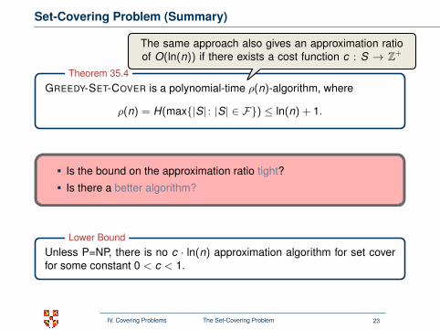

Example where Greedy is a (1/2) · log2 n factor off
Given any integer k ≥ 3
There are n = 2k+1 − 2 elements overall
Sets S1,S2, . . . ,Sk are pairwise disjoint and each set contains2, 4, . . . , 2k elements
Sets T1,T2 are disjoint and each set contains half of the elements ofeach set S1,S2, . . . ,Sk
Instance
k = 4:
S1 S2 S3 S4
Solution of Greedy consists of k sets. Optimum consists of 2 sets.
T1
T2
S1 S2 S3 S4
T1
T2
IV. Covering Problems The Set-Covering Problem 24
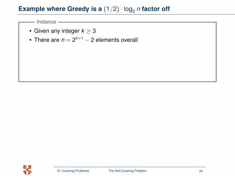
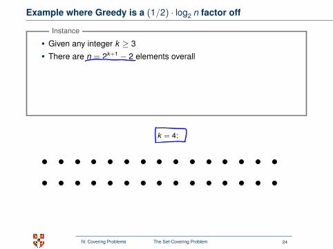
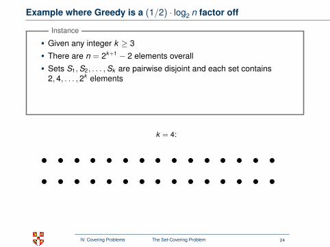
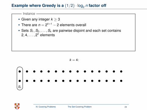
Example where Greedy is a (1/2) · log2 n factor off
Given any integer k ≥ 3
There are n = 2k+1 − 2 elements overall
Sets S1,S2, . . . ,Sk are pairwise disjoint and each set contains2, 4, . . . , 2k elements
Sets T1,T2 are disjoint and each set contains half of the elements ofeach set S1,S2, . . . ,Sk
Instance
k = 4:
S1
S2 S3 S4
Solution of Greedy consists of k sets. Optimum consists of 2 sets.
T1
T2
S1 S2 S3 S4
T1
T2
IV. Covering Problems The Set-Covering Problem 24
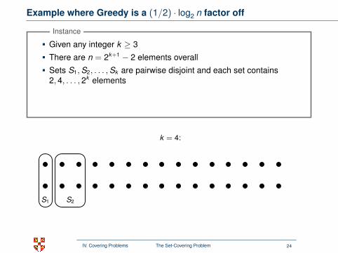
Example where Greedy is a (1/2) · log2 n factor off
Given any integer k ≥ 3
There are n = 2k+1 − 2 elements overall
Sets S1,S2, . . . ,Sk are pairwise disjoint and each set contains2, 4, . . . , 2k elements
Sets T1,T2 are disjoint and each set contains half of the elements ofeach set S1,S2, . . . ,Sk
Instance
k = 4:
S1 S2
S3 S4
Solution of Greedy consists of k sets. Optimum consists of 2 sets.
T1
T2
S1 S2 S3 S4
T1
T2
IV. Covering Problems The Set-Covering Problem 24
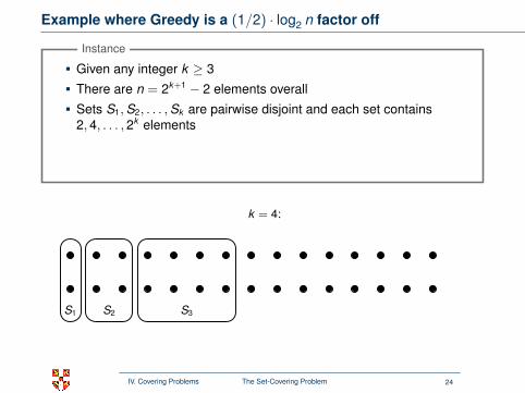
Example where Greedy is a (1/2) · log2 n factor off
Given any integer k ≥ 3
There are n = 2k+1 − 2 elements overall
Sets S1,S2, . . . ,Sk are pairwise disjoint and each set contains2, 4, . . . , 2k elements
Sets T1,T2 are disjoint and each set contains half of the elements ofeach set S1,S2, . . . ,Sk
Instance
k = 4:
S1 S2 S3
S4
Solution of Greedy consists of k sets. Optimum consists of 2 sets.
T1
T2
S1 S2 S3 S4
T1
T2
IV. Covering Problems The Set-Covering Problem 24
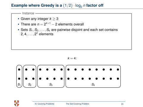
Example where Greedy is a (1/2) · log2 n factor off
Given any integer k ≥ 3
There are n = 2k+1 − 2 elements overall
Sets S1,S2, . . . ,Sk are pairwise disjoint and each set contains2, 4, . . . , 2k elements
Sets T1,T2 are disjoint and each set contains half of the elements ofeach set S1,S2, . . . ,Sk
Instance
k = 4:
S1 S2 S3 S4
Solution of Greedy consists of k sets. Optimum consists of 2 sets.
T1
T2
S1 S2 S3 S4
T1
T2
IV. Covering Problems The Set-Covering Problem 24
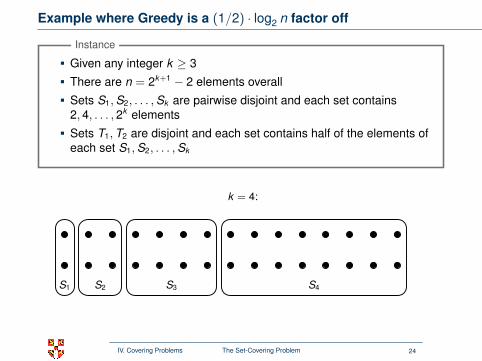
Example where Greedy is a (1/2) · log2 n factor off
Given any integer k ≥ 3
There are n = 2k+1 − 2 elements overall
Sets S1,S2, . . . ,Sk are pairwise disjoint and each set contains2, 4, . . . , 2k elements
Sets T1,T2 are disjoint and each set contains half of the elements ofeach set S1,S2, . . . ,Sk
Instance
k = 4:
S1 S2 S3 S4
Solution of Greedy consists of k sets. Optimum consists of 2 sets.
T1
T2
S1 S2 S3 S4
T1
T2
IV. Covering Problems The Set-Covering Problem 24
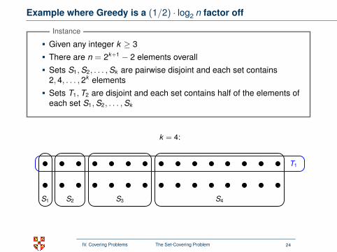
Example where Greedy is a (1/2) · log2 n factor off
Given any integer k ≥ 3
There are n = 2k+1 − 2 elements overall
Sets S1,S2, . . . ,Sk are pairwise disjoint and each set contains2, 4, . . . , 2k elements
Sets T1,T2 are disjoint and each set contains half of the elements ofeach set S1,S2, . . . ,Sk
Instance
k = 4:
S1 S2 S3 S4
Solution of Greedy consists of k sets. Optimum consists of 2 sets.
T1
T2
S1 S2 S3 S4
T1
T2
IV. Covering Problems The Set-Covering Problem 24
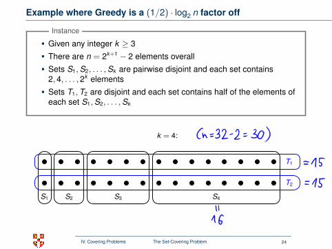
Example where Greedy is a (1/2) · log2 n factor off
Given any integer k ≥ 3
There are n = 2k+1 − 2 elements overall
Sets S1,S2, . . . ,Sk are pairwise disjoint and each set contains2, 4, . . . , 2k elements
Sets T1,T2 are disjoint and each set contains half of the elements ofeach set S1,S2, . . . ,Sk
Instance
k = 4:
S1 S2 S3 S4
Solution of Greedy consists of k sets. Optimum consists of 2 sets.
T1
T2
S1 S2 S3 S4
T1
T2
IV. Covering Problems The Set-Covering Problem 24
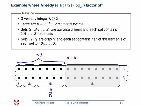
Example where Greedy is a (1/2) · log2 n factor off
Given any integer k ≥ 3
There are n = 2k+1 − 2 elements overall
Sets S1,S2, . . . ,Sk are pairwise disjoint and each set contains2, 4, . . . , 2k elements
Sets T1,T2 are disjoint and each set contains half of the elements ofeach set S1,S2, . . . ,Sk
Instance
k = 4:
S1 S2 S3 S4
Solution of Greedy consists of k sets. Optimum consists of 2 sets.
T1
T2
S1 S2 S3
S4
T1
T2
IV. Covering Problems The Set-Covering Problem 24
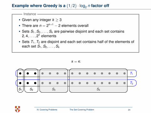
Example where Greedy is a (1/2) · log2 n factor off
Given any integer k ≥ 3
There are n = 2k+1 − 2 elements overall
Sets S1,S2, . . . ,Sk are pairwise disjoint and each set contains2, 4, . . . , 2k elements
Sets T1,T2 are disjoint and each set contains half of the elements ofeach set S1,S2, . . . ,Sk
Instance
k = 4:
S1 S2 S3 S4
Solution of Greedy consists of k sets. Optimum consists of 2 sets.
T1
T2
S1 S2
S3 S4
T1
T2
IV. Covering Problems The Set-Covering Problem 24
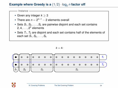
Example where Greedy is a (1/2) · log2 n factor off
Given any integer k ≥ 3
There are n = 2k+1 − 2 elements overall
Sets S1,S2, . . . ,Sk are pairwise disjoint and each set contains2, 4, . . . , 2k elements
Sets T1,T2 are disjoint and each set contains half of the elements ofeach set S1,S2, . . . ,Sk
Instance
k = 4:
S1 S2 S3 S4
Solution of Greedy consists of k sets. Optimum consists of 2 sets.
T1
T2
S1
S2 S3 S4
T1
T2
IV. Covering Problems The Set-Covering Problem 24
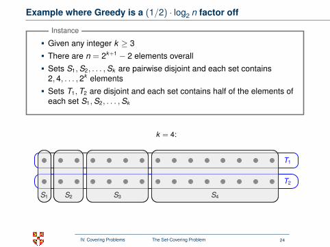
Example where Greedy is a (1/2) · log2 n factor off
Given any integer k ≥ 3
There are n = 2k+1 − 2 elements overall
Sets S1,S2, . . . ,Sk are pairwise disjoint and each set contains2, 4, . . . , 2k elements
Sets T1,T2 are disjoint and each set contains half of the elements ofeach set S1,S2, . . . ,Sk
Instance
k = 4:
S1 S2 S3 S4
Solution of Greedy consists of k sets. Optimum consists of 2 sets.
T1
T2
S1 S2 S3 S4
T1
T2
IV. Covering Problems The Set-Covering Problem 24
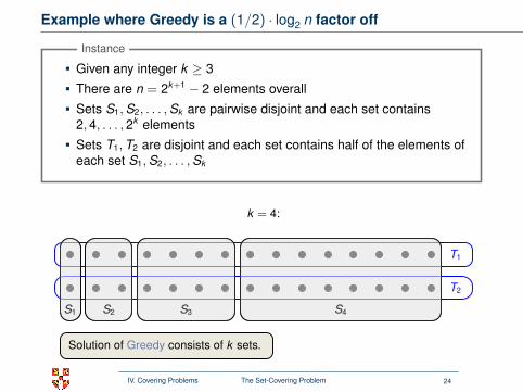
Example where Greedy is a (1/2) · log2 n factor off
Given any integer k ≥ 3
There are n = 2k+1 − 2 elements overall
Sets S1,S2, . . . ,Sk are pairwise disjoint and each set contains2, 4, . . . , 2k elements
Sets T1,T2 are disjoint and each set contains half of the elements ofeach set S1,S2, . . . ,Sk
Instance
k = 4:
S1 S2 S3 S4
Solution of Greedy consists of k sets.
Optimum consists of 2 sets.
T1
T2
S1 S2 S3 S4
T1
T2
IV. Covering Problems The Set-Covering Problem 24
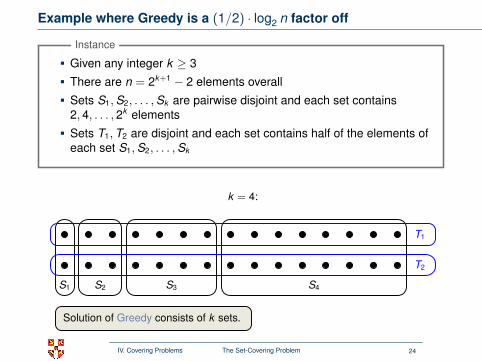
Example where Greedy is a (1/2) · log2 n factor off
Given any integer k ≥ 3
There are n = 2k+1 − 2 elements overall
Sets S1,S2, . . . ,Sk are pairwise disjoint and each set contains2, 4, . . . , 2k elements
Sets T1,T2 are disjoint and each set contains half of the elements ofeach set S1,S2, . . . ,Sk
Instance
k = 4:
S1 S2 S3 S4
Solution of Greedy consists of k sets.
Optimum consists of 2 sets.
T1
T2
S1 S2 S3 S4
T1
T2
IV. Covering Problems The Set-Covering Problem 24
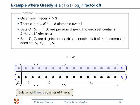
Example where Greedy is a (1/2) · log2 n factor off
Given any integer k ≥ 3
There are n = 2k+1 − 2 elements overall
Sets S1,S2, . . . ,Sk are pairwise disjoint and each set contains2, 4, . . . , 2k elements
Sets T1,T2 are disjoint and each set contains half of the elements ofeach set S1,S2, . . . ,Sk
Instance
k = 4:
S1 S2 S3 S4
Solution of Greedy consists of k sets.
Optimum consists of 2 sets.
T1
T2
S1 S2 S3 S4
T1
T2
IV. Covering Problems The Set-Covering Problem 24
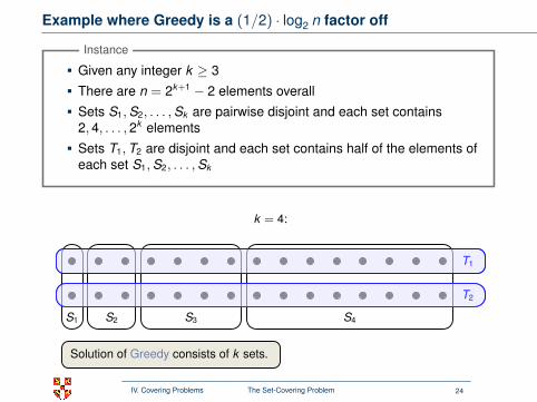
Example where Greedy is a (1/2) · log2 n factor off
Given any integer k ≥ 3
There are n = 2k+1 − 2 elements overall
Sets S1,S2, . . . ,Sk are pairwise disjoint and each set contains2, 4, . . . , 2k elements
Sets T1,T2 are disjoint and each set contains half of the elements ofeach set S1,S2, . . . ,Sk
Instance
k = 4:
S1 S2 S3 S4
Solution of Greedy consists of k sets.
Optimum consists of 2 sets.
T1
T2
S1 S2 S3 S4
T1
T2
IV. Covering Problems The Set-Covering Problem 24
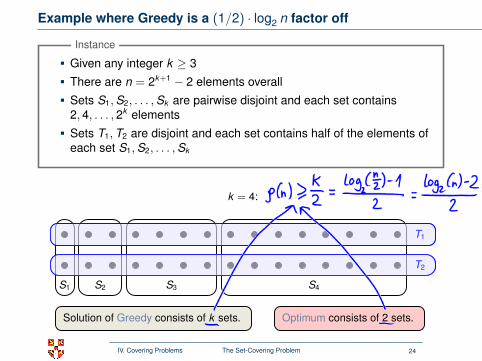
Example where Greedy is a (1/2) · log2 n factor off
Given any integer k ≥ 3
There are n = 2k+1 − 2 elements overall
Sets S1,S2, . . . ,Sk are pairwise disjoint and each set contains2, 4, . . . , 2k elements
Sets T1,T2 are disjoint and each set contains half of the elements ofeach set S1,S2, . . . ,Sk
Instance
k = 4:
S1 S2 S3 S4
Solution of Greedy consists of k sets. Optimum consists of 2 sets.
T1
T2
S1 S2 S3 S4
T1
T2
IV. Covering Problems The Set-Covering Problem 24