analysis of composite chassis
DESCRIPTION
Analysis of Composite chassis for a FS race car.TRANSCRIPT
Analysis of Composite Chassis
Bachelor Thesis in Applied Mechanics
Carl Andersson Eurenius Niklas Danielsson Aneesh Khokar Erik Krane Martin Olofsson Jacob Wass
The Department of Applied Mechanics Division of Vehicle Engineering and Autonomous Systems CHALMERS UNIVERSITY OF TECHNOLOGY Göteborg, Sweden, 2013 Kandidatarbete 2013:11

KANDIDATARBETE 2013:11
Analysis of Composite Chassis
Bachelor Thesis in Applied Mechanics
Carl Andersson Eurenius Niklas Danielsson
Aneesh Khokar Erik Krane
Martin Olofsson Jacob Wass
The Department of Applied Mechanics Division of Vehicle Engineering and Autonomous Systems
CHALMERS UNIVERSITY OF TECHNOLOGY Göteborg, Sweden, 2013
Analysis of Composite Chassis Bachelor Thesis in Applied Mechanics
CARL ANDERSSON EURENIUS
NIKLAS DANIELSSON
ANEESH KHOKAR
ERIK KRANE
MARTIN OLOFSSON
JACOB WASS
© CARL ANDERSSON EURENIUS, NIKLAS DANIELSSON, ANEESH KHOKAR,
ERIK KRANE, MARTIN OLOFSSON, JACOB WASS, 2013
Kandidatarbete 2013:11 Instutitionen för Tillämpad mekanik Chalmers tekniska högskola SE-412 96 Göteborg Sverige Telefon: +46 (0)31-772 1000
Front cover: The picture shows analysis of 1.5 g braking load case on a chassis, made in ANSYS Tryckeri/Instutitionen för Tillämpad mekanik Göteborg, Sverige 2013
Abstract This report is the result of a bachelor thesis focusing on the chassis of a Formula Student race car. The main goal of the project is to achieve a guide of how to design the perfect chassis. This is done by identifying the areas most vital to chassis performance and exploring these by studies and analyses. An introduction to what Formula Student is, how it works and why the chassis of the cars are relevant to study is provided. A brief summary of chassis design aspects is included in order make sure the reader understands the methods and results of this report. The main focus is to identify key performance indicators of a race car chassis. This requires a comprehensive analysis concerning all aspects of the chassis. Therefore, a static model is developed to investigate the effects of chassis rigidity, material options are researched on, aerodynamic properties are explored, performance simulations are conducted and guidelines for composite chassis design and manufacturing are established. The most important key performance indicators were found to be weight, torsional stiffness and the torsional stiffness to weight ratio. Chassis rigidity is found to decrease exponentially with increasing torsional stiffness. This led to the conclusion that, having a torsional stiffness of more than ~3 times the roll stiffness, easily adds more weight than handling performance. The choice of a carbon composite structure for the chassis over a steel space frame leads to great weight savings without compromising on performance. Despite the disadvantages with a carbon composite chassis, namely high cost and difficulty in manufacturing, the conclusion is that the benefits outweigh the drawbacks. There are numerous material configurations available when using carbon composites and it is important to examine these configurations closely to find one that best satisfies the performance requirements. The selection process is simplified by using finite element analysis to iterate through many different configurations, such as core thicknesses, ply layups and weave types, to customize the properties of the structure. With these properties it is possible to determine chassis performance in terms of vehicle handling and rigidity.
Sammandrag Denna rapport är resultatet av ett kandidatarbete som behandlar prestanda och uppbyggnad av chassit i en racingbil avsedd att delta i Formula Student. Målsättningen med projektet är att skapa en guide för att designa det perfekta chassit. Detta görs genom att identifiera de mest vitala delarna av chassits prestanda och utforska dessa genom studier och analyser. Rapporten ger en introduktion till vad Formula Student är, hur tävlingen fungerar och vad chassit har för betydelse för resultatet. En kort bakgrund om designaspekter tillhandahålls för att underlätta läsarens förståelse. Fokus ligger sedan på identifiering av nyckeltal för ett chassi till en Formula Studentbil. Det kräver en heltäckande analys som tar hänsyn till alla relevanta aspekter. Därav utvecklas en statiskmodell som identifierar behovet av styvhet i ett chassi, möjliga material utforskas, chassits aerodynamiska påverkan undersöks, chassits prestanda analyseras samt information om tillverkningstekniker och designaspekter sammanställs. De mest betydelsefulla nyckeltal som togs fram var vridstyvhet, vikt och förhållandet mellan dessa. Resultatet av undersökningen visade att effekterna av en ökad chassistyvhet minskar exponentiellt och att en chassistyvhet större än tre gånger fjädringens rollstyvhet riskerar att öka bilens vikt mer än att öka dess prestanda. Det är viktigt att chassit är så pass styvt att de går att justera bilens köregenskaper genom att göra förändringar på bilens krängningshämmare. Att välja en chassistruktur uppbyggd av kolfiberkompositer istället för en rörram av stål medför stora viktbesparingar utan att göra avkall på prestandan. Trots nackdelarna med ett kolfiberchassi, såsom hög kostnad och tillverkningssvårigheter, är slutsatsen att fördelarna är övervägande. Det finns åtskilliga materialkonfigurationer tillgängliga vid användning av kolfiberkompositer och det är viktigt att undersöka dessa grundligt för att hitta den lösning som bäst uppfyller prestandakraven. Urvalsprocessen förenklas genom användning av finit-elementanalys där många olika konfigurationer, såsom kärntjocklek, lagerupplägg och typ av väv, itereras för att skräddarsy strukturens egenskaper. Utifrån dessa egenskaper är det möjligt att bestämma chassits prestanda rörande köregenskaper och rigiditet.
Table of Contents 1. Introduction ................................................................................................................................... 1
1.1 Background ................................................................................................................. 1
1.2 Problem Definition ...................................................................................................... 1
1.3 Purpose and Aim ......................................................................................................... 1
1.4 Project Boundaries ...................................................................................................... 2
1.5 Formulation of Objectives............................................................................................ 2
1.6 Project Process ............................................................................................................ 2
1.6.1 Rules ..................................................................................................................... 2
1.6.2 Functional Model .................................................................................................. 3
1.6.3 Key Performance Indicators .................................................................................. 4
1.6.4 Analysis, Design & Interviews ................................................................................ 4
1.6.5 Conclusions and recommendations ....................................................................... 4
2. Theory ............................................................................................................................................ 5
2.1 Chassis Design and History........................................................................................... 5
2.1.1 Twin-tube or Ladder Frame Chassis ....................................................................... 5
2.1.2 Multi-Tubular Chassis............................................................................................ 6
2.1.3 Space Frame ......................................................................................................... 7
2.1.4 Monocoque .......................................................................................................... 7
2.1.5 Hybrid Monocoque Space Frame .......................................................................... 8
2.1.6 Box - No Box ......................................................................................................... 9
2.2 Materials ..................................................................................................................... 9
2.2.1 Introduction .......................................................................................................... 9
2.2.2 Space Frame Materials ........................................................................................ 10
2.2.3 Monocoque Materials ......................................................................................... 11
2.3 Chassis Load Cases ..................................................................................................... 12
2.3.1 Global Load Cases ............................................................................................... 12
2.3.2 Local Load Cases ................................................................................................. 14
2.4 Load Paths ................................................................................................................. 14
2.4.1 Longitudinal Load Transfer .................................................................................. 15
2.4.2 Lateral Load Transfer .......................................................................................... 15
2.4.3 Diagonal Load Transfer ....................................................................................... 16
2.4.4 Load Transfer due to Aerodynamic Features ....................................................... 16
3. Research ...................................................................................................................................... 17
3.1 Key Performance Indicators ....................................................................................... 17
3.2 Static Cornering Model/Torsional stiffness model ...................................................... 18
3.2.1 Method............................................................................................................... 18
3.2.2 Results ................................................................................................................ 24
3.2.3 Criticism of the static cornering model ................................................................ 31
3.2.4 Conclusions ......................................................................................................... 31
3.3 Materials ................................................................................................................... 33
3.3.1 Fibre material ..................................................................................................... 33
3.3.2 Matrix material ................................................................................................... 36
3.3.3 Orientation of fibres ........................................................................................... 37
3.3.4 Core properties ................................................................................................... 38
3.4 Aerodynamics ............................................................................................................ 45
3.4.1 Theory ................................................................................................................ 45
3.4.2 Analysis and conclusions ..................................................................................... 46
3.5 Design and simulation ............................................................................................... 48
3.5.1 Simulation .......................................................................................................... 48
3.5.2 Torsional stiffness measuring .............................................................................. 48
3.5.3 Study of carbon fibre layup and core thickness ................................................... 49
3.5.4 Simulation results ............................................................................................... 50
3.5.5 Design for structural testing ................................................................................ 53
3.6 Carbon Composite Monocoque Chassis Design .......................................................... 55
3.6.1 Advantages ......................................................................................................... 55
3.6.2 Design Process .................................................................................................... 55
3.6.3 Design Attributes ................................................................................................ 57
3.7 Manufacturing ........................................................................................................... 57
3.7.1 Manufacturing of a mould .................................................................................. 58
3.7.2 Manufacturing of the monocoque ...................................................................... 60
3.7.3 Core cutting and fitting ....................................................................................... 64
3.7.4 Monocoque splits and joints ............................................................................... 65
3.7.5 Overall Tips and Tricks ........................................................................................ 67
4. Conclusions & Discussion.............................................................................................................. 68
5. References ................................................................................................................................... 70
6. Appendix ...................................................................................................................................... 72
6.1 Static cornering model ............................................................................................... 72
6.1.1 Chassis formulas ................................................................................................. 72
6.1.2 MATLAB program for plotting lateral load transfer distribution ........................... 73
6.1.3 MATLAB program for plotting LLTD/SD and VFD/SD-ratios .................................. 75
6.1.4 MATLAB program for calculation of the total roll stiffness impact ....................... 78
Table of figures Figure 1 - Workflow ............................................................................................................... 2
Figure 2 - Functional model ................................................................................................... 3
Figure 3 - The 1958 Lister Jaguar twin-tube chassis. [Britishracecar 2013] ............................. 5
Figure 4 - Twin-tube chassis [WWU Formula Student Team 2013] ......................................... 6
Figure 5 - A multi-tubular sports car chassis [Maserati Alfieri 2013] ....................................... 6
Figure 6 - A slightly modified version of the 2012 CFS space frame [CFS 2012] ....................... 7
Figure 7 - Monocoque chassis. [Kohoch3 2013] ..................................................................... 8
Figure 8 - The 2013 CFS hybrid chassis. [CFS 2013] ................................................................ 8
Figure 9 - Left: Frame with box. Right: Frame with no box. [CFS 2010 & 2011] ....................... 9
Figure 10 - Young's modulus vs. Density .............................................................................. 10
Figure 11 - An example of a woven fibre matrix structure. ................................................... 11
Figure 12 - Typical sandwich structure layout. ..................................................................... 11
Figure 13 - Reaction of chassis when torsional loads are exerted. ........................................ 12
Figure 14 - Squatting of chassis when accelerating heavily. ................................................. 13
Figure 15 - Lateral bending of chassis when cornering. ........................................................ 13
Figure 16 - Parallelogram-like deformation of chassis. ......................................................... 14
Figure 17 - Relevant load transfer axes. [Retrorims 2013] .................................................... 15
Figure 18 - Roll centre and roll moment arm. ...................................................................... 16
Figure 19 - Moments about the roll centreline. ................................................................... 19
Figure 20 - Symbols of the roll stiffness and chassis stiffness ............................................... 19
Figure 21 - Lateral load transfer........................................................................................... 20
Figure 22 - Algorithm for plotting lateral load transfer distributions. ................................... 21
Figure 23 - MATLAB plot of lateral load transfer distribution. .............................................. 22
Figure 24 - Gradient of the lateral load transfer distribution. ............................................... 23
Figure 25 - Lateral load transfer distributions for different chassis setups. ........................... 25
Figure 26 - Min, max and mean LLTD/SD-ratio for varying torsional stiffness. (Eq. 11) ......... 27
Figure 27 - Torsional stiffness satisfying different LLTD/SD-ratios for varying roll stiffness. .. 28
Figure 28 - VFD/SD-ratio for varying torsional stiffness, total roll stiffness of 1400 Nm/deg. 29
Figure 29 - Torsional stiffness satisfying different VFD/SD-ratios for varying roll stiffness. ... 30
Figure 30 - Performance of common materials in different load cases. ................................ 34
Figure 31 - Typical failure modes of a fibre and matrix structure ......................................... 37
Figure 32 - Different types of weaves. ................................................................................. 38
Figure 33 - A standard foam cell [Ashby]. ............................................................................ 39
Figure 34 - Deformation of a foam cell, the precursor of densification [Ashby]. ................... 39
Figure 35 - A foam cell deformed through elastic buckling [Ashby]. ..................................... 40
Figure 36 - A foam cell deformed through edge breakage [Ashby]. ...................................... 40
Figure 37 - Sandwich structure with a honeycomb core. ...................................................... 40
Figure 38 - A honeycomb structure with hexagonal cells. .................................................... 41
Figure 39 - A honeycomb structure with rectangular cells. .................................................. 41
Figure 40 - Common failure modes of a sandwich structure with a honeycomb core
[HexWeb]. ........................................................................................................................... 42
Figure 41 - Common failure modes of sandwich structures in general. ................................ 43
Figure 42 - Graphical illustration of the connection between mechanical properties of a
sandwich structure and thickness of its core. ...................................................................... 43
Figure 43 - Graphical illustration of the connection between mechanical properties of a
sandwich structure and thickness of its core. ...................................................................... 44
Figure 44 - Airfoil shape [Wikipedia 2013] ........................................................................ 45
Figure 45 - CFD analysis on static pressure on a chassis shape ......................................... 46
Figure 46 - CFD analysis on velocity magnitude on a chassis shape .................................. 47
Figure 47 - Stress plot during 1.5g braking ........................................................................... 48
Figure 48 - Torsional stiffness theoretical model ................................................................. 49
Figure 49 - Three ply sandwich construction. ....................................................................... 49
Figure 50 - Torsional stiffness simulation setup. .................................................................. 50
Figure 51 - Torsional stiffness vs. core thickness and number of plies. ................................. 51
Figure 52 - Chassis mass. ..................................................................................................... 52
Figure 53 - Torsional stiffness/Weight-ratio. ........................................................................ 52
Figure 54 - 3-point bending test .......................................................................................... 53
Figure 55 - Left: Standard bend test. Right: Improved bend test. ......................................... 54
Figure 56 - The main elements of the design process. .......................................................... 56
Figure 57 - CFS13 bottom female mould without any coating, weight of approx. 75 kg. ....... 58
Figure 58 - Lamination of different mould materials. ........................................................... 60
Figure 59 - Bridging of carbon fibre. .................................................................................... 61
Figure 60 - Resin infusion process. ....................................................................................... 63
Figure 61 - Core fitting [CFS13] ............................................................................................ 65
Figure 62 - Layup of a single piece monocoque. ................................................................... 67

List of tables Table 1 - Static variables ...................................................................................................... 21
Table 2 - Varying variables ................................................................................................... 22
Table 3 - LLTD/SD-ratio comparison of Milliken and Milliken's and Deakin's methods. ......... 28
Table 4 - VFD/SD-ratio comparison of Milliken and Milliken's and Deakin's methods. .......... 30
Table 5 - Relevant properties for a selection of materials. ................................................... 33
Table 6 - Properties of selected materials for different load cases. ...................................... 34
Table 7 - Illustration of the connection between mechanical properties of a sandwich
structure and thickness of its core. ...................................................................................... 42
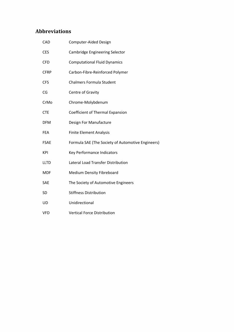
Abbreviations
CAD Computer-Aided Design
CES Cambridge Engineering Selector
CFD Computational Fluid Dynamics
CFRP Carbon-Fibre-Reinforced Polymer
CFS Chalmers Formula Student
CG Centre of Gravity
CrMo Chrome-Molybdenum
CTE Coefficient of Thermal Expansion
DFM Design For Manufacture
FEA Finite Element Analysis
FSAE Formula SAE (The Society of Automotive Engineers)
KPI Key Performance Indicators
LLTD Lateral Load Transfer Distribution
MDF Medium Density Fibreboard
SAE The Society of Automotive Engineers
SD Stiffness Distribution
UD Unidirectional
VFD Vertical Force Distribution
1
1. Introduction Formula Student is an established student engineering, motorsport competition. Teams design and construct a formula-style racing car, adhering to stringent rules and regulations. The cars are then evaluated, through static and dynamic events, with points awarded for parameters of cost, presentation, design, acceleration, skid-pad performance, sprint, endurance and economy.
1.1 Background The chassis is inherently important, as it is the frame, the internal structure that supports all the components and occupants of a race car, preferably in a well-balanced and effective manner. Rigidity in bending and torsion, efficient load absorption and low weight are key to strong chassis performance. [Costin & Phipps 1966]
Space frame and monocoque are currently the preferred chassis types for Formula Student race cars. A space frame chassis involves the assembly of components onto a skeleton-like structure of steel rods. The body provides minimal structural support. Monocoque chassis, however, adapt a unibody approach, where the body is also the structure.
Today, weight and stiffness are perhaps the most important chassis design concerns. New materials are being experimented with and carbon fibre reinforced polymers are rapidly becoming a preferred option, thanks to their inherently strong stiffness, tensile properties and low weight.
1.2 Problem Definition At Chalmers Formula Student (CFS), point analysis has revealed that weight has been detrimental for fuel consumption and dynamic performance. To counter this and still meet the high chassis strength and rigidity targets, CFS will return to using a hybrid composite chassis for the 2013 car.
CFS however, does not have as much experience of composite chassis as they have of space frames. The only composite chassis made by CFS was made in 2006. Back then, several design choices and decisions were based on assumptions due to lack of experience. Ideally these choices should be supported by facts and data. The designers from the latest years of CFS have also expressed difficulty in knowing which of the available chassis design regulations to follow.
1.3 Purpose and Aim The project aims to provide the Formula Student race car of coming years with useful information concerning materials, key performance indicators, the design process and guidelines for efficient chassis design.
To design a chassis that improves the overall dynamic performance of the car it is important to understand what parameters that affect the performance. Key load cases that the chassis will experience are to be determined and studied to understand how they impact chassis performance. A CAD-model will also be created to simulate the most important load cases and to gain knowledge about analysis of composite materials.
The two main chassis design types that will be analysed in this paper are the more traditional tubular space frame and the more modern carbon fibre monocoque. A third variant, which is a combination of both of these, will also be considered but not extensively studied. As carbon fibre offers a lightweight construction and since many of the top teams are using monocoque solutions, more focus will be put into the analysis of carbon fibre
2
monocoque alternatives. The aim is to arrive at the advantages and disadvantages of the different design options, with respect to the found key performance indicators while taking the manufacturability into account. This knowledge will then be compiled into recommendations on how to design a Formula Student chassis.
1.4 Project Boundaries The project will focus on optimizing the chassis performance of a Formula Student race car. To limit the scope of the project, some boundaries will be established. These boundaries are defined to ensure that the paper stays focused on concerns relevant to the problem definition.
No physical prototype of a chassis will be built. Creating a physical prototype is a complex and expensive process that would consume too much time and effort for the group. Instead, focus will lie on improving part solutions, finding key design shapes and establishing design process guidelines. The analysis on space frame tubular chassis will be made on the CFS12 CAD-model to get a reference to the carbon composite model.
For modelling and simulation the computer software ANSYS and CATIA V5 will be used. A static analysis will be done on a simplified model of the chassis to exemplify the significance of chassis rigidity. Dynamic analysis is considered too complex for the scope of the project. Minor analyses considering aerodynamics will be made to establish a general knowledge of aerodynamic properties of a chassis.
1.5 Formulation of Objectives In summary, the purpose of this project can be stated as follows:
“By the 1st of June 2013, through research and finite element analysis, we will deliver a professional report to Chalmers Formula Student, which clearly identifies and explains the key performance indicators of a race car chassis, to help improve the overall performance of the 2014 CFS car.”
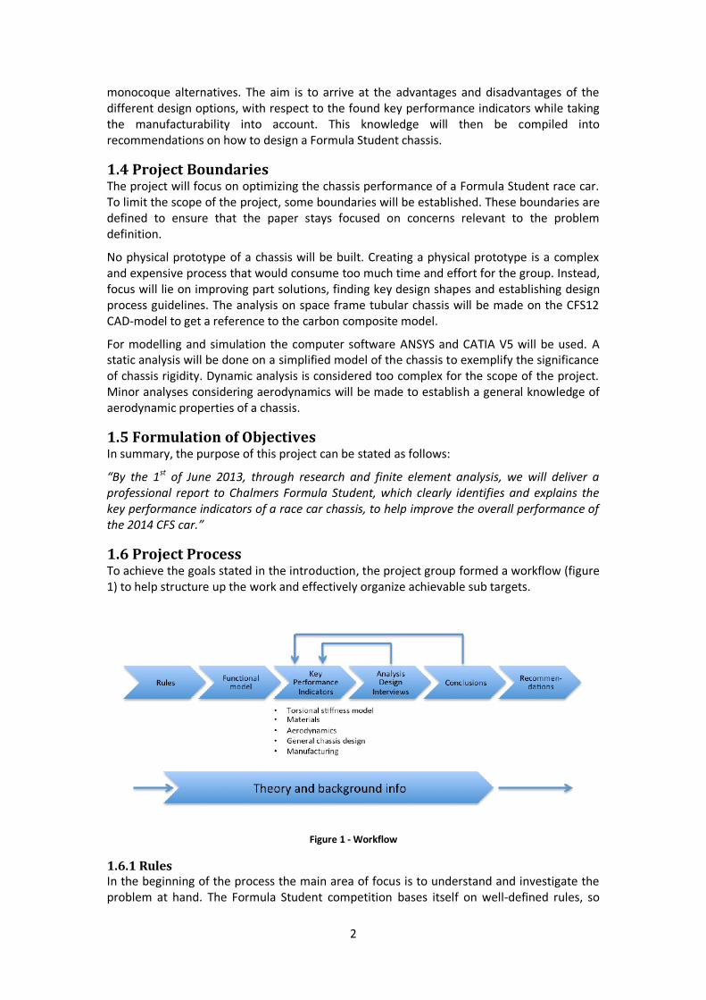
1.6 Project Process To achieve the goals stated in the introduction, the project group formed a workflow (figure 1) to help structure up the work and effectively organize achievable sub targets.
Figure 1 - Workflow
1.6.1 Rules In the beginning of the process the main area of focus is to understand and investigate the problem at hand. The Formula Student competition bases itself on well-defined rules, so
3
initially reading and understanding them is a priority. Simultaneously a background information search is initiated with focus on different chassis solutions and competitor teams.
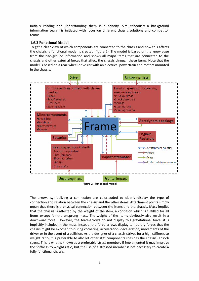
1.6.2 Functional Model To get a clear view of which components are connected to the chassis and how this affects the chassis, a functional model is created (figure 2). The model is based on the knowledge from the background information and shows all major items that are connected to the chassis and other external forces that affect the chassis through these items. Note that the model is based on a rear-wheel drive car with an electrical powertrain and motors mounted in the chassis.
Figure 2 - Functional model
The arrows symbolizing a connection are color-coded to clearly display the type of connection and relation between the chassis and the other items. Attachment points simply mean that there is a physical connection between the items and the chassis. Mass implies that the chassis is affected by the weight of the item, a condition which is fulfilled for all items except for the unsprung mass. The weight of the items obviously also result in a downward force. However, the force-arrows do not display this gravitational force; it is implicitly included in the mass. Instead, the force-arrows display temporary forces that the chassis might be exposed to during cornering, acceleration, deceleration, movements of the driver or in the event of a collision. As the designer of a chassis strives for a high stiffness to weight ratio, it is preferable to also let other stiff components (besides the chassis) absorb stress. This is what is known as a preferable stress member. If implemented it may improve the stiffness to weight ratio, but the use of a stressed member is not necessary to create a fully functional chassis.
4
1.6.3 Key Performance Indicators A key performance indicator (KPI) is a quantitative or qualitative value of data that evaluates the performance of a product or service. For the product to achieve its performance goals these KPIs must be a central part of the design. KPIs for a racing car can range from low weight or high stiffness to aerodynamic considerations and tire performance. In the case of a Formula Student car chassis there are some KPIs of greater importance than others, and to identify these is important to be able to measure performance during the design process. When certain KPIs are established, analysis and modelling will use them as performance measurement to decide key aspects of the design.
1.6.4 Analysis, Design & Interviews To draw conclusions that lead to useful recommendations, several analyses are conducted, a CAD model of a composite chassis is designed and knowledgeable individuals within CFS are interviewed. The purpose of torsional stiffness is analysed in a static cornering model and computational fluid dynamics software (FLUENT) is used to analyse the key design shapes of a chassis. When general design aspects are determined, it is important to make a wise decision on material choice and manufacturing process. In order to gain knowledge of how composite material acts in a monocoque chassis, a CAD model is designed and then used in the ANSYS and FLUENT analyses. Individuals from CFS are interviewed concerning the design process of a Formula Student car, in order to make use of their experience. Reading of relevant literature and articles throughout the research process also helps directing and implementing the study.
1.6.5 Conclusions and recommendations After the analysis, design and interviews part of the project is done, the next step is to draw deliberated conclusions based on the knowledge gained earlier in the project. These conclusions summarize how different KPIs and design goals are accomplished. A conclusion can for example tell that an assumption made in the KPI part was wrong. By iterating back to the KPI phase of the project the indicator or parameter can be changed to match up and satisfy the conclusion. Sometimes conclusions can be difficult to draw considering the complexity of many problems, but in the end it must be done to reach the final step in the project. As can be seen in the formulation of objectives, the main goal with the project is to deliver a report that will be useful to the CFS team. The report aims to help improve the performance of the team by providing helpful and valuable recommendations.
5
2. Theory To effectively address the problem at hand, it is imperative to gain an in-depth understanding of the different chassis types and their history, materials used, the different load cases and the relevant load paths. Below, different chassis design types and their characteristics are introduced.
2.1 Chassis Design and History Earlier, race cars were constructed on massive lines, a design trait that reflected bridge-building more than performance engineering. Prior to World War II almost all car chassis were of the girder type, a construction of beams, usually I-shaped or Z-shaped.
Mercedes-Benz introduced tubular beams in 1937. In such a chassis, the beams were parallel, from axle to axle and the construction was known as a twin-tube. It remained in vogue for racing cars until the early 1950s, when chassis with space frame principles started appearing with the Lotus Mark Six and Mercedes-Benz 300SL. Space frames continued to become widely used throughout the race car industry and were also implemented in some specialist road cars. [Costin and Phipps 1966]
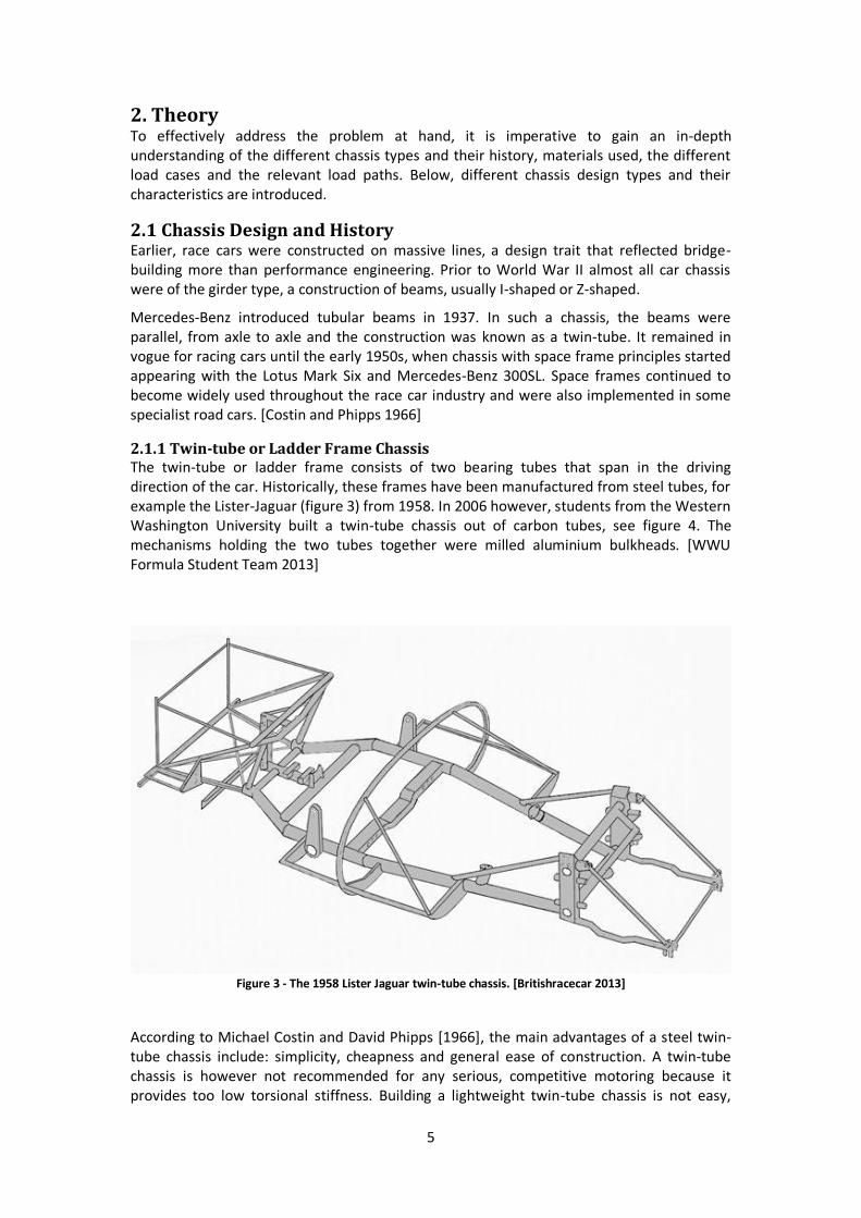
2.1.1 Twin-tube or Ladder Frame Chassis The twin-tube or ladder frame consists of two bearing tubes that span in the driving direction of the car. Historically, these frames have been manufactured from steel tubes, for example the Lister-Jaguar (figure 3) from 1958. In 2006 however, students from the Western Washington University built a twin-tube chassis out of carbon tubes, see figure 4. The mechanisms holding the two tubes together were milled aluminium bulkheads. [WWU Formula Student Team 2013]
Figure 3 - The 1958 Lister Jaguar twin-tube chassis. [Britishracecar 2013]
According to Michael Costin and David Phipps [1966], the main advantages of a steel twin-tube chassis include: simplicity, cheapness and general ease of construction. A twin-tube chassis is however not recommended for any serious, competitive motoring because it provides too low torsional stiffness. Building a lightweight twin-tube chassis is not easy,
6
because all the mounting points need extra sub-frames. These sub-frames rarely increase the torsional stiffness.
Figure 4 - Twin-tube chassis [WWU Formula Student Team 2013]
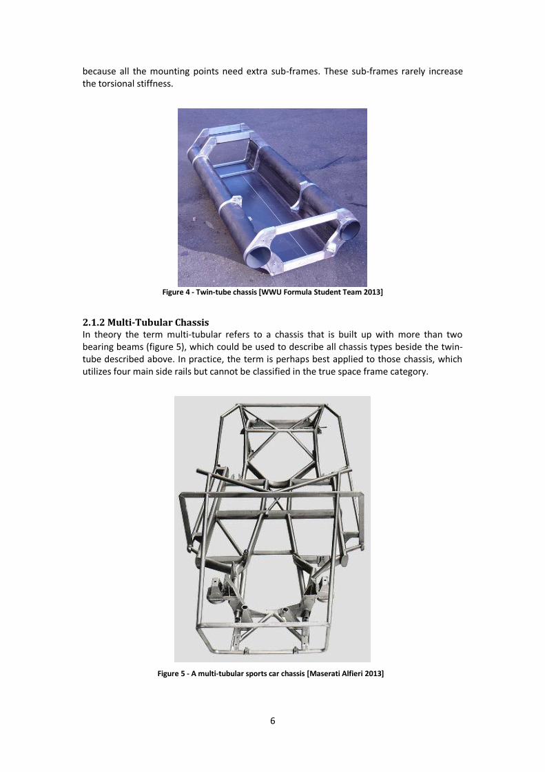
2.1.2 Multi-Tubular Chassis In theory the term multi-tubular refers to a chassis that is built up with more than two bearing beams (figure 5), which could be used to describe all chassis types beside the twin-tube described above. In practice, the term is perhaps best applied to those chassis, which utilizes four main side rails but cannot be classified in the true space frame category.
Figure 5 - A multi-tubular sports car chassis [Maserati Alfieri 2013]
7
Essentially, this chassis offers poor performance, but has proven to be a successful compromise between the twin-tube chassis and the space frame in terms of stiffness and production cost. Often, the frame member diameter, which is the outer diameter of the frame, has to be increased to attain a suitable torsional stiffness. This results in a heavier chassis, in comparison to for example, a space frame that will be introduced in the next paragraph.
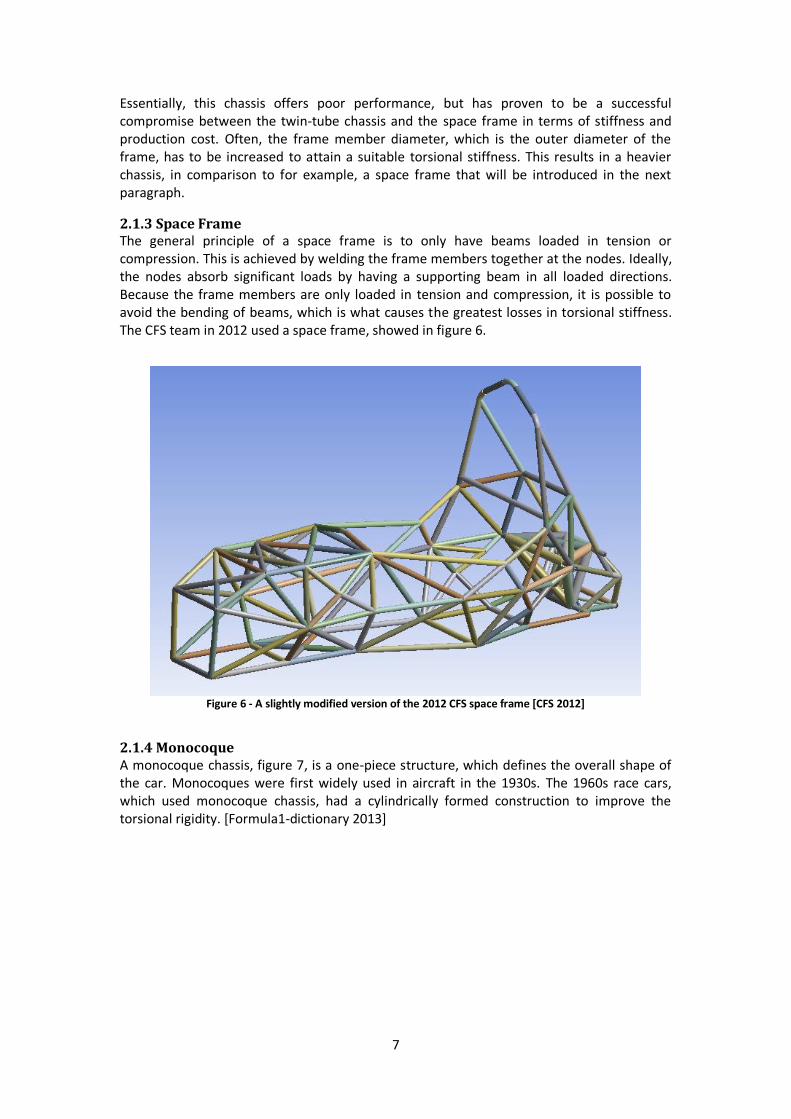
2.1.3 Space Frame The general principle of a space frame is to only have beams loaded in tension or compression. This is achieved by welding the frame members together at the nodes. Ideally, the nodes absorb significant loads by having a supporting beam in all loaded directions. Because the frame members are only loaded in tension and compression, it is possible to avoid the bending of beams, which is what causes the greatest losses in torsional stiffness. The CFS team in 2012 used a space frame, showed in figure 6.
Figure 6 - A slightly modified version of the 2012 CFS space frame [CFS 2012]
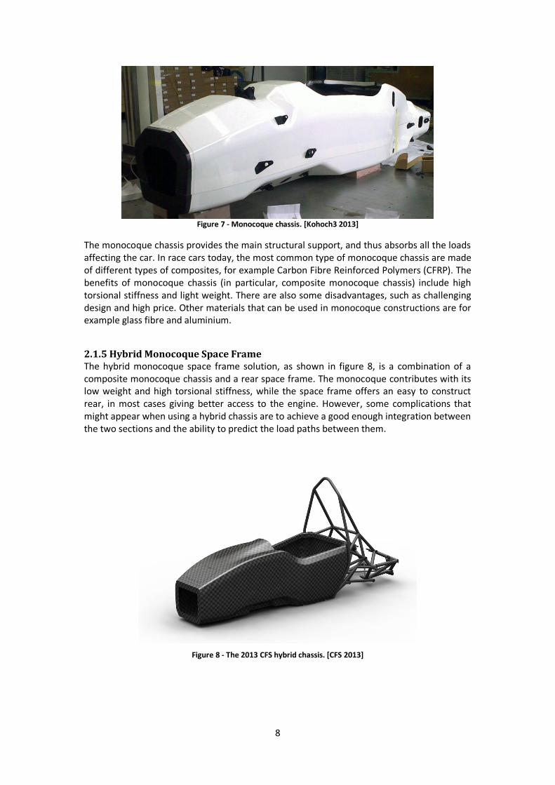
2.1.4 Monocoque A monocoque chassis, figure 7, is a one-piece structure, which defines the overall shape of the car. Monocoques were first widely used in aircraft in the 1930s. The 1960s race cars, which used monocoque chassis, had a cylindrically formed construction to improve the torsional rigidity. [Formula1-dictionary 2013]
8
Figure 7 - Monocoque chassis. [Kohoch3 2013]
The monocoque chassis provides the main structural support, and thus absorbs all the loads affecting the car. In race cars today, the most common type of monocoque chassis are made of different types of composites, for example Carbon Fibre Reinforced Polymers (CFRP). The benefits of monocoque chassis (in particular, composite monocoque chassis) include high torsional stiffness and light weight. There are also some disadvantages, such as challenging design and high price. Other materials that can be used in monocoque constructions are for example glass fibre and aluminium.
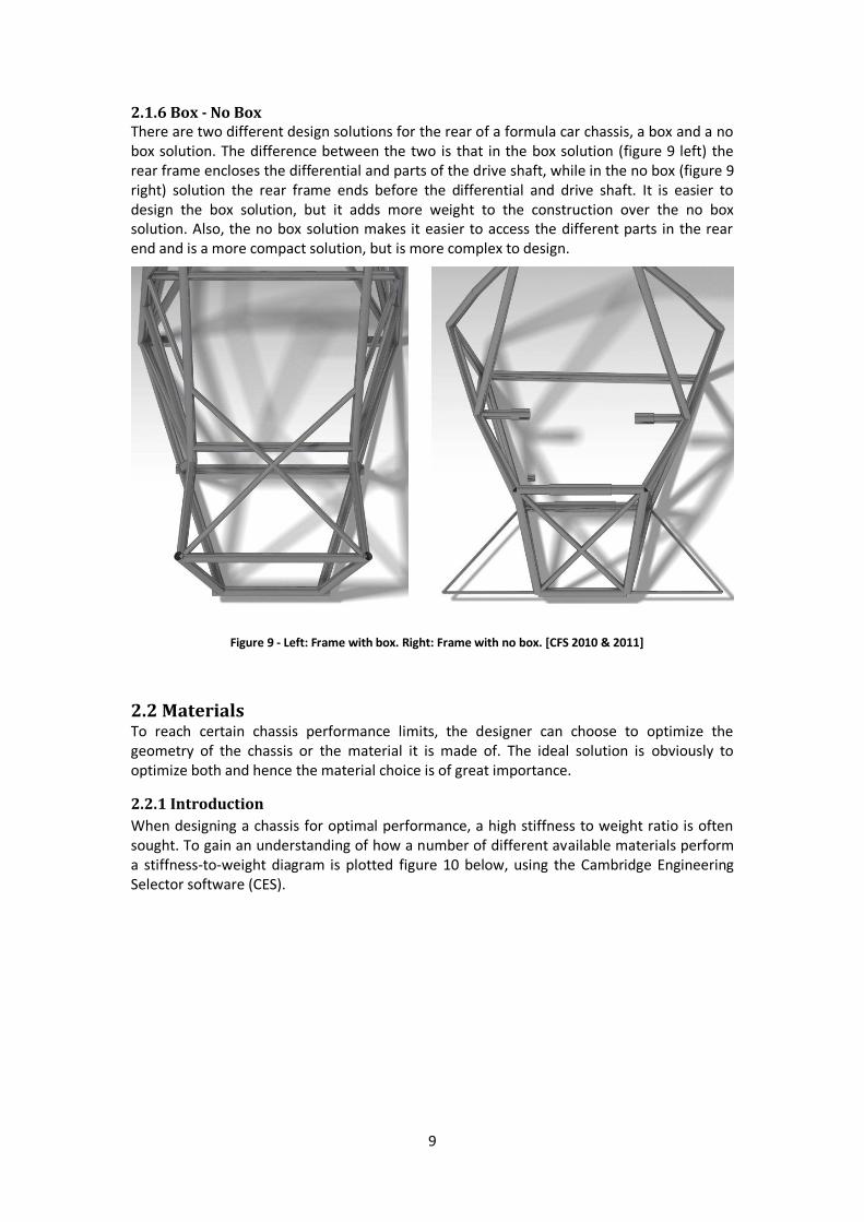
2.1.5 Hybrid Monocoque Space Frame The hybrid monocoque space frame solution, as shown in figure 8, is a combination of a composite monocoque chassis and a rear space frame. The monocoque contributes with its low weight and high torsional stiffness, while the space frame offers an easy to construct rear, in most cases giving better access to the engine. However, some complications that might appear when using a hybrid chassis are to achieve a good enough integration between the two sections and the ability to predict the load paths between them.
Figure 8 - The 2013 CFS hybrid chassis. [CFS 2013]
9
2.1.6 Box - No Box There are two different design solutions for the rear of a formula car chassis, a box and a no box solution. The difference between the two is that in the box solution (figure 9 left) the rear frame encloses the differential and parts of the drive shaft, while in the no box (figure 9 right) solution the rear frame ends before the differential and drive shaft. It is easier to design the box solution, but it adds more weight to the construction over the no box solution. Also, the no box solution makes it easier to access the different parts in the rear end and is a more compact solution, but is more complex to design.
2.2 Materials To reach certain chassis performance limits, the designer can choose to optimize the geometry of the chassis or the material it is made of. The ideal solution is obviously to optimize both and hence the material choice is of great importance.
2.2.1 Introduction
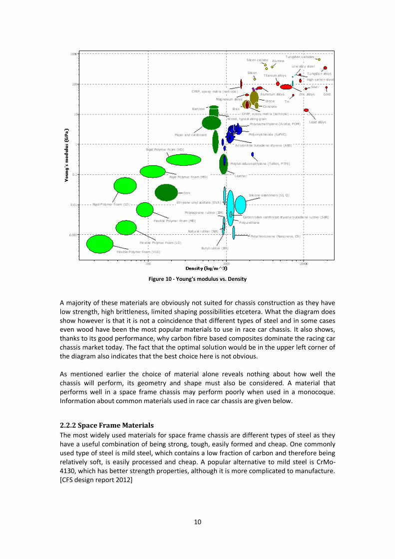
When designing a chassis for optimal performance, a high stiffness to weight ratio is often sought. To gain an understanding of how a number of different available materials perform a stiffness-to-weight diagram is plotted figure 10 below, using the Cambridge Engineering Selector software (CES).
Figure 9 - Left: Frame with box. Right: Frame with no box. [CFS 2010 & 2011]
10
Figure 10 - Young's modulus vs. Density
A majority of these materials are obviously not suited for chassis construction as they have low strength, high brittleness, limited shaping possibilities etcetera. What the diagram does show however is that it is not a coincidence that different types of steel and in some cases even wood have been the most popular materials to use in race car chassis. It also shows, thanks to its good performance, why carbon fibre based composites dominate the racing car chassis market today. The fact that the optimal solution would be in the upper left corner of the diagram also indicates that the best choice here is not obvious. As mentioned earlier the choice of material alone reveals nothing about how well the chassis will perform, its geometry and shape must also be considered. A material that performs well in a space frame chassis may perform poorly when used in a monocoque. Information about common materials used in race car chassis are given below.
2.2.2 Space Frame Materials
The most widely used materials for space frame chassis are different types of steel as they have a useful combination of being strong, tough, easily formed and cheap. One commonly used type of steel is mild steel, which contains a low fraction of carbon and therefore being relatively soft, is easily processed and cheap. A popular alternative to mild steel is CrMo-4130, which has better strength properties, although it is more complicated to manufacture. [CFS design report 2012]
11
Some experiments claim chassis performance can be improved even further by using materials with greater strength and lower weight than steel, like CFRP. The usage of CFRP however, results in new difficulties that do not arise with the usage of steel, like the attachment of the bars to the nodes for instance. [Racecar-Engineering 2013-01]
2.2.3 Monocoque Materials
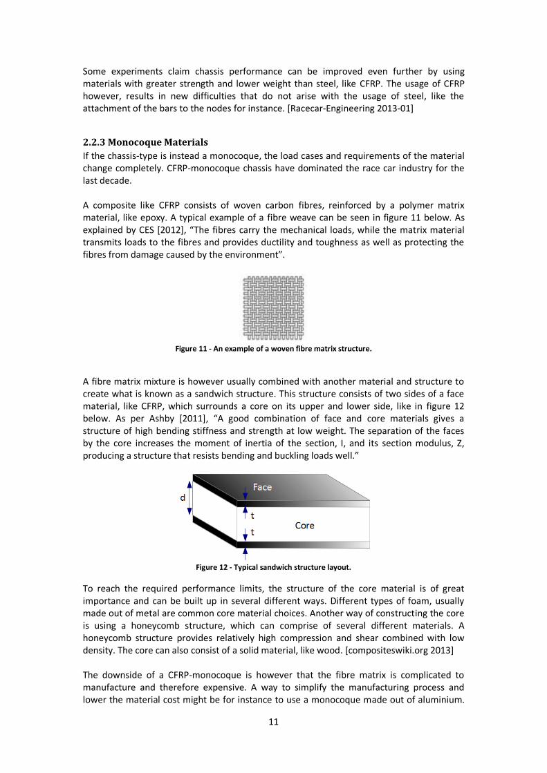
If the chassis-type is instead a monocoque, the load cases and requirements of the material change completely. CFRP-monocoque chassis have dominated the race car industry for the last decade. A composite like CFRP consists of woven carbon fibres, reinforced by a polymer matrix material, like epoxy. A typical example of a fibre weave can be seen in figure 11 below. As explained by CES [2012], “The fibres carry the mechanical loads, while the matrix material transmits loads to the fibres and provides ductility and toughness as well as protecting the fibres from damage caused by the environment”.
Figure 11 - An example of a woven fibre matrix structure.
A fibre matrix mixture is however usually combined with another material and structure to create what is known as a sandwich structure. This structure consists of two sides of a face material, like CFRP, which surrounds a core on its upper and lower side, like in figure 12 below. As per Ashby [2011], “A good combination of face and core materials gives a structure of high bending stiffness and strength at low weight. The separation of the faces by the core increases the moment of inertia of the section, I, and its section modulus, Z, producing a structure that resists bending and buckling loads well.”
To reach the required performance limits, the structure of the core material is of great importance and can be built up in several different ways. Different types of foam, usually made out of metal are common core material choices. Another way of constructing the core is using a honeycomb structure, which can comprise of several different materials. A honeycomb structure provides relatively high compression and shear combined with low density. The core can also consist of a solid material, like wood. [compositeswiki.org 2013] The downside of a CFRP-monocoque is however that the fibre matrix is complicated to manufacture and therefore expensive. A way to simplify the manufacturing process and lower the material cost might be for instance to use a monocoque made out of aluminium.
Figure 12 - Typical sandwich structure layout.
12
The material properties of aluminium however, give the chassis a lower stiffness to weight ratio than that of CFRP. [CES EduPack 2012]
2.3 Chassis Load Cases When designing a chassis it is important to know how it is affected by the different load cases that might occur during driving. These cases will be described further in the following sections.
2.3.1 Global Load Cases The load cases can be divided into global and local cases, where the global focus on load cases affecting the whole chassis whilst the local focus on certain points like mounting points and brackets. The global load cases consist of four cases as described below.
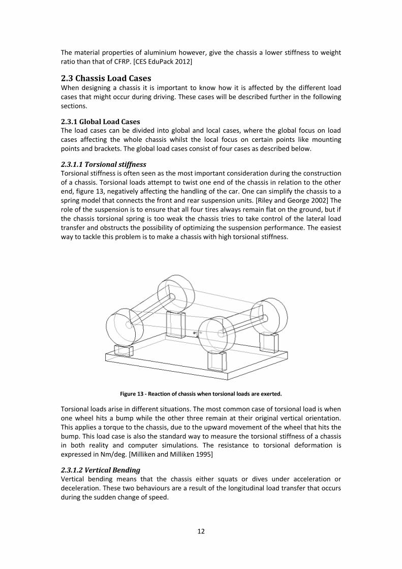
2.3.1.1 Torsional stiffness Torsional stiffness is often seen as the most important consideration during the construction of a chassis. Torsional loads attempt to twist one end of the chassis in relation to the other end, figure 13, negatively affecting the handling of the car. One can simplify the chassis to a spring model that connects the front and rear suspension units. [Riley and George 2002] The role of the suspension is to ensure that all four tires always remain flat on the ground, but if the chassis torsional spring is too weak the chassis tries to take control of the lateral load transfer and obstructs the possibility of optimizing the suspension performance. The easiest way to tackle this problem is to make a chassis with high torsional stiffness.
Figure 13 - Reaction of chassis when torsional loads are exerted.
Torsional loads arise in different situations. The most common case of torsional load is when one wheel hits a bump while the other three remain at their original vertical orientation. This applies a torque to the chassis, due to the upward movement of the wheel that hits the bump. This load case is also the standard way to measure the torsional stiffness of a chassis in both reality and computer simulations. The resistance to torsional deformation is expressed in Nm/deg. [Milliken and Milliken 1995]
2.3.1.2 Vertical Bending Vertical bending means that the chassis either squats or dives under acceleration or deceleration. These two behaviours are a result of the longitudinal load transfer that occurs during the sudden change of speed.
13
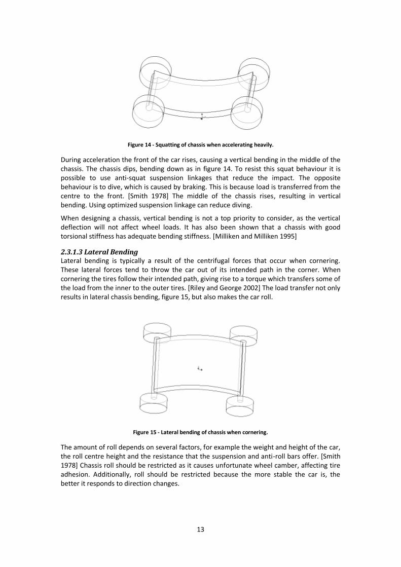
Figure 14 - Squatting of chassis when accelerating heavily.
During acceleration the front of the car rises, causing a vertical bending in the middle of the chassis. The chassis dips, bending down as in figure 14. To resist this squat behaviour it is possible to use anti-squat suspension linkages that reduce the impact. The opposite behaviour is to dive, which is caused by braking. This is because load is transferred from the centre to the front. [Smith 1978] The middle of the chassis rises, resulting in vertical bending. Using optimized suspension linkage can reduce diving.
When designing a chassis, vertical bending is not a top priority to consider, as the vertical deflection will not affect wheel loads. It has also been shown that a chassis with good torsional stiffness has adequate bending stiffness. [Milliken and Milliken 1995]
2.3.1.3 Lateral Bending Lateral bending is typically a result of the centrifugal forces that occur when cornering. These lateral forces tend to throw the car out of its intended path in the corner. When cornering the tires follow their intended path, giving rise to a torque which transfers some of the load from the inner to the outer tires. [Riley and George 2002] The load transfer not only results in lateral chassis bending, figure 15, but also makes the car roll.
Figure 15 - Lateral bending of chassis when cornering.
The amount of roll depends on several factors, for example the weight and height of the car, the roll centre height and the resistance that the suspension and anti-roll bars offer. [Smith 1978] Chassis roll should be restricted as it causes unfortunate wheel camber, affecting tire adhesion. Additionally, roll should be restricted because the more stable the car is, the better it responds to direction changes.
14
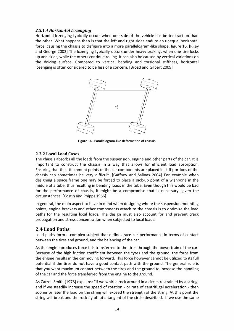
2.3.1.4 Horizontal Lozenging Horizontal lozenging typically occurs when one side of the vehicle has better traction than the other. What happens then is that the left and right sides endure an unequal horizontal force, causing the chassis to disfigure into a more parallelogram-like shape, figure 16. [Riley and George 2002] The lozenging typically occurs under heavy braking, when one tire locks up and skids, while the others continue rolling. It can also be caused by vertical variations on the driving surface. Compared to vertical bending and torsional stiffness, horizontal lozenging is often considered to be less of a concern. [Broad and Gilbert 2009]
Figure 16 - Parallelogram-like deformation of chassis.
2.3.2 Local Load Cases The chassis absorbs all the loads from the suspension, engine and other parts of the car. It is important to construct the chassis in a way that allows for efficient load absorption. Ensuring that the attachment points of the car components are placed in stiff portions of the chassis can sometimes be very difficult. [Gaffney and Salinas 2004] For example when designing a space frame one may be forced to place a pick-up point of a wishbone in the middle of a tube, thus resulting in bending loads in the tube. Even though this would be bad for the performance of chassis, it might be a compromise that is necessary, given the circumstances. [Costin and Phipps 1966]
In general, the main aspect to have in mind when designing where the suspension mounting points, engine brackets and other components attach to the chassis is to optimize the load paths for the resulting local loads. The design must also account for and prevent crack propagation and stress concentration when subjected to local loads.
2.4 Load Paths Load paths form a complex subject that defines race car performance in terms of contact between the tires and ground, and the balancing of the car.
As the engine produces force it is transferred to the tires through the powertrain of the car. Because of the high friction coefficient between the tyres and the ground, the force from the engine results in the car moving forward. This force however cannot be utilized to its full potential if the tires do not have a good contact path with the ground. The general rule is that you want maximum contact between the tires and the ground to increase the handling of the car and the force transferred from the engine to the ground.
As Carroll Smith [1978] explains: “If we whirl a rock around in a circle, restrained by a string, and if we steadily increase the speed of rotation - or rate of centrifugal acceleration - then sooner or later the load on the string will exceed the strength of the string. At this point the string will break and the rock fly off at a tangent of the circle described. If we use the same
15
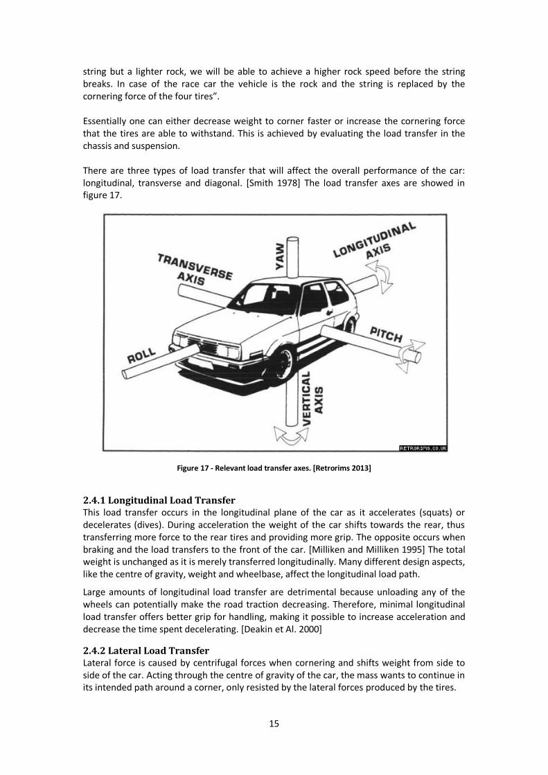
string but a lighter rock, we will be able to achieve a higher rock speed before the string breaks. In case of the race car the vehicle is the rock and the string is replaced by the cornering force of the four tires”. Essentially one can either decrease weight to corner faster or increase the cornering force that the tires are able to withstand. This is achieved by evaluating the load transfer in the chassis and suspension. There are three types of load transfer that will affect the overall performance of the car: longitudinal, transverse and diagonal. [Smith 1978] The load transfer axes are showed in figure 17.
Figure 17 - Relevant load transfer axes. [Retrorims 2013]
2.4.1 Longitudinal Load Transfer This load transfer occurs in the longitudinal plane of the car as it accelerates (squats) or decelerates (dives). During acceleration the weight of the car shifts towards the rear, thus transferring more force to the rear tires and providing more grip. The opposite occurs when braking and the load transfers to the front of the car. [Milliken and Milliken 1995] The total weight is unchanged as it is merely transferred longitudinally. Many different design aspects, like the centre of gravity, weight and wheelbase, affect the longitudinal load path.
Large amounts of longitudinal load transfer are detrimental because unloading any of the wheels can potentially make the road traction decreasing. Therefore, minimal longitudinal load transfer offers better grip for handling, making it possible to increase acceleration and decrease the time spent decelerating. [Deakin et Al. 2000]
2.4.2 Lateral Load Transfer Lateral force is caused by centrifugal forces when cornering and shifts weight from side to side of the car. Acting through the centre of gravity of the car, the mass wants to continue in its intended path around a corner, only resisted by the lateral forces produced by the tires.
16
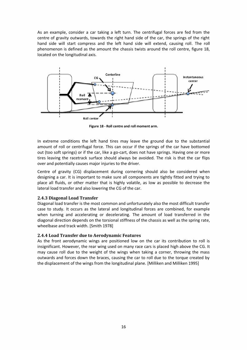
As an example, consider a car taking a left turn. The centrifugal forces are fed from the centre of gravity outwards, towards the right hand side of the car, the springs of the right hand side will start compress and the left hand side will extend, causing roll. The roll phenomenon is defined as the amount the chassis twists around the roll centre, figure 18, located on the longitudinal axis.
Figure 18 - Roll centre and roll moment arm.
In extreme conditions the left hand tires may leave the ground due to the substantial amount of roll or centrifugal force. This can occur if the springs of the car have bottomed out (too soft springs) or if the car, like a go-cart, does not have springs. Having one or more tires leaving the racetrack surface should always be avoided. The risk is that the car flips over and potentially causes major injuries to the driver.
Centre of gravity (CG) displacement during cornering should also be considered when designing a car. It is important to make sure all components are tightly fitted and trying to place all fluids, or other matter that is highly volatile, as low as possible to decrease the lateral load transfer and also lowering the CG of the car.
2.4.3 Diagonal Load Transfer Diagonal load transfer is the most common and unfortunately also the most difficult transfer case to study. It occurs as the lateral and longitudinal forces are combined, for example when turning and accelerating or decelerating. The amount of load transferred in the diagonal direction depends on the torsional stiffness of the chassis as well as the spring rate, wheelbase and track width. [Smith 1978]
2.4.4 Load Transfer due to Aerodynamic Features As the front aerodynamic wings are positioned low on the car its contribution to roll is insignificant. However, the rear wing used on many race cars is placed high above the CG. It may cause roll due to the weight of the wings when taking a corner, throwing the mass outwards and forces down the braces, causing the car to roll due to the torque created by the displacement of the wings from the longitudinal plane. [Milliken and Milliken 1995]
17
3. Research The research section aims to build an in depth understanding of parameters that affect monocoque chassis performance. Different aspects concerning design and manufacture are discussed.
3.1 Key Performance Indicators Key performance indicators are a central part of design and analysis. To identify the most important KPIs research has been conducted. One important indicator of performance that is given the largest amount of attention in the race car chassis community is the torsional rigidity. When comparing longitudinal torsion to vertical and lateral bending, two things can be observed; firstly, the bending cases will not affect the lateral wheel load distribution much, secondly and more importantly, it can be seen that with a correctly designed chassis with high enough torsional stiffness the requirements of bending stiffness is already met. [Milliken and Milliken 1995] On this basis, the main part of the chassis performance section of this project will focus on torsional stiffness.
Stresses are not design determinant on a global scale due to the high tensile strength compared to the Young’s modulus of the materials available. However, local stress concentrations may occur in suspension and engine mounts, as well as in the rocker hard points. Therefore, this has to be monitored closely. These stresses cause local deflections that offset driver input to vehicle reaction. This will also degrade the overall chassis stiffness.
Determining quantitative KPIs for a car chassis is a challenging task that requires deep knowledge and experience of the subject. In the case of chassis stiffness, the final goal is, besides maximizing tire traction, to grant sufficient adjustability of the handling of the car. Thus the stiffness parameter partly comes down to driver preference. Nonetheless one needs to have some specific guidelines when designing the chassis, methods of finding an adequate torsional stiffness will be developed in the next section.
18
3.2 Static Cornering Model/Torsional stiffness model To be able to verify how the chassis behaves while cornering, a static model is developed. The goal of the model is to be able to quantify the design characteristics that create the demand of torsional stiffness. It is commonly said that the chassis should be as stiff as possible, or the stiffer chassis the better performance. One of the problems with a too weak chassis is that it becomes hard to control the lateral load transfer distribution. [Deakin et Al. 2000] A badly balanced car can lead to under- or over steering of the vehicle. The conflicting property that comes with high stiffness is high weight. Therefore, the weight and stiffness of the chassis becomes a matter of compromise.
3.2.1 Method The model considers the centripetal acceleration, the positioning of the centre of gravity on the sprung and unsprang masses, the location of the roll centreline, the front and rear roll stiffness, and the chassis rigidity. With the above properties connected in a static model, the aim is to show how and why previous designers have recommended two different ways of choosing the torsional stiffness to aim for.
Deakin et Al. SAE [2000] states that: “The goal is to determine a chassis stiffness that ensures the vehicle’s handling is sufficiently sensitive to changes in the roll stiffness distribution. A large percentage of the difference in front to rear roll stiffness must therefore result in a difference in front to rear lateral load transfer, for example 80%.”
Milliken and Milliken’s Race Car Vehicle Dynamics [1995] states that the chassis stiffness can be approximately designed to be X times the total suspension roll stiffness, or X times the difference between front and rear suspension stiffness. X is said to be somewhere in the range of 3 - 5 times.
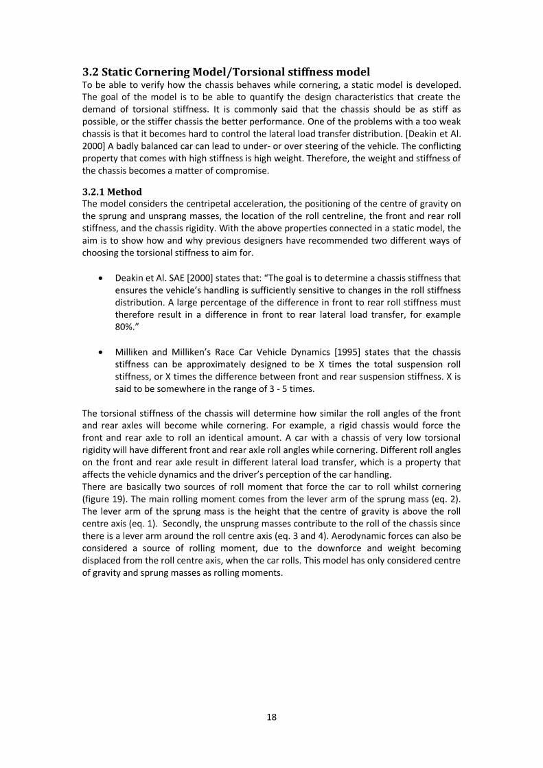
The torsional stiffness of the chassis will determine how similar the roll angles of the front and rear axles will become while cornering. For example, a rigid chassis would force the front and rear axle to roll an identical amount. A car with a chassis of very low torsional rigidity will have different front and rear axle roll angles while cornering. Different roll angles on the front and rear axle result in different lateral load transfer, which is a property that affects the vehicle dynamics and the driver’s perception of the car handling. There are basically two sources of roll moment that force the car to roll whilst cornering (figure 19). The main rolling moment comes from the lever arm of the sprung mass (eq. 2). The lever arm of the sprung mass is the height that the centre of gravity is above the roll centre axis (eq. 1). Secondly, the unsprung masses contribute to the roll of the chassis since there is a lever arm around the roll centre axis (eq. 3 and 4). Aerodynamic forces can also be considered a source of rolling moment, due to the downforce and weight becoming displaced from the roll centre axis, when the car rolls. This model has only considered centre of gravity and sprung masses as rolling moments.
19
Figure 19 - Moments about the roll centreline.
𝑥 = ℎ −
𝑎𝑛 + 𝑏𝑚
𝑎 + 𝑏 (eq. 1)
𝑀𝑠𝑝𝑟𝑢𝑛𝑔 = 𝑎𝑛𝑥𝑚𝑠𝑝𝑟𝑢𝑛𝑔 (eq. 2)
𝑀𝐹𝑟𝑜𝑛𝑡𝑈𝑛𝑆𝑝𝑟𝑢𝑛𝑔 = 𝑎𝑛𝑚𝑓𝑟𝑜𝑛𝑡(𝑟1 − 𝑛) (eq. 3)
𝑀𝑅𝑒𝑎𝑟𝑈𝑛𝑆𝑝𝑟𝑢𝑛𝑔 = 𝑎𝑛𝑚𝑟𝑒𝑎𝑟(𝑟2 − 𝑚) (eq. 4)
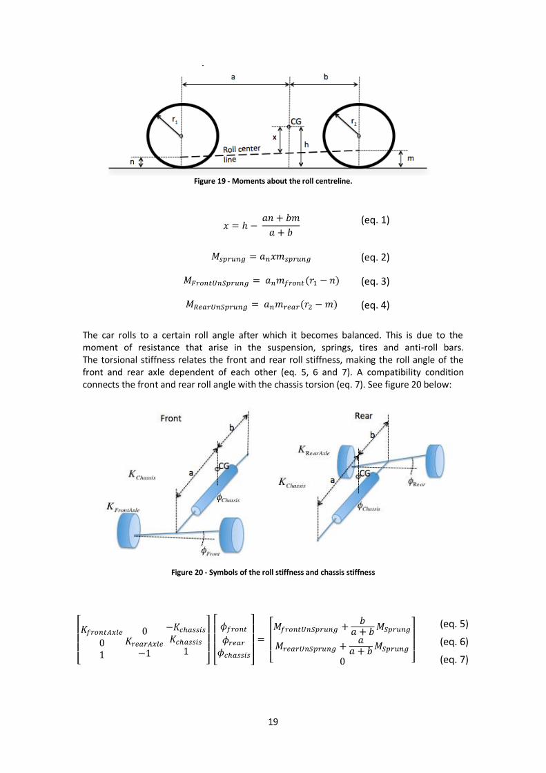
The car rolls to a certain roll angle after which it becomes balanced. This is due to the moment of resistance that arise in the suspension, springs, tires and anti-roll bars. The torsional stiffness relates the front and rear roll stiffness, making the roll angle of the front and rear axle dependent of each other (eq. 5, 6 and 7). A compatibility condition connects the front and rear roll angle with the chassis torsion (eq. 7). See figure 20 below:
Figure 20 - Symbols of the roll stiffness and chassis stiffness
[ 𝐾𝑓𝑟𝑜𝑛𝑡𝐴𝑥𝑙𝑒
01
0𝐾𝑟𝑒𝑎𝑟𝐴𝑥𝑙𝑒
−1
−𝐾𝑐ℎ𝑎𝑠𝑠𝑖𝑠
𝐾𝑐ℎ𝑎𝑠𝑠𝑖𝑠
1 ]
[ 𝜙𝑓𝑟𝑜𝑛𝑡
𝜙𝑟𝑒𝑎𝑟
𝜙𝑐ℎ𝑎𝑠𝑠𝑖𝑠
]
=
[ 𝑀𝑓𝑟𝑜𝑛𝑡𝑈𝑛𝑆𝑝𝑟𝑢𝑛𝑔 +
𝑏𝑎 + 𝑏 𝑀𝑆𝑝𝑟𝑢𝑛𝑔
𝑀𝑟𝑒𝑎𝑟𝑈𝑛𝑆𝑝𝑟𝑢𝑛𝑔 +𝑎
𝑎 + 𝑏 𝑀𝑆𝑝𝑟𝑢𝑛𝑔
0 ]
(eq. 5(eq. 5)
(eq. 6(eq. 6)
(eq. 7(eq. 7)
20
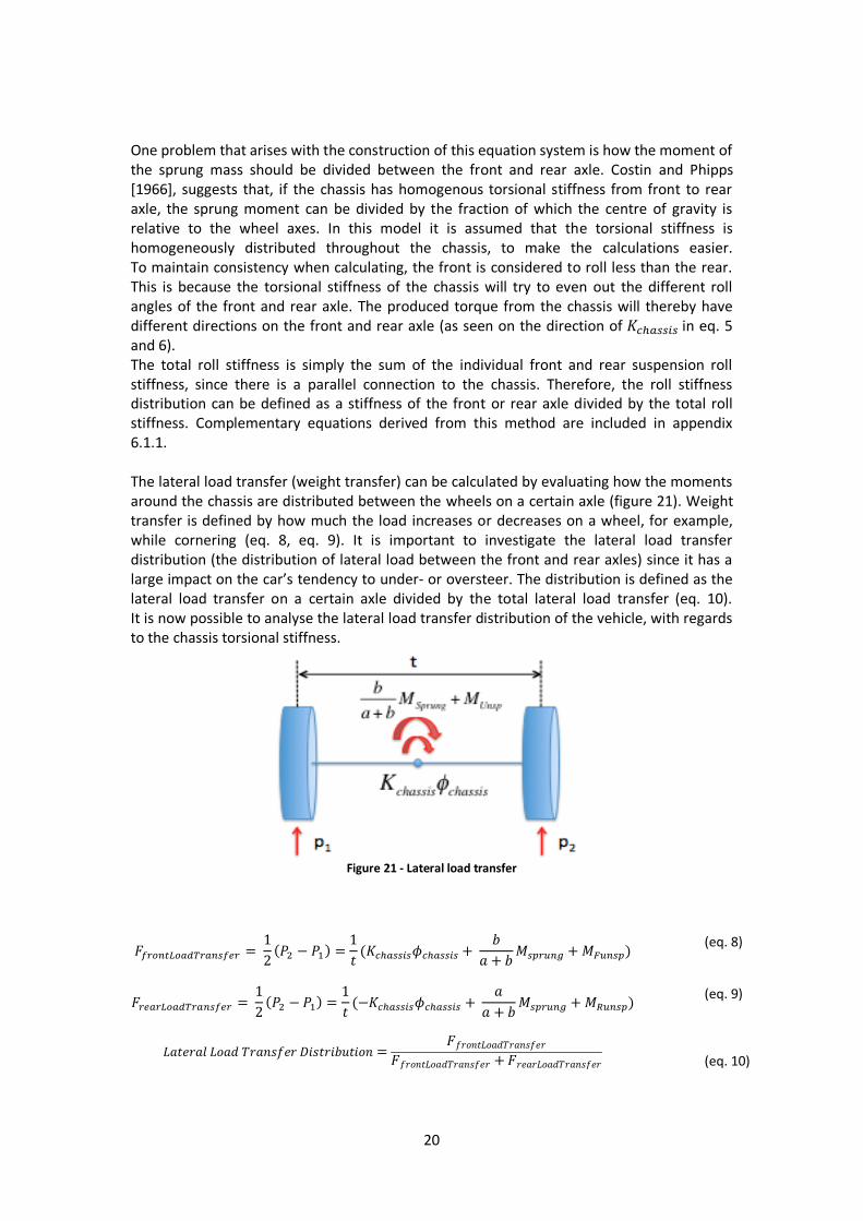
One problem that arises with the construction of this equation system is how the moment of the sprung mass should be divided between the front and rear axle. Costin and Phipps [1966], suggests that, if the chassis has homogenous torsional stiffness from front to rear axle, the sprung moment can be divided by the fraction of which the centre of gravity is relative to the wheel axes. In this model it is assumed that the torsional stiffness is homogeneously distributed throughout the chassis, to make the calculations easier. To maintain consistency when calculating, the front is considered to roll less than the rear. This is because the torsional stiffness of the chassis will try to even out the different roll angles of the front and rear axle. The produced torque from the chassis will thereby have different directions on the front and rear axle (as seen on the direction of 𝐾𝑐ℎ𝑎𝑠𝑠𝑖𝑠 in eq. 5 and 6). The total roll stiffness is simply the sum of the individual front and rear suspension roll stiffness, since there is a parallel connection to the chassis. Therefore, the roll stiffness distribution can be defined as a stiffness of the front or rear axle divided by the total roll stiffness. Complementary equations derived from this method are included in appendix 6.1.1. The lateral load transfer (weight transfer) can be calculated by evaluating how the moments around the chassis are distributed between the wheels on a certain axle (figure 21). Weight transfer is defined by how much the load increases or decreases on a wheel, for example, while cornering (eq. 8, eq. 9). It is important to investigate the lateral load transfer distribution (the distribution of lateral load between the front and rear axles) since it has a large impact on the car’s tendency to under- or oversteer. The distribution is defined as the lateral load transfer on a certain axle divided by the total lateral load transfer (eq. 10). It is now possible to analyse the lateral load transfer distribution of the vehicle, with regards to the chassis torsional stiffness.
Figure 21 - Lateral load transfer
𝐹𝑓𝑟𝑜𝑛𝑡𝐿𝑜𝑎𝑑𝑇𝑟𝑎𝑛𝑠𝑓𝑒𝑟 =
1
2(𝑃2 − 𝑃1) =
1
𝑡(𝐾𝑐ℎ𝑎𝑠𝑠𝑖𝑠𝜙𝑐ℎ𝑎𝑠𝑠𝑖𝑠 +
𝑏
𝑎 + 𝑏𝑀𝑠𝑝𝑟𝑢𝑛𝑔 + 𝑀𝐹𝑢𝑛𝑠𝑝)
(eq. 8)
𝐹𝑟𝑒𝑎𝑟𝐿𝑜𝑎𝑑𝑇𝑟𝑎𝑛𝑠𝑓𝑒𝑟 =
1
2(𝑃2 − 𝑃1) =
1
𝑡(−𝐾𝑐ℎ𝑎𝑠𝑠𝑖𝑠𝜙𝑐ℎ𝑎𝑠𝑠𝑖𝑠 +
𝑎
𝑎 + 𝑏𝑀𝑠𝑝𝑟𝑢𝑛𝑔 + 𝑀𝑅𝑢𝑛𝑠𝑝)
(eq. 9)
𝐿𝑎𝑡𝑒𝑟𝑎𝑙 𝐿𝑜𝑎𝑑 𝑇𝑟𝑎𝑛𝑠𝑓𝑒𝑟 𝐷𝑖𝑠𝑡𝑟𝑖𝑏𝑢𝑡𝑖𝑜𝑛 =
𝐹𝑓𝑟𝑜𝑛𝑡𝐿𝑜𝑎𝑑𝑇𝑟𝑎𝑛𝑠𝑓𝑒𝑟
𝐹𝑓𝑟𝑜𝑛𝑡𝐿𝑜𝑎𝑑𝑇𝑟𝑎𝑛𝑠𝑓𝑒𝑟 + 𝐹𝑟𝑒𝑎𝑟𝐿𝑜𝑎𝑑𝑇𝑟𝑎𝑛𝑠𝑓𝑒𝑟
(eq. 10)
21
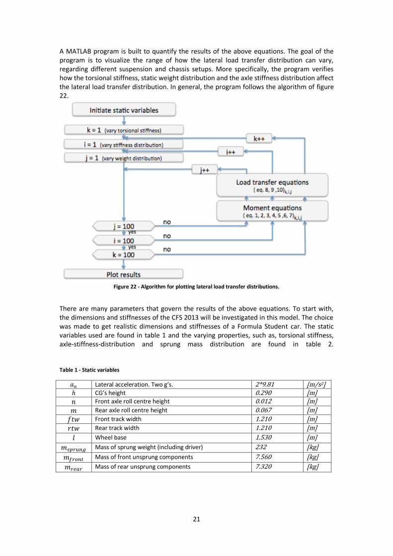
A MATLAB program is built to quantify the results of the above equations. The goal of the program is to visualize the range of how the lateral load transfer distribution can vary, regarding different suspension and chassis setups. More specifically, the program verifies how the torsional stiffness, static weight distribution and the axle stiffness distribution affect the lateral load transfer distribution. In general, the program follows the algorithm of figure 22.
Figure 22 - Algorithm for plotting lateral load transfer distributions.
There are many parameters that govern the results of the above equations. To start with, the dimensions and stiffnesses of the CFS 2013 will be investigated in this model. The choice was made to get realistic dimensions and stiffnesses of a Formula Student car. The static variables used are found in table 1 and the varying properties, such as, torsional stiffness, axle-stiffness-distribution and sprung mass distribution are found in table 2. Table 1 - Static variables
𝑎𝑛 Lateral acceleration. Two g’s. 2*9.81 [m/s2] ℎ CG’s height 0.290 [m]
𝑛 Front axle roll centre height 0.012 [m]
𝑚 Rear axle roll centre height 0.067 [m]
𝑓𝑡𝑤 Front track width 1.210 [m]
𝑟𝑡𝑤 Rear track width 1.210 [m]
𝑙 Wheel base 1.530 [m]
𝑚𝑠𝑝𝑟𝑢𝑛𝑔 Mass of sprung weight (including driver) 232 [kg]
𝑚𝑓𝑟𝑜𝑛𝑡 Mass of front unsprung components 7.560 [kg]
𝑚𝑟𝑒𝑎𝑟 Mass of rear unsprung components 7.320 [kg]
22
Table 2 - Varying variables
𝐾𝑐ℎ𝑎𝑠𝑠𝑖𝑠 Torsional stiffness test range (0 5000] [Nm/deg]
𝐾𝐴𝑥𝑙𝑒𝑅𝑒𝑓 Reference axle stiffness (will later be divided by the fraction of axle-stiffness-distribution).
1400 [Nm/deg]
𝑎 Range of positions of the CG from the front axle (0 1.530) [m]
𝑏 Range of positions of the CG from the rear axle (1.530 0) [m]
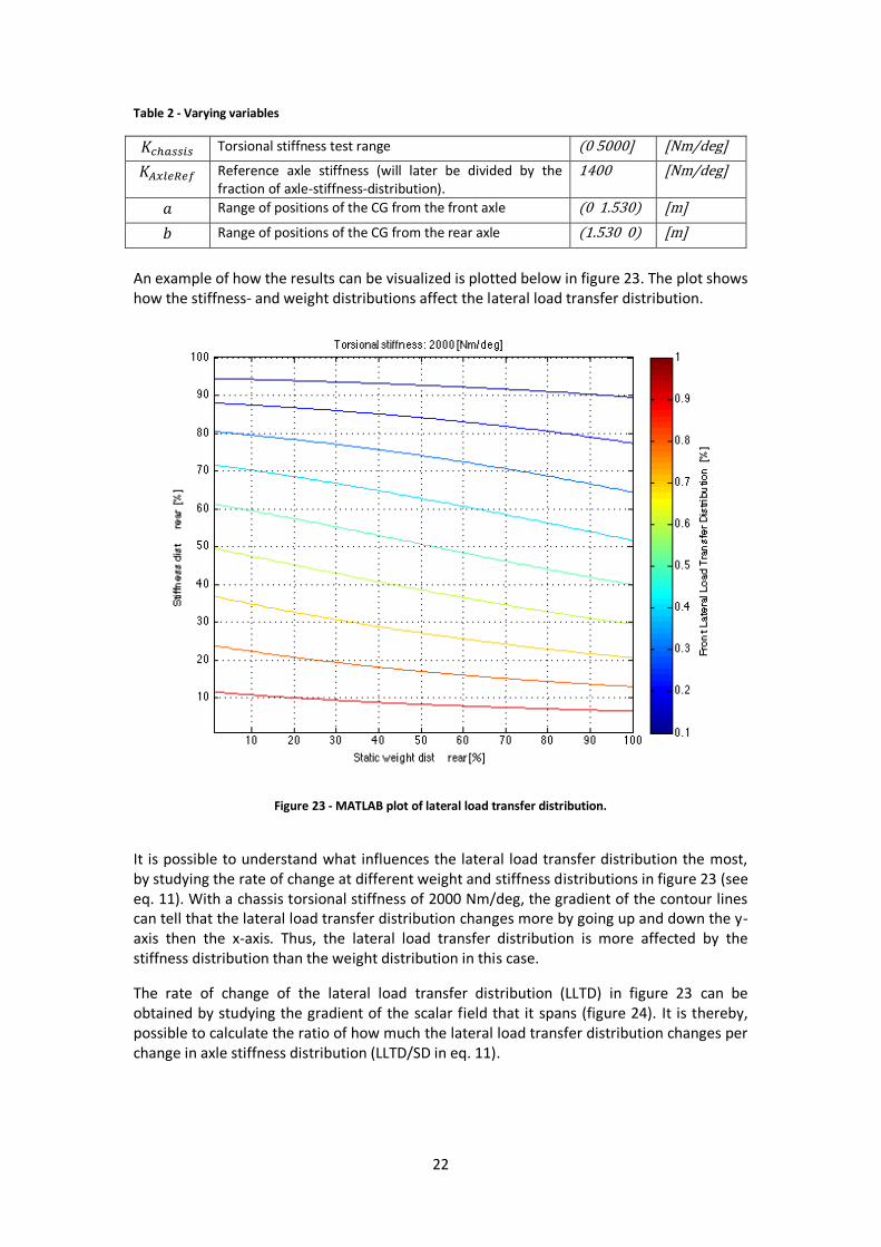
An example of how the results can be visualized is plotted below in figure 23. The plot shows how the stiffness- and weight distributions affect the lateral load transfer distribution.
Figure 23 - MATLAB plot of lateral load transfer distribution.
It is possible to understand what influences the lateral load transfer distribution the most, by studying the rate of change at different weight and stiffness distributions in figure 23 (see eq. 11). With a chassis torsional stiffness of 2000 Nm/deg, the gradient of the contour lines can tell that the lateral load transfer distribution changes more by going up and down the y-axis then the x-axis. Thus, the lateral load transfer distribution is more affected by the stiffness distribution than the weight distribution in this case.
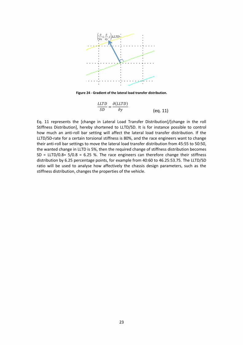
The rate of change of the lateral load transfer distribution (LLTD) in figure 23 can be obtained by studying the gradient of the scalar field that it spans (figure 24). It is thereby, possible to calculate the ratio of how much the lateral load transfer distribution changes per change in axle stiffness distribution (LLTD/SD in eq. 11).
23
Figure 24 - Gradient of the lateral load transfer distribution.
𝐿𝐿𝑇𝐷
𝑆𝐷=
𝜕(𝐿𝐿𝑇𝐷)
𝜕𝑦
(eq. 11)
Eq. 11 represents the [change in Lateral Load Transfer Distribution]/[change in the roll Stiffness Distribution], hereby shortened to LLTD/SD. It is for instance possible to control how much an anti-roll bar setting will affect the lateral load transfer distribution. If the LLTD/SD-rate for a certain torsional stiffness is 80%, and the race engineers want to change their anti-roll bar settings to move the lateral load transfer distribution from 45:55 to 50:50, the wanted change in LLTD is 5%, then the required change of stiffness distribution becomes SD = LLTD/0.8= 5/0.8 = 6.25 %. The race engineers can therefore change their stiffness distribution by 6.25 percentage points, for example from 40:60 to 46.25:53.75. The LLTD/SD ratio will be used to analyse how affectively the chassis design parameters, such as the stiffness distribution, changes the properties of the vehicle.
24
3.2.2 Results The static analysis was performed on a range of different design setups. Varying the torsional stiffness has an impact on the vehicle dynamics and the ability to experience changes in the suspension setup. The lateral load transfer distribution has been used as a measurement of how the torsional stiffness affects the vehicle dynamics. However it is not the change in lateral load transfer distribution that is important in itself; it is the drivers preferences and the vehicles ability to under- or oversteer. Therefore, it is important to be able to control how much a change in the roll stiffness distribution that translates into lateral load transfer distribution. The found parameters that have an impact of how much torsional stiffness that is needed are listed below. They will be explained further in this section.
The total roll stiffness
The roll stiffness distribution between the front and rear axle
The static weight distribution between the front and rear axle
The front and rear roll centre axis
Weight distribution of the front and rear unsprung masses
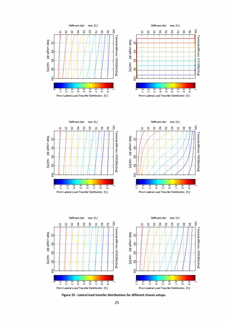
Aerodynamic forces The first two parameters investigated were the roll stiffness distribution and the weight distribution of the front and rear axle. Figure 25 displays six plots with varying the torsional stiffness from 0.01 to 6000 Nm/deg in six steps. The six plots were created using the algorithm of figure 22, which made it possible to plot how the torsional stiffness changes the characteristics of the lateral load transfer distribution. Data from the CFS 2013 car was used as input data throughout the calculations (Table 1 and 2). The total roll stiffness of the car is set to 1400 Nm/deg. A stiffer chassis makes the lateral load transfer distribution change its dependence from the static weight distribution towards the roll stiffness distribution. For example, the first plot of figure 22 shows a car with a torsional stiffness of 0.01 Nm/deg. It is almost only dependent on the static weight distribution, since the contour lines are vertical. As seen in the first plot, varying only the roll stiffness distribution does not change the lateral load transfer distribution for a weak chassis. In the last plot, with a chassis of 6000 Nm/deg, it is possible to see how the torsional stiffness has stabilized the chassis and how the lateral load transfer distribution is more dependent on the roll stiffness distribution. Different weight distributions are effectively absorbed by the chassis stiffness and translated into both the front and rear axle as a load, whilst cornering. With a stiff chassis, the roll stiffness distribution can be approximately set to the wanted lateral load transfer distribution.
25
Figure 25 - Lateral load transfer distributions for different chassis setups.
26
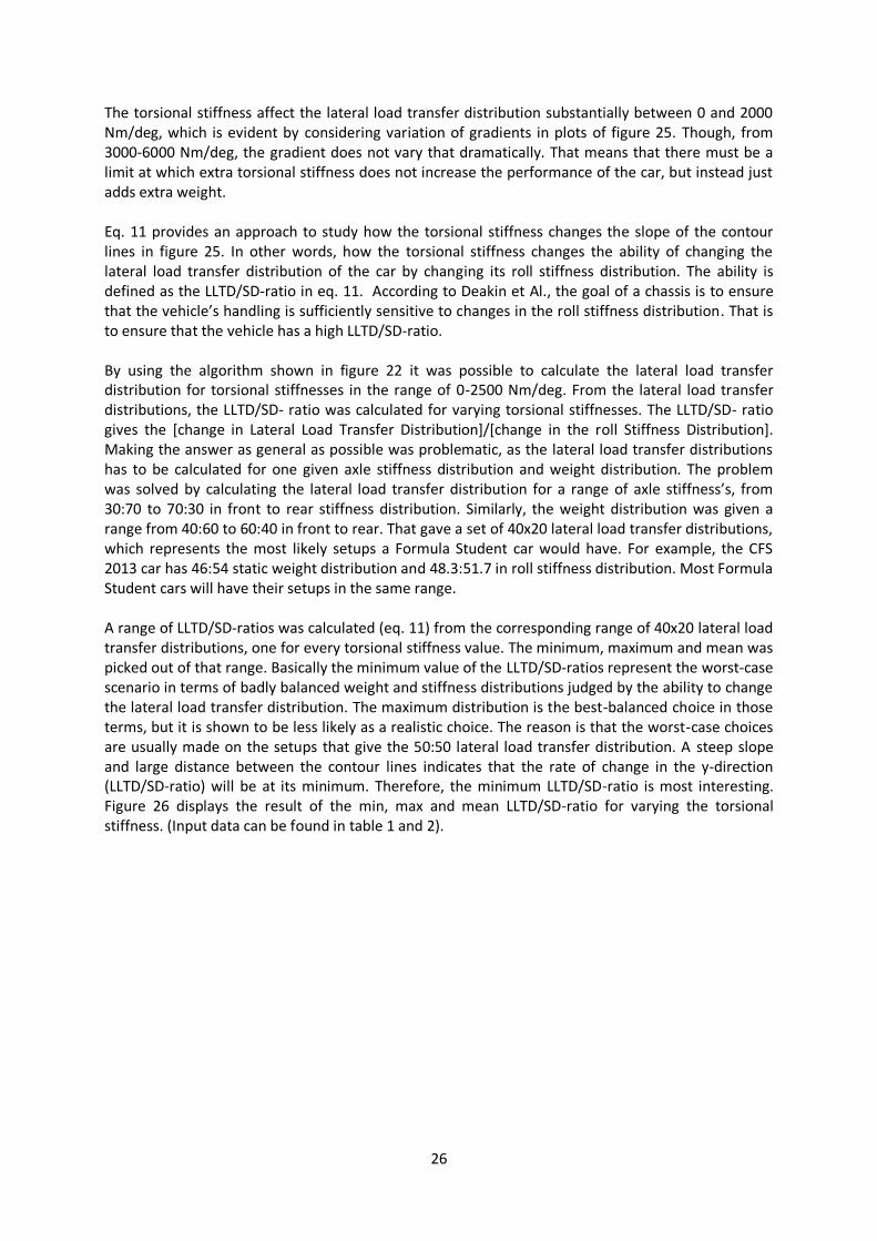
The torsional stiffness affect the lateral load transfer distribution substantially between 0 and 2000 Nm/deg, which is evident by considering variation of gradients in plots of figure 25. Though, from 3000-6000 Nm/deg, the gradient does not vary that dramatically. That means that there must be a limit at which extra torsional stiffness does not increase the performance of the car, but instead just adds extra weight. Eq. 11 provides an approach to study how the torsional stiffness changes the slope of the contour lines in figure 25. In other words, how the torsional stiffness changes the ability of changing the lateral load transfer distribution of the car by changing its roll stiffness distribution. The ability is defined as the LLTD/SD-ratio in eq. 11. According to Deakin et Al., the goal of a chassis is to ensure that the vehicle’s handling is sufficiently sensitive to changes in the roll stiffness distribution. That is to ensure that the vehicle has a high LLTD/SD-ratio. By using the algorithm shown in figure 22 it was possible to calculate the lateral load transfer distribution for torsional stiffnesses in the range of 0-2500 Nm/deg. From the lateral load transfer distributions, the LLTD/SD- ratio was calculated for varying torsional stiffnesses. The LLTD/SD- ratio gives the [change in Lateral Load Transfer Distribution]/[change in the roll Stiffness Distribution]. Making the answer as general as possible was problematic, as the lateral load transfer distributions has to be calculated for one given axle stiffness distribution and weight distribution. The problem was solved by calculating the lateral load transfer distribution for a range of axle stiffness’s, from 30:70 to 70:30 in front to rear stiffness distribution. Similarly, the weight distribution was given a range from 40:60 to 60:40 in front to rear. That gave a set of 40x20 lateral load transfer distributions, which represents the most likely setups a Formula Student car would have. For example, the CFS 2013 car has 46:54 static weight distribution and 48.3:51.7 in roll stiffness distribution. Most Formula Student cars will have their setups in the same range. A range of LLTD/SD-ratios was calculated (eq. 11) from the corresponding range of 40x20 lateral load transfer distributions, one for every torsional stiffness value. The minimum, maximum and mean was picked out of that range. Basically the minimum value of the LLTD/SD-ratios represent the worst-case scenario in terms of badly balanced weight and stiffness distributions judged by the ability to change the lateral load transfer distribution. The maximum distribution is the best-balanced choice in those terms, but it is shown to be less likely as a realistic choice. The reason is that the worst-case choices are usually made on the setups that give the 50:50 lateral load transfer distribution. A steep slope and large distance between the contour lines indicates that the rate of change in the y-direction (LLTD/SD-ratio) will be at its minimum. Therefore, the minimum LLTD/SD-ratio is most interesting. Figure 26 displays the result of the min, max and mean LLTD/SD-ratio for varying the torsional stiffness. (Input data can be found in table 1 and 2).
27
Figure 26 - Min, max and mean LLTD/SD-ratio for varying torsional stiffness. (Eq. 11)
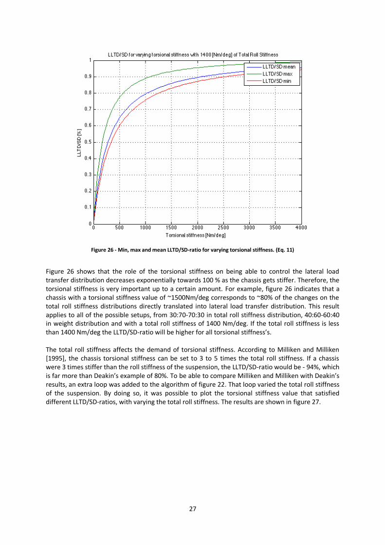
Figure 26 shows that the role of the torsional stiffness on being able to control the lateral load transfer distribution decreases exponentially towards 100 % as the chassis gets stiffer. Therefore, the torsional stiffness is very important up to a certain amount. For example, figure 26 indicates that a chassis with a torsional stiffness value of ~1500Nm/deg corresponds to ~80% of the changes on the total roll stiffness distributions directly translated into lateral load transfer distribution. This result applies to all of the possible setups, from 30:70-70:30 in total roll stiffness distribution, 40:60-60:40 in weight distribution and with a total roll stiffness of 1400 Nm/deg. If the total roll stiffness is less than 1400 Nm/deg the LLTD/SD-ratio will be higher for all torsional stiffness’s. The total roll stiffness affects the demand of torsional stiffness. According to Milliken and Milliken [1995], the chassis torsional stiffness can be set to 3 to 5 times the total roll stiffness. If a chassis were 3 times stiffer than the roll stiffness of the suspension, the LLTD/SD-ratio would be - 94%, which is far more than Deakin’s example of 80%. To be able to compare Milliken and Milliken with Deakin’s results, an extra loop was added to the algorithm of figure 22. That loop varied the total roll stiffness of the suspension. By doing so, it was possible to plot the torsional stiffness value that satisfied different LLTD/SD-ratios, with varying the total roll stiffness. The results are shown in figure 27.
28
Figure 27 - Torsional stiffness satisfying different LLTD/SD-ratios for varying roll stiffness.
The results show that the need of torsional stiffness is linearly proportional to the total roll stiffness of the suspension (in a static analysis). The proportional coefficient depends mainly on the desired LLTD/SD-ratio (eq. 11). Table 3 below presents coefficients that satisfies different LLTD/SD-ratios.
Table 3 - LLTD/SD-ratio comparison of Milliken and Milliken's and Deakin's methods.
𝑇𝑜𝑟𝑠𝑖𝑜𝑛𝑎𝑙 𝑠𝑡𝑖𝑓𝑓𝑛𝑒𝑠𝑠 [𝑁𝑚/𝑑𝑒𝑔]
𝑇𝑜𝑡𝑎𝑙 𝑟𝑜𝑙𝑙 𝑠𝑡𝑖𝑓𝑓𝑛𝑒𝑠𝑠 [𝑁𝑚/𝑑𝑒𝑔] %
𝐿𝐿𝑇𝐷
𝑆𝐷=
[change in Lateral Load Transfer Distribution]
[change in the roll Stiffness Distribution %
0.55 70 %
0.93 80 %
1.22 85 %
1.81 90 %
3.16 95 %
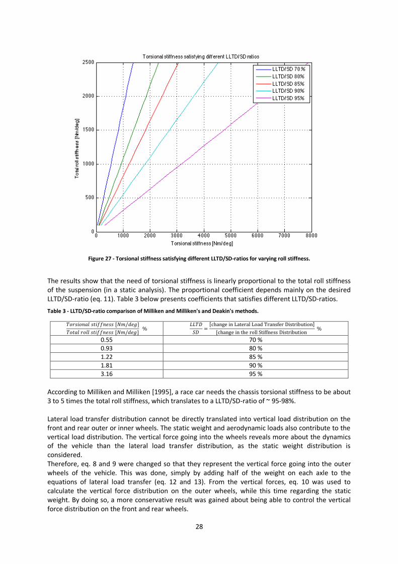
According to Milliken and Milliken [1995], a race car needs the chassis torsional stiffness to be about 3 to 5 times the total roll stiffness, which translates to a LLTD/SD-ratio of ~ 95-98%. Lateral load transfer distribution cannot be directly translated into vertical load distribution on the front and rear outer or inner wheels. The static weight and aerodynamic loads also contribute to the vertical load distribution. The vertical force going into the wheels reveals more about the dynamics of the vehicle than the lateral load transfer distribution, as the static weight distribution is considered. Therefore, eq. 8 and 9 were changed so that they represent the vertical force going into the outer wheels of the vehicle. This was done, simply by adding half of the weight on each axle to the equations of lateral load transfer (eq. 12 and 13). From the vertical forces, eq. 10 was used to calculate the vertical force distribution on the outer wheels, while this time regarding the static weight. By doing so, a more conservative result was gained about being able to control the vertical force distribution on the front and rear wheels.
29
𝐹𝑓𝑉𝐿 =1
𝑡(𝐾𝑐ℎ𝑎𝑠𝑠𝑖𝑠𝜙𝑐ℎ𝑎𝑠𝑠𝑖𝑠 +
𝑏
𝑎+𝑏𝑀𝑠𝑝𝑟𝑢𝑛𝑔 + 𝑀𝐹𝑢𝑛𝑠𝑝) +
𝑎
2(𝑎+𝑏)𝑔𝑚𝑠𝑝𝑟𝑢𝑛𝑔 +
1
2𝑔𝑚𝑓𝑈𝑛𝑠
(eq. 12)
𝐹𝑟𝑉𝐿 =1
𝑡(−𝐾𝑐ℎ𝑎𝑠𝑠𝑖𝑠𝜙𝑐ℎ𝑎𝑠𝑠𝑖𝑠 +
𝑎
𝑎+𝑏𝑀𝑠𝑝𝑟𝑢𝑛𝑔 + 𝑀𝑅𝑢𝑛𝑠𝑝) +
𝑏
2(𝑎+𝑏)𝑔𝑚𝑠𝑝𝑟𝑢𝑛𝑔 +
1
2𝑔𝑚𝑟𝑈𝑛𝑠
(eq. 13)
The result was gained by the same method as above, but the LLTD/SD-ratio was replaced with the VFD/SD-ratio ([change in Vertical Force Distribution]/ [change in Stiffness Distribution]).
Figure 28 - VFD/SD-ratio for varying torsional stiffness, total roll stiffness of 1400 Nm/deg.
Compared to figure 26, figure 28 reveals that it is harder to control the vertical force distribution by changing the roll stiffness distribution. Even with a very stiff chassis of 4000 Nm/deg, the VFD/SD-ratio is ~ 45 %. Having such ratio means that a change in roll stiffness distribution by, for example 10% would give a change in the vertical force distribution by 4.5%. The vertical load distribution of the wheels is harder to control because the static weight distribution plays a large roll on the balance of the car, and on controlling the vertical force distribution.
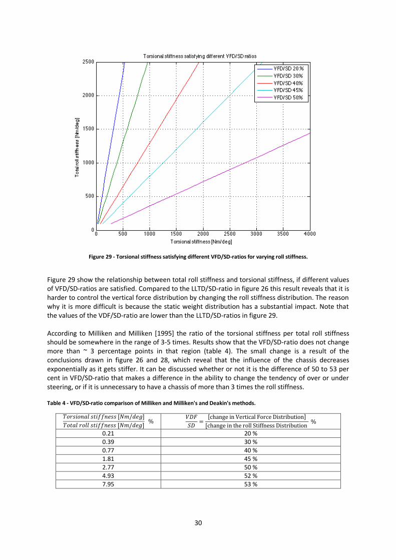
30
Figure 29 - Torsional stiffness satisfying different VFD/SD-ratios for varying roll stiffness.
Figure 29 show the relationship between total roll stiffness and torsional stiffness, if different values of VFD/SD-ratios are satisfied. Compared to the LLTD/SD-ratio in figure 26 this result reveals that it is harder to control the vertical force distribution by changing the roll stiffness distribution. The reason why it is more difficult is because the static weight distribution has a substantial impact. Note that the values of the VDF/SD-ratio are lower than the LLTD/SD-ratios in figure 29. According to Milliken and Milliken [1995] the ratio of the torsional stiffness per total roll stiffness should be somewhere in the range of 3-5 times. Results show that the VFD/SD-ratio does not change more than ~ 3 percentage points in that region (table 4). The small change is a result of the conclusions drawn in figure 26 and 28, which reveal that the influence of the chassis decreases exponentially as it gets stiffer. It can be discussed whether or not it is the difference of 50 to 53 per cent in VFD/SD-ratio that makes a difference in the ability to change the tendency of over or under steering, or if it is unnecessary to have a chassis of more than 3 times the roll stiffness. Table 4 - VFD/SD-ratio comparison of Milliken and Milliken's and Deakin's methods.
𝑇𝑜𝑟𝑠𝑖𝑜𝑛𝑎𝑙 𝑠𝑡𝑖𝑓𝑓𝑛𝑒𝑠𝑠 [𝑁𝑚/𝑑𝑒𝑔]
𝑇𝑜𝑡𝑎𝑙 𝑟𝑜𝑙𝑙 𝑠𝑡𝑖𝑓𝑓𝑛𝑒𝑠𝑠 [𝑁𝑚/𝑑𝑒𝑔] %
𝑉𝐷𝐹
𝑆𝐷=
[change in Vertical Force Distribution]
[change in the roll Stiffness Distribution %
0.21 20 %
0.39 30 %
0.77 40 %
1.81 45 %
2.77 50 %
4.93 52 %
7.95 53 %
31
3.2.3 Criticism of the static cornering model
The method does not consider transient forces form dampers, which can increase the roll stiffness significantly in rapid cornering events. Forces from the dampers are considered to approximately add an equal amount of force due to an even roll of the chassis. It is thereby possible to use the plots in figure 33 and 31 to see the effects.
Having control of the lateral load transfer distribution (which the purpose of a high LLTD/SD ratio is about) is not the same as controlling the ability of the car to over- or understeer. In order to analyse such a case, a transient tire model along with way moment motion equations musts to be analysed, either by hand or in computational software, like CarMaker or Adams.
Aerodynamic down-force has not been considered. It would contribute to the VFD and is important to consider if a full analysis is conducted.
The chassis does not have a homogeneously distributed stiffness, which has been assumed in this model. Varying the distribution of the torsional stiffness does not affect the results of any front or rear axle equations, since it is the total torsional stiffness that matters. It does affect how the sprung mass moment should be divided between the front and rear axle.
The LLTD/SD and VFD/SD-ratios are both derivatives of scalar fields of distributions. It is assumed that the scalar field do not change when changing the stiffness distribution, which is true if the total roll stiffness remains constant. This is usually not the case in reality because an anti-roll bar change may decrease or increase the total roll stiffness by a certain amount and thereby also change the LLTD/SD or VFD/SD-ratio. A calculative test showed that changing the VFD by 10% by only changing the front anti-roll bar causes an error of 2.2% in the VFD/SD-ratio. Because the error is relatively small, and possible to avoid by not changing the total roll stiffness, this was neglected throughout the report.
3.2.4 Conclusions It is vital to have a chassis that provides enough torsional stiffness to the suspension for it to be tuneable. The anti-roll-bars are used for this purpose, while competing. This study has focused on finding ratios of how well the total roll stiffness distribution translates into both lateral load transfer distribution and vertical wheel load distribution. Complementary equations are to be found in appendix 6.1.1. Conclusions that can be drawn are: 1. A stiffer chassis makes the lateral load transfer distribution change its dependence from the
static weight distribution towards the roll stiffness distribution (figure 25).
2. The ability to change the lateral load transfer distribution exponentially approaches 100 %, as the chassis gets stiffer. What determines the rate is mainly the total roll stiffness, but also the weight and stiffness distribution, centre of gravity, roll centre height etc. (figure 26).
3. Results show that the torsional stiffness demand is linearly proportional to the total roll stiffness
of the suspension. The proportional coefficient depends mainly on the wanted LLTD/SD-ratio or VFD/SD-ratio (figure 27 and 28).
4. Milliken and Milliken [1995] states that the torsional stiffness should be about 3-5 times the total
vehicle roll stiffness. It has been shown to be a more conservative rule of thumb when compared to Deakin’s et al [2000]. Deakin states that the vehicles lateral load transfer distribution should be sensitive to changes in the total roll stiffness distribution, for example translated by 80% (the LLTD/SD-ratio). In this study it has been shown that, satisfying 80% of Deakin’s rule of thumb means that the chassis has to be 0.93 times as stiff as the vehicle roll stiffness. Moreover, having a chassis stiffness of 3-5 times the total roll stiffness, will give ~ 95-98% in LLTD/SD-ratio (figure
32
26). Because of the linear behaviour between the roll stiffness and the torsional stiffness demand, it is more practical to say that the chassis should be X times the roll stiffness and include the properties such ratio would provide. For example, if a chassis is designed with torsional stiffness of 1.5 times the roll stiffness, it would give a sensitivity of 88 % LLTD/SD-ratio and 41% VFD/SD-ratio. By this method, it is possible to know how much the anti-roll bars needs to change the roll stiffness distribution to get a desired change of the handling of the vehicle (figure 27 and 29).
5. Results show that it is possible to control the vertical wheel load distribution by changing the roll stiffness distribution, but not as much as it is possible to change the lateral load transfer distribution (figure 29). Even an infinitely stiff chassis will be affected by the static weight distribution, when considering the vertical wheel loads. It is therefore important to mind the positioning of the centre of gravity, as the stiffness distribution hardly controls more than 50% of the vertical wheel loads (figure 29). For example, the VFD/SD-ratio is ~ 48 % for a car with a chassis stiffness of 3000 Nm/deg and a total roll stiffness of 1400 Nm/deg (table 4).
6. Being able to adjust the anti-roll bars with a significant amount could compensate for a weak chassis. If the VFD/SD-ratio is known, it is possible to know by how much the anti-roll bars has to change, to get the desired change in vertical wheel load distribution.
7. Having a chassis stiffness of more than 3 times the roll stiffness of the suspension will add very
few percentage points to the VFD/SD-ratio (table 4). Therefore, if only considering the sensitivity of anti-roll bar changes, it is unnecessary to build a stiffer chassis than about 3 times the total roll stiffness. This result is valid if the stiffness distribution is within the range of 30:70-70:30 and the static weight distribution within 40:60-60:40.
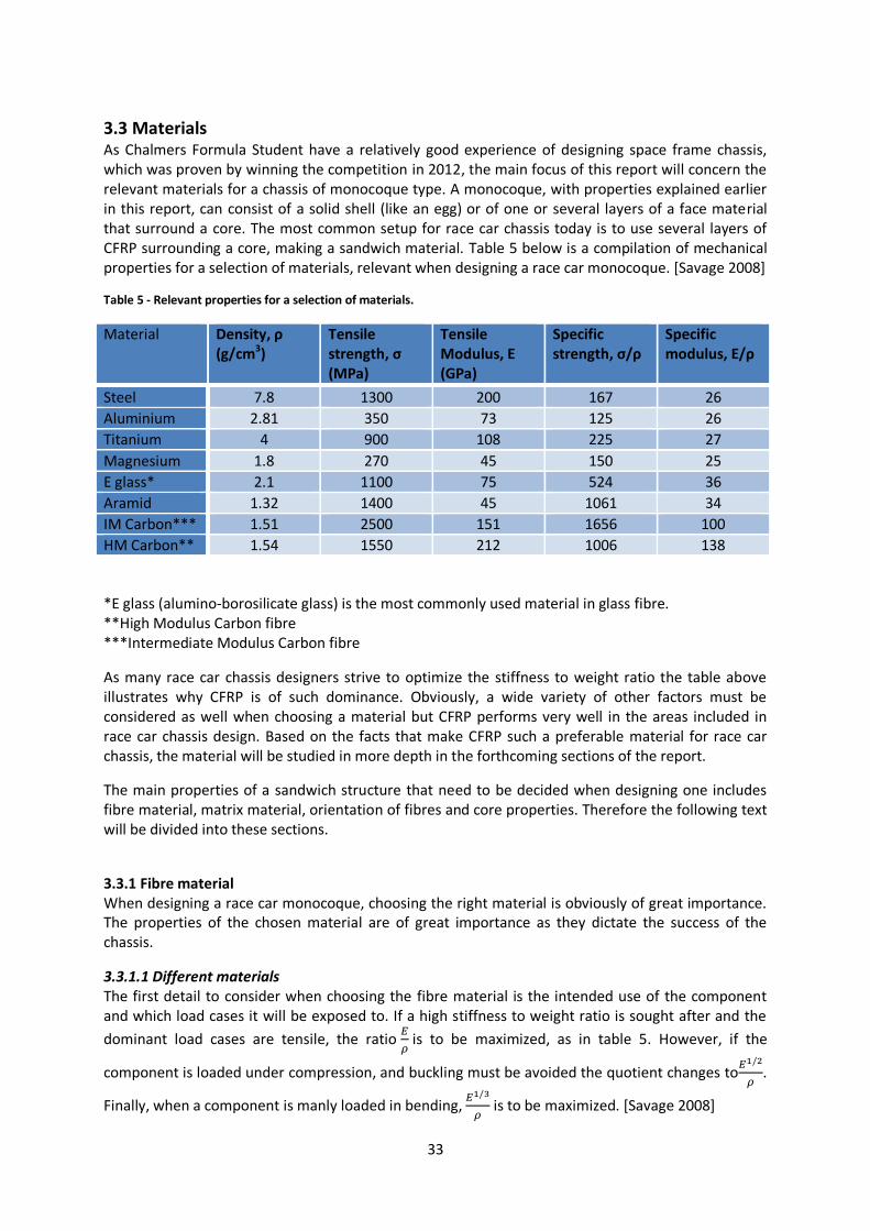
33
3.3 Materials As Chalmers Formula Student have a relatively good experience of designing space frame chassis, which was proven by winning the competition in 2012, the main focus of this report will concern the relevant materials for a chassis of monocoque type. A monocoque, with properties explained earlier in this report, can consist of a solid shell (like an egg) or of one or several layers of a face material that surround a core. The most common setup for race car chassis today is to use several layers of CFRP surrounding a core, making a sandwich material. Table 5 below is a compilation of mechanical properties for a selection of materials, relevant when designing a race car monocoque. [Savage 2008]
Table 5 - Relevant properties for a selection of materials.
Material Density, ρ (g/cm3)
Tensile strength, σ (MPa)
Tensile Modulus, E (GPa)
Specific strength, σ/ρ
Specific modulus, E/ρ
Steel 7.8 1300 200 167 26
Aluminium 2.81 350 73 125 26
Titanium 4 900 108 225 27
Magnesium 1.8 270 45 150 25
E glass* 2.1 1100 75 524 36
Aramid 1.32 1400 45 1061 34
IM Carbon*** 1.51 2500 151 1656 100
HM Carbon** 1.54 1550 212 1006 138
*E glass (alumino-borosilicate glass) is the most commonly used material in glass fibre. **High Modulus Carbon fibre ***Intermediate Modulus Carbon fibre
As many race car chassis designers strive to optimize the stiffness to weight ratio the table above illustrates why CFRP is of such dominance. Obviously, a wide variety of other factors must be considered as well when choosing a material but CFRP performs very well in the areas included in race car chassis design. Based on the facts that make CFRP such a preferable material for race car chassis, the material will be studied in more depth in the forthcoming sections of the report.
The main properties of a sandwich structure that need to be decided when designing one includes fibre material, matrix material, orientation of fibres and core properties. Therefore the following text will be divided into these sections.
3.3.1 Fibre material When designing a race car monocoque, choosing the right material is obviously of great importance. The properties of the chosen material are of great importance as they dictate the success of the chassis.
3.3.1.1 Different materials The first detail to consider when choosing the fibre material is the intended use of the component and which load cases it will be exposed to. If a high stiffness to weight ratio is sought after and the
dominant load cases are tensile, the ratio 𝐸
𝜌 is to be maximized, as in table 5. However, if the
component is loaded under compression, and buckling must be avoided the quotient changes to𝐸1/2
𝜌.
Finally, when a component is manly loaded in bending, 𝐸1/3
𝜌 is to be maximized. [Savage 2008]
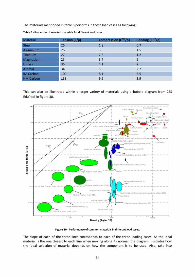
34
The materials mentioned in table 6 performs in these load cases as following:
Table 6 - Properties of selected materials for different load cases.
Material Tension (E/ρ) Compression (E1/2/ρ) Bending (E1/3/ρ)
Steel 26 1.8 0.7
Aluminium 26 3 1.5
Titanium 27 2.6 1.2
Magnesium 25 3.7 2
E glass 36 4.1 2
Aramid 34 5 2.7
IM Carbon 100 8.1 3.5
HM Carbon 138 9.5 3.9
This can also be illustrated within a larger variety of materials using a bubble diagram from CES
EduPack in figure 30.
Figure 30 - Performance of common materials in different load cases.
The slope of each of the three lines corresponds to each of the three loading cases. As the ideal material is the one closest to each line when moving along its normal, the diagram illustrates how the ideal selection of material depends on how the component is to be used. Also, take into
35
consideration that a large majority of these materials are not at all suitable for a race car monocoque to consist of.
As CFRP appears to be the most suitable material for a race car monocoque thus far and is also dominating in the race car industry, CFRP will be the focus of study in the forthcoming parts of this materials section (unless otherwise mentioned).
3.3.1.2 Alternative materials If properties others than those that carbon fibres offer are preferred, a relatively common alternative in the race car industry is to use polymeric fibres instead. The most frequently used polymeric based fibre materials are aramid and zylon.
Aramid is typically known by its trade name, Kevlar. Aramid fibres are suitable for usage where toughness is of great importance as its toughness properties in general are better than those of carbon fibres. Aramid fibres have lower density than carbon fibres and can also be formed into composites using the same techniques. To construct the majority of a chassis out of Aramid fibres is however not recommended as they have much lower compressive strength than carbon fibres. The materials have largely similar properties in tension.
This leads to the fact that aramid fibres are mostly used where good impact and abrasion properties are preferred. A typical area for usage of aramid fibres is underneath the car, preventing possible debris from penetrating the floor.
In the higher levels of auto racing, aramid is however out ruled by the recent developments of higher strength carbon fibres, as they provide both good toughness and compressive strength.
Zylon consists of phenylene and benzobisoxazole, giving it exceptional tensile strength, high modulus and flame resistance. The usage is however relatively limited due to the thermal expansion in the fibre direction at room temperature and poor protection against sunlight and UV-radiation. Thus, the zylon fibres always need to be covered and protected from these factors during usage. Typical usage of zylon fibres in racing cars are as panels in the so called “survival cell” that surround the driver. [formula1-dictionary.net 2013]
Other types of polymeric fibres used in race car chassis, that have excellent strength and low density are polyethylene based continuous filaments with trade names Dyneema and Spectra. As can be understood, there is no such thing as a “wonder material” without downsides. This also holds true for Dyneema and Spectra as their excellent properties only are valid below 90°C.
Since there obviously exists more than a couple of suitable materials to construct a race car chassis with, many of these having different preferable properties with the ability to optimize the design, it is important to not get carried away when trying to find appropriate materials. Savage points out the importance of using as few different materials as possible by claiming that: “this enables a tighter control on logistics and quality control, and allows for a more complete understanding of their properties”.
It is also important to not solely focus on trying to maximize the stiffness to weight ratio as a well performing race car chassis also needs to factor in parameters like a low strain to failure and sufficient damage tolerance. [Savage 2008]
3.3.1.3 Composition types The most relevant types of composition for race car chassis usage are prepreg and infusion. Prepregs are easily formable, weaved or unidirectional carbon fibres, delivered impregnated with the matrix material. The matrix material is of such nature, that in room temperature, it can easily be shaped. When heated up and pressurized, the matrix material solidifies and reaches its final form.
When using infusion, the reinforcement and matrix material (resin) are separated during the shaping process. The fibre weave is shaped to the desired form before being placed in a closed environment.
36
The air around the reinforcement is then removed, creating a vacuum. When the resin is applied, the vacuum causes it to flow through the reinforcement, creating a fibre-reinforced polymer. Lastly, the resin is let to solidify in room temperature and thus the final CFRP component is obtained.
As can be seen, infusion generally requires more work than using prepreg. Infusion is on the other hand usually the cheaper method to use. If the budget permits, prepreg is probably often the preferred method as it usually also results in a higher volume fraction of fibres, giving it a more preferable stiffness to weight ratio. It is also easier to obtain complicated shapes using prepreg.
Savage [2008] summarizes this by saying: “Prepreg ensures that the reinforcement has a precisely defined quantity of fibres in correct location and orientation together with a minimum amount of polymer.”
3.3.2 Matrix material When designing a composite chassis it is important to not compromise on the choice of matrix material. Even the best of fibres will not perform satisfactory if the matrix material does not have the right properties.
The most commonly used matrix materials are thermosetting and thermoplastic polymers. Thermosetting polymers cross-link during the curing process to create a glassy, brittle solid. Examples of thermosetting polymers are polyester and epoxy. Thermoplastic polymers have high molecular weight and provide strength and shape by becoming amorphous or partially crystalline at room temperature. Thermoplastic polymers are for instance polycarbonate and nylon. The race car chassis industry is dominated by thermosetting polymers, which is why these will be the area of focus in the following sections.
CFRP composites consist mainly of three different types of matrix materials: rayon, pitch and polyacrylonitrile, where the latter is the one used most frequently.
As mentioned earlier, the main purpose of the matrix material is to transmit loads to the fibres, protect the fibres from damage and provide ductility and toughness. The ductility and toughness of the matrix depends not only on which material is used, but also on how it is treated during the manufacturing process. The ductility, toughness and modulus of the matrix material are directly linked to the treatment temperature and the applied tension during processing. The strength of polyacrylonitrile based carbon fibres does however reach a peak at a heat treatment temperature of about 1500°C. Because of this limitation other methods have to be used if strength higher than that obtained at maximum heat treatment temperature is sought.
A composite is, as with all materials, limited by how much load it can be exposed to before breaking. Knowing when the composite breaks and how it will break is thus very important. If the composite structure is simplified to a single layer of unidirectional fibres (reinforced by a matrix material), the structure can be loaded in pressure or tension until either the fibres or the matrix material breaks.

37
Figure 31 - Typical failure modes of a fibre and matrix structure
Tension usually leads to either matrix cracking or fibre cracking. A typical failure mode in compression is fibre kinking. All of these failure modes are illustrated in figure 31 above. As with the chain, which is not stronger than its weakest link, having strong fibres can be pointless if a poor matrix material is used, causing it to crack under tension. The ideal solution is therefore to choose a fibre and matrix material which will break simultaneously. [Ashby 2011]
3.3.3 Orientation of fibres As the fibres can be thought of as the backbone of a composite, their orientation is obviously of great importance. Savage explains, “the primary mechanical properties of composites are governed for the most part by the properties of the fibres, their volume fraction, orientation to the applied stress and their “architecture” within the structure”.
The fibres can be positioned in two ways, unidirectional (UD), where all fibres in one layer are in the same direction, or woven to create a weave. Regardless which fibre structured they all consists of tows. An untwisted bundle, called tow, is continuous filaments of carbon fibre, each in size of 5 to 8 μm. [Mazumdar 2002] The number of fibres they contain designates the tow. For example, a 12K tow contains about 12,000 fibres.
UD tapes have the advantage of not being bent, like in a weave, giving them a better translation of fibre properties. UD tapes usually also contains less matrix material than a weave, giving it a higher volume fraction of fibres, and therefore better mechanical properties.
The mechanical properties of UD tapes are however only valid when the load is applied in the same direction as the fibres. If the load is applied at a normal to the fibres, the properties of the composite are basically those of the polymer matrix, with highly limited resistance to stretching. Other advantages for a woven layup also include their performance in complex geometries, lower manufacturing time and better damage resistance.
The layup of a woven composite does however not need to follow the structure of a typical fabric weave, like in figure 32 left, but can be varied in many different ways to optimize the properties of the composite. A composite weave is usually described by a two dimensional coordinate system where the x and y axis respectively are called the weft and warp direction. The most common weaving types used in the composites industry are plain, twill and satin.
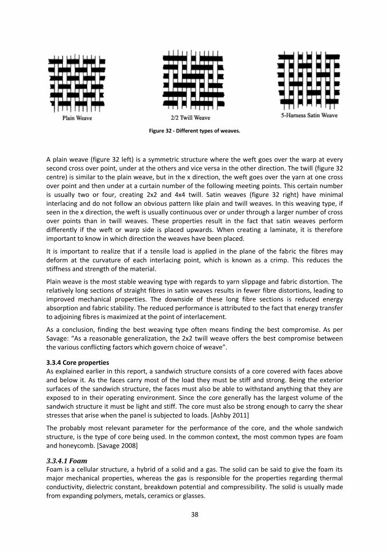
38
A plain weave (figure 32 left) is a symmetric structure where the weft goes over the warp at every second cross over point, under at the others and vice versa in the other direction. The twill (figure 32 centre) is similar to the plain weave, but in the x direction, the weft goes over the yarn at one cross over point and then under at a curtain number of the following meeting points. This certain number is usually two or four, creating 2x2 and 4x4 twill. Satin weaves (figure 32 right) have minimal interlacing and do not follow an obvious pattern like plain and twill weaves. In this weaving type, if seen in the x direction, the weft is usually continuous over or under through a larger number of cross over points than in twill weaves. These properties result in the fact that satin weaves perform differently if the weft or warp side is placed upwards. When creating a laminate, it is therefore important to know in which direction the weaves have been placed.
It is important to realize that if a tensile load is applied in the plane of the fabric the fibres may deform at the curvature of each interlacing point, which is known as a crimp. This reduces the stiffness and strength of the material.
Plain weave is the most stable weaving type with regards to yarn slippage and fabric distortion. The relatively long sections of straight fibres in satin weaves results in fewer fibre distortions, leading to improved mechanical properties. The downside of these long fibre sections is reduced energy absorption and fabric stability. The reduced performance is attributed to the fact that energy transfer to adjoining fibres is maximized at the point of interlacement.
As a conclusion, finding the best weaving type often means finding the best compromise. As per Savage: “As a reasonable generalization, the 2x2 twill weave offers the best compromise between the various conflicting factors which govern choice of weave”.
3.3.4 Core properties As explained earlier in this report, a sandwich structure consists of a core covered with faces above and below it. As the faces carry most of the load they must be stiff and strong. Being the exterior surfaces of the sandwich structure, the faces must also be able to withstand anything that they are exposed to in their operating environment. Since the core generally has the largest volume of the sandwich structure it must be light and stiff. The core must also be strong enough to carry the shear stresses that arise when the panel is subjected to loads. [Ashby 2011]
The probably most relevant parameter for the performance of the core, and the whole sandwich structure, is the type of core being used. In the common context, the most common types are foam and honeycomb. [Savage 2008]
3.3.4.1 Foam Foam is a cellular structure, a hybrid of a solid and a gas. The solid can be said to give the foam its major mechanical properties, whereas the gas is responsible for the properties regarding thermal conductivity, dielectric constant, breakdown potential and compressibility. The solid is usually made from expanding polymers, metals, ceramics or glasses.
Figure 32 - Different types of weaves.
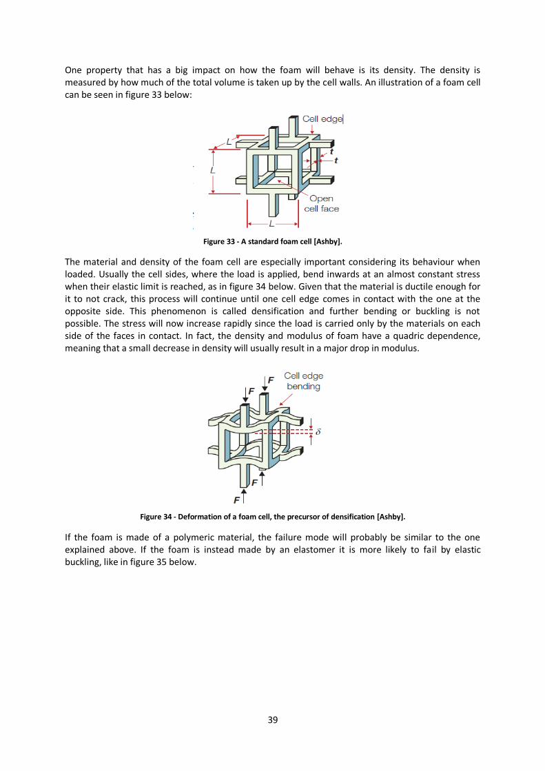
39
One property that has a big impact on how the foam will behave is its density. The density is measured by how much of the total volume is taken up by the cell walls. An illustration of a foam cell can be seen in figure 33 below:
Figure 33 - A standard foam cell [Ashby].
The material and density of the foam cell are especially important considering its behaviour when loaded. Usually the cell sides, where the load is applied, bend inwards at an almost constant stress when their elastic limit is reached, as in figure 34 below. Given that the material is ductile enough for it to not crack, this process will continue until one cell edge comes in contact with the one at the opposite side. This phenomenon is called densification and further bending or buckling is not possible. The stress will now increase rapidly since the load is carried only by the materials on each side of the faces in contact. In fact, the density and modulus of foam have a quadric dependence, meaning that a small decrease in density will usually result in a major drop in modulus.
Figure 34 - Deformation of a foam cell, the precursor of densification [Ashby].
If the foam is made of a polymeric material, the failure mode will probably be similar to the one explained above. If the foam is instead made by an elastomer it is more likely to fail by elastic buckling, like in figure 35 below.
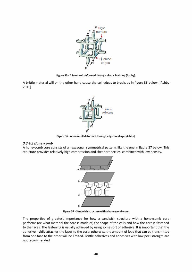
40
Figure 35 - A foam cell deformed through elastic buckling [Ashby].
A brittle material will on the other hand cause the cell edges to break, as in figure 36 below. [Ashby 2011]
Figure 36 - A foam cell deformed through edge breakage [Ashby].
3.3.4.2 Honeycomb A honeycomb core consists of a hexagonal, symmetrical pattern, like the one in figure 37 below. This structure provides relatively high compression and shear properties, combined with low density.
Figure 37 - Sandwich structure with a honeycomb core.
The properties of greatest importance for how a sandwich structure with a honeycomb core performs are what material the core is made of, the shape of the cells and how the core is fastened to the faces. The fastening is usually achieved by using some sort of adhesive. It is important that the adhesive rigidly attaches the faces to the core; otherwise the amount of load that can be transmitted from one face to the other will be limited. Brittle adhesives and adhesives with low peel strength are not recommended.
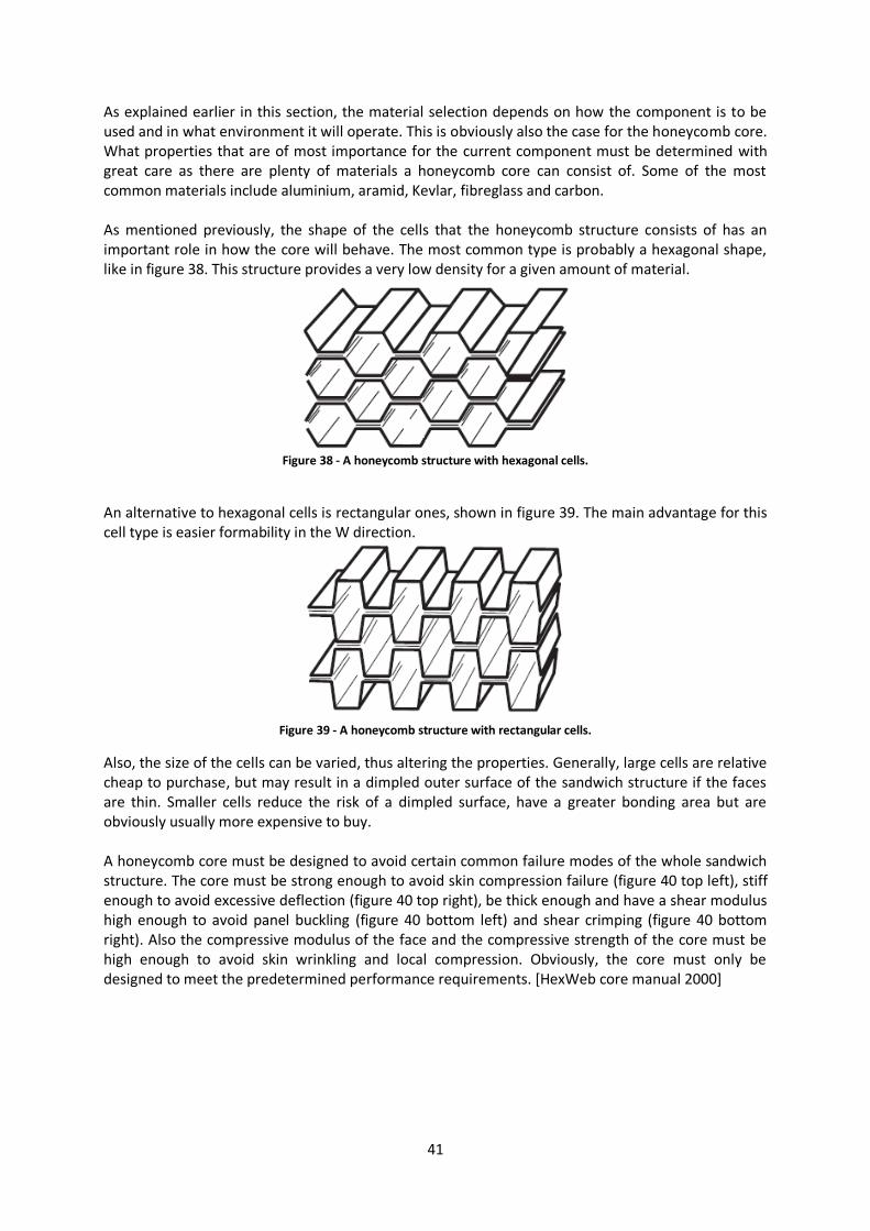
41
As explained earlier in this section, the material selection depends on how the component is to be used and in what environment it will operate. This is obviously also the case for the honeycomb core. What properties that are of most importance for the current component must be determined with great care as there are plenty of materials a honeycomb core can consist of. Some of the most common materials include aluminium, aramid, Kevlar, fibreglass and carbon. As mentioned previously, the shape of the cells that the honeycomb structure consists of has an important role in how the core will behave. The most common type is probably a hexagonal shape, like in figure 38. This structure provides a very low density for a given amount of material.
Figure 38 - A honeycomb structure with hexagonal cells.
An alternative to hexagonal cells is rectangular ones, shown in figure 39. The main advantage for this cell type is easier formability in the W direction.
Figure 39 - A honeycomb structure with rectangular cells.
Also, the size of the cells can be varied, thus altering the properties. Generally, large cells are relative cheap to purchase, but may result in a dimpled outer surface of the sandwich structure if the faces are thin. Smaller cells reduce the risk of a dimpled surface, have a greater bonding area but are obviously usually more expensive to buy. A honeycomb core must be designed to avoid certain common failure modes of the whole sandwich structure. The core must be strong enough to avoid skin compression failure (figure 40 top left), stiff enough to avoid excessive deflection (figure 40 top right), be thick enough and have a shear modulus high enough to avoid panel buckling (figure 40 bottom left) and shear crimping (figure 40 bottom right). Also the compressive modulus of the face and the compressive strength of the core must be high enough to avoid skin wrinkling and local compression. Obviously, the core must only be designed to meet the predetermined performance requirements. [HexWeb core manual 2000]
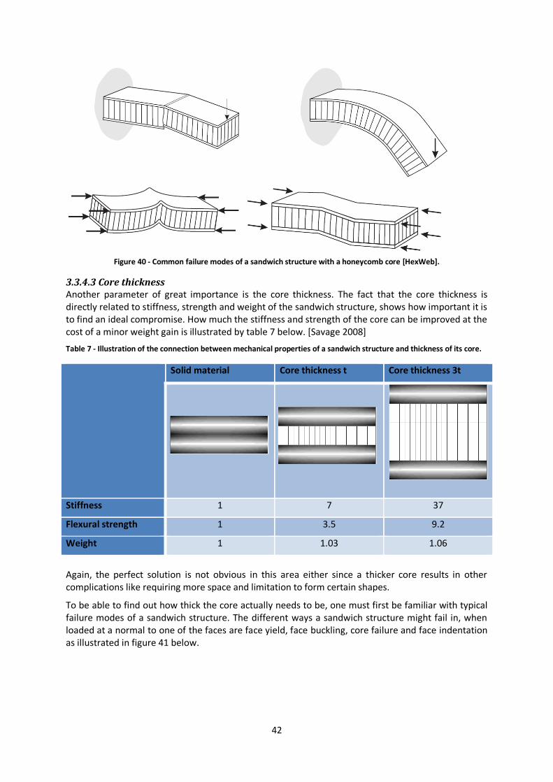
42
Figure 40 - Common failure modes of a sandwich structure with a honeycomb core [HexWeb].
3.3.4.3 Core thickness Another parameter of great importance is the core thickness. The fact that the core thickness is directly related to stiffness, strength and weight of the sandwich structure, shows how important it is to find an ideal compromise. How much the stiffness and strength of the core can be improved at the cost of a minor weight gain is illustrated by table 7 below. [Savage 2008]
Table 7 - Illustration of the connection between mechanical properties of a sandwich structure and thickness of its core.
Solid material Core thickness t Core thickness 3t
Stiffness 1 7 37
Flexural strength 1 3.5 9.2
Weight 1 1.03 1.06
Again, the perfect solution is not obvious in this area either since a thicker core results in other complications like requiring more space and limitation to form certain shapes.
To be able to find out how thick the core actually needs to be, one must first be familiar with typical failure modes of a sandwich structure. The different ways a sandwich structure might fail in, when loaded at a normal to one of the faces are face yield, face buckling, core failure and face indentation as illustrated in figure 41 below.
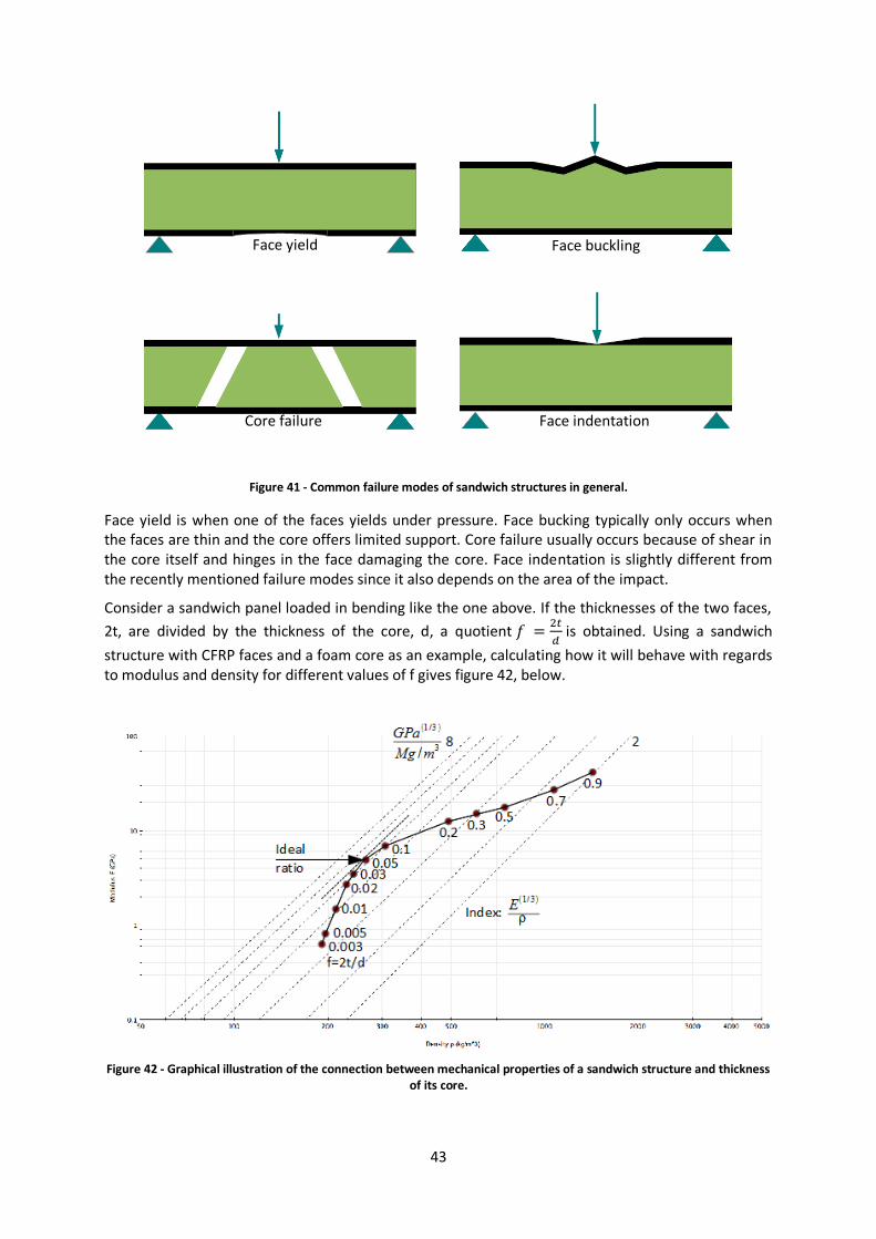
43
Figure 41 - Common failure modes of sandwich structures in general.
Face yield is when one of the faces yields under pressure. Face bucking typically only occurs when the faces are thin and the core offers limited support. Core failure usually occurs because of shear in the core itself and hinges in the face damaging the core. Face indentation is slightly different from the recently mentioned failure modes since it also depends on the area of the impact.
Consider a sandwich panel loaded in bending like the one above. If the thicknesses of the two faces,
2t, are divided by the thickness of the core, d, a quotient 𝑓 =2𝑡
𝑑 is obtained. Using a sandwich
structure with CFRP faces and a foam core as an example, calculating how it will behave with regards to modulus and density for different values of f gives figure 42, below.
Figure 42 - Graphical illustration of the connection between mechanical properties of a sandwich structure and thickness of its core.
Face yield Face buckling
Core failure Face indentation
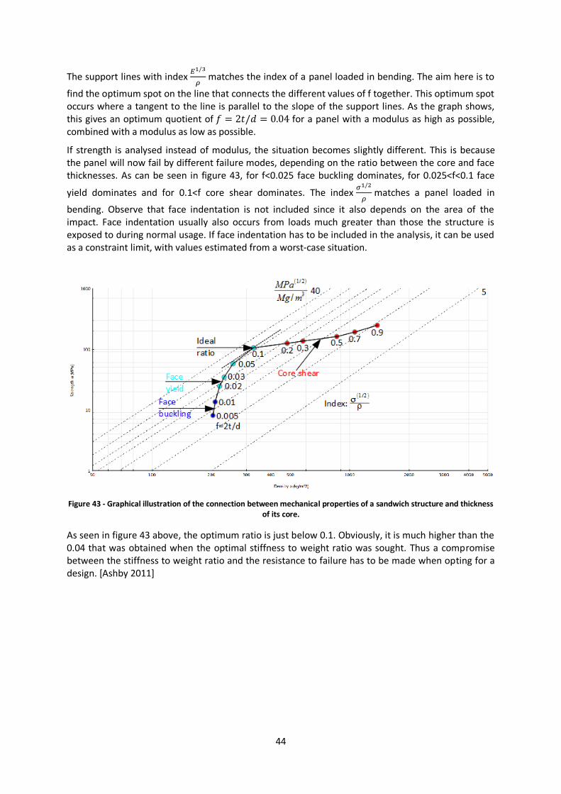
44
The support lines with index 𝐸1/3
𝜌 matches the index of a panel loaded in bending. The aim here is to
find the optimum spot on the line that connects the different values of f together. This optimum spot occurs where a tangent to the line is parallel to the slope of the support lines. As the graph shows, this gives an optimum quotient of 𝑓 = 2𝑡/𝑑 = 0.04 for a panel with a modulus as high as possible, combined with a modulus as low as possible.
If strength is analysed instead of modulus, the situation becomes slightly different. This is because the panel will now fail by different failure modes, depending on the ratio between the core and face thicknesses. As can be seen in figure 43, for f<0.025 face buckling dominates, for 0.025<f<0.1 face
yield dominates and for 0.1<f core shear dominates. The index 𝜎1/2
𝜌 matches a panel loaded in
bending. Observe that face indentation is not included since it also depends on the area of the impact. Face indentation usually also occurs from loads much greater than those the structure is exposed to during normal usage. If face indentation has to be included in the analysis, it can be used as a constraint limit, with values estimated from a worst-case situation.
Figure 43 - Graphical illustration of the connection between mechanical properties of a sandwich structure and thickness of its core.
As seen in figure 43 above, the optimum ratio is just below 0.1. Obviously, it is much higher than the 0.04 that was obtained when the optimal stiffness to weight ratio was sought. Thus a compromise between the stiffness to weight ratio and the resistance to failure has to be made when opting for a design. [Ashby 2011]
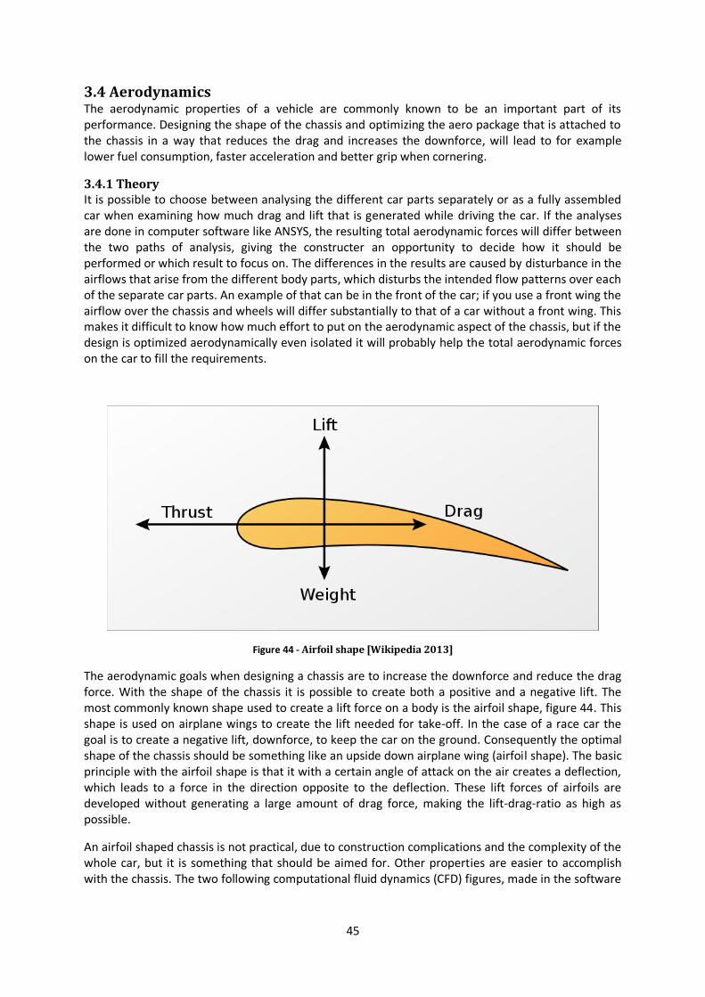
45
3.4 Aerodynamics The aerodynamic properties of a vehicle are commonly known to be an important part of its performance. Designing the shape of the chassis and optimizing the aero package that is attached to the chassis in a way that reduces the drag and increases the downforce, will lead to for example lower fuel consumption, faster acceleration and better grip when cornering.
3.4.1 Theory It is possible to choose between analysing the different car parts separately or as a fully assembled car when examining how much drag and lift that is generated while driving the car. If the analyses are done in computer software like ANSYS, the resulting total aerodynamic forces will differ between the two paths of analysis, giving the constructer an opportunity to decide how it should be performed or which result to focus on. The differences in the results are caused by disturbance in the airflows that arise from the different body parts, which disturbs the intended flow patterns over each of the separate car parts. An example of that can be in the front of the car; if you use a front wing the airflow over the chassis and wheels will differ substantially to that of a car without a front wing. This makes it difficult to know how much effort to put on the aerodynamic aspect of the chassis, but if the design is optimized aerodynamically even isolated it will probably help the total aerodynamic forces on the car to fill the requirements.
Figure 44 - Airfoil shape [Wikipedia 2013]
The aerodynamic goals when designing a chassis are to increase the downforce and reduce the drag force. With the shape of the chassis it is possible to create both a positive and a negative lift. The most commonly known shape used to create a lift force on a body is the airfoil shape, figure 44. This shape is used on airplane wings to create the lift needed for take-off. In the case of a race car the goal is to create a negative lift, downforce, to keep the car on the ground. Consequently the optimal shape of the chassis should be something like an upside down airplane wing (airfoil shape). The basic principle with the airfoil shape is that it with a certain angle of attack on the air creates a deflection, which leads to a force in the direction opposite to the deflection. These lift forces of airfoils are developed without generating a large amount of drag force, making the lift-drag-ratio as high as possible.
An airfoil shaped chassis is not practical, due to construction complications and the complexity of the whole car, but it is something that should be aimed for. Other properties are easier to accomplish with the chassis. The two following computational fluid dynamics (CFD) figures, made in the software
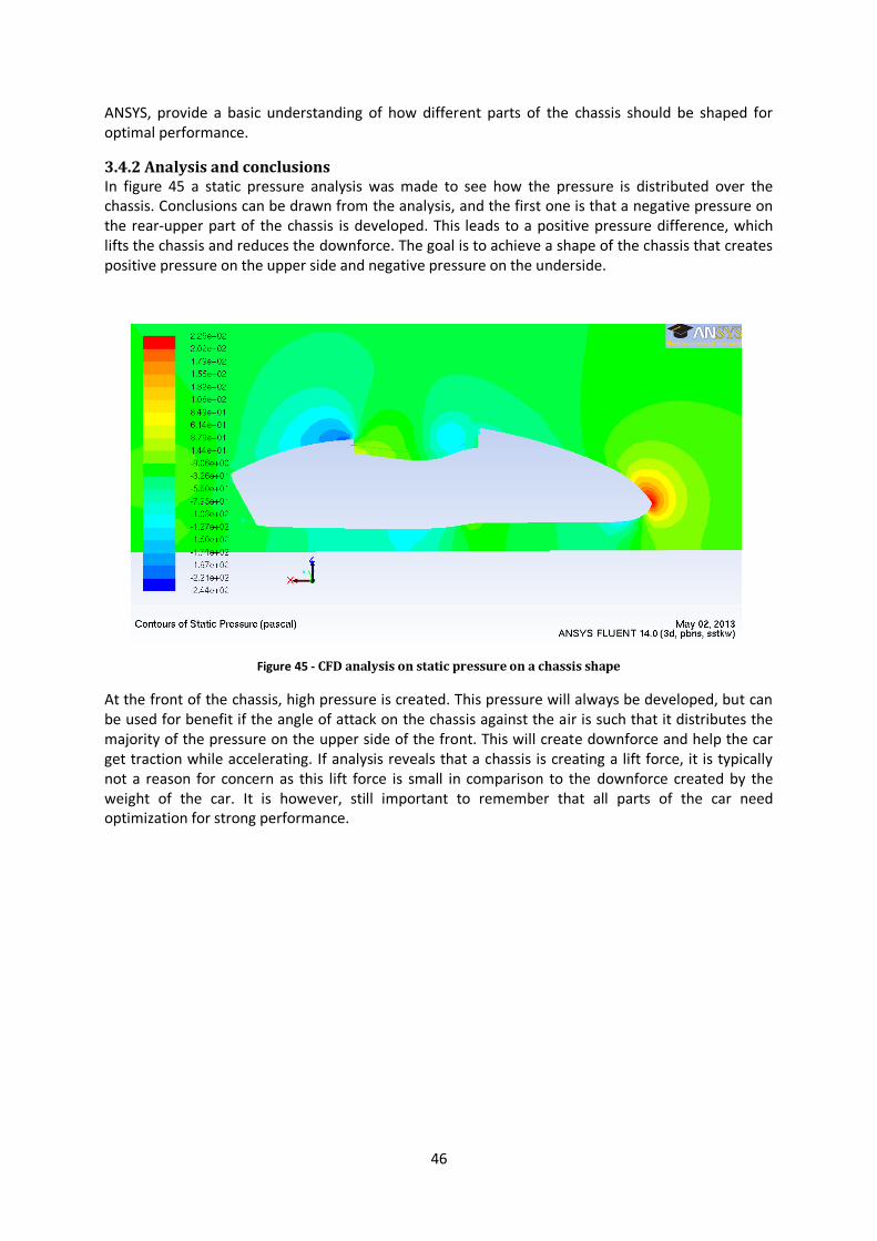
46
ANSYS, provide a basic understanding of how different parts of the chassis should be shaped for optimal performance.
3.4.2 Analysis and conclusions In figure 45 a static pressure analysis was made to see how the pressure is distributed over the chassis. Conclusions can be drawn from the analysis, and the first one is that a negative pressure on the rear-upper part of the chassis is developed. This leads to a positive pressure difference, which lifts the chassis and reduces the downforce. The goal is to achieve a shape of the chassis that creates positive pressure on the upper side and negative pressure on the underside.
Figure 45 - CFD analysis on static pressure on a chassis shape
At the front of the chassis, high pressure is created. This pressure will always be developed, but can be used for benefit if the angle of attack on the chassis against the air is such that it distributes the majority of the pressure on the upper side of the front. This will create downforce and help the car get traction while accelerating. If analysis reveals that a chassis is creating a lift force, it is typically not a reason for concern as this lift force is small in comparison to the downforce created by the weight of the car. It is however, still important to remember that all parts of the car need optimization for strong performance.
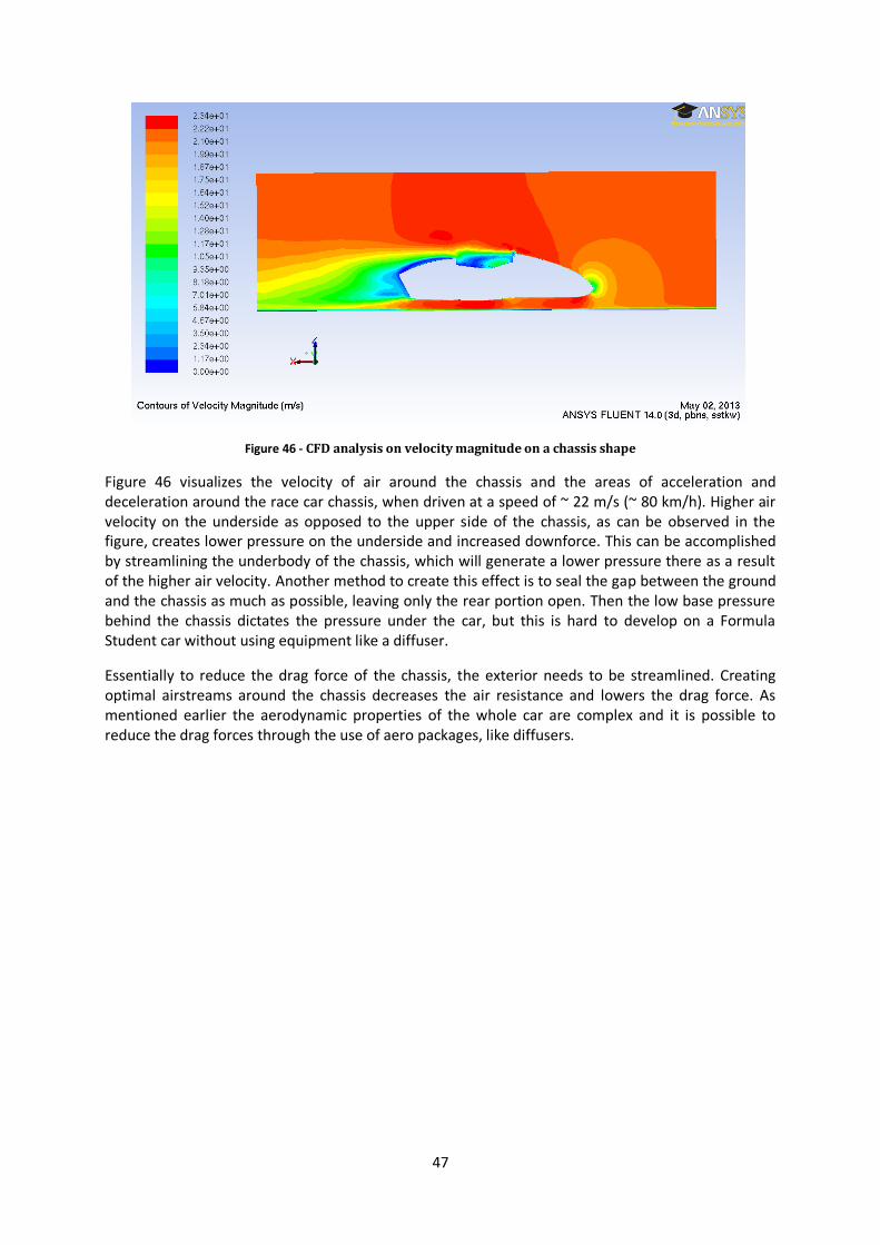
47
Figure 46 - CFD analysis on velocity magnitude on a chassis shape
Figure 46 visualizes the velocity of air around the chassis and the areas of acceleration and deceleration around the race car chassis, when driven at a speed of ~ 22 m/s (~ 80 km/h). Higher air velocity on the underside as opposed to the upper side of the chassis, as can be observed in the figure, creates lower pressure on the underside and increased downforce. This can be accomplished by streamlining the underbody of the chassis, which will generate a lower pressure there as a result of the higher air velocity. Another method to create this effect is to seal the gap between the ground and the chassis as much as possible, leaving only the rear portion open. Then the low base pressure behind the chassis dictates the pressure under the car, but this is hard to develop on a Formula Student car without using equipment like a diffuser.
Essentially to reduce the drag force of the chassis, the exterior needs to be streamlined. Creating optimal airstreams around the chassis decreases the air resistance and lowers the drag force. As mentioned earlier the aerodynamic properties of the whole car are complex and it is possible to reduce the drag forces through the use of aero packages, like diffusers.
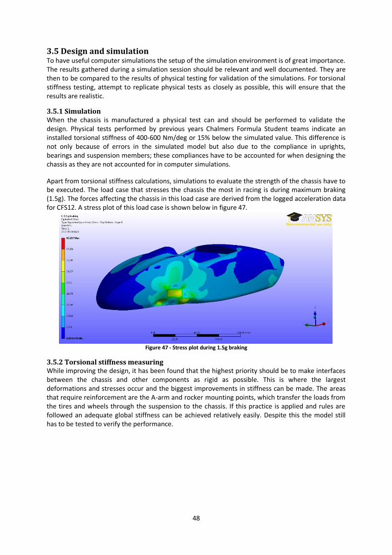
48
3.5 Design and simulation To have useful computer simulations the setup of the simulation environment is of great importance. The results gathered during a simulation session should be relevant and well documented. They are then to be compared to the results of physical testing for validation of the simulations. For torsional stiffness testing, attempt to replicate physical tests as closely as possible, this will ensure that the results are realistic.
3.5.1 Simulation When the chassis is manufactured a physical test can and should be performed to validate the design. Physical tests performed by previous years Chalmers Formula Student teams indicate an installed torsional stiffness of 400-600 Nm/deg or 15% below the simulated value. This difference is not only because of errors in the simulated model but also due to the compliance in uprights, bearings and suspension members; these compliances have to be accounted for when designing the chassis as they are not accounted for in computer simulations.
Apart from torsional stiffness calculations, simulations to evaluate the strength of the chassis have to be executed. The load case that stresses the chassis the most in racing is during maximum braking (1.5g). The forces affecting the chassis in this load case are derived from the logged acceleration data for CFS12. A stress plot of this load case is shown below in figure 47.
Figure 47 - Stress plot during 1.5g braking
3.5.2 Torsional stiffness measuring While improving the design, it has been found that the highest priority should be to make interfaces between the chassis and other components as rigid as possible. This is where the largest deformations and stresses occur and the biggest improvements in stiffness can be made. The areas that require reinforcement are the A-arm and rocker mounting points, which transfer the loads from the tires and wheels through the suspension to the chassis. If this practice is applied and rules are followed an adequate global stiffness can be achieved relatively easily. Despite this the model still has to be tested to verify the performance.
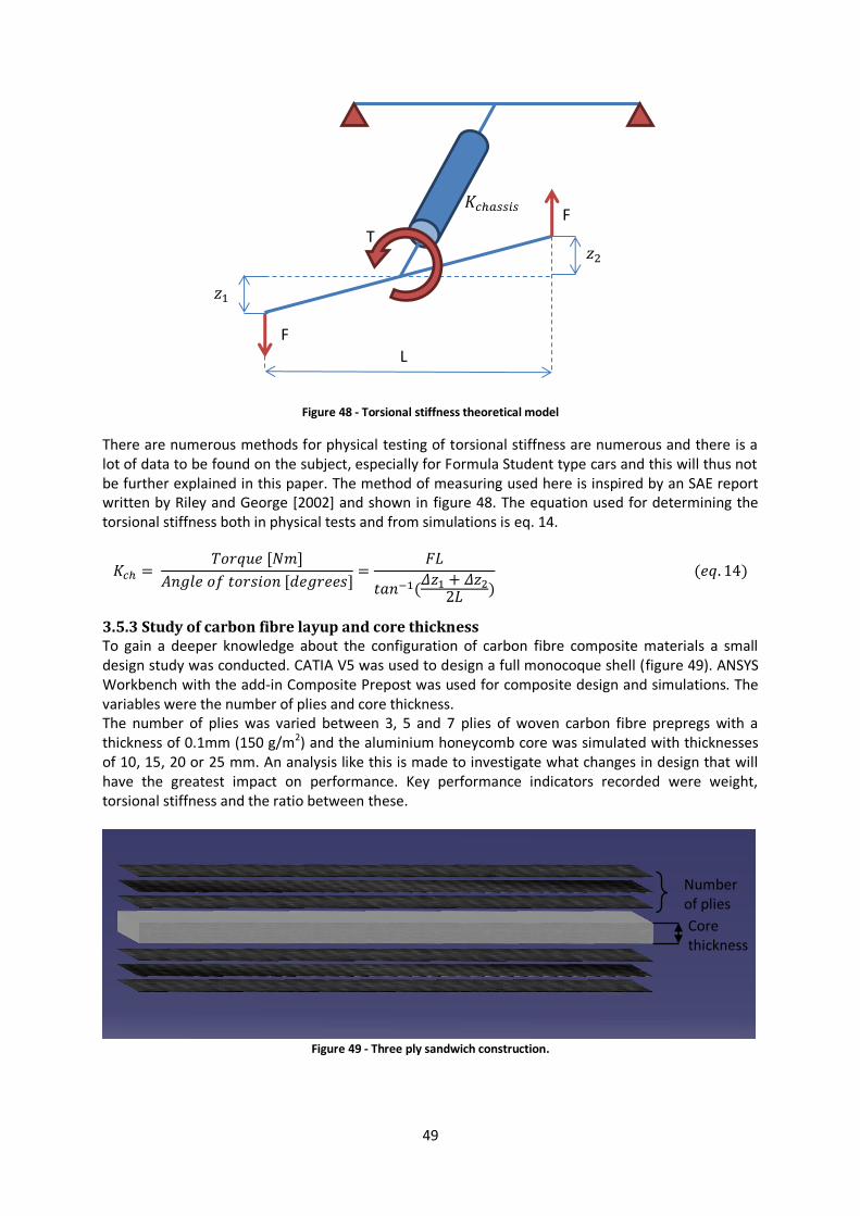
49
Figure 48 - Torsional stiffness theoretical model
There are numerous methods for physical testing of torsional stiffness are numerous and there is a lot of data to be found on the subject, especially for Formula Student type cars and this will thus not be further explained in this paper. The method of measuring used here is inspired by an SAE report written by Riley and George [2002] and shown in figure 48. The equation used for determining the torsional stiffness both in physical tests and from simulations is eq. 14.
𝐾𝑐ℎ = 𝑇𝑜𝑟𝑞𝑢𝑒 [𝑁𝑚]
𝐴𝑛𝑔𝑙𝑒 𝑜𝑓 𝑡𝑜𝑟𝑠𝑖𝑜𝑛 [𝑑𝑒𝑔𝑟𝑒𝑒𝑠]=
𝐹𝐿
𝑡𝑎𝑛−1(𝛥𝑧1 + 𝛥𝑧2
2𝐿 ) (𝑒𝑞. 14)
3.5.3 Study of carbon fibre layup and core thickness To gain a deeper knowledge about the configuration of carbon fibre composite materials a small design study was conducted. CATIA V5 was used to design a full monocoque shell (figure 49). ANSYS Workbench with the add-in Composite Prepost was used for composite design and simulations. The variables were the number of plies and core thickness. The number of plies was varied between 3, 5 and 7 plies of woven carbon fibre prepregs with a thickness of 0.1mm (150 g/m2) and the aluminium honeycomb core was simulated with thicknesses of 10, 15, 20 or 25 mm. An analysis like this is made to investigate what changes in design that will have the greatest impact on performance. Key performance indicators recorded were weight, torsional stiffness and the ratio between these.
Figure 49 - Three ply sandwich construction.
F
F
𝑧1
𝑧2
L
T
𝐾𝑐ℎ𝑎𝑠𝑠𝑖𝑠
Number of plies
Core thickness
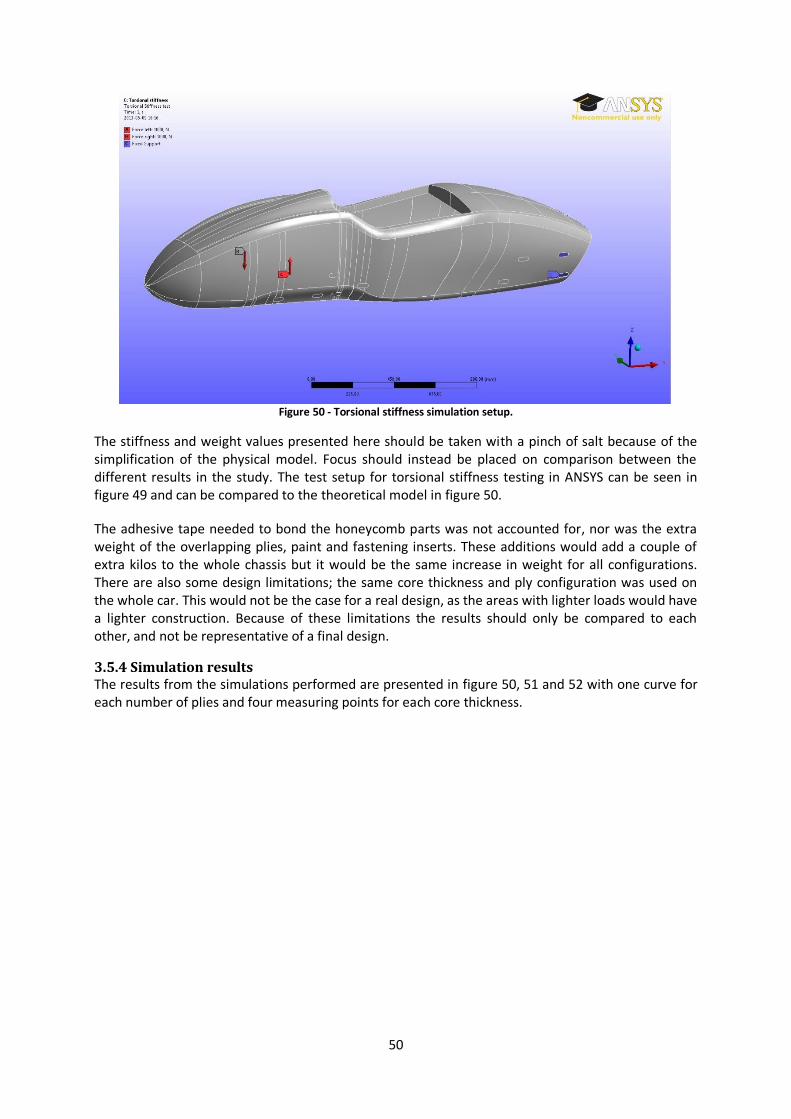
50
Figure 50 - Torsional stiffness simulation setup.
The stiffness and weight values presented here should be taken with a pinch of salt because of the simplification of the physical model. Focus should instead be placed on comparison between the different results in the study. The test setup for torsional stiffness testing in ANSYS can be seen in figure 49 and can be compared to the theoretical model in figure 50.
The adhesive tape needed to bond the honeycomb parts was not accounted for, nor was the extra weight of the overlapping plies, paint and fastening inserts. These additions would add a couple of extra kilos to the whole chassis but it would be the same increase in weight for all configurations. There are also some design limitations; the same core thickness and ply configuration was used on the whole car. This would not be the case for a real design, as the areas with lighter loads would have a lighter construction. Because of these limitations the results should only be compared to each other, and not be representative of a final design.
3.5.4 Simulation results The results from the simulations performed are presented in figure 50, 51 and 52 with one curve for each number of plies and four measuring points for each core thickness.
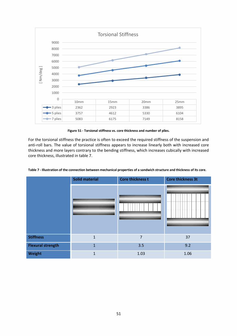
51
Figure 51 - Torsional stiffness vs. core thickness and number of plies.
For the torsional stiffness the practice is often to exceed the required stiffness of the suspension and anti-roll bars. The value of torsional stiffness appears to increase linearly both with increased core thickness and more layers contrary to the bending stiffness, which increases cubically with increased core thickness, illustrated in table 7.
Table 7 - Illustration of the connection between mechanical properties of a sandwich structure and thickness of its core.
Solid material Core thickness t Core thickness 3t
Stiffness 1 7 37
Flexural strength 1 3.5 9.2
Weight 1 1.03 1.06
10mm 15mm 20mm 25mm
3 plies 2362 2923 3386 3895
5 plies 3757 4612 5330 6104
7 plies 5083 6175 7149 8158
0
1000
2000
3000
4000
5000
6000
7000
8000
9000[
Nm
/deg
]
Torsional Stiffness
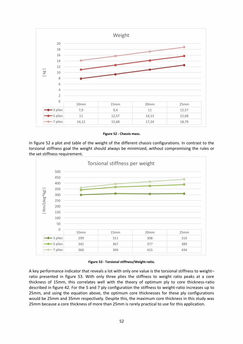
52
Figure 52 - Chassis mass.
In figure 52 a plot and table of the weight of the different chassis configurations. In contrast to the torsional stiffness goal the weight should always be minimized, without compromising the rules or the set stiffness requirement.
Figure 53 - Torsional stiffness/Weight-ratio.
A key performance indicator that reveals a lot with only one value is the torsional stiffness to weight–ratio presented in figure 53. With only three plies the stiffness to weight ratio peaks at a core thickness of 15mm, this correlates well with the theory of optimum ply to core thickness-ratio described in figure 42. For the 5 and 7 ply configuration the stiffness to weight-ratio increases up to 25mm, and using the equation above, the optimum core thicknesses for these ply configurations would be 25mm and 35mm respectively. Despite this, the maximum core thickness in this study was 25mm because a core thickness of more than 25mm is rarely practical to use for this application.
10mm 15mm 20mm 25mm
3 plies 7,9 9,4 11 12,57
5 plies 11 12,57 14,13 15,68
7 plies 14,12 15,68 17,24 18,79
0
2
4
6
8
10
12
14
16
18
20[
kg ]
Weight
10mm 15mm 20mm 25mm
3 plies 299 311 308 310
5 plies 342 367 377 389
7 plies 360 394 415 434
0
50
100
150
200
250
300
350
400
450
500
[ N
m/(
deg
*kg)
]
Torsional stiffness per weight
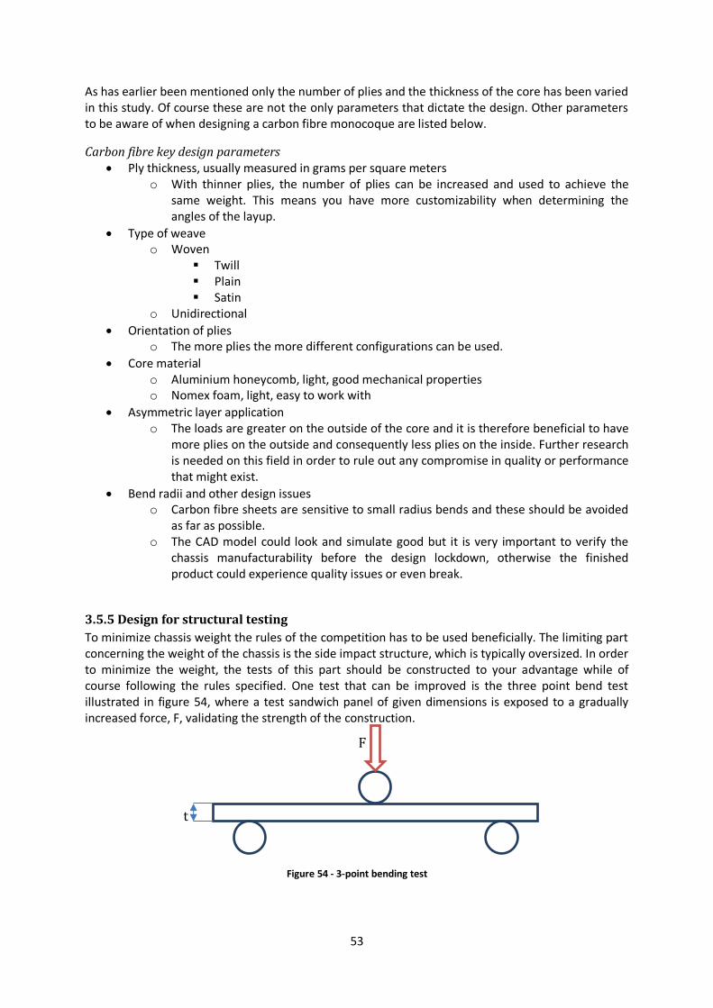
53
As has earlier been mentioned only the number of plies and the thickness of the core has been varied in this study. Of course these are not the only parameters that dictate the design. Other parameters to be aware of when designing a carbon fibre monocoque are listed below.
Carbon fibre key design parameters Ply thickness, usually measured in grams per square meters
o With thinner plies, the number of plies can be increased and used to achieve the same weight. This means you have more customizability when determining the angles of the layup.
Type of weave o Woven
Twill Plain Satin
o Unidirectional
Orientation of plies o The more plies the more different configurations can be used.
Core material o Aluminium honeycomb, light, good mechanical properties o Nomex foam, light, easy to work with
Asymmetric layer application o The loads are greater on the outside of the core and it is therefore beneficial to have
more plies on the outside and consequently less plies on the inside. Further research is needed on this field in order to rule out any compromise in quality or performance that might exist.
Bend radii and other design issues o Carbon fibre sheets are sensitive to small radius bends and these should be avoided
as far as possible. o The CAD model could look and simulate good but it is very important to verify the
chassis manufacturability before the design lockdown, otherwise the finished product could experience quality issues or even break.
3.5.5 Design for structural testing
To minimize chassis weight the rules of the competition has to be used beneficially. The limiting part concerning the weight of the chassis is the side impact structure, which is typically oversized. In order to minimize the weight, the tests of this part should be constructed to your advantage while of course following the rules specified. One test that can be improved is the three point bend test illustrated in figure 54, where a test sandwich panel of given dimensions is exposed to a gradually increased force, F, validating the strength of the construction.
Figure 54 - 3-point bending test
t
F
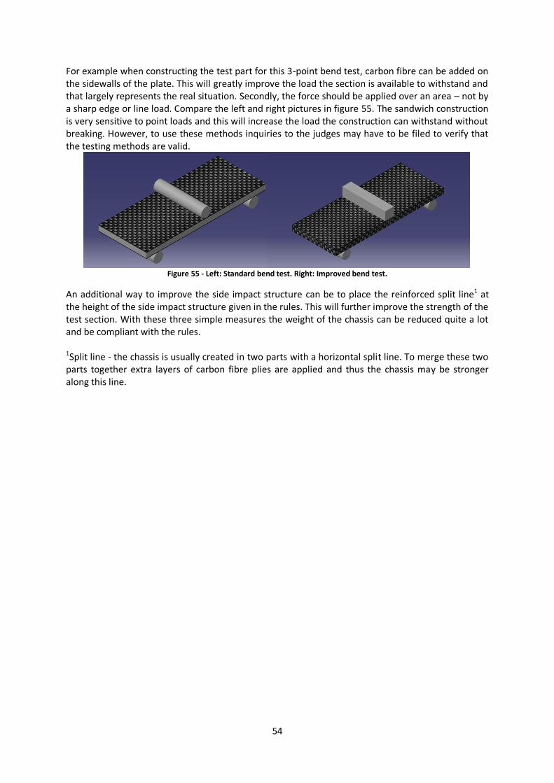
54
For example when constructing the test part for this 3-point bend test, carbon fibre can be added on the sidewalls of the plate. This will greatly improve the load the section is available to withstand and that largely represents the real situation. Secondly, the force should be applied over an area – not by a sharp edge or line load. Compare the left and right pictures in figure 55. The sandwich construction is very sensitive to point loads and this will increase the load the construction can withstand without breaking. However, to use these methods inquiries to the judges may have to be filed to verify that the testing methods are valid.
Figure 55 - Left: Standard bend test. Right: Improved bend test.
An additional way to improve the side impact structure can be to place the reinforced split line1 at the height of the side impact structure given in the rules. This will further improve the strength of the test section. With these three simple measures the weight of the chassis can be reduced quite a lot and be compliant with the rules.
1Split line - the chassis is usually created in two parts with a horizontal split line. To merge these two parts together extra layers of carbon fibre plies are applied and thus the chassis may be stronger along this line.
55
3.6 Carbon Composite Monocoque Chassis Design Being the central element of the car, the monocoque is perhaps the key to a race car’s overall performance. As explained by the functional model, other load bearing components are attached to the monocoque, and the chassis have to absorb and react to a multitude of forces.
A carbon composite monocoque chassis offers several advantages over the more traditional space frame, but to effectively capitalize on these strengths, it is important to adopt a well thought through, structured design approach.
3.6.1 Advantages As the chassis is an integral backbone of the race car, it presents an excellent opportunity for weight savings - a must for efficient and powerful performance. By opting for a composite monocoque chassis substantial amounts of weight can be saved. This weight saving is perhaps best exemplified by the fact that carbon fibre composites amount for almost 85% of the volume of a contemporary formula 1 car whilst accounting for less than 25% of its mass. [Savage 2008] In addition to the reduction of weight, a composite monocoque also provides the inherent opportunity of a lower centre of gravity. As a racing car is constantly accelerating, be it positively or negatively, the lower centre of gravity directly affects its handling characteristics. Carbon fibre composites are fibrous, offering high strength and stiffness, with the fibres acting as the principal load-bearing constituent. A composite structure is designed to have a precisely defined quantity of fibres in the correct location and orientation, with a minimum of polymer to provide support. Thus a carbon composite monocoque offers significant rigidity and stiffness whilst also having a low weight. As the monocoque is both the chassis, and the body of the race car, it greatly reduces the complexity of design and packaging. Composed of essentially one part (depending on the chosen approach to manufacturing), a monocoque allows for a more modular assembly strategy, saving time and resources. Carbon composite monocoque manufacture is however still a relatively new area and if attempted without sufficient expertise, production may be tedious and time consuming with questionable quality. In summary, a well-designed carbon composite monocoque is light, stiff, rigid and when mastered, simple. To tap in on these advantages it is imperative to have a rigorous, well-defined design phase.
3.6.2 Design Process The design phase for a composite monocoque chassis should ideally be rigorous and all-encompassing to ensure optimal performance and ease-of-manufacturability. Figure 57 below provides a visual outline for the design phase.
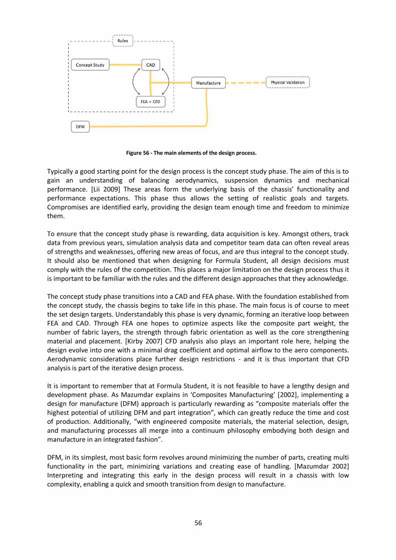
56
Typically a good starting point for the design process is the concept study phase. The aim of this is to gain an understanding of balancing aerodynamics, suspension dynamics and mechanical performance. [Lii 2009] These areas form the underlying basis of the chassis’ functionality and performance expectations. This phase thus allows the setting of realistic goals and targets. Compromises are identified early, providing the design team enough time and freedom to minimize them. To ensure that the concept study phase is rewarding, data acquisition is key. Amongst others, track data from previous years, simulation analysis data and competitor team data can often reveal areas of strengths and weaknesses, offering new areas of focus, and are thus integral to the concept study. It should also be mentioned that when designing for Formula Student, all design decisions must comply with the rules of the competition. This places a major limitation on the design process thus it is important to be familiar with the rules and the different design approaches that they acknowledge. The concept study phase transitions into a CAD and FEA phase. With the foundation established from the concept study, the chassis begins to take life in this phase. The main focus is of course to meet the set design targets. Understandably this phase is very dynamic, forming an iterative loop between FEA and CAD. Through FEA one hopes to optimize aspects like the composite part weight, the number of fabric layers, the strength through fabric orientation as well as the core strengthening material and placement. [Kirby 2007] CFD analysis also plays an important role here, helping the design evolve into one with a minimal drag coefficient and optimal airflow to the aero components. Aerodynamic considerations place further design restrictions - and it is thus important that CFD analysis is part of the iterative design process. It is important to remember that at Formula Student, it is not feasible to have a lengthy design and development phase. As Mazumdar explains in ‘Composites Manufacturing’ [2002], implementing a design for manufacture (DFM) approach is particularly rewarding as “composite materials offer the highest potential of utilizing DFM and part integration”, which can greatly reduce the time and cost of production. Additionally, “with engineered composite materials, the material selection, design, and manufacturing processes all merge into a continuum philosophy embodying both design and manufacture in an integrated fashion”. DFM, in its simplest, most basic form revolves around minimizing the number of parts, creating multi functionality in the part, minimizing variations and creating ease of handling. [Mazumdar 2002] Interpreting and integrating this early in the design process will result in a chassis with low complexity, enabling a quick and smooth transition from design to manufacture.
Figure 56 - The main elements of the design process.
57
Physical testing is an important part of design validation but due to the nature of the Formula Student project, allocating resources for the manufacture and testing of components is difficult. It is thus important that the design phase accounts for real-world factors that can potentially hamper performance.
3.6.3 Design Attributes
This section aims to present various carbon composite monocoque chassis design attributes and details that are sometimes overlooked. All of these attributes need not be necessarily implemented, but should instead be treated as pointers for good chassis design.
• The carbon composites should be handled with care as the strength of the material is maximized when imperfections are kept to a minimum. Surface damage (like cracks) is detrimental to the strength - especially when perpendicular to the applied loads.
• Long continuous fibres are preferred. They are the principal load-bearing constituent in the direction of the load and thus are integral to the chassis performance. Fibre discontinuities result in reduced mechanical performance.
• Woven composite structures offer: ease of conformance to complex geometries, reduced manufacturing time and improved damage resistance. Woven ply offers superior topology optimization, with its much wider spread. [Savage 2008]
• Allowing the inner and outer skins of the monocoque to be in a ± 45° arrangement typically offers superior chassis torsional stiffness.
• The core occupies most of the volume. Two of the most important mechanical core properties: out of plane compressional strength and its shear moduli. [Grimes 2011]
• As part of the DFM strategy, the geometry of the chassis must maintain easy drapability. Some geometry may not allow for plies to form around them. By ensuring that the draft angle is sufficiently generous (1° is recommended for vertical surfaces) warpage is reduced. It also facilitates easier removal of the monocoque from the mould. [Mazumdar 2002]
• Corners are critical regions. Lii [2009] explains that the strength of the carbon composite is dominated by the tensile strength of the fibres and around corners this strength is impacted negatively. Honeycomb cores also face a complex situation at corners as they typically bend better in certain directions. Corners with large radii offer better manufacturability. Mazumdar [2002] indicates that a minimum inside corner radii of ~2 mm and minimum outside corner radii of ~1.5 mm are recommended.
• Monocoque chassis resolve loads poorly when fed perpendicularly into the skin and this should be avoided. The design must allow loads to be absorbed into the direction of the fibres.
It should also be noted that whilst a successful design phase will see the initial performance and stiffness goals be met, the installed stiffness of the chassis will be considerably less. [Clarke 2010] The installed stiffness is measured at the hubs - introducing compliances and clearance stacking from the suspension and linkage components attached to the monocoque. By keeping this in mind and tackling these issues right from the onset of the design phase, immediate gains in handling and drivability can be had.
3.7 Manufacturing Design in all its glory, but no product can ever work properly if the designed part cannot be manufactured. CFS13 suffered from manufacturing mistakes and timetable setbacks due to the lack of manufacturing experience. Therefore, this section will focus on manufacturing concerns and design shapes with the purpose of simplifying the process.
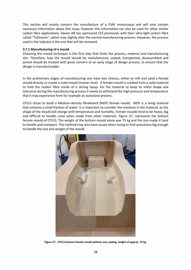
58
This section will mostly concern the manufacture of a FSAE monocoque and will only contain necessary information about this issue; however this information can also be used for other similar carbon fibre applications. Oxeon AB has sponsored CFS previously with their ultra-light carbon fibre called “TeXtreme”, which may slightly alter the normal manufacturing process. However, the process used in the industry is the one that will be reviewed.
3.7.1 Manufacturing of a mould Choosing the mould technique is the first step that limits the process, material and manufacturing site. Therefore, how the mould should be manufactured, coated, transported, disassembled and joined should be treated with great concern at an early stage of design process, to ensure that the design is manufacturable.
In the preliminary stages of manufacturing one have two choices, either to mill and sand a female mould directly or create a male mould (master-tool). A female mould is created from a solid material to hold the carbon fibre inside of it during layup. For the material to keep its initial shape and tolerance during the manufacturing process it needs to withstand the high pressure and temperature that it may experience from for example an autoclave process.
CFS13 chose to build a Medium-density fibreboard (MDF) female mould. MDF is a living material that contains a small fraction of water. It is important to consider the moisture in the material, as the shape of the mould will change with temperature and humidity. Female moulds tend to be heavy, big and difficult to handle, even when made from other materials. Figure 57, represents the bottom female mould of CFS13. The weight of the bottom mould alone was 75 kg and the size made it hard to handle and transport. This method may also have issues when trying to find autoclaves big enough to handle the size and weight of the mould.
Figure 57 - CFS13 bottom female mould without any coating, weight of approx. 75 kg.
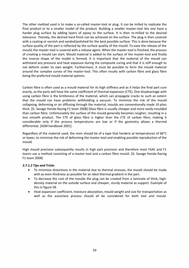
59
The other method used is to make a so-called master-tool or plug. It can be milled to replicate the final product or to a smaller model of the product. Building a smaller master-tool lets one have a harder plug surface by adding layers of epoxy to the surface. It is then re-milled to the desired tolerance. Thereby, the desired hard finish can be achieved on the surface. The plug is then covered with a coating or varnish and sanded/polished for the best possible surface. This is done because the surface quality of the part is reflected by the surface quality of the mould. To ease the release of the mould, the master-tool is covered with a release agent. When the master-tool is finished, the process of creating a mould can start. Mould material is added to the surface of the master-tool and finally the inverse shape of the model is formed. It is important that the material of the mould can withstand any pressure and heat exposure during the composite curing and that it is stiff enough to not deform under its own weight. Furthermore, it must be possible to form the mould material around the complex curves of the master-tool. This often results with carbon fibre and glass fibre being the preferred mould material options.
Carbon fibre is often used as a mould material for its high stiffness and as it helps the final part cure evenly, as the parts will have the same coefficient of thermal expansion (CTE). One disadvantage with using carbon fibre is the brittleness of the material, which can propagate cracks to such an extent that the mould can have problems withholding a vacuum. To minimize the risk of the mould collapsing, deforming or air diffusing through the material, moulds are conventionally made 10 plies thick. [G. Savage Honda Racing F1 team 2008] Glass fibre is usually cheaper and more easily moulded than carbon fibre. Unfortunately the surface of the mould generally becomes rougher, resulting in a less smooth product. The CTE of glass fibre is higher than the CTE of carbon fibre, making it considerable only if the process temperatures are low or if the geometry allows a thermal differential. [ASM handbook 2001]
Regardless of the material used, the resin should be of a type that hardens at temperatures of 60°C or lower, to minimize the risk of deforming the master-tool and enabling possible reproduction of the mould.
High mould precision subsequently results in high part precision and therefore most FSAE and F1 teams use a method consisting of a master-tool and a carbon fibre mould. [G. Savage Honda Racing F1 team 2008]
3.7.1.2 Tips and Tricks
To minimize distortions in the material due to thermal stresses, the mould should be made with as even thickness as possible for an ideal thermal gradient in the part.
To decrease the cost of the moulds the plug can be created from a laminate of thick, high-density material on the outside surface and cheaper, sturdy material as support. Example of this in figure 58.
Heat expansion coefficient, moisture absorption, mould weight and size for transportation as well as the autoclave process should all be considered for both tool and mould.
60
Figure 58 - Lamination of different mould materials.
3.7.2 Manufacturing of the monocoque
3.7.2.1 Basic steps for carbon fibre manufacturing
Impregnation The first step is to mix the matrix (resin) and the fibres into a laminate. This could either be done by brushing mixed matrix onto a dry carbon fibre sheet, or be pre-impregnated by the supplier (prepreg).
Layup In this second step, the composite laminate is formed after the designed shape. It is often done in a mould; by placing carbon fibre plies in the desired angle on top of each other. The direction of the fibres, placement of the plies and the number of layers should be added according to the manufacturing plan, called the plybook. Such plans can be automatically generated from composite analysis software, for example ANSYS Composite Prepost (ACP).
Consolidation The third step is the consolidation, where the composite plies create intimate connections with each other. This can be achieved by using rollers, a vacuum or pressure on top of the plies, forcing them together. A better consolidated product gives better mechanical properties.
Solidification The final step is the solidification. The duration of the process can vary from a few minutes at room temperature to several hours in an autoclave, at high pressure and temperature. This step may vary depending on the matrix material. It is important to always follow recommendations of the resin manufacturer. Failing to follow the recommendations may cause stresses and/or failed mechanical properties in the finished part. [ASM handbook 2001]
3.7.2.2 Advanced processes
Prepreg Prepreg is short for carbon fibre pre-impregnated with resin. It is an advanced process mostly used in the aerospace industry and by prototype manufacturers.
The prepreg method is expensive and labour intensive, but gives a great stiffness-to-weight ratio due to its high fibre volume fraction (~60-65%). [Mazumdar 2002] Unfortunately it requires a few very
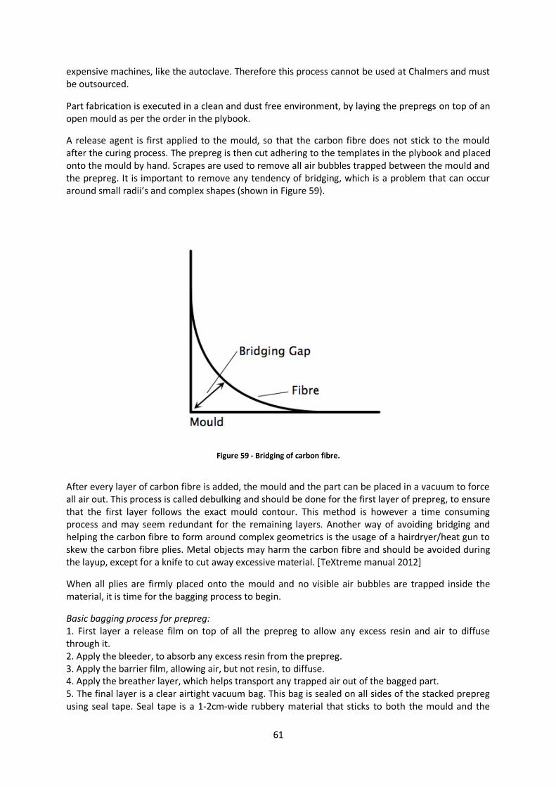
61
expensive machines, like the autoclave. Therefore this process cannot be used at Chalmers and must be outsourced.
Part fabrication is executed in a clean and dust free environment, by laying the prepregs on top of an open mould as per the order in the plybook.
A release agent is first applied to the mould, so that the carbon fibre does not stick to the mould after the curing process. The prepreg is then cut adhering to the templates in the plybook and placed onto the mould by hand. Scrapes are used to remove all air bubbles trapped between the mould and the prepreg. It is important to remove any tendency of bridging, which is a problem that can occur around small radii’s and complex shapes (shown in Figure 59).
Figure 59 - Bridging of carbon fibre.
After every layer of carbon fibre is added, the mould and the part can be placed in a vacuum to force all air out. This process is called debulking and should be done for the first layer of prepreg, to ensure that the first layer follows the exact mould contour. This method is however a time consuming process and may seem redundant for the remaining layers. Another way of avoiding bridging and helping the carbon fibre to form around complex geometrics is the usage of a hairdryer/heat gun to skew the carbon fibre plies. Metal objects may harm the carbon fibre and should be avoided during the layup, except for a knife to cut away excessive material. [TeXtreme manual 2012]
When all plies are firmly placed onto the mould and no visible air bubbles are trapped inside the material, it is time for the bagging process to begin.
Basic bagging process for prepreg: 1. First layer a release film on top of all the prepreg to allow any excess resin and air to diffuse through it. 2. Apply the bleeder, to absorb any excess resin from the prepreg. 3. Apply the barrier film, allowing air, but not resin, to diffuse. 4. Apply the breather layer, which helps transport any trapped air out of the bagged part. 5. The final layer is a clear airtight vacuum bag. This bag is sealed on all sides of the stacked prepreg using seal tape. Seal tape is a 1-2cm-wide rubbery material that sticks to both the mould and the
62
vacuum bag. 6. A nozzle is inserted into the vacuum bag through a small hole and sealed with seal tape. The nozzle is then connected to a vacuum hose to create vacuum inside the bag.
Basic part manufacturing using prepreg with autoclave process: 1. The prepreg is removed from the refrigerator and is kept at room temperature for thawing to avoid condensation. 2. The prepreg is laid on the cutting table and cut to the desired size and orientation. 3. The mould is cleaned and the release agent is applied to the mould surface. 4. Backing paper from the prepreg is removed and the prepreg is laid on the mould surface as per the sequence in the plybook. 5. Captured air between prepreg sheets is removed by using a squeezing roller or scrape after each prepreg sheet has been applied. 6. After applying all the prepreg sheets, the vacuum bagging arrangements are made as mentioned above. 7. The entire assembly is then placed into the autoclave. 8. Connections to thermocouples and vacuum hoses are made and the autoclave door is closed. 9. The cure cycle data is entered into the autoclave computer. 10. After cooling, the vacuum bag is removed and the part is taken out.
Tips and Tricks The coating and release material on the mould must be able to withstand any temperature
or pressure that the mould may encounter, which is that of the autoclave.
To prevent deformations, any holes should be cut after curing the part.
The kit of prepreg pieces supplied to the laminators is generally cut slightly oversized so that it can be trimmed to create precisely the correct amount of overlap.
The overlap between each sheet is normally 2-10 mm [ASM handbook 2001]
Carbon/epoxy is much lighter and stronger than other prepreg materials and provides greater mass savings in the component.
Infusion An alternative to the prepreg process is the infusion or resin infusion process. It is a cheap manufacturing process, which can be implemented at room temperatures. Furthermore, the fibre volume fraction ratio is close to that of the prepreg (50-55%) and the surface finish of the product is outstanding if the infusion process is performed correctly.
It is possible to manufacture at virtually any premises, as the method only requires a regular workshop with a vacuum pump, collector tank and bagging material. Unfortunately it is not possible at Chalmers, due to the restrictions of thermoset usage.
The initial part of the infusion process is the same as the prepreg process. The first step is to create a mould of the designed part. To ease the bagging process, a mould is manufactured with big flanges (min. 10 cm) and coated with a release agent. Dry layers of carbon fibre plies are placed into the mould and cut with a few centimetres of excess material to ensure that the material will cover the entire mould, even in a vacuum. The fibre cloth can be held fixed through the usage of tape or epoxy spray.
When all the plies are placed onto the mould it is time for the bagging process to achieve steady vacuum during the consolidation and solidification stages.
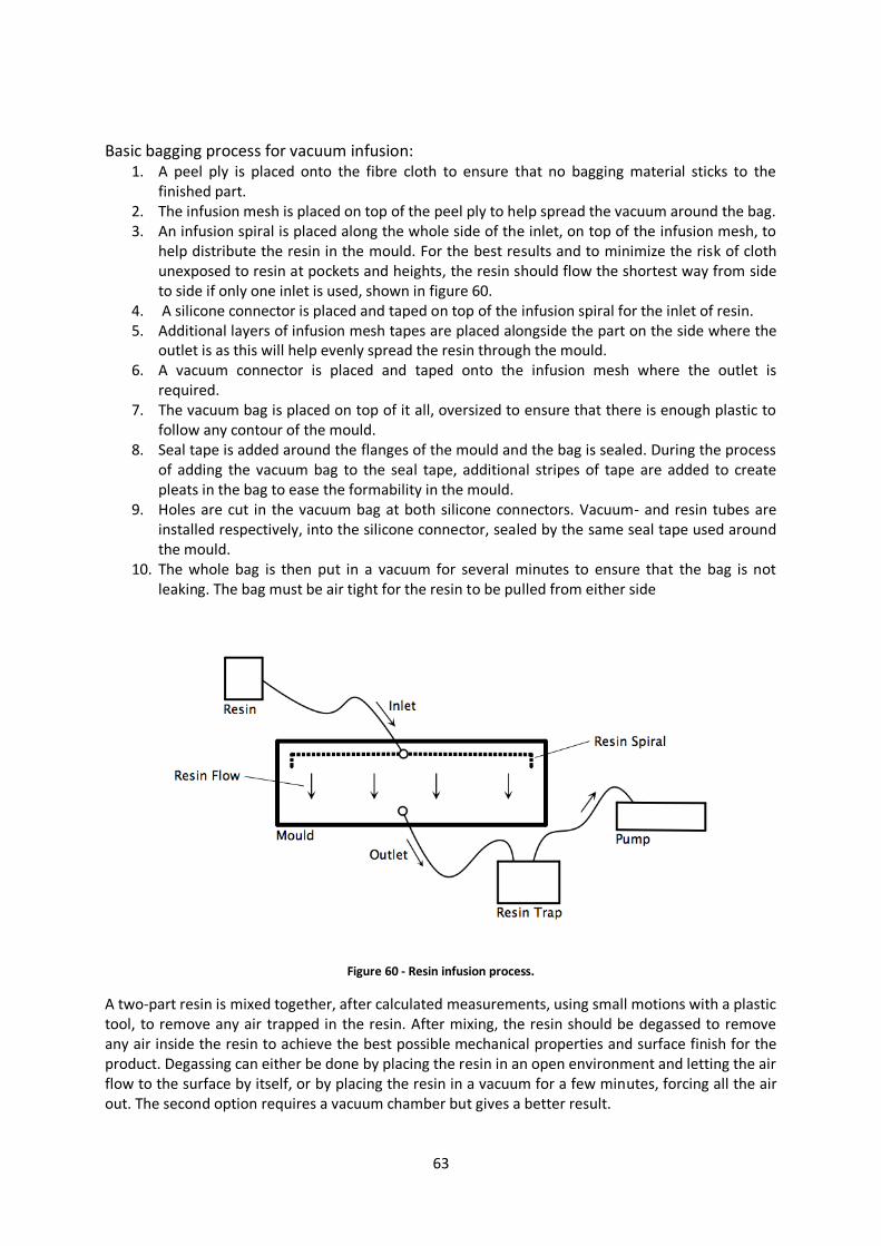
63
Basic bagging process for vacuum infusion: 1. A peel ply is placed onto the fibre cloth to ensure that no bagging material sticks to the
finished part. 2. The infusion mesh is placed on top of the peel ply to help spread the vacuum around the bag. 3. An infusion spiral is placed along the whole side of the inlet, on top of the infusion mesh, to
help distribute the resin in the mould. For the best results and to minimize the risk of cloth unexposed to resin at pockets and heights, the resin should flow the shortest way from side to side if only one inlet is used, shown in figure 60.
4. A silicone connector is placed and taped on top of the infusion spiral for the inlet of resin. 5. Additional layers of infusion mesh tapes are placed alongside the part on the side where the
outlet is as this will help evenly spread the resin through the mould. 6. A vacuum connector is placed and taped onto the infusion mesh where the outlet is
required. 7. The vacuum bag is placed on top of it all, oversized to ensure that there is enough plastic to
follow any contour of the mould. 8. Seal tape is added around the flanges of the mould and the bag is sealed. During the process
of adding the vacuum bag to the seal tape, additional stripes of tape are added to create pleats in the bag to ease the formability in the mould.
9. Holes are cut in the vacuum bag at both silicone connectors. Vacuum- and resin tubes are installed respectively, into the silicone connector, sealed by the same seal tape used around the mould.
10. The whole bag is then put in a vacuum for several minutes to ensure that the bag is not leaking. The bag must be air tight for the resin to be pulled from either side
Figure 60 - Resin infusion process.
A two-part resin is mixed together, after calculated measurements, using small motions with a plastic tool, to remove any air trapped in the resin. After mixing, the resin should be degassed to remove any air inside the resin to achieve the best possible mechanical properties and surface finish for the product. Degassing can either be done by placing the resin in an open environment and letting the air flow to the surface by itself, or by placing the resin in a vacuum for a few minutes, forcing all the air out. The second option requires a vacuum chamber but gives a better result.
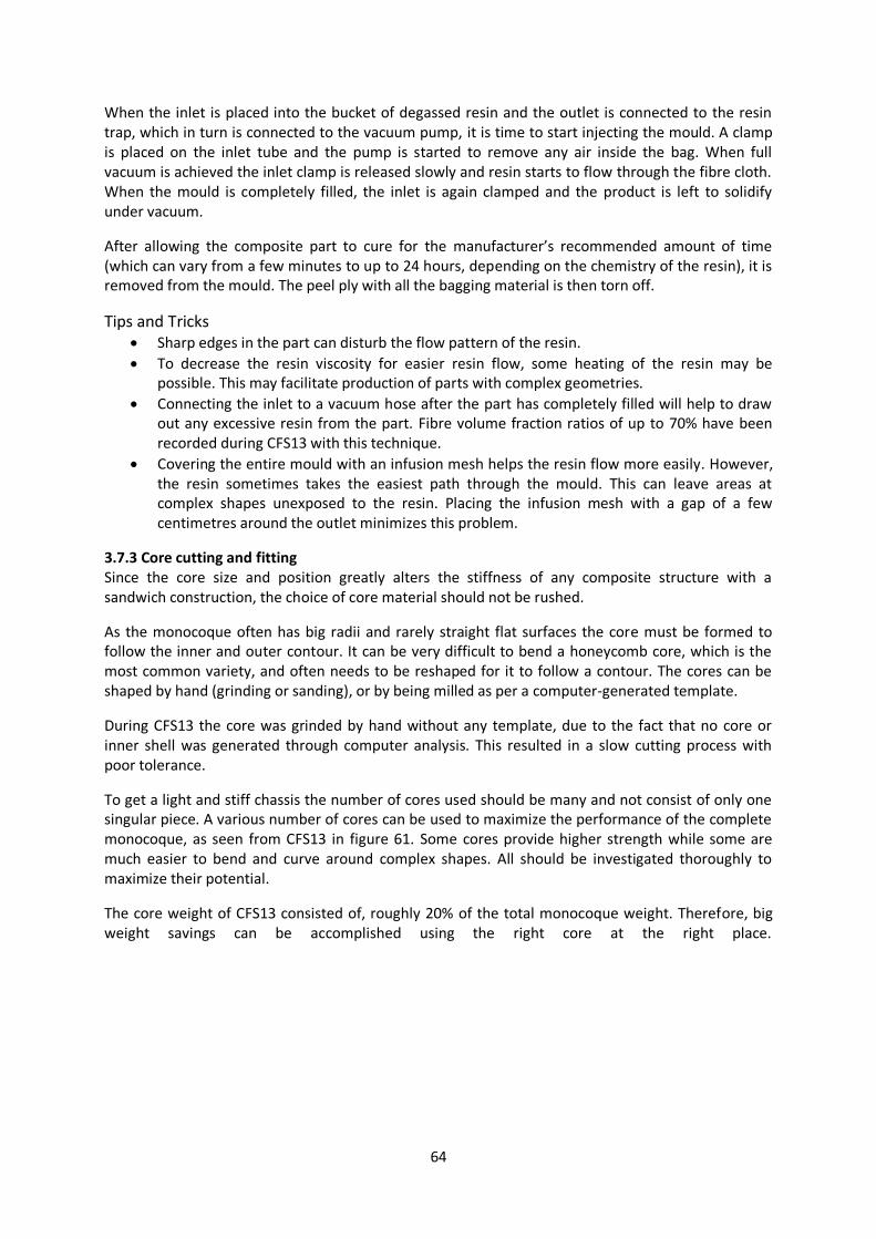
64
When the inlet is placed into the bucket of degassed resin and the outlet is connected to the resin trap, which in turn is connected to the vacuum pump, it is time to start injecting the mould. A clamp is placed on the inlet tube and the pump is started to remove any air inside the bag. When full vacuum is achieved the inlet clamp is released slowly and resin starts to flow through the fibre cloth. When the mould is completely filled, the inlet is again clamped and the product is left to solidify under vacuum.
After allowing the composite part to cure for the manufacturer’s recommended amount of time (which can vary from a few minutes to up to 24 hours, depending on the chemistry of the resin), it is removed from the mould. The peel ply with all the bagging material is then torn off.
Tips and Tricks Sharp edges in the part can disturb the flow pattern of the resin.
To decrease the resin viscosity for easier resin flow, some heating of the resin may be possible. This may facilitate production of parts with complex geometries.
Connecting the inlet to a vacuum hose after the part has completely filled will help to draw out any excessive resin from the part. Fibre volume fraction ratios of up to 70% have been recorded during CFS13 with this technique.
Covering the entire mould with an infusion mesh helps the resin flow more easily. However, the resin sometimes takes the easiest path through the mould. This can leave areas at complex shapes unexposed to the resin. Placing the infusion mesh with a gap of a few centimetres around the outlet minimizes this problem.
3.7.3 Core cutting and fitting Since the core size and position greatly alters the stiffness of any composite structure with a sandwich construction, the choice of core material should not be rushed.
As the monocoque often has big radii and rarely straight flat surfaces the core must be formed to follow the inner and outer contour. It can be very difficult to bend a honeycomb core, which is the most common variety, and often needs to be reshaped for it to follow a contour. The cores can be shaped by hand (grinding or sanding), or by being milled as per a computer-generated template.
During CFS13 the core was grinded by hand without any template, due to the fact that no core or inner shell was generated through computer analysis. This resulted in a slow cutting process with poor tolerance.
To get a light and stiff chassis the number of cores used should be many and not consist of only one singular piece. A various number of cores can be used to maximize the performance of the complete monocoque, as seen from CFS13 in figure 61. Some cores provide higher strength while some are much easier to bend and curve around complex shapes. All should be investigated thoroughly to maximize their potential.
The core weight of CFS13 consisted of, roughly 20% of the total monocoque weight. Therefore, big weight savings can be accomplished using the right core at the right place.
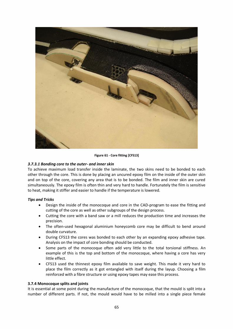
65
Figure 61 - Core fitting [CFS13]
3.7.3.1 Bonding core to the outer- and inner skin To achieve maximum load transfer inside the laminate, the two skins need to be bonded to each other through the core. This is done by placing an uncured epoxy film on the inside of the outer skin and on top of the core, covering any area that is to be bonded. The film and inner skin are cured simultaneously. The epoxy film is often thin and very hard to handle. Fortunately the film is sensitive to heat, making it stiffer and easier to handle if the temperature is lowered.
Tips and Tricks
Design the inside of the monocoque and core in the CAD-program to ease the fitting and cutting of the core as well as other subgroups of the design process.
Cutting the core with a band saw or a mill reduces the production time and increases the precision.
The often-used hexagonal aluminium honeycomb core may be difficult to bend around double curvature.
During CFS13 the cores was bonded to each other by an expanding epoxy adhesive tape. Analysis on the impact of core bonding should be conducted.
Some parts of the monocoque often add very little to the total torsional stiffness. An example of this is the top and bottom of the monocoque, where having a core has very little effect.
CFS13 used the thinnest epoxy film available to save weight. This made it very hard to place the film correctly as it got entangled with itself during the layup. Choosing a film reinforced with a fibre structure or using epoxy tapes may ease this process.
3.7.4 Monocoque splits and joints It is essential at some point during the manufacture of the monocoque, that the mould is split into a number of different parts. If not, the mould would have to be milled into a single piece female
66
mould, which is not possible with the resources of a Formula Student team and would have undesirable mechanical properties.
When choosing how the monocoque parts should be split and joined one is met with two choices:
1. Choose to make female moulds, do the layup in the moulds separately and join the parts together using a joining technique, often consisting of adhesive tape and/or glue.
2. Choose to make female moulds, joining the moulds and do one single-shell layup. This requires no joining of the parts afterwards.
Advantages using separate layups
The most obvious advantage of the separate layup is its simplicity; one has a total overview of the monocoque parts during layup and the core fitting. This also means that there can be up to 3 people working simultaneously on the mould during layup, decreasing the layup time in total.
Previous experience from CFS13.
Disadvantages
This method requires two autoclave processes for each mould, one for the outer layer and one for the inner layer. An oven is also needed for the glue and final layer to cover the joint on the inside.
As the mould is sanded the tolerance of the two final parts may discord to one another, meaning that more adhesive is needed to fill any cavities that may occur.
It often requires for the bottom or upper mould to be split into two more pieces to be able to unload the hardened part. This is due to the joint design that often requires complex curves on one side of the mould.
Often results in a line of adhesive on the outside, which may impair the surface finish of the monocoque.
Advantages using a single-shell layup
No joint is required, saving time that would otherwise be spent on design and bonding adhesives for the monocoque parts. However using this technique requires considering the joining of the mould parts.
Only requires two autoclave processes in total, making it easier to find time at sponsors, when using prepreg.
Reduction in the weight of the monocoque as no adhesive will be required for joints.
Disadvantages
Only one person can work inside the monocoque mould at a time to do the total layup and core fitting, as seen in figure 62.
It may also be quite hard to perfectly lay the plies and cores in place due to the limited working space, thus affecting the final outcome of the monocoque.
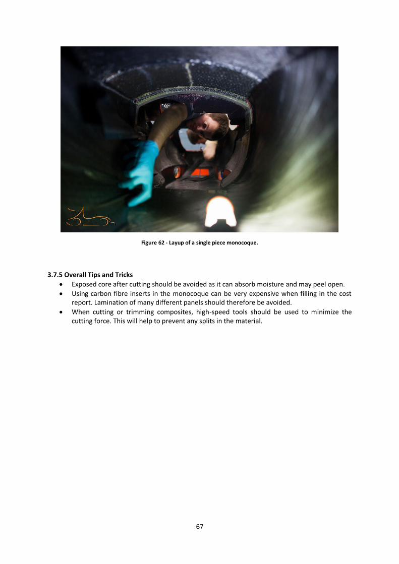
67
Figure 62 - Layup of a single piece monocoque.
3.7.5 Overall Tips and Tricks
Exposed core after cutting should be avoided as it can absorb moisture and may peel open.
Using carbon fibre inserts in the monocoque can be very expensive when filling in the cost report. Lamination of many different panels should therefore be avoided.
When cutting or trimming composites, high-speed tools should be used to minimize the cutting force. This will help to prevent any splits in the material.
68
4. Conclusions & Discussion The aim of the project was to provide CFS with useful information concerning material choices, KPIs, and guidelines for efficient chassis design and manufacture. These areas were researched on in depth through the course of this project and the findings have been summarized in this section.
The chassis is the central element of the race car and how it performs is thus of great significance. All components are attached to the chassis, and it is subjected to a variety of loads. The weight of the chassis and the manner in which it absorbs and transfers these loads play a significant role in its performance.
Understanding the purpose and performance requirements of the chassis gives direction to the design phase and forms a basis for innovative design approaches. Rigorous virtual modelling and analysis verify a design and reduce the risk of failure. By incorporating known design attributes common performance losses are avoided. It is however important to remember that a race car is a sum of all its parts, and only when these components function together will the overall performance of the race car be strong. Adapting the design to all the other components and their real world limitations is therefore key.
A well-known KPI of the chassis is the torsional stiffness. Chassis rigidity is important to enable the adjustment of handling while competing, but with high torsional stiffness comes high weight. Results show that the role of chassis rigidity decreases exponentially with increasing torsional stiffness. This leads to the conclusion that having a torsional stiffness of more than ~3 times the total roll stiffness, adds more weight rather than contributing to handling tunability. Due to the satisfactory material properties of carbon fibre, a composite chassis has proven to easily fulfil the stiffness requirements. It is therefore more important to focus on other factors, such as the manufacturability and cost of the chassis.
The biggest benefit of choosing a carbon fibre sandwich monocoque chassis over a steel space frame is found to be the reduced weight. Increased torsional stiffness can also be observed, though the stiffness of a steel space frame chassis may already be adequate. It has also been observed that the torsional stiffness increases linearly with both increased sandwich core thickness and the number of plies.
Another chassis KPI is its aerodynamic properties. During the design process, it is important to keep the upside-down wing shape in mind, and aim to maximize the downforce and minimize the drag force. It is important to focus on analysing and investigating the aerodynamics of the chassis to gain performance and fuel efficiency benefits with the design.
A comprehensive conclusion of the material choice is that there is no easy option that suits all potential designs; all materials and structures have their own advantages and disadvantages. Making a material choice is therefore mostly about finding the best compromise, depending on which environments and load cases the material is expected to operate in and be exposed to. Some general conclusions can however be drawn, and these are discussed below.
Because of the nature of the loads apparent in a race car chassis, a sandwich structure is needed. The composite faces should preferably consist of carbon fibres as they offer high stiffness and strength (and several other mechanical properties) with low weight. Whilst other materials may have certain advantages over carbon fibre, it is important to keep in mind that the more materials being used, the more complicated analysis, planning and manufacturing becomes. Under load the fibres or matrix material of a sandwich structure may fail, thus making the structure unusable. To avoid oversizing any section, it is therefore recommended to find a matrix and fibre combination that break simultaneously.

69
As the core generally has the largest volume of the sandwich structure it must be light and stiff. The core must also be able to withstand the shear stresses that arise when subjected to loads. The choice of core and its thickness depend on the size and nature of the loads that the structure will be exposed to and the desired mechanical properties. The shape of the sandwich structure also needs to be taken into consideration as some core types may have limited formability.
In a Formula Student project the design and manufacturing time frames are narrow. To compete with top teams at the competition, time has to be spent in a structured manner. Margins of error during component manufacture must thus be minimized. By making DFM an integral part of the whole design phase, one can ensure that the transition to manufacture is simple and time effective. This also results in improved quality and a reduced number of failed composite components.
Chassis design and manufacture is often one of the most time consuming parts of a Formula Student project. Hopefully the findings of this project will contribute towards efficient chassis design and strong performance, for CFS in the coming years.
70
5. References Ashby, M. (2010) Materials Selection in Mechanical Design, Butterworth-Heinemann
Broad, M., Gilbert, T. (2009) Design, Development and Analysis of the NCSHFH.09 Chassis, North Carolina State University, SAE technical paper
Clarke, P. (2010) Chassis Stiffness and Compliance, formulastudent.de
Costin, M., Phipps, D. (1966) Racing and Sports Car Chassis Design, Bentley Pub.
Crolla, D., Deakin, A., Hanley, R., Ramirez, J. (2000) The Effect of Chassis Stiffness on Race Car Handling Balance, SAE technical paper
Gaffney, E., Salinas, A. (2004) Introduction to Formula SAE Suspension and Frame Design, University of Missouri, SAE technical paper
George, A., Riley, W. (2002) Design, Analysis and Testing of a Formula SAE Car Chassis, Cornell University, SAE technical paper
Grimes, O. (2012) Design and Finite Element Analysis of a Composite Monocoque Chassis for the Shell
Eco Marathon Car Project, Coventry University
Kirby, C. (2007) Formula SAE Monocoque Design and Validation Using a Foam Core and Carbon Fibre
Skins, South Dakota School of Mines and Technology
Lii, B. (2009) Design and Manufacture of a Composite Monocoque Chassis, University of Queensland
Mazumdar, S. (2002) Composites manufacturing: materials, product, and process engineering, Taylor & Francis
Milliken, D., Milliken, W. (1995) Race Car Vehicle Dynamic, Society of Automotive Engineers
Savage, G. (2008) Composite Materials Technology in Formula 1 Motor Racing, Honda Racing F1 Team
Smith, C (1978) Tune to Win, Aero Publishers
ASM Handbook, Volume 21: Composites, ASM International, 2001
CFS Design Report (2010, 2011, 2012, 2013), Chalmers University of Technology
HexWeb honeycomb manual, Hexcel co., 2000
Perfecting the Race Car Chassis, Racecar-Engineering, January 2013
TeXtreme user manual, Oxeon AB, 2012
CES EduPack 2012, copyright Granta Design Limited
WWU Formula Student Team: http://www.spitfireefi.com/prj_wwufsae.shtml 2013-03-18

71
britishracecar.com/sydsilverman-lister-jaguar.htm, 2013-03-18
compositeswiki.org/honeycomb-structures/, 2013-02-22
en.wikipedia.org/wiki/File:Aeroforces.svg, 2013-04-19
formula1-dictionary.net, 2013-05-08
khoch3.de/front_content.php?!idcat=199, 2013-05-22
maserati-alfieri.co.uk/alfieri194x.htm, 2013-03-18
retrorims.co.uk/vw-blog/, 2013-03-18

72
6. Appendix
6.1 Static cornering model
6.1.1 Chassis formulas
Vertical force distribution:
𝐹𝑓𝐿𝑇 = 1
2(𝑃2 − 𝑃1) =
1
𝑡(𝐾𝑐ℎ𝑎𝑠𝑠𝑖𝑠𝜙𝑐ℎ𝑎𝑠𝑠𝑖𝑠 +
𝑏
𝑎+𝑏𝑀𝑠𝑝𝑟𝑢𝑛𝑔 + 𝑀𝐹𝑢𝑛𝑠𝑝) +
𝑎
2(𝑎+𝑏)𝑚𝑠𝑝𝑟𝑢𝑛𝑔 +
1
2𝑚𝑓𝑈𝑛𝑠
𝐹𝑟𝐿𝑇 = 1
2(𝑃2 − 𝑃1) =
1
𝑡(−𝐾𝑐ℎ𝑎𝑠𝑠𝑖𝑠𝜙𝑐ℎ𝑎𝑠𝑠𝑖𝑠 +
𝑎
𝑎+𝑏𝑀𝑠𝑝𝑟𝑢𝑛𝑔 + 𝑀𝑅𝑢𝑛𝑠𝑝) +
𝑏
2(𝑎+𝑏)𝑚𝑠𝑝𝑟𝑢𝑛𝑔 +
1
2𝑚𝑟𝑈𝑛𝑠
𝑉𝑒𝑟𝑡𝑐𝑎𝑙 𝑓𝑜𝑟𝑐𝑒 𝐷𝑠𝑡𝑟𝑖𝑏𝑢𝑡𝑖𝑜𝑛 =𝐹𝑓𝐿𝑇
𝐹𝑓𝐿𝑇 + 𝐹𝑟𝐿𝑇
Roll of the front and rear axle regarding separate axle roll moments:
𝜙𝑓 =𝑀𝑟 + 𝑀𝑓(1 −
𝐾𝑟
𝐾𝑐)
𝐾𝑟 + 𝐾𝑓 −𝐾𝑟𝐾𝑓
𝐾𝑐
[𝑑𝑒𝑔] 𝜙𝑟 =𝑀𝑓 + 𝑀𝑟(1 −
𝐾𝑓
𝐾𝑐)
𝐾𝑟 + 𝐾𝑓 −𝐾𝑟𝐾𝑓
𝐾𝑐
[𝑑𝑒𝑔]
Roll moment division between front and rear axle (assuming homogenous torsional stiffness):
𝑀𝑡𝑜𝑡 = 𝑀𝑓 + 𝑀𝑟 =𝑏
𝑎 + 𝑏𝑀𝑡𝑜𝑡 +
𝑎
𝑎 + 𝑏𝑀𝑡𝑜𝑡 [𝑁𝑚]
Roll of the front and rear axle regarding the sprung mass roll moment:
𝜙𝑓 =𝑎 + 𝑏(1 −
𝐾𝑟
𝐾𝑐)
(𝑎 + 𝑏) [𝐾𝑟 + 𝐾𝑓 (1 −𝐾𝑟𝐾𝑐
)]𝑀𝑡𝑜𝑡 [𝑑𝑒𝑔] 𝜙𝑟 =
𝑏 + 𝑎(1 −𝐾𝑓
𝐾𝑐)
(𝑎 + 𝑏) [𝐾𝑓 + 𝐾𝑟 (1 −𝐾𝑓
𝐾𝑐)]
𝑀𝑡𝑜𝑡 [𝑑𝑒𝑔]
Roll gradient of the front and rear axles:
𝑓𝑟𝑜𝑛𝑡 𝑟𝑜𝑙𝑙 𝑔𝑟𝑎𝑑𝑖𝑒𝑛𝑡 = 𝑎 + 𝑏(1 −
𝐾𝑟
𝐾𝑐)
(𝑎 + 𝑏) [𝐾𝑟 + 𝐾𝑓 (1 −𝐾𝑟𝐾𝑐
)]𝑥𝑚𝑡𝑜𝑡 ∗ 9,82 [
𝑑𝑒𝑔
𝑔]
𝑟𝑒𝑎𝑟 𝑟𝑜𝑙𝑙 𝑔𝑟𝑎𝑑𝑖𝑒𝑛𝑡 = 𝑏 + 𝑎(1 −
𝐾𝑓
𝐾𝑐)
(𝑎 + 𝑏) [𝐾𝑓 + 𝐾𝑟 (1 −𝐾𝑓
𝐾𝑐)]
𝑥𝑚𝑡𝑜𝑡 ∗ 9,82 [𝑑𝑒𝑔
𝑔]
How use the LLTD/SD and VFD/SD-ratio if only changing one of the anti-roll bars:
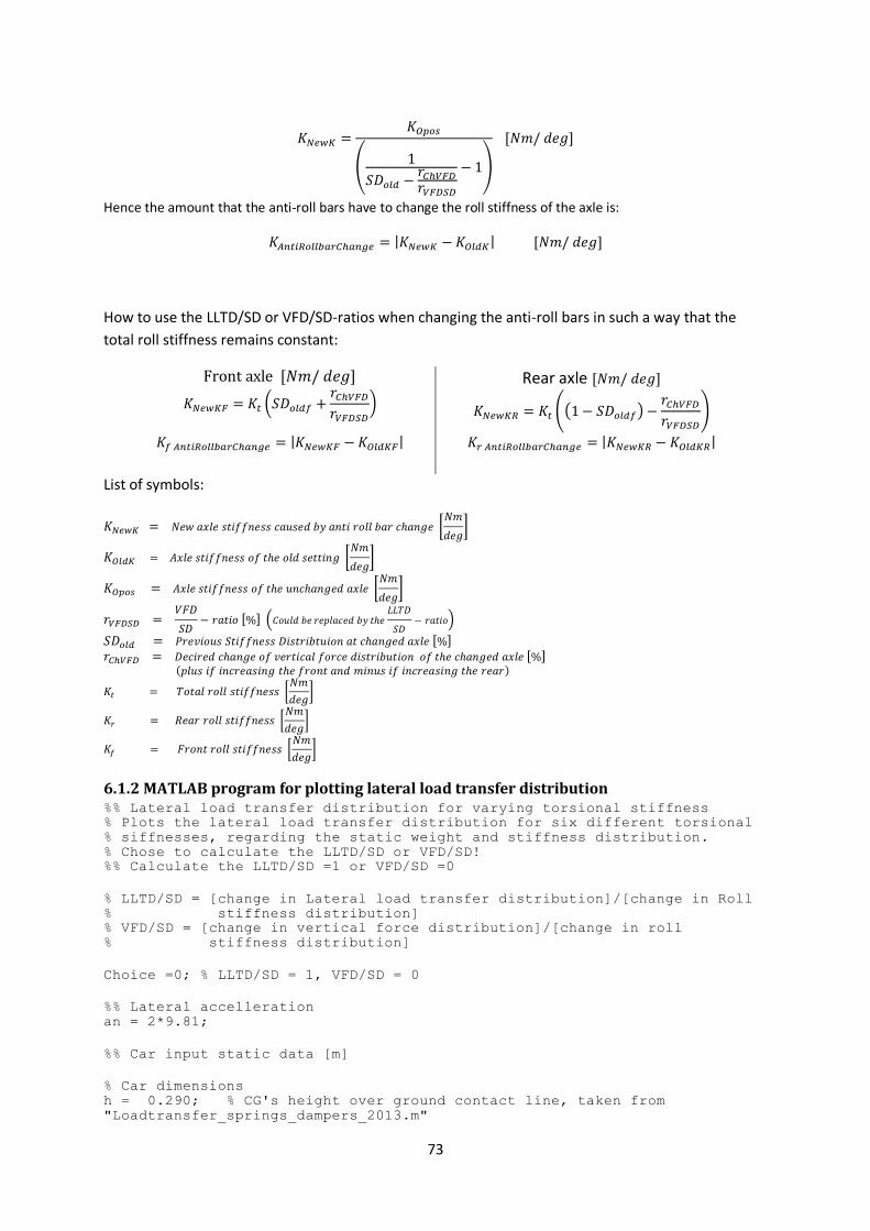
73
𝐾𝑁𝑒𝑤𝐾 =𝐾𝑂𝑝𝑜𝑠
(1
𝑆𝐷𝑜𝑙𝑑 −𝑟𝐶ℎ𝑉𝐹𝐷
𝑟𝑉𝐹𝐷𝑆𝐷
− 1)
[𝑁𝑚/ 𝑑𝑒𝑔]
Hence the amount that the anti-roll bars have to change the roll stiffness of the axle is:
𝐾𝐴𝑛𝑡𝑖𝑅𝑜𝑙𝑙𝑏𝑎𝑟𝐶ℎ𝑎𝑛𝑔𝑒 = |𝐾𝑁𝑒𝑤𝐾 − 𝐾𝑂𝑙𝑑𝐾| [𝑁𝑚/ 𝑑𝑒𝑔]
How to use the LLTD/SD or VFD/SD-ratios when changing the anti-roll bars in such a way that the
total roll stiffness remains constant:
Front axle [𝑁𝑚/ 𝑑𝑒𝑔] Rear axle [𝑁𝑚/ 𝑑𝑒𝑔]
𝐾𝑁𝑒𝑤𝐾𝐹 = 𝐾𝑡 (𝑆𝐷𝑜𝑙𝑑𝑓 +𝑟𝐶ℎ𝑉𝐹𝐷
𝑟𝑉𝐹𝐷𝑆𝐷
) 𝐾𝑁𝑒𝑤𝐾𝑅 = 𝐾𝑡 ((1 − 𝑆𝐷𝑜𝑙𝑑𝑓) −
𝑟𝐶ℎ𝑉𝐹𝐷
𝑟𝑉𝐹𝐷𝑆𝐷
)
𝐾𝑓 𝐴𝑛𝑡𝑖𝑅𝑜𝑙𝑙𝑏𝑎𝑟𝐶ℎ𝑎𝑛𝑔𝑒 = |𝐾𝑁𝑒𝑤𝐾𝐹 − 𝐾𝑂𝑙𝑑𝐾𝐹|
𝐾𝑟 𝐴𝑛𝑡𝑖𝑅𝑜𝑙𝑙𝑏𝑎𝑟𝐶ℎ𝑎𝑛𝑔𝑒 = |𝐾𝑁𝑒𝑤𝐾𝑅 − 𝐾𝑂𝑙𝑑𝐾𝑅|
List of symbols:
𝐾𝑁𝑒𝑤𝐾 = 𝑁𝑒𝑤 𝑎𝑥𝑙𝑒 𝑠𝑡𝑖𝑓𝑓𝑛𝑒𝑠𝑠 𝑐𝑎𝑢𝑠𝑒𝑑 𝑏𝑦 𝑎𝑛𝑡𝑖 𝑟𝑜𝑙𝑙 𝑏𝑎𝑟 𝑐ℎ𝑎𝑛𝑔𝑒 [𝑁𝑚
𝑑𝑒𝑔]
𝐾𝑂𝑙𝑑𝐾 = 𝐴𝑥𝑙𝑒 𝑠𝑡𝑖𝑓𝑓𝑛𝑒𝑠𝑠 𝑜𝑓 𝑡ℎ𝑒 𝑜𝑙𝑑 𝑠𝑒𝑡𝑡𝑖𝑛𝑔 [𝑁𝑚
𝑑𝑒𝑔]
𝐾𝑂𝑝𝑜𝑠 = 𝐴𝑥𝑙𝑒 𝑠𝑡𝑖𝑓𝑓𝑛𝑒𝑠𝑠 𝑜𝑓 𝑡ℎ𝑒 𝑢𝑛𝑐ℎ𝑎𝑛𝑔𝑒𝑑 𝑎𝑥𝑙𝑒 [𝑁𝑚
𝑑𝑒𝑔]
𝑟𝑉𝐹𝐷𝑆𝐷 = 𝑉𝐹𝐷
𝑆𝐷− 𝑟𝑎𝑡𝑖𝑜 [%] (𝐶𝑜𝑢𝑙𝑑 𝑏𝑒 𝑟𝑒𝑝𝑙𝑎𝑐𝑒𝑑 𝑏𝑦 𝑡ℎ𝑒
𝐿𝐿𝑇𝐷
𝑆𝐷− 𝑟𝑎𝑡𝑖𝑜)
𝑆𝐷𝑜𝑙𝑑 = 𝑃𝑟𝑒𝑣𝑖𝑜𝑢𝑠 𝑆𝑡𝑖𝑓𝑓𝑛𝑒𝑠𝑠 𝐷𝑖𝑠𝑡𝑟𝑖𝑏𝑡𝑢𝑖𝑜𝑛 𝑎𝑡 𝑐ℎ𝑎𝑛𝑔𝑒𝑑 𝑎𝑥𝑙𝑒 [%] 𝑟𝐶ℎ𝑉𝐹𝐷 = 𝐷𝑒𝑐𝑖𝑟𝑒𝑑 𝑐ℎ𝑎𝑛𝑔𝑒 𝑜𝑓 𝑣𝑒𝑟𝑡𝑖𝑐𝑎𝑙 𝑓𝑜𝑟𝑐𝑒 𝑑𝑖𝑠𝑡𝑟𝑖𝑏𝑢𝑡𝑖𝑜𝑛 𝑜𝑓 𝑡ℎ𝑒 𝑐ℎ𝑎𝑛𝑔𝑒𝑑 𝑎𝑥𝑙𝑒 [%] (𝑝𝑙𝑢𝑠 𝑖𝑓 𝑖𝑛𝑐𝑟𝑒𝑎𝑠𝑖𝑛𝑔 𝑡ℎ𝑒 𝑓𝑟𝑜𝑛𝑡 𝑎𝑛𝑑 𝑚𝑖𝑛𝑢𝑠 𝑖𝑓 𝑖𝑛𝑐𝑟𝑒𝑎𝑠𝑖𝑛𝑔 𝑡ℎ𝑒 𝑟𝑒𝑎𝑟)
𝐾𝑡 = 𝑇𝑜𝑡𝑎𝑙 𝑟𝑜𝑙𝑙 𝑠𝑡𝑖𝑓𝑓𝑛𝑒𝑠𝑠 [𝑁𝑚
𝑑𝑒𝑔]
𝐾𝑟 = 𝑅𝑒𝑎𝑟 𝑟𝑜𝑙𝑙 𝑠𝑡𝑖𝑓𝑓𝑛𝑒𝑠𝑠 [𝑁𝑚
𝑑𝑒𝑔]
𝐾𝑓 = 𝐹𝑟𝑜𝑛𝑡 𝑟𝑜𝑙𝑙 𝑠𝑡𝑖𝑓𝑓𝑛𝑒𝑠𝑠 [𝑁𝑚
𝑑𝑒𝑔]
6.1.2 MATLAB program for plotting lateral load transfer distribution %% Lateral load transfer distribution for varying torsional stiffness % Plots the lateral load transfer distribution for six different torsional % siffnesses, regarding the static weight and stiffness distribution. % Chose to calculate the LLTD/SD or VFD/SD! %% Calculate the LLTD/SD =1 or VFD/SD =0
% LLTD/SD = [change in Lateral load transfer distribution]/[change in Roll % stiffness distribution] % VFD/SD = [change in vertical force distribution]/[change in roll % stiffness distribution]
Choice =0; % LLTD/SD = 1, VFD/SD = 0 %% Lateral accelleration an = 2*9.81;
%% Car input static data [m] % Car dimensions h = 0.290; % CG's height over ground contact line, taken from
"Loadtransfer_springs_dampers_2013.m"
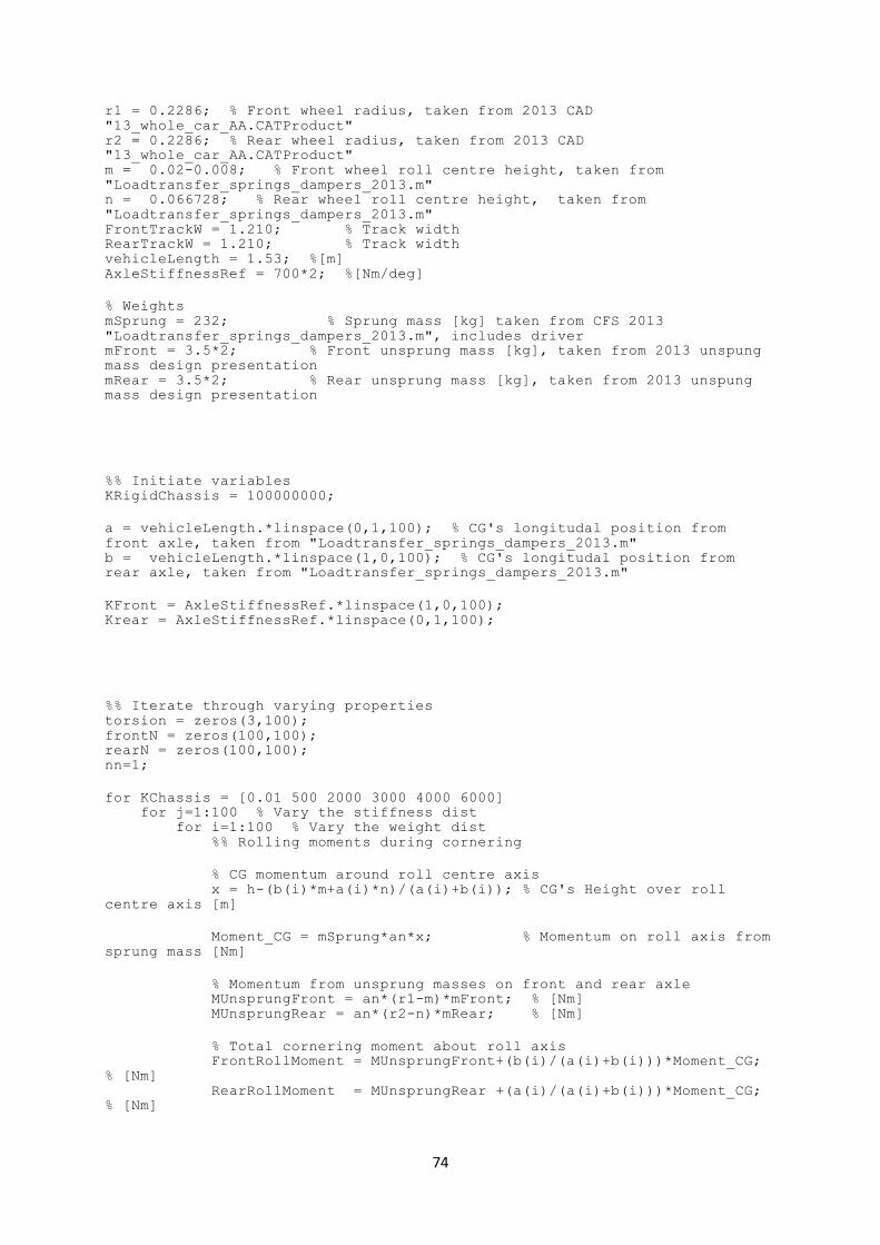
74
r1 = 0.2286; % Front wheel radius, taken from 2013 CAD
"13_whole_car_AA.CATProduct" r2 = 0.2286; % Rear wheel radius, taken from 2013 CAD
"13_whole_car_AA.CATProduct" m = 0.02-0.008; % Front wheel roll centre height, taken from
"Loadtransfer_springs_dampers_2013.m" n = 0.066728; % Rear wheel roll centre height, taken from
"Loadtransfer_springs_dampers_2013.m" FrontTrackW = 1.210; % Track width RearTrackW = 1.210; % Track width vehicleLength = 1.53; %[m] AxleStiffnessRef = 700*2; %[Nm/deg] % Weights mSprung = 232; % Sprung mass [kg] taken from CFS 2013
"Loadtransfer_springs_dampers_2013.m", includes driver mFront = 3.5*2; % Front unsprung mass [kg], taken from 2013 unspung
mass design presentation mRear = 3.5*2; % Rear unsprung mass [kg], taken from 2013 unspung
mass design presentation
%% Initiate variables KRigidChassis = 100000000; a = vehicleLength.*linspace(0,1,100); % CG's longitudal position from
front axle, taken from "Loadtransfer_springs_dampers_2013.m" b = vehicleLength.*linspace(1,0,100); % CG's longitudal position from
rear axle, taken from "Loadtransfer_springs_dampers_2013.m"
KFront = AxleStiffnessRef.*linspace(1,0,100); Krear = AxleStiffnessRef.*linspace(0,1,100);
%% Iterate through varying properties torsion = zeros(3,100); frontN = zeros(100,100); rearN = zeros(100,100); nn=1;
for KChassis = [0.01 500 2000 3000 4000 6000] for j=1:100 % Vary the stiffness dist for i=1:100 % Vary the weight dist %% Rolling moments during cornering
% CG momentum around roll centre axis x = h-(b(i)*m+a(i)*n)/(a(i)+b(i)); % CG's Height over roll
centre axis [m] Moment_CG = mSprung*an*x; % Momentum on roll axis from
sprung mass [Nm]
% Momentum from unsprung masses on front and rear axle MUnsprungFront = an*(r1-m)*mFront; % [Nm] MUnsprungRear = an*(r2-n)*mRear; % [Nm]
% Total cornering moment about roll axis FrontRollMoment = MUnsprungFront+(b(i)/(a(i)+b(i)))*Moment_CG;
% [Nm] RearRollMoment = MUnsprungRear +(a(i)/(a(i)+b(i)))*Moment_CG;
% [Nm]
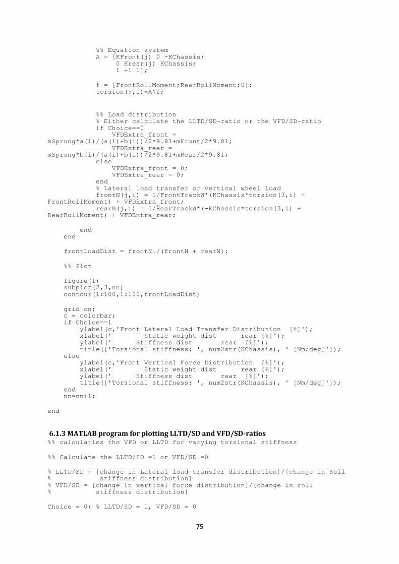
75
%% Equation system A = [KFront(j) 0 -KChassis; 0 Krear(j) KChassis; 1 -1 1];
f = [FrontRollMoment;RearRollMoment;0]; torsion(:,i)=A\f;
%% Load distribution % Either calculate the LLTD/SD-ratio or the VFD/SD-ratio if Choice==0 VFDExtra_front =
mSprung*a(i)/(a(i)+b(i))/2*9.81+mFront/2*9.81; VFDExtra_rear =
mSprung*b(i)/(a(i)+b(i))/2*9.81+mRear/2*9.81; else VFDExtra_front = 0; VFDExtra_rear = 0; end % Lateral load transfer or vertical wheel load frontN(j,i) = 1/FrontTrackW*(KChassis*torsion(3,i) +
FrontRollMoment) + VFDExtra_front; rearN(j,i) = 1/RearTrackW*(-KChassis*torsion(3,i) +
RearRollMoment) + VFDExtra_rear;
end end frontLoadDist = frontN./(frontN + rearN);
%% Plot
figure(1) subplot(2,3,nn) contour(1:100,1:100,frontLoadDist)
grid on; c = colorbar; if Choice==1 ylabel(c,'Front Lateral Load Transfer Distribution [%]'); xlabel(' Static weight dist rear [%]'); ylabel(' Stiffness dist rear [%]'); title(['Torsional stiffness: ', num2str(KChassis), ' [Nm/deg]']); else ylabel(c,'Front Vertical Force Distribution [%]'); xlabel(' Static weight dist rear [%]'); ylabel(' Stiffness dist rear [%]'); title(['Torsional stiffness: ', num2str(KChassis), ' [Nm/deg]']); end nn=nn+1;
end
6.1.3 MATLAB program for plotting LLTD/SD and VFD/SD-ratios %% calculaties the VFD or LLTD for varying torsional stiffness
%% Calculate the LLTD/SD =1 or VFD/SD =0 % LLTD/SD = [change in Lateral load transfer distribution]/[change in Roll % stiffness distribution] % VFD/SD = [change in vertical force distribution]/[change in roll % stiffness distribution]
Choice = 0; % LLTD/SD = 1, VFD/SD = 0
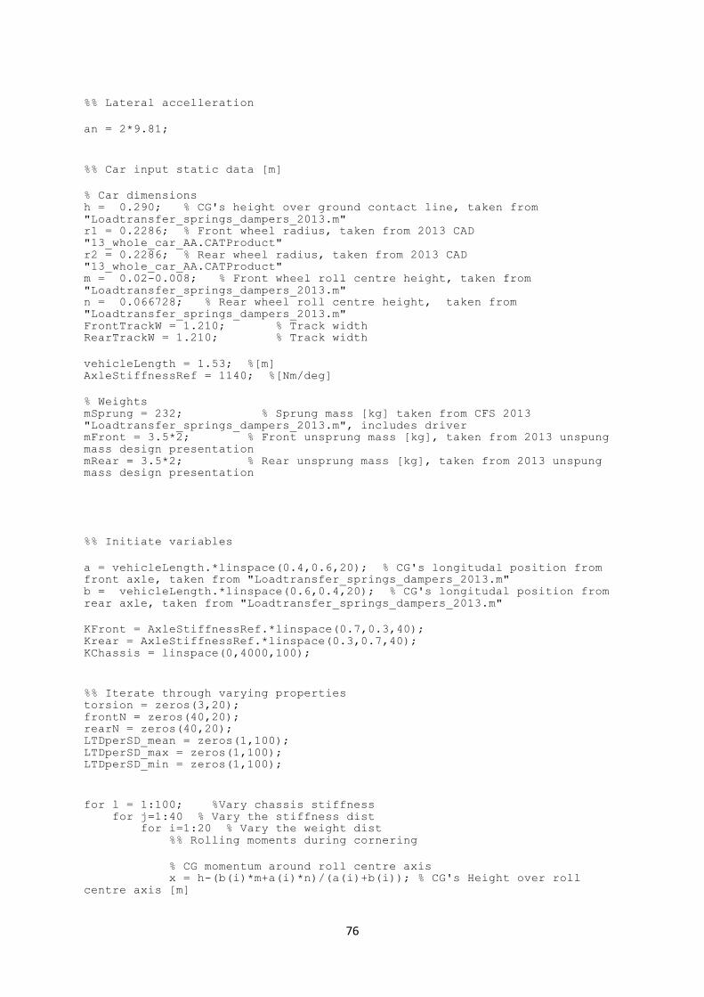
76
%% Lateral accelleration
an = 2*9.81;
%% Car input static data [m] % Car dimensions h = 0.290; % CG's height over ground contact line, taken from
"Loadtransfer_springs_dampers_2013.m" r1 = 0.2286; % Front wheel radius, taken from 2013 CAD
"13_whole_car_AA.CATProduct" r2 = 0.2286; % Rear wheel radius, taken from 2013 CAD
"13_whole_car_AA.CATProduct" m = 0.02-0.008; % Front wheel roll centre height, taken from
"Loadtransfer_springs_dampers_2013.m" n = 0.066728; % Rear wheel roll centre height, taken from
"Loadtransfer_springs_dampers_2013.m" FrontTrackW = 1.210; % Track width RearTrackW = 1.210; % Track width
vehicleLength = 1.53; %[m] AxleStiffnessRef = 1140; %[Nm/deg] % Weights mSprung = 232; % Sprung mass [kg] taken from CFS 2013
"Loadtransfer_springs_dampers_2013.m", includes driver mFront = 3.5*2; % Front unsprung mass [kg], taken from 2013 unspung
mass design presentation mRear = 3.5*2; % Rear unsprung mass [kg], taken from 2013 unspung
mass design presentation
%% Initiate variables
a = vehicleLength.*linspace(0.4,0.6,20); % CG's longitudal position from
front axle, taken from "Loadtransfer_springs_dampers_2013.m" b = vehicleLength.*linspace(0.6,0.4,20); % CG's longitudal position from
rear axle, taken from "Loadtransfer_springs_dampers_2013.m" KFront = AxleStiffnessRef.*linspace(0.7,0.3,40); Krear = AxleStiffnessRef.*linspace(0.3,0.7,40); KChassis = linspace(0,4000,100);
%% Iterate through varying properties torsion = zeros(3,20); frontN = zeros(40,20); rearN = zeros(40,20); LTDperSD_mean = zeros(1,100); LTDperSD_max = zeros(1,100); LTDperSD_min = zeros(1,100);
for l = 1:100; %Vary chassis stiffness for j=1:40 % Vary the stiffness dist for i=1:20 % Vary the weight dist %% Rolling moments during cornering
% CG momentum around roll centre axis x = h-(b(i)*m+a(i)*n)/(a(i)+b(i)); % CG's Height over roll
centre axis [m]
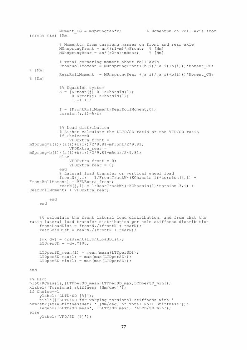
77
Moment_CG = mSprung*an*x; % Momentum on roll axis from
sprung mass [Nm]
% Momentum from unsprung masses on front and rear axle MUnsprungFront = an*(r1-m)*mFront; % [Nm] MUnsprungRear = an*(r2-n)*mRear; % [Nm]
% Total cornering moment about roll axis FrontRollMoment = MUnsprungFront+(b(i)/(a(i)+b(i)))*Moment_CG;
% [Nm] RearRollMoment = MUnsprungRear +(a(i)/(a(i)+b(i)))*Moment_CG;
% [Nm]
%% Equation system A = [KFront(j) 0 -KChassis(l); 0 Krear(j) KChassis(l); 1 -1 1];
f = [FrontRollMoment;RearRollMoment;0]; torsion(:,i)=A\f;
%% Load distribution % Either calculate the LLTD/SD-ratio or the VFD/SD-ratio if Choice==0 VFDExtra_front =
mSprung*a(i)/(a(i)+b(i))/2*9.81+mFront/2*9.81; VFDExtra_rear =
mSprung*b(i)/(a(i)+b(i))/2*9.81+mRear/2*9.81; else VFDExtra_front = 0; VFDExtra_rear = 0; end % Lateral load transfer or vertical wheel load frontN(j,i) = 1/FrontTrackW*(KChassis(l)*torsion(3,i) +
FrontRollMoment) + VFDExtra_front; rearN(j,i) = 1/RearTrackW*(-KChassis(l)*torsion(3,i) +
RearRollMoment) + VFDExtra_rear;
end end
%% calculate the front lateral load distribution, and from that the
ratio lateral load transfer distribution per axle stiffness distribution frontLoadDist = frontN./(frontN + rearN); rearLoadDist = rearN./(frontN + rearN);
[dx dy] = gradient(frontLoadDist); LTDperSD = -dy.*100;
LTDperSD_mean(l) = mean(mean(LTDperSD)); LTDperSD_max(l) = max(max(LTDperSD)); LTDperSD_min(l) = min(min(LTDperSD));
end
%% Plot plot(KChassis,[LTDperSD_mean;LTDperSD_max;LTDperSD_min]); xlabel('Torsional stiffness [Nm/deg]'); if Choice==1 ylabel('LLTD/SD [%]'); title(['LLTD/SD for varying torsional stiffness with '
num2str(AxleStiffnessRef) ' [Nm/deg] of Total Roll Stiffness']); legend('LLTD/SD mean', 'LLTD/SD max', 'LLTD/SD min'); else ylabel('VFD/SD [%]');
78
title(['VFD/SD for varying torsional stiffness with'
num2str(AxleStiffnessRef) ' [Nm/deg] of Total Roll Stiffness']); legend('VFD/SD mean', 'VFD/SD max', 'VFD/SD min'); end grid on;
6.1.4 MATLAB program for calculation of the total roll stiffness impact clc; clear all; close all; %% Calculate the LLTD/SD =1 or VFD/SD =0 % LLTD/SD = [change in Lateral load transfer distribution]/[change in Roll % stiffness distribution] % VFD/SD = [change in vertical force distribution]/[change in roll % stiffness distribution]
Choice = 0; % LLTD/SD = 1, VFD/SD = 0
%% Lateral accelleration an = 2*9.81;
%% Car input static data [m]
% Car dimensions h = 0.40; % CG's height over ground contact line, taken from
"Loadtransfer_springs_dampers_2013.m" r1 = 0.2286; % Front wheel radius, taken from 2013 CAD
"13_whole_car_AA.CATProduct" r2 = 0.2286; % Rear wheel radius, taken from 2013 CAD
"13_whole_car_AA.CATProduct" m = 0.02-0.008; % Front wheel roll centre height, taken from
"Loadtransfer_springs_dampers_2013.m" n = 0.066728; % Rear wheel roll centre height, taken from
"Loadtransfer_springs_dampers_2013.m" FrontTrackW = 1.210; % Track width RearTrackW = 1.210; % Track width vehicleLength = 1.53; %[m]
% Weights mSprung = 232; % Sprung mass [kg] taken from CFS 2013
"Loadtransfer_springs_dampers_2013.m", includes driver mFront = 3.5*2; % Front unsprung mass [kg], taken from 2013 unspung
mass design presentation mRear = 3.5*2; % Rear unsprung mass [kg], taken from 2013 unspung
mass design presentation
%% Initiate variables of car properties a = vehicleLength.*linspace(0.4,0.6,20); % CG's longitudal position from
front axle, taken from "Loadtransfer_springs_dampers_2013.m" b = vehicleLength.*linspace(0.6,0.4,20); % CG's longitudal position from
rear axle, taken from "Loadtransfer_springs_dampers_2013.m" KChassis = linspace(0,20000,100); AxleStiffnessRef = linspace(100,2500,20); %[Nm/deg] %% Iterate through varying properties torsion = zeros(3,20); frontN = zeros(40,20);
79
rearN = zeros(40,20); LTDperSD_mean = zeros(1,100); LTDperSD_max = zeros(1,100); LTDperSD_min = zeros(1,100); torsional_stiffness = zeros(5,20);
for k = 1:20; % vary the axlestiffness KFront = AxleStiffnessRef(k).*linspace(0.7,0.3,40); Krear = AxleStiffnessRef(k).*linspace(0.3,0.7,40);
for l = 1:100; %Vary chassis stiffness for j=1:40 % Vary the stiffness dist for i=1:20 % Vary the weight dist %% Rolling moments during cornering
% CG momentum around roll centre axis x = h-(b(i)*m+a(i)*n)/(a(i)+b(i)); % CG's Height over roll
centre axis [m] Moment_CG = mSprung*an*x; % Momentum on roll axis
from sprung mass [Nm]
% Momentum from unsprung masses on front and rear axle MUnsprungFront = an*(r1-m)*mFront; % [Nm] MUnsprungRear = an*(r2-n)*mRear; % [Nm]
% Total cornering moment about roll axis FrontRollMoment =
MUnsprungFront+(b(i)/(a(i)+b(i)))*Moment_CG; % [Nm] RearRollMoment = MUnsprungRear
+(a(i)/(a(i)+b(i)))*Moment_CG; % [Nm]
%% Equation system A = [KFront(j) 0 -KChassis(l); 0 Krear(j) KChassis(l); 1 -1 1];
f = [FrontRollMoment;RearRollMoment;0]; torsion(:,i)=A\f;
%% Load distribution % Either calculate the LLTD/SD-ratio or the VFD/SD-ratio if Choice==0 VFDExtra_front =
mSprung*a(i)/(a(i)+b(i))/2*9.81+mFront/2*9.81; VFDExtra_rear =
mSprung*b(i)/(a(i)+b(i))/2*9.81+mRear/2*9.81; else VFDExtra_front = 0; VFDExtra_rear = 0; end % Lateral load transfer or vertical wheel load frontN(j,i) = 1/FrontTrackW*(KChassis(l)*torsion(3,i) +
FrontRollMoment) + VFDExtra_front; rearN(j,i) = 1/RearTrackW*(-KChassis(l)*torsion(3,i) +
RearRollMoment) + VFDExtra_rear;
end end
%% calculate the front lateral load distribution, and from that the
ratio lateral load transfer distribution per axle stiffness distribution frontLoadDist = frontN./(frontN + rearN);
[dx dy] = gradient(frontLoadDist); LTDperSD = -dy.*100;

80
LTDperSD_mean(l) = mean(mean(LTDperSD)); LTDperSD_max(l) = max(max(LTDperSD)); LTDperSD_min(l) = min(min(LTDperSD)); end % Picks out 50, 60, 70, 80, and 90 % of VFD or LLTD if Choice==1 torsional_stiffness(:,k) = [KChassis(find(LTDperSD_min>=0.5 ,1));
KChassis(find(LTDperSD_min>=0.60 ,1)); KChassis(find(LTDperSD_min>=0.7
,1)); KChassis(find(LTDperSD_min>=0.8 ,1));
KChassis(find(LTDperSD_min>=0.9 ,1))]; else torsional_stiffness(:,k) = [KChassis(find(LTDperSD_min>=0.2 ,1));
KChassis(find(LTDperSD_min>=0.3 ,1)); KChassis(find(LTDperSD_min>=0.4 ,1));
KChassis(find(LTDperSD_min>=0.45 ,1)); KChassis(find(LTDperSD_min>=0.50
,1))]; end end
%% Plot for i = 1:5 koefficent(i) =
mean((torsional_stiffness(i,5:length(torsional_stiffness)))./(AxleStiffness
Ref(5:length(torsional_stiffness)))); end
%plot(torsional_stiffness,AxleStiffnessRef); %hold on plot((koefficent'*AxleStiffnessRef),AxleStiffnessRef) xlabel('Torsional stiffness [Nm/deg]'); ylabel('Total roll stiffness [Nm/deg]'); if Choice==1 legend('LLTD/SD 50 %', 'LLTD/SD 60%', 'LLTD/SD 70%', 'LLTD/SD 80%',
'LLTD/SD 90%'); title('Torsional stiffness satisfying different LLTD/SD ratios'); else legend('VFD/SD 20 %', 'VFD/SD 30%', 'VFD/SD 40%', 'VFD/SD 45%', 'VFD/SD
50%'); title('Torsional stiffness satisfying different VFD/SD ratios'); end grid on; axis([0 4000 0 2500])