analysis and modeling of urban land cover change in ... · analysis and modeling of urban land...

Remote Sens. 2010, 2, 1549-1563; doi:10.3390/rs2061549

Remote Sensing ISSN 2072-4292

www.mdpi.com/journal/remotesensing

Article

Analysis and Modeling of Urban Land Cover Change in Setúbal

and Sesimbra, Portugal

Yikalo H. Araya 1,*

and Pedro Cabral

2

1 Department of Geography, York University, 4700 Keele street, M3J 1P3, TO, Canada

2 Instituto Superior de Estatística e Gestão de Informação, ISEGI, Universidade Nova de Lisboa,

1070-312 LISBOA, Portugal; E-Mail: [email protected]

* Author to whom correspondence should be addressed; E-Mail: [email protected];

Tel.: +1-416-736-2100 ext. 66187.

Received: 24 March 2010; in revised form: 31 May 2010 / Accepted: 2 June 2010 /

Published: 9 June 2010

Abstract: The expansion of cities entails the abandonment of forest and agricultural lands,

and these lands‘ conversion into urban areas, which results in substantial impacts on

ecosystems. Monitoring these changes and planning urban development can be

successfully achieved using multitemporal remotely sensed data, spatial metrics, and

modeling. In this paper, urban land use change analysis and modeling was carried out for

the Concelhos of Setúbal and Sesimbra in Portugal. An existing land cover map for the

year 1990, together with two derived land cover maps from multispectral satellite images

for the years 2000 and 2006, were utilized using an object-oriented classification approach.

Classification accuracy assessment revealed satisfactory results that fulfilled minimum

standard accuracy levels. Urban land use dynamics, in terms of both patterns and

quantities, were studied using selected landscape metrics and the Shannon Entropy index.

Results show that urban areas increased by 91.11% between 1990 and 2006. In contrast,

the change was only 6.34% between 2000 and 2006. The entropy value was 0.73 for both

municipalities in 1990, indicating a high rate of urban sprawl in the area. In 2006, this

value, for both Sesimbra and Setúbal, reached almost 0.90. This is demonstrative of a

tendency toward intensive urban sprawl. Urban land use change for the year 2020 was

modeled using a Cellular Automata based approach. The predictive power of the model

was successfully validated using Kappa variations. Projected land cover changes show a

growing tendency in urban land use, which might threaten areas that are currently reserved

for natural parks and agricultural lands.

OPEN ACCESS

Remote Sens. 2010, 2

1550

Keywords: object-oriented image classification; change detection, landscape metrics; land

cover change modeling

1. Introduction

The history of urban growth indicates that urban areas are one of most dynamic places on the

Earth‘s surface. Despite its regional economic importance, urban growth has a considerable impact on

the surrounding ecosystem [1]. Most often, the trend of urban growth is towards the urban-rural-fringe,

where there is less built-up area, and access to irrigation and other water management systems. In the

last few decades, a substantial growth of urban areas has occurred worldwide. Population increase is

one of the most obvious agents responsible for this growth. In 1900, only 14% of the world‘s

population lived in urban areas, but by 2000, this figure had increased to 47% [2]. The report also

predicts that by 2030, the percentage of the population residing in urban areas will be 60%. Currently,

the major environmental concerns that have to be analyzed and monitored carefully, for effective land

use management, are those driven by urban growth.

Effective analysis and monitoring of land cover changes require a substantial amount of data about

the Earth‘s surface. This is most widely achieved by using remote sensing (RS) tools. Remote sensing

provides an excellent source of data, from which updated land use/land cover (LULC) information and

changes can be extracted, analyzed, and simulated efficiently. LULC mapping, derived from remotely

sensed data, has long been an area of focus for various researchers [3]; recent advances in Geographic

information systems (GIS) and RS tools and methods enable researchers to model urban growth

effectively. Cellular Automata (CA) constitutes a possible approach to urban growth modeling by

simulating spatial processes as discrete and dynamic systems in space and time that operate on a

uniform grid-based space [4,5]. The ability of CA to represent complex systems with spatio-temporal

behavior, from a small set of simple rules and states, makes it suitable for modeling and investigating

urban environments [4]. Planning activities may also benefit from CA; CA enables the understanding

of the urbanization phenomenon and the exploration of what-if scenarios.

In this study, an integrated approach incorporating GIS, RS, and modeling is applied to identify and

analyze patterns of urban changes within the Setúbal and Sesimbra municipalities between the years

1990 and 2006. The study also aims to determine the probable future developed areas so as to enable

the anticipation of planning policies that aim to preserve the unique natural characteristics of the

study area.

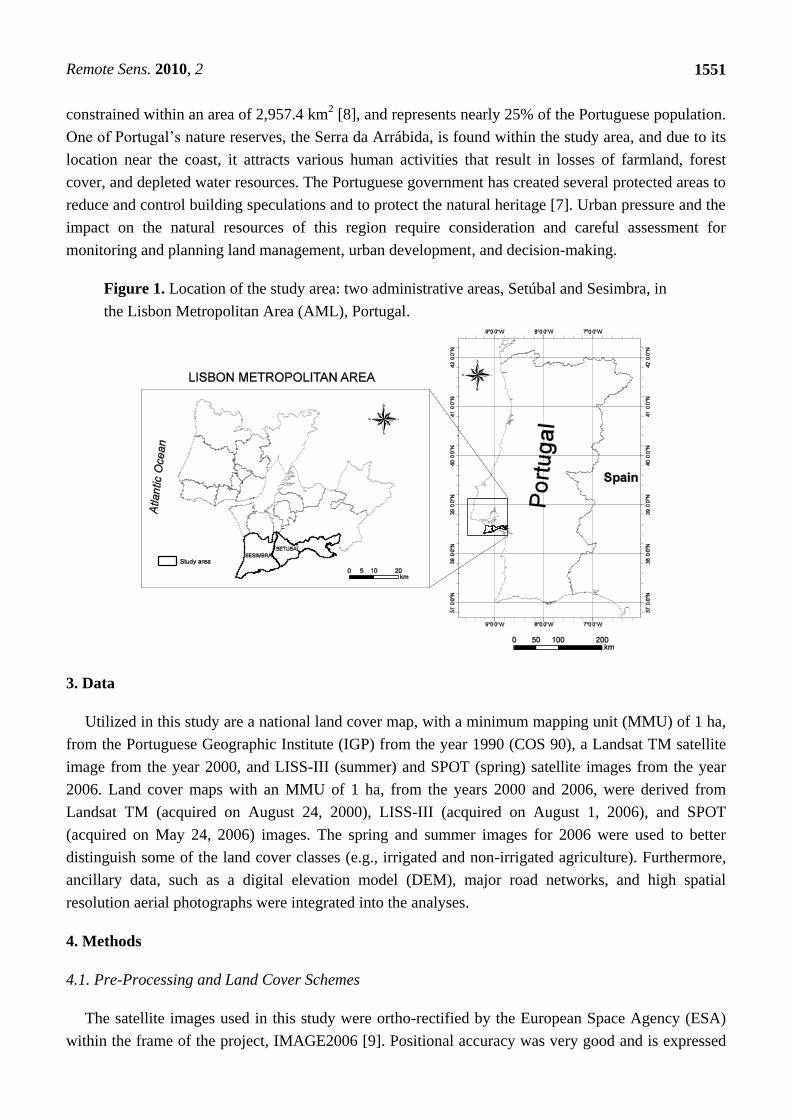
2. Study Area

The study focuses on two administrative areas, Setúbal and Sesimbra, in the Lisbon Metropolitan

Area (AML), Portugal (Figure 1).

The AML has experienced considerable population growth in two distinct phases: the rural to urban

migration, which took place from 1940 to 1960, and the return of thousands of Portuguese from the

overseas ex-colonies in the 1970s [6,7]. These phases significantly affected the rate of urban sprawl in

the area and led to a current population in the AML of approximately 2.6 million. The population is


1551

constrained within an area of 2,957.4 km2 [8], and represents nearly 25% of the Portuguese population.

One of Portugal‘s nature reserves, the Serra da Arrábida, is found within the study area, and due to its

location near the coast, it attracts various human activities that result in losses of farmland, forest

cover, and depleted water resources. The Portuguese government has created several protected areas to

reduce and control building speculations and to protect the natural heritage [7]. Urban pressure and the

impact on the natural resources of this region require consideration and careful assessment for

monitoring and planning land management, urban development, and decision-making.

Figure 1. Location of the study area: two administrative areas, Setúbal and Sesimbra, in

the Lisbon Metropolitan Area (AML), Portugal.

3. Data

Utilized in this study are a national land cover map, with a minimum mapping unit (MMU) of 1 ha,

from the Portuguese Geographic Institute (IGP) from the year 1990 (COS 90), a Landsat TM satellite

image from the year 2000, and LISS-III (summer) and SPOT (spring) satellite images from the year

2006. Land cover maps with an MMU of 1 ha, from the years 2000 and 2006, were derived from

Landsat TM (acquired on August 24, 2000), LISS-III (acquired on August 1, 2006), and SPOT

(acquired on May 24, 2006) images. The spring and summer images for 2006 were used to better

distinguish some of the land cover classes (e.g., irrigated and non-irrigated agriculture). Furthermore,

ancillary data, such as a digital elevation model (DEM), major road networks, and high spatial

resolution aerial photographs were integrated into the analyses.

4. Methods

4.1. Pre-Processing and Land Cover Schemes

The satellite images used in this study were ortho-rectified by the European Space Agency (ESA)

within the frame of the project, IMAGE2006 [9]. Positional accuracy was very good and is expressed


1552

with a root mean square error of less than 1 pixel. As a pre-processing phase, individual bands were

extracted for further processing and analysis to cover the entire study area. Two scenes of spring

images for the year 2006 were spliced together on a band by band basis because no single scene

covered the entire study area. The datasets were provided along with a 44 land cover class legend. For

the sake of simplicity, the 44 classes were aggregated into seven major classes, as shown in Table 1.

Table 1. Land cover classes used in the study.

Land cover classes Descriptions based on the CORINE land cover classes

Built-up areas All forms of urban fabrics and urban related features

Urban vegetation Urban vegetation or urban parks, or both

Non-irrigated Annual and permanent crops, complex cultivation patterns, and agriculture

with natural vegetation

Irrigated land Permanently irrigated land, rice fields, and fruit plantations

Forest cover Deciduous, coniferous, mixed forest, and transitional woodland/shrub

Bare land Sand plains and dunes, and bare rock

Water bodies Water courses, water bodies, estuaries, and salt marshes

4.2. Land Cover Classification and Accuracy Assessment

The advent of satellite data in the last few decades opened up a new dimension for the generation of

land cover information. While the extraction of such information is possible using the ‗traditional‘

approaches of surveying or digitizing, land cover information extraction that is based on image

classification has attracted the attention of many remote sensing researchers [10]. The latter is now

considered the ‗standard‘ approach [11]. In various empirical studies, different classification

techniques have been discussed and they can be categorized as being either supervised or

un-supervised; parametric or non-parametric; hard or soft classifiers [10]. All classifiers have

limitations, but alternative methods can be suggested to deal with those limitations. A supervised

pixel-based technique is, for example, criticized for producing inconsistent ―salt and pepper‖ output.

An alternative object-oriented technique has been suggested for a better and more cohesive

classification result. This is because the world is not ―pixelated‖; rather it is arranged in objects [12].

Such object-based classifiers are essential for urban land change studies [13] because of the

heterogeneous nature of urban areas.

We utilized eCognition software, an object-oriented image analysis program, to classify the satellite

images. Land cover classification in eCognition is based on the process of image segmentation, where

pixels are merged into objects based on the pixel‘s spectral properties and the defined scale

parameters. Scale parameters refer to the average size of image objects. The segmentation process

stops when the image objects exceeds a user-defined threshold [14]. Image segmentation in eCognition

requires some parameters to be set: (1) image layer weights: indicate the importance of a layer; (2)

scale parameter; (3) color: determines the homogeneity of the image; and (4) shape: controls the

degree of object shape homogeneity. There is no specific guideline on the rules to be set and these

parameters are often set in a trial and error mode. In this case, all the image layers were considered and

given equal importance (i.e., 1). Additionally, different scale parameters, based on visual analysis of

segmentation results, were attempted. Once the segmentation process was done, classification was


1553

implemented using a resource-based sample collection and a standard nearest neighbor algorithm.

Based on these procedures, land cover maps for the years 2000 and 2006 were generated.

Accuracy assessment, which is an integral part of any image classification process, was calculated to

estimate the accuracy of the land cover classifications. A confusion matrix is the common way of

representing classification; this has been recommended and adopted as the standard reporting

convention [15]. In this paper, accuracy assessment was achieved using a high spatial resolution (50 cm)

aerial photograph as reference. A set of reference points (240 stratified random points) were generated

for each derived map. These points were verified and labeled against the reference data. The overall

user‘s and producer‘s accuracies were calculated from the matrices. The Kappa coefficient, [16],

which is one of the most popular measures of addressing the difference between actual agreement and

chance agreement, was also computed.

4.3. Landscape Metrics and Urban Sprawl Measurement

4.3.1. Landscape Metrics

Changes in urban structures can be described using information obtained from spatial metrics,

which are algorithms used to describe and quantify the spatial characteristics of patches, class areas,

and the entire landscape [17,18]. The changes in urban landscape were measured and analyzed using

the FRAGSTATS tool and thematic maps that represent both built-up and non-built-up patches. In this

paper, seven spatial metrics (CA, NP, ED, LPI, EMN_MN, FRAC_AM, and Contagion) were used for

analyzing urban land cover changes (Table 2). The selection of the metrics was based on their

simplicity and effectiveness in depicting urban forms evolution, as demonstrated in previous

researches [17-21].

Table 2. Spatial metrics used in the study.

Metrics Description Units Range

CA-Class Area CA measures total areas of built-up and non-built-up

areas in the landscape in hectares

Hectares CA>0, no limit

NP-Number of Patches NP is the number of built-up and non-built-up patches in

the landscape

None NP≥0, no limit

ED-Edge Density ED equals the sum of the lengths (m) of all edge

segments involving the patch type, divided by the total

landscape area (m2)

Meters per

hectare

ED≥0, no limit

LPI-Largest Patch Index LPI percentage of the landscape comprised by the

largest patch

Percent 0<LIP≤100

EMN_MN- Euclidian Mean

Nearest Neighbor Distance

Equals the distance (m) to the nearest neighboring patch

of the same

type, based on the shortest edge-to-edge distance

Meters EMN_MN>0, no

limit


1554

Table 2. Cont.

FRAC_AM: Area

weighted mean patch

fractal dimension

Area weighted mean value of the fractal dimension values of all

urban patches; the fractal dimension of a patch equals two times

the logarithm of patch area (m2), while the perimeter is adjusted

to correct for its raster bias

None 1≤FRAC_AM≤2

Contagion Describes the heterogeneity of a landscape and measures the

extent to which landscapes are aggregated or clumped

Percent 0<Contagion≤100

4.3.2. Urban Sprawl Measurement Using Shannon Entropy

Urban sprawl is a complex phenomenon and has both environmental and social impacts [22,23]. It

can be caused by population growth, topography, proximity to major resources, services, and

infrastructure. Many attempts have been made to measure urban sprawl [23-25] by measuring

Shannon‘s Entropy within a GIS. Shannon‘s Entropy is used to measure the degree of spatial

concentration and dispersion, as defined by geographical variables [24-26]. The entropy value varies

from 0 to 1. If the distribution is maximally concentrated in one region, the lowest entropy value (i.e.,

0) is obtained, while an evenly dispersed distribution across space gives a maximum value of 1. In this

study, urban sprawl, over a period from 1990 to 2006, was determined by computing built-up areas

from land cover maps of the years 1990, 2000, and 2006. Afterwards, Shannon entropy calculations

were made. The relative entropy (En) is given by,

where , and xi is the density of land development, which equals the amount of built-up

land divided by the total amount of land in the ith

of n total zones. The number of zones, in this paper,

refers the number of buffers around the city center. In this study, 15 and 16 km concentric buffer rings

around the city centers of the two areas were needed to cover all parts of Setúbal and

Sesimbra, respectively.

4.4. Urban Land Use Change Modeling Using CA-Markov

4.4.1. CA-Markov Model Description

This study adopts an existing modeling technique, CA-Markov Chain analysis, embedded in IDRISI

Kilimanjaro software from Clarks Labs. A Markov Chain CA integrates two techniques: Markov

Chain analysis and CA. The Markov Chain analysis describes the probability of land cover change

from one period to another by developing a transition probability matrix between t1 and t2. The

probabilities may be accurate on a per category basis, but there is no knowledge of the spatial

distribution of occurrences within each land cover class [27]. In order to add the spatial character to the

model, CA is integrated into the Markovian approach. The CA component of the CA-Markov model

allows the transition probabilities of one pixel to be a function of the neighboring pixels. CA-Markov

models the change of several classes of cells by using a Markov transition matrix; a suitability map and

a neighborhood filter [27].


1555

In this study, the Markov Chain analysis model was implemented using the Markov module

available in the software. The first step in the model was to develop a transition probability matrix for

each of the land cover classes between the years 1990 and 2000, and this in turn was used as an input

for modeling land cover change. In addition, two types of criteria (constraints and factors) were

developed to determine which lands were to be considered for further development (suitable lands).

The constraints were standardized into a Boolean character of 0 and 1, while the factors were

standardized to a continuous scale of suitability from 0 (least suitable) to 255 (most suitable). The

constraints included water bodies, existing urban areas, and natural parks (Table 3). These constraints

were standardized into continuous variables by applying Sigmoidal, J-shaped, and Linear functions.

Details of these fuzzy scaling approaches can be found in [27]. A transition suitability image collection

was created using the suitability maps derived from the two criteria using the scaling approaches. The

decision rules used to generate the criteria and factors were based on the legislation defined by [28].

Table 3. Boolean approach criteria development.

Change Drivers Descriptions

Land cover Based on the trend of the land cover change; agricultural land and bare lands are

considered the two possible land cover types available for development.

Distance from roads Areas within 500 m of major road networks are considered suitable [29]. Thus, the

continuous image of distance from roads was reclassified to a Boolean expression such

that areas within 500 m of the road are suitable.

Slope Areas that have low slopes (less than 15%) are suitable for development while areas with

greater than 15% slope are not suitable

Distance from water bodies A protection buffer of 50 m from the sea and navigable waters was created and areas

within 50 m of the water bodies were considered unsuitable.

Distance from built-up areas Areas close to developed areas are more suitable for urban development than areas far

from built-up areas.

Distance from protected areas To preserve the natural park, a protection zone of 50 m is stated in the legislations, and

areas within 50 m of the protected areas are considered unsuitable.

4.4.2. Implementing and Validating the Model

CA analysis was carried out with the CA-Markov module, which uses the output from the above

stated Markov Chain analysis and transition suitability image collection, and applies a contiguity filter.

The Markov module is based on the first law of Geography by using a contiguity rule [30]. The rule

states that a pixel that is near one specific land cover category (e.g., urban areas) is more likely to

become that category than a pixel that is farther. The definition of nearby is determined by a spatial

filter that the user specifies. In this study, a contiguity filter of 5 × 5 pixels was applied.

Model validation is an important step in the modeling process although there is no consensus on the

criteria to assess the performance of land use change models [31]. One way to quantify the predictive

power of the model is to compare the result of the simulation t2 (2006) to a reference or ―real‖ map of

t2 (2006) using Kappa variations [31,32]: Kappa for no information (Kno), Kappa for location (Klocation),

and Kappa for quantity (Kquantity). Kno indicates the proportion classified correctly relative to the

expected proportion classified correctly by a simulation with no ability to specify accurately quantity

or location [31]. Klocation is defined as the success due to a simulation‘s ability to specify location


1556

divided by the maximum possible success due to a simulation‘s ability to specify location

perfectly [31]. Kquantity is a measure of validation of the simulations to predict quantity perfectly. If the

predictive power of a model is considered strong (i.e., greater than 80%), then it will be reasonable to

make future projections (i.e., in this case for year 2020) assuming that the transition mechanism

verified between 1990 and 2000 is going to be repeated.

5. Results and Discussions

5.1. Land Cover Classification and Accuracy Assessment

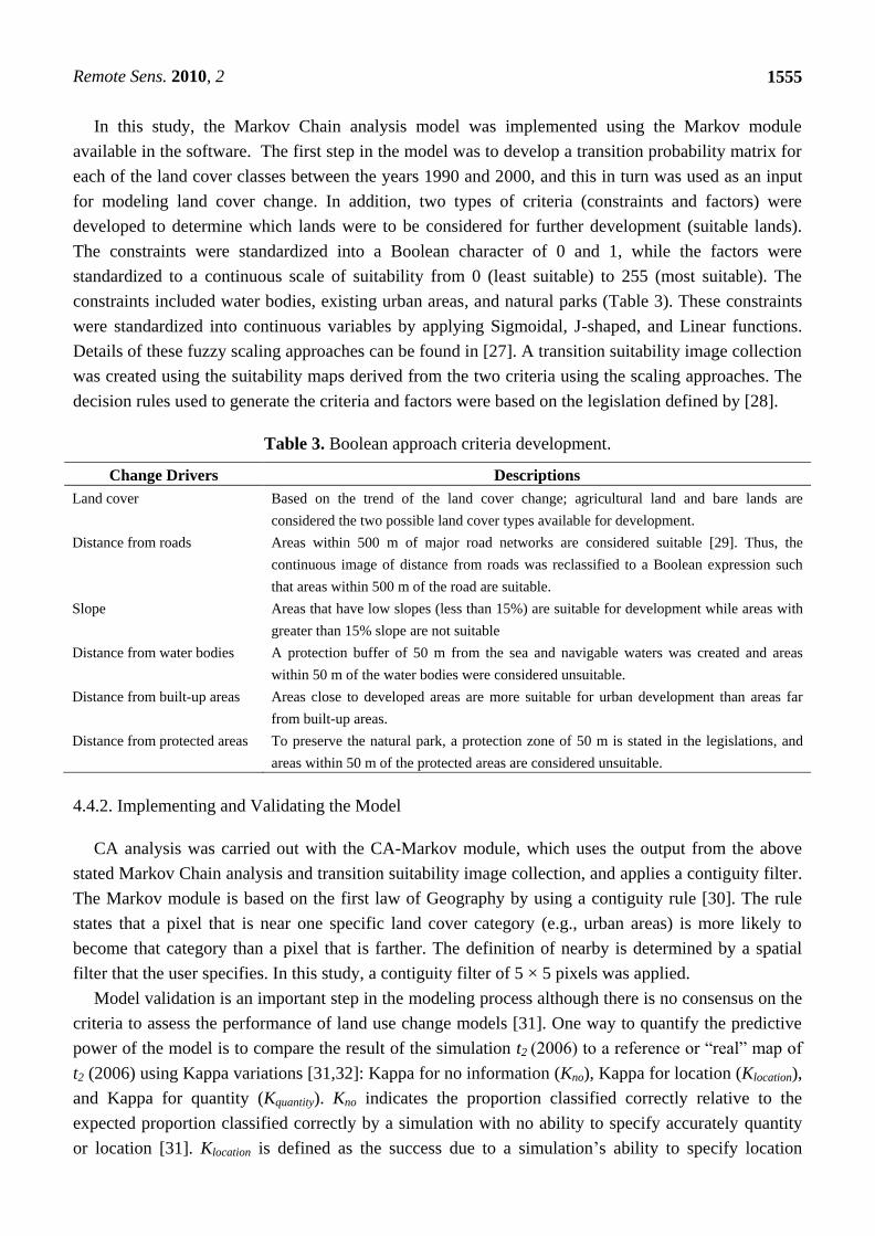
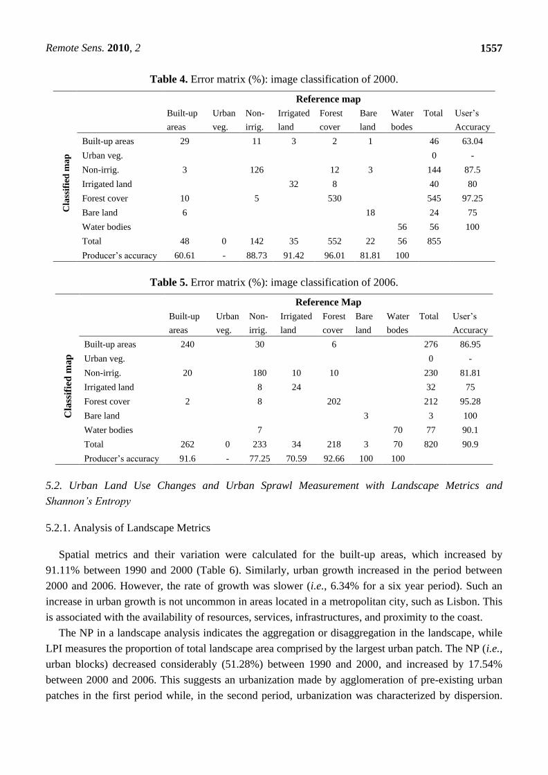
An object-oriented image analysis was applied to derive the LULC maps (Figure 2). In order to use

the derived maps for further change analysis, the errors were evaluated and quantified in terms of

classification accuracy (Tables 4 and 5). Overall accuracies for the maps of 2000 and 2006 were,

respectively, 92.51% and 87.68%. In [33], it is noted that a minimum accuracy value of 85% is

required for effective and reliable land cover change analysis and modeling. The classification

achieved in this study produces an overall accuracy that fulfils the minimum accuracy threshold.

However, looking at Table 4, the user‘s and producer‘s accuracies of the urban class, which is the class

of most interest in this study, provide accuracies of 63.04% and 60.61%, respectively. In other words,

only 60.61% of the urban areas have been correctly identified as urban and only 63.04% of the areas

classified as urban are actually urban. A more careful look at the error matrix reveals that there is

significant confusion in discriminating urban areas from non-irrigated land. The user‘s and producer‘s

accuracies for the urban category in Table 5 are greater than 85%, which are sensible measures of

accuracy. It is important to note that the user‘s and producer‘s accuracy are sensitive to a number of

factors, including the number of random points generated and the sampling method employed. The

Kappa coefficient, which is a measure of agreement, can also be used to assess the classification

accuracy [15]. It is not uncommon that the Kappa coefficient appears to be low [34], giving the

impression that the coefficient takes into account not only the actual agreement in the error matrix, but

also the chance agreement [15]. Kappa was calculated to be 0.86 and 0.83 for the land cover maps of

2000 and 2006, respectively.

Figure 2. Urban land cover changes between 1990 and 2006.


1557

Table 4. Error matrix (%): image classification of 2000.

Reference map

Cla

ssif

ied

ma

p

Built-up

areas

Urban

veg.

Non-

irrig.

Irrigated

land

Forest

cover

Bare

land

Water

bodes

Total User‘s

Accuracy

Built-up areas 29 11 3 2 1 46 63.04

Urban veg. 0 -

Non-irrig. 3 126 12 3 144 87.5

Irrigated land 32 8 40 80

Forest cover 10 5 530 545 97.25

Bare land 6 18 24 75

Water bodies 56 56 100

Total 48 0 142 35 552 22 56 855

Producer‘s accuracy 60.61 - 88.73 91.42 96.01 81.81 100

Table 5. Error matrix (%): image classification of 2006.

Reference Map

Cla

ssif

ied

map

Built-up

areas

Urban

veg.

Non-

irrig.

Irrigated

land

Forest

cover

Bare

land

Water

bodes

Total User‘s

Accuracy

Built-up areas 240 30 6 276 86.95

Urban veg. 0 -

Non-irrig. 20 180 10 10 230 81.81

Irrigated land 8 24 32 75

Forest cover 2 8 202 212 95.28

Bare land 3 3 100

Water bodies 7 70 77 90.1

Total 262 0 233 34 218 3 70 820 90.9

Producer‘s accuracy 91.6 - 77.25 70.59 92.66 100 100

5.2. Urban Land Use Changes and Urban Sprawl Measurement with Landscape Metrics and

Shannon’s Entropy

5.2.1. Analysis of Landscape Metrics

Spatial metrics and their variation were calculated for the built-up areas, which increased by

91.11% between 1990 and 2000 (Table 6). Similarly, urban growth increased in the period between

2000 and 2006. However, the rate of growth was slower (i.e., 6.34% for a six year period). Such an

increase in urban growth is not uncommon in areas located in a metropolitan city, such as Lisbon. This

is associated with the availability of resources, services, infrastructures, and proximity to the coast.

The NP in a landscape analysis indicates the aggregation or disaggregation in the landscape, while

LPI measures the proportion of total landscape area comprised by the largest urban patch. The NP (i.e.,

urban blocks) decreased considerably (51.28%) between 1990 and 2000, and increased by 17.54%

between 2000 and 2006. This suggests an urbanization made by agglomeration of pre-existing urban

patches in the first period while, in the second period, urbanization was characterized by dispersion.


1558

The development of a number of isolated, fragmented, or discontinuous built-up areas occurred in the

second period.

LPI increased by 115% between 1990 and 2000, thus indicating considerable growth within the

historical urban core. However, this tendency changed in the second period, when the size of the LPI

decreased by 25.94%. Although we have a slower urbanization rate in the second period, this one is

characterized by the appearance of new, dispersed settlements. ED increased by 26.93% between 1990

and 2000, thus indicating an increase in the total length of the edge of the urban patches, as due to land

use fragmentation. FRAC_AM and ED both increased in the first period, which is consistent with the

strong urban sprawl verified during that time. In the second period, these metrics decreased, which

means a more contained urban growth. Nevertheless, FRAC_AM value was always slightly higher

than 1, thus indicating a moderate shape complexity. An increase in ENN_MN by 32.48% between

1990 and 2000 also shows an increase in the distance between the urban patches. In contrast, the

decrease in ENN_MN by 13.86% after 2000 reveals a reduction in the distance between the built-up

patches, thus suggesting coalescence. It is important to note that these landscape metrics can only be

used as indicators, and to draw on general trends. It is extremely difficult to statistically compare such

indices [35].

Table 6. Landscape indices and percentages of changes.

Metrics

Year Change in urban structure

1990 2000 2006 Δ%1990–2000 Δ%2000–2006

CA 3,487.50 6,665.06 7,087.73 91.11 6.34

NP 234 114 134 −51.28 17.54

LPI 1.93 4.14 3.07 115.09 −25.94

ED 12.45 15.80 15.55 26.93 −1.60

FRAC_AM 1.13 1.17 1.15 3.41 −1.22

ENN_MN 271.36 359.50 309.66 32.48 −13.86

Contagion 0.74 0.81 0.82 9.45 1.20

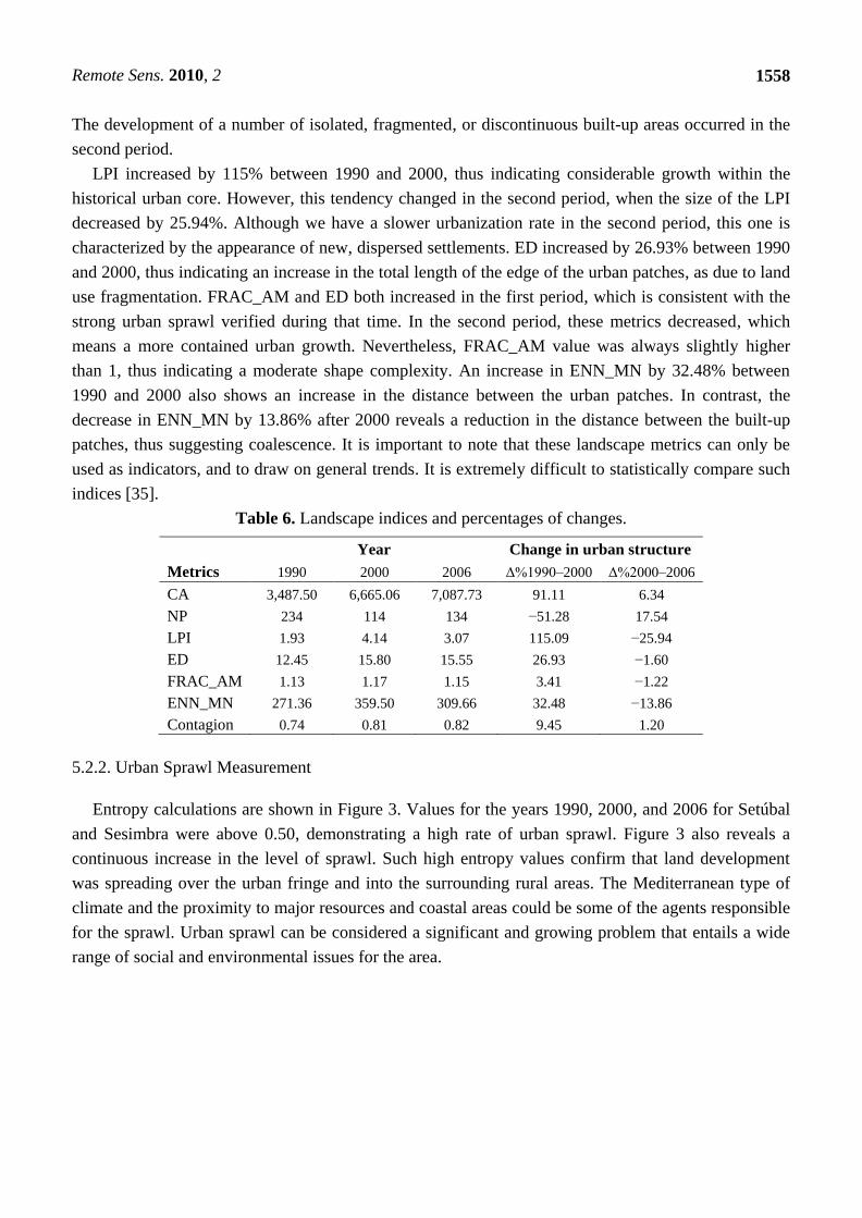
5.2.2. Urban Sprawl Measurement

Entropy calculations are shown in Figure 3. Values for the years 1990, 2000, and 2006 for Setúbal

and Sesimbra were above 0.50, demonstrating a high rate of urban sprawl. Figure 3 also reveals a

continuous increase in the level of sprawl. Such high entropy values confirm that land development

was spreading over the urban fringe and into the surrounding rural areas. The Mediterranean type of

climate and the proximity to major resources and coastal areas could be some of the agents responsible

for the sprawl. Urban sprawl can be considered a significant and growing problem that entails a wide

range of social and environmental issues for the area.


1559

Figure 3. Urban sprawl measurement.

0.73

0.83

0.88

0.73

0.80

0.89

0.70

0.72

0.74

0.76

0.78

0.80

0.82

0.84

0.86

0.88

0.90

1990 2000 2006

Entropy

Year

Setubal

Sesimbra

5.3. Land Cover Modeling and Validation

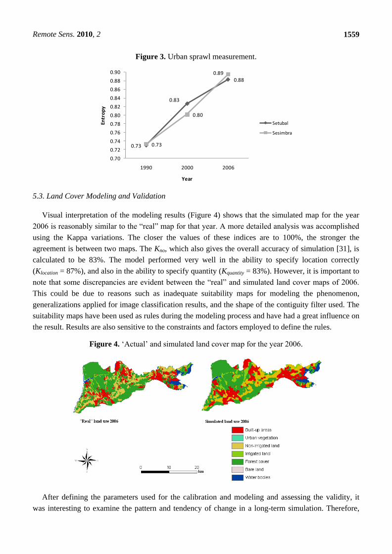
Visual interpretation of the modeling results (Figure 4) shows that the simulated map for the year

2006 is reasonably similar to the ―real‖ map for that year. A more detailed analysis was accomplished

using the Kappa variations. The closer the values of these indices are to 100%, the stronger the

agreement is between two maps. The Kno, which also gives the overall accuracy of simulation [31], is

calculated to be 83%. The model performed very well in the ability to specify location correctly

(Klocation = 87%), and also in the ability to specify quantity (Kquantity = 83%). However, it is important to

note that some discrepancies are evident between the ―real‖ and simulated land cover maps of 2006.

This could be due to reasons such as inadequate suitability maps for modeling the phenomenon,

generalizations applied for image classification results, and the shape of the contiguity filter used. The

suitability maps have been used as rules during the modeling process and have had a great influence on

the result. Results are also sensitive to the constraints and factors employed to define the rules.

Figure 4. ‗Actual‘ and simulated land cover map for the year 2006.

After defining the parameters used for the calibration and modeling and assessing the validity, it

was interesting to examine the pattern and tendency of change in a long-term simulation. Therefore,


1560

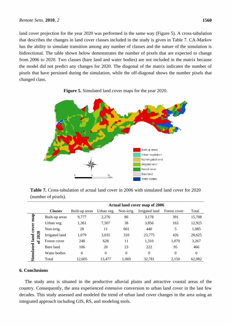
land cover projection for the year 2020 was performed in the same way (Figure 5). A cross-tabulation

that describes the changes in land cover classes included in the study is given in Table 7. CA-Markov

has the ability to simulate transition among any number of classes and the nature of the simulation is

bidirectional. The table shown below demonstrates the number of pixels that are expected to change

from 2006 to 2020. Two classes (bare land and water bodies) are not included in the matrix because

the model did not predict any changes for 2020. The diagonal of the matrix indicates the number of

pixels that have persisted during the simulation, while the off-diagonal shows the number pixels that

changed class.

Figure 5. Simulated land cover maps for the year 2020.

Table 7. Cross-tabulation of actual land cover in 2006 with simulated land cover for 2020

(number of pixels).

Actual land cover map of 2006

Classes Built-up areas Urban veg. Non-irrig. Irrigated land Forest cover Total

Sim

ula

ted

la

nd

co

ver

map

of

20

20

Built-up areas 9,777 2,276 86 3,178 391 15,708

Urban veg. 1,361 7,507 38 3,856 163 12,925

Non-irrig. 28 11 601 440 5 1,085

Irrigated land 1,079 3,035 310 23,775 426 28,625

Forest cover 248 628 11 1,310 1,070 3,267

Bare land 106 20 23 222 95 466

Water bodies 6 0 0 0 0 6

Total 12,605 13,477 1,069 32,781 2,150 62,082

6. Conclusions

The study area is situated in the productive alluvial plains and attractive coastal areas of the

country. Consequently, the area experienced extensive conversion to urban land cover in the last few

decades. This study assessed and modeled the trend of urban land cover changes in the area using an

integrated approach including GIS, RS, and modeling tools.


1561

LULC maps of the study area for the years 2000 and 2006 were obtained using an object-oriented

approach and the derived maps provided new information on spatio-temporal distributions of built-up

areas in the region. Results obtained from classification were validated and employed for further

change analysis and modeling.

A critical analysis of the nature of urban land cover change was addressed and quantified using

landscape metrics and urban sprawl measurements. Each of the metrics provided information on the

nature of each index for the study site. The sprawl measurement, with the Shannon Entropy index,

supports the claim that there has been a high rate of sprawl and dispersion of urban development in the

studied period, causing a significant impact on the urban fringe. The driving forces behind the sprawl

could be many, but one of the major factors was population growth, particularly in the period after

1970, with the end of Portuguese overseas colonies.

The spatial simulation technique employed produced satisfactory results that were confirmed by

various Kappa summaries. This allowed us to project land change until the year 2020. Results indicate

that urban growth might continue to expand further in the future, and might have an undeniable impact

on land resources, unless some preservation mechanism is enacted. Future projections presented a

satisfactory output for short term forecasting. However, it is important to caution that the approach

applied in this study may not be the best approach for long-term simulation. CA-Markov analysis does

not only consider a change from non-built to built-up areas, but also any kind of transition among any

of the feature classes included in the analyses. A change from built-up areas to non-built-up areas is

less likely in rapidly growing urban areas, but the simulation model applied does consider this

possibility. Future work will consider all these limitations and apply an advanced modeling approach

that would allow for long-term simulation.

Acknowledgements

The work has been supported by the European Commission, Erasmus Mundus Programme, M.Sc.

in Geospatial Technologies, project NO. 2007-0064. The authors would like to thank Tarmo K.

Remmel (York University, Canada) and Steve Drury (Open University, UK) for their helpful reviews

of this paper.

References

1. Yuan, F.; Sawaya, K.; Loeffelholz, B.; Bauer, M. Land cover classification and change analysis of

the Twin cities (Minnesota) Metropolitan Area by multitemporal Landsat Remote Sens. Environ..

Remote Sens. Environ. 2005, 98, 317-328.

2. Brockerhoff, M.P. An urbanizing world. Pop. Bull. 2000, 55, 3-44.

3. Civco, D.; Hurd, J.; Wilson, E.; Son, M; Zhang, Y. A comparison of land use and land cover

change detection methods. In Proceedings of American Society for Photogrammetry and Remote

Sensing/American Congress on Surveying and Mapping, Washington, DC, USA, April 2002.

4. Alkheder, S.; Shan, J. Cellular Automata urban growth simulation and evaluation: A case study of

Indianapolis. Geomatics Engineering, School of Civil Engineering, Purdue University, 2005.

Available online: http://www.geocomputation.org/2005/Alkheder.pdf (accessed on May 2, 2008).


1562

5. Hand, C. Simple cellular automata on a spreadsheet. Comput. Higher Educ. Econ. Rev. 2005, 17,

9-13.

6. Cabral, P. Étude de la croissance urbaine par télédétection, sig et modélisation Le cas des

Concelhos de Sintra et Cascais (Portugal). Ph.D. Dissertation; École des Hautes Études en

Sciences Sociales, Paris, France, 2006.

7. Carlos, S. Some points in the management of natural spaces in the Lisbon Metropolitan Area,

2005. Available online: http://www.fedenatur.org/docs/docs/58.pdf (accessed on December 16,

2008).

8. AML. Área Metropolitana de Lisboa, 2005. Available online: www.aml.pt (accessed on October

15, 2008).

9. ESA. Earth Observation—Principal Investigator Portal: European Space Agency 2009. Available

online: http://eopi.esa.int/esa/esa?cmd=aodetail&aoname=IMAGE2006 (accessed on November

25, 2009).

10. Lu, D.; Weng, Q. A survey of image classification methods and techniques for improving

classification performance. Int. J. Remote Sens. 2007, 28, 823-870.

11. Farzaneh, A. Application of image fusion (object fusion) for forest classification in Northern

forests of Iran. J. Agr. Sci. Tech. 2007, 9, 43-54.

12. Araya, Y.; Hergarten, C. A comparison of pixel and object-based land cover classification: A case

study of the Asmara region, Eritrea. In Geo-environment and landscape evolution III Conference,

Southampton, UK, 2008, pp. 233-243.

13. Moeller, M.S.; Stefanov, W.L.; Netband, M. Characterizing land cover changes in a rapidly growing

metropolitan area using long term satellite imagery. In Proceedings of the 2004 Annual Meeting of

the American Society for Photogrammetry and Remote Sensing, Denver, CO, USA, 2004.

14. Im, J.; Jensen, J.; Tullis J. Object-based change detection using correlation image analysis and

image segmentation. Int. J. Remote Sens. 2008, 29, 399-423.

15. Congalton, R.G. A review of assessing the accuracy of classifications of remotely sensed data.

Remote Sens. Environ. 1991, 37, 35-46.

16. Rosenfield, G.; Fitzpatrick-Lins, K. A coefficient agreement as a measure of thematic

classification accuracy. Photogramm. Eng. Remote Sensing 1986, 52, 223-227.

17. Cabral, P.; Geroyannis, H.; Gilg, J.-P.; Painho, M. Analysis and modeling of land-use and

land-cover change in Sintra-Cascais area. In Proceedings of 8th Agile Conference, Estoril,

Portugal, May 2005.

18. Herold, M.; Scepan, J.; Clarke, C. The use of remote sensing and landscape metrics to describe

structures and changes in urban land uses. Environ. Plan. 2002, 34, 1443-1458.

19. McGarigal, K.; Cushman, M.; Neel, C.; Ene, E. FRAGSTATS; Spatial pattern analysis program for

categorical maps. University of Massachusetts: Amherst, MA, USA, 2002. Available online:

www.umass.edu/landeco/research/fragstats/fragstats.html (accessed on October 10, 2008).

20. Alberti, M.; Waddel, P. An integrated urban development and ecological simulation model.

Integrated Assessment. 2000, 1, 215-227.

21. Herold, M.; Goldstein, N.; Clarke, K. The spatio-temporal form of urban growth: Measurement,

analysis and modeling. Remote Sens. Environ. 2003, 85, 95-105.


1563

22. Barnes, B.; Morgan J.; Roberge M.; Lowe, S. Sprawl development: Its patterns, consequences,

and measurement. Center for Geographic Information Services, Towson University, Towson,

MD, USA, 2002. Available online: http://chesapeake.townson.edu/landscape/urbansprawl/

download/Sprawl_white_paper.pdf (accessed on December 16, 2008).

23. Sun, H.; Forsythe, W.; Waters, N. Modeling urban land use change and urban sprawl: Calgary,

Alberta, Canada. Networks Spatial Econ. 2007, 7, 353-376.

24. Lata, M.; Prasad, K.; Bandarinath, K.; Raghavaswamy, R.; Rao, S. Measuring urban sprawl: A

case study of Hyderabad. GIS Development 2001, 5. Available online:

http://www.gisdevelopment.net/application/urban/sprawl/urbans0004.htm (accessed on December

15, 2008).

25. Yeh, A.; Li, X. Measurement and monitoring of urban sprawl in a rapidly growing region using

entropy. Photogramm. Eng. Remote Sensing 2001, 67, 83-90.

26. Sudhira, H.S.; Ramachandra, T.V.; Jagadish, K.S. Urban sprawl: Metrics, dynamics and modeling

using GIS. Int. J. Appl. Earth Obs. Geoinf. 2004, 5, 29-39.

27. Eastman, R. IDRISI 32 Guide to GIS and Image Processing; Clark University, Worcester, MA,

USA, 2000; Volume 1, pp. 109-142.

28. Direcção Geral de Ordenamento do Território e Desenvolvimento Urbano (DGOTDU). Servidões

e Restrições de Utilidade Pública, 2009. Available online: http://www.dgotdu.pt (accessed on

November 25, 2008).

29. Rocha, J.; Ferreira, C.; Simoes, J.; Tenedorio, A. Modeling coastal and land use evolution patterns

through neural network and cellular automata integration. J. Coastal Res. 2007, 50,

827-831.

30. Cabral, P.; Zamyatin, A. Three land change models for urban dynamics analysis in Sintra-Cascais

area. In Proceedings of the 1st EARSel Workshop of the SIG Urban remote sensing,

Humboldt-Universität zu Berlin, Berlin, Germany, March 2006.

31. Pontius, G.R. Quantification error versus location error in comparison of categorical maps.

Photogramm. Eng. Remote Sensing 2000, 66, 1011-1016.

32. Dushku, A.; Brown, S. Spatial modeling of baselines for LULUCF Carbon projects: The

GEOMOD modeling approach. In International Conference on Tropical Forests and Climate

Change, Manila, Philippines, October 2003.

33. Anderson, J.; Hardy, E.; Roach, J.; Witner, R. A Land Use and Land Cover Classification System

for Use with Remote Sensor Data; US Geological Survey Professional Paper 964, USGS:

Washington, DC, USA, 1976.

34. Muzein, B.S. Remote sensing and GIS for land cover/land use change detection and analysis in

the semi-natural ecosystems and agriculture landscapes of the central Ethiopian Rift Valley. Ph.D.

Dissertation, Techniche Universität Dresden, Dresden, Germany, 2006.

35. Remmel, T.K.; Csillag, F. When are two landscape pattern indices significantly different? J.

Geogr. Syst. 2003, 5, 331-351.

© 2010 by the authors; licensee MDPI, Basel, Switzerland. This article is an Open Access article

distributed under the terms and conditions of the Creative Commons Attribution license

(http://creativecommons.org/licenses/by/3.0/).

analysis and modeling of urban land cover change in ... · analysis and modeling of urban land...

Documents