an overview of depth cameras and range scanners based on

HAL Id: hal-01325045https://hal.inria.fr/hal-01325045

Submitted on 1 Jun 2016

HAL is a multi-disciplinary open accessarchive for the deposit and dissemination of sci-entific research documents, whether they are pub-lished or not. The documents may come fromteaching and research institutions in France orabroad, or from public or private research centers.

L’archive ouverte pluridisciplinaire HAL, estdestinée au dépôt et à la diffusion de documentsscientifiques de niveau recherche, publiés ou non,émanant des établissements d’enseignement et derecherche français ou étrangers, des laboratoirespublics ou privés.

An Overview of Depth Cameras and Range ScannersBased on Time-of-Flight Technologies

Radu Horaud, Miles Hansard, Georgios Evangelidis, Clément Ménier

To cite this version:Radu Horaud, Miles Hansard, Georgios Evangelidis, Clément Ménier. An Overview of Depth Camerasand Range Scanners Based on Time-of-Flight Technologies. Machine Vision and Applications, SpringerVerlag, 2016, 27 (7), pp.1005-1020. �10.1007/s00138-016-0784-4�. �hal-01325045�

https://hal.inria.fr/hal-01325045

https://hal.archives-ouvertes.fr

Machine Vision and Applications

An Overview of Depth Cameras and Range Scanners Based onTime-of-Flight Technologies

Radu Horaud · Miles Hansard · Georgios Evangelidis · Clement Menier

Received: November 2015 / Accepted: May 2016

Abstract Time-of-flight (TOF) cameras are sensors

that can measure the depths of scene-points, by illumi-

nating the scene with a controlled laser or LED source,

and then analyzing the reflected light. In this paper

we will first describe the underlying measurement prin-

ciples of time-of-flight cameras, including: (i) pulsed-

light cameras, which measure directly the time taken

for a light pulse to travel from the device to the object

and back again, and (ii) continuous-wave modulated-

light cameras, which measure the phase difference be-

tween the emitted and received signals, and hence ob-

tain the travel time indirectly. We review the main

existing designs, including prototypes as well as com-

mercially available devices. We also review the relevant

camera calibration principles, and how they are applied

to TOF devices. Finally, we discuss the benefits andchallenges of combined TOF and color camera systems.

This work has received funding from the French Agence Na-tionale de la Recherche (ANR) under the MIXCAM projectANR-13-BS02-0010-01, and from the European ResearchCouncil (ERC) under the Advanced Grant VHIA project340113.

R. Horaud and G. EvangelidisINRIA Grenoble Rhone-AlpesMontbonnot Saint-Martin, FranceE-mail: [email protected], [email protected]

M. HansardSchool of Electronic Engineering and Computer ScienceQueen Mary University of London, United KingdomE-mail: [email protected]

C. Menier4D View SolutionsGrenoble, FranceE-mail: [email protected]

Keywords LIDAR · range scanners · single photon

avalanche diode · time-of-flight cameras · 3D computer

vision · active-light sensors

1 Introduction

During the last decades, there has been a strong in-

terest in the design and development of range-sensing

systems and devices. The ability to remotely measure

range is extremely useful and has been extensively used

for mapping and surveying, on board of ground vehicles,

aircraft, spacecraft and satellites, and for civil as well

as military purposes. NASA has identified range sens-

ing as a key technology for enabling autonomous and

precise planet landing with both robotic and crewed

space missions, e.g., [Amzajerdian et al., 2011]. More re-

cently, range sensors of various kinds have been used in

computer graphics and computer vision for 3-D object

modeling [Blais, 2004], Other applications include ter-

rain measurement, simultaneous localization and map-

ping (SLAM), autonomous and semi-autonomous vehi-

cle guidance (including obstacle detection), as well as

object grasping and manipulation. Moreover, in com-

puter vision, range sensors are ubiquitous in a num-

ber of applications, including object recognition, human

motion capture, human-computer interaction, and 3-D

reconstruction [Grzegorzek et al., 2013].

There are several physical principles and associated

technologies that enable the fabrication of range sen-

sors. One type of range sensor is known as LIDAR,

which stands either for “Light Imaging Detection And

Ranging” or for “LIght and raDAR”. LIDAR is a remote-

sensing technology that estimates range (or distance,

or depth) by illuminating an object with a collimated

2 R. Horaud, M. Hansard, G. Evangelidis & C. Menier

laser beam, followed by detecting the reflected light us-

ing a photodetector. This remote measurement prin-

ciple is also known as time of flight (TOF). Because

LIDARs use a fine laser-beam, they can estimate dis-

tance with high resolution. LIDARs can use ultraviolet,

visible or infrared light. They can target a wide range of

materials, including metallic and non-metallic objects,

rocks, vegetation, rain, clouds, and so on – but exclud-

ing highly specular materials.

The vast majority of range-sensing applications re-

quire an array of depth measurements, not just a sin-

gle depth value. Therefore, LIDAR technology must be

combined with some form of scanning, such as a rotat-

ing mirror, in order to obtain a row of horizontally adja-

cent depth values. Vertical depth values can be obtained

by using two single-axis rotating mirrors, by employing

several laser beams with their dedicated light detectors,

or by using mirrors at fixed orientations. In all cases,

both the vertical field of view and the vertical resolu-

tion are inherently limited. Alternatively, it is possible

to design a scannerless device: the light coming from a

single emitter is diverged such that the entire scene of

interest is illuminated, and the reflected light is imaged

onto a two-dimensional array of photodetectors, namely

a TOF depth camera. Rather than measuring the in-

tensity of the ambient light, as with standard cameras,

TOFcameras measure the reflected light coming from

the camera’s own light-source emitter.

Therefore, both TOF range scanners and cameras

belong to a more general category of LIDARs that com-

bine a single or multiple laser beams, possibly mounted

onto a rotating mechanism, with a 2D array of light de-

tectors and time-to-digital converters, to produce 1-D

or 2-D arrays of depth values. Broadly speaking, there

are two ways of measuring the time of flight [Remondino

and Stoppa, 2013], and hence two types of sensors:

– Pulsed-light sensors directly measure the round-trip

time of a light pulse. The width of the light pulse

is of a few nanoseconds. Because the pulse irradi-

ance power is much higher than the background

(ambient) irradiance power, this type of TOF cam-

era can perform outdoors, under adverse conditions,

and can take long-distance measurements (from a

few meters up to several kilometers). Light-pulse de-

tectors are based on single photon avalanche diodes

(SPAD) for their ability to capture individual pho-

tons with high time-of-arrival resolution [Cova et al.,

1981], approximatively 10 picoseconds (10−11 s).

– Continuous-wave (CW) modulation sensors measure

the phase differences between an emitted continuous

sinusoidal light-wave signal and the backscattered

signals received by each photodetector [Lange and

Seitz, 2001]. The phase difference between emitted

and received signals is estimated via cross-correlation

(demodulation). The phase is directly related to dis-

tance, given the known modulation frequency. These

sensors usually operate indoors, and are capable of

short-distance measurements only (from a few cen-

timeters to several meters). One major shortcoming

of this type of depth camera is the phase-wrapping

ambiguity [Hansard et al., 2013].

This paper overviews pulsed-light (section 2) and

continuous wave (section 4) range technologies, their

underlying physical principles, design, scanning mecha-

nisms, advantages, and limitations. We review the prin-

cipal technical characteristics of some of the commer-

cially available TOF scanners and cameras as well as of

some laboratory prototypes. Then we discuss the geo-

metric and optical models together with the associated

camera calibration techniques that allow to map raw

TOF measurements onto Cartesian coordinates and hence

to build 3D images or point clouds (section 6). We also

address the problem of how to combine TOF and color

cameras for depth-color fusion and depth-stereo fusion

(section 7).

2 Pulsed-Light Technology

As already mentioned, pulsed-light depth sensors are

composed of both a light emitter and light receivers.

The sensor sends out pulses of light emitted by a laser

or by a laser-diode (LD). Once reflected onto an object,

the light pulses are detected by an array of photodi-

odes that are combined with time-to-digital converters

(TDCs) or with time-to-amplitude circuitry. There are

two possible setups which will be referred to as range

scanner and 3D flash LIDAR camera:

– A TOF range scanner is composed of a single laser

that fires onto a single-axis rotating mirror. This en-

ables a very wide field of view in one direction (up to

360◦) and a very narrow field of view in the other di-

rection. One example of such a range scanner is the

Velodyne family of sensors [Schwarz, 2010] that fea-

ture a rotating head equipped with several (16, 32 or

64) LDs, each LD having its own dedicated photode-

tector, and each laser-detector pair being precisely

aligned at a predetermined vertical angle, thus giv-

ing a wide vertical field of view. Another example of

this type of TOF scanning device was recently de-

veloped by the Toyota Central R&D Laboratories:

the sensor is based on a single laser combined with a

An Overview of Depth Cameras and Range Scanners Based on Time-of-Flight Technologies 3

multi-facet polygonal (rotating) mirror. Each polyg-

onal facet has a slightly different tilt angle, as a re-

sult each facet of the mirror reflects the laser beam

into a different vertical direction, thus enhancing the

vertical field-of-view resolution [Niclass et al., 2013].

– A 3D flash LIDAR camera uses the light beam from

a single laser that is spread using an optical dif-

fuser, in order to illuminate the entire scene of in-

terest. A 1-D or 2-D array of photo-detectors is then

used to obtain a depth image. A number of sen-

sor prototypes were developed using single photon

avalanche diodes (SPADs) integrated with conven-

tional CMOS timing circuitry, e.g., a 1-D array of

64 elements [Niclass et al., 2005], 32×32 arrays [Al-

bota et al., 2002, Stoppa et al., 2007], or a 128×128

array [Niclass et al., 2008]. A 3-D Flash LIDAR cam-

era, featuring a 128×128 array of SPADs, described

in [Amzajerdian et al., 2011], is commercially avail-

able.

2.1 Avalanche Photodiodes

One of the basic elements of any TOF camera is an

array of photodetectors, each detector has its own tim-

ing circuit to measure the range to the corresponding

point in the scene. Once a light pulse is emitted by a

laser and reflected onto an object, only a fraction of the

optical energy is received by the detector – the energy

fall-off is inversely proportional to the square of the dis-

tance. When an optical diffuser is present, this energy

is further divided among multiple detectors. If a depth

precision of a few centimeters is needed, the timing pre-

cision must be less than a nanosecond.1 Moreover, the

bandwidth of the detection circuit must be high, which

also means that the noise is high, thus competing with

the weak signal.

The vast majority of pulse-light receivers are based

on arrays of single photon avalanche diodes which are

also referred to as Geiger-mode avalanche photodiodes

(G-APD). A SPAD is a special way of operating an

avalanche photodiode (APD), namely it produces a fast

electrical pulse of several volts amplitude in response to

the detection of a single photon. This electrical pulse

then generally trigers a digital CMOS circuit integrated

into each pixel. An integrated SPAD-CMOS array is a

compact, low-power and all-solid-state sensor [Niclass

et al., 2008].

The elementary building block of semiconductor diodes

and hence of photodiodes is the p−n junction, namely

1 As the light travels at 3 × 1010 cm/s, 1 ns (or 10−9 s)corresponds to 30cm.

the boundary between two types of semiconductor ma-

terials, p-type and n-type. This is created by doping

which is a process that consists of adding impurities

into an extremely pure semiconductor for the purpose of

modifying its electrical (conductivity) properties. Ma-

terials conduct electricity if they contain mobile charge

carriers. There are two types of charge carriers in a

semiconductor: free electrons and electron holes. When

an electric field exists in the vicinity of the junction, it

keeps free electrons confined on the n-side and electron

holes confined on the p-side.

There are two types of p−n diodes: forward-bias and

reverse-bias. In forward-bias, the p-side is connected

with the positive terminal of an electric power supply

and the n-side is connected with the negative terminal.

Both electrons and holes are pushed towards the junc-

tion. In reverse-bias, the p-side is connected with the

negative terminal and the n-side is connected with the

positive terminal. Otherwise said, the voltage on the

n-side is higher than the voltage on the p-side. In this

case both electrons and holes are pushed away from the

junction.

A photodiode is a semiconductor diode that con-

verts light into current. The current is generated when

photons are absorbed in the photodiode. Photodiodes

are similar to regular semiconductor diodes. A photo-

diode is designed to operate in reverse bias. An APD

is a variation of a p− n junction photodiode. When an

incident photon of sufficient energy is absorbed in the

region where the field exists, an electron-hole pair is

generated. Under the influence of the field, the electron

drifts to the n-side and the hole drifts to the p-side,

resulting in the flow of photocurrent (i.e., the current

induced by the detection of photons) in the external

circuit. When a photodiode is used to detect light, the

number of electron-hole pairs generated per incident

photon is at best unity.

An APD detects light by using the same principle

[Aull et al., 2002]. The difference between an APD and

an ordinary p− n junction photodiode is that an APD

is designed to support high electric fields. When an

electron-hole pair is generated by photon absorption,

the electron (or the hole) can accelerate and gain suf-

ficient energy from the field to collide with the crystal

lattice and generate another electron-hole pair, losing

some of its kinetic energy in the process. This process is

known as impact ionization. The electron can accelerate

again, as can the secondary electron or hole, and create

more electron-hole pairs, hence the term “avalanche”.

After a few transit times, a competition develops

between the rate at which electron-hole pairs are being

generated by impact ionization (analogous to a birth


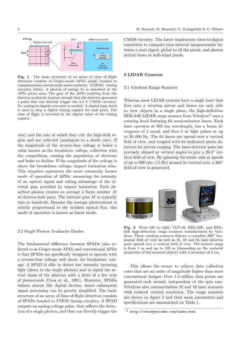
Fig. 1 The basic structure of an array of time of flightdetectors consists of Geiger-mode APDs (pink) bonded tocomplementary-metal-oxide-semiconductor (CMOS) timingcircuitry (blue). A photon of energy hv is absorbed in theAPD active area. The gain of the APD resulting from theelectron avalanche is great enough that the detector generatesa pulse that can directly trigger the 3.3 V CMOS circuitry.No analog-to-digital converter is needed. A digital logic latchis used to stop a digital timing register for each pixel. Thetime of flight is recorded in the digital value of the timingregister.

rate) and the rate at which they exit the high-field re-

gion and are collected (analogous to a death rate). If

the magnitude of the reverse-bias voltage is below a

value known as the breakdown voltage, collection wins

the competition, causing the population of electrons

and holes to decline. If the magnitude of the voltage is

above the breakdown voltage, impact ionization wins.

This situation represents the most commonly known

mode of operation of APDs: measuring the intensity

of an optical signal and taking advantage of the in-

ternal gain provided by impact ionization. Each ab-

sorbed photon creates on average a finite number M

of electron-hole pairs. The internal gain M is typically

tens or hundreds. Because the average photocurrent is

strictly proportional to the incident optical flux, this

mode of operation is known as linear mode.

2.2 Single Photon Avalanche Diodes

The fundamental difference between SPADs (also re-

ferred to as Geiger-mode APD) and conventional APDs

is that SPADs are specifically designed to operate with

a reverse-bias voltage well above the breakdown volt-

age. A SPAD is able to detect low intensity incoming

light (down to the single photon) and to signal the ar-

rival times of the photons with a jitter of a few tens

of picoseconds [Cova et al., 1981]. Moreover, SPADs

behave almost like digital devices, hence subsequent

signal processing can be greatly simplified. The basic

structure of an array of time-of-flight detectors consists

of SPADs bonded to CMOS timing circuitry. A SPAD

outputs an analog voltage pulse, that reflects the detec-

tion of a single photon, and that can directly trigger the

CMOS circuitry. The latter implements time-to-digital

converters to compute time-interval measurements be-

tween a start signal, global to all the pixels, and photon

arrival times in individual pixels.

3 LIDAR Cameras

3.1 Velodyne Range Scanners

Whereas most LIDAR systems have a single laser that

fires onto a rotating mirror and hence are only able

to view objects in a single plane, the high-definition

HDL-64E LIDAR range scanner from Velodyne2 uses a

rotating head featuring 64 semiconductor lasers. Each

laser operates at 905 nm wavelength, has a beam di-

vergence of 2 mrad, and fires 5 ns light pulses at up

to 20, 000 Hz. The 64 lasers are spread over a vertical

field of view, and coupled with 64 dedicated photo de-

tectors for precise ranging. The laser-detector pairs are

precisely aligned at vertical angles to give a 26.8◦ ver-

tical field of view. By spinning the entire unit at speeds

of up to 900 rpm (15 Hz) around its vertical axis, a 360◦

field-of-view is generated.

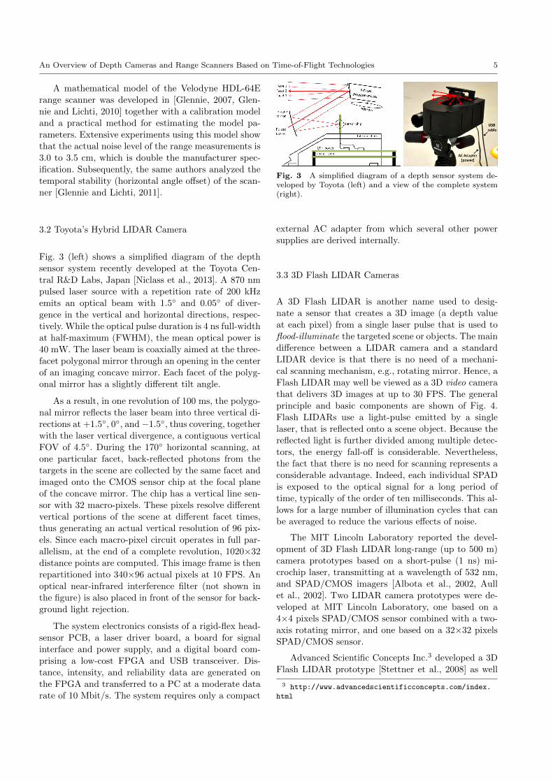
Fig. 2 From left to right: VLP-16, HDL-32E, and HDL-64E high-definition range scanners manufactured by Velo-dyne. These rotating scanners feature a complete 360◦ hor-izontal field of view as well as 16, 32 and 64 laser-detectorpairs spread over a vertical field of view. The sensors rangeis from 1 m and up to 120 m (depending on the materialproperties of the scanned object) with a accuracy of 2 cm.

This allows the sensor to achieve data collection

rates that are an order of magnitude higher than most

conventional designs. Over 1.3 million data points are

generated each second, independent of the spin rate.

Velodyne also commercializes 32 and 16 laser scanners

with reduced vertical resolution. The range scanners

are shown on figure 2 and their main parameters and

specifications are summarized on Table 1.

2 http://velodynelidar.com/index.html


A mathematical model of the Velodyne HDL-64E

range scanner was developed in [Glennie, 2007, Glen-

nie and Lichti, 2010] together with a calibration model

and a practical method for estimating the model pa-

rameters. Extensive experiments using this model show

that the actual noise level of the range measurements is

3.0 to 3.5 cm, which is double the manufacturer spec-

ification. Subsequently, the same authors analyzed the

temporal stability (horizontal angle offset) of the scan-

ner [Glennie and Lichti, 2011].

3.2 Toyota’s Hybrid LIDAR Camera

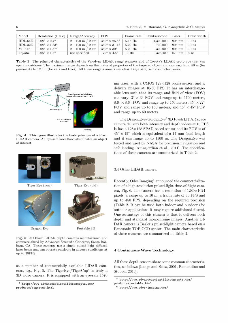
Fig. 3 (left) shows a simplified diagram of the depth

sensor system recently developed at the Toyota Cen-

tral R&D Labs, Japan [Niclass et al., 2013]. A 870 nm

pulsed laser source with a repetition rate of 200 kHz

emits an optical beam with 1.5◦ and 0.05◦ of diver-

gence in the vertical and horizontal directions, respec-

tively. While the optical pulse duration is 4 ns full-width

at half-maximum (FWHM), the mean optical power is

40 mW. The laser beam is coaxially aimed at the three-

facet polygonal mirror through an opening in the center

of an imaging concave mirror. Each facet of the polyg-

onal mirror has a slightly different tilt angle.

As a result, in one revolution of 100 ms, the polygo-

nal mirror reflects the laser beam into three vertical di-

rections at +1.5◦, 0◦, and−1.5◦, thus covering, together

with the laser vertical divergence, a contiguous vertical

FOV of 4.5◦. During the 170◦ horizontal scanning, at

one particular facet, back-reflected photons from the

targets in the scene are collected by the same facet and

imaged onto the CMOS sensor chip at the focal plane

of the concave mirror. The chip has a vertical line sen-

sor with 32 macro-pixels. These pixels resolve different

vertical portions of the scene at different facet times,

thus generating an actual vertical resolution of 96 pix-

els. Since each macro-pixel circuit operates in full par-

allelism, at the end of a complete revolution, 1020×32

distance points are computed. This image frame is then

repartitioned into 340×96 actual pixels at 10 FPS. An

optical near-infrared interference filter (not shown in

the figure) is also placed in front of the sensor for back-

ground light rejection.

The system electronics consists of a rigid-flex head-

sensor PCB, a laser driver board, a board for signal

interface and power supply, and a digital board com-

prising a low-cost FPGA and USB transceiver. Dis-

tance, intensity, and reliability data are generated on

the FPGA and transferred to a PC at a moderate data

rate of 10 Mbit/s. The system requires only a compact

Fig. 3 A simplified diagram of a depth sensor system de-veloped by Toyota (left) and a view of the complete system(right).

external AC adapter from which several other power

supplies are derived internally.

3.3 3D Flash LIDAR Cameras

A 3D Flash LIDAR is another name used to desig-

nate a sensor that creates a 3D image (a depth value

at each pixel) from a single laser pulse that is used to

flood-illuminate the targeted scene or objects. The main

difference between a LIDAR camera and a standard

LIDAR device is that there is no need of a mechani-

cal scanning mechanism, e.g., rotating mirror. Hence, a

Flash LIDAR may well be viewed as a 3D video camera

that delivers 3D images at up to 30 FPS. The general

principle and basic components are shown of Fig. 4.

Flash LIDARs use a light-pulse emitted by a single

laser, that is reflected onto a scene object. Because the

reflected light is further divided among multiple detec-

tors, the energy fall-off is considerable. Nevertheless,

the fact that there is no need for scanning represents a

considerable advantage. Indeed, each individual SPAD

is exposed to the optical signal for a long period of

time, typically of the order of ten milliseconds. This al-

lows for a large number of illumination cycles that can

be averaged to reduce the various effects of noise.

The MIT Lincoln Laboratory reported the devel-

opment of 3D Flash LIDAR long-range (up to 500 m)

camera prototypes based on a short-pulse (1 ns) mi-

crochip laser, transmitting at a wavelength of 532 nm,

and SPAD/CMOS imagers [Albota et al., 2002, Aull

et al., 2002]. Two LIDAR camera prototypes were de-

veloped at MIT Lincoln Laboratory, one based on a

4×4 pixels SPAD/CMOS sensor combined with a two-

axis rotating mirror, and one based on a 32×32 pixels

SPAD/CMOS sensor.

Advanced Scientific Concepts Inc.3 developed a 3D

Flash LIDAR prototype [Stettner et al., 2008] as well

3 http://www.advancedscientificconcepts.com/index.

html


Model Resolution (H×V) Range/Accuracy FOV Frame rate Points/second Laser Pulse width

HDL-64E 0.08◦ × 0.4◦ 2 – 120 m / 2 cm 360◦ × 26.8◦ 5-15 Hz 1,300,000 905 nm 10 nsHDL-32E 0.08◦ × 1.33◦ 2 – 120 m / 2 cm 360◦ × 31.4◦ 5-20 Hz 700,000 905 nm 10 nsVLP-16 0.08◦ × 1.87◦ 2 – 100 m / 2 cm 360◦ × 30◦ 5-20 Hz 300,000 905 nm 10 nsToyota 0.05◦ × 1.5◦ not specified 170◦ × 4.5◦ 10 Hz 326,400 870 nm 4 ns

Table 1 The principal characteristics of the Velodyne LIDAR range scanners and of Toyota’s LIDAR prototype that canoperate outdoors. The maximum range depends on the material properties of the targeted object and can vary from 50 m (forpavement) to 120 m (for cars and trees). All these range scanners use class 1 (eye safe) semiconductor lasers.

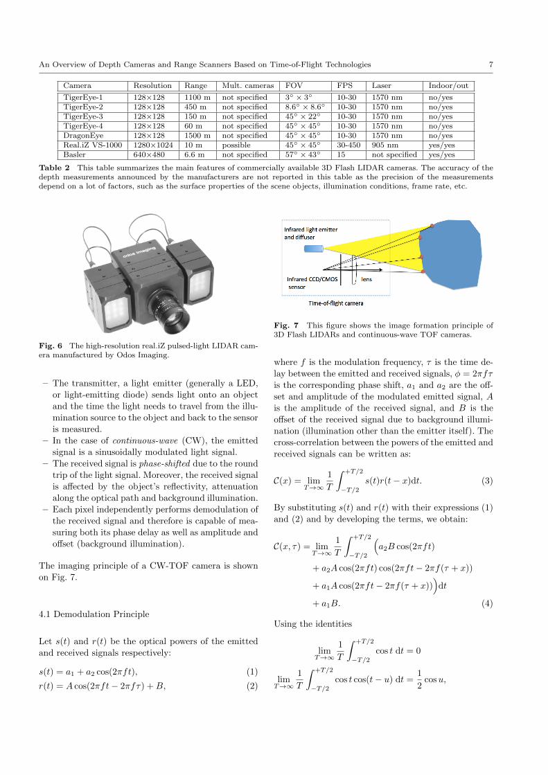
Fig. 4 This figure illustrates the basic principle of a FlashLIDAR camera. An eye-safe laser flood-illuminates an objectof interest.

Tiger Eye (new) Tiger Eye (old)

Dragon Eye Portable 3D

Fig. 5 3D Flash LIDAR depth cameras manufactured andcommercialized by Advanced Scientific Concepts, Santa Bar-bara, CA. These cameras use a single pulsed-light diffusedlaser beam and can operate outdoors in adverse conditions atup to 30FPS.

as a number of commercially available LIDAR cam-

eras, e.g., Fig. 5. The TigerEye/TigerCup4 is truly a

3D video camera. It is equipped with an eye-safe 1570

4 http://www.advancedscientificconcepts.com/

products/tigercub.html

nm laser, with a CMOS 128×128 pixels sensor, and it

delivers images at 10-30 FPS. It has an interchange-

able lens such that its range and field of view (FOV)

can vary: 3◦ × 3◦ FOV and range up to 1100 meters,

8.6◦× 8.6◦ FOV and range up to 450 meters, 45◦× 22◦

FOV and range up to 150 meters, and 45◦ × 45◦ FOV

and range up to 60 meters.

The DragonEye/GoldenEye5 3D Flash LIDAR space

camera delivers both intensity and depth videos at 10 FPS.

It has a 128×128 SPAD based sensor and its FOV is of

45◦ × 45◦ which is equivalent of a 17 mm focal length

and it can range up to 1500 m. The DragonEye was

tested and used by NASA for precision navigation and

safe landing [Amzajerdian et al., 2011]. The specifica-

tions of these cameras are summarized in Table 2.

3.4 Other LIDAR camera

Recently, Odos Imaging6 announced the commercializa-

tion of a high-resolution pulsed-light time-of-flight cam-

era, Fig. 6. The camera has a resolution of 1280×1024pixels, a range up to 10 m, a frame rate of 30 FPS and

up to 450 FPS, depending on the required precision

(Table 2. It can be used both indoor and outdoor (for

outdoor applications it may require additional filters).

One advantage of this camera is that it delivers both

depth and standard monochrome images. Another LI-

DAR camera is Basler’s pulsed-light camera based on a

Panasonic TOF CCD sensor. The main characteristics

of these cameras are summarized in Table 2.

4 Continuous-Wave Technology

All these depth sensors share some common characteris-

tics, as follows [Lange and Seitz, 2001, Remondino and

Stoppa, 2013]:

5 http://www.advancedscientificconcepts.com/

products/portable.html6 http://www.odos-imaging.com/


Camera Resolution Range Mult. cameras FOV FPS Laser Indoor/out

TigerEye-1 128×128 1100 m not specified 3◦ × 3◦ 10-30 1570 nm no/yesTigerEye-2 128×128 450 m not specified 8.6◦ × 8.6◦ 10-30 1570 nm no/yesTigerEye-3 128×128 150 m not specified 45◦ × 22◦ 10-30 1570 nm no/yesTigerEye-4 128×128 60 m not specified 45◦ × 45◦ 10-30 1570 nm no/yesDragonEye 128×128 1500 m not specified 45◦ × 45◦ 10-30 1570 nm no/yesReal.iZ VS-1000 1280×1024 10 m possible 45◦ × 45◦ 30-450 905 nm yes/yesBasler 640×480 6.6 m not specified 57◦ × 43◦ 15 not specified yes/yes

Table 2 This table summarizes the main features of commercially available 3D Flash LIDAR cameras. The accuracy of thedepth measurements announced by the manufacturers are not reported in this table as the precision of the measurementsdepend on a lot of factors, such as the surface properties of the scene objects, illumination conditions, frame rate, etc.

Fig. 6 The high-resolution real.iZ pulsed-light LIDAR cam-era manufactured by Odos Imaging.

– The transmitter, a light emitter (generally a LED,

or light-emitting diode) sends light onto an object

and the time the light needs to travel from the illu-

mination source to the object and back to the sensor

is measured.

– In the case of continuous-wave (CW), the emitted

signal is a sinusoidally modulated light signal.

– The received signal is phase-shifted due to the round

trip of the light signal. Moreover, the received signal

is affected by the object’s reflectivity, attenuation

along the optical path and background illumination.

– Each pixel independently performs demodulation of

the received signal and therefore is capable of mea-

suring both its phase delay as well as amplitude and

offset (background illumination).

The imaging principle of a CW-TOF camera is shown

on Fig. 7.

4.1 Demodulation Principle

Let s(t) and r(t) be the optical powers of the emitted

and received signals respectively:

s(t) = a1 + a2 cos(2πft), (1)

r(t) = A cos(2πft− 2πfτ) +B, (2)

Fig. 7 This figure shows the image formation principle of3D Flash LIDARs and continuous-wave TOF cameras.

where f is the modulation frequency, τ is the time de-

lay between the emitted and received signals, φ = 2πfτ

is the corresponding phase shift, a1 and a2 are the off-

set and amplitude of the modulated emitted signal, A

is the amplitude of the received signal, and B is the

offset of the received signal due to background illumi-

nation (illumination other than the emitter itself). The

cross-correlation between the powers of the emitted and

received signals can be written as:

C(x) = limT→∞

1

T

∫ +T/2

−T/2s(t)r(t− x)dt. (3)

By substituting s(t) and r(t) with their expressions (1)

and (2) and by developing the terms, we obtain:

C(x, τ) = limT→∞

1

T

∫ +T/2

−T/2

(a2B cos(2πft)

+ a2A cos(2πft) cos(2πft− 2πf(τ + x))

+ a1A cos(2πft− 2πf(τ + x)))

dt

+ a1B. (4)

Using the identities

limT→∞

1

T

∫ +T/2

−T/2cos t dt = 0

limT→∞

1

T

∫ +T/2

−T/2cos t cos(t− u) dt =

1

2cosu,


we obtain:

C(x, τ) =a2A

2cos(2πf(x+ τ)) + a1B. (5)

Using the notations ψ = 2πfx and φ = 2πfτ , we can

write:

C(ψ, φ) =a2A

2cos(ψ + φ) + a1B. (6)

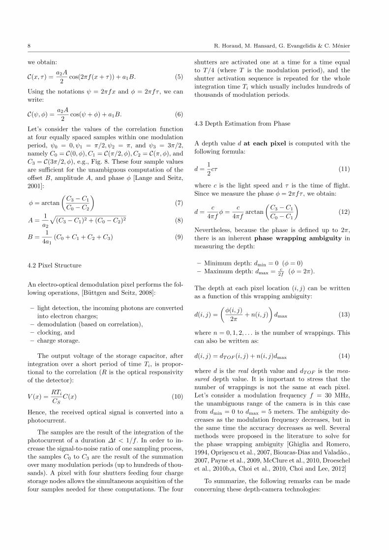
Let’s consider the values of the correlation function

at four equally spaced samples within one modulation

period, ψ0 = 0, ψ1 = π/2, ψ2 = π, and ψ3 = 3π/2,

namely C0 = C(0, φ), C1 = C(π/2, φ), C2 = C(π, φ), and

C3 = C(3π/2, φ), e.g., Fig. 8. These four sample values

are sufficient for the unambiguous computation of the

offset B, amplitude A, and phase φ [Lange and Seitz,

2001]:

φ = arctan

(C3 − C1

C0 − C2

)(7)

A =1

a2

√(C3 − C1)2 + (C0 − C2)2 (8)

B =1

4a1(C0 + C1 + C2 + C3) (9)

4.2 Pixel Structure

An electro-optical demodulation pixel performs the fol-

lowing operations, [Buttgen and Seitz, 2008]:

– light detection, the incoming photons are converted

into electron charges;

– demodulation (based on correlation),

– clocking, and

– charge storage.

The output voltage of the storage capacitor, after

integration over a short period of time Ti, is propor-

tional to the correlation (R is the optical responsivity

of the detector):

V (x) =RTiCS

C(x) (10)

Hence, the received optical signal is converted into a

photocurrent.

The samples are the result of the integration of the

photocurrent of a duration ∆t < 1/f . In order to in-

crease the signal-to-noise ratio of one sampling process,

the samples C0 to C3 are the result of the summation

over many modulation periods (up to hundreds of thou-

sands). A pixel with four shutters feeding four charge

storage nodes allows the simultaneous acquisition of the

four samples needed for these computations. The four

shutters are activated one at a time for a time equal

to T/4 (where T is the modulation period), and the

shutter activation sequence is repeated for the whole

integration time Ti which usually includes hundreds of

thousands of modulation periods.

4.3 Depth Estimation from Phase

A depth value d at each pixel is computed with the

following formula:

d =1

2cτ (11)

where c is the light speed and τ is the time of flight.

Since we measure the phase φ = 2πfτ , we obtain:

d =c

4πfφ =

c

4πfarctan

(C3 − C1

C0 − C1

)(12)

Nevertheless, because the phase is defined up to 2π,

there is an inherent phase wrapping ambiguity in

measuring the depth:

– Minimum depth: dmin = 0 (φ = 0)

– Maximum depth: dmax = c2f (φ = 2π).

The depth at each pixel location (i, j) can be written

as a function of this wrapping ambiguity:

d(i, j) =

(φ(i, j)

2π+ n(i, j)

)dmax (13)

where n = 0, 1, 2, . . . is the number of wrappings. This

can also be written as:

d(i, j) = dTOF (i, j) + n(i, j)dmax (14)

where d is the real depth value and dTOF is the mea-

sured depth value. It is important to stress that the

number of wrappings is not the same at each pixel.

Let’s consider a modulation frequency f = 30 MHz,

the unambiguous range of the camera is in this case

from dmin = 0 to dmax = 5 meters. The ambiguity de-

creases as the modulation frequency decreases, but in

the same time the accuracy decreases as well. Several

methods were proposed in the literature to solve for

the phase wrapping ambiguity [Ghiglia and Romero,

1994, Oprisescu et al., 2007, Bioucas-Dias and Valadao.,

2007, Payne et al., 2009, McClure et al., 2010, Droeschel

et al., 2010b,a, Choi et al., 2010, Choi and Lee, 2012]

To summarize, the following remarks can be made

concerning these depth-camera technologies:


Fig. 8 This figure shows the general principle of the four-bucket method that estimates the demodulated optical signal at fourequally-spaced samples in one modulation period. A CCD/CMOS circuit achieves light detection, demodulation, and chargestorage. The demodulated signal is stored at four equally spaced samples in one modulation period. From these four values, itis then possible to estimate the phase and amplitude of the received signal as well as the amount of background light (offset).

– A CW-TOF camera works at a very precise modula-

tion frequency. Consequently, it is possible to simul-

taneously and synchronously use several CW-TOF

cameras, either by using a different modulation fre-

quency for each one of the cameras, e.g., six cameras

in the case of the SR4000 (Swiss Ranger), or by en-

coding the modulation frequency, e.g., an arbitrary

number of SR4500 cameras.

– In order to increase the signal-to-noise ratio, and

hence the depth accuracy, CW-TOF cameras need

a relatively long integration time (IT), over several

time periods. In turn, this introduces motion blur

[Hansard et al., 2013] (chapter 1) in the presence

of moving objects. Because of the need of long IT,

fast shutter speeds (as done with standard cameras)

cannot be envisaged.

To summarize, the sources of errors of these cameras

are: demodulation, integration, temperature, motion blur,

distance to the target, background illumination, phase

wrapping ambiguity, light scattering, and multiple path

effects. A quantitative analysis of these sources of er-

rors is available in [Foix et al., 2011]. In the case of

several cameras operating simultaneously, interferences

between the different units is an important issue.

5 TOF Cameras

In this section we review the characteristics of some of

the commercially available cameras. We selected those

camera models for which technical and scientific docu-

mentation is readily available. The main specifications

of the overviewed camera models are summarized in

Table 3.

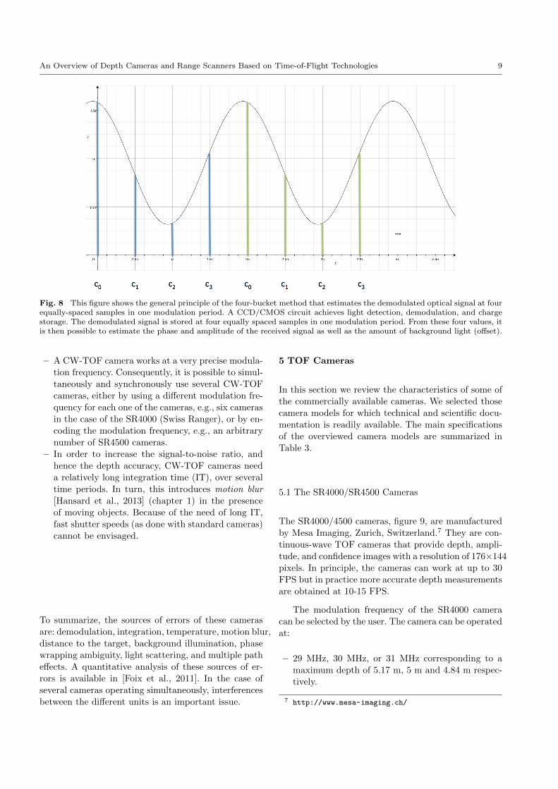
5.1 The SR4000/SR4500 Cameras

The SR4000/4500 cameras, figure 9, are manufactured

by Mesa Imaging, Zurich, Switzerland.7 They are con-

tinuous-wave TOF cameras that provide depth, ampli-

tude, and confidence images with a resolution of 176×144

pixels. In principle, the cameras can work at up to 30

FPS but in practice more accurate depth measurements

are obtained at 10-15 FPS.

The modulation frequency of the SR4000 camera

can be selected by the user. The camera can be operated

at:

– 29 MHz, 30 MHz, or 31 MHz corresponding to a

maximum depth of 5.17 m, 5 m and 4.84 m respec-

tively.

7 http://www.mesa-imaging.ch/


Fig. 9 The SR4000 (left) and SR4500 (right) CW-TOF cam-eras manufactured by Mesa Imaging.

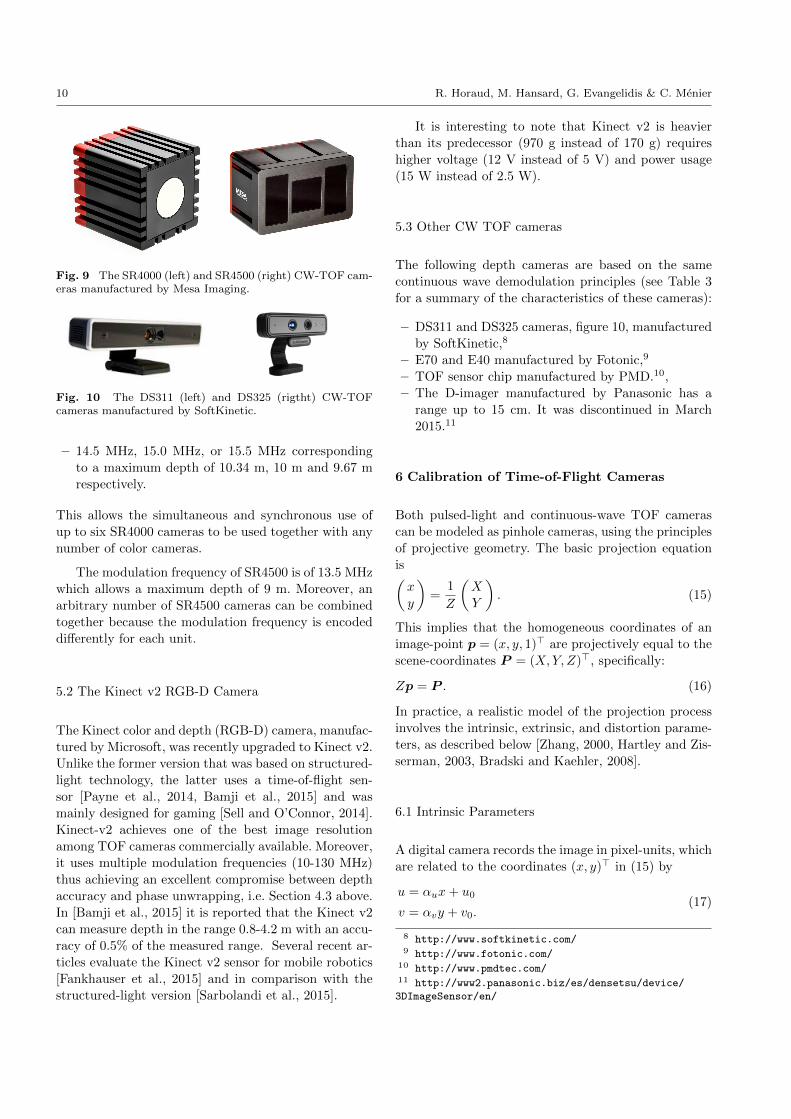
Fig. 10 The DS311 (left) and DS325 (rigtht) CW-TOFcameras manufactured by SoftKinetic.

– 14.5 MHz, 15.0 MHz, or 15.5 MHz corresponding

to a maximum depth of 10.34 m, 10 m and 9.67 m

respectively.

This allows the simultaneous and synchronous use of

up to six SR4000 cameras to be used together with any

number of color cameras.

The modulation frequency of SR4500 is of 13.5 MHz

which allows a maximum depth of 9 m. Moreover, an

arbitrary number of SR4500 cameras can be combined

together because the modulation frequency is encoded

differently for each unit.

5.2 The Kinect v2 RGB-D Camera

The Kinect color and depth (RGB-D) camera, manufac-

tured by Microsoft, was recently upgraded to Kinect v2.

Unlike the former version that was based on structured-

light technology, the latter uses a time-of-flight sen-

sor [Payne et al., 2014, Bamji et al., 2015] and was

mainly designed for gaming [Sell and O’Connor, 2014].

Kinect-v2 achieves one of the best image resolution

among TOF cameras commercially available. Moreover,

it uses multiple modulation frequencies (10-130 MHz)

thus achieving an excellent compromise between depth

accuracy and phase unwrapping, i.e. Section 4.3 above.

In [Bamji et al., 2015] it is reported that the Kinect v2

can measure depth in the range 0.8-4.2 m with an accu-

racy of 0.5% of the measured range. Several recent ar-

ticles evaluate the Kinect v2 sensor for mobile robotics

[Fankhauser et al., 2015] and in comparison with the

structured-light version [Sarbolandi et al., 2015].

It is interesting to note that Kinect v2 is heavier

than its predecessor (970 g instead of 170 g) requires

higher voltage (12 V instead of 5 V) and power usage

(15 W instead of 2.5 W).

5.3 Other CW TOF cameras

The following depth cameras are based on the same

continuous wave demodulation principles (see Table 3

for a summary of the characteristics of these cameras):

– DS311 and DS325 cameras, figure 10, manufactured

by SoftKinetic,8

– E70 and E40 manufactured by Fotonic,9

– TOF sensor chip manufactured by PMD.10,

– The D-imager manufactured by Panasonic has a

range up to 15 cm. It was discontinued in March

2015.11

6 Calibration of Time-of-Flight Cameras

Both pulsed-light and continuous-wave TOF cameras

can be modeled as pinhole cameras, using the principles

of projective geometry. The basic projection equation

is(x

y

)=

1

Z

(X

Y

). (15)

This implies that the homogeneous coordinates of an

image-point p = (x, y, 1)> are projectively equal to the

scene-coordinates P = (X,Y, Z)>, specifically:

Zp = P . (16)

In practice, a realistic model of the projection process

involves the intrinsic, extrinsic, and distortion parame-

ters, as described below [Zhang, 2000, Hartley and Zis-

serman, 2003, Bradski and Kaehler, 2008].

6.1 Intrinsic Parameters

A digital camera records the image in pixel-units, which

are related to the coordinates (x, y)> in (15) by

u = αux+ u0

v = αvy + v0.(17)

8 http://www.softkinetic.com/9 http://www.fotonic.com/

10 http://www.pmdtec.com/11 http://www2.panasonic.biz/es/densetsu/device/

3DImageSensor/en/


Camera Resolution Range Mult. cameras FOV Max FPS Illumination Indoor/out

SR4000 176×144 0−5 or 0−10 m 6 cameras 43◦ × 34◦ 30 LED yes/noSR4500 176×144 0−9 m many cameras 43◦ × 34◦ 30 LED yes/noDS311 160×120 0.15−1 or 1.5−4.5 m not specified 57◦ × 42◦ 60 LED yes/noDS325 320×240 0.15−1 m not specified 74◦ × 58◦ 60 diffused laser yes/noE70 160×120 0.1−10 m 4 cameras 70◦ × 53◦ 52 LED yes/yesE40 160×120 0.1−10 m 4 cameras 45◦ × 34◦ 52 LED yes/yesKinect v2 512×424 0.8−4.2 m not specified 70◦ × 60◦ 30 LED yes/no

Table 3 This table summarizes the main features of commercially available CW TOF cameras. The accuracy of the depthmeasurements announced by the manufacturers are not reported in this table as the precision of the measurements depend ona lot of factors, such as the surface properties of the scene objects, illumination conditions, frame rate, etc.

In these equations we have the following intrinsic pa-

rameters:

– Horizontal and vertical factors, αu and αv, which

encode the change of scale, multiplied by the focal

length.

– The image center, or principal point, expressed in

pixel units: (u0, v0).

Alternatively, the intrinsic transformation (17) can be

expressed in matrix form, q = Ap where q = (u, v, 1)

are pixel coordinates, and the 3×3 matrix A is defined

as

A =

αu 0 u00 αv v00 0 1

. (18)

Hence it is possible to express the direction of a visual

ray, in camera coordinates, as

p = A−1q. (19)

A TOF camera further allows the 3D position of point

P to be estimated, as follows. Observe from equation

(16) that the Euclidean norms of P and p are propor-

tional:

‖P ‖ = Z‖p‖. (20)

The TOF camera measures the distance d from the 3D

point P to the optical center,12 so d = ‖P ‖. Hence the

Z coordinate of the observed point is

Z =‖P ‖‖p‖

=d

‖A−1q‖. (21)

We can therefore obtain the 3D coordinates of the ob-

served point, by combining (16) and (19), to give

P =d

‖A−1q‖A−1q. (22)

Note that the point is recovered in the camera coordi-

nate system; the transformation to a common ‘world’

coordinate system is explained in the following section.

12 In practice it measures the distance to the image sensorand we assume that the offset between the optical center andthe sensor is small

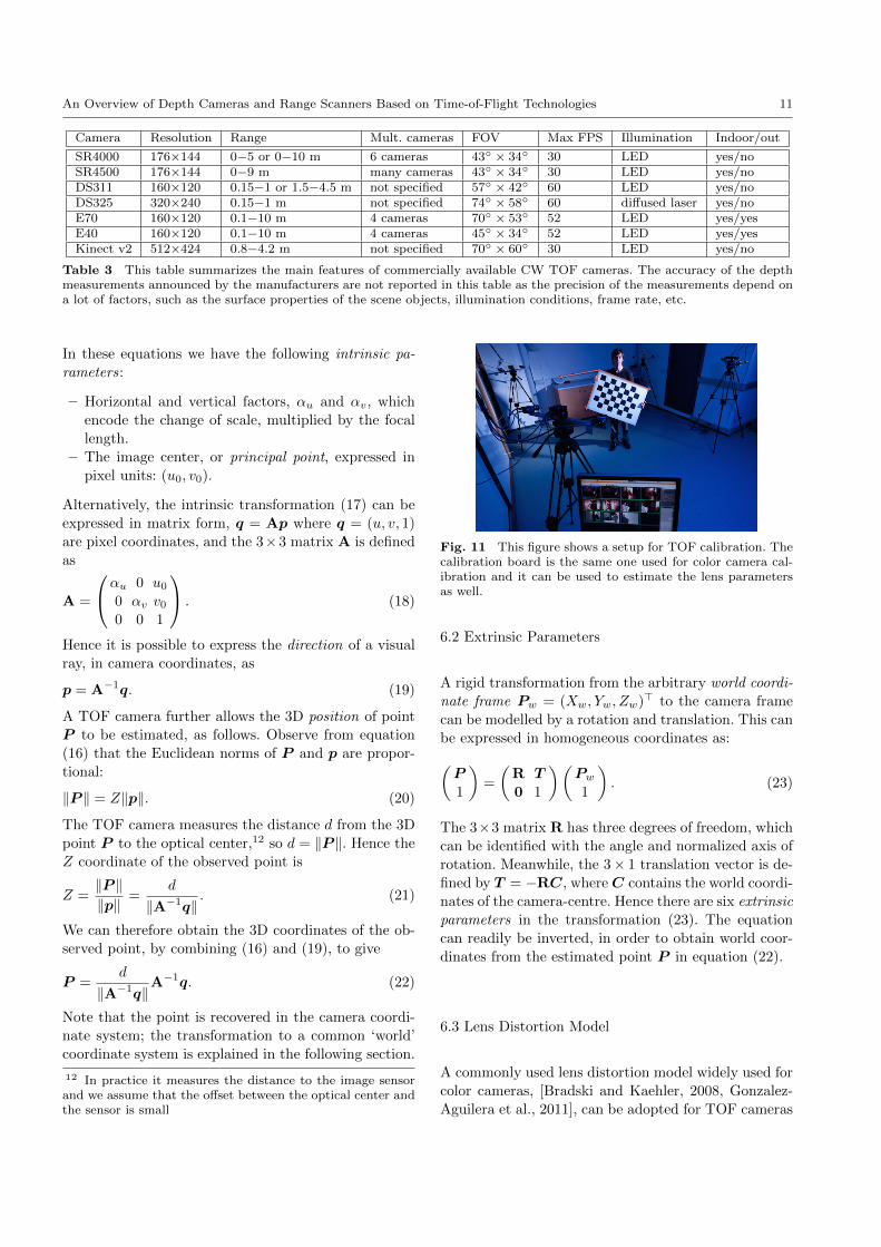
Fig. 11 This figure shows a setup for TOF calibration. Thecalibration board is the same one used for color camera cal-ibration and it can be used to estimate the lens parametersas well.

6.2 Extrinsic Parameters

A rigid transformation from the arbitrary world coordi-

nate frame Pw = (Xw, Yw, Zw)> to the camera frame

can be modelled by a rotation and translation. This can

be expressed in homogeneous coordinates as:(P

1

)=

(R T

0 1

)(Pw1

). (23)

The 3×3 matrix R has three degrees of freedom, which

can be identified with the angle and normalized axis of

rotation. Meanwhile, the 3× 1 translation vector is de-

fined by T = −RC, where C contains the world coordi-

nates of the camera-centre. Hence there are six extrinsic

parameters in the transformation (23). The equation

can readily be inverted, in order to obtain world coor-

dinates from the estimated point P in equation (22).

6.3 Lens Distortion Model

A commonly used lens distortion model widely used for

color cameras, [Bradski and Kaehler, 2008, Gonzalez-

Aguilera et al., 2011], can be adopted for TOF cameras


as well: the observed distorted point (xl, yl) results from

the displacement of (x, y) according to:(xlyl

)= lρ(r)

(x

y

)+ lτ (x, y) (24)

where lρ(r) is a scalar radial function of r =√x2 + y2,

and lτ (x, y) is a vector tangential component. These are

commonly defined by polynomial functions

lρ(r) = 1 + ρ1r2 + ρ2r

4 and (25)

lτ (x, y) =

[2xy r2 + 2x2

r2 + 2y2 2xy

](τ1τ2

)(26)

such that the complete parameter-vector is [ρ1 ρ2 τ1 τ2].

The images can be undistorted, by numerically invert-

ing (26), given the lens and intrinsic parameters. The

projective linear model, described in sections (6.1–6.2),

can then be used to describe the complete imaging pro-

cess, with respect to the undistorted images.

It should also be noted, in the case of TOF cameras,

that the outgoing infrared signal is subject to optical ef-

fects. In particular, there is a radial attenuation, which

results in strong vignetting of the intensity image. This

can be modeled by a bivariate polynomial, if a full pho-

tometric calibration is required [Lindner et al., 2010,

Hertzberg and Frese, 2014].

6.4 Depth Distortion Models

TOF depth estimates are also subject to systematic

nonlinear distortions, particulalry due to deviation of

the emitted signal from the ideal model described in

Section 4.1. This results in ‘wiggling’ error of the av-

erage distance estimates, with respect to the true dis-

tance [Foix et al., 2011, Fursattel et al., 2016]. Because

this error is systematic, it can be removed by reference

to a precomputed look-up table [Kahlmann et al., 2006].

Another possibility is to learn a mapping between raw

depth values, estimated by the sensor, and corrected

values. This mapping can be performed using regres-

sion techniques applied to carefully calibrated data. A

random regression forest is used in [Ferstl et al., 2015] to

optimize the depth measurements supplied by the cam-

era. A kernel regression method based on a Gaussian

kernel is used in [Kuznetsova and Rosenhahn, 2014] to

estimate the depth bias at each pixel. Below we describe

an efficient approach, which exploits the smoothness of

the error, and which uses a B-spline regression [Lindner

et al., 2010] of the form:

d′(x, y) = d(x, y)−n∑i

βiBi,3(d(x, y)

)(27)

where d′(x, y) is the corrected depth. The spline basis-

functions Bi,3(d) are located at n evenly-spaced depth

control-points di. The coefficients βi, i = 1, . . . , n can

be estimated by least-squares optimization, given the

known target-depths. The total number of coefficients

n depends on the number of known depth-planes in the

calibration procedure.

6.5 Practical Considerations

To summarize, the TOF camera parameters are com-

posed of the pinhole camera model, namely the pa-

rameters αu, αv, u0, v0 and the lens distortion parame-

ters, namely ρ1, ρ2, τ1, τ2. Standard camera calibration

methods can be used with TOF cameras, in particular

with CW-TOF cameras because they provide an am-

plitude+offset image, i.e. Section 4, together with the

depth image: Standard color-camera calibration meth-

ods, e.g. OpenCV packages, can be applied to the am-

plitude+offset image. However, the low-resolution of

the TOF images implies specific image processing tech-

niques, such as [Hansard et al., 2014, Kuznetsova and

Rosenhahn, 2014]. As en example, Fig. 12 shows the

depth and amplitude images of a calibration pattern

gathered with the SR4000 camera. Here the standard

corner detection method was replaced with the detec-

tion of two pencils of lines that are optimally fitted to

the OpenCV calibration pattern.

TOF-specific calibration procedures can also be per-

formed, such as the depth-wiggling correction [Lindner

et al., 2010, Kuznetsova and Rosenhahn, 2014, Ferstl

et al., 2015]. A variety of TOF calibration methods canbe found in a recent book [Grzegorzek et al., 2013]. A

comparative study of several TOF cameras based on an

error analysis was also proposed [Fursattel et al., 2016].

One should however be aware of the fact that depth

measurement errors may be quite difficult to predict

due to the unknown material properties of the sensed

objects and to the complexity of the scene. In the case

of a scene composed of complex objects, multiple-path

distortion may occur, due to the interaction between

the emitted light and the scene objects, e.g. the emitted

light is backscattered more than once. Techniques for

removing multiple-path distortions were recently pro-

posed [Freedman et al., 2014, Son et al., 2016].

7 Combining Multiple TOF and Color Cameras

In addition to the image and depth-calibration proce-

dures described in section 6, it is often desirable to


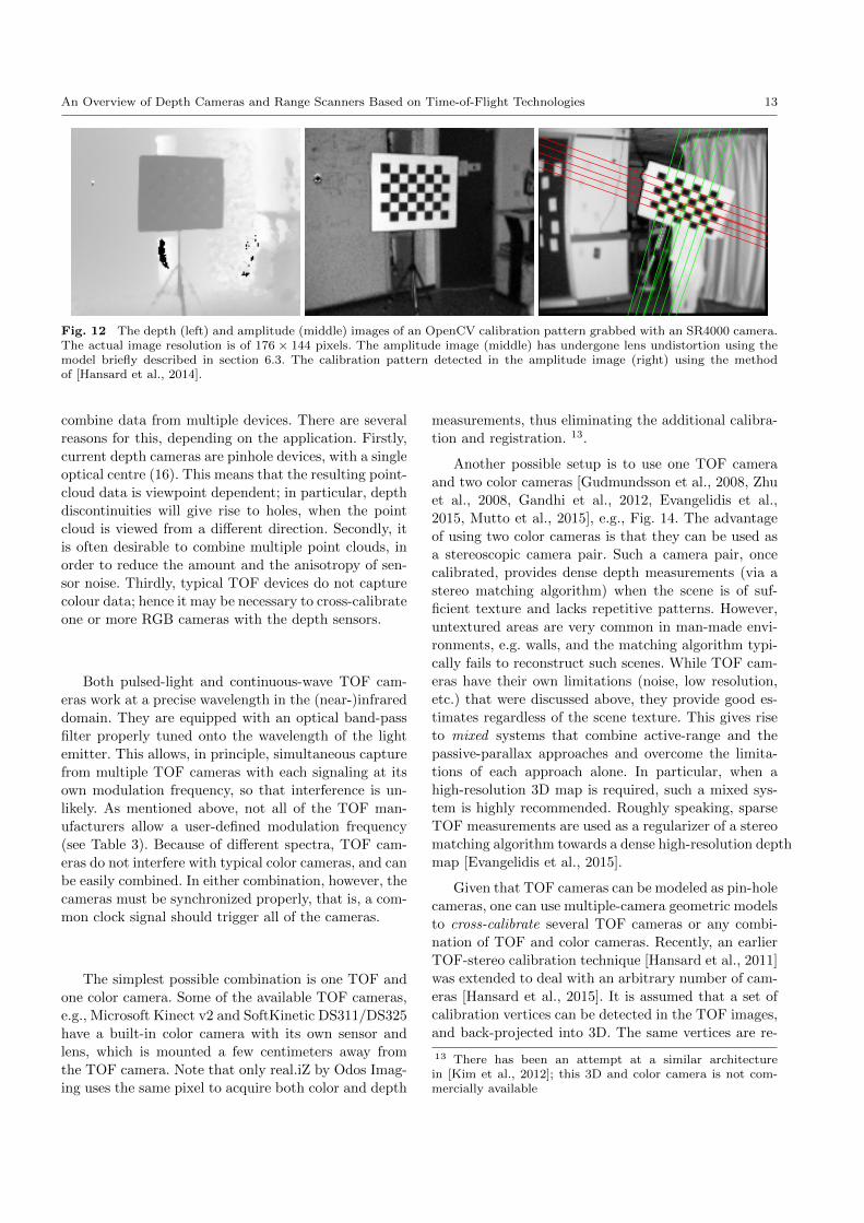
Fig. 12 The depth (left) and amplitude (middle) images of an OpenCV calibration pattern grabbed with an SR4000 camera.The actual image resolution is of 176 × 144 pixels. The amplitude image (middle) has undergone lens undistortion using themodel briefly described in section 6.3. The calibration pattern detected in the amplitude image (right) using the methodof [Hansard et al., 2014].

combine data from multiple devices. There are several

reasons for this, depending on the application. Firstly,

current depth cameras are pinhole devices, with a single

optical centre (16). This means that the resulting point-

cloud data is viewpoint dependent; in particular, depth

discontinuities will give rise to holes, when the point

cloud is viewed from a different direction. Secondly, it

is often desirable to combine multiple point clouds, in

order to reduce the amount and the anisotropy of sen-

sor noise. Thirdly, typical TOF devices do not capture

colour data; hence it may be necessary to cross-calibrate

one or more RGB cameras with the depth sensors.

Both pulsed-light and continuous-wave TOF cam-

eras work at a precise wavelength in the (near-)infrared

domain. They are equipped with an optical band-pass

filter properly tuned onto the wavelength of the light

emitter. This allows, in principle, simultaneous capture

from multiple TOF cameras with each signaling at its

own modulation frequency, so that interference is un-

likely. As mentioned above, not all of the TOF man-

ufacturers allow a user-defined modulation frequency

(see Table 3). Because of different spectra, TOF cam-

eras do not interfere with typical color cameras, and can

be easily combined. In either combination, however, the

cameras must be synchronized properly, that is, a com-

mon clock signal should trigger all of the cameras.

The simplest possible combination is one TOF and

one color camera. Some of the available TOF cameras,

e.g., Microsoft Kinect v2 and SoftKinetic DS311/DS325

have a built-in color camera with its own sensor and

lens, which is mounted a few centimeters away from

the TOF camera. Note that only real.iZ by Odos Imag-

ing uses the same pixel to acquire both color and depth

measurements, thus eliminating the additional calibra-

tion and registration. 13.

Another possible setup is to use one TOF camera

and two color cameras [Gudmundsson et al., 2008, Zhu

et al., 2008, Gandhi et al., 2012, Evangelidis et al.,

2015, Mutto et al., 2015], e.g., Fig. 14. The advantage

of using two color cameras is that they can be used as

a stereoscopic camera pair. Such a camera pair, once

calibrated, provides dense depth measurements (via a

stereo matching algorithm) when the scene is of suf-

ficient texture and lacks repetitive patterns. However,

untextured areas are very common in man-made envi-

ronments, e.g. walls, and the matching algorithm typi-

cally fails to reconstruct such scenes. While TOF cam-

eras have their own limitations (noise, low resolution,

etc.) that were discussed above, they provide good es-

timates regardless of the scene texture. This gives rise

to mixed systems that combine active-range and the

passive-parallax approaches and overcome the limita-

tions of each approach alone. In particular, when a

high-resolution 3D map is required, such a mixed sys-

tem is highly recommended. Roughly speaking, sparse

TOF measurements are used as a regularizer of a stereo

matching algorithm towards a dense high-resolution depth

map [Evangelidis et al., 2015].

Given that TOF cameras can be modeled as pin-hole

cameras, one can use multiple-camera geometric models

to cross-calibrate several TOF cameras or any combi-

nation of TOF and color cameras. Recently, an earlier

TOF-stereo calibration technique [Hansard et al., 2011]

was extended to deal with an arbitrary number of cam-

eras [Hansard et al., 2015]. It is assumed that a set of

calibration vertices can be detected in the TOF images,

and back-projected into 3D. The same vertices are re-

13 There has been an attempt at a similar architecturein [Kim et al., 2012]; this 3D and color camera is not com-mercially available


constructed via stereo-matching, using the high resolu-

tion RGB cameras. Ideally, the two 3D reconstructions

could be aligned by a rigid 3D transformation; how-

ever, this is not true in practice, owing to calibration

uncertainty in both the TOF and RGB cameras. Hence

a more general alignment, via a 3D projective trans-

formation, was derived. This approach has several ad-

vantages, including a straightforward SVD calibration

procedure, which can be refined by photogrammetric

bundle-adjustment routines. An alternative approach,

initialized by the factory calibration of the TOF cam-

era, is described by [Jung et al., 2014].

A different cross-calibration method can be devel-

oped from the constraint that depth points lie on cali-

bration planes, where the latter are also observed by the

colour camera [Zhang and Zhang, 2011]. This method,

however, does not provide a framework for calibrating

the intrinsic (section 6.1) or lens (section 6.3) parame-

ters of the depth camera. A related method, which does

include distortion correction, has been demonstrated

for Kinect v1 [Herrera et al., 2012].

Finally, a more object-based approach can be adopted,

in which dense overlapping depth-scans are merged to-

gether in 3D. This approach, which is ideally suited

to handheld (or robotic) scanning, has been applied to

both Kinect v1 [Newcombe et al., 2011] and TOF cam-

eras [Cui et al., 2013].

8 Conclusions

Time of flight is a remote-sensing technology that esti-

mates range (depth) by illuminating an object with a

laser or with a photodiode and by measuring the travel

time from the emitter to the object and back to the de-

tector. Two technologies are available today, one based

on pulsed-light and the second based on continuous-

wave modulation. Pulsed-light sensors measure directly

the pulse’s total trip time and use either rotating mir-

rors (LIDAR) or a light diffuser (Flash LIDAR) to pro-

duce a two-dimensional array of range values. Continuous-

wave (CW) sensors measure the phase difference be-

tween the emitted and received signals and the phase

is estimated via demodulation. LIDAR cameras usually

operate outdoor and their range can be up to a few kilo-

meters. CW cameras usually operate indoor and they

allow for short-distance measurements only, namely up

to 10 meters. Depth estimation based on phase mea-

surement suffer from an intrinsic phase-wrapping ambi-

guity. Higher the modulation frequency, more accurate

the measurement and shorter the range.

Generally speaking, the spatial resolution of these

sensors is a few orders of magnitude (10 to 100) less

than video cameras. This is mainly due to the need

to capture sufficient backscattered light. The depth ac-

curacy depends on multiple factors and can vary from

a few centimeters up to several meters. TOF cameras

can be modeled as pinhole cameras and therefore one

can use standard camera calibration techniques (distor-

tion, intrinsic and extrinsic parameters). One advantage

of TOF cameras over depth sensors based on struc-

tured light and triangulation, is that the former pro-

vides an amplitude+offset image. The amplitude+offset

and depth images are gathered by the same and unique

sensor, hence one can use camera calibration techniques

routinely used with color sensors to calibrate TOF cam-

eras. This is not the case with triangulation-based range

sensors for which special-purpose calibration techniques

must be used. Moreover, the relative orientation be-

tween the infrared camera and the color camera must

be estimated as well.

TOF cameras and TOF range scanners are used for

a wide range of applications, from multimedia user in-

terfaces to autonomous vehicle navigation and plane-

tary/space exploration. More precisely:

– Pulsed-light devices, such as the Velodyne, Toyota,

and Advanced Scientific Concepts LIDARs can be

used under adverse outdoor lighting conditions, which

is not the case with continuous-wave systems. These

LIDARs are the systems of choice for autonomous

vehicle driving and for robot navigation (obstacle,

car, and pedestrian detection, road following, etc.).The Toyota LIDAR scanner is a laboratory proto-

type, at the time of writing.

– The 3D Flash LIDAR cameras manufactured by Ad-

vanced Scientific Concepts have been developed in

collaboration with NASA for the purpose of planet

landing [Amzajerdian et al., 2011]. They are com-

mercially available.

– The SR4000/45000 cameras are used for industrial

and for multimedia applications. Although they have

limited image resolution, these cameras can be eas-

ily combined together into multiple TOF and cam-

era systems. They are commercially available.

– The Kinect v2, SoftKinetic, Basler and Fotonic cam-

eras are used for multimedia and robotic applica-

tions. They are commercially available, some of them

at a very affordable price. Additionally, some of these

sensors integrate an additional color camera which is

internally synchronized with the TOF camera, thus

yielding RGB-D data. Nevertheless, one shortcom-

ing is that they cannot be easily externally synchro-


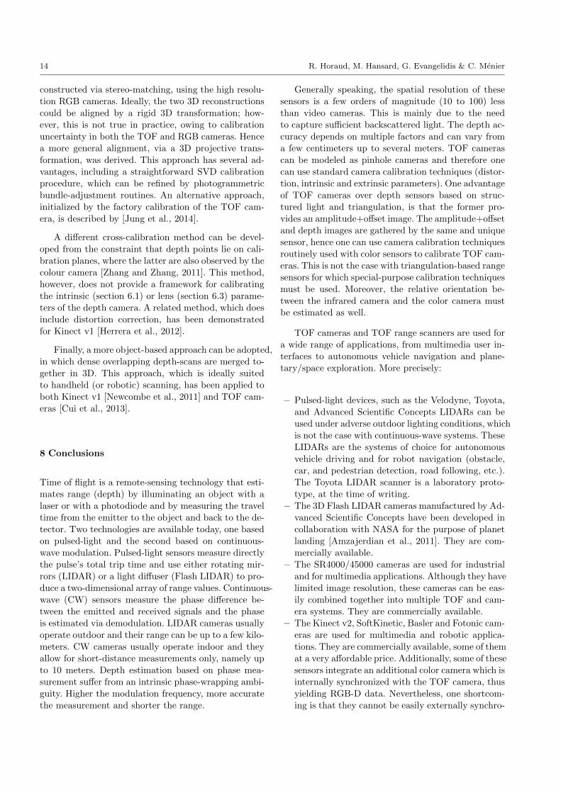
Fig. 13 A single system (left), comprising a time-of-flight camera in the centre, plus a pair of ordinary color cameras. Several(four) such systems can be combined together and calibrated in order to be used for 3D scene reconstruction (right).

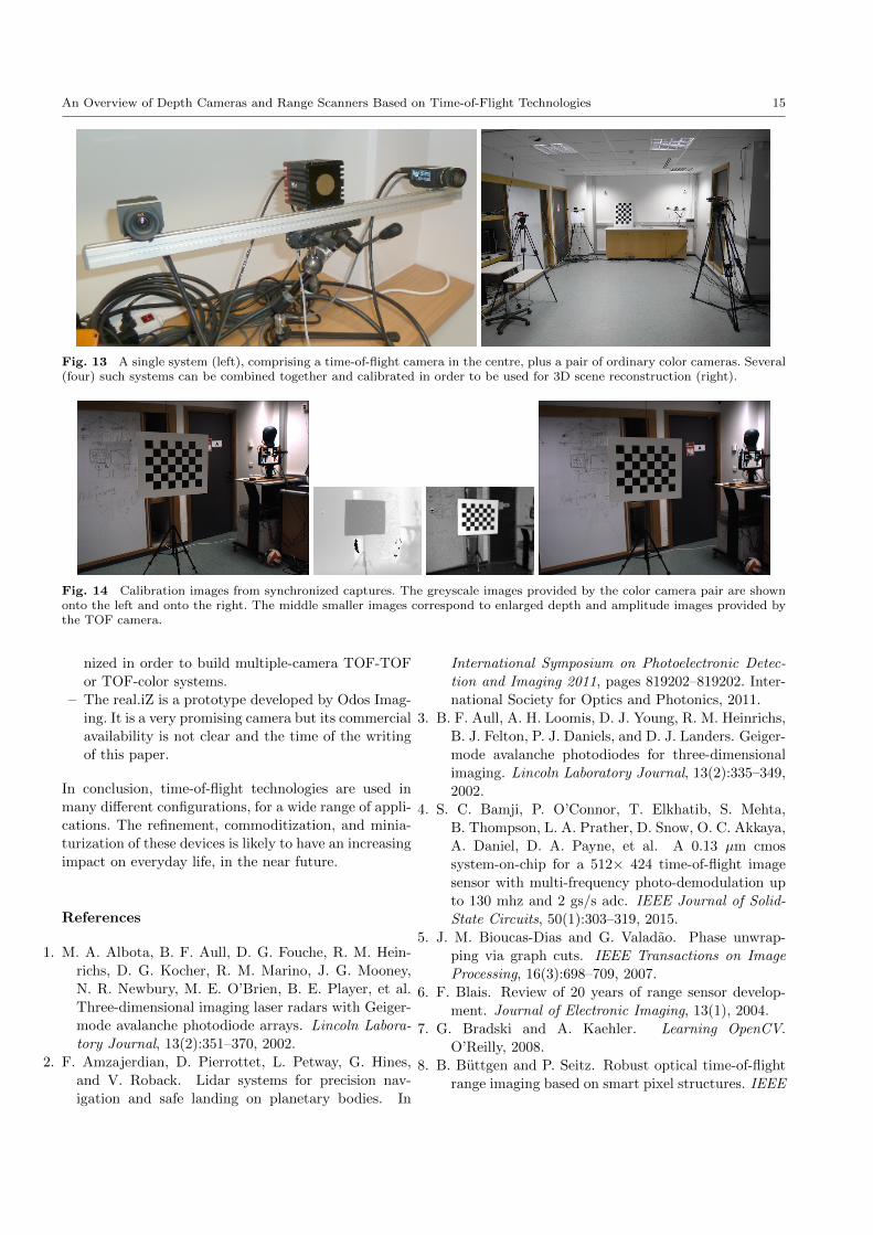
Fig. 14 Calibration images from synchronized captures. The greyscale images provided by the color camera pair are shownonto the left and onto the right. The middle smaller images correspond to enlarged depth and amplitude images provided bythe TOF camera.

nized in order to build multiple-camera TOF-TOF

or TOF-color systems.

– The real.iZ is a prototype developed by Odos Imag-

ing. It is a very promising camera but its commercial

availability is not clear and the time of the writing

of this paper.

In conclusion, time-of-flight technologies are used in

many different configurations, for a wide range of appli-

cations. The refinement, commoditization, and minia-

turization of these devices is likely to have an increasing

impact on everyday life, in the near future.

References

1. M. A. Albota, B. F. Aull, D. G. Fouche, R. M. Hein-

richs, D. G. Kocher, R. M. Marino, J. G. Mooney,

N. R. Newbury, M. E. O’Brien, B. E. Player, et al.

Three-dimensional imaging laser radars with Geiger-

mode avalanche photodiode arrays. Lincoln Labora-

tory Journal, 13(2):351–370, 2002.

2. F. Amzajerdian, D. Pierrottet, L. Petway, G. Hines,

and V. Roback. Lidar systems for precision nav-

igation and safe landing on planetary bodies. In

International Symposium on Photoelectronic Detec-

tion and Imaging 2011, pages 819202–819202. Inter-

national Society for Optics and Photonics, 2011.

3. B. F. Aull, A. H. Loomis, D. J. Young, R. M. Heinrichs,

B. J. Felton, P. J. Daniels, and D. J. Landers. Geiger-

mode avalanche photodiodes for three-dimensional

imaging. Lincoln Laboratory Journal, 13(2):335–349,

2002.

4. S. C. Bamji, P. O’Connor, T. Elkhatib, S. Mehta,

B. Thompson, L. A. Prather, D. Snow, O. C. Akkaya,

A. Daniel, D. A. Payne, et al. A 0.13 µm cmos

system-on-chip for a 512× 424 time-of-flight image

sensor with multi-frequency photo-demodulation up

to 130 mhz and 2 gs/s adc. IEEE Journal of Solid-

State Circuits, 50(1):303–319, 2015.

5. J. M. Bioucas-Dias and G. Valadao. Phase unwrap-

ping via graph cuts. IEEE Transactions on Image

Processing, 16(3):698–709, 2007.

6. F. Blais. Review of 20 years of range sensor develop-

ment. Journal of Electronic Imaging, 13(1), 2004.

7. G. Bradski and A. Kaehler. Learning OpenCV.

O’Reilly, 2008.

8. B. Buttgen and P. Seitz. Robust optical time-of-flight

range imaging based on smart pixel structures. IEEE


Transactions on Circuits and Systems I: Regular Pa-

pers, 55(6):1512–1525, 2008.

9. O. Choi and S. Lee. Wide range stereo time-of-flight

camera. In Proceedings IEEE International Confer-

ence on Image Processing, 2012.

10. O. Choi, H. Lim, B. Kang, Y. S. Kim, K. Lee, J. D. K.

Kim, and C. Y. Kim. Range unfolding for time-of-

flight depth cameras. In Proceedings IEEE Interna-

tional Conference on Image Processing, 2010.

11. S. Cova, A. Longoni, and A. Andreoni. Towards

picosecond resolution with single-photon avalanche

diodes. Review of Scientific Instruments, 52(3):408–

412, 1981.

12. Y. Cui, S. Schuon, S. Thrun, D. Stricker, and

C. Theobalt. Algorithms for 3d shape scanning with a

depth camera. IEEE Transactions on Pattern Analy-

sis and Machine Intelligence, 35(5):1039–1050, 2013.

13. D. Droeschel, D. Holz, and S. Behnke. Probabilistic

phase unwrapping for time-of-flight cameras. In Joint

41st International Symposium on Robotics and 6th

German Conference on Robotics, 2010a.

14. D. Droeschel, D. Holz, and S. Behnke. Multifrequency

phase unwrapping for time-of-flight cameras. In

IEEE/RSJ International Conference on Intelligent

Robots and Systems, 2010b.

15. G. D. Evangelidis, M. Hansard, and R. Horaud. Fusion

of Range and Stereo Data for High-Resolution Scene-

Modeling. IEEE Trans. PAMI, 37(11):2178 – 2192,

2015.

16. P. Fankhauser, M. Bloesch, D. Rodriguez, R. Kaest-

ner, M. Hutter, and R. Siegwart. Kinect v2 for Mo-

bile Robot Navigation: Evaluation and Modeling. In

International Conference on Advanced Robotics, Is-

tanbul, Turkey, July 2015.

17. D. Ferstl, C. Reinbacher, G. Riegler, M. Ruther, and

H. Bischof. Learning depth calibration of time-of-

flight cameras. Technical report, Graz University of

Technology, 2015.

18. S. Foix, G. Alenya, and C. Torras. Lock-in Time-of-

Flight (ToF) Cameras: A Survey. IEEE Sensors, 11

(9):1917–1926, Sept 2011.

19. D. Freedman, Y. Smolin, E. Krupka, I. Leichter, and

M. Schmidt. Sra: Fast removal of general multipath

for tof sensors. In European Conference on Computer

Vision, pages 234–249. Springer, 2014.

20. P. Fursattel, S. Placht, C. Schaller, M. Balda, H. Hof-

mann, A. Maier, and C. Riess. A comparative er-

ror analysis of current time-of-flight sensors. IEEE

Transactions on Computational Imaging, 2(1):27 –

41, 2016.

21. V. Gandhi, J. Cech, and R. Horaud. High-resolution

depth maps based on TOF-stereo fusion. In IEEE In-

ternational Conference on Robotics and Automation,

pages 4742–4749, 2012.

22. D. C. Ghiglia and L. A. Romero. Robust two-

dimensional weighted and unweighted phase unwrap-

ping that uses fast transforms and iterative methods.

Journal of Optical Society of America A, 11(1):107–

117, 1994.

23. C. Glennie. Rigorous 3D error analysis of kine-

matic scanning LIDAR systems. Journal of Applied

Geodesy, 1(3):147–157, 2007.

24. C. Glennie and D. D. Lichti. Static calibration and

analysis of the velodyne hdl-64e s2 for high accuracy

mobile scanning. Remote Sensing, 2(6):1610–1624,

2010.

25. C. Glennie and D. D. Lichti. Temporal stability of

the velodyne hdl-64e s2 scanner for high accuracy

scanning applications. Remote Sensing, 3(3):539–

553, 2011.

26. D. Gonzalez-Aguilera, J. Gomez-Lahoz, and

P. Rodriguez-Gonzalvez. An automatic approach for

radial lens distortion correction from a single image.

IEEE Sensors, 11(4):956–965, 2011.

27. M. Grzegorzek, C. Theobalt, R. Koch, and A. Kolb.

Time-of-Flight and Depth Imaging. Sensors, Algo-

rithms and Applications, volume 8200. Springer,

2013.

28. Sigurjon Arni Gudmundsson, Henrik Aanaes, and Ras-

mus Larsen. Fusion of stereo vision and time-of-flight

imaging for improved 3D estimation. Int. J. Intell.

Syst. Technol. Appl., 5(3/4), 2008.

29. M. Hansard, R. Horaud, M. Amat, and S.K. Lee.

Projective alignment of range and parallax data.

In IEEE Computer Vision and Pattern Recognition,

pages 3089–3096, 2011.

30. M. Hansard, S. Lee, O. Choi, and R. Horaud. Time-

of-Flight Cameras: Principles, Methods and Applica-

tions. Springer, 2013.

31. M. Hansard, R. Horaud, M. Amat, and G. Evangelidis.

Automatic detection of calibration grids in time-of-

flight images. Computer Vision and Image Under-

standing, 121:108–118, 2014.

32. M. Hansard, G. Evangelidis, Q. Pelorson, and R. Ho-

raud. Cross-calibration of time-of-flight and colour

cameras. Computer Vision and Image Understand-

ing, 134:105–115, May 2015.

33. R. Hartley and A. Zisserman. Multiple View Geometry

in Computer Vision. Cambridge University Press,

2003.

34. D.C. Herrera, J. Kannala, and J. Heikila. Joint Depth

and Color Camera Calibration with Distortion Cor-

rection. IEEE Trans. PAMI, 34(10):2058–2064, 2012.

35. Christoph Hertzberg and Udo Frese. Detailed modeling

and calibration of a time-of-flight camera. In ICINCO

2014 - Proc. International Conference on Informatics


in Control, Automation and Robotics, pages 568–579,

2014.

36. J. Jung, J-Y. Lee, Y. Jeong, and I.S. Kweon. Time-of-

flight sensor calibration for a color and depth camera

pair. IEEE Transactions on Pattern Analysis and

Machine Intelligence, 2014.

37. T. Kahlmann, F. Remondino B, and H. Ingensand.

Calibration for increased accuracy of the range imag-

ing camera swissranger. In ISPRS Archives, pages

136–141, 2006.

38. S.-J. Kim, J. D. K. Kim, B. Kang, and K. Lee. A

CMOS image sensor based on unified pixel architec-

ture with time-division multiplexing scheme for color

and depth image acquisition. IEEE Journal of Solid-

State Circuits, 47(11):2834–2845, 2012.

39. A. Kuznetsova and B. Rosenhahn. On calibration of a

low-cost time-of-flight camera. In ECCV Workshops,

pages 415–427, 2014.

40. R. Lange and P. Seitz. Solid-state time-of-flight range

camera. IEEE Journal of Quantum Electronics, 37

(3):390–397, 2001.

41. M. Lindner, I. Schiller, A. Kolb, and R. Koch. Time-

of-flight sensor calibration for accurate range sensing.

Computer Vision and Image Understanding, 114(12):

1318–1328, 2010.

42. S. H. McClure, M. J. Cree, A. A. Dorrington, and

A. D. Payne. Resolving depth-measurement ambigu-

ity with commercially available range imaging cam-

eras. In Image Processing: Machine Vision Applica-

tions III, 2010.

43. C.D. Mutto, P. Zanuttigh, and G.M. Cortelazzo. Prob-

abilistic ToF and Stereo Data Fusion Based on Mixed

Pixels Measurement Models. IEEE Trans. PAMI, 37

(11):2260 – 2272, 2015.

44. R. A. Newcombe, S. Izadi, O. Hilliges, D. Molyneaux,

D. Kim, A. J. Davison, P. Kohli, J. Shotton,

S. Hodges, and A. Fitzgibbon. Kinectfusion: Real-

time dense surface mapping and tracking. In ISMAR,

2011.

45. C. Niclass, A. Rochas, P.-A. Besse, and E. Charbon.

Design and characterization of a CMOS 3-D im-

age sensor based on single photon avalanche diodes.

IEEE Journal of Solid-State Circuits, 40(9):1847–

1854, 2005.

46. C. Niclass, C. Favi, T. Kluter, M. Gersbach, and

E. Charbon. A 128×128 single-photon image sen-

sor with column-level 10-bit time-to-digital converter

array. IEEE Journal of Solid-State Circuits, 43(12):

2977–2989, 2008.

47. C. Niclass, M. Soga, H. Matsubara, S. Kato, and

M. Kagami. A 100-m range 10-frame/s 340 96-pixel

time-of-flight depth sensor in 0.18-CMOS. IEEE

Journal of Solid-State Circuits, 48(2):559–572, 2013.

48. S. Oprisescu, D. Falie, M. Ciuc, and V. Buzuloiu. Mea-

surements with TOF cameras and their necessary

corrections. In IEEE International Symposium on

Signals, Circuits & Systems, 2007.

49. A. Payne, A. Daniel, A. Mehta, B. Thompson, C. S.

Bamji, D. Snow, H. Oshima, L. Prather, M. Fen-

ton, L. Kordus, et al. A 512×424 CMOS 3D time-

of-flight image sensor with multi-frequency photo-

demodulation up to 130MHz and 2GS/s ADC. In

IEEE International Solid-State Circuits Conference

Digest of Technical Papers, pages 134–135. IEEE,

2014.

50. A. D. Payne, A. P. P. Jongenelen, A. A. Dorrington,

M. J. Cree, and D. A. Carnegie. Multiple frequency

range imaging to remove measurement ambiguity. In

9th Conference on Optical 3-D Measurement Tech-

niques, 2009.

51. F. Remondino and D. Stoppa, editors. TOF Range-

Imaging Cameras. Springer, 2013.

52. H. Sarbolandi, D. Lefloch, and A. Kolb. Kinect range

sensing: Structured-light versus time-of-flight Kinect.

CVIU, 139:1–20, October 2015.

53. B. Schwarz. Mapping the world in 3D. Nature Pho-

tonics, 4(7):429–430, 2010.

54. J. Sell and P. O’Connor. The Xbox one system on a

chip and Kinect sensor. IEEE Micro, 32(2):44–53,

2014.

55. K. Son, M.-Y. Liu, and Y. Taguchi. Automatic learn-

ing to remove multipath distortions in time-of-flight

range images for a robotic arm setup. In IEEE In-

ternational Conference on Robotics and Automation,

2016.

56. R. Stettner, H. Bailey, and S. Silverman. Three dimen-

sional Flash LADAR focal planes and time dependent

imaging. International Journal of High Speed Elec-

tronics and Systems, 18(02):401–406, 2008.

57. D. Stoppa, L. Pancheri, M. Scandiuzzo, L. Gonzo, G-

F Dalla Betta, and A. Simoni. A CMOS 3-D imager

based on single photon avalanche diode. IEEE Trans-

actions on Circuits and Systems I: Regular Papers, 54

(1):4–12, 2007.

58. C. Zhang and Z. Zhang. Calibration between depth

and color sensors for commodity depth cameras. In

Proc. of the 2011 IEEE Int. Conf. on Multimedia and

Expo, ICME ’11, pages 1–6, 2011.

59. Z. Zhang. A flexible new technique for camera calibra-

tion. IEEE Transactions on Pattern Analysis and

Machine Intelligence, 22(11):1330–1334, 2000.

60. J. Zhu, L. Wang, R. G. Yang, and J. Davis. Fusion

of time-of-flight depth and stereo for high accuracy

depth maps. In Proc. CVPR, pages 1–8, 2008.

an overview of depth cameras and range scanners based on

Documents