1

An Orientation Inference Framework for Surface

Reconstruction from Unorganized Point CloudsYi-Ling Chen, Student Member, IEEE, and Shang-Hong Lai*, Member, IEEE

Abstract—In this paper, we present an orientation inferenceframework for reconstructing implicit surfaces from unorientedpoint clouds. The proposed method starts from building a surfaceapproximation hierarchy comprising of a set of unoriented localsurfaces, which are represented as a weighted combination ofradial basis functions. We formulate the determination of theglobally consistent orientation as a graph optimization problemby treating the local implicit patches as nodes. An energy functionis defined to penalize inconsistent orientation changes by checkingthe sign consistency between neighboring local surfaces. Anoptimal labeling of the graph nodes indicating the orientationof each local surface can thus be obtained by minimizing thetotal energy defined on the graph. The local inference resultsare propagated over the model in a front-propagation fashionto obtain the global solution. The reconstructed surfaces areconsolidated by a simple and effective inspection procedureto locate the erroneously fitted local surfaces. A progressivereconstruction algorithm that iteratively includes more orientedpoints to improve the fitting accuracy and efficiently updates theRBF coefficients is proposed. We demonstrate the performanceof the proposed method by showing the surface reconstructionresults on some real-world 3D data sets with comparison to thoseby using the previous methods.

Index Terms—Surface reconstruction, graph optimization, be-lief propagation, orientation inference, implicit surface.

I. INTRODUCTION

SURFACE reconstruction from point clouds is motivated

by a number of computer-aided geometric design, point-

based graphics, computer vision and scientific visualization

applications due to the wide availability of point-cloud data,

which may be obtained from modern laser scanners [1] or

image-based techniques [2]–[8]. Among most of the exist-

ing methods, orientation information is essential during the

reconstruction process and directly affects the quality of the

approximation of the output surfaces [9]–[12]. While a number

of existing surface reconstruction methods are capable of

producing satisfactory results in terms of efficiency and quality

from oriented points (i.e. each 3D data point is associated

with its normal vector), less attention has been devoted to

reconstruct surfaces from unoriented data sets.

In this paper, we introduce a general framework to deter-

mine the orientations of surface primitives derived from an

unoriented point set. Traditional methods for deriving orienta-

tion information from unorganized points take the strategy of

Copyright c© 2010 IEEE. Personal use of this material is permitted.However, permission to use this material for any other purposes must beobtained from the IEEE by sending a request to pubs-permissions@ieee.org.

The authors are with the Department of Computer Science, National TsingHua University, Hsinchu, Taiwan. Tel: +886-3-574-2958. Fax: +886-3-572-3694. Email: {yilin,lai}@cs.nthu.edu.tw.

firstly estimating an unoriented normal field and then trying

to propagate the orientation of a seed point over the model

to align the individual normal vectors consistently [13]–[17].

These methods are designed based on the assumption that

the orientations of surface normals vary smoothly between

neighboring sample points. However, reliable surface normal

estimation is a challenging task due to the noise embedded in

the input point clouds. Furthermore, the orientation of neigh-

boring sample points may undergo abrupt change due to non-

uniformity or sparse sampling density. Therefore, orientation

propagation is usually vulnerable when aligning normal vec-

tors across sharp features or close-by surface patches. Instead

of handling discretely sampled points, the proposed method

aims to orientate a set of continuously defined local implicit

functions (i.e. surface primitives), which better complies with

the orientation consistency condition of surface primitives in a

proximity and also accomplishes surface reconstruction at the

same time.

The proposed method is inspired by traditional computer

vision problems, e.g. stereo matching or optical flow. The

famous cooperative stereo algorithm introduced by Marr and

Poggio [18] made two basic and important assumptions fol-

lowed by numerous researchers. We observe the conven-

tional framework can also be applied when considering the

orientations of surface primitives of 3D geometric models.

1) Uniqueness: the orientation of each surface primitive is

uniquely defined with respect to the entire surface model. 2)

Continuity: the orientations of neighboring surface primitives

vary smoothly in a model. We thus formulate the determination

of orientation as labeling Markov Random Fields (MRFs) with

the unoriented surface primitives treated as nodes. To infer the

globally consistent orientation of each surface primitive with

respect to the entire model, we construct a graph connecting

surface primitives in proximity and define an energy function

that penalizes the inconsistent orientation change between

the individual surface primitives. The tree-based orientation

propagation methods [13]–[17] are similar to the proposed

method from the aspect of graph labeling. Unlike previous

methods that label each node in a tree by simply considering

the orientation of the last visited node, we employ a probabilis-

tic graphical model and the probability inference algorithm,

i.e. belief propagation (BP) [19], to obtain an optimal labeling

by minimizing the associated energy function defined on the

graph.

Starting from the raw input data points that lack inherent

structure and orientation information, the proposed method

builds a surface approximation hierarchy comprising of a set

of unoriented local implicit patches, which is similar to the

2

partition-of-unity approaches [20]–[23]. In addition, we adopt

the variational implicit surface [24] represented in the form

of a weighted combination of radial basis functions (RBFs)

as the underlying surface representation. Unlike the previous

methods that take advantages of surface normals to orientate

the local surfaces, the orientations of the surface primitives

are resolved through graph optimization by exploiting the sign

consistency between neighboring surface primitives. Moreover,

we further exploits the orientation consistency condition to

effectively detect the erroneously fitted local surfaces. The

surface primitives given a label indicating their orientations are

reliably reconstructed if the local surfaces match each other in

the overlapped regions with consistent orientation. The reliably

fitted local surface can thus provide additional orientation

information to guide the fitting process of incorrectly fitted

local surfaces. A novel progressive reconstruction algorithm

is introduced to iteratively improve the fitting accuracy by

including more oriented data points in the surface fitting

process.

The main contributions of this paper can be summarized as

follows:

• An orientation inference algorithm that enables a set of

surface primitives to cooperatively determine the globally

consistent orientation.

• A novel progressive reconstruction algorithm suitable for

variational implicit surfaces that efficiently updates the

RBF coefficients by using the Schur complement formula.

• A simple and effective method for the detection and

recovery of erroneously fitted local surfaces.

The remainder of this paper is organized as follows: We

firstly review the related work of surface representation and

reconstruction in Section II. Then, we give an overview of

our approach in Section III. In Section IV, we introduce

the mathematical framework of labeling unoriented surface

primitives. A progressive reconstruction algorithm for RBF-

based implicit surfaces is presented in Section V. Experimental

results on both scanned and image-based 3D data sets with

comparison to existing methods are demonstrated in Section

VI.

II. PREVIOUS WORK

The literature on surface reconstruction and shape modeling

is vast and a comprehensive survey is beyond the scope of

this paper. Roughly speaking, most existing reconstruction

algorithms can be classified into two main categories, i.e. the

parametric and implicit approaches. Parametric methods usu-

ally exploit structures, such as Delaunay tetrahedralization,

derived from computational geometry to extract a triangulated

surface for an input point set. Some examples include the

Alpha Shapes [25], the Power Crust algorithm [26] and

the Cocone algorithm [27], [28]. The interested readers are

referred to [29] for a survey. One drawback of Delaunay-based

methods is that the reconstructed surfaces are interpolatory and

thus inadequate to deal with noise embedded in the input point

sets. On the other hand, the implicit approaches aim to find

an implicit function that best fits the data by using algebraic

surfaces [20], [30], [31], level set method [32], moving least

squares fitting [12], [33]–[35], variational implicit surfaces

using radial basis functions (RBFs) [23], [24], [36], [37], or

Poisson fields [38] etc. Most of these methods require accurate

and consistently oriented normals to work correctly.

To estimate the orientation of the reconstructed surface is a

common problem encountered during the surface reconstruc-

tion process. Take implicit surface modeling for example. It is

usually necessary to resolve the inside/outside ambiguity of the

derived implicit functions or signed distance fields if there is

no orientation information available, e.g. surface normals [13],

[39], [40]. For Delaunay-based parametric models, the output

surfaces are usually orientated by the labeling of Voronoi poles

[41], [42]. To obtain an accurate oriented normal field is the

first step in many surface reconstruction algorithms. Surface

normal estimation from an unorganized point set has received

considerable attention in the past [13], [16], [43]–[45]. How-

ever, the estimated normal vectors are usually ambiguously

directed toward inside or outside region of the surface to

be modeled. To overcome this problem, Hoppe et al. [13]

proposed an orientation propagation algorithm that aligns the

estimated surface normals by traversing a minimal spanning

tree constructed over the data set and many variants have been

developed [14], [15], [17]. In [14], an incremental algorithm

was proposed to encourage the propagation front to advance in

flat regions with higher priority to improve the robustness of

orientation propagation. In [17], an improved preprocessing

stage [46] was introduced to denoise the input point sets,

remove outliers and alleviate data non-uniformities before

orientation propagation. In [39], a Voronoi-based algorithm

was introduced to solve a generalized eigenvalue problem

for an implicit function that best fits an unoriented normal

field. In [40], an active contour-based method was proposed

to partition a volumetric grid into several “mono-oriented

regions” followed by performing a voting procedure to decide

a consistent orientation for each local surface. It is not adaptive

to feature size and computationally expensive. In [47], a fast

tagging algorithm was proposed to label the corners of a

volumetric grid as exterior or interior so as to define the

resulting surfaces.

III. ALGORITHM OVERVIEW

Fig. 1 depicts the block diagram and a typical reconstruction

flow of the proposed method. In our system, the reconstruction

process is driven by adaptive octree subdivision. Initially, the

input point set P is inserted into an unit bounding box,

and then partitioned into a collection of overlapping subsets

P1,P2, . . . ,PM of low complexity, where M is the number of

the local subsets of P . A local implicit function fi represented

as a weighted combination of radial basis functions is fitted

to approximate Pi. An orientation inference stage (explained

in Section IV-A) following the local surface fitting process is

performed to assign each fi a label indicating the globally

consistent orientation through graph optimization. To this

end, an advancing front algorithm (explained in Section IV-

B) is applied to iteratively propagate the partially resolved

orientation assignment over the model to obtain the global

solution. The consistently orientated local implicit patches

3

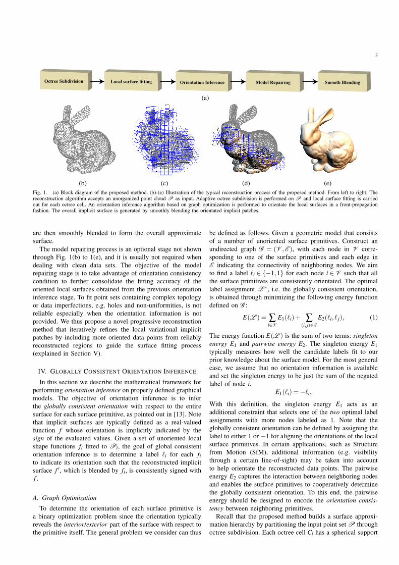
Octree Subdivision Local surface fitting Orientation Inference Model Repairing Smooth Blending

(a)

(b) (c) (d) (e)

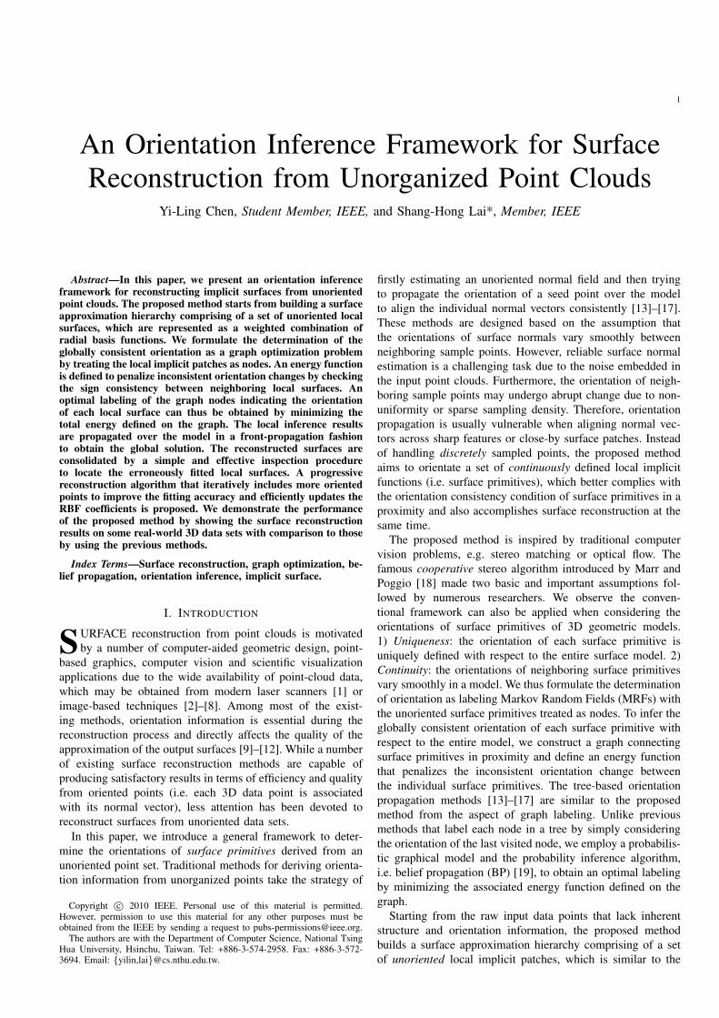
Fig. 1. (a) Block diagram of the proposed method. (b)-(e) Illustration of the typical reconstruction process of the proposed method. From left to right: Thereconstruction algorithm accepts an unorganized point cloud P as input. Adaptive octree subdivision is performed on P and local surface fitting is carriedout for each octree cell. An orientation inference algorithm based on graph optimization is performed to orientate the local surfaces in a front-propagationfashion. The overall implicit surface is generated by smoothly blending the orientated implicit patches.

are then smoothly blended to form the overall approximate

surface.

The model repairing process is an optional stage not shown

through Fig. 1(b) to 1(e), and it is usually not required when

dealing with clean data sets. The objective of the model

repairing stage is to take advantage of orientation consistency

condition to further consolidate the fitting accuracy of the

oriented local surfaces obtained from the previous orientation

inference stage. To fit point sets containing complex topology

or data imperfections, e.g. holes and non-uniformities, is not

reliable especially when the orientation information is not

provided. We thus propose a novel progressive reconstruction

method that iteratively refines the local variational implicit

patches by including more oriented data points from reliably

reconstructed regions to guide the surface fitting process

(explained in Section V).

IV. GLOBALLY CONSISTENT ORIENTATION INFERENCE

In this section we describe the mathematical framework for

performing orientation inference on properly defined graphical

models. The objective of orientation inference is to infer

the globally consistent orientation with respect to the entire

surface for each surface primitive, as pointed out in [13]. Note

that implicit surfaces are typically defined as a real-valued

function f whose orientation is implicitly indicated by the

sign of the evaluated values. Given a set of unoriented local

shape functions fi fitted to Pi, the goal of global consistent

orientation inference is to determine a label `i for each fi

to indicate its orientation such that the reconstructed implicit

surface f ′, which is blended by fi, is consistently signed with

f .

A. Graph Optimization

To determine the orientation of each surface primitive is

a binary optimization problem since the orientation typically

reveals the interior/exterior part of the surface with respect to

the primitive itself. The general problem we consider can thus

be defined as follows. Given a geometric model that consists

of a number of unoriented surface primitives. Construct an

undirected graph G = (V ,E ), with each node in V corre-

sponding to one of the surface primitives and each edge in

E indicating the connectivity of neighboring nodes. We aim

to find a label `i ∈ {−1,1} for each node i ∈ V such that all

the surface primitives are consistently orientated. The optimal

label assignment L ∗, i.e. the globally consistent orientation,

is obtained through minimizing the following energy function

defined on G :

E(L ) = ∑i∈V

E1(`i)+ ∑(i, j)∈E

E2(`i, ` j), (1)

The energy function E(L ) is the sum of two terms: singleton

energy E1 and pairwise energy E2. The singleton energy E1

typically measures how well the candidate labels fit to our

prior knowledge about the surface model. For the most general

case, we assume that no orientation information is available

and set the singleton energy to be just the sum of the negated

label of node i.

E1(`i) =−`i,

With this definition, the singleton energy E1 acts as an

additional constraint that selects one of the two optimal label

assignments with more nodes labeled as 1. Note that the

globally consistent orientation can be defined by assigning the

label to either 1 or −1 for aligning the orientations of the local

surface primitives. In certain applications, such as Structure

from Motion (SfM), additional information (e.g. visibility

through a certain line-of-sight) may be taken into account

to help orientate the reconstructed data points. The pairwise

energy E2 captures the interaction between neighboring nodes

and enables the surface primitives to cooperatively determine

the globally consistent orientation. To this end, the pairwise

energy should be designed to encode the orientation consis-

tency between neighboring primitives.

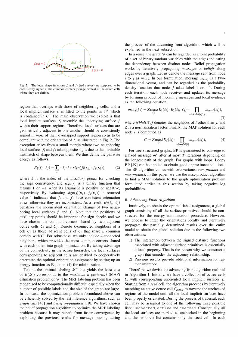
Recall that the proposed method builds a surface approxi-

mation hierarchy by partitioning the input point set P through

octree subdivision. Each octree cell Ci has a spherical support

4

+

–

f(x) = 0

fj (x) = 0

fi (x) = 0

Fig. 2. The local shape functions fi and f j (red curves) are supposed to beconsistently signed at the common corners (orange circles) of the octree cellswhere they are defined.

region that overlaps with those of neighboring cells, and a

local implicit surface fi is fitted to the points in Pi which

is contained in Ci. The main observation we exploit is that

local implicit surfaces fi resemble the underlying surface f

within their support regions. Therefore, local surfaces that are

geometrically adjacent to one another should be consistently

signed in most of their overlapped support region so as to be

compliant with the orientation of f , as illustrated in Fig. 2. The

exception arises from a small margin where two neighboring

local surfaces fi and f j take opposite signs due to the inevitable

mismatch of shape between them. We thus define the pairwise

energy as follows.

E2(`i, ` j) = ∑k

−`i · ` j · sign( fi(xk) · f j(xk)), (2)

where k is the index of the auxiliary points for checking

the sign consistency, and sign(·) is a binary function that

returns 1 or −1 when its argument is positive or negative,

respectively. By evaluating sign( fi(xk) · f j(xk)), a returned

value 1 indicates that fi and f j have consistent orientation

at xk, otherwise they are inconsistent. As a result, E2(`i, ` j)penalizes the inconsistent orientation change of two neigh-

boring local surfaces fi and f j. Note that the positions of

auxiliary points should be important for sign checks and we

have chosen the common corners shared by two adjacent

octree cells Ci and C j. Denote k-connected neighbors of a

cell Ci as those adjacent cells of Ci that share k common

corners with Ci. For robustness, we only include 4-connected

neighbors, which provides the most common corners shared

with each other, into graph optimization. By taking advantage

of the connectivity in the octree hierarchy, the local surfaces

corresponding to adjacent cells are enabled to cooperatively

determine the optimal orientation assignment by setting up an

energy function as Equation (1) for minimization.

To find the optimal labeling L ∗ that yields the least cost

of E(L ) corresponds to the maximum a posteriori (MAP)

estimation problem on G . The MRF labeling problem has been

recognized to be computationally difficult, especially when the

number of possible labels and the size of the graph are large.

In our case, the optimization problem formulated above can

be efficiently solved by the fast inference algorithms, such as

graph cuts [48] and belief propagation [19]. We have chosen

the belief propagation algorithm to optimize the MRF labeling

problem because it may benefit from faster convergence by

exploiting the previous results for message passing during

the process of the advancing-front algorithm, which will be

explained in the next subsection.

In a sense, the graph G can be regarded as a joint probability

of a set of binary random variables with the edges indicating

the dependency between distinct nodes. Belief propagation

works by iteratively propagating messages or beliefs along

edges over a graph. Let us denote the message sent from node

i to j as mi→ j. In our formulation, message mi→ j is a two-

dimensional vector, and can be regarded as the probability

density function that node j takes label 1 or −1. During

each iteration, each node receives and updates its message

by forming product of incoming messages and local evidence

as the following equation:

mi→ j(` j) = Z max` j

(E1(`i) ·E2(`i, ` j) · ∏u∈Nbhd(i)\ j

mu→i(`i)),

(3)

where Nbhd(i)\ j denotes the neighbors of i other than j, and

Z is a normalization factor. Finally, the MAP solution for each

node i is computed as

`∗i = Z max`i

(Ed(`i) · ∏u∈Nbhd(i)

mu→i(`i)), (4)

For tree structured graphs, BP is guaranteed to converge to

a fixed message m∗ after at most T iterations depending on

the longest path of the graph. For graphs with loops, Loopy

BP [49] can be applied to obtain good approximate solutions.

The BP algorithm comes with two variants: sum-product and

max-product. In this paper, we use the max-product algorithm

to find a MAP solution to the graph optimization problem

formulated earlier in this section by taking negative log

probabilities.

B. Advancing-Front Algorithm

Intuitively, to obtain the optimal label assignment, a global

graph consisting of all the surface primitives should be con-

structed for the energy minimization procedure. However,

we choose to infer the orientations locally and iteratively

propagate the partially determined results over the entire

model to obtain the global solution due to the following two

observations:

1) The interaction between the signed distance functions

associated with adjacent surface primitives is essentially

a local property. That is the reason why we construct a

graph that encodes the adjacency relationship.

2) Previous results provide additional information for fur-

ther inference.

Therefore, we devise the advancing-front algorithm outlined

in Algorithm 1. Initially, we have a collection of octree cells

Ci with corresponding unoriented local implicit surfaces fi.

Starting from a seed cell, the algorithm proceeds by iteratively

marching an active octree cell Cactive to traverse the unchecked

regions of the model until all the local implicit surfaces have

been properly orientated. During the process of traversal, each

cell may be assigned to one of the following three possible

lists: unchecked, active and checked. Conceptually, all

the local surfaces are marked as unchecked in the beginning

and the active list contains only the seed cell. In each

5

(a) (b) (c) (d)

(e) (f) (g) (h)

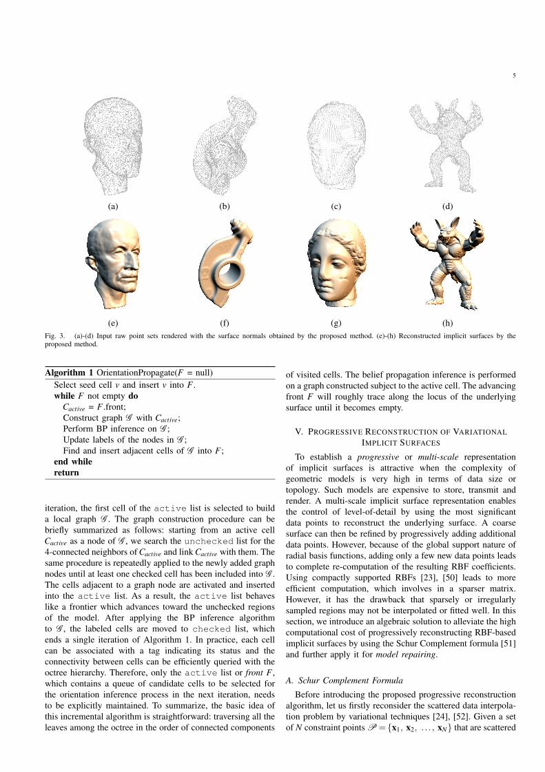
Fig. 3. (a)-(d) Input raw point sets rendered with the surface normals obtained by the proposed method. (e)-(h) Reconstructed implicit surfaces by theproposed method.

Algorithm 1 OrientationPropagate(F = null)

Select seed cell v and insert v into F .

while F not empty do

Cactive = F .front;

Construct graph G with Cactive;

Perform BP inference on G ;

Update labels of the nodes in G ;

Find and insert adjacent cells of G into F ;

end while

return

iteration, the first cell of the active list is selected to build

a local graph G . The graph construction procedure can be

briefly summarized as follows: starting from an active cell

Cactive as a node of G , we search the unchecked list for the

4-connected neighbors of Cactive and link Cactive with them. The

same procedure is repeatedly applied to the newly added graph

nodes until at least one checked cell has been included into G .

The cells adjacent to a graph node are activated and inserted

into the active list. As a result, the active list behaves

like a frontier which advances toward the unchecked regions

of the model. After applying the BP inference algorithm

to G , the labeled cells are moved to checked list, which

ends a single iteration of Algorithm 1. In practice, each cell

can be associated with a tag indicating its status and the

connectivity between cells can be efficiently queried with the

octree hierarchy. Therefore, only the active list or front F ,

which contains a queue of candidate cells to be selected for

the orientation inference process in the next iteration, needs

to be explicitly maintained. To summarize, the basic idea of

this incremental algorithm is straightforward: traversing all the

leaves among the octree in the order of connected components

of visited cells. The belief propagation inference is performed

on a graph constructed subject to the active cell. The advancing

front F will roughly trace along the locus of the underlying

surface until it becomes empty.

V. PROGRESSIVE RECONSTRUCTION OF VARIATIONAL

IMPLICIT SURFACES

To establish a progressive or multi-scale representation

of implicit surfaces is attractive when the complexity of

geometric models is very high in terms of data size or

topology. Such models are expensive to store, transmit and

render. A multi-scale implicit surface representation enables

the control of level-of-detail by using the most significant

data points to reconstruct the underlying surface. A coarse

surface can then be refined by progressively adding additional

data points. However, because of the global support nature of

radial basis functions, adding only a few new data points leads

to complete re-computation of the resulting RBF coefficients.

Using compactly supported RBFs [23], [50] leads to more

efficient computation, which involves in a sparser matrix.

However, it has the drawback that sparsely or irregularly

sampled regions may not be interpolated or fitted well. In this

section, we introduce an algebraic solution to alleviate the high

computational cost of progressively reconstructing RBF-based

implicit surfaces by using the Schur Complement formula [51]

and further apply it for model repairing.

A. Schur Complement Formula

Before introducing the proposed progressive reconstruction

algorithm, let us firstly reconsider the scattered data interpola-

tion problem by variational techniques [24], [52]. Given a set

of N constraint points P = {x1, x2, . . . , xN} that are scattered

6

on or near the unknown surface with the corresponding scalar

height fields h1, h2, . . . , hN , find f that satisfies the inter-

polation conditions: f (xi) = hi, i = 1, 2, . . . , N. Expressing

the interpolant function f as a weighted combination of RBFs

in Equation (5) leads to the smoothest function among all

possible solution functions with minimum aggregate curvature:

f (x) =N

∑j=1

w jφ(x−x j)+ p(x), (5)

where x j = (x j, y j, z j) are the locations of the constraints,

w j are the weights, and p(x) is a first-degree polynomial

accounting for the linear and constant term of f . There

is a rich variety of radial basis functions suggested in the

literature. For 3D interpolation, we adopt the pseudo-cubic

basis function φ(r) = r3, as used in [24], [52]. Solving for

the unknowns, w1, w2, . . . , wN , and the coefficients of p(x),in the interpolation function f leads to solving the following

linear system:

(

A P

PT O

)(

w

λ

)

=

(

h

0

)

, (6)

where Ai j = φ(‖xi − x j‖). The polynomial part of the in-

terpolation function f in Eq. (5) has the form of p(x) =λ0 + λ1x+ λ2y+ λ3z, and thus P is the matrix with the i-th

row being (1,xi,yi,zi). Note that the sub-matrix A is positive-

definite and the solution to Eq. (6) can be easily solved

by direct methods, such as LU decomposition or singular

value decomposition (SVD). Typically, the scalar values h

corresponding to the data points where the implicit surface

passes through are set to zero and some off-surface constraints

inside or outside the surface are created by extending the on-

surface constraints along the directions of surface normals for

a certain distance [24]. It is worth noting that initially we

cannot obtain correctly orientated local surfaces because the

off-surface constraints required to determine the orientation

cannot be explicitly specified in absence of real surface

normals. Orientation inference is thus applied to resolve the

orientations of the local surfaces.

To achieve progressive reconstruction, additional constraint

points are repeatedly appended to the linear system of (6)

and the corresponding RBF coefficients need to be updated.

Since the linear system is getting larger, directly applying

LU decomposition or SVD requires O(N3) computational

complexity to re-compute the RBF coefficients, which is quite

computationally expensive especially when N is large. In this

paper, we propose an algebraic approach to alleviate the cost

of iteratively updating globally supported radial weights by

using the Schur complement formula [51]. Schur complement

formula gives the closed-form expression for the inverse of a

partitioned matrix. Firstly, we rearrange the linear system in

Equation (6) as below:

(

O PT

P A

)(

λw

)

=

(

0

h

)

, (7)

During the process of progressive reconstruction, the matrix of

our progressive reconstruction problem can thus be expressed

by the following 2×2 partitioned matrix:

fi (x)

fj1 (x)fj2 (x)

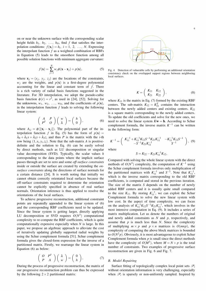
Fig. 4. Detection of vulnerable cells by performing an additional orientationconsistency check on the overlapped support regions between neighboringlocal surfaces.

K =

(

K11 K12

K21 K22

)

, (8)

where K11 is the matrix in Eq. (7) formed by the existing RBF

centers. The sub-matrix K12 = KT21 contains the interaction

between the newly added centers and existing centers. K22

is a square matrix corresponding to the newly added centers.

To update the old coefficients and solve for the new ones, we

need to solve the linear system Kw = h. According to Schur

complement formula, the inverse matrix K−1 can be written

in the following form:

K−1 =

(

K−111 +K−1

11 K12S−1K21K−111 −K−1

11 K12S−1

−S−1K21K−111 S−1

)

, (9)

where

S = K22 −K21K−111 K12,

Compared with solving the whole linear system with the direct

methods of O(N3) complexity, the computation of K−1 using

the Schur complement formula involves only multiplication of

the partitioned matrices with K−111 and S−1. Note that K−1

11 ,

which is the inverse matrix corresponding to the old RBF

coefficients, is computed and stored in the previous iteration.

The size of the matrix S depends on the number of newly

added RBF centers and it is usually quite small compared

to the size K11. By storing K−111 , we can exploit the Schur

Complement formula to solve the new linear system with

low cost. In the aspect of time complexity, we can focus

on the analysis of K−111 K12S−1K21K−1

11 , which involves in the

most intensive computation in Eq. (9). It includes a series of

matrix multiplication. Let us denote the numbers of original

and newly added constraints as N and p, respectively, and

assume that p is much less than N. Since the complexity

of multiplying m × p and p × n matrices is O(mnp), the

complexity of computing the above block matrices is bounded

to O(N2 p). Obviously, it is most advantageous to exploit Schur

Complement formula when p is small since the direct methods

have the complexity of O(M3), where M = N + p is the total

number of constraints. Two examples of progressive surface

reconstruction are given in Fig. 6 and Fig. 7.

B. Model Repairing

Surface fitting of topologically complex local point sets Pi

without orientation information is very challenging, especially

when Pi is sparsely or non-uniformly sampled. Inspired by

7

(a) (b) (c)

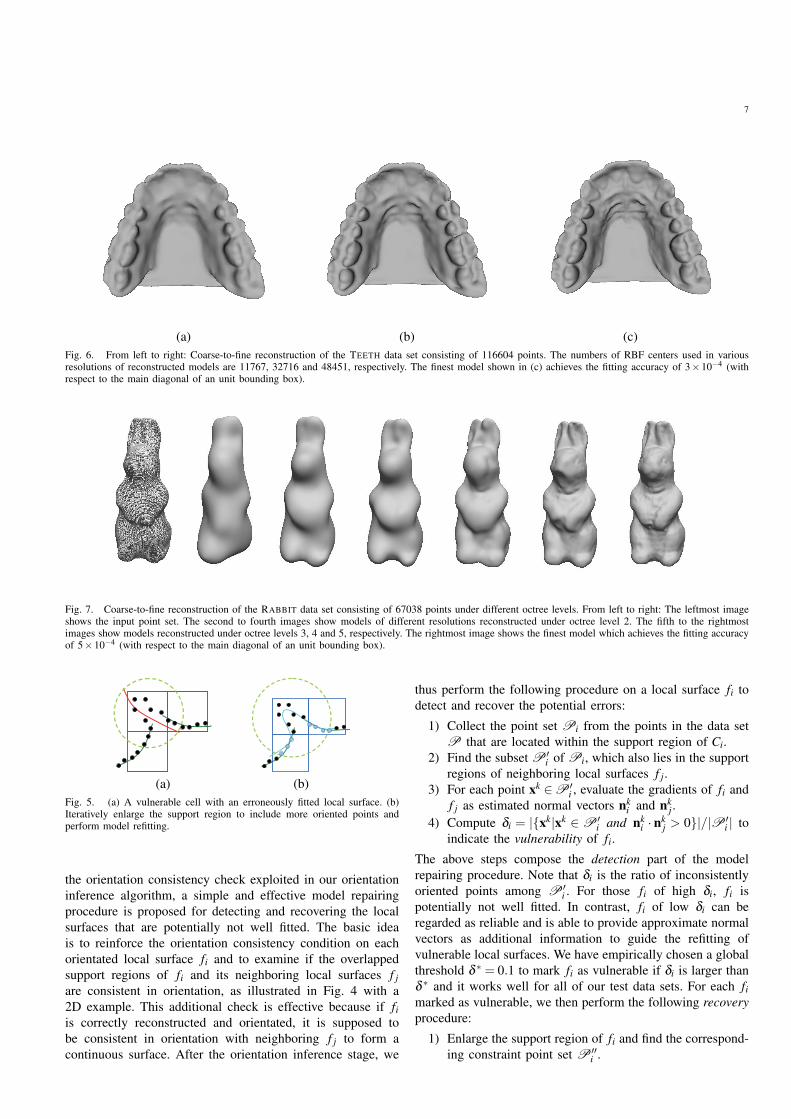
Fig. 6. From left to right: Coarse-to-fine reconstruction of the TEETH data set consisting of 116604 points. The numbers of RBF centers used in variousresolutions of reconstructed models are 11767, 32716 and 48451, respectively. The finest model shown in (c) achieves the fitting accuracy of 3×10−4 (withrespect to the main diagonal of an unit bounding box).

Fig. 7. Coarse-to-fine reconstruction of the RABBIT data set consisting of 67038 points under different octree levels. From left to right: The leftmost imageshows the input point set. The second to fourth images show models of different resolutions reconstructed under octree level 2. The fifth to the rightmostimages show models reconstructed under octree levels 3, 4 and 5, respectively. The rightmost image shows the finest model which achieves the fitting accuracyof 5×10−4 (with respect to the main diagonal of an unit bounding box).

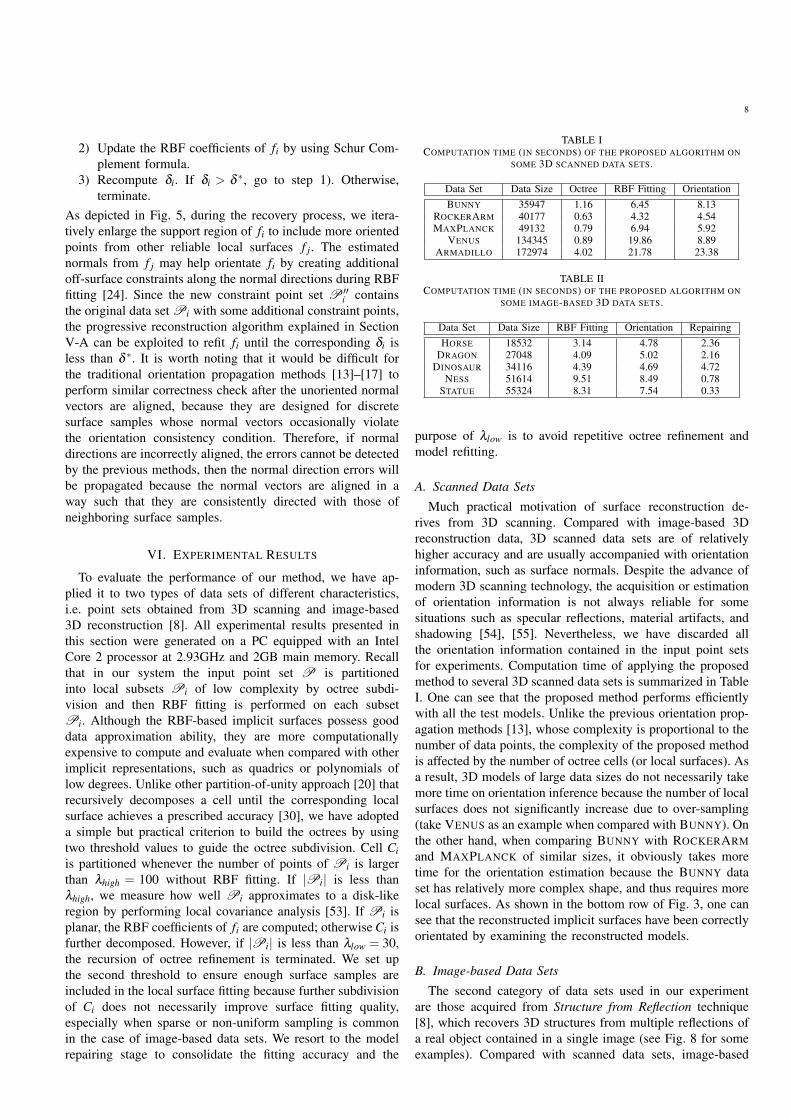
(a) (b)

Fig. 5. (a) A vulnerable cell with an erroneously fitted local surface. (b)Iteratively enlarge the support region to include more oriented points andperform model refitting.

the orientation consistency check exploited in our orientation

inference algorithm, a simple and effective model repairing

procedure is proposed for detecting and recovering the local

surfaces that are potentially not well fitted. The basic idea

is to reinforce the orientation consistency condition on each

orientated local surface fi and to examine if the overlapped

support regions of fi and its neighboring local surfaces f j

are consistent in orientation, as illustrated in Fig. 4 with a

2D example. This additional check is effective because if fi

is correctly reconstructed and orientated, it is supposed to

be consistent in orientation with neighboring f j to form a

continuous surface. After the orientation inference stage, we

thus perform the following procedure on a local surface fi to

detect and recover the potential errors:

1) Collect the point set Pi from the points in the data set

P that are located within the support region of Ci.

2) Find the subset P ′i of Pi, which also lies in the support

regions of neighboring local surfaces f j.

3) For each point xk ∈P ′i , evaluate the gradients of fi and

f j as estimated normal vectors nki and nk

j.

4) Compute δi = |{xk|xk ∈ P ′i and nk

i · nkj > 0}|/|P ′

i | to

indicate the vulnerability of fi.

The above steps compose the detection part of the model

repairing procedure. Note that δi is the ratio of inconsistently

oriented points among P ′i . For those fi of high δi, fi is

potentially not well fitted. In contrast, fi of low δi can be

regarded as reliable and is able to provide approximate normal

vectors as additional information to guide the refitting of

vulnerable local surfaces. We have empirically chosen a global

threshold δ ∗ = 0.1 to mark fi as vulnerable if δi is larger than

δ ∗ and it works well for all of our test data sets. For each fi

marked as vulnerable, we then perform the following recovery

procedure:

1) Enlarge the support region of fi and find the correspond-

ing constraint point set P ′′i .

8

2) Update the RBF coefficients of fi by using Schur Com-

plement formula.

3) Recompute δi. If δi > δ ∗, go to step 1). Otherwise,

terminate.

As depicted in Fig. 5, during the recovery process, we itera-

tively enlarge the support region of fi to include more oriented

points from other reliable local surfaces f j. The estimated

normals from f j may help orientate fi by creating additional

off-surface constraints along the normal directions during RBF

fitting [24]. Since the new constraint point set P ′′i contains

the original data set Pi with some additional constraint points,

the progressive reconstruction algorithm explained in Section

V-A can be exploited to refit fi until the corresponding δi is

less than δ ∗. It is worth noting that it would be difficult for

the traditional orientation propagation methods [13]–[17] to

perform similar correctness check after the unoriented normal

vectors are aligned, because they are designed for discrete

surface samples whose normal vectors occasionally violate

the orientation consistency condition. Therefore, if normal

directions are incorrectly aligned, the errors cannot be detected

by the previous methods, then the normal direction errors will

be propagated because the normal vectors are aligned in a

way such that they are consistently directed with those of

neighboring surface samples.

VI. EXPERIMENTAL RESULTS

To evaluate the performance of our method, we have ap-

plied it to two types of data sets of different characteristics,

i.e. point sets obtained from 3D scanning and image-based

3D reconstruction [8]. All experimental results presented in

this section were generated on a PC equipped with an Intel

Core 2 processor at 2.93GHz and 2GB main memory. Recall

that in our system the input point set P is partitioned

into local subsets Pi of low complexity by octree subdi-

vision and then RBF fitting is performed on each subset

Pi. Although the RBF-based implicit surfaces possess good

data approximation ability, they are more computationally

expensive to compute and evaluate when compared with other

implicit representations, such as quadrics or polynomials of

low degrees. Unlike other partition-of-unity approach [20] that

recursively decomposes a cell until the corresponding local

surface achieves a prescribed accuracy [30], we have adopted

a simple but practical criterion to build the octrees by using

two threshold values to guide the octree subdivision. Cell Ci

is partitioned whenever the number of points of Pi is larger

than λhigh = 100 without RBF fitting. If |Pi| is less than

λhigh, we measure how well Pi approximates to a disk-like

region by performing local covariance analysis [53]. If Pi is

planar, the RBF coefficients of fi are computed; otherwise Ci is

further decomposed. However, if |Pi| is less than λlow = 30,

the recursion of octree refinement is terminated. We set up

the second threshold to ensure enough surface samples are

included in the local surface fitting because further subdivision

of Ci does not necessarily improve surface fitting quality,

especially when sparse or non-uniform sampling is common

in the case of image-based data sets. We resort to the model

repairing stage to consolidate the fitting accuracy and the

TABLE ICOMPUTATION TIME (IN SECONDS) OF THE PROPOSED ALGORITHM ON

SOME 3D SCANNED DATA SETS.

Data Set Data Size Octree RBF Fitting Orientation

BUNNY 35947 1.16 6.45 8.13ROCKERARM 40177 0.63 4.32 4.54MAXPLANCK 49132 0.79 6.94 5.92

VENUS 134345 0.89 19.86 8.89ARMADILLO 172974 4.02 21.78 23.38

TABLE IICOMPUTATION TIME (IN SECONDS) OF THE PROPOSED ALGORITHM ON

SOME IMAGE-BASED 3D DATA SETS.

Data Set Data Size RBF Fitting Orientation Repairing

HORSE 18532 3.14 4.78 2.36DRAGON 27048 4.09 5.02 2.16

DINOSAUR 34116 4.39 4.69 4.72NESS 51614 9.51 8.49 0.78

STATUE 55324 8.31 7.54 0.33

purpose of λlow is to avoid repetitive octree refinement and

model refitting.

A. Scanned Data Sets

Much practical motivation of surface reconstruction de-

rives from 3D scanning. Compared with image-based 3D

reconstruction data, 3D scanned data sets are of relatively

higher accuracy and are usually accompanied with orientation

information, such as surface normals. Despite the advance of

modern 3D scanning technology, the acquisition or estimation

of orientation information is not always reliable for some

situations such as specular reflections, material artifacts, and

shadowing [54], [55]. Nevertheless, we have discarded all

the orientation information contained in the input point sets

for experiments. Computation time of applying the proposed

method to several 3D scanned data sets is summarized in Table

I. One can see that the proposed method performs efficiently

with all the test models. Unlike the previous orientation prop-

agation methods [13], whose complexity is proportional to the

number of data points, the complexity of the proposed method

is affected by the number of octree cells (or local surfaces). As

a result, 3D models of large data sizes do not necessarily take

more time on orientation inference because the number of local

surfaces does not significantly increase due to over-sampling

(take VENUS as an example when compared with BUNNY). On

the other hand, when comparing BUNNY with ROCKERARM

and MAXPLANCK of similar sizes, it obviously takes more

time for the orientation estimation because the BUNNY data

set has relatively more complex shape, and thus requires more

local surfaces. As shown in the bottom row of Fig. 3, one can

see that the reconstructed implicit surfaces have been correctly

orientated by examining the reconstructed models.

B. Image-based Data Sets

The second category of data sets used in our experiment

are those acquired from Structure from Reflection technique

[8], which recovers 3D structures from multiple reflections of

a real object contained in a single image (see Fig. 8 for some

examples). Compared with scanned data sets, image-based

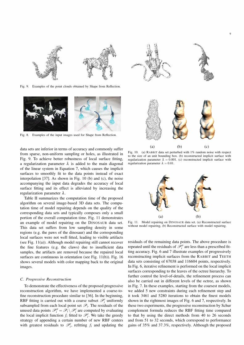
9

Fig. 9. Examples of the point clouds obtained by Shape from Reflection.

Fig. 8. Examples of the input images used for Shape from Reflection.

data sets are inferior in terms of accuracy and commonly suffer

from sparse, non-uniform sampling or holes, as illustrated in

Fig. 9. To achieve better robustness of local surface fitting,

a regularization parameter λ is added to the main diagonal

of the linear system in Equation 7, which causes the implicit

surfaces to smoothly fit to the data points instead of exact

interpolation [37]. As shown in Fig. 10 (b) and (c), the noise

accompanying the input data degrades the accuracy of local

surface fitting and its effect is alleviated by increasing the

regularization parameter λ .

Table II summarizes the computation time of the proposed

algorithm on several image-based 3D data sets. The compu-

tation time of model repairing depends on the quality of the

corresponding data sets and typically composes only a small

portion of the overall computation time. Fig. 11 demonstrates

an example of model repairing on the DINOSAUR data set.

This data set suffers from low sampling density in some

regions (e.g. the paws of the dinosaur) and the corresponding

local surfaces were not well fitted, leading to visible artifacts

(see Fig. 11(a)). Although model repairing still cannot recover

the fine features (e.g. the claws) due to insufficient data

samples, the artifacts are removed because the repaired local

surfaces are continuous in orientation (see Fig. 11(b)). Fig. 16

shows several models with color mapping back to the original

images.

C. Progressive Reconstruction

To demonstrate the effectiveness of the proposed progressive

reconstruction algorithm, we have implemented a coarse-to-

fine reconstruction procedure similar to [36]. In the beginning,

RBF fitting is carried out with a coarse subset P ′i uniformly

subsampled from each local point set Pi. The residuals of the

unused data points P ′′i =Pi \P ′

i are computed by evaluating

the local implicit function fi fitted to P ′i . We take the greedy

strategy of appending a certain number of new RBF centers

with greatest residuals to P ′i , refitting fi and updating the

(a) (b) (c)

Fig. 10. (a) RABBIT data set perturbed with 1% random noise with respectto the size of an unit bounding box. (b) reconstructed implicit surface withregularization parameter λ = 0.001. (c) reconstructed implicit surface withregularization parameter λ = 0.01.

(a) (b)

Fig. 11. Model repairing on DINOSAUR data set. (a) Reconstructed surfacewithout model repairing, (b) Reconstructed surface with model repairing.

residuals of the remaining data points. The above procedure is

repeated until the residuals of P ′′i are less than a prescribed fit-

ting accuracy. Fig. 6 and 7 illustrate examples of progressively

reconstructing implicit surfaces from the RABBIT and TEETH

data sets consisting of 67038 and 116604 points, respectively.

In Fig. 6, iterative refinement is performed on the local implicit

surfaces corresponding to the leaves of the octree hierarchy. To

further control the level-of-details, the refinement process can

also be carried out in different levels of the octree, as shown

in Fig. 7. In these examples, starting from the coarsest models,

we added 5 new constraints during each refinement step and

it took 3461 and 5280 iterations to obtain the finest models

shown in the rightmost images of Fig. 6 and 7, respectively. In

these two experiments, the progressive reconstruction by Schur

complement formula reduces the RBF fitting time compared

to that by using the direct methods from 40 to 26 seconds

and from 51 to 32 seconds, which correspond to performance

gains of 35% and 37.3%, respectively. Although the proposed

10

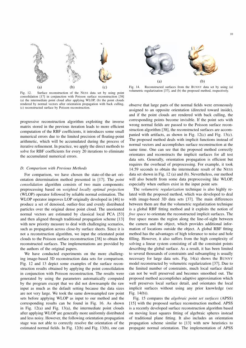
(a) (b) (c)

Fig. 12. Surface reconstruction of the NESS data set by using pointconsolidation [17] in conjunction with Poisson surface reconstruction [38](a) the intermediate point cloud after applying WLOP, (b) the point cloudsrendered by normal vectors after orientation propagation with back culling,(c) reconstructed surface by Poisson reconstruction.

progressive reconstruction algorithm exploiting the inverse

matrix stored in the previous iteration leads to more efficient

computation of the RBF coefficients, it introduces some small

numerical errors due to the limited precision of floating-point

arithmetic, which will be accumulated during the process of

iterative refinement. In practice, we apply the direct methods to

solve for RBF coefficients for every 20 iterations to eliminate

the accumulated numerical errors.

D. Comparison with Previous Methods

For comparison, we have chosen the state-of-the-art ori-

entation determination method presented in [17]. The point

consolidation algorithm consists of two main components:

preprocessing based on weighted locally optimal projection

(WLOP) operator followed by reliable normal estimation. The

WLOP operator improves LOP originally developed in [46] to

produce a set of denoised, outlier-free and evenly distributed

particles over the original dense point cloud. The unoriented

normal vectors are estimated by classical local PCA [53]

and then aligned through traditional propagation scheme [13]

with new priority measure to deal with challenging scenarios,

such as propagation across close-by surface sheets. Since it is

not a reconstruction algorithm, we input the orientated point

clouds to the Poisson surface reconstruction [38] to obtain the

reconstructed surfaces. The implementations are provided by

the authors of the original papers.

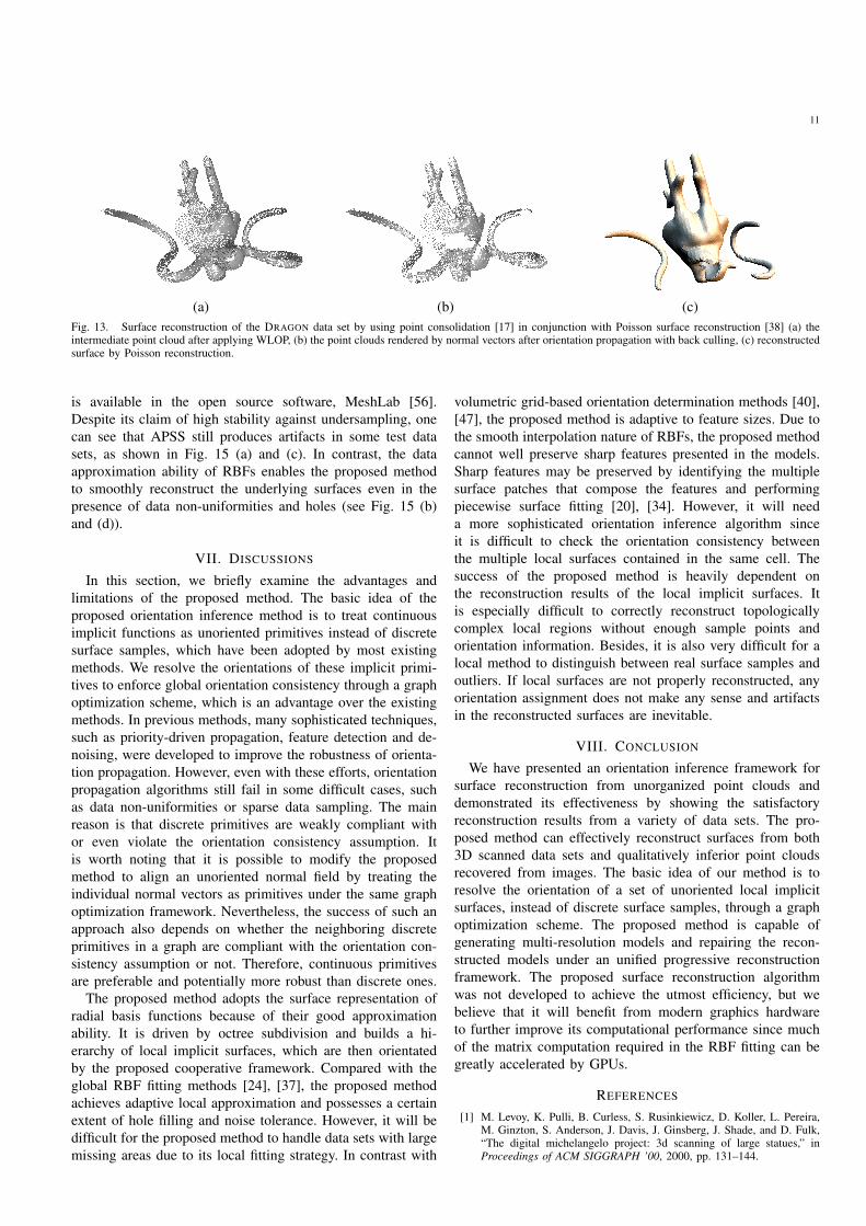
We have conducted experiments on the more challeng-

ing image-based 3D reconstruction data sets for comparison.

Fig. 12 and 13 depict some examples of the surface recon-

struction results obtained by applying the point consolidation

in conjunction with Poisson reconstruction. The results were

generated by using the parameters automatically computed

by the program except that we did not downsample the raw

input as much as the default setting because the data sizes

are not very large. We took the same downsampled raw point

sets before applying WLOP as input to our method and the

corresponding results can be found in Fig. 16. As shown

in Fig. 12(a) and Fig. 13(a), the intermediate point clouds

after applying WLOP are generally more uniformly distributed

and less noisy. However, the following orientation propagation

stage was not able to correctly resolve the orientation of the

estimated normal fields. In Fig. 12(b) and Fig. 13(b), one can

(a) (b)

Fig. 14. Reconstructed surfaces from the BUNNY data set by using (a)volumetric regularization [37], and (b) the proposed method, respectively.

observe that large parts of the normal fields were erroneously

assigned to an opposite orientation (directed toward inside),

and if the point clouds are rendered with back culling, the

corresponding points become invisible. If the point sets with

wrong normal fields are passed to the Poisson surface recon-

struction algorithm [38], the reconstructed surfaces are accom-

panied with artifacts, as shown in Fig. 12(c) and Fig. 13(c).

The proposed method deals with implicit functions instead of

normal vectors and accomplishes surface reconstruction at the

same time. One can see that the proposed method correctly

orientates and reconstructs the implicit surfaces for all test

data sets. Generally, orientation propagation is efficient but

requires the overhead of preprocessing. For example, it took

14.59 seconds to obtain the intermediate result of the NESS

data set shown in Fig. 12 (a) and (b). Nevertheless, our method

will also benefit from some data preprocessing like WLOP,

especially when outliers exist in the input point sets

The volumetric regularization technique is also highly re-

lated with the proposed method, which was developed to deal

with image-based 3D data sets [37]. The main differences

between them are that the volumetric regularization technique

is a global RBF fitting method and it exploits the notion of

free space to orientate the reconstructed implicit surfaces. The

free space means the region along the line-of-sight between

the camera and the object, which provides additional infor-

mation of locations outside the object. A global RBF fitting

method has the advantages of high tolerance to noise and hole

filling. However, it also suffers from the high complexity of

solving a linear system consisting of all the constraint points

describing the global surface. As a result, it has been limited

to several thousands of constraints and subsampling is usually

necessary for large data sets. Fig. 14(a) shows the BUNNY

model reconstructed by volumetric regularization [37]. Due to

the limited number of constraints, much local surface detail

can not be well preserved and becomes smoothed out. The

proposed method accomplishes adaptive approximation which

well preserves local surface detail, and orientates the local

implicit surfaces without using any prior knowledge (see

Fig. 14(b)).

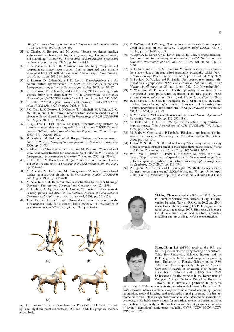
Fig. 15 compares the algebraic point set surfaces (APSS)

[15] with the proposed surface reconstruction method. APSS

is a recently developed surface reconstruction algorithm based

on moving least squares fitting of algebraic spheres instead

of traditional plane fitting. It also includes an orientation

propagation scheme similar to [13] with new heuristics to

propagate normal orientation. The implementation of APSS

11

(a) (b) (c)

Fig. 13. Surface reconstruction of the DRAGON data set by using point consolidation [17] in conjunction with Poisson surface reconstruction [38] (a) theintermediate point cloud after applying WLOP, (b) the point clouds rendered by normal vectors after orientation propagation with back culling, (c) reconstructedsurface by Poisson reconstruction.

is available in the open source software, MeshLab [56].

Despite its claim of high stability against undersampling, one

can see that APSS still produces artifacts in some test data

sets, as shown in Fig. 15 (a) and (c). In contrast, the data

approximation ability of RBFs enables the proposed method

to smoothly reconstruct the underlying surfaces even in the

presence of data non-uniformities and holes (see Fig. 15 (b)

and (d)).

VII. DISCUSSIONS

In this section, we briefly examine the advantages and

limitations of the proposed method. The basic idea of the

proposed orientation inference method is to treat continuous

implicit functions as unoriented primitives instead of discrete

surface samples, which have been adopted by most existing

methods. We resolve the orientations of these implicit primi-

tives to enforce global orientation consistency through a graph

optimization scheme, which is an advantage over the existing

methods. In previous methods, many sophisticated techniques,

such as priority-driven propagation, feature detection and de-

noising, were developed to improve the robustness of orienta-

tion propagation. However, even with these efforts, orientation

propagation algorithms still fail in some difficult cases, such

as data non-uniformities or sparse data sampling. The main

reason is that discrete primitives are weakly compliant with

or even violate the orientation consistency assumption. It

is worth noting that it is possible to modify the proposed

method to align an unoriented normal field by treating the

individual normal vectors as primitives under the same graph

optimization framework. Nevertheless, the success of such an

approach also depends on whether the neighboring discrete

primitives in a graph are compliant with the orientation con-

sistency assumption or not. Therefore, continuous primitives

are preferable and potentially more robust than discrete ones.

The proposed method adopts the surface representation of

radial basis functions because of their good approximation

ability. It is driven by octree subdivision and builds a hi-

erarchy of local implicit surfaces, which are then orientated

by the proposed cooperative framework. Compared with the

global RBF fitting methods [24], [37], the proposed method

achieves adaptive local approximation and possesses a certain

extent of hole filling and noise tolerance. However, it will be

difficult for the proposed method to handle data sets with large

missing areas due to its local fitting strategy. In contrast with

volumetric grid-based orientation determination methods [40],

[47], the proposed method is adaptive to feature sizes. Due to

the smooth interpolation nature of RBFs, the proposed method

cannot well preserve sharp features presented in the models.

Sharp features may be preserved by identifying the multiple

surface patches that compose the features and performing

piecewise surface fitting [20], [34]. However, it will need

a more sophisticated orientation inference algorithm since

it is difficult to check the orientation consistency between

the multiple local surfaces contained in the same cell. The

success of the proposed method is heavily dependent on

the reconstruction results of the local implicit surfaces. It

is especially difficult to correctly reconstruct topologically

complex local regions without enough sample points and

orientation information. Besides, it is also very difficult for a

local method to distinguish between real surface samples and

outliers. If local surfaces are not properly reconstructed, any

orientation assignment does not make any sense and artifacts

in the reconstructed surfaces are inevitable.

VIII. CONCLUSION

We have presented an orientation inference framework for

surface reconstruction from unorganized point clouds and

demonstrated its effectiveness by showing the satisfactory

reconstruction results from a variety of data sets. The pro-

posed method can effectively reconstruct surfaces from both

3D scanned data sets and qualitatively inferior point clouds

recovered from images. The basic idea of our method is to

resolve the orientation of a set of unoriented local implicit

surfaces, instead of discrete surface samples, through a graph

optimization scheme. The proposed method is capable of

generating multi-resolution models and repairing the recon-

structed models under an unified progressive reconstruction

framework. The proposed surface reconstruction algorithm

was not developed to achieve the utmost efficiency, but we

believe that it will benefit from modern graphics hardware

to further improve its computational performance since much

of the matrix computation required in the RBF fitting can be

greatly accelerated by GPUs.

REFERENCES

[1] M. Levoy, K. Pulli, B. Curless, S. Rusinkiewicz, D. Koller, L. Pereira,M. Ginzton, S. Anderson, J. Davis, J. Ginsberg, J. Shade, and D. Fulk,“The digital michelangelo project: 3d scanning of large statues,” inProceedings of ACM SIGGRAPH ’00, 2000, pp. 131–144.

12

(a) (b) (c) (d)

(e) (f) (g) (h)

Fig. 16. (a)-(d): Reconstructed implicit surfaces by applying the proposed method with color mapping. to the image-based 3D reconstructed data sets. (e)-(f):Reconstructed surface models rendered with texture mapping.

[2] A. Robles-Kelly and E. R. Hancock, “A graph-spectral approach toshape-from-shading,” IEEE Transactions on Image Processing, vol. 13,no. 7, pp. 912–926, July 2004.

[3] O. Faugeras and R. Keriven, “Variational principles, surface evolution,pdes, level set methods, and the stereo problem,” IEEE Transactions on

Image Processing, vol. 7, no. 3, pp. 336–344, March 1998.

[4] W. L. Hwang, C.-S. Lu, and P.-C. Chung, “Shape from texture: Es-timation of planar surface orientation through the ridge surfaces ofcontinuous wavelet transform,” IEEE Transactions on Image Processing,vol. 7, no. 5, pp. 773–780, May 1998.

[5] G. Atkinson and E. R. Hancock, “Recovery of surface orientation fromdiffuse polarization,” IEEE Transactions on Image Processing, vol. 15,no. 6, pp. 1653–1664, June 2006.

[6] D. Shin and T. Tjahjadi, “Local hull-based surface construction of volu-metric data from silhouettes,” IEEE Transactions on Image Processing,vol. 17, no. 8, pp. 1251–1260, August 2008.

[7] B. D. Rigling and R. L. Moses, “Three-dimensional surface recon-struction from multistatic sar images,” IEEE Transactions on Image

Processing, vol. 14, no. 8, pp. 1159–1171, August 2005.

[8] P.-H. Huang and S.-H. Lai, “Contour-based structure from reflection,”in Proceedings of IEEE Conference on Computer Vision and Pattern

Recognition (CVPR’06), 2006, pp. 379–386.

[9] M. Alexa, J. Behr, D. Cohen-Or, S. Fleishman, D. Levin, and C. T.Silva, “Point set surfaces,” in Proceedings of IEEE Visualization ’01,October 2001, pp. 21–28.

[10] N. Amenta and Y. J. Kil, “Defining point-set surfaces,” ACM Transac-

tions on Graphics (Proceedings of ACM SIGGRAPH ’04), vol. 23, no. 3,pp. 264–270, 2004.

[11] J.-D. Boissonnat and F. Cazals, “Smooth surface reconstruction vianatural neighbour interpolation of distance functions,” in Proceedings

of annual symposium on Computational geometry, 2000, pp. 223–232.

[12] T. K. Dey and J. Sun, “An adaptive mls surface for reconstruction withguarantees,” in SGP’05: Proceedings of Eurographics Symposium on

Geometry processing, 2005, p. 43.

[13] H. Hoppe, T. DeRose, T. Duchamp, J. McDonald, and W. Stuetzle,“Surface reconstruction from unorganized points,” in Proceedings of

ACM SIGGRAPH ’92, July 1992, pp. 71–78.

[14] H. Xie, J. Wang, J. Hua, H. Qin, and A. Kaufman, “Piecewise c1continuous surface reconstruction of noisy point clouds via local implicitquadric regression,” in Proceedings of IEEE Visualization ’03, 2003, pp.91–98.

[15] G. Guennebaud and M. Gross, “Algebraic point set surfaces,” ACM

Transactions on Graphics (Proceedings of ACM SIGGRAPH ’07),vol. 26, no. 3, pp. 23:1–23:8, 2007.

[16] M. Pauly, R. Keiser, L. Kobbelt, and M. Gross, “Shape modeling withpoint-sampled geometry,” ACM Transactions on Graphics (Proceedings

of ACM SIGGRAPH ’03), vol. 22, no. 3, pp. 641–650, 2003.

[17] H. Huang, D. Li, H. Zhang, U. Ascher, and D. Cohen-Or, “Consol-idation of unorganized point clouds for surface reconstruction,” ACM

Transactions on Graphics (Proceedings of ACM SIGGRAPH Asia ’09),vol. 28, no. 5, pp. 176:1–176:7, 2009.

[18] D. Marr and T. Poggio, “Cooperative computation of stereo disparity,”Science, vol. 194, no. 4262, pp. 283–287, October 1976.

[19] J. Pearl, Probabilistic Reasoning in Intelligent Systems: Networks of

Plausible Inference. San Mateo, California: Morgan Kaufmann, 1988.

[20] Y. Ohtake, A. Belyaev, M. Alexa, G. Turk, and H.-P. Seidel, “Multi-level partition of unity implicits,” in Proc. of ACM SIGGRAPH ’03,July 2003, pp. 463–470.

[21] I. Tobor, P. Reuter, and C. Schlick, “Multi-scale reconstruction ofimplicit surfaces with attributes from large unorganized point sets,” inProceedings of Shape Modeling International ’04, 2004, pp. 19–30.

[22] J. P. Gois, V. Polizelli-Junior, T. Etiene, E. Tejada, A. Castelo, L. G.Nonato, and T. Ertl, “Twofold adaptive partition of unity implicits,” The

Visual Computer, vol. 24, no. 12, pp. 1013–1023, 2008.

[23] Y. Ohtake, A. G. Belyaev, and H.-P. Seidel, “A multi-scale approachto 3d scattered data interpolation with compactly supported basis func-tions,” in Shape Modeling International ’03, May 2003, pp. 153–161.

[24] G. Turk and J. F. O’Brien, “Modelling with implicit surfaces thatinterpolate,” ACM Transactions on Graphics, vol. 21, no. 4, pp. 855–873, October 2002.

[25] H. Edelsbrunner and E. P. Mucke, “Three-dimensional alpha shapes,”ACM Transactions on Graphics, vol. 13, no. 1, pp. 43–72, 1994.

[26] N. Amenta, S. Choi, and R. K. Kolluri, “The power crust,” in Proceed-

ings of ACM symposium on Solid modeling and applications, 2001, pp.249–266.

[27] T. K. Dey and J. Giesen, “Detecting undersampling in surface recon-struction,” in SCG ’01: Proceedings of Symposium on Computational

geometry, 2001, pp. 257–263.

[28] T. K. Dey, J. Giesen, and J. Hudson, “Delaunay based shape reconstruc-tion from large data,” in Proceedings of IEEE Symposium on Parallel

and Large Data Visualization, 2001, pp. 19–27.

[29] F. Cazals and J. Giesen, “Delaunay triangulation based surface re-construction,” in Effective Computational Geometry for Curves and

Surfaces. Springer, 2006.

[30] G. Taubin, “An improved algorithm for algebraic curve and surface

13

fitting,” in Proceedings of International Conference on Computer Vision

(ICCV’93), May 1993, pp. 658–665.

[31] Y. Ohtake, A. Belyaev, and M. Alexa, “Sparse low-degree implicitsurfaces with applications to high quality rendering, feature extraction,and smoothing,” in SGP’05: Proceedings of Eurographics Symposium

on Geometry processing, 2005, pp. 149:1–149:8.

[32] H.-K. Zhao, S. Osher, B. Merriman, and M. Kang, “Implicit andnonparametric shape reconstruction from unorganized data using avariational level set method,” Computer Vision Image Understanding,vol. 80, no. 3, pp. 295–314, 2000.

[33] Y. Lipman, D. Cohen-Or, and D. Levin, “Data-dependent mls forfaithful surface approximation,” in SGP’07: Proceedings of the fifth

Eurographics symposium on Geometry processing, 2007, pp. 59–67.

[34] S. Fleishman, D. Cohen-Or, and C. T. Silva, “Robust moving least-squares fitting with sharp features,” ACM Transactions on Graphics

(Proceedings of ACM SIGGRAPH’05), vol. 24, no. 3, pp. 544–552, 2005.

[35] R. Kolluri, “Provably good moving least squares,” in SIGGRAPH ’05:

ACM SIGGRAPH 2005 Courses, 2005, p. 213.

[36] J. C. Carr, R. K. Beatson, J. B. Cherrie, T. J. Mitchell, W. R. Fright, B. C.McCallum, and T. R. Evans, “Reconstruction and representation of 3dobjects with radial basis functions,” in Proceedings of ACM SIGGRAPH

’01, August 2001, pp. 67–76.

[37] H. Q. Dinh, G. Turk, and G. Slabaugh, “Reconstructing surfaces byvolumetric regularization using radial basis functions,” IEEE Transac-

tions on Pattern Analysis and Machine Intelligence, vol. 24, no. 10, pp.1358–1371, October 2002.

[38] M. Kazhdan, M. Bolitho, and H. Hoppe, “Poisson surface reconstruc-tion,” in Proc. of Eurographics Symposium on Geometry Processing,2006, pp. 61–70.

[39] P. Alliez, D. Cohen-Steiner, Y. Tong, and M. Desbrun, “Voronoi-basedvariational reconstruction for unoriented point sets,” in Proceedings of

Eurographics Symposium on Geometry Processing, 2007, pp. 39–48.

[40] H. Xie, K. T. McDonnel, and H. Qin, “Surface reconstruction of noisyand defective data sets,” in Proceedings of IEEE Visualization ’04, 2004,pp. 259–266.

[41] N. Amenta, M. Bern, and M. Kamvysselis, “A new voronoi-basedsurface reconstruction algorithm,” in Proceedings of ACM SIGGRAPH

’98, August 1998, pp. 415–420.

[42] N. Amenta and M. Bern, “Surface reconstruction by voronoi filtering,”Geometry: Discrete and Computational Geometry, vol. 22, 1999.

[43] N. J. Mitra, A. Nguyen, and L. Guibas, “Estimating surface normalsin noisy point cloud data,” in International Journal of Computational

Geometry and Applications, vol. 14, no. 4–5, 2004, pp. 261–276.

[44] T. K. Dey, G. Li, and J. Sun, “Normal estimation for point clouds:a comparison study for a voronoi based method,” in Proceedings of

Symposium on Point-Based Graphics, 2005, pp. 39–46.

(a) (b)

(c) (d)

Fig. 15. Reconstructed surfaces from the DRAGON and HORSE data setsby (a)(c) algebraic point set surfaces [15], and (b)(d) the proposed method,respectively.

[45] D. OuYang and H.-Y. Feng, “On the normal vector estimation for pointcloud data from smooth surfaces,” Computer-Aided Design, vol. 37,no. 10, pp. 1071–1079, 2005.

[46] Y. Lipman, D. Cohen-Or, D. Levin, and H. Tal-Ezer, “Parameterization-free projection for geometry reconstruction,” ACM Transactions on

Graphics (Proceedings of ACM SIGGRAPH ’07), vol. 26, no. 3, p. 22,2007.

[47] A. C. Jalba and J. B. T. M. Roerdink, “Efficient surface reconstructionfrom noisy data using regularized membrane potentials,” IEEE Trans-

actions on Image Processing, vol. 18, no. 5, pp. 1119–1134, May 2009.[48] Y. Boykov, O. Veksler, and R. Zabih, “Fast approximate energy min-

imization via graph cuts,” IEEE Transactions on Pattern Analysis and

Machine Intelligence, vol. 23, no. 11, pp. 1222–1239, November 2001.[49] Y. Weiss and W. T. Freeman, “On the optimality of solutions of the

max-product belief propagation algorithm in arbitrary graphs,” IEEE

Transactions on Information Theory, vol. 47, no. 2, pp. 723–735, 2001.[50] B. S. Morse, T. S. Yoo, P. Rheingans, D. T. Chen, and K. R. Subra-

manian, “Interpolating implicit surfaces from scattered data using com-pactly supported radial basis functions,” in Shape Modeling International

’01, May 2001, pp. 89–98.[51] D. V. Ouellette, “Schur complements and statistics,” Linear Algebra and

its Applications, vol. 36, pp. 187–295, 1981.[52] G. Turk and J. F. O’Brien, “Shape transformation using variational

implicit surfaces,” in Proceedings of ACM SIGGRAPH ’99, August1999, pp. 335–342.

[53] M. Pauly, M. Gross, and L. P. Kobbelt, “Efficient simplification of point-sampled surfaces,” in Proceedings of IEEE Visualization ’02, October2002, pp. 163–170.

[54] J. Sun, M. Smith, L. Smith, and A. Farooq, “Examining the uncertaintyof the recovered surface normal in three light photometric stereo,” Image

and Vision Computing, vol. 25, no. 7, pp. 1073–1079, 2007.[55] W.-C. Ma, T. Hawkins, P. Peers, C.-F. Chabert, M. Weiss, and P. De-

bevec, “Rapid acquisition of specular and diffuse normal maps frompolarized spherical gradient illumination,” in Eurographics Symposium

on Rendering 2007, 2007, pp. 183–194.[56] P. Cignoni, M. Corsini, and G. Ranzuglia, “Meshlab: an open-source

3d mesh processing system,” ERCIM News, no. 73, pp. 45–46, April2008. [Online]. Available: http://vcg.isti.cnr.it/Publications/2008/CCR08

Yi-Ling Chen received the B.S. and M.S. degreesin Computer Science from National Tsing Hua Uni-versity, Hsinchu, Taiwan, R.O.C. in 2002 and 2004,respectively. He is pursuing his Ph.D degree in thesame department since 2005. His research interestsinclude computer vision and graphics, geometricmodeling and processing, surface reconstruction.

Shang-Hong Lai (M’95-) received the B.S. andM.S. degrees in electrical engineering from NationalTsing Hua University, Hsinchu, Taiwan, and thePh.D. degree in electrical and computer engineeringfrom University of Florida, Gainesville, in 1986,1988 and 1995, respectively. He joined SiemensCorporate Research in Princeton, New Jersey, asa member of technical staff in 1995. Since 1999,he became a faculty member in the Department ofComputer Science, National Tsing Hua University,Taiwan. He is currently a professor in the same

department. In 2004, he was a visiting scholar with Princeton University. Dr.Lai’s research interests include computer vision, visual computing, patternrecognition, medical imaging, and multimedia signal processing. He has au-thored more than 150 papers published in the related international journals andconferences. He holds many patents for inventions related to computer visionand medical image analysis. He has been a member of program committeeof several international conferences, including CVPR, ICCV, ECCV, ACCV,ICPR and ICME.