An investigation of intersection traffic state classification using vehicle delay information

Sajad Shiravi, PhD Candidate, University of Waterloo Liping Fu, Professor, University of Waterloo

Paper prepared for presentation at the Big Data Applications for Travel Demand Management Session

Of the 2016 Conference of the Transportation Association of Canada Toronto, ON

Abstract

The rapid technology evolution in the past decade promises new methods of road traffic data collection with enhanced quantity and quality. These advances are coupled with the development of cost effective platforms to establish sensor and controller networks providing the opportunity to integrate heterogeneous traffic data sources. With these advances and the prospect of big traffic data, it has become possible to measure traffic information such as vehicle travel time/delay information directly. This paper investigates the possibility of using the distribution of vehicle delay information, obtained from historical traffic data, at signalized intersections to classify the traffic state. This classification can be used as a reliable estimate of the traffic demand with various applications such as demand management or traffic signal optimization. The similarities between the delay distributions observed and the traffic state distributions are quantified and compared using several divergence tests including the Chi-Square test, Hellinger distance and the Jensen-Shanon test through simulation. A systematic evaluation under a variety of traffic and driving behavior variable ranges is conducted and the results clearly show that vehicle delay distribution can be used as an effective feature to correctly classify the traffic state using only a few days of historical travel time information and obtain a reliable estimate of the degree of saturation of lane groups at signalized intersections.

Background

Traffic congestion is a widespread problem in major cities around the globe. In a recent report by TomTom, a major provider and collector of traffic travel time data, it is revealed that an average commuter in major cities in Canada such as Toronto, Vancouver, and Montreal experience an average of 84 hours of delay annually (TomTom International, 2014). The lost time reported was 77 hours in the 2013 report by the same company. In this report the congestion rates in Vancouver and Toronto are estimated to be 35 and 31 percent respectively, placing them in the top most congested cities in Canada. Congestion rate is a measure of increase in the travel time compared to non-congested conditions. In international congestion rankings the city of Toronto stands only 2 ranks lower than New York City, despite being approximately 7 times less populated. A report by INRIX, the largest collector and provider of traffic data, estimates that drivers in the U.S alone experienced a total amount of roughly 5.5 billion hours of delay in congestion in 2011 (Schrank, et al., 2012). Considering the increasing growth rate of urban population and the prediction of recovery in the global economy it is only expected that the time spent in congestion will continue to increase. Delay is more an immediate effect of congestion which is strongly felt by commuters. Other effects include increase in fuel consumption, pollutant emissions, road and highway maintenance costs and even an increase in risks for collisions (Halkias, et al., 2004). In terms of monetary value it is estimated that delay and congestion is costing the average US household $1,700 per year (INRIX Center of Economics and Business Research, 2014). The growing demand for transportation can be met by either expanding the infrastructure, reducing the demand, or to make more efficient use of current infrastructure. However, increasing the capacity through the expansion of the transportation infrastructure is costly and constrained by space limitation. Therefore, researchers have sought to develop strategies to make more efficient use of the already available infrastructure. For example, one study shows that imperfect signal timing accounts for almost 300 million vehicle-hours of delay on major roads in North America (National Transportation Operations Coalition, 2007). Among the potential solutions, adaptive signal control systems are effective strategies in enhancing the traffic network efficiency.

Literature Review

Advances in traffic surveillance technology have provided the opportunity to observe traffic variables other than the traditional flow information. Technologies such as wireless BT/Wi-Fi detectors or crowdsourced information obtained from online map apps or navigation applications directly measure performance indicators such as travel time information. Literature related to the direct usage of performance measures, such as the average travel time, for traffic control and management purposes is very limited. The main reason for this is that these technologies are rather new and that the market-penetration of the data collected has been too low until recently to obtain a reliable estimate of the average traffic conditions. One limitation associated with using travel time information is that only a fraction of the vehicles traversing an intersection are observable. In this section a summary will be provided of the studies which have employed travel time information for traffic signal control purposes.

Massart and Koshi (1995) developed one of the earliest control strategies using solely travel time information obtained from roadside traffic beacons. The travel time information is obtained from a fraction of vehicles equipped with the communication technology. The method is proposed for undersaturated and near saturated conditions. The main idea of the research is to estimate the traffic

characteristics from delay information by developing a phase delay profile. A phase delay profile is a profile of the decreasing pattern of delays within a cycle. Based on this information the time duration of the queue is estimated along with an estimation of the saturation flow rate by assuming the exact market penetration rate of the equipped vehicles. Based on the calculated traffic characteristics the signal cycle length and green split are optimized through a routine signal optimization procedure using traffic flow information. The algorithm is tested on a two phase hypothetical intersection in a simulated environment. The implemented algorithm was shown to yield reduced delays compared to fixed time control strategy without mentioning whether the fixed time control was optimized or not. The main limitations of the algorithm is its unreasonable data availability assumptions and limitations to isolated intersections.

Asano (2003) proposed an adaptive signal control system using real-time delay measurements called CARREN. The main data source of the CARREN system is the Automatic Vehicle Identification (AVI) detectors. AVI observes and matches vehicle license plates upon entering exiting the roadway therefore measuring the vehicle’s travel time in the link. As illustrated in Figure 2.5 the cumulative arrival and departure curve are drawn using the travel time information and the total delay which is equivalent to the area under the arrival-departure curve. CARREN optimizes the signal cycle, green split and offset with the objective of minimizing the total delay time. The proposed system requires extensive equipment installment that may not be practical in real applications. With advances in sensor and communication technologies this algorithm may be applicable to new data sources but still requires high resolution data such as that of the connected vehicle technology.

Liu (Liu, et al., 2001) proposed an online traffic signal control system which functions using a real-time delay estimation algorithm. Delay information is obtained through vehicle re-identification technology. In this study a delay projection model is proposed based on historical data. The allocated cycle time is distributed proportionally to the E-W and N-S approaches according to their projected delay. This signal control strategy is tested on an isolated intersection through simulation and proves to decrease delays compared to a fixed time control. The main drawback of this research is its limitation to isolated intersections. In addition, due to lack of historical data a delay projection model has not been developed and the delay in the previous cycle is assumed to be the same for the next cycle.

In another study (MAUTC, 2011) a real-time signal control system is presented which takes use of cumulative travel time (CTT) information assumed to be obtained from equipped connected vehicles. The main idea is to monitor the cumulative travel time of the vehicles for each movement at an intersection and terminate the phase when the CTT of the movements given green are no longer the highest value. The green time will then be assigned to the phases with the highest CTT value. However, under imperfect market penetration rates (market penetration rates of less than 100%) the CTT estimates are inaccurate therefore this study takes use of Kalman Filter to improve the estimations. A major assumption in this research is that at any time a reasonable estimate of the total count of vehicles in each approach of the intersection is available.

The main aim of this study is to develop a method that uses historical travel time information (from several days at the same hour of the day) of a portion of vehicles at signalized intersections to estimate the traffic conditions and then to optimize the traffic signal timing parameters.

Vehicle delay distributions

The delay that vehicles experience at signalized intersections depends on a variety of variables as summarized in Figure 1, the main variables are the signal control parameters, lane configuration and geometric layout, vehicle arrivals and the saturation flow rate. Many traffic and driving behavior factors can potentially affect the saturation flow rate as detailed in Figure… Therefore, different combinations of these factors can generate the same saturation flow rate. The main idea in this research is that firstly the distributions of vehicle delays differ for different degrees of saturation under similar capacity conditions. Secondly, that for a specific degree of saturation the distributions of delays heavily depend on the underlying saturation flow rate considering that a combination of a variety of variables can affect it. This study evaluates the usage of vehicle delay distributions to classify the traffic conditions by generating a series of prototype base-scenarios and to estimate the degree of saturation of a given traffic scenario by finding the closest match to the generated porotypes.

Figure 1: Factors that affect the distribution of vehicle delays at signalized intersections

Effective variables

Signal control parameters

Cycle

Effective green

Amber

Arrival process

Consider Poisson with different seeding

(isolated intersection)

Saturation flow rate

Traffic variables

Turning proportions

On-coming traffic

Heavy vehicles

Pedestrians

Near-by bus stops

Behaviour variables

Lane change distance

Gap acceptance

No of observed preceding vehicles

Minimum headway

Desired Acceleration

Standstill distance

Geometric features

Minimum Distance Classification

A minimum distance classifier assigns the input data to a class that minimizes a defined classification metric. In this method the input is compared against prototype classes and is then classified as the closest prototype in a feature space. In this context, the boundary between the classes is considered the mid-point value. Figure 2 provides a diagram of the classification process.

Figure 2: Minimum distance classification process

A statistical distance quantifies the distance between two probability density functions. Pdf similarity measures can be divided into two categories, vector based and probability based. In vector based approaches the overlap between two pdfs is considered as the distance. Probabilistic distances are built upon the likelihood ratio of the two distributions which can be defined as:

In the context of traffic state estimation, the basis for this classification is that the degree of saturation of a lane-group at an intersection can be described by the probability density

Input Data D d(M1,D)

Class M1

Class M2

d(M2,D)

Class Mc

d(Mc,D)

Minimum Selection

Class

...

function of the delays experienced. The delay distributions of the movements are generally skewed to right in undersaturated conditions with most of the delays occurring in the lower ranges. As the degree of saturation increases, the peak section reduces and an increase in the higher delay values is observed. Figure 3 shows the distribution of delays for different degrees of saturation for a given scenario.

Figure 3: Sample delay distributions

Distance Measure

Many distance measures have been developed for pdf comparisons. One source summarizes more than 45 methods Cha (2007). The Hellinger distance is well-known measure for classification problems. Studies have shown that the Hellinger distance is well capable of distinguishing between similar probability density functions with only slight differences. The Hellinger distance is also known for its ability to handle outliers without affecting its performance which is ideal for situations with imperfect models.

The Jensen-Shanon divergence is also a popular measure that is frequently used for pattern recognition and distance metric learning algorithms defined as follows.

Chi Square is also a frequently used test that is used in this research defined as follows:

0

0.25

0 20 40 60 80 100 120 140 160

Pro

po

rtio

n (

%)

Vehicle delay (s)

0.4

0.5

0.6

0.7

0.8

0.9

The ability of these measures in distinguishing between similar distributions is demonstrated as follows. For this purpose it is assumed that the distribution of delays experienced at a signalized intersection can be roughly approximated by a log-normal distribution. The log-normal distribution, as defined in the equation below, contains 2 parameters, mean and standard deviation. In a log-normal distribution the standard deviation controls the shape of the distribution. The figure below shows the changes in the distribution shape as the standard deviation varies from 0.7 to 1.7.

This can be an approximate representative of changes in the distribution of delays at a signalized intersection corresponding to changes in the degree of saturation. By using the general function of the log-normal distribution the aforementioned distances are then calculated by comparing all distributions with a base log-normal distribution with a standard deviation of 1. As can be seen in Figures 5 and 6, all three distance measures are well capable of distinguishing between the probability densities that only slightly vary which is expected for delay distributions in different degrees of saturations at signalized intersections.

Figure 4: Log normal distributions generated, stdev: 0.7-1.7

0

0.2

0.4

0.6

0.8

1

1.2

0 0.5 1 1.5 2 2.5 3 3.5

f(X

)

X

0.7

0.8

0.9

1

1.1

1.2

1.3

1.4

1.5

1.6

1.7

Figure 5: Comparison of Hellinger and Jensen-Shanon distances with varying standard deviation of the lognormal

distribution

Traffic State Classification

Following the minimum distance classification process, the main aim of this study is to classify the traffic state (i.e. degree of saturation) using the distribution of the delays that vehicles experience when passing through the signalized intersection. The classes and the delay

experienced (received) are represented by probability density functions as )(xpids and )(xpr

respectively. The classes ( )(xpds ), which are the degrees of saturations, are developed with

0.05 increments ranging from 0.4 to 1.0 using simulation based on a given scenario configuration. In this method the signal timing parameters are assumed to be available. The probability density function of each class is developed based on 10 hours of simulation and the pdfs of different degrees of saturations are obtained by increasing the volume for each scenario to achieve the desired degree of saturation.

Evaluation

To evaluate the performance of the proposed method, VISSIM 6 a well-known micro simulation software is used. As highlighted in Figure 6 the evaluation contains 3 main steps. The first step was to generate base-scenario histograms for a series of capacity (saturation flow rates) values. This includes generating 6 capacity scenarios ranging from 2250 vph to 1750 vph. For each capacity 6 base scenarios for degrees of saturations ranging from 0.4 to 0.9 are generated with 0.05 increments. This totals to 66 histograms called the base scenario histograms which the incoming data would be compared to.

0

0.2

0.4

0.6

0.8

1

1.2

0 0.5 1 1.5 2 2.5

Dis

tan

ce (

no

rmal

ize

d)

Stdev

Hellinger Distance

Jensen-Shanon

Chi-Square

Figure 6: Flow chart of the evaluation process

In developing the base scenarios the following assumptions were made:

Geometry is known 2 lane approach with one shared right-through lane and another only through lane 70 s cycle length with 37 seconds of EB-WB green time plus 4 seconds of amber and all-

red 20-80 right turn ratio Safety distance: add: 2 and Multi: 3 m Min headway: 3.0m Preceding vehicles obs: 4 Standstill distance: 3m Speed: car: 50 km/h - HV:30km/h Lane change distance: 175m 10 - 1 hours of simulation for each scenario using different seeding for each run

As previously shown in Figure 1, a variety of driving behavior and traffic variables can potentially affect the saturation flow rate and therefore the capacity of a movement at a signalized intersection. The base scenarios in this study are generated based on a specific combination of driver behavior variables but the proposed method is evaluated based on a variety of ranges of traffic and driver behavior parameters. To represent the driving behavior variables, 7 calibrated Vissim driving behavior cases obtained from Park (2003) are used as shown in Table 1.

Classification and Comparison

Follow process flow chart, calculate histogram distances and classify the input data into one of the available degrees of saturations (classes)

Evaluation scenarios

Generate evaluation scenarios systematically changing traffic and driver behavior parameters

Generate histogram for each base scenario

6 capacity scenarios ranging from 2250 vph to 1750 vph

11 degrees of saturation for each base scenario 0.4-0.9 with 0.05 increments

Table 1: Vissim driver behavior calibrated parameters based on Park (2003)

Parameter Case 1 Case 2 Case 3 Case 4 Case 5 Case 6 Case 7 Lane change

distance (m) 200 150 200 150 200 175 175

No. of observed

vehicles 3 2 3 3 4 4 4

Standstill Distance (m)

3.0 3.0 3.0 3.0 3.0 3.0 3.0

Minimum Headway (m) 2.5 2.5 3.0 2.0 3.0 3.5 3.0

To represent changes in traffic conditions a wide range of turning ratios, heavy vehicle percentages, pedestrian volume and vehicle volumes are considered as shown in Table 2 to evaluate the proposed method for each evaluation scenario one random value is chosen for each variable from the ranges brought in the Table. This is accompanied by randomly selecting a behavior case from one of the 7 cases brought in Table 1 For the sake of this evaluation, 50 scenarios are randomly generated using the mentioned method. Each evaluation scenario is simulated for 10 - 1 hour runs with different seedings in each simulation run. 10 hours is used to represent 10 days of historical data of presumably the same hour of the day in similar conditions.

Table 2: Traffic factors and ranges for evaluation

Parameter Range

Heavy vehicle 0-5%

Pedestrian volume 0-200 ped/hour

Turning ratio 5 to 40%

Volume 700-1450 vph

Using the histogram distance measures previously explained, the input data is then compared with the base scenarios and the lowest 2 distance values are obtained. The corresponding degrees of saturation to these values are then recorded as the degree of saturation for the given scenario. If the degrees of saturations differ, a range is reported as the result between the two values. The three distance measures are obtained for each scenario which it is concluded that the Chi-Square method provides the most accurate results. Therefore, the Chi-square test is selected as the distance measure for this evaluation.

Table 3 provides a sample of the results obtained which details the randomly chosen scenarios along with their actual degree of saturation (X real) followed by the degree of saturation obtained through the proposed method in this study (X estimated).

Table 3: Sample evaluation scenarios generated and final results

right turn prop (%)

40 35 30 30 35 35 25 30 30 20 15

ped (ped/h) 200 80 50 100 120 200 100 60 80 160 140

Heavy Vehicle (%)

0 0 2 0 0 5 3 1 4 0 0

Behavior case 3 6 3 6 4 5 5 6- 3-4 safety

5 7 5

Volume (v/h) 1300 950 1000 1050 850 950 850 900 1100 1100 1100

X real 0.9 0.68 0.57 0.61 0.62 0.68 0.7 0.57 0.72 0.62 0.65

X estimated 0.9 0.65-0.7

0.55 0.6-0.65 0.6 0.65-0.7 0.65-0.7

0.5-0.55 0.7-0.75

0.6-0.65

0.6-0.65

right turn prop (%)

40 20 30 20 25 20 10 25 25 30 20

ped (ped/h) 50 20 120 20 160 100 20 80 20 140 20

Heavy Vehicle (%)

4 3 4 3 0 2 0 3 0 0 0

Behavior case 5 7 5 7 with 3-4

safety 4

6- 3-4 safety

6 4 3 5 4

Volume (v/h) 850 105

0 1100 1050 1150 1000 1500 900 850 1000 1100

Xreal 0.59 0.58 0.65 0.64 0.73 0.6 0.71 0.63 0.55 0.69 0.57

Xestimated 0.5 0.55-0.6

0.65-0.7

0.65-0.7 0.7 0.6-0.65 0.65-0.7

0.6-0.65 0.5-0.55

0.65-0.7

0.6

The final evaluation shows that in 45 out of the 50 scenarios the proposed method is capable of accurately identifying the degree of saturation of the considered lane group. In the other 5 cases the proposed method either over estimates or underestimates the degree of saturation by one bin (0.05).

To evaluate the proposed method in terms of its effects on signal optimization and retiming a hypothetical isolated intersection with known traffic conditions and signal timing parameters is considered. The signal timing is already optimized and the proportionate amount of green time is assigned to each phase based on the current traffic conditions. The main idea in this evaluation is to increase the degree of saturation in one or both movements and demonstrate how the proposed method performs in capturing the changes and be used to improve the signal timing efficiency compared to a “do nothing” alternative. It is important to mention that the degree of saturation can change by either increase in volume or decrease in capacity which both situations are evaluated in this study. The data is generated for 5 days with different

random seeding for each day. The proposed method is evaluated using both complete market penetration rate and using a sample of the data.

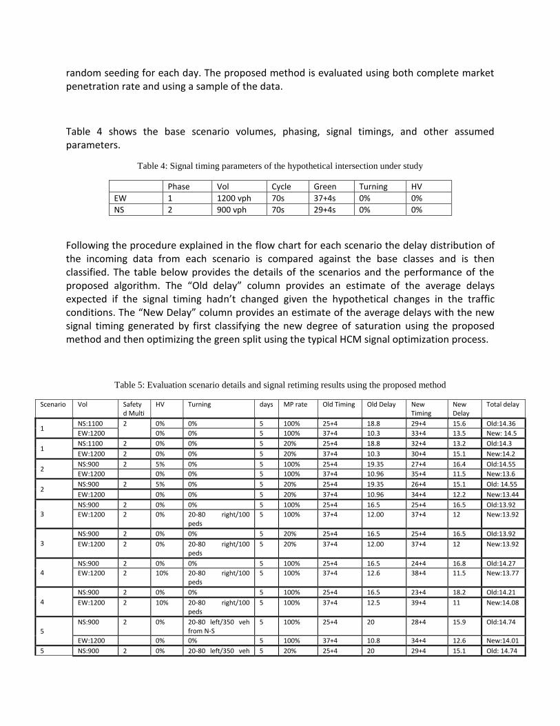
Table 4 shows the base scenario volumes, phasing, signal timings, and other assumed parameters.

Table 4: Signal timing parameters of the hypothetical intersection under study

Phase Vol Cycle Green Turning HV

EW 1 1200 vph 70s 37+4s 0% 0%

NS 2 900 vph 70s 29+4s 0% 0%

Following the procedure explained in the flow chart for each scenario the delay distribution of the incoming data from each scenario is compared against the base classes and is then classified. The table below provides the details of the scenarios and the performance of the proposed algorithm. The “Old delay” column provides an estimate of the average delays expected if the signal timing hadn’t changed given the hypothetical changes in the traffic conditions. The “New Delay” column provides an estimate of the average delays with the new signal timing generated by first classifying the new degree of saturation using the proposed method and then optimizing the green split using the typical HCM signal optimization process.

Table 5: Evaluation scenario details and signal retiming results using the proposed method

Scenario Vol Safety d Multi

HV Turning days MP rate Old Timing Old Delay New Timing

New Delay

Total delay

1 NS:1100 2

0% 0% 5 100% 25+4 18.8 29+4 15.6 Old:14.36

EW:1200 0% 0% 5 100% 37+4 10.3 33+4 13.5 New: 14.5

1 NS:1100 2 0% 0% 5 20% 25+4 18.8 32+4 13.2 Old:14.3

EW:1200 2 0% 0% 5 20% 37+4 10.3 30+4 15.1 New:14.2

2 NS:900 2 5% 0% 5 100% 25+4 19.35 27+4 16.4 Old:14.55

EW:1200 0% 0% 5 100% 37+4 10.96 35+4 11.5 New:13.6

2 NS:900 2 5% 0% 5 20% 25+4 19.35 26+4 15.1 Old: 14.55

EW:1200 0% 0% 5 20% 37+4 10.96 34+4 12.2 New:13.44

3

NS:900 2 0% 0% 5 100% 25+4 16.5 25+4 16.5 Old:13.92

EW:1200 2 0% 20-80 right/100 peds

5 100% 37+4 12.00 37+4 12 New:13.92

3

NS:900 2 0% 0% 5 20% 25+4 16.5 25+4 16.5 Old:13.92

EW:1200 2 0% 20-80 right/100 peds

5 20% 37+4 12.00 37+4 12 New:13.92

4

NS:900 2 0% 0% 5 100% 25+4 16.5 24+4 16.8 Old:14.27

EW:1200 2 10% 20-80 right/100 peds

5 100% 37+4 12.6 38+4 11.5 New:13.77

4

NS:900 2 0% 0% 5 100% 25+4 16.5 23+4 18.2 Old:14.21

EW:1200 2 10% 20-80 right/100 peds

5 100% 37+4 12.5 39+4 11 New:14.08

5

NS:900 2 0% 20-80 left/350 veh from N-S

5 100% 25+4 20 28+4 15.9 Old:14.74

EW:1200 0% 0% 5 100% 37+4 10.8 34+4 12.6 New:14.01

5 NS:900 2 0% 20-80 left/350 veh 5 20% 25+4 20 29+4 15.1 Old: 14.74

from N-S

EW:1200 2 0% 0% 5 20% 37+4 10.8 33+4 12.9 New:13.84

6 NS:900 2 0% 0% 5 100% 25+4 16.5 21+4 20.5 Old:14.48

EW:1330 2 0% 20-80 right/200 peds

5 100% 37+4 13.12 41+4 9.98 New:14.22

7

NS:900 2 0% 0% 5 100% 25+4 16.5 20+4 21.4 Old:15.63

EW:1520 2 0% 70-30 right/200 peds

5 100% 37+4 15.31 43+4 10.86 New:14.7

8 NS:900 3 0% 0% 5 100% 25+4 17.4 23+4 19.8 Old:15.1

EW:1105 3 0% 70-30 right/200 peds

5 100% 37+4 12.7 39+4 11.96 New: 15.4

9

NS:900 2 0% 0% 5 100% 25+4 16.21 19+4 23.18 Old: 15.83

EW:1260 2 0% 60-40 right/peds 200

5 100% 37+4 15.57 43+4 9.93 New:15.2

10 NS:750 3 0% 350 vph from N to

S/20-80 left turn 5 100% 25+4 17.47 28+4 15.5 Old: 13.72

EW:1200 3 0% 0% 5 100% 37+4 11.40 34+4 13.6 New:15.57

11

NS:840 3 0% 500 vph from N/20-80 left turn

5 100% 25+4 21.49 30+4 14.12 Old:15.5

EW:1200 3 0% 0% 5 100% 37+4 11.40 32+4 15.22 New:14.77

The results clearly show that the proposed method is well capable of classifying the traffic state

for the given lane groups and in case of changes in the traffic conditions this method can be

used to optimize the signal timing parameters and update the traffic signals. In almost all cases

considered, applying the proposed method will result in lower intersection delays compared to

the do-nothing alternative.

Conclusions

This paper proposes and evaluates a new method of traffic state classification at signalized

intersections using vehicle delay distributions. The evaluation results show that the method is

well capable of classifying the traffic state under a variety of traffic and driver behavior variable

ranges. This method can be used to update traffic signal timings more frequently without

requiring to collect vehicle volume information or to identify intersections which are

performing poorly. The next step is to evaluate the proposed method in identifying the traffic

state in arterial intersections.

References

Asano M, Horiguchi R and Kuwahara M Adaptive traffic signal control usig real-time delay measurement

[Journal] // Infrastructure Planning and Management. - 2003. - 4 : Vol. 20. - pp. 879-886.

Bachmann C., Multi-Sensor Data Fusion for Traffic Speed and Travel Time Estimation [Report] : Master's Thesis /

University of Toronto. - Toronto : [s.n.], 2011.

ha, S.H. and Srihari, S.N., 2002. On measuring the distance between histograms. Pattern Recognition, 35(6),

pp.1355-1370.

Halkias J., and Schauer M., Red Light, Green Light: Appropriate Timing of Traffic Signals [Report] : Government

Report / FHWA. - 2004.

INRIX Center of Economics and Business Research Americans will waste 2.8 trillion on traffic by 2030 if gridlock

persists [Online] // INRIX . - October 14, 2014. - May 14, 2015. - http://www.INRIX.com.

Liu H X [et al.] On-line traffic signal control scheme with real-time delay estimation technology [Report] : Working

paper / California partners for advances transit and highways (PATH). - Irvine : [s.n.], 2001.

Massart M., Koshi M and Kuwahara M Traffic signal control based on travel time information from beacons

[Conference] // Second World Congress on Intelligent Transportation Systems. - 1995.

MAUTC Traffic signal control enhancements under vehicle infrastructure integration systems [Report]. - [s.l.] : Mid

Atlantic Universities Transportation Center, 2011.

Schrank D., Eisele B., and Lomax Tim TTI's 2012 Urban Mobility Report Powered by INRIX Data [Report] / Texas

A&M Transportation Institute. - Texas : [s.n.], 2012.

TomTom International TomTom [Online]. - 2014. - May 14, 2015. - http://tomtom.com.