an introduction to mathematical...
TRANSCRIPT
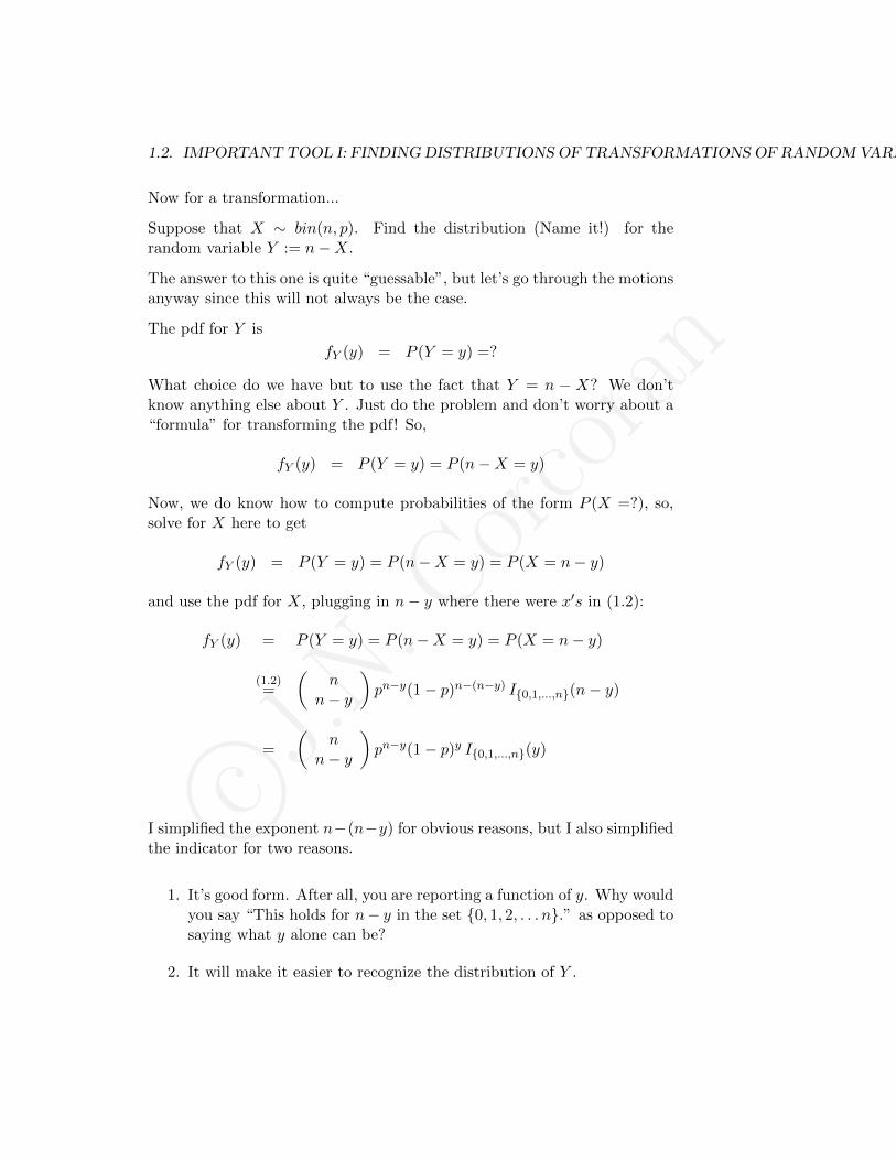
c©J.N.Corcoran
An Introduction to Mathematical Statistics
Course notes for APPM/MATH 4/5520
Fall 2014
by J.N. Corcoran
University of Colorado, Boulder.1
September 8, 2014
1Postal Address: Department of Applied Mathematics, University of Colorado,Boulder, CO 80309-0526, USA; email: [email protected]

c©J.N.Corcoran
2
Congratulations on deciding to take a course in ”MathStat.” And, if itwasn’t your decision, but instead some annoying or dreaded requirementdictated by your major, consider this your good fortune because MathStatseriously rocks.
The first secret I’m going to let you in on is that MathStat isn’t reallystatistics– it’s probability. Yes, there is a difference.
Probability is about the future.
Suppose you have an unfairly weighted coin that, if flipped, will result in“Heads” 57% of the time. Suppose that you are going to flip this coin10 times. What is the probability that you will see at least 7 Heads? Howmany Heads do you expect to see?
Did you catch all those future type words and phrases there?
Statistics, on the other hand, is about the past.
That is, suppose that you know next to nothing about the coin but youflipped it 10 times and observed the Heads/Tails data
H,H, T, T, T,H,H, T,H,H.
You can use statistics to attempt figure out (albeit with some uncertainty)whether or not the coin was fair in the first place and what that single flipHeads probability might have been.
Do you see how statistics is about looking back to figure out what was goingon with the coin?
Much of the subject of statistics is about “reverse engineering” the datagenerating process in the case that the process involves some randomnessor probability. Probability can stand alone as a subject, but in order to dostatistics we need to understand probability.
Mathematical Statistics is the probability needed to do statistics.
So you see, you have really enrolled yourself in a probability course andnot a statistics course. MathStat is a specialized area of probability and
c©J.N.Corcoran
3
before you can learn it you need to first know some basics. This is whya probability course, such as APPM 3570 (Applied Probability) or MATH4510 (Introduction to Probability Theory) is an important prerequisite.
Statistics, on the other hand, is not a prerequisite for this course, but ifyou’ve studied or used statistical analysis techniques, be prepared to seesome really cool connections this semester. If you’ve ever had a course instatistical analysis where you’ve estimated things (for example averages ormedians) or performed hypothesis tests that involved looking numbers up in,for example, “t-tables”, this course will tell you why doing those things wasmeaningful, when those techniques actually apply to a problem, and whatdo do if they don’t. Mathematical Statistics is an intense theoretical coursein which sometimes even the link to the “data stuff” will seem completelyobscured, but it is, in a word, beautiful.
These notes are designed for a course in the department of Applied Mathe-matics at the University of Colorado, Boulder. The course is cross-listed forgraduate students and senior undergraduates. The prerequisite is a basicundergraduate probability course. As the audience background has beenvaried, and adherence to prerequisites is often tenuous, I have included a“Preliminaries” chapter that may turn more advanced students, who havestumbled on to these notes from the web, off with its simplicity. Rest as-sured that things will ramp up quickly after that and that many will wantto skip the first chapter altogether. (It may still be useful to skim throughfor the purpose of picking up notation though.) I believe that these notesare well suited for a graduate course in Mathematical Statistics even in apure Statistics Department, where I have also had the experience of teachingMathStat. It includes many advanced concepts, examples, and challengingproblems.
On a final note, for maximum success in learning MathStat, or any mathe-matical subject for that matter, DO NOT TRY TO MEMORIZE THINGS!I always tell people that I ended up a mathematician because I have an awfulmemory. On a history exam, if you don’t know who did what and in whatyear, you are out of luck. Mathematics, however, comes from inside of you.If you’re stuck on a problem on a math exam, as long as you stay calm andkeep breathing, you can figure it out. (Always breathe!) If mathematicsdoesn’t “come naturally” to you, I’d urge to you to take the extra time andeffort to really understand the basics of a subject at the beginning of thesemester. It will be smooth sailing after that initial period and overall youwill spend a lot less time on your MathStat homework. I’ve dealt with a lot

c©J.N.Corcoran
4
of “mathphobes” over the years, and time and time again I’ve watched theones who take this advice eventually no longer need my help and go on tofocus on other things from “other classes” to “a life” while the others staya slave to my extended office hours right up to the final exam! Along thesesame lines, all of us are guilty at some point or another of searching theweb and/or a giant stack of books from the library for examples similar toa homework problem. The next time you do that, try keeping track of allthat time you spent that was not spent solving the problem.
“Just do it.” Cheesy? Absolutely, but also very true!
J.N. Corcoran
c©J.N.Corcoran
Contents
0 Probability Preliminaries 1
0.1 Between Zero and One . . . . . . . . . . . . . . . . . . . . . . 1
0.2 Counting . . . . . . . . . . . . . . . . . . . . . . . . . . . . . 3
0.2.1 Things in a Row . . . . . . . . . . . . . . . . . . . . . 3
0.2.2 Choosing Things: Order is Important . . . . . . . . . 5
0.2.3 Choosing Things: Order is Not Important . . . . . . . 7
0.3 Sample Spaces, Events, and Some Simple Probabilities . . . . 9
0.4 Some Very Brief Words About Independence and “Disjointness” 11
0.5 A Brief Review of Random Variables, PDFs, and CDFs . . . 14
0.5.1 Random Variables, the Bernoulli Distribution, and aSquiggly Line . . . . . . . . . . . . . . . . . . . . . . . 14
0.5.2 PDFs for Discrete Random Variables and the Geomet-ric Distribution . . . . . . . . . . . . . . . . . . . . . . 14
0.5.3 PDFs for Discrete Continuous Variables and the Ex-ponential Distribution . . . . . . . . . . . . . . . . . . 18
0.5.4 CDFs . . . . . . . . . . . . . . . . . . . . . . . . . . . 21
0.6 The Expected Value, Expectation, or Mean of a RandomVariable or a Distribution . . . . . . . . . . . . . . . . . . . . 24
0.7 The Variance of a Random Variable or a Distribution . . . . 28
0.8 Indicator Notation a Most Useful Appendix . . . . . . . . . . 30
i
c©J.N.Corcoran
ii CONTENTS
0.9 Joint PDFs, Marginals, and Independence . . . . . . . . . . . 31
0.10 “Twisted” Indicators . . . . . . . . . . . . . . . . . . . . . . . 38
1 MathStat Preliminaries: Four Important Tools for Mathe-matical Statistics 41
1.1 Wait. Where are we going? . . . . . . . . . . . . . . . . . . . 41
1.2 Important Tool I: Finding Distributions of Transformationsof Random Variables . . . . . . . . . . . . . . . . . . . . . . . 45
1.2.1 The Discrete Case and the Binomial Distribution . . . 45
1.2.2 The Continuous Case and the Gamma Distribution . . 49
1.3 Important Tool II: Bivariate Transformations . . . . . . . . . 55
1.3.1 The Beta Distribution . . . . . . . . . . . . . . . . . . 59
1.4 Important Tool II: Mins and Maxes . . . . . . . . . . . . . . 60
1.4.1 The Distrbution of a Minimum by Example . . . . . . 60
1.4.2 “Order Statistics” Notation . . . . . . . . . . . . . . . 61
1.4.3 PDFs for Minimums and Maximums . . . . . . . . . . 62
1.5 Important Tool IV: Moment Generating Functions (MGFs) . 64
1.5.1 The Expectation of a Function of X . . . . . . . . . . 65
1.5.2 Finding MGFs and the Poisson Distribution . . . . . . 68
1.5.3 Finding Moments . . . . . . . . . . . . . . . . . . . . . 70
1.5.4 The MGF Uniquely Identifies the Distribution . . . . 72
2 Qualities of Estimators: Defining Good, Better, and Best 75
2.1 Notation, Statistics, and Unbiasedness . . . . . . . . . . . . . 77
2.2 Expectation, Variance, and Covariance Review . . . . . . . . 78
A Tables of Distributions 79
B The Jacobian and a Change of Variables 83

c©J.N.Corcoran
CONTENTS iii
B.1 The Jacobian . . . . . . . . . . . . . . . . . . . . . . . . . . . 83
B.2 A Bivariate Transformation . . . . . . . . . . . . . . . . . . . 85
B.3 More Variables . . . . . . . . . . . . . . . . . . . . . . . . . . 86

c©J.N.Corcoran
iv CONTENTS
c©J.N.Corcoran
Chapter 0
Probability Preliminaries
This chapter is very elementary and is not at all representative of the overalllevel of these notes. This chapter is also a strange sort of introductionto probability in its coverage. Some very basic central concepts and evennotation for understanding probability are completely absent. Instead, itcontains only the bare minimum of topics needed in order to understand thesubsequent chapters. For those students who insist on trying mathematicalstatistics without a basic probability background, this should help. Forothers already familiar with things like random variables,“pdfs”, “cdfs”, andexpectations, it may be helpful to only skim Sections 0.1 through 0.7 sincethey will serve to establish some basic terminology and notation. Sections0.8-0.10 are recommended reading for everyone!
0.1 Between Zero and One
If you flip a “fair” coin, what is the probability that it will come up “heads”?
Most people have at least a sense of what this question is asking withoutany formal training in probability. Many will use the words “probability”and “chance” interchangeably and say:
“There is a 50 percent chance of it coming up heads.”
This is not wrong but, formally, in mathematics
1

c©J.N.Corcoran
2 CHAPTER 0. PROBABILITY PRELIMINARIES
Probability is a number between 0 and 1.
So, the more precise answer to the original question is 1/2 or 0.5.
If you roll a “fair” six-sided die, what is the probability that you will get a5?
In the case of the coin and now the die, the word “fair” is there to say thatthere is nothing funny going on. The coin isn’t warped, the die isn’t shavedor repainted with extra dots, and the acts of flipping and rolling are notdone in a way that favors one outcome over another. For the coin, the twooutcomes “heads” and “tails” are equally likely, and for the die, the sixoutcomes are equally likely.
To answer the question, since the outcome we care about (getting a 5) isone outcome out of six equally likely outcomes, the probability of getting a5 is 1/6.
If you roll a fair six-sided die, what is the probability that you will get eithera 5 or a 6?
Since there are now 2 outcomes out of 6 equally likely outcomes that wecare about, the answer is 2/6 or 1/3.
In the case of equally likely outcomes to anexperiment, the probability that a certain event
occurs is
the number of outcomes in the event of interest
divided by
the total number of possible outcomes.
c©J.N.Corcoran
0.2. COUNTING 3
Thus, in order to compute probabilities in the case of equally likely outcomes,it is important for us to be able to count things.
0.2 Counting
0.2.1 Things in a Row
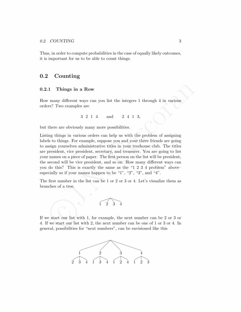
How many different ways can you list the integers 1 through 4 in variousorders? Two examples are
3 2 1 4 and 2 4 1 3,
but there are obviously many more possibilities.
Listing things in various orders can help us with the problem of assigninglabels to things. For example, suppose you and your three friends are goingto assign yourselves administrative titles in your treehouse club. The titlesare president, vice president, secretary, and treasurer. You are going to listyour names on a piece of paper. The first person on the list will be president,the second will be vice president, and so on. How many different ways canyou do this? This is exactly the same as the “1 2 3 4 problem” above–especially so if your names happen to be “1”, “2”, “3”, and “4”.
The first number in the list can be 1 or 2 or 3 or 4. Let’s visualize them asbranches of a tree.
1 2 3 4
If we start our list with 1, for example, the next number can be 2 or 3 or4. If we start our list with 2, the next number can be one of 1 or 3 or 4. Ingeneral, possibilities for “next numbers”, can be envisioned like this
1
2 3 4
2
1 3 4
3
1 2 4
4
1 2 3
c©J.N.Corcoran
4 CHAPTER 0. PROBABILITY PRELIMINARIES
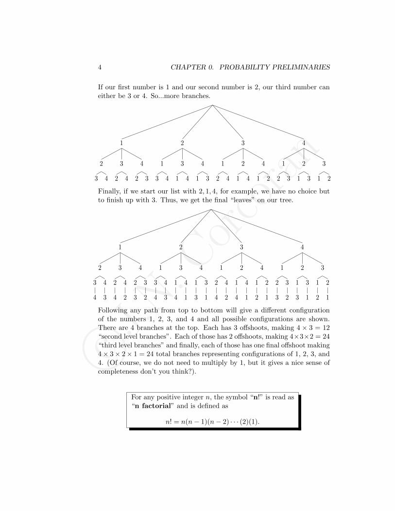
If our first number is 1 and our second number is 2, our third number caneither be 3 or 4. So...more branches.
1
2
3 4
3
2 4
4
2 3
2
1
3 4
3
1 4
4
1 3
3
1
2 4
2
1 4
4
1 2
4
1
2 3
2
1 3
3
1 2
Finally, if we start our list with 2, 1, 4, for example, we have no choice butto finish up with 3. Thus, we get the final “leaves” on our tree.
1
2
3
4
4
3
3
2
4
4
2
4
2
3
3
2
2
1
3
4
4
3
3
1
4
4
1
4
1
3
3
1
3
1
2
4
4
2
2
1
4
4
1
4
1
2
2
1
4
1
2
3
3
2
2
1
3
3
1
3
1
2
2
1
Following any path from top to bottom will give a different configurationof the numbers 1, 2, 3, and 4 and all possible configurations are shown.There are 4 branches at the top. Each has 3 offshoots, making 4 × 3 = 12“second level branches”. Each of those has 2 offshoots, making 4×3×2 = 24“third level branches” and finally, each of those has one final offshoot making4× 3× 2× 1 = 24 total branches representing configurations of 1, 2, 3, and4. (Of course, we do not need to multiply by 1, but it gives a nice sense ofcompleteness don’t you think?).
For any positive integer n, the symbol “n!” is read as“n factorial” and is defined as
n! = n(n− 1)(n− 2) · · · (2)(1).
c©J.N.Corcoran
0.2. COUNTING 5
From the trees above, we have seen that the number of ways to arrange 4distinct numbers (people/objects/things) is 4! = (4)(3)(2)(1) = 24.
In general,
n! = the number of ways to arrange n distinct objects.
From our little tree drawing experiment, we have learned at least two otherthings. First, if the numbers can be “reused”, the number of branches willnot decrease. For example, if we roll a fair 6-sided die 4 times we could seeoutcomes like
3 5 3 4 and 2 1 1 1.
The total number of possible outcomes will be 6 (first branches) times 6(second branches) times 6 (third branches) times 6 (fourth branches), for atotal of 64 = 1296 outcomes.
At this point I could make another box with a factoid in it saying somethinglike: “If we perform an experiment with k trials and with n possible out-comes for each trial, we have a total of nk possible outcomes for the entireexperiment.” However, I won’t and you shouldn’t either. If you arememorizing things for a math class (outside of definitions), the class willget more and more and more difficult as you pile up information in yourhead and eventually struggle to access it. If you are memorizing things for amath class, you are going to be thrown off when problems have only subtledifferences from ones you’ve already seen or solved. On the other hand, ifyou understand and think about what you’re doing at each step, the classwill get easier and easier even as the material gets more complex!
0.2.2 Choosing Things: Order is Important
Here is the second thing we have learned from our “tree experiment”. Sup-pose we have to choose 2 numbers out of our 4 numbers and that “order isimportant”. This means that
1 4 is different from 4 1.
c©J.N.Corcoran
6 CHAPTER 0. PROBABILITY PRELIMINARIES
For the four people in the treehouse club, this scenario could come up if youwant to choose only a president and a vice president. You could write twonames down and the first in your list will be president, while the second willbe vice president. If, as before, the treehouse club’s members names are 1,2, 3, and 4, the choice
1 4
means that person 1 is president and person 4 is vice president, while thedifferent choice
4 1
means that person 4 is president and person 1 is vice president.
Since you have 4 choices to put in the first position (envisioned as firstbranches of a tree) and then 3 leftover people to choose for the secondposition (second branches), you have a total of 4× 3 = 12 possible ways toassign names to the president and vice president positions in your list.
That was easy enough, but it will be useful to be able to come up with thisnumber using factorials. You might have noticed that
12 = 4 · 3 =4 · 3 · 2 · 1
2 · 1=
4!
2!,
but let’s discuss the logic behind this. The point will be a little more clearif we increase the number of treehouse members to five. (The only reasonI didn’t start with five in the first place is because the tree diagram wouldhave been really wide and too cramped for these pages!)
Suppose there are five members of the treehouse club and that their namesare 1, 2, 3, 4, and 5. Further suppose that we want to know how manydifferent ways we can choose a president and a vice president. We could listall of the members in various orders and choose the first two people in thelist to be the president and vice president, respectively. For example, onepossible listing of members is
4 2 5 3 1.
For this listing, 4 will be president and 2 will be vice president.
Another possible listing of members is
2 4 5 3 1.
In this case, 2 will be president and 4 will be vice president.
c©J.N.Corcoran
0.2. COUNTING 7
In all, there are 5! = 120 possible listings of these 5 people, but for ourpurpose of choosing a president and vice president some are redundant. Forexample
4 2 5 3 1 and 4 2 1 3 5
will give the same results for our election. In fact, for this 5 person listingmethod, we will get the result of 4 as president and 2 as vice president3! = 6 different times since there are 3! different ways to arrange the threesuperfluous numbers 1, 3, and 5. Furthermore, we will get every particularpresident and vice president combinations redundantly listed 3! = 6 differenttimes. So, we need to divide the 120 possibly ways to list 5 people by 6. Insummary, the number of ways to choose 2 people (numbers/objects/things)from 5 people (numbers/objects/things) when order is important is
5!
3!=
120
6= 20.
In general, the number of ways to choose k objects out of nobjects when order is important is n!/(n− k)!.
What we have just done is to count the number of “permutations” of kobjects out of n objects. The quantity we came up with in the end isdenoted in many different ways. One of the most popular is nPk. That is,
nPk := n!/(n− k)!.
You will not need this notation in this course or to understand the rest ofthese notes. If needed, we will figure out how to choose k things out of nthings with logic, just as we did in the treehouse example!
0.2.3 Choosing Things: Order is Not Important
Suppose now that we want to choose two people from our five membertreehouse club to fix the ladder. How many different possible “ladder fixingcommittees” are there? If we were listing out pairs of people, the order isnot important because having 1 and 4 fix the ladder is the same as having4 and 1 fix the ladder.
c©J.N.Corcoran
8 CHAPTER 0. PROBABILITY PRELIMINARIES
We will take the same approach as in the previous section, where we list outall five names and then take the first two names for our committee.
There are 5! = 120 ways to list the 5 names. One possibility is
4 2 5 3 1.
This particular listing of names will give us a committee consisting of 4and 2. As before, the order of the last 3 people is irrelevant and, using allpossible listings, we will get 4 and 2 for our committee 3! different ways. So,we should divide 5! by 3! to account for this redundancy. At this point, wehave 5!/3! lists we care about.
Note that, we still have some redundancy since the outcome
4 2 5 3 1
is now the same as
2 4 5 3 1.
Both of these outcomes mean that our ladder committee consists of 4 and2. In fact, every pair of people will end up being listed 2 ways. (Note that,for ease of generalization, the number of ways to list 2 people is 2! = 2.)
So, for our 5!/3! surviving lists, we need to divide by 2!. In summary, thenumber of ways to choose 2 people (numbers/objects/things) from 5 people(numbers/objects/things) when order is not important is
5!/3!
2!=
5!
2! 3!.
In general, the number of ways to choose k objects out of nobjects when order is not important is
n!
k! (n− k)!.
What we have just done is to count the number of “combinations” of kobjects out of n objects. This quantity is almost always denoted by the
c©J.N.Corcoran
0.3. SAMPLE SPACES, EVENTS, AND SOME SIMPLE PROBABILITIES9
symbol
(nk
). That is
(nk
):=
n!
k! (n− k)!.
This symbol is read “n choose k” and we will use it a lot!
0.3 Sample Spaces, Events, and Some Simple Prob-abilities
In probability, we typically use capital Roman letters like A, B and C, forexample to denote “events” which are collections of outcomes from someexperiment.
Suppose we perform the fabulously exciting experiment of flipping a faircoin 3 times. Using what I hope is an obvious notation for the sequences of“Heads” and “Tails” the eight possible outcomes are
HHH,HHT,HTH, THH,HTT, THT, TTH, TTT.
The set of all possible outcomes of experiment is known asthe sample space of the experiment.
We will use the symbol Ω to denote the sample space of an experiment.
For this example we would write
Ω = HHH,HHT,HTH, THH,HTT, THT, TTH, TTT.
Let us define the event called “A” as the one where we see at least one“Heads” in our experiment. Formally, we have defined
A = HHH,HHT,HTH, THH,HTT, THT, TTH
which is a subset of the sample space Ω.
c©J.N.Corcoran
10 CHAPTER 0. PROBABILITY PRELIMINARIES
What is the probability that the event A occurs? That is, if we are goingto flip a fair coin 3 times, what is the probability that we will see at least 1“Heads”?
We will use P (A) to denote the probability that the event Aoccurs.
Since 7 out of the 8 possible outcomes are included in the set A, this proba-bility should be very high. This conclusion though is based on the idea thatmost outcomes are in A, but, it is also based on the idea that the coin is“fair”. If the coin were severely bent or weighted in such a way that “Tails”comes up 99 percent of the time then we should expect that it is somewhatunlikely that we will see at least 1 “Heads”!
Because Heads and Tails are “equally likely” for a fair coin, the three tossoutcomes, HHH, HHT , etc. are also equally likely. You might be think-ing that outcomes like HHH or TTT are less likely than the others for afair coin. To make this even more dramatic, imagine tossing the coin 20times. Shouldn’t the outcome of 20 Tails be very unlikely? The fact ofthe matter is that it will not be any more unlikely than any other spe-cific sequence! Just imagine flipping 20 times with the goal of gettingHTTHTHTHTHHTHTHTHTHT . This would be hard to do! Simi-larly getting the elusive royal flush poker hand (ace, king, queen, jack andten all in the same suit) is no more difficult than getting the hand that isexactly the 3 of clubs, 10 of diamonds, 7 of spades, 3 of hearts, and thejack of spades. Actually, it is easier since there are 4 different possible royalflushes– one for each suit.
Back to the question... If we flip a fair coin 3 times, what is P (A), theprobability that we will see at least 1 Heads? Since the 8 outcomes in Ω areequally likely and since there are 7 outcomes where we see at least 1 Heads,we have a “7 out of 8 chance” of seeing at least one Heads. That is,
P (A) = 7/8.
It may also be convenient for us to write this out as
P (HHH,HHT,HTH, THH,HTT, THT, TTH) = 7/8.

c©J.N.Corcoran
0.4. SOME VERY BRIEFWORDS ABOUT INDEPENDENCE AND “DISJOINTNESS”11
In general, if Ω is a set of equally likely outcomes of an ex-periment and A is a subset of Ω,
P (A) =# outcomes in A
# outcomes in Ω.
This is why establishing some counting techniques in the pre-vious sections was important.
Example:
If you randomly select 5 cards from a deck of 52 cards, what is the probabilitythat you will get a royal flush?
Answer: First of all, note that order is not important here. If you are playingpoker, you might be excited to have 3 aces in your hand but you certainlywouldn’t care that one of them was near your thumb and the other twowere closer to your pinky. Therefore, as we learned in Section 0.2.3, the
total number of 5 card hands is given by
(525
).
Since every 5 card hand is equally likely and since there are exactly 4 handsthat are a royal flush (ace, king, queen, jack, and 10 in the same suit andthere are 4 suits), we have that
P ( royal flush ) = 4
/(525
)Incidentally, after working out the factorials, this is 4/2, 598, 960 = 1.539077×10⁻⁶! (← That is an exclamation point for excitement and not another fac-torial!) (← That is an exclamation point...)
0.4 Some Very Brief Words About Independenceand “Disjointness”
Independence
In the previous section, we considered flipping a fair coin 3 times. Thepossible out comes were
Ω = HHH,HHT,HTH, THH,HTT, THT, TTH, TTT.

c©J.N.Corcoran
12 CHAPTER 0. PROBABILITY PRELIMINARIES
Although it wasn’t stated, the implication here is that the coin is flippedin a fair way and that the flips are independent. That is, what happens onthe second flip, for example, does not depend on what happened on the firstflip. (For example, we are not flipping the coin with a spatula! T , H, T , H,T , H, T , · · ·)
What is the probability of seeing the result HTH? Based on the previoussection, and because the outcomes are equally likely, we know by countingthat the answer is 1/8. in this section we assume that we don’t want tobother writing out or counting all the possible outcomes.
Note that the “event” HTH means that we got Heads on the first toss of thecoin, Tails on the second toss, and Heads on the third toss. Furthermore,note that the coin doesn’t care about what toss we are on at any point so
P ( Heads on any one toss ) = 1/2
andP ( Tails on any one toss ) = 1/2.
Note that
P (HTH) =1
8=
1
2· 1
2· 1
2.
In general, if A and B are independent events
P (A and B) = P (A) · P (B).
Applying this (generalizing to 3 events) to our problem, since the flips areindependent, we have that
P (HTH) = P ( Heads on the first flip ANDTails on the second flip ANDHeads on the third flip )
= P ( Heads on the first flip)·P (Tails on the second flip)·P (Heads on the third flip )
= 12 ·
12 ·
12 = 1
8 .
c©J.N.Corcoran
0.4. SOME VERY BRIEFWORDS ABOUT INDEPENDENCE AND “DISJOINTNESS”13
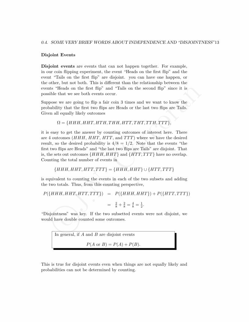
Disjoint Events
Disjoint events are events that can not happen together. For example,in our coin flipping experiment, the event “Heads on the first flip” and theevent “Tails on the first flip” are disjoint. you can have one happen, orthe other, but not both. This is different than the relationship between theevents “Heads on the first flip” and “Tails on the second flip” since it ispossible that we see both events occur.
Suppose we are going to flip a fair coin 3 times and we want to know theprobability that the first two flips are Heads or the last two flips are Tails.Given all equally likely outcomes
Ω = HHH,HHT,HTH, THH,HTT, THT, TTH, TTT,
it is easy to get the answer by counting outcomes of interest here. Thereare 4 outcomes (HHH, HHT , HTT , and TTT ) where we have the desiredresult, so the desired probability is 4/8 = 1/2. Note that the events “thefirst two flips are Heads” and “the last two flips are Tails” are disjoint. Thatis, the sets out outcomes HHH,HHT and HTT, TTT have no overlap.Counting the total number of events in
HHH,HHT,HTT, TTT = HHH,HHT ∪ HTT, TTT
is equivalent to counting the events in each of the two subsets and addingthe two totals. Thus, from this counting perspective,
P (HHH,HHT,HTT, TTT) = P (HHH,HHT) + P (HTT, TTT)
= 28 + 2
8 = 48 = 1
2 .
“Disjointness” was key. If the two subsetted events were not disjoint, wewould have double counted some outcomes.
In general, if A and B are disjoint events
P (A or B) = P (A) + P (B).
This is true for disjoint events even when things are not equally likely andprobabilities can not be determined by counting.
c©J.N.Corcoran
14 CHAPTER 0. PROBABILITY PRELIMINARIES
0.5 A Brief Review of Random Variables, PDFs,and CDFs
0.5.1 Random Variables, the Bernoulli Distribution, and aSquiggly Line
A random variable is a “mapping” from the set if possible outcomes of anexperiment, involving some randomness or probability, to numbers.
Example:
Flip a, possibly unfair, coin that has some probability p of coming up“Heads” and probability 1 − p of coming up “Tails”, where p is some fixednumber in the interval [0, 1].
Define
X =
1 , if “Heads”0 , if “Tails”
Then X is a random variable that takes the value 1 with probability p and0 with probability 1− p.
This (0/1) type of random variable comes up so often that it gets a name.
X is called a Bernoulli random variable with parameter p. Alter-natively, we say that X has a Bernoulli distribution with parameterp.
Our shorthand notation for this will be to write
X ∼ Bernoulli(p).
Sometimes you might instead see X ∼ Bern(p). The symbol “∼” should beread as “has the distribution”.
0.5.2 PDFs for Discrete Random Variables and the Geomet-ric Distribution
There are two very important functions associated with random variables.One is called the
c©J.N.Corcoran
0.5. A BRIEF REVIEWOF RANDOMVARIABLES, PDFS, AND CDFS15
probability density function or “pdf”
and the other is called the
cumulative distribution function or “cdf”.
Most of the random variables we will talk about in this course will be ei-ther discrete (taking on possible values from a discrete set) or continuous(taking on possible values in a continuum). This section is about pdfs fordiscrete random variables. Please note that many authors use the termi-nology “probability density function” and the acronym “pdf” only whentalking about continuous random variables and, in the discrete case, referto the function about to be defined here as a probability mass function(pmf). In these notes, we will not make this distinction.
Definition:
Let X be a discrete random variable.
The probability density function (pdf) for a discrete random variableX is the function f defined by
f(x) = P (X = x).
The right-hand side there is used to denote the probability that X takes onthe specific value x.
Important Note:In probability and statistics, it is customary to use capital letters to denoterandom variables and lower case letters to denote specific fixed values.
Example:
Suppose that X ∼ Bernoulli(p). What is the pdf of X?

c©J.N.Corcoran
16 CHAPTER 0. PROBABILITY PRELIMINARIES
Answer:
Since P (X = 1) = p and P (X = 0) = 1 − p, by our definition of the pdf,we have that f(1) = p and f(0) = 1− p. Furthermore, f(2.7), for example,is f(2.7) = P (X = 2.7) = 0, since X can only take on values in 0, 1. Insummary, the pdf is
f(x) =
1− p , x = 0p , x = 10 , otherwise.
In mathematics, we usually call the region on which a function is defined thedomain of the function. Noticed that the above pdf is defined everywhere(for all real numbers) but is only really “interesting” at the points x = 0and x = 1. In general, the region where a function is non-zero is called thesupport of the function. If you use these terms interchangeably, so be it–it is not the end of the world, but really they have different meanings.
Here is a new “named” distribution for you.
Example:
Consider an experiment consisting of a sequence of independent trials ofsomething where each trial can have only two possible outcomes, usuallylabeled as “success” and “failure”.
Let p (0 ≤ p ≤ 1) be the probability of “success” on any one trial.
Let
X = # trials until the first success.
Then the possible values for X are 1, 2, 3, . . ..
For example, in an idealized world, you might imagine someone shootingbaskets in basketball and X as the number of tries they have to take untilthey make a basket. (In real life though, the assumptions that the successprobability is constant for all trials and the trials are independent wouldprobably be violated as the person could be learning from each failed attemptand making adjustments to get better or maybe their arms are tired andthey are getting worse!)
c©J.N.Corcoran
0.5. A BRIEF REVIEWOF RANDOMVARIABLES, PDFS, AND CDFS17
Question: What is the pdf for X?
Answer:
Note thatP (X = 1) = P ( success on first trial ) = p.
Continuing,
P (X = 2) = P ( failure on 1st trial AND success on 2nd trial ).
By independence of the trials, this is
P (X = 2) = P ( failure on 1st trial ) · P ( success on second trial )
= (1− p) · p.
Similarly,
P (X = 3) = P ( “F” on 1st trial AND “F” on 2nd trial AND “S” on 3rd trial )
indep= P ( “F” on 1st trial ) · P ( “F” on 2nd trial ) · P ( “S” on 3rd trial )
= (1− p) · (1− p) · p = (1− p)2 · p.
A pattern is forming...
P (X = x) = (1− p)x−1 · p
for x = 1, 2, 3, . . ..
Since P (X = x) = 0 for x not in 1, 2, 3, . . ., we conclude that the pdf is
f(x) =
(1− p)x−1 · p , x = 1, 2, 3 . . .0 , otherwise.
Again we have happened across a type of random variable that is so commonit gets a name. X is said to be a geometric random variable withparameter p. Alternatively, we say thatX has a geometric distribution.We write
X ∼ geom(p).

c©J.N.Corcoran
18 CHAPTER 0. PROBABILITY PRELIMINARIES
Note that, using the same set up with successes and failures on independenttrials, some people will define the geometric random variable as
X = # failures before the first success.
Now, if we see a success on the first trial, X will take the value 0. It is easyto adjust what we did above to show that the pdf is now
f(x) =
(1− p)x · p , x = 0, 1, 2, . . .0 , otherwise.
Although it is not standard notation, for this course I will write
X ∼ geom0(p)
to denote the random variable having the geometric distribution that startsfrom 0 and
X ∼ geom1(p)
to denote the random variable having the geometric distribution that startsfrom 1.
0.5.3 PDFs for Discrete Continuous Variables and the Ex-ponential Distribution
Let X be a continuous random variable.
The probability density function (pdf) for a continuousrandom variable X is a function f under which area repre-sents probability.
For example, if the continuous random variable X has the pdf depicted inFigure 1(a), then the probability P (a < X ≤ b) is the shaded region depictedin Figure 1(b). This is computed as the integral
P (a < X ≤ b) =
∫ b
af(x) dx.

c©J.N.Corcoran
0.5. A BRIEF REVIEWOF RANDOMVARIABLES, PDFS, AND CDFS19
Figure 1: A pdf for a Continuous Random Variable
Since the area of the vertical lines at the boundaries of the region have areazero, we can put them in or take them out without changing the area of theshaded region. Thus,
P (a < X ≤ b) = P (a ≤ X ≤ b) = P (a ≤ X < b) = P (a < X < b).
Furthermore, for any a,
P (X = a) =
∫ a
af(x) dx = 0.
The pdf described how the probabilities associated with a random variableare “distributed” over the real line. Where is most of the area under thecurve piled up? That is where you are most likely to observe the randomvariable if you record an actual “realization” (numerical observation) of itin the future. Thus, we will often talk about the pdf associated with a“distribution” instead of talking about the random variable itself.
For any pdf f , we must have
• f(x) ≥ 0 for all x
and, for a pdf for a continuous distribution we must have

c©J.N.Corcoran
20 CHAPTER 0. PROBABILITY PRELIMINARIES
•∫∞−∞ f(x) dx = 1
Example:
Suppose you are standing near the door of a grocery store watching cus-tomers arrive.
Suppose further that
1. the arrival rate is a constant 15.2 people per minute, and
2. the number of arrivals in non-overlapping periods of time are indepen-dent.
(Yes, it may not be realistic to have the arrival rate be constant all day.Consider it an overly simplistic model but a model nonetheless!)
Let
X = the time (in minutes) between any two consecutive arrivals.
The we can show (take APPM 4/5560!) that this continuous random vari-able X has the pdf
f(x) =
15.2e−15.2x , x ≥ 00 , x < 0.
X is said to be an exponential random variable with rate 15.2 or tohave an exponential distribution with rate 15.2.
We will writeX ∼ exp(rate = 15.2).
Note that, if people are arriving at a rate of 15.2 per minute, then, onaverage, the time between arrivals is 1/15.2 minutes. In general, if peopleare arriving at a rate of λ per minute, then the mean “interarrival time” is1/λ minutes.
We have
X ∼ exp(rate = λ) ⇒ f(x) =
λe−λx , x ≥ 00 , x < 0.
c©J.N.Corcoran
0.5. A BRIEF REVIEWOF RANDOMVARIABLES, PDFS, AND CDFS21
However, many people specify this model in terms of the mean interarrivaltime and call that mean λ. This would correspond to a rate of 1/λ and sowe write
X ∼ exp(mean = λ) ⇒ f(x) =
1λe−x/λ , x ≥ 0
0 , x < 0.
Unfortunately, many texts use the notation X ∼ exp(λ) and it is up to youto look through earlier parts of the book to figure out which of these two pdfsthey are talking about. In this course, we will almost always be thinking ofit in terms of the rate parameter and I will always explicitly write “rate =λ”.
0.5.4 CDFs
The acronym cdf stands for cumulative distribution function.
The cdf of a random variable X is usually denoted by F (x) and isdefined as
F (x) = P (X ≤ x).
This definition holds for both discrete and continuous random variables.
Example: (Discrete)
Suppose that X ∼ geom0(p). For any integer x,
F (x) = P (X ≤ x) =∑u≤x
P (X = u)geom=
x∑u=0
P (X = u)
=x∑u=0
(1− p)up = px∑u=0
(1− p)u
This is a finite geometric sum. Recall first the infinite geometric sum
∞∑n=0
rn =1
1− rif |r| < 1.

c©J.N.Corcoran
22 CHAPTER 0. PROBABILITY PRELIMINARIES
The finite geometric sum,∑N
n=0 rn is similar in the denominator and has
the formN∑n=0
rn =?
1− r.
Writing the left side out as 1 + r + r2 + · · ·+ rN , we see that
? = (1− r)(1 + r + r2 + · · ·+ rN )
= (1 + r + r2 + · · ·+ rN )− r(1 + r + r2 + · · ·+ rN )
= (1 + r + r2 + · · ·+ rN )− (r + r2 + r3 + · · ·+ rN+1)
= 1− rN+1.
Thus,N∑n=0
rn =1− rN+1
1− r.
Going back to the cdf for the geometric distribution, we have
F (x) = px∑u=0
(1− p)u
which is a finite geometric sum with r = 1− p and N = x. Therefore,
F (x) = p
x∑u=0
(1− p)u = p1− (1− p)x+1
1− (1− p)= 1− (1− p)x+1.
Here, we assumed that x was an integer. Because the distribution is integervalued, we have, for example that
F (5.6) := P (X ≤ 5.6) = P (X ≤ 5) = F (5) = 1− (1− p)6.
Because X only takes on non-negative integer values, we have that
F (0) = P (X ≤ 0) = 1− (1− p) = p = P (X = 0)
and that, for x < 0,F (x) = P (X ≤ x) = 0.
In summary, if X ∼ geom0(p), the cdf is
F (x) =
1− (1− p)bxc+1 , x ≥ 00 , x < 0
c©J.N.Corcoran
0.5. A BRIEF REVIEWOF RANDOMVARIABLES, PDFS, AND CDFS23
where b·c is the greatest integer function.
Example: (Continuous)
Suppose that X ∼ exp(rate = λ). For any x ≥ 0,
F (x) = P (X ≤ x) =∫ x−∞ f(u) du
=∫∞
0 λe−λu du = 1− e−λx.
Notice that the limits of integration changed because the pdf is 0 for x < 0.Technically, we have∫ x
−∞f(u) du =
∫ 0
−∞0 du+
∫ x
0λe−λu du
Since the exponential distribution only takes on positive values, we have, forx < 0, that F (x) = P (X ≤ x) = 0. In summary, the cdf for the exponentialdistribution with rate λ is
F (x) =
1− e−λx , x ≥ 00 , x < 0.
We have seen two examples of how to get from a distribution pdf to itscdf. Suppose we want to reverse the process. That is, given a cdf, can wecompute the associated pdf?
Discrete Case:
Rather than write out a formula, it is easiest to consider by example andon a case-by-case basis. Suppose, for example, that we are dealing with adistribution that takes on integer values. Then we can define the pdf at, say3 by
f(3) = P (X = 3) = P (X ≤ 3)− P (X ≤ 2) = F (3)− F (2).
Continuing this example, for general integer values of x, we can define
f(x) = P (X ≤ x)− P (X ≤ x− 1) = F (x)− F (x− 1).
c©J.N.Corcoran
24 CHAPTER 0. PROBABILITY PRELIMINARIES
We would also define f(x) = 0 whenever x is not an integer or if x is aninteger that is outside the support of the distribution.
In theory, it is easy to generalize this method of recovering the pdf from a cdffor discrete random variables that do not live on integers but the notationis kind of messy.
Continuous Case It is much easier to move from a cdf to a pdf in thecontinuous case. Because the cdf is defined as
F (x) =
∫ x
−∞f(u) du,
the Fundamental Theorem of Calculus gives us the following.
If X is a continuous random variable with cdf F (x), the pdf is
f(x) =d
dxF (X).
For example, for the exponential distribution with rate λ, the cdf is F (x) =1− e−λx for x ≥ 0. The pdf is therefore
f(x) =d
dxF (X) =
d
dx(1− e−λx) = λe−λx
for x ≥ 0.
0.6 The Expected Value, Expectation, or Mean ofa Random Variable or a Distribution
We will denote the expected value (also called the expectation or mean)of a random variable X as E[X].
The expected value of X is a probability weighted average.
c©J.N.Corcoran
0.6. THE EXPECTEDVALUE, EXPECTATION, ORMEANOF A RANDOMVARIABLE OR ADISTRIBUTION25
Example:
Suppose that X is discrete, taking values in 0, 1, 2 with probabilities
x 0 1 2
P (X = x) 0.2 0.7 0.1
Then
E[X] = (0)(0.2) + (1)(0.7) + (2)(0.1) = 0.9.
In general, for a discrete random variable X, the expected value is
E[X] =∑x
x · P (X = x) =∑x
x · f(x).
Technically, the sum is taken over all real numbers. (Note that a discreterandom variable is not restricted to integers!) However, we can also justsum over the support of the distribution which includes all x’s for whichf(x) = P (X = x) = 0.
Example:
Let X ∼ geom0(p). Find E[X].
Answer:
Since
f(x) =
(1− p)x−1 · p , x = 1, 2, 3 . . .0 , otherwise,
we have that
E[X] =∑xxf(x) =
∞∑x=0
x · (1− p)x · p.
Continuing,
E[X] =∞∑x=0
x · (1− p)x · p = p∞∑x=0
x(1− p)x = p∞∑x=1
x(1− p)x (1)
c©J.N.Corcoran
26 CHAPTER 0. PROBABILITY PRELIMINARIES
since the sum is zero when x = 0. Hmmmm... an infinite sum. The onlyone of those most of us can remember is the geometric sum
∞∑n=0
rn =1
1− rif |r| < 1
which can easily be adjusted to start from different places. For example
∞∑n=3
rn = r3∞∑n=3
rn−3 = r3∞∑n=0
rn = r3 · 1
1− r.
The sum in (1) sort of looks like a geometric sum with r = 1− p. The onlyproblem is that leading x. Check this out:
E[X] = p∞∑x=1
x(1− p)x = p(1− p)∞∑x=1
x(1− p)x−1.
Now the summand kind of looks like a derivative. Defining q = 1 − p, wemay rewrite it again as
E[X] = p(1− p)∞∑x=1
ddq q
x
= p(1− p) ddq∞∑x=1
qx
which is a nice geometric sum. Thus
E[X] = p(1− p) ddq∞∑x=1
qx
= p(1− p) ddqq
1−q
= p(1− p) (1−q)(1)−q(−1)(1−q)2
= p(1− p) 1(1−q)2 = p(1− p) 1
p2= 1−p
p
In summary, if X ∼ geom0(p),
E[X] =1− pp
.
c©J.N.Corcoran
0.6. THE EXPECTEDVALUE, EXPECTATION, ORMEANOF A RANDOMVARIABLE OR ADISTRIBUTION27
Now for a continuous example.
Example:
Suppose that X ∼ exp(rate = λ). Find E[X].
Answer:
Since the exponential distribution is a continuous distribution we must usethe integral definition for this expected value.
E[X] =∫∞−∞ x · f(x) dx
=∫∞−∞ x · λe
−λx · I(0,∞)(x) dx
=∫∞
0 x · λe−λx dx
Using integration by parts (∫u dv = uv−
∫v du) with u = x and dv = λe−λx,
we have
E[X] = −xe−λx∣∣∣∞0−∫ ∞
0(−e−λx) dx.
That first term certainly evaluates to 0 when we plug in x = 0. It is also 0 at∞ (technically a limit as x → ∞). This is because e−λx goes down to zerofaster than x blows up, but formally this can be shown using L’Hopital’sRule.
We are left with
E[X] =
∫ ∞0
eλx dx = − 1
λe−λx
∣∣∣∣∞0
= − 1
λ(0− 1) =
1
λ.
Remember, the expected value of a random variable (or, equivalently, of adistribution) is also known as its expectation or mean. The 1/λ that wefound here is consistent with our discussion of rates and means at the endof Section 0.5.3.
Notation:
c©J.N.Corcoran
28 CHAPTER 0. PROBABILITY PRELIMINARIES
A final point of notation. The mean or expected value of a random variableX is often denoted with the Greek letter µ. that is,
µ := E[X].
In the case of multiple random variables, say X and Y , a subscript becomesnecessary to distinguish the means,
µX = E[X] and µY = E[Y ].
While people would surely understand what you mean if you instead uselowercase subscripts as in µx and µy, this represents a really fundamentallack of understanding about what you are doing since lowercase Romanalphabet letters in statistics almost always refer to specific numbers and notrandom variables which can be thought of as “potential but yet unobservednumbers”. For the record, if c is a constant, then E[c] = c. You can thinkof c as an uninteresting random variable X where X = c with probability 1.Then E[c] = E[X] = c · P (X = c) = c · 1 = c. For example,
E[3] = 3
and, adhering to the convention of random variables being uppercase,
E[x] = x.
While we’re at it here, a mean µ is also a constant. When you compute anyexpectation you have already sort of “summed out” the probability. Thus,while we may have defined µ = E[X] for some random variable X, E[µ] willjust be µ again!
0.7 The Variance of a Random Variable or a Dis-tribution
We will denote the variance of a random variable X as V ar[X].
The variance of a random variable X is a measure of spreadabout its mean.

c©J.N.Corcoran
0.7. THE VARIANCE OF A RANDOMVARIABLE OR ADISTRIBUTION29
If we use µ to denote the mean E[X], then the variance of X is defined by
V ar[X] = E[(X − µ)2].
A variance is usually also denoted by the symbol σ2 with subscripting possi-ble if it becomes necessary to distinguish between the variances for differentrandom variables.
If you were devise your own measure of spread of a random variable X aboutits mean µ, you might use the expected distance
E[|X − µ|],
but we will see this semester that the above definition is in fact way moreconvenient from a mathematical perspective.
You may already be familiar with the expression
σ2 = V ar[X] = E[X2]− (E[X])2.
We will see in Section ?? that the expectation “operator” is in fact a linearoperator so that, for random variables X and Y and constants a and b, wehave
E[aX + bY ] = aE[X] + bE[Y ].
In particular,E[X + Y ] = E[X] + E[Y ]
and, taking b = −1,E[X − Y ] = E[X]− E[Y ].
With this in mind, we have that
V ar[X] = E[(X − µ)2]
= E[X2 − 2µX + µ2]
= E[X2]− 2µE[X]︸︷︷︸µ
+µ2 (µ is a constant)
= E[X2]− 2µ2 + µ2
= E[X2]− µ2
= E[X2]− (E[X])2.
c©J.N.Corcoran
30 CHAPTER 0. PROBABILITY PRELIMINARIES
0.8 Indicator Notation a Most Useful Appendix
We have three “named” distributions so far: the Bernoulli, the geomet-ric, and the exponential distributions. The most common (in my opinion)named distributions are summarized in Tables A.1 and A.2. We will even-tually talk about all of the columns in these tables. As of right now, thefirst four columns should make sense. They include names of distributions,corresponding pdfs, a description of the allowable parameter space (For ex-ample, p for the Bernoulli and geometric distributions is itself a probabilityand can range from 0 to 1.), and the mean (expected value) for each distri-bution. Each pdf in the tables includes an extra part involving an “I”. Thisis an indicator function which is defined as follows.
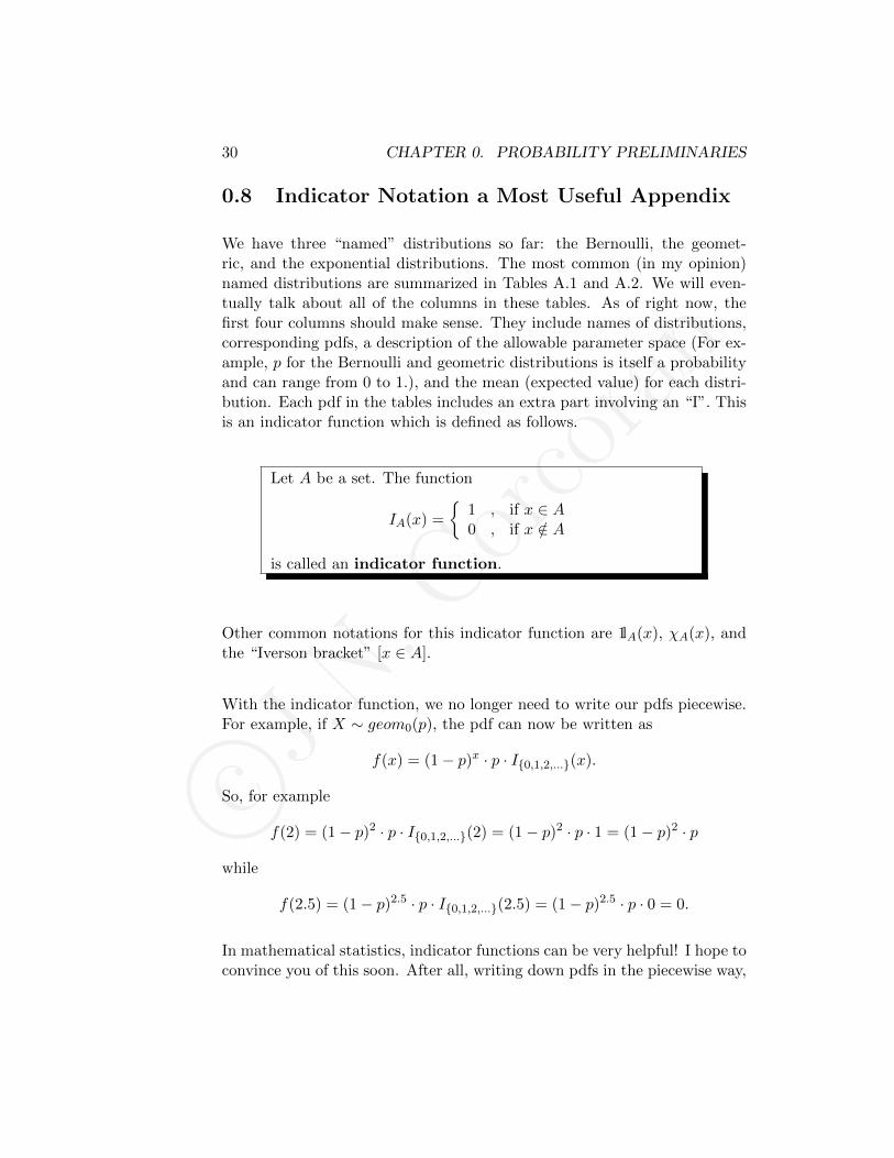
Let A be a set. The function
IA(x) =
1 , if x ∈ A0 , if x /∈ A
is called an indicator function.
Other common notations for this indicator function are 1lA(x), χA(x), andthe “Iverson bracket” [x ∈ A].
With the indicator function, we no longer need to write our pdfs piecewise.For example, if X ∼ geom0(p), the pdf can now be written as
f(x) = (1− p)x · p · I0,1,2,...(x).
So, for example
f(2) = (1− p)2 · p · I0,1,2,...(2) = (1− p)2 · p · 1 = (1− p)2 · p
while
f(2.5) = (1− p)2.5 · p · I0,1,2,...(2.5) = (1− p)2.5 · p · 0 = 0.
In mathematical statistics, indicator functions can be very helpful! I hope toconvince you of this soon. After all, writing down pdfs in the piecewise way,
c©J.N.Corcoran
0.9. JOINT PDFS, MARGINALS, AND INDEPENDENCE 31
where we say “and zero otherwise” is not very hard to do. Furthermore, wecould easily get away with just writing down the “important piece” of thepiecewise defined pdf and just leave it implied that it is “zero otherwise”.Indeed, I have other reasons for using indicator functions– the first of whichwe will see shortly. In the meantime, let’s just start getting used to themnow!
0.9 Joint PDFs, Marginals, and Independence
For discrete random variables X and Y , we define the jointpdf as
f(x, y) := P (X = x and Y = y)notation
= P (X = x, Y = y).
Note that the x and y are just place holding dummy variables. For example,
P (X = 1, Y = 3) = f(1, 3)
andP (X = w, Y = z) = f(w, z).
So, if it is necessary to be more specific about which random variables thejoint pdf belongs to, we might write it as fX,Y (x, y). Then, it is clear that
fX,Y (w, z) = P (X = w, Y = z).
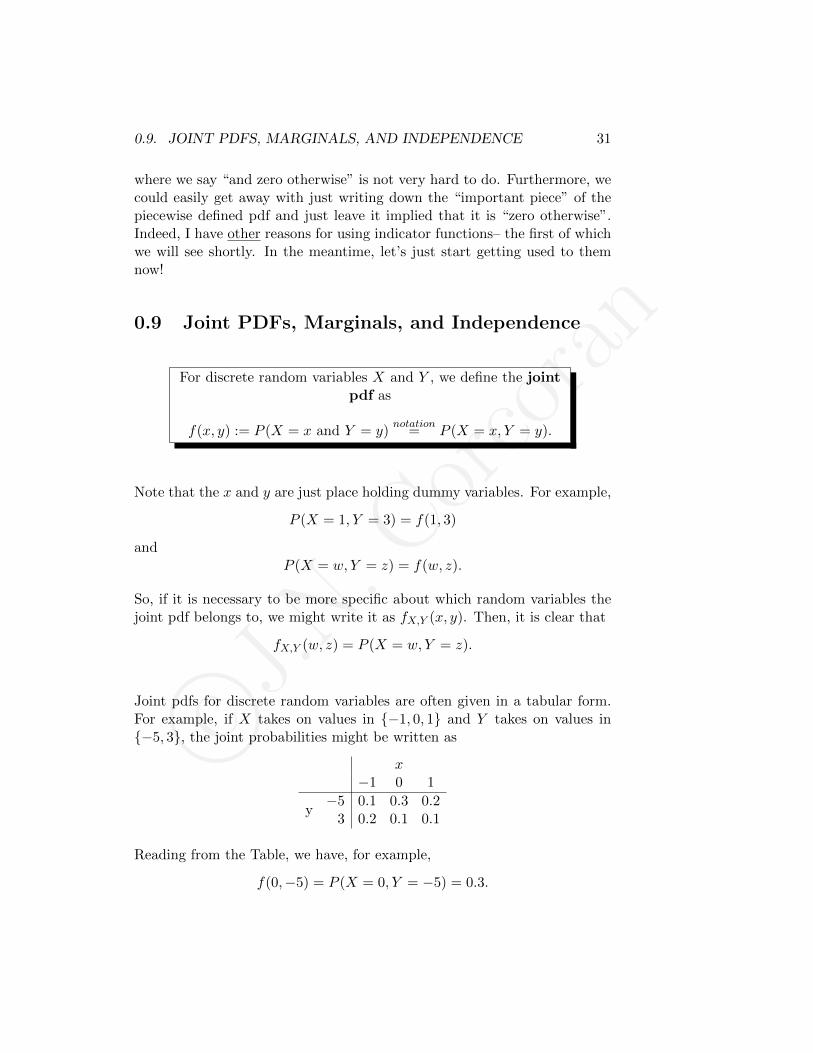
Joint pdfs for discrete random variables are often given in a tabular form.For example, if X takes on values in −1, 0, 1 and Y takes on values in−5, 3, the joint probabilities might be written as
x−1 0 1
y−5 0.1 0.3 0.2
3 0.2 0.1 0.1
Reading from the Table, we have, for example,
f(0,−5) = P (X = 0, Y = −5) = 0.3.
c©J.N.Corcoran
32 CHAPTER 0. PROBABILITY PRELIMINARIES
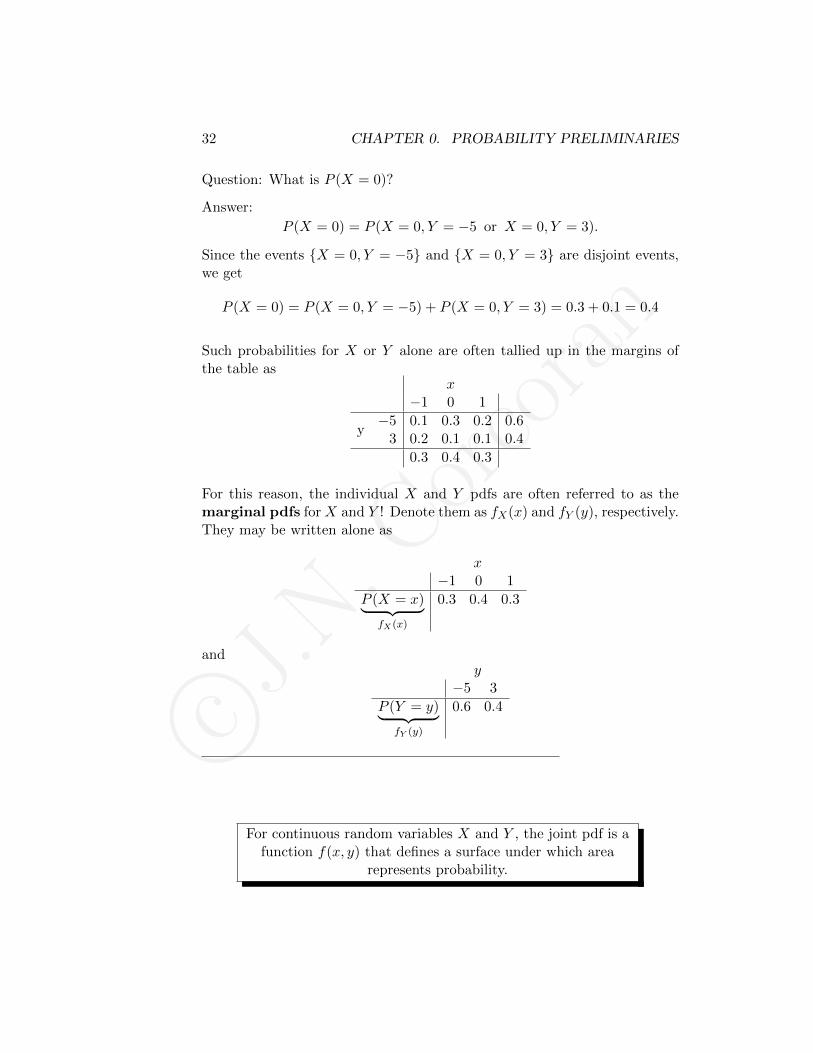
Question: What is P (X = 0)?
Answer:
P (X = 0) = P (X = 0, Y = −5 or X = 0, Y = 3).
Since the events X = 0, Y = −5 and X = 0, Y = 3 are disjoint events,we get
P (X = 0) = P (X = 0, Y = −5) + P (X = 0, Y = 3) = 0.3 + 0.1 = 0.4
Such probabilities for X or Y alone are often tallied up in the margins ofthe table as
x−1 0 1
y−5 0.1 0.3 0.2 0.6
3 0.2 0.1 0.1 0.4
0.3 0.4 0.3
For this reason, the individual X and Y pdfs are often referred to as themarginal pdfs for X and Y ! Denote them as fX(x) and fY (y), respectively.They may be written alone as
x−1 0 1
P (X = x)︸ ︷︷ ︸fX(x)
0.3 0.4 0.3
andy
−5 3
P (Y = y)︸ ︷︷ ︸fY (y)
0.6 0.4
For continuous random variables X and Y , the joint pdf is afunction f(x, y) that defines a surface under which area
represents probability.
c©J.N.Corcoran
0.9. JOINT PDFS, MARGINALS, AND INDEPENDENCE 33
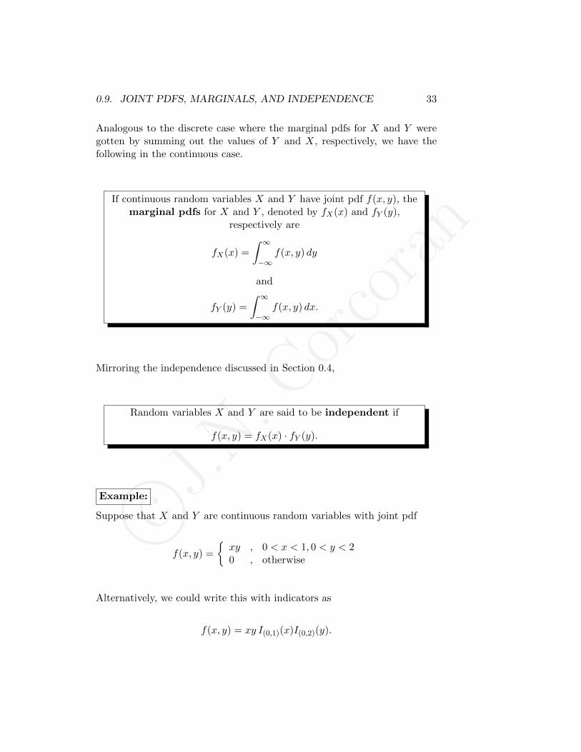
Analogous to the discrete case where the marginal pdfs for X and Y weregotten by summing out the values of Y and X, respectively, we have thefollowing in the continuous case.
If continuous random variables X and Y have joint pdf f(x, y), themarginal pdfs for X and Y , denoted by fX(x) and fY (y),
respectively are
fX(x) =
∫ ∞−∞
f(x, y) dy
and
fY (y) =
∫ ∞−∞
f(x, y) dx.
Mirroring the independence discussed in Section 0.4,
Random variables X and Y are said to be independent if
f(x, y) = fX(x) · fY (y).
Example:
Suppose that X and Y are continuous random variables with joint pdf
f(x, y) =
xy , 0 < x < 1, 0 < y < 20 , otherwise
Alternatively, we could write this with indicators as
f(x, y) = xy I(0,1)(x)I(0,2)(y).
c©J.N.Corcoran
34 CHAPTER 0. PROBABILITY PRELIMINARIES
Since this is a pdf, the total volume under this surface should be 1:∫∞−∞
∫∞−∞ f(x, y) dx dy =
∫ 20
∫ 10 xy dx dy
=∫ 2
0 y
∫ 1
0x dx︸ ︷︷ ︸
1/2
dy
= 12
∫ 20 y dy = 1
2 · 2 = 1√
Finding probabilities comes down to finding limits of integration. For ex-ample:
• P (X < 3/4, Y > 1/2) =∫ 3/4
0
∫ 21/2 f(x, y) dy dx = · · ·
• P (1/2 ≤ X ≤ 3, 1/4 ≤ Y < 1) =∫ 3
1/2
∫ 11/4 f(x, y) dy dx =
∫ 11/2
∫ 11/4 xy dy dx =
· · ·(Note the limit of integration change to the “relevant part” of the xinterval. The pdf is 0 for x = 1 to x = 3.)
• P (X ≤ Y ) =∫ 1
0
∫ x0 xy dy dx =
∫ 20
∫ 1y xy dx dy = · · ·
(Hint: Draw the rectangle where 0 ≤ x ≤ 1 and 0 ≤ y ≤ 2 and thenshade in the subregion where x ≤ y.)
The marginal pdf for X is
fX(x) =
∫ ∞−∞
f(x, y) dy =
∫ 0
−∞0 dy +
∫ 2
0xy dy +
∫ ∞2
0 dy
You obviously don’t need to write out those integrals of 0. I was just makingthe point that you should, in general, integrate over all values of y from −∞to ∞. So,
fX(x) =
∫ ∞−∞
f(x, y) dy =
∫ 2
0xy dy = 2x.
We are not finished until we write the support (the x values where it isnon-zero) of fX(x):
fX(x) = 2x 0 < x < 1.
c©J.N.Corcoran
0.9. JOINT PDFS, MARGINALS, AND INDEPENDENCE 35
The pdf is zero otherwise. We could stick on an indicator to write
fX(x) = 2x I(0,1)(x),
or we could have taken care of this automatically using indicators from thebeginning:
fX(x) =∫∞−∞ f(x, y) dy =
∫∞−∞ xy I(0,1)(x)I(0,2)(y) dy
= x I(0,1)(x)∫∞−∞ yI(0,2)(y) dy
= x I(0,1)(x)
∫ 2
0y · 1 dy︸ ︷︷ ︸
2
= 2x I(0,1)(x)
The marginal pdf for Y is
fY (y) =∫∞−∞ f(x, y) dx =
∫∞−∞ xy I(0,1)(x)I(0,2)(y) dx
= y I(0,2)(y)∫∞−∞ x I(0,1) dx
= y I(0,2)(y)
∫ 1
0x · 1 dx︸ ︷︷ ︸1/2
= 12y I(0,2)(y).
Since f(x, y) = fX(x) · fY (y), we have that X and Y are independent.
Question: If we just wanted to show independence, is it really necessary togo through the work of finding the marginal pdfs? Can’t we just say thatthe pdf f(x, y) = xy factors into an “x-part” and a “y-part even if we don’tknow quite how the constants will sort out to make marginal pdfs? (i.e.xy = x · y = 4x · (1/4)y = (1/2)x · 2y = · · ·)
Answer: We can if we use indicators!!!
c©J.N.Corcoran
36 CHAPTER 0. PROBABILITY PRELIMINARIES
For the last example, we have
f(x, y) = xy I(0,1)(x)I(0,2)(y) =(xI(0,1)(x)
)︸ ︷︷ ︸x−part
·(yI(0,2)(y)
)︸ ︷︷ ︸y−part
⇒ X and Y are independent√
Next up though is an example of a pdf that factors into an “x-part” and a“y-part but where X and Y are not independent.
Example:
Suppose that X and Y are continuous random variables with joint pdf
f(x, y) =
8xy , 0 < x < y < 10 , otherwise
For practice in finding regions of integration, let’s check that this pdf inte-grates to 1. ∫∞
−∞∫∞−∞ f(x, y) dy dx =
∫ 10
∫ x0 8xy dy dx
=∫ 1
0 8x
∫ x
0y dy︸ ︷︷ ︸
x2/2
dx
=∫ 1
0 4x3 dx = 1√
(To get these limits of integration, sketch the region where 0 < x < y < 1.It is triangular. Take any x between 0 and 1. For each such fixed x, y thenranges from 0 to x. If you want to do the integral in the opposite order,take any y between 0 and 1. For each fixed y, you’ll see that x ranges fromy to 1. So, the double integral can also be written as
∫ 10
∫ 1y 8xy dx dy.)
To find the marginal pdf, fX(x), for X, think of x as any fixed numberbetween 0 and 1. For any fixed x, y ranges from x to 1. Thus, we get
fX(x) =
∫ ∞−∞
f(x, y) dy =
∫ 1
x8xy dy = 8x
∫ 1
xy dy = 4x(1− x2).
c©J.N.Corcoran
0.9. JOINT PDFS, MARGINALS, AND INDEPENDENCE 37
This holds for 0 < x < 1. The pdf is 0 otherwise. We could just tack onan indicator in order to completely describe fX(x) or we could have usedindicators from the beginning in the joint pdf.
Note that the joint pdf could be written with indicators in two ways:
f(x, y) = 8xy I(0,1)(y) I(0,y)(x) = 8xy I(0,1)(x) I(x,1)(y).
To find the marginal pdf for X, we should use the second representationsince it has an indicator that is purely in terms of x which can be easilypulled out of an integral with respect to y:
fX(x) =∫∞−∞ f(x, y) dy =
∫∞−∞ 8xy I(0,1)(x) I(x,1)(y) dy
= 8x I(0,1)(x)∫∞−∞ y I(x,1)(y) dy
= 8x I(0,1)(x)∫ 1x y · 1 dy = 4x(1− x2) I(0,1)(x).
The marginal pdf for Y is
fY (y) =∫∞−∞ f(x, y) dx =
∫∞−∞ 8xy I(0,1)(y) I(0,y)(x) dx
= 8y I(0,1)(y)∫∞−∞ x I(0,y)(x) dx
= 8y I(0,1)(y)∫ y
0 x · 1 dy = 4y3 I(0,1)(y).
Clearly, we do not have that f(x, y) = fX(x) ·fY (y). Thus, X and Y are notindependent. We could have seen this without first finding the marginal pdfssince the indicators in the joint pdf can not be separated into an “x-part”and a “y-part”.
While the definition of independence says that X and Y are independentif the joint pdf can be factored into a product of the marginal pdfs, I triedto claim here that maybe we had independence if the joint pdf just factorsinto an x-part and a y-part and that we can leave it up to someone else tofind the marginals. This claim failed for the joint pdf f(x, y) = 8xy becausethe x and y were still tied together in the condition that 0 < x < y < 1.However, if we included this constraint in the joint pdf with indicators, weactually can show independence. We have

c©J.N.Corcoran
38 CHAPTER 0. PROBABILITY PRELIMINARIES
Random variables X and Y are independent if
f(x, y) = g(x) · h(y).
for some functions g and h, as long as we include indicators in thejoint pdf!
For the previous example, the indicator part of the joint pdf was written intwo ways,
I(0,1)(y) I(0,y)(x) and I(0,1)(x) I(x,1)(y),
but neither representation completely factors into an x-part and a y-part.
0.10 “Twisted” Indicators
Such “twisted indicators”, as in the example at the end of the previoussection, where the x and y parts are all mixed together, can sometimes besorted out. It is often helpful to see this by sketching the region where theproduct of the indicators is equal to 1.
Consider for example,
I(0,∞)(xy) · I(0,∞)(y − xy).
This product of indicators takes the value of 1 whenever both
0 < xy <∞ and 0 < y − xy <∞,
otherwise the product will be 0.
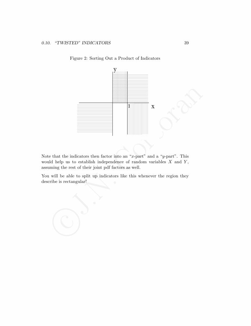
It is helpful to rewrite that second inequality as 0 < y(1 − x) < ∞. Thenwe see that it will hold when y > 0 and x < 1 OR when y < 0 and x > 1.Figure 2 shows places where I(0,∞)(xy) equals 1 using horizontal lines andplaces where I(0∞)(y − xy) is 1 using vertical lines.
Both indicators (and hence their product) is 1 on the region where 0 < x < 1and 0 < y <∞. Thus, we have that
I(0,∞)(xy) · I(0∞)(y − xy) = I(0,1)(x) · I(0,∞)(y).
c©J.N.Corcoran
0.10. “TWISTED” INDICATORS 39
Figure 2: Sorting Out a Product of Indicators
Note that the indicators then factor into an “x-part” and a “y-part”. Thiswould help us to establish independence of random variables X and Y ,assuming the rest of their joint pdf factors as well.
You will be able to split up indicators like this whenever the region theydescribe is rectangular!

c©J.N.Corcoran
40 CHAPTER 0. PROBABILITY PRELIMINARIES

c©J.N.Corcoran
Chapter 1
MathStat Preliminaries:Four Important Tools forMathematical Statistics
1.1 Wait. Where are we going?
Recall the exponential distribution introduced in Section 0.5.3. If X ∼exp(rate = λ), then X has the pdf
f(x) =
λe−λx , x ≥ 00 , x < 0
which looks like this
41
c©J.N.Corcoran
42CHAPTER 1. MATHSTAT PRELIMINARIES: FOUR IMPORTANT TOOLS FORMATHEMATICAL STATISTICS
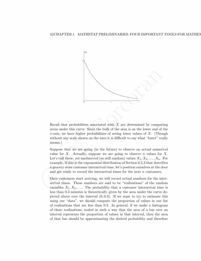
x
f(x)
λ
0
Recall that probabilities associated with X are determined by computingareas under this curve. Since the bulk of the area is on the lower end of thex-axis, we have higher probabilities of seeing lower values of X. (Thoughwithout any scale shown on the axes it is difficult to say what “lower” reallymeans.)
Suppose that we are going (in the future) to observe an actual numericalvalue for X. Actually, suppose we are going to observe n values for X.Let’s call these, yet unobserved (so still random) values X1, X2, . . . , Xn. Forexample, if this is the exponential distribution of Section 0.5.3 that describesa grocery store customer interarrival time, let’s position ourselves at the doorand get ready to record the interarrival times for the next n customers.
Once customers start arriving, we will record actual numbers for the inter-arrival times. These numbers are said to be “realizations” of the randomvariables X1, X2, . . .. The probability that a customer interarrival time isless than 0.3 minutes is theoretically given by the area under the curve de-picted above over the interval (0, 0.3). If we want to try to estimate thisusing our “data”, we should compute the proportion of values in our listof realizations that are less than 0.3. In general, if we make a histogramof these realizations, scaled in such a way that the area of a bar over aninterval represents the proportion of values in that interval, then the areaof that bar should be approximating the desired probability and therefore

c©J.N.Corcoran
1.1. WAIT. WHERE ARE WE GOING? 43
should be approximating the true area under the pdf.
Here is such a histogram of 10 realizations of X where X ∼ exp(rate = 15.2).
Histogram of 10 Interarrival Times
x
Density
0.00 0.02 0.04 0.06 0.08 0.10 0.12 0.14
05
10
15
20
That doesn’t look much like the exponential pdf. However, with moredata/realizations, we get the following.
Histogram of 10,000 Interarrival Times
y
Density
0.0 0.1 0.2 0.3 0.4 0.5 0.6 0.7
02
46
810
Overlaying the pdf f(x) = 15.2e−15.2x for x > 0 gives us a pretty good fit!

c©J.N.Corcoran
44CHAPTER 1. MATHSTAT PRELIMINARIES: FOUR IMPORTANT TOOLS FORMATHEMATICAL STATISTICS
Histogram of 10,000 Interarrival Times
y
Density
0.0 0.1 0.2 0.3 0.4 0.5 0.6 0.7
02
46
810
Suppose now that we only have those 10,000 data points and the belief thatthey came from an exponential distribution, but we do not know the valueof λ. How would you estimate λ?
We could use the fact that 1/λ is the expected value (mean) for the expo-nential distribution. Recall that this is a probability weighted average. Wecould just average the 10,000 values we sampled/recorded. They alreadyhave their “probability weights” built-in in the way they were generated,with, for example, lower values coming out more often. This average isknown as a sample mean and is denoted by x. If we have yet to recordnumerical values but are planning on recording 10,000 of them and averag-ing them, we would denote the sample mean with the X, which is anotherrandom variable.
Using the observation above about the expected value or “distribution mean”and the sample mean, one plan for estimating λ is to think that
1/λ ≈ X
and to solve for λ. This gives
λ ≈ 1/X.
So, once we get the data and compute the sample mean, we could flip itover and use that to estimate the unknown λ.
An alternative way to estimate the unknown λ might be to notice that itis the y-intercept on the graph of the pdf. Could we make a more refined
c©J.N.Corcoran
1.2. IMPORTANT TOOL I: FINDING DISTRIBUTIONS OF TRANSFORMATIONS OF RANDOMVARIABLES45
histogram with really thin bars and try to estimate λ using the height ofthe first bar? In the last histogram shown above, the first bar is quite a bitlower than 15.2. If we made each bar half as wide, the first bar would likelyshoot up much higher. What if we made them one quarter as wide? Surelywe couldn’t keep shrinking them because we only have a finite amount ofdata and so we would only have a very small number of values in very smallintervals. Indeed, the first bar height/area might shrink to zero!
It seems that the “y-intercept idea” is somehow not as “solid” as the samplemean idea. A large part of mathematical statistics is coming up with waysto estimate parameters after we first quantify what is meant by a “goodestimator” and what is meant by a “better estimator”. Before we get started,we are going to need some more tools under our belts.
1.2 Important Tool I: Finding Distributions of Trans-formations of Random Variables
1.2.1 The Discrete Case and the Binomial Distribution
Let me use this opportunity first to introduce (or remind you of) anotherdistribution.
Consider a sequence of n independent trials of an experiment where eachtrial can result in either “successes” (S) or “failure” (F ). Suppose that theprobability of success remains the same from trial to trial. Call it p where0 ≤ p ≤ 1.
Let
X = # of successes in n trials.
While it looks similar, this is different from the geometric random variableintroduced in Chapter 0. There, we continued trials until the first success.Here, we will have a n (a fixed number) of trials and count up all thesuccesses.
In this case, X is said to have a binomial distribution with parameters nand p.
We write
X ∼ bin(n, p).
c©J.N.Corcoran
46CHAPTER 1. MATHSTAT PRELIMINARIES: FOUR IMPORTANT TOOLS FORMATHEMATICAL STATISTICS
As the number of successes in n trials, X can take on values in 0, 1, 2, . . . , n.
The pdf is
f(x) = P (X = x) = P (SSFSF . . . F or SFSFS . . . S or . . .)
where each listed configuration of outcomes includes exactly x S’s and ex-actly n− x F ’s. Since the outcomes are disjoint, we get
f(x) = P (X = x) = P (SSFSF . . . F ) + P (SFSFS . . . S) + · · · (1.1)
Since the trials are independent,
P (SSFSF . . . F ) = p · p · (1− p) · s · (1− p) · · · (1− p) = px(1− p)n−x.
In fact, every term in (1.1) gives that same probability! So,
f(x) = P (X = x) = c · px(1− p)n−x
where c is the number of terms in (1.1).
How many ways are there to write down sequences of n S’s and F ’s withexactly x S’s? We need to choose x slots out of n in which to put the S’s.There are (
nx
)=
n!
x!(n− x)!
different ways to do this. Thus,
c =
(nx
).
So, we have seen that X ∼ bin(n, p) means that X has pdf
f(x) = P (X = x) =
(nx
)px(1− p)n−x I0,1,...,n(x) (1.2)
Check out the binomial distribution in the distribution tables in AppendixA.
c©J.N.Corcoran
1.2. IMPORTANT TOOL I: FINDING DISTRIBUTIONS OF TRANSFORMATIONS OF RANDOMVARIABLES47
Now for a transformation...
Suppose that X ∼ bin(n, p). Find the distribution (Name it!) for therandom variable Y := n−X.
The answer to this one is quite “guessable”, but let’s go through the motionsanyway since this will not always be the case.
The pdf for Y is
fY (y) = P (Y = y) =?
What choice do we have but to use the fact that Y = n − X? We don’tknow anything else about Y . Just do the problem and don’t worry about a“formula” for transforming the pdf! So,
fY (y) = P (Y = y) = P (n−X = y)
Now, we do know how to compute probabilities of the form P (X =?), so,solve for X here to get
fY (y) = P (Y = y) = P (n−X = y) = P (X = n− y)
and use the pdf for X, plugging in n− y where there were x′s in (1.2):
fY (y) = P (Y = y) = P (n−X = y) = P (X = n− y)
(1.2)=
(n
n− y
)pn−y(1− p)n−(n−y) I0,1,...,n(n− y)
=
(n
n− y
)pn−y(1− p)y I0,1,...,n(y)
I simplified the exponent n−(n−y) for obvious reasons, but I also simplifiedthe indicator for two reasons.
1. It’s good form. After all, you are reporting a function of y. Why wouldyou say “This holds for n− y in the set 0, 1, 2, . . . n.” as opposed tosaying what y alone can be?
2. It will make it easier to recognize the distribution of Y .
c©J.N.Corcoran
48CHAPTER 1. MATHSTAT PRELIMINARIES: FOUR IMPORTANT TOOLS FORMATHEMATICAL STATISTICS
To simplify the indicator I0,1,...,n(n−y), note that is is equal to 1 whenever
n− y = 0, 1, 2, . . . , n.
But,n− y = 0 ⇒ y = n,
n− y = 1 ⇒ y = n− 1,
...
n− y = n ⇒ y = 0.
So, y takes on values in 0, 1, . . . , n.
(Another note on good versus bad “form”: order is unimportant for listingelements in a set, but, in my opinion, to say that “y takes on values inn, n − 1, . . . , 0” is kind of weird and, also in my opinion, shows that youare just “plugging and chugging” through steps of a problem without reallythinking about what you’re doing.)
In summary,I0,1,...,n(n− y) = I0,1,...,n(y),
so the pdf for Y is
fY (y) =
(n
n− y
)pn−y(1− p)n−(n−y) I0,1,...,n(y).
When trying to match this up to a distribution in our table of distributions,you will see only two discrete distributions with this type of indicator. Oneis the discrete uniform distribution whose pdf does not at all resemble thispdf and the other is the binomial distribution. Note that(
ny
)=
n!
y!(n− y)!=
n!
(n− y)!y!=
n!
(n− y)!(n− (n− y))!=
(n
n− y
).
Moving the p’s around, we can write the pdf for Y as
fY (y) =
(ny
)(1− p)ypn−y I0,1,...,n(y)
to see thatY ∼ bin(n, 1− p).
Surprised? Probably not. If X is the number of successes in n trials, thenY = n − X is the number of failures. Relabeling successes as failures, the“success probability” is now 1− p.
c©J.N.Corcoran
1.2. IMPORTANT TOOL I: FINDING DISTRIBUTIONS OF TRANSFORMATIONS OF RANDOMVARIABLES49
Probability density functions of transformations of random variables do notalways turn out to be those of nice “named” distributions. When I ask youto “Find the distribution.”, I will mean a named distribution, otherwise Iwould have just asked you to “Find the pdf.” To be more clear, I will follow“Find the distribution.” with “(Name it!)”
1.2.2 The Continuous Case and the Gamma Distribution
In the discrete case, we didn’t need some sort of general formula for makinga transformation of pdfs from one random variable to another. Since pdfswere probabilities, it was easiest just to write out what we want and whatwe know and to go! In the continuous case, the pdf no longer representsprobability (i.e. f(x) 6= P (X = x)), so the approach from the discrete casewill not make sense. The good news though is that we do have probabilitiesin the cdfs! So, the plan will be to find
FY (y) = P (Y ≤ y) = · · ·
and then in the end to find the pdf for Y using the fact that
fY (y) =d
dyFY (y).
Suppose that X has pdf fX(x) and cdf FX(x).
Suppose that Y is defined as Y = g(X).
We will assume that g is invertible. (If it is not, it doesn’t mean we are outof luck, it just means that this approach and the formula we are about toderive won’t work.)
Note that
1. g invertible ⇒ g is either strictly increasing or strictly decreasing.
2. If g is increasing (alternatively decreasing) the g−1 is also increasing(alternatively decreasing).
c©J.N.Corcoran
50CHAPTER 1. MATHSTAT PRELIMINARIES: FOUR IMPORTANT TOOLS FORMATHEMATICAL STATISTICS
To see that second point in the increasing case, note that g increasingmeans that x1 ≤ x2 implies that g(x1) ≤ g(x2) and that x1 ≥ x2
implies that g(x1) ≥ g(x2). (It might help to draw a picture.)
We want to show that g−1 is also increasing. Suppose that x1 ≤ x2.We want to show that g−1(x1) ≤ g−1(x2). Suppose (incorrectly) that
g−1(x1) ≥ g−1(x2).
We are going to take g of both sides. Since g is increasing, it preservesthe order of the inequality:
g(g−1(x1)) ≥ g(g−1(x2)).
Canceling g and g−1 gives
x1 ≥ x2.
This contradicts the original assumption that x1 ≤ x2. Thus, we musthave that g−1(x1) ≤ g−1(x2) and thus that g−1 is increasing.
We are ready to find an expression for the cdf, and then the pdf, for Y .
Case One: g is increasing.
FY (y) = P (Y ≤ y) = P (g(X) ≤ y)
Applying g−1 to both sides of that inequality, and using the fact that gincreasing ⇒ g−1 increasing ⇒ g−1 applied to both sides of an inequalitywill preserve the order, we get
FY (y) = P (Y ≤ y) = P (g(X) ≤ y)
= P (g−1(g(X)) ≤ g−1(y))
= P (X ≤ g−1(y))
= FX(g−1(y))
Thus, the pdf for Y is
fY (y) =d
dyFY (y) =
d
dyFX(g−1(y))
chain rule= fX(g−1(y)) · d
dyg−1(y)

c©J.N.Corcoran
1.2. IMPORTANT TOOL I: FINDING DISTRIBUTIONS OF TRANSFORMATIONS OF RANDOMVARIABLES51
Note that g−1 increasing implies that that derivative is greater than zero.
Case Two: g is decreasing.
FY (y) = P (Y ≤ y) = P (g(X) ≤ y)
Applying g−1 to both sides of that inequality, and using the fact that gdecreasing ⇒ g−1 decreasing ⇒ g−1 applied to both sides of an inequalitywill flip the inequality, we get
FY (y) = P (Y ≤ y) = P (g(X) ≤ y)
= P (g−1(g(X)) ≥ g−1(y))
= P (X ≥ g−1(y))
= 1− P (X < g−1(y)
contin= 1− P (X ≤ g−1(y))
= 1− FX(g−1(y))
Thus, the pdf for Y is
fY (y) = ddyFY (y) = d
dy [1− FX(g−1(y))]
chain rule= [0− fX(g−1(y)) · ddyg
−1(y)]
= −fX(g−1(y)) · ddyg−1(y)
Note that, since g−1 is decreasing (actually strictly so), we have ddyg−1(y) <
0, so, no, we did not end up with a negative pdf! Furthermore, note that− ddyg−1(y) is positive and equal to | ddyg
−1(y)|.
In the previous increasing case, ddyg−1(y) is positive and equal to | ddyg
−1(y)|.
In summary, we can write both the increasing and decreasing cases togetheras follows.

c©J.N.Corcoran
52CHAPTER 1. MATHSTAT PRELIMINARIES: FOUR IMPORTANT TOOLS FORMATHEMATICAL STATISTICS
Let X be a continuous random variable with pdf fx. Let Y be arandom variable defined by Y = g(X) where g is invertible (anddifferentiable). Then the pdf for Y can be computed as
fY (y) = fX(g−1(y)) ·∣∣∣∣ ddyg−1(y)
∣∣∣∣ .
Example:
Let X have a “gamma distribution with parameters α and β” We writeX ∼ Γ(α, β). This means that X is a continuous random variable with pdf
fX(x) =1
Γ(α)βαxα−1e−βx I(0,∞)(x)
for some parameters α > 0 and β > 0.
Notes:
1. We are using the X subscript on the pdf because we will have multiplepdfs in this problem– one for X and one for a new random variable Y .
2. For some people/books, X ∼ Γ(α, β) means that X has pdf
fX(x) =1
Γ(α)(1/β)αxα−1e−x/β I(0,∞)(x).
Here, α and β are known as the “shape” and “scale” parameters,respectively.
For our form of the gamma pdf, β is known as the “inverse scaleparameter”.
3. The pdf involves the “gamma function”, Γ(α). It is just a constant.We will define it after finishing this example. The constant Γ(α) shouldnot be confused with Γ(α, β) (two arguments) which is the name of adistribution.
Let Y = 5X. Find the distribution of Y . (Name it!)
c©J.N.Corcoran
1.2. IMPORTANT TOOL I: FINDING DISTRIBUTIONS OF TRANSFORMATIONS OF RANDOMVARIABLES53
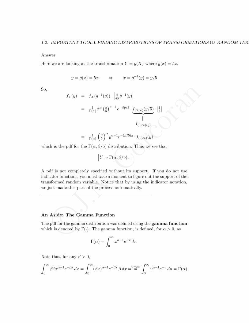
Answer:
Here we are looking at the transformation Y = g(X) where g(x) = 5x.
y = g(x) = 5x ⇒ x = g−1(y) = y/5
So,
fY (y) = fX(g−1(y)) ·∣∣∣ ddyg−1(y)
∣∣∣= 1
Γ(α)βα(y
5
)α−1e−βy/5 · I(0,∞)(y/5)︸ ︷︷ ︸
||I(0,∞)(y)
·∣∣1
5
∣∣
= 1Γ(α)
(β5
)αyα−1e−(β/5)y · I(0,∞)(y)
which is the pdf for the Γ(α, β/5) distribution. Thus we see that
Y ∼ Γ(α, β/5).
A pdf is not completely specified without its support. If you do not useindicator functions, you must take a moment to figure out the support of thetransformed random variable. Notice that by using the indicator notation,we just made this part of the process automatically.
An Aside: The Gamma Function
The pdf for the gamma distribution was defined using the gamma functionwhich is denoted by Γ(·). The gamma function, is defined, for α > 0, as
Γ(α) =
∫ ∞0
xα−1e−x dx.
Note that, for any β > 0,∫ ∞0
βαxα−1e−βx dx =
∫ ∞0
(βx)α−1e−βx β dx =u=βx
=
∫ ∞0
uα−1e−u du = Γ(α)
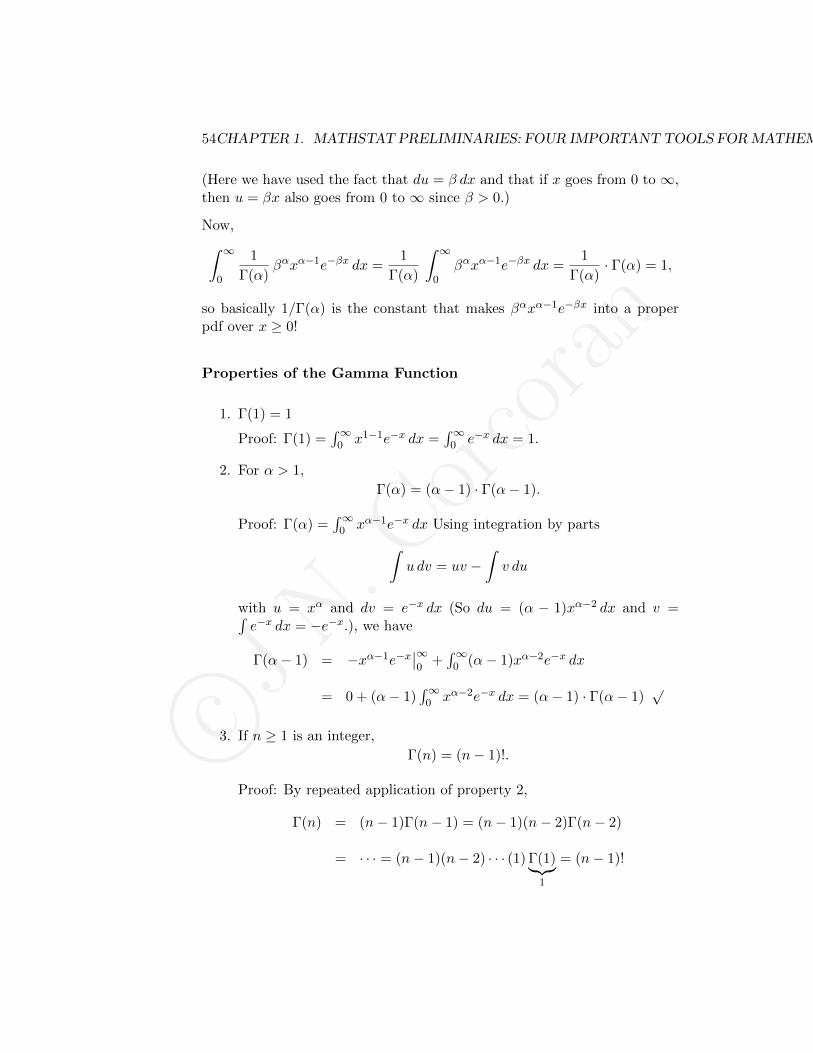
c©J.N.Corcoran
54CHAPTER 1. MATHSTAT PRELIMINARIES: FOUR IMPORTANT TOOLS FORMATHEMATICAL STATISTICS
(Here we have used the fact that du = β dx and that if x goes from 0 to ∞,then u = βx also goes from 0 to ∞ since β > 0.)
Now,∫ ∞0
1
Γ(α)βαxα−1e−βx dx =
1
Γ(α)
∫ ∞0
βαxα−1e−βx dx =1
Γ(α)· Γ(α) = 1,
so basically 1/Γ(α) is the constant that makes βαxα−1e−βx into a properpdf over x ≥ 0!
Properties of the Gamma Function
1. Γ(1) = 1
Proof: Γ(1) =∫∞
0 x1−1e−x dx =∫∞
0 e−x dx = 1.
2. For α > 1,
Γ(α) = (α− 1) · Γ(α− 1).
Proof: Γ(α) =∫∞
0 xα−1e−x dx Using integration by parts∫u dv = uv −
∫v du
with u = xα and dv = e−x dx (So du = (α − 1)xα−2 dx and v =∫e−x dx = −e−x.), we have
Γ(α− 1) = −xα−1e−x∣∣∞0
+∫∞
0 (α− 1)xα−2e−x dx
= 0 + (α− 1)∫∞
0 xα−2e−x dx = (α− 1) · Γ(α− 1)√
3. If n ≥ 1 is an integer,
Γ(n) = (n− 1)!.
Proof: By repeated application of property 2,
Γ(n) = (n− 1)Γ(n− 1) = (n− 1)(n− 2)Γ(n− 2)
= · · · = (n− 1)(n− 2) · · · (1) Γ(1)︸︷︷︸1
= (n− 1)!
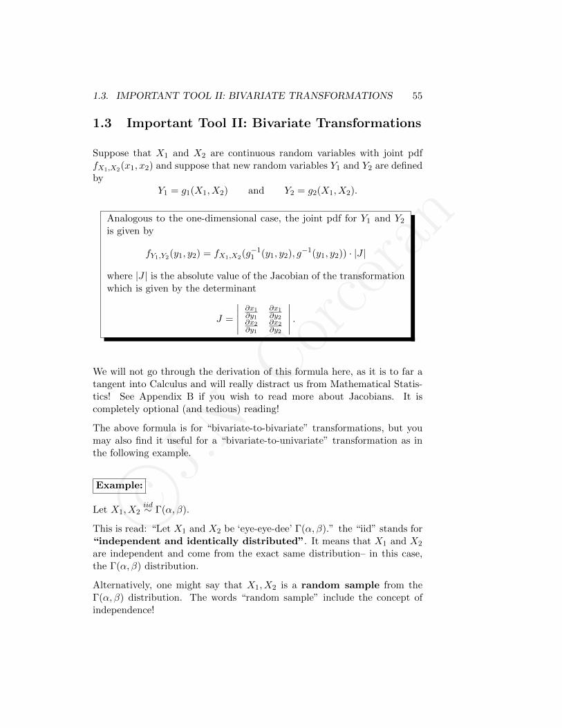
c©J.N.Corcoran
1.3. IMPORTANT TOOL II: BIVARIATE TRANSFORMATIONS 55
1.3 Important Tool II: Bivariate Transformations
Suppose that X1 and X2 are continuous random variables with joint pdffX1,X2(x1, x2) and suppose that new random variables Y1 and Y2 are definedby
Y1 = g1(X1, X2) and Y2 = g2(X1, X2).
Analogous to the one-dimensional case, the joint pdf for Y1 and Y2
is given by
fY1,Y2(y1, y2) = fX1,X2(g−11 (y1, y2), g−1(y1, y2)) · |J |
where |J | is the absolute value of the Jacobian of the transformationwhich is given by the determinant
J =
∣∣∣∣∣ ∂x1∂y1
∂x1∂y2
∂x2∂y1
∂x2∂y2
∣∣∣∣∣ .
We will not go through the derivation of this formula here, as it is to far atangent into Calculus and will really distract us from Mathematical Statis-tics! See Appendix B if you wish to read more about Jacobians. It iscompletely optional (and tedious) reading!
The above formula is for “bivariate-to-bivariate” transformations, but youmay also find it useful for a “bivariate-to-univariate” transformation as inthe following example.
Example:
Let X1, X2iid∼ Γ(α, β).
This is read: “Let X1 and X2 be ‘eye-eye-dee’ Γ(α, β).” the “iid” stands for“independent and identically distributed”. It means that X1 and X2
are independent and come from the exact same distribution– in this case,the Γ(α, β) distribution.
Alternatively, one might say that X1, X2 is a random sample from theΓ(α, β) distribution. The words “random sample” include the concept ofindependence!
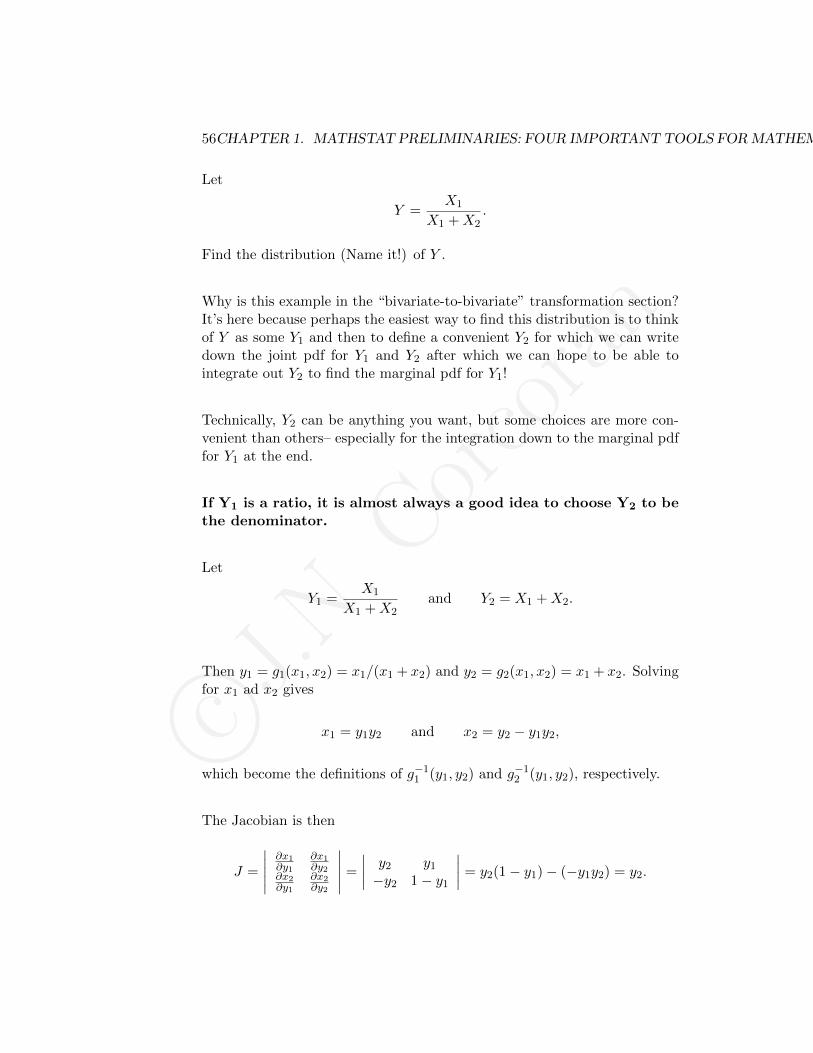
c©J.N.Corcoran
56CHAPTER 1. MATHSTAT PRELIMINARIES: FOUR IMPORTANT TOOLS FORMATHEMATICAL STATISTICS
Let
Y =X1
X1 +X2.
Find the distribution (Name it!) of Y .
Why is this example in the “bivariate-to-bivariate” transformation section?It’s here because perhaps the easiest way to find this distribution is to thinkof Y as some Y1 and then to define a convenient Y2 for which we can writedown the joint pdf for Y1 and Y2 after which we can hope to be able tointegrate out Y2 to find the marginal pdf for Y1!
Technically, Y2 can be anything you want, but some choices are more con-venient than others– especially for the integration down to the marginal pdffor Y1 at the end.
If Y1 is a ratio, it is almost always a good idea to choose Y2 to bethe denominator.
Let
Y1 =X1
X1 +X2and Y2 = X1 +X2.
Then y1 = g1(x1, x2) = x1/(x1 + x2) and y2 = g2(x1, x2) = x1 + x2. Solvingfor x1 ad x2 gives
x1 = y1y2 and x2 = y2 − y1y2,
which become the definitions of g−11 (y1, y2) and g−1
2 (y1, y2), respectively.
The Jacobian is then
J =
∣∣∣∣∣ ∂x1∂y1
∂x1∂y2
∂x2∂y1
∂x2∂y2
∣∣∣∣∣ =
∣∣∣∣ y2 y1
−y2 1− y1
∣∣∣∣ = y2(1− y1)− (−y1y2) = y2.
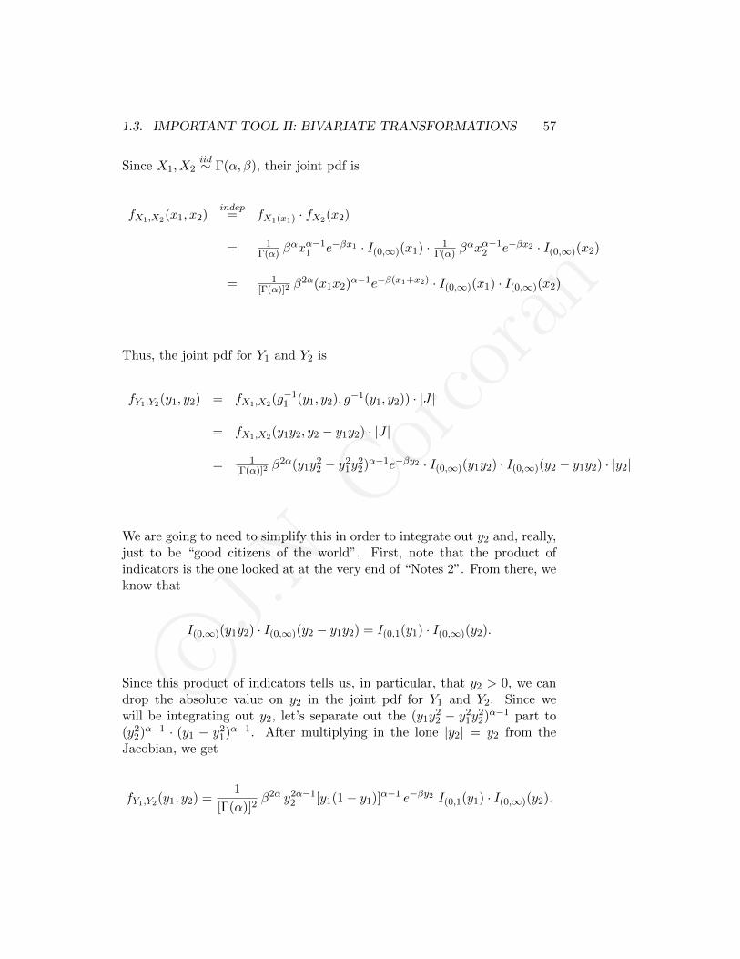
c©J.N.Corcoran
1.3. IMPORTANT TOOL II: BIVARIATE TRANSFORMATIONS 57
Since X1, X2iid∼ Γ(α, β), their joint pdf is
fX1,X2(x1, x2)indep= fX1(x1) · fX2(x2)
= 1Γ(α) β
αxα−11 e−βx1 · I(0,∞)(x1) · 1
Γ(α) βαxα−1
2 e−βx2 · I(0,∞)(x2)
= 1[Γ(α)]2
β2α(x1x2)α−1e−β(x1+x2) · I(0,∞)(x1) · I(0,∞)(x2)
Thus, the joint pdf for Y1 and Y2 is
fY1,Y2(y1, y2) = fX1,X2(g−11 (y1, y2), g−1(y1, y2)) · |J |
= fX1,X2(y1y2, y2 − y1y2) · |J |
= 1[Γ(α)]2
β2α(y1y22 − y2
1y22)α−1e−βy2 · I(0,∞)(y1y2) · I(0,∞)(y2 − y1y2) · |y2|
We are going to need to simplify this in order to integrate out y2 and, really,just to be “good citizens of the world”. First, note that the product ofindicators is the one looked at at the very end of “Notes 2”. From there, weknow that
I(0,∞)(y1y2) · I(0,∞)(y2 − y1y2) = I(0,1(y1) · I(0,∞)(y2).
Since this product of indicators tells us, in particular, that y2 > 0, we candrop the absolute value on y2 in the joint pdf for Y1 and Y2. Since wewill be integrating out y2, let’s separate out the (y1y
22 − y2
1y22)α−1 part to
(y22)α−1 · (y1 − y2
1)α−1. After multiplying in the lone |y2| = y2 from theJacobian, we get
fY1,Y2(y1, y2) =1
[Γ(α)]2β2α y2α−1
2 [y1(1− y1)]α−1 e−βy2 I(0,1(y1) · I(0,∞)(y2).

c©J.N.Corcoran
58CHAPTER 1. MATHSTAT PRELIMINARIES: FOUR IMPORTANT TOOLS FORMATHEMATICAL STATISTICS
Now for the marginal...
fY1(y1) =∫∞−∞ fY1,Y2(y1, y2) dy2
= 1[Γ(α)]2
β2α [y1(1− y1)]α−1 I(0,1)(y1)∫∞
0 y2α−12 e−βy2︸ ︷︷ ︸
like a
Γ(2α, β)pdf
dy2
= Γ(2α)[Γ(α)]2
[y1(1− y1)]α−1 I(0,1)(y1)∫∞
0
1
Γ(2α)β2α y2α−1
2 e−βy2︸ ︷︷ ︸actually a Γ(2α, β)pdf, so integrates
to 1
dy2
= Γ(2α)[Γ(α)]2
[y1(1− y1)]α−1 I(0,1)(y1)
If you look in your table of distributions (continuous side) you’ll see thatthere are only two possibilities for this distribution based on the indicator.One is the uniform distribution on the interval (0, 1). That is a flat linedistribution with height 1 on the interval. It has pdf f(x) = I(0,1)(x). Themarginal pdf we have computed is a little more complicated than that.
The second distribution on a finite interval, and, in particular on the intervalfrom (0, 1), is called the “Beta distribution”. This distribution has twoparameters, α and β, and is given in the table as having pdf
f(x) =1
B(a, b)xa−1(1− x)b−1 dx.
We would write X ∼ Beta(a, b).
Our marginal pdf for Y1 looks a lot like this one (written as a function ofy1). But... what about our “Γ stuff” versus this thing we have yet to definewritten as B(a, b)? (This is known as the “Beta function”.)
The “Γ stuff” and the “Beta stuff” are just constants. They have to matchin order for these both to be pdfs! For example, we know that f(x) =2e−2x I(0,1)(x) is a pdf. It’s the exponential with rate 2 pdf. From this, we

c©J.N.Corcoran
1.3. IMPORTANT TOOL II: BIVARIATE TRANSFORMATIONS 59
know that the function 5e−2x I(0,∞)(x) is not a pdf! It can’t integrate to 1if 2e−2x I(0,∞)(x) integrates to 1. In fact,∫ ∞
05e−2x dx =
5
2
∫ ∞0
2e−2x dx =5
2· 1 =
5
2.
If you followed our transformational procedures correctly, you are guaran-teed to get a pdf in the end. Thus, our pdf
fY1(y1) =Γ(2α)
[Γ(α)]2[y1(1− y1)]α−1 I(0,1)(y1)
must be the pdf for the Beta distribution with parameters a = α andb = α. We write
Y ∼ Beta(α, α).
1.3.1 The Beta Distribution
The Beta distribution was defined at the end of the previous section. (Infact, the only reason I am making this short extra section is so that you willsee “Beta distribution” in the table of contents!)
This distribution is a nice flexible distribution that is suitable to modelthings that are supposed to be between 0 and 1. (If I didn’t just need to getthese notes posted right now, I would make some graphs. Note that whena = b = 1, it is the uniform distribution on (0, 1). For a, b < 1, it has a“u-shape”. For a, b > 1 it is a unimodal distribution that is tied down to 0at both endpoints and various vales of a and b in this range can move the“lump” around to wherever you want it!
Just for the record, the Beta function is defined, for a, b > 0, as
B(a, b) =
∫ 1
0xa−1 (1− x)b−1 dx.
It is possible, though not that fun, to show the relationship
B(a, b) =Γ(a)Γ(b)
Γ(a+ b).
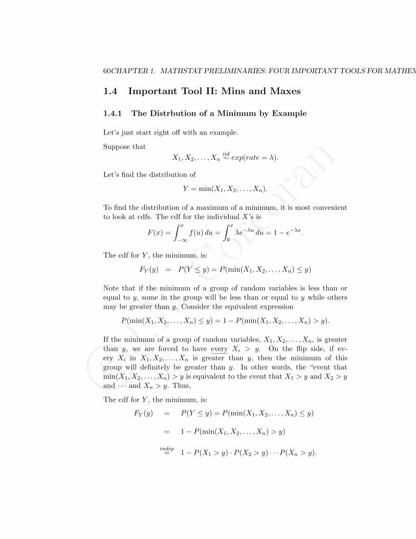
c©J.N.Corcoran
60CHAPTER 1. MATHSTAT PRELIMINARIES: FOUR IMPORTANT TOOLS FORMATHEMATICAL STATISTICS
1.4 Important Tool II: Mins and Maxes
1.4.1 The Distrbution of a Minimum by Example
Let’s just start right off with an example.
Suppose that
X1, X2, . . . , Xniid∼ exp(rate = λ).
Let’s find the distribution of
Y = min(X1, X2, . . . , Xn).
To find the distribution of a maximum of a minimum, it is most convenientto look at cdfs. The cdf for the individual X’s is
F (x) =
∫ x
−∞f(u) du =
∫ x
0λe−λu du = 1− e−λx.
The cdf for Y , the minimum, is:
FY (y) = P (Y ≤ y) = P (min(X1, X2, . . . , Xn) ≤ y)
Note that if the minimum of a group of random variables is less than orequal to y, some in the group will be less than or equal to y while othersmay be greater than y. Consider the equivalent expression
P (min(X1, X2, . . . , Xn) ≤ y) = 1− P (min(X1, X2, . . . , Xn) > y).
If the minimum of a group of random variables, X1, X2, . . . , Xn, is greaterthan y, we are forced to have every Xi > y. On the flip side, if ev-ery Xi in X1, X2, . . . , Xn is greater than y, then the minimum of thisgroup will definitely be greater than y. In other words, the “event thatmin(X1, X2, . . . , Xn) > y is equivalent to the event that X1 > y and X2 > yand · · · and Xn > y. Thus,
The cdf for Y , the minimum, is:
FY (y) = P (Y ≤ y) = P (min(X1, X2, . . . , Xn) ≤ y)
= 1− P (min(X1, X2, . . . , Xn) > y)
indep= 1− P (X1 > y) · P (X2 > y) · · ·P (Xn > y).
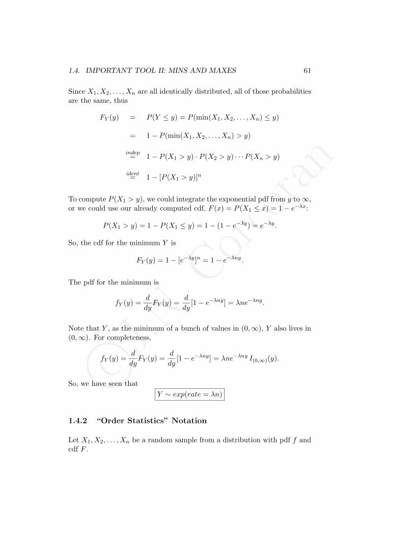
c©J.N.Corcoran
1.4. IMPORTANT TOOL II: MINS AND MAXES 61
Since X1, X2, . . . , Xn are all identically distributed, all of those probabilitiesare the same, thus
FY (y) = P (Y ≤ y) = P (min(X1, X2, . . . , Xn) ≤ y)
= 1− P (min(X1, X2, . . . , Xn) > y)
indep= 1− P (X1 > y) · P (X2 > y) · · ·P (Xn > y)
ident= 1− [P (X1 > y)]n
To compute P (X1 > y), we could integrate the exponential pdf from y to∞,or we could use our already computed cdf, F (x) = P (X1 ≤ x) = 1− e−λx:
P (X1 > y) = 1− P (X1 ≤ y) = 1− (1− e−λy) = e−λy.
So, the cdf for the minimum Y is
FY (y) = 1− [e−λy]n = 1− e−λny.
The pdf for the minimum is
fY (y) =d
dyFY (y) =
d
dy[1− e−λny] = λne−λny.
Note that Y , as the minimum of a bunch of values in (0,∞), Y also lives in(0,∞). For completeness,
fY (y) =d
dyFY (y) =
d
dy[1− e−λny] = λne−λny I(0,∞)(y).
So, we have seen that
Y ∼ exp(rate = λn)
1.4.2 “Order Statistics” Notation
Let X1, X2, . . . , Xn be a random sample from a distribution with pdf f andcdf F .

c©J.N.Corcoran
62CHAPTER 1. MATHSTAT PRELIMINARIES: FOUR IMPORTANT TOOLS FORMATHEMATICAL STATISTICS
Notation: Define
X(1) = min(X1, X2, . . . , Xn)
X(2) = the second smallest of the X’s...
...X(n) = max(X1, X2, . . . , X(n))
The X(1), X(2), . . . , X(n) form a new collection of random variables knownas the order statistics of the original sample. (Another commonly usednotation for the order statistics is X1:n, X2:n, . . . , Xn:n.)
We will discuss order statistics in general in Section ??. For now, we willjust focus on minimums and maximums.
1.4.3 PDFs for Minimums and Maximums
In this section, we will derive the pdf and cdf for minimums and maximumsfor a random sample from a continuous distribution only. We’ll work outthe discrete case in the future as needed. (It’s a bit messy!)
Minimums:
In the example of Section 1.4.1, we have already basically derived an ex-pression for the pdf of the minimum in terms of f and F , the pdf and cdfrespectively for the original random variables.
FX(1)(x) = P (X(1) ≤ x) = P (min(X1, X2, . . . , Xn) ≤ x)
= 1− P (min(X1, X2, . . . , Xn) > x)
indep= 1− P (X1 > x) · P (X2 > x) · · ·P (Xn > x)
ident= 1− [P (X1 > x)]n
= 1− [1− F (x)]n
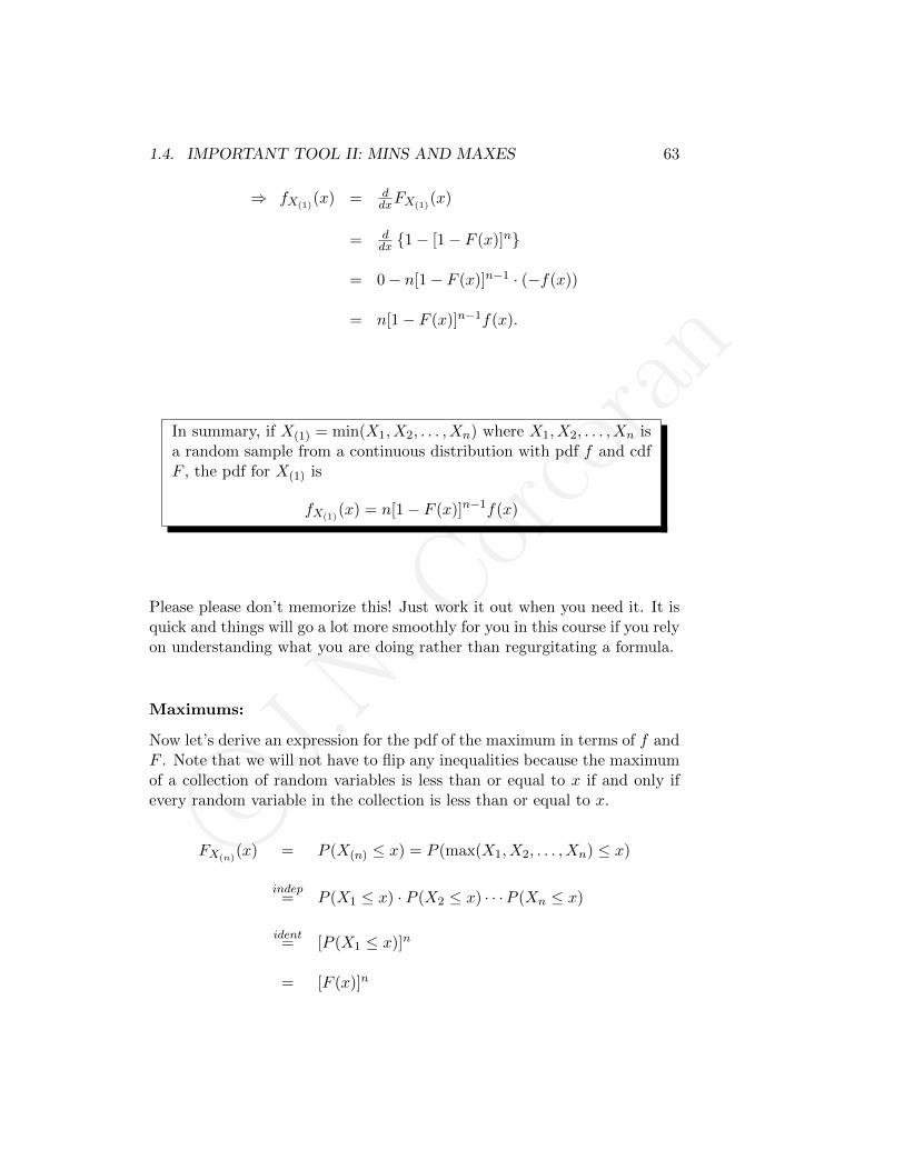
c©J.N.Corcoran
1.4. IMPORTANT TOOL II: MINS AND MAXES 63
⇒ fX(1)(x) = d
dxFX(1)(x)
= ddx 1− [1− F (x)]n
= 0− n[1− F (x)]n−1 · (−f(x))
= n[1− F (x)]n−1f(x).
In summary, if X(1) = min(X1, X2, . . . , Xn) where X1, X2, . . . , Xn isa random sample from a continuous distribution with pdf f and cdfF , the pdf for X(1) is
fX(1)(x) = n[1− F (x)]n−1f(x)
Please please don’t memorize this! Just work it out when you need it. It isquick and things will go a lot more smoothly for you in this course if you relyon understanding what you are doing rather than regurgitating a formula.
Maximums:
Now let’s derive an expression for the pdf of the maximum in terms of f andF . Note that we will not have to flip any inequalities because the maximumof a collection of random variables is less than or equal to x if and only ifevery random variable in the collection is less than or equal to x.
FX(n)(x) = P (X(n) ≤ x) = P (max(X1, X2, . . . , Xn) ≤ x)
indep= P (X1 ≤ x) · P (X2 ≤ x) · · ·P (Xn ≤ x)
ident= [P (X1 ≤ x)]n
= [F (x)]n

c©J.N.Corcoran
64CHAPTER 1. MATHSTAT PRELIMINARIES: FOUR IMPORTANT TOOLS FORMATHEMATICAL STATISTICS
⇒ fX(n)(x) = d
dxFX(n)(x)
= ddx [F (x)]n
= n[F (x)]n−1 · f(x)
In summary, if X(n) = max(X1, X2, . . . , Xn) where X1, X2, . . . , Xn isa random sample from a continuous distribution with pdf f and cdfF , the pdf for X(n) is
fX(n)(x) = n[F (x)]n−1 · f(x)
Again, I’m begging you not to memorize this! It’s easy to derive!
For fun, you might want to work out the pdf of the maximum of exponentialrandom variables. The resulting pdf is not from a nice “named” distributionthat you will find on your table. Similarly, not all transformations of pdfsfor random variables, such as in Section 1.2 will result in recognizable pdfs.
1.5 Important Tool IV: Moment Generating Func-tions (MGFs)
For a random variableX, the moment generating function (mgf),denoted by M(t) or MX(t) if necessary, is defined as
M(t) = E[etX ].
(If it becomes necessary to distinguish between two moment generating func-tions, for random variables X and Y , we will write MX(t) and MY (t).)
Moment generating functions are extremely useful tools for both computing“moments” of distributions which are the expectations E[X], E[X2], E[X3],. . ., and for identifying distributions of some transformed random variables.Most notably, if you are asked to find the distribution of the “big fat sum”
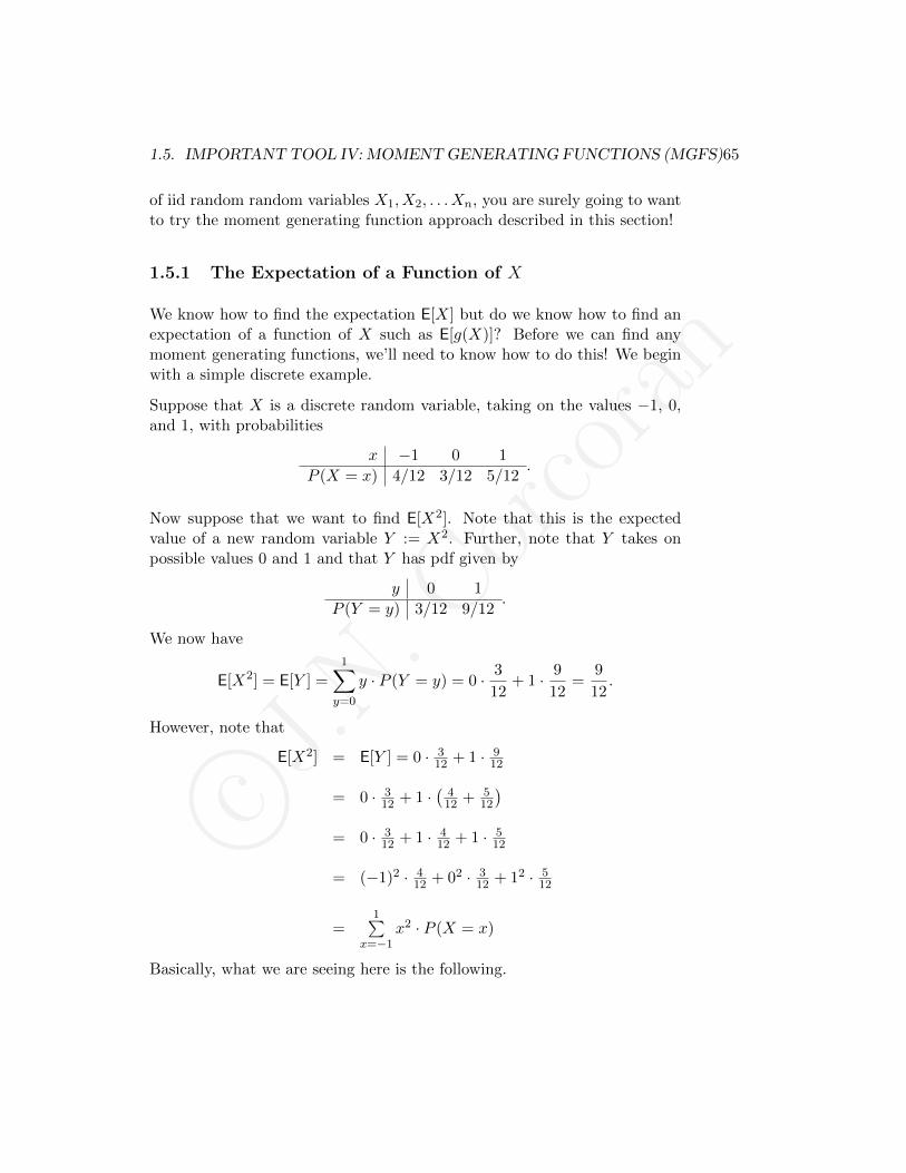
c©J.N.Corcoran
1.5. IMPORTANT TOOL IV: MOMENTGENERATING FUNCTIONS (MGFS)65
of iid random random variables X1, X2, . . . Xn, you are surely going to wantto try the moment generating function approach described in this section!
1.5.1 The Expectation of a Function of X
We know how to find the expectation E[X] but do we know how to find anexpectation of a function of X such as E[g(X)]? Before we can find anymoment generating functions, we’ll need to know how to do this! We beginwith a simple discrete example.
Suppose that X is a discrete random variable, taking on the values −1, 0,and 1, with probabilities
x −1 0 1
P (X = x) 4/12 3/12 5/12.
Now suppose that we want to find E[X2]. Note that this is the expectedvalue of a new random variable Y := X2. Further, note that Y takes onpossible values 0 and 1 and that Y has pdf given by
y 0 1
P (Y = y) 3/12 9/12.
We now have
E[X2] = E[Y ] =1∑y=0
y · P (Y = y) = 0 · 3
12+ 1 · 9
12=
9
12.
However, note that
E[X2] = E[Y ] = 0 · 312 + 1 · 9
12
= 0 · 312 + 1 ·
(412 + 5
12
)= 0 · 3
12 + 1 · 412 + 1 · 5
12
= (−1)2 · 412 + 02 · 3
12 + 12 · 512
=1∑
x=−1x2 · P (X = x)
Basically, what we are seeing here is the following.

c©J.N.Corcoran
66CHAPTER 1. MATHSTAT PRELIMINARIES: FOUR IMPORTANT TOOLS FORMATHEMATICAL STATISTICS
Let X be a random variable with pdf fx(x). Let g(x) be some func-tion.• If X is discrete, we have have
E[g(X)] =∑x
g(x)fX(x).
• If X is continuous, we have have
E[g(X)] =
∫ ∞−∞
g(x)fX(x) dx.
So, even though g(X) is a new random variable, when finding E[g(X)] it isunnecessary to find a new pdf! That’s kind of surprising if you think aboutit... but a lot of people don’t think about it– they just do it sort of naturallywithout realizing how big of a deal this is. This is why this new formula forE[g(X)] (in either the discrete or continuous case) is known as the Law ofthe Unconscious Statistician!
We will now prove the formula for E[g(X)] in the case where X is continuousand g is invertible and differentiable. Proofs of the other cases are omitted.
Suppose that X is continuous and g is a nice invertible and differentiablefunction. Define Y = g(X). Then, since we know from Section 1.2 that
fY (y) = fX(g−1(y))∣∣∣ ddyg−1(y)
∣∣∣, we have that
E[g(X)] = E[Y ] =∫∞−∞ y · fY (y) dy
=∫∞−∞ y · fX(g−1(y))
∣∣∣ ddyg−1(y)∣∣∣ dy
Since g is invertible, we know that it is either strictly increasing or strictlydecreasing. Let’s consider each case separately.
Case One: g is strictly increasing
If g is strictly increasing then g−1 is as well. So, the derivative ddyg−1(y) is
always positive and we can drop the absolute value in the above integral.We now have
E[g(X)] =
∫ ∞−∞
y · fX(g−1(y)) · ddyg−1(y) dy
c©J.N.Corcoran
1.5. IMPORTANT TOOL IV: MOMENTGENERATING FUNCTIONS (MGFS)67
Consider the change of variable x = g−1(y). Note that dx = ddyg−1(y) dy.
Making the substitution, we have
E[g(X)] =
∫ ?′
?g(x) · fX(x)dx
for some limits of integration ? and ?′.
As for the limits, note that, even the original limits of integration went from−∞ to ∞, they might actually have ended up being cut off by the supportset for the pdf fY (y). That is, the pdf fY (y) may only be non-zero on somesmaller interval. Furthermore, even if y = g(x) does go from −∞ to ∞,the inverse might not. For example, if y = g(x) = lnx, then y goes from−∞ to ∞, but x = g−1(y) only takes values from 0 to ∞. However, in thisexample, ∫ ∞
0g−1(x) fX(x) dx =
∫ ∞−∞
g−1(x) fX(x) dx
because the pdf for X will be zero outside of (0,∞).
So, when we make the substitution x = g−1(y), it will be safe to have limitsall the way from −∞ to ∞ since g−1 is increasing and since the pdf will cutoff the limits in the appropriate places. That is, it is safe to use the limits? = −∞ and ?′ =∞ and we have
E[g(X)] =
∫ ∞−∞
g(x)fX(x) dx,
as desired.
Case One: g is strictly decreasing
If g is strictly decreasing then g−1 is as well. So, the derivative ddyg−1(y) is
always negative and we have that | ddyg−1(y)| = − d
dyg−1(y). Thus, we have
thatE[g(X)] =
∫∞−∞ y · fX(g−1(y))
∣∣∣ ddyg−1(y)∣∣∣ dy
= −∫∞−∞ y · fX(g−1(y)) · ddyg
−1(y)
Making the substitution x = g−1(y) and again noting that dx = ddyg−1(y),
we have that
E[g(X)] = −∫ ?′
?g(x) · fX(x)dx
for some limits of integration ? and ?′.
c©J.N.Corcoran
68CHAPTER 1. MATHSTAT PRELIMINARIES: FOUR IMPORTANT TOOLS FORMATHEMATICAL STATISTICS
Since g−1 is a decreasing function, as y increases, x = g−1(y) decreases.As per the discussion in the increasing case, even if the random variable Xtakes on only a limited range of values, we can let x decrease from∞ all theway to −∞ and the pdf will cut us off appropriately. Thus,
E[g(X)] = −∫ −∞∞
g(x) · fX(x)dx =
∫ ∞−∞
g(x) · fX(x),
as desired.
Now that we know how to compute the expectation of a function of a randomvariable, we can get back to moment generating functions!
1.5.2 Finding MGFs and the Poisson Distribution
A Discrete Example:
A discrete random variable X is said to have the Poisson distributionwith parameter λ if X has pdf.
f(x) = P (X = x) =e−λλx
x!I0,1,2,...(x).
We write X ∼ Poisson(λ).
Recall how we motivated the exponential distribution. We imagined events(arrivals at the door of a grocery store) occurring with two assumptions.They were that
1. the arrival/event rate is a constant λ per unit time, and
2. the number of arrivals/events in non-overlapping periods of time areindependent.
Under these assumptions, the exponential distribution describes the amountof time between any two consecutive arrivals/events. One can show (Again,I’d direct you to take APPM 4/5560 where this scenario is a core focus!)
c©J.N.Corcoran
1.5. IMPORTANT TOOL IV: MOMENTGENERATING FUNCTIONS (MGFS)69
that the number of arrivals in one unit of time has the Poisson distributionwith parameter λ.
So, suppose that X ∼ Poisson(λ). Let us find the moment generatingfunction for X. Since this is a discrete random variable, the expectation iscomputed as a sum and not an integral.
MX(t) = E[etX ] =∑
x etx · P (X = x)
=∑∞
x=0 etx e−λλx
x!
=∑∞
x=0e−λ(λet)x
x!
At this point, you could pull out the e−λ and recall the Taylor series expan-sion of ex is
ex =∞∑k=0
xk
k!.
In out moment generating function expression, the k is actually x and thex is λet. So,
MX(t) = e−λ∞∑x=0
(λet)x
x!= e−λ eλe
t= eλ(et−1).
Alternatively, you could do what will become our “standard MathStat trick”that we usually use for integrals. The sum we need to compute looks almostlike the sum over all values of the Poisson pdf except, in place of λ, we haveλet. To make it into the Poisson pdf, we need the “e−λ part” which, in thiscase is e−λe
t. Putting this in (after pulling out the e−λ) and adjusting for
it by putting eλt out front, we have
MX(t) =∑∞
x=0e−λ(λet)x
x!
= eλ(et−1)∞∑x=0
e−λet(λet)x
x!︸ ︷︷ ︸sum of Poisson
pdf is 1
= eλ(et−1).
c©J.N.Corcoran
70CHAPTER 1. MATHSTAT PRELIMINARIES: FOUR IMPORTANT TOOLS FORMATHEMATICAL STATISTICS
(Make sure you can find this in the moment generating column on the tableof distributions!)
A Continuous Example:
Let X ∼ exp(rate = λ). Let us find the mgf of X.
MX(t) = E[etX ] =∫∞−∞ e
tx f(x) dx
=∫∞
0 etx λe−λx dx
=∫∞
0 λe−λx+tx dx
To integrate, it is convenient to factor out the x in that exponent so we areintegrating something like ecx. However, by taking out the negative as well,we can see something that looks like the exponential pdf with λ− t in placeof λ.
MX(t) =
∫ ∞0
λe−(λ−t)x dx
Note that, in order for this integral to converge we must have λ − t > 0,otherwise the integrand is blowing up. (Alternatively, when comparing thisto the exponential pdf, the usual parameter restriction λ > 0 has becomeλ− t > 0.) Either way you look at it, this mgf is only defined for t < λ.
So, for t < λ,
MX(t) =∫∞
0 λe−(λ−t)x dx
= λλ−t
∫∞0 (λ− t)e−(λ−t)x dx
= λλ−t · 1 = λ
λ−t
since that integral is that of a pdf over its entire support.
1.5.3 Finding Moments
For a random variable X, or its associated distribution, “moments” areexpectations of the form E[Xk] for k = 1, 2, 3, . . .. (Sometimes such mo-ments are called “non-central moments” as opposed to the “central mo-ments” E[(X −µ)k] where X is first “centered” around its mean µ = E[X].)
c©J.N.Corcoran
1.5. IMPORTANT TOOL IV: MOMENTGENERATING FUNCTIONS (MGFS)71
Consider taking a derivative with respect to t of the moment generatingfunction MX(t).
MX(t) = E[etX ] ⇒ M ′X(t) =d
dtMX(t) =
d
dtE[etX ]
?= E
[d
dtetX]
= E[XetX ]
At that question mark, we pulled a derivative inside of an expectation. Sincean expectation is a sum or integral, we really just exchanged a derivativeand a sum or integral. In general, this may or may not be a valid thing todo. If the sum/integral converges and the sum/integral of the differentiatedintegrand also converges, they will converge to the same thing. For thiscourse, things are mostly well behaved and you may assume thisexchange is always valid.
Now,
M ′X(0) = E[Xe0] = E[X].
So, we see that by differentiating the moment generating function and plug-ging in a 0 we get the first moment of this distribution!
With a second derivative, we have
M ′′X(t) =d
dtM ′X(t) =
d
dtE[XetX ] = E
[d
dtXetX
]= E[X2etX ].
So, plugging in a 0 now gives us
M ′′X(0) = E[X2e0] = E[X2],
giving us the second moment of the distribution.
In general, for a random variable X with mgf MX(t), the kth momentis obtained by M (k)(0), where M (k)(t) is the kth derivative of MX(t)with respect to t.
Discrete Example:
Let X ∼ Poisson(λ). One can show, using the definition of expectationand variance that E[X] = λ and V ar[X] = λ. While the variance is a bitmessy, you should try to show that E[X] = λ using our “summing without
c©J.N.Corcoran
72CHAPTER 1. MATHSTAT PRELIMINARIES: FOUR IMPORTANT TOOLS FORMATHEMATICAL STATISTICS
summing” trick of rewriting things so that you are ultimately summing apdf over its entire support.
Let us now find the mean and variance for the Poisson distribution usingmoment generating functions. Recall that MX = exp[λ(et − 1)]. (That“exp” notation is another way to write e to a power.)
So,M ′X(t) = exp[λ(et − 1)] · ddt [λ(et − 1)]
= exp[λ(et − 1)] · λet
⇒ E[X] = M ′X(0) = λ.
Furthermore,
M ′′X(t) = exp[λ(et − 1)] · λet + λet · exp[λ(et − 1)] · λet
= λet · exp[λ(et − 1)] · (1 + λet)
⇒ M ′′X(0) = λ(1 + λ) = λ+ λ2.
So, we have that
V ar[X] = E[X2]− (E[X])2 = λ+ λ2 − (λ)2 = λ,
as desired.
1.5.4 The MGF Uniquely Identifies the Distribution
Here is an exciting claim.
A moment generating function for a random variable X uniquelydetermines its distribution!
For example, if you compute the mgf for some random variable X and get,for example, exp[λ(et−1)], you know that X must be a Poisson(λ) randomvariable!

c©J.N.Corcoran
1.5. IMPORTANT TOOL IV: MOMENTGENERATING FUNCTIONS (MGFS)73
This claim is arguably one of the most important reasons for learning aboutmoment generating functions. A full proof is beyond the scope of this course,but I will eventually include a proof in these notes in a simplified setting. Fornow, I need to get more notes out, so let’s assume the claim is true. It is es-pecially useful for finding the distribution of sums of independentrandom variables.
Example:
LetX1, X2, . . . , Xn be independent random variables withXi ∼ Poisson(λi).
Note that these are not “iid” random variables. For this example, the ran-dom variables are not identically distributed. Although they all have aPoisson distribution, the changing λ’s make them different Poisson distribu-tions.
Let us find the distribution of Y =∑n
i=1Xi.
MY (t) = E[etY ] = E[et∑Xi
]= E
[∏ni=1 e
tXi]
indep=
∏ni=1 E[etXi ] =
∏ni=1MXi(t)
=∏ni=1 exp[λi(e
t − 1)]
= exp[(∑λi)(e
t − 1)]
Since this is the mgf of the Poisson distribution with rate∑n
i=1 λi, we canconclude that
Y ∼ Poisson (∑n
i=1 λi) .
That was a lot easier than what would have been a generalized (to n dimen-sions) Jacobian approach to finding the distribution and even easier thanthe only slightly less cumbersome “conditioning approach” that you wouldstudy in a stochastic process course such as APPM 4/5560. (Just take italready so I can stop the advertisements!)
An Important Example:
Let X1, X2, . . . , Xn be iid random variables from any distribution. Let Y =∑ni=1Xi.
c©J.N.Corcoran
74CHAPTER 1. MATHSTAT PRELIMINARIES: FOUR IMPORTANT TOOLS FORMATHEMATICAL STATISTICS
Since all of the Xi share the same pdf, let’s call it f , the expectations E[etXi ]and E[etXj ] are the same. They will both be the sum or integral of etx timesthe pdf f(x). Thus, by going through the same calculations as in the Poissonexample above, it is easy to see that
MY (t) = [MX1(t)]n .
This will be so useful that it deserves a box.
If X1, X2, . . . , Xn be iid random variables from a distribution withmoment generating function MX(t). The sum Y =
∑ni=1Xi has
moment generating function MY (t) = [MX(t)]n. Here, X is used todenote any of the Xi.
So, for example, X1, X2, . . . , Xniid∼ Poisson(λ), Y =
∑ni=1Xi has mgf
MY (t) = [MX(t)]n =[exp[λ(et − 1)]
]n= exp[λn(et − 1)],
which is the mgf for the Poisson distribution with rate λn. So, we knowthat Y ∼ Poisson(λn).
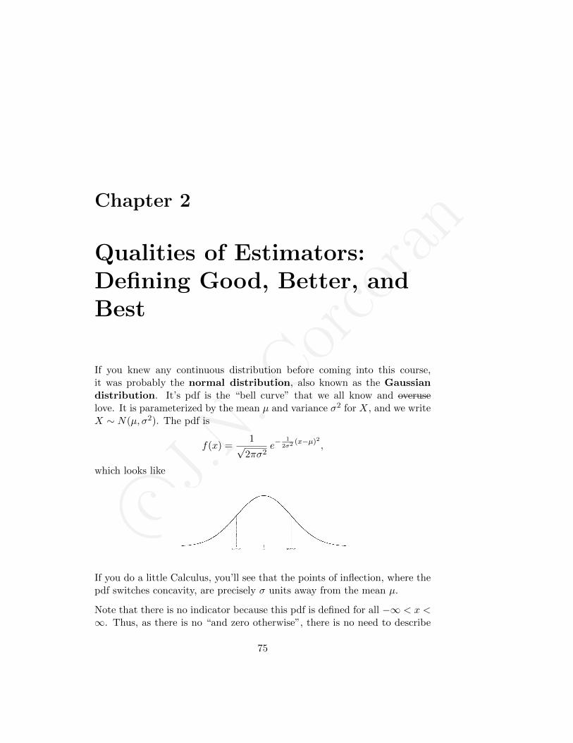
c©J.N.Corcoran
Chapter 2
Qualities of Estimators:Defining Good, Better, andBest
If you knew any continuous distribution before coming into this course,it was probably the normal distribution, also known as the Gaussiandistribution. It’s pdf is the “bell curve” that we all know and overuselove. It is parameterized by the mean µ and variance σ2 for X, and we writeX ∼ N(µ, σ2). The pdf is
f(x) =1√
2πσ2e−
12σ2
(x−µ)2 ,
which looks like
If you do a little Calculus, you’ll see that the points of inflection, where thepdf switches concavity, are precisely σ units away from the mean µ.
Note that there is no indicator because this pdf is defined for all −∞ < x <∞. Thus, as there is no “and zero otherwise”, there is no need to describe
75
c©J.N.Corcoran
76CHAPTER 2. QUALITIES OF ESTIMATORS: DEFININGGOOD, BETTER, AND BEST
the support with an indicator. If we did, it would be I(−∞),∞(x), which isalways 1. For fun, why don’t you multiply every function you write downtoday by 1!
Estimation:
Let X1, X2, . . . , Xn be a random sample from the N(µ, 1) distribution. If nis large and if you make a histogram of your sampled values, you should seethe histogram roughly matching up with the pdf for the N(µ, 1) distribution.In particular, you will see the majority of sampled values towards the center(which is µ) and not so many out “in the tails’.”
Question: How might you estimate the mean µ?
Answer: The most “natural” answer would be to use the sample mean:
X =1
n
n∑i=1
Xi.
The true mean µ for the distribution is a probability weighted average. Thesample mean is the average of the sampled values and it already has the“probability weighted” part “built in” since the values are falling mostly inthe high probability regions and not so much in the low probability regions.
We will use the notation µ to denote an estimator for µ. So, we write
µ = X.
Note that the X in “X bar” is capitalized. At this point we are consideringit as a random variable. We are going, in the future, to sample valuesX1, X2, . . . , Xn from this normal distribution and then we are going to av-erage them. Once we do, we will have observations x1, x2, . . . , xn which havesample mean x. The word “estimator” is used to refer to the random vari-able X while the word “estimate” is used to refer to the actual observationx.
Estimating the mean µ with the sample mean X seems like the “obvious”thing to do. However, the following questions arise.
1. How “good” is this estimator? What does “good” even mean?
c©J.N.Corcoran
2.1. NOTATION, STATISTICS, AND UNBIASEDNESS 77
2. Can we do better?
3. How would you go about estimating parameters with a less obviousinterpretation, such as the α from the Γ(α, β) distribution?
Before we can propose good estimators for parameters of various distribu-tions, we need to be able to talk about several measures of the quality of anestimator so that we know where to aim.
2.1 Notation, Statistics, and Unbiasedness
We will use θ to denote a general parameter. It might represent µ in a normaldistribution, λ in the exponential distribution, β in a gamma distribution,or a number of other things. It might even represent a vector of parameterssuch as θ = (µ, σ2) or θ = (α, β).
From now on, we really want to emphasize that our pdfs have parameters.So, instead of writing f(x), we will write f(x; θ). The semicolon will beused to separate variables and parameters. For example, when referring toa joint pdf for X1, X2, . . . , Xn with parameters α and β, we might writef(x1, x2, . . . , xn;α, β).
Let X1, X2, . . . , X2 be a random sample from the distribution with pdff(x; θ).
The Goal:
The goal is to estimate the parameter θ or some function of the parameterτ(θ) based on what we see in the random sample X1, X2, . . . , Xn.
Our estimator will be a statistic which is defined as some function of thedata. A statistic is a random variable that we will denote
T = t(X1, X2, . . . , Xn) = t( ~X).
When estimating τ(θ) using the statistic T = t( ~X), one thing we might wantis for the estimator to be “on average” correct.

c©J.N.Corcoran
78CHAPTER 2. QUALITIES OF ESTIMATORS: DEFININGGOOD, BETTER, AND BEST
We say that T is an unbiased estimator for τ(θ) if
E[T ] = τ(θ).
It seems that it is a good time to review some properties of expectation.
2.2 Expectation, Variance, and Covariance Review

c©J.N.Corcoran
Appendix A
Tables of Distributions
79
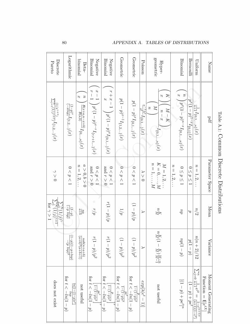
c©J.N.Corcoran
80 APPENDIX A. TABLES OF DISTRIBUTIONS
Tab
leA
.1:Com
mon
Discrete
Distrib
ution
s
Nam
ep
df
Param
eterS
pace
Mean
Varian
ceM
omen
tG
eneratin
gF
un
ction=
E[etX
]
Un
iform1
n+
1 I0,1,...,n (x
)n
=1,2,...
n/2
n(n
+2)/
12∑
nj=0
1n
+1 ejt
=1−e(n
+1)t
(n+
1)(1−
et)
Bern
oulli
px(1−p)1−xI
0,1 (x
)0≤p≤
1p
p(1−p)
(1−p)
+pet
Bin
omial
(nx )
px(1−p)n−
xI0,1,...,n (x
)0≤p≤
1np
np(1−p)
[(1−p)
+pet] n
n=
1,2,...
Hyp
er-geo
metric
Kx
M−K
n−x
Mn
I0,1,...,n (x
)M
=1,2
,...K
=0,...,M
n=
1,...,MnKM
nKM
(1−
KM)M−n
M−
1n
otu
seful
Poisso
ne −λλx
x!I
0,1,... (x
)λ>
0λ
λexp[λ
(et−
1)]
Geom
etricp(1−p)xI
0,1,... (x
)0<p<
1(1−p)/p
(1−p)/p
2p
1−(1−
p)et
fort<−ln
(1−p)
Geom
etricp(1−p)x−
1I1,2,... (x
)0<p<
11/p
(1−p)/p
2pet
1−(1−
p)et
fort<−ln
(1−p)
Neg
ative
Bin
omial
(r
+x−
1x
)pr(1−p)xI
0,1,... (x
)0<p<
1an
dr>
0r(1−p)/p
r(1−p)/p
2
[p
1−(1−
p)et ]r
fort<−ln
(1−p)
Neg
ative
Bin
omial
(x−
1r−
1 )pr(1−p)x−
rIr,r
+1,... (x
)0<p<
1an
dr>
0r/p
r(1−p)/p
2
[pet
1−(1−
p)et ]r
fort<−ln
(1−p)
Beta
-b
inom
ial
(nx )
B(x
+a,n−
x+b)
B(a,b)
I0,...,n (x
)a>
0,b>
0n
=1,2,...
na
a+b
nab(n
+a+b)
(a+b)
2(a
+b+
1)
not
usefu
l
Logarith
mic
(1−p)x
(−xlnp) I
1,2,... (x
)0<p<
1(1−
p)
(−plnp)
(1−p)(1−
p+lnp)
−(p
lnp)2
ln[1−
(1−p)et]
lnp
fort<−ln
(1−p)
Discrete
Pareto
(1/xγ+1)
∑∞j=1(1/jγ+1) I
1,2,... (x
)γ>
0
∑∞1
(1/j)γ
∑∞1
(1/j)γ
+1
forγ>
1
does
not
exist
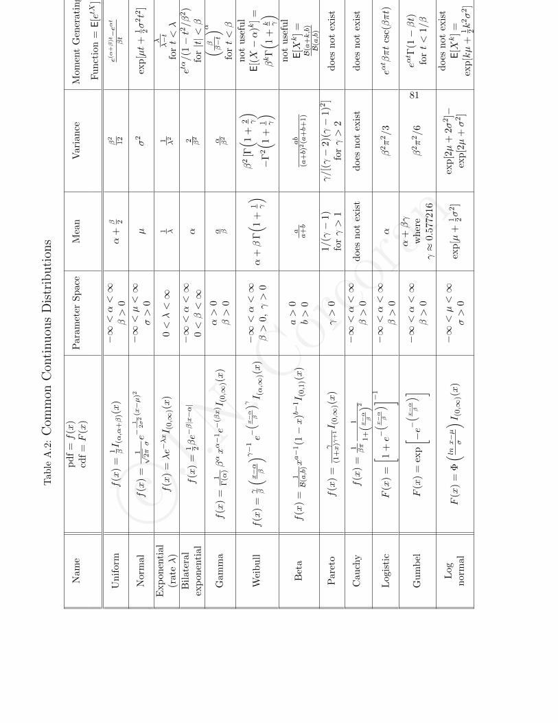
c©J.N.Corcoran
81
Tab
leA
.2:Com
mon
Con
tinuou
sDistribution
s
Nam
ep
df
=f
(x)
cdf
=F
(x)
Par
amet
erS
pac
eM
ean
Vari
ance
Mom
ent
Gen
erat
ing
Fu
nct
ion
=E
[etX
]
Un
ifor
mf
(x)
=1 βI (α,α
+β
)(x
)−∞<α<∞
β>
0α
+β 2
β2
12
e(α+β)t−eαt
βt
Norm
al
f(x
)=
1√
2πσe−
12σ2
(x−µ
)2−∞<µ<∞
σ>
0µ
σ2
exp
[µt
+1 2σ
2t2
]
Exp
onen
tial
(rateλ
)f
(x)
=λe−
λxI (
0,∞
)(x
)0<λ<∞
1 λ1 λ2
λλ−t
fort<λ
Bil
ate
ral
exp
on
enti
alf
(x)
=1 2βe−
β|x−α|
−∞<α<∞
0<β<∞
α2 β2
etα/(
1−t2/β
2)
for|t|<β
Gam
ma
f(x
)=
1Γ
(α)βαxα−
1e−
(βx
) I(0,∞
)(x
)α>
0β>
0α β
α β2
( β β−t
) αfo
rt<β
Wei
bu
llf
(x)
=γ β
( x−α β) γ−1
e−( x−
αβ
) γ I (α,∞
)(x
)−∞<α<∞
β>
0,γ>
0α
+β
Γ( 1
+1 γ
)β
2[Γ( 1
+2 γ
)−
Γ2( 1
+1 γ
)n
ot
use
ful
E[(X−α
)k]
=
βkΓ( 1
+k γ
)B
eta
f(x
)=
1B
(a,b
)xa−
1(1−x
)b−
1I (
0,1
)(x
)a>
0b>
0aa+b
ab
(a+b)
2(a
+b+
1)
not
use
ful
E[X
k]
=B
(a+k,b
)B
(a,b
)
Par
eto
f(x
)=
γ(1
+x
)γ+1I (
0,∞
)(x
)γ>
01/
(γ−
1)fo
rγ>
1γ/[
(γ−
2)(γ−
1)2
]fo
rγ>
2d
oes
not
exis
t
Cau
chy
f(x
)=
1 βπ
1
1+( x−
αβ
) 2−∞<α<∞
β>
0d
oes
not
exis
td
oes
not
exis
td
oes
not
exis
t
Logis
tic
F(x
)=
[ 1+e−( x−
αβ
)] −1−∞<α<∞
β>
0α
β2π
2/3
eαt βπt
csc(βπt)
Gu
mb
elF
(x)
=ex
p
[ −e−( x−
αβ
)]−∞<α<∞
β>
0
α+βγ
wh
ere
γ≈
0.5
772
16β
2π
2/6
eαt Γ
(1−βt)
fort<
1/β
Log
norm
alF
(x)
=Φ( lnx
−µ
σ
) I (0,∞
)(x
)−∞<µ<∞
σ>
0ex
p[µ
+1 2σ
2]
exp
[2µ
+2σ
2]−
exp
[2µ
+σ
2]
does
not
exis
tE
[Xk]
=ex
p[kµ
+1 2k
2σ
2]

c©J.N.Corcoran
82 APPENDIX A. TABLES OF DISTRIBUTIONS

c©J.N.Corcoran
Appendix B
The Jacobian and a Changeof Variables
B.1 The Jacobian
For a single integral, the substitution x = x(u) gives us∫ x2
x1
f(x) dx =
∫ u2
u1
f(x(u))dx
dudu
For double integrals, we consider a change of variables from the x1x2-planeto the y1y2-plane, where
y1 = g1(x1, x2) and y2 = g2(x1, x2).
We asume we can solve these equations for x1 and x2:
x1 = g−11 (y1, y2) and x2 = g−1
2 (y1, y2).
Now, consider with a small rectangle R in the x1x2-plane whose lower left
corner is the point (x(0)1 , x
(0)2 ) and whose dimensions are ∆x1 and ∆x2.
The image of R in the y1y2-plane is a region S, one of whose boundary
points is (y(0)1 , y
(0)2 ) = (g1(x
(0)1 , x
(0)2 ), g2(x
(0)1 , x
(0)2 )).
The vector~v(x1, x2) = g1(x1, x2)~i+ g2(x1, x2)~j
83
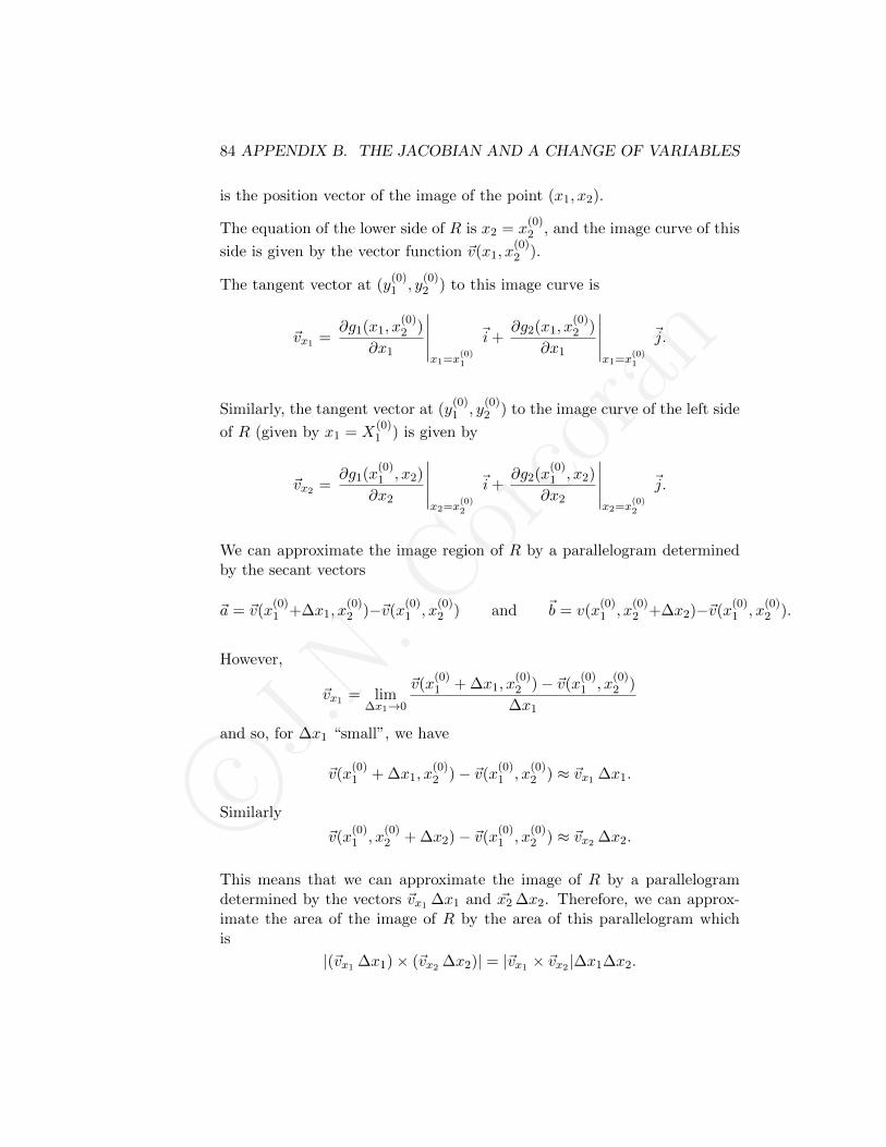
c©J.N.Corcoran
84 APPENDIX B. THE JACOBIAN AND A CHANGE OF VARIABLES
is the position vector of the image of the point (x1, x2).
The equation of the lower side of R is x2 = x(0)2 , and the image curve of this
side is given by the vector function ~v(x1, x(0)2 ).
The tangent vector at (y(0)1 , y
(0)2 ) to this image curve is
~vx1 =∂g1(x1, x
(0)2 )
∂x1
∣∣∣∣∣x1=x
(0)1
~i+∂g2(x1, x
(0)2 )
∂x1
∣∣∣∣∣x1=x
(0)1
~j.
Similarly, the tangent vector at (y(0)1 , y
(0)2 ) to the image curve of the left side
of R (given by x1 = X(0)1 ) is given by
~vx2 =∂g1(x
(0)1 , x2)
∂x2
∣∣∣∣∣x2=x
(0)2
~i+∂g2(x
(0)1 , x2)
∂x2
∣∣∣∣∣x2=x
(0)2
~j.
We can approximate the image region of R by a parallelogram determinedby the secant vectors
~a = ~v(x(0)1 +∆x1, x
(0)2 )−~v(x
(0)1 , x
(0)2 ) and ~b = v(x
(0)1 , x
(0)2 +∆x2)−~v(x
(0)1 , x
(0)2 ).
However,
~vx1 = lim∆x1→0
~v(x(0)1 + ∆x1, x
(0)2 )− ~v(x
(0)1 , x
(0)2 )
∆x1
and so, for ∆x1 “small”, we have
~v(x(0)1 + ∆x1, x
(0)2 )− ~v(x
(0)1 , x
(0)2 ) ≈ ~vx1 ∆x1.
Similarly
~v(x(0)1 , x
(0)2 + ∆x2)− ~v(x
(0)1 , x
(0)2 ) ≈ ~vx2 ∆x2.
This means that we can approximate the image of R by a parallelogramdetermined by the vectors ~vx1 ∆x1 and ~x2 ∆x2. Therefore, we can approx-imate the area of the image of R by the area of this parallelogram whichis
|(~vx1 ∆x1)× (~vx2 ∆x2)| = |~vx1 × ~vx2 |∆x1∆x2.
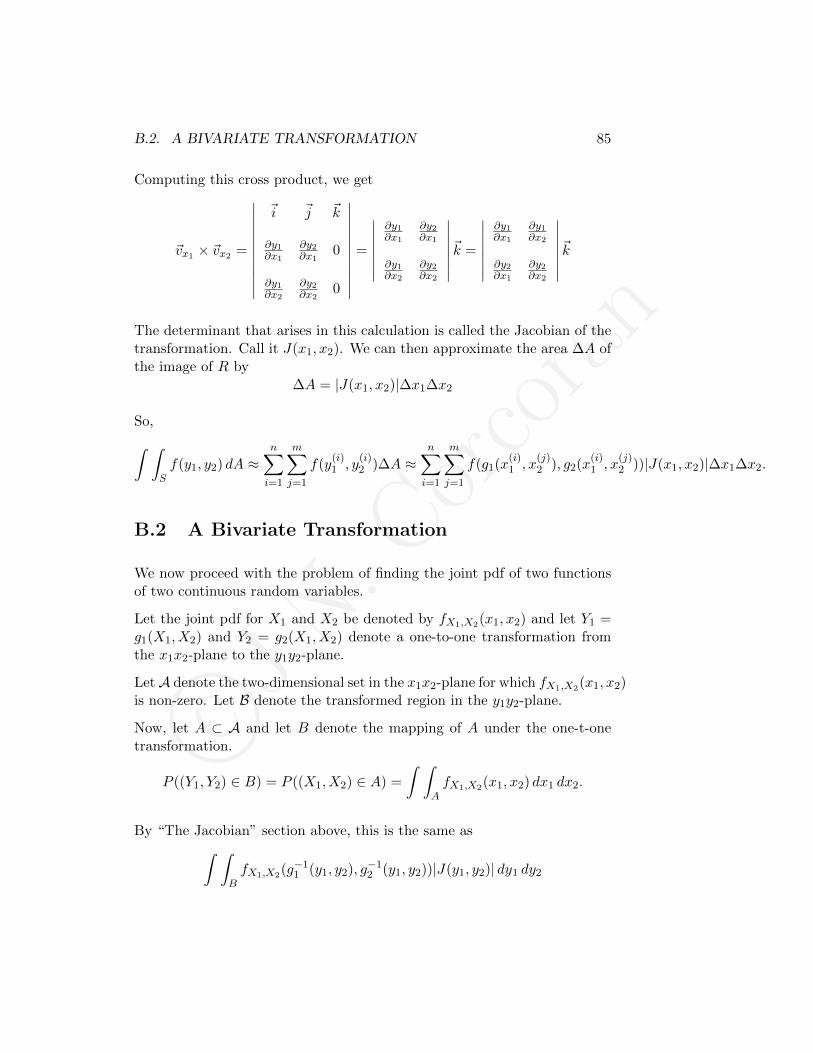
c©J.N.Corcoran
B.2. A BIVARIATE TRANSFORMATION 85
Computing this cross product, we get
~vx1 × ~vx2 =
∣∣∣∣∣∣∣∣∣∣∣
~i ~j ~k
∂y1∂x1
∂y2∂x1
0
∂y1∂x2
∂y2∂x2
0
∣∣∣∣∣∣∣∣∣∣∣=
∣∣∣∣∣∣∣∂y1∂x1
∂y2∂x1
∂y1∂x2
∂y2∂x2
∣∣∣∣∣∣∣~k =
∣∣∣∣∣∣∣∂y1∂x1
∂y1∂x2
∂y2∂x1
∂y2∂x2
∣∣∣∣∣∣∣~k
The determinant that arises in this calculation is called the Jacobian of thetransformation. Call it J(x1, x2). We can then approximate the area ∆A ofthe image of R by
∆A = |J(x1, x2)|∆x1∆x2
So,∫ ∫Sf(y1, y2) dA ≈
n∑i=1
m∑j=1
f(y(i)1 , y
(i)2 )∆A ≈
n∑i=1
m∑j=1
f(g1(x(i)1 , x
(j)2 ), g2(x
(i)1 , x
(j)2 ))|J(x1, x2)|∆x1∆x2.
B.2 A Bivariate Transformation
We now proceed with the problem of finding the joint pdf of two functionsof two continuous random variables.
Let the joint pdf for X1 and X2 be denoted by fX1,X2(x1, x2) and let Y1 =g1(X1, X2) and Y2 = g2(X1, X2) denote a one-to-one transformation fromthe x1x2-plane to the y1y2-plane.
LetA denote the two-dimensional set in the x1x2-plane for which fX1,X2(x1, x2)is non-zero. Let B denote the transformed region in the y1y2-plane.
Now, let A ⊂ A and let B denote the mapping of A under the one-t-onetransformation.
P ((Y1, Y2) ∈ B) = P ((X1, X2) ∈ A) =
∫ ∫AfX1,X2(x1, x2) dx1 dx2.
By “The Jacobian” section above, this is the same as∫ ∫BfX1,X2(g−1
1 (y1, y2), g−12 (y1, y2))|J(y1, y2)| dy1 dy2

c©J.N.Corcoran
86 APPENDIX B. THE JACOBIAN AND A CHANGE OF VARIABLES
B.3 More Variables
All of the above can be extended to the case of many variables. That is,if X1, X2, . . . , Xn has joint pdf fX1,X2,...,Xn(x1, x2, . . . , xn) and we considerthe transformations
y1 = g1(x1, x2, . . . , xn)y2 = g2(x1, x2, . . . , xn)...
......
yn = gn(x1, x2, . . . , xn),
then the joint pdf of Y1, Y2, . . . , Yn is given by
fY1,Y2,...,Yn(y1, y2, . . . , yn) = fX1,X2,...,Xn(g−11 (y1, y2, . . . , yn), . . . , g−1
n (y1, y2, . . . , yn))·|J(y1, y2, . . . , yn)|
where
J =
∣∣∣∣∣∣∣∣∣∣
∂x1∂y1
∂x1∂y2
· · · ∂x1∂yn
∂x2∂y1
∂x2∂y2
· · · ∂x2∂yn
......
......
∂xn∂y1
∂xn∂y2
· · · ∂xn∂yn
∣∣∣∣∣∣∣∣∣∣.