an hmm based comparative genomic framework for …
TRANSCRIPT

An HMM-based "Comparative Genomic Framework for
Analyzing Complex Evolutionary Scenarios
Kevin J. Liu!Department of Computer Science!
Rice University

Comparative Genomics: Background

An Example Comparative Genomic Analysis (Nature 423 2003)
55
to detect the genome-wide signature of motif-like conservation. We use these tests to
detect all significant patterns with strong genome-wide conservation, constructing a list
of 72 genome-wide motifs. We compare this list against previously identified regulatory
motifs and show that our method has high sensitivity and specificity, detecting most
previously known regulatory motifs, but also a similar number of novel motifs. In
chapter 4, we assign candidate functions to these novel motifs, and in chapter 5, we study
their combinatorial interactions.
3.4. Conservation properties of known regulatory motifs
We first studied the binding site for one of the best studied transcription factors,
Gal4, whose sequence motif is CGG(N)11CCG (which contains 11 unspecified bases). Gal4
regulates genes involved in galactose utilization, including the GAL1 and GAL10 genes
that are divergently transcribed from a common intergenic region (Figure 3.2). The Gal4
Figure 3.2. Phylogenetic footprinting of the Gal1-Gal10 intergenic region reveals functional nucleotides.
3

Applications of Comparative Genomics
4
(Nature Reviews Genetics 5, 2004)
Detecting regulatory elements
Detecting cancer mutations
(Nature 465, 2010)
Gene finding
And many, many more …©
2007
Nat
ure
Publ
ishi
ng G
roup
http
://w
ww
.nat
ure.
com
/nat
ureb
iote
chno
logy
(Nature Biotechnology 25, 2007)

Almost all comparative genomic approaches assume that genomes have evolved down a tree.
5 (Nature 431, 2004)

• However, it has been shown that: - different genomic regions might evolve down
different trees, and - the set of species might not have evolved in a
strictly diverging manner.
A
0.005 0.005 0.005 0.005 0.002 0.002 0.002 0.005 0.005 0.005 0.005 0.005 0.005 0.005 0.02
Recombination breakpointMutation specific to A-CMutation specific to D-E
Coding region
Gene tree
0
S
0.1
0.05
B
adenylate cyclase
relA1 ppnK mgtE fabI
RNA pseudouridylate synthaseprotozoan/cyanobacterial globin family protein
(MBE 29, 2013)
different gene trees for different regions in the Staph aureus !genomes, due to horizontal gene transfer!

Comparative Genomics: Going Beyond Trees

8
A Machine Learning View of Comparative Genomics
Genomes
Species network!(DAG)!
+!gene trees
A
B
C
A
B
C
Stochastic !Generative !
Model
Observed Data!(Genomic sequences)

Overarching Goal
• For every site in the genome, learn: - the local gene tree along which the site evolved,
and - the evolutionary trajectory that the local gene tree
took within the species network. • We also want a confidence measure for the
inference.
9

My Approach
• Modeling: Combine species networks and hidden Markov models into one unified framework, PhyloNet-HMM.
• Inference: Using genomic sequence data, the task is to learn the model.
10
11
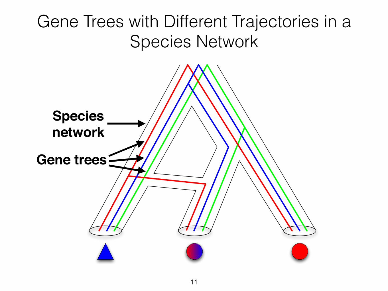
Gene Trees with Different Trajectories in a Species Network
Gene trees
Species !network

Disentangling Gene Tree Trajectories
12

“Pull apart” species network into two “parental trees”
13
Disentangling Gene Tree Trajectories

“Horizontal” and “Vertical” Incongruence
Horizontal!incongruence
14

Horizontal!incongruence
Vertical!incongruence
Vertical!incongruence
“Horizontal” and “Vertical” Incongruence
15

A
B
C
Gene-tree-switching breakpoint
IVI II III V
ψ2 regionψ1 region
A Sequence-Level View of Local Incongruence
g1 g2 g3
ψ1 ψ2
16

Insight #1
• “Horizontal” and “vertical” incongruence between neighboring gene trees represent two different types of dependence.
• Model the two dependence types using two classes of transitions in a graphical model.
17

Insight #2
• DNA sequences are observed, not gene trees. • Under traditional models of DNA sequence
evolution, the probability P(s|g) of observing DNA sequences s given a gene tree g can be efficiently calculated using dynamic programming.
18
Insight #1 + Insight #2 = Use a Hidden Markov
Model (HMM)
19

PhyloNet-HMM: Problem Definition
g1 g2 g3
ψ1 ψ2
20

PhyloNet-HMM: Hidden States
q1 q2 q3
r1 r2 r3
s0
Introgressed
Non-introgressed
21

q1 q2 q3
r1 r2 r3
s0
Introgressed
Non-introgressed
PhyloNet-HMM: Hidden States and Transitions Involving q1
22

PhyloNet-HMM• Each hidden state si is associated with a gene tree g(si)
contained within a “parental” tree f(si)
• The set of HMM parameters λ consists of
- The initial state distribution π
- Transition probabilities
where γ is the “horizontal” parental tree switching frequency.
- The emission probabilities bi = P(Ot|g(si))
23

1. What is the likelihood of the model given the observed DNA sequences?
- Forward algorithm calculates prefix probability
- Backward algorithm calculates suffix probability
- Model likelihood is
2. Which sequence of hidden states best explains the observed DNA sequences? - Posterior decoding probability γt(i) is the probability that HMM is in state si at time t,
calculated as:
3. How do we choose parameter values that maximize the model likelihood?
- Apply hill-climbing to optimize
24
Three Problems Addressed Using PhyloNet-HMM

Related Methods1. Methods that work for at most three genomes, including:
• D-statistic (Durand et al. 2012)
• CoalHMM (Mailund et al. 2012)
2. Methods that consider vertical incongruence or horizontal incongruence but not both, including:
• CoalHMM (Hobolth et al. 2007, Schierup et al. 2009)
• RecHMM (Westesson and Holmes 2009)
25
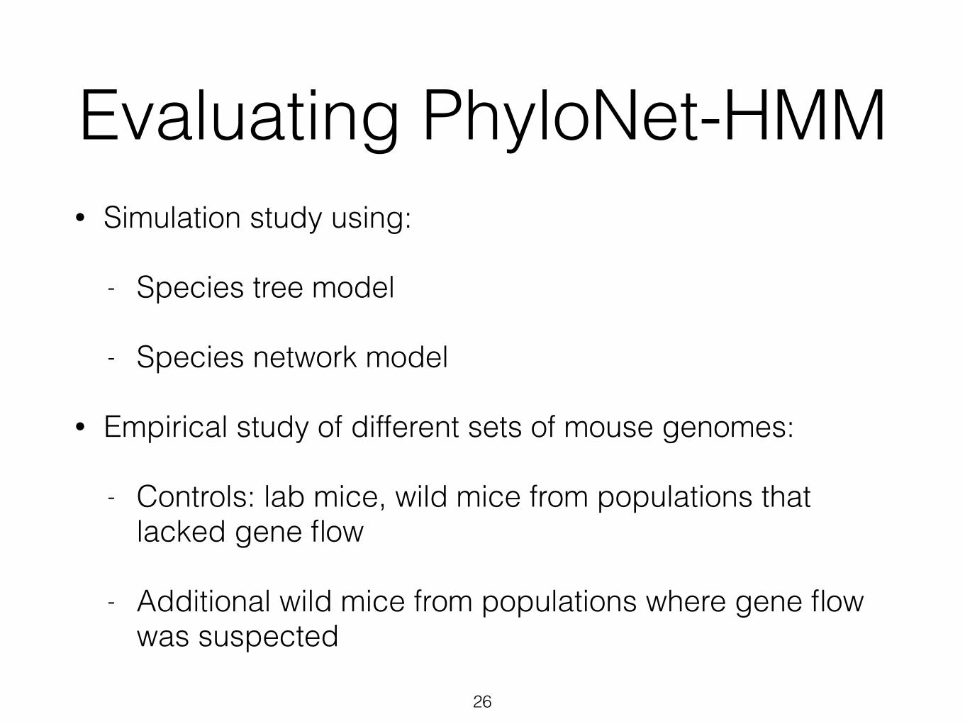
Evaluating PhyloNet-HMM• Simulation study using:
- Species tree model
- Species network model
• Empirical study of different sets of mouse genomes:
- Controls: lab mice, wild mice from populations that lacked gene flow
- Additional wild mice from populations where gene flow was suspected
26

Simulation Model
27
A2 OutgroupB
t0
t1
Mt2
A1

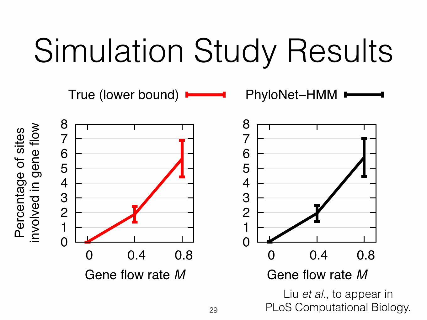
Simulation Study Results
28
0 1 2 3 4 5 6 7 8
0 0.4 0.8Gene flow rate M
True (lower bound)
Per
cent
age
of s
ites
invo
lved
in g
ene
flow
Liu et al., to appear in PLoS Computational Biology.
0 1 2 3 4 5 6 7 8
0 0.4 0.8Gene flow rate M
PhyloNet−HMM
Simulation Study Results
29
0 1 2 3 4 5 6 7 8
0 0.4 0.8Gene flow rate M
True (lower bound)
Per
cent
age
of s
ites
invo
lved
in g
ene
flow
Liu et al., to appear in PLoS Computational Biology.

30
Empirical Study: Non-control Mice (Chromosome 7)
0
0.25
0.5
0.75
1
0 20 40 60 80 100 120 140 160
Prob
abilit
y of
intro
gres
sed
orig
in
Position along chromosome (Mb)
Vkorc1
Liu et al., under review by PNAS.
Pos
terio
r dec
odin
g pr
obab
ility
of ψ
2 sta
te
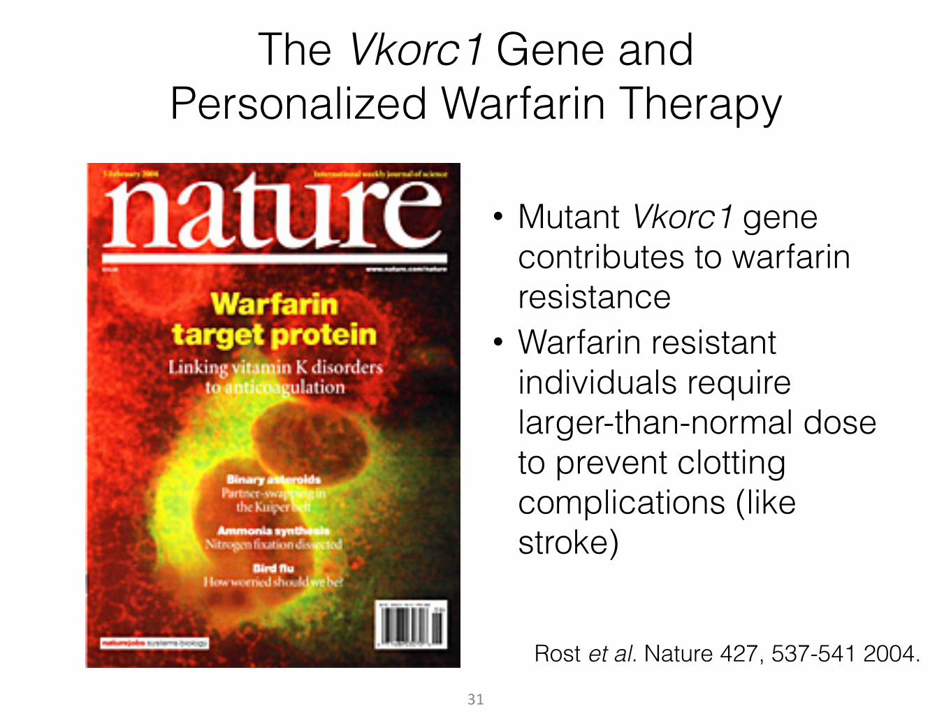
The Vkorc1 Gene and Personalized Warfarin Therapy
Rost et al. Nature 427, 537-541 2004.
• Mutant Vkorc1 gene contributes to warfarin resistance
• Warfarin resistant individuals require larger-than-normal dose to prevent clotting complications (like stroke)
31

Warfarin is ReallyGlorified Rodent
Poison
Reproduced from UTMB. 32
The Spread of Warfarin Resistance in Wild Mice
• Humans inadvertently started a gigantic drug trial by giving warfarin to mice in the wild
• Mice shared genes (including one that confers warfarin resistance) to survive (Song et al. 2011)
- Gene sharing occurred between two different species (introgression)
• To find out results from the drug trial, we just need to analyze the genomes of introgressed mice and locate the introgressed genes
33

Summary and "Future Directions

Summary• PhyloNet-HMM generalizes the basic coalescent model,
one of the most widely used models in population genetics, by using a DAG in place of a tree
• Simulated and empirical data sets with tree-like and non-tree-like evolution were used to validate PhyloNet-HMM
• PhyloNet-HMM found non-tree-like evolution in multiple mouse chromosomes - Introgressed mouse genes confer warfarin resistance,
many with related human genes - New candidate genes to target for improved
personalization of warfarin therapy • Study of non-tree-like evolution is a fundamentally
important research topic in biology35
Future Directions• Future directions include:
- Incorporating network search,
- Detecting adaptive gene flow, and
- Expanding the model and method to account for other evolutionary events (e.g., sequence insertion/deletion).
• Additional biological systems of interest include:
- Bacterial species, where horizontal gene transfer plays an important role in the spread of antibiotic resistance,
- Hybrid plant species, and
- Other introgressed animal species.
36

Acknowledgments
• Supported in part by: –A training fellowship from the Keck Center of the Gulf Coast Consortia, on Rice University’s NLM Training Program in Biomedical Informatics (Grant No. T15LM007093).
–NLM (Grant No. R01LM00949405 to Luay Nakhleh) –NHLBI (Grant No. R01HL09100704 to Michael Kohn)
Luay Nakhleh CS
Michael Kohn Biology
Tandy Warnow CS (UIUC)

Questions?• My website:
http://www.cs.rice.edu/~kl23
• Nakhleh lab website: http://bioinfo.cs.rice.edu
• Warnow lab website: http://www.cs.utexas.edu/~phylo
38

39

40

41

Evolution: Unifying Theme #1
• “Nothing In Biology Makes Sense Except in the Light of Evolution” – 1973 essay by T. Dobzhansky, a famous biologist
• My primary goal: use evolutionary principles to - Create computational methods to analyze
heterogeneous large-scale biological data, - Then apply them to obtain new biological and
biomedical discoveries
42

Num
ber o
f seq
uenc
es
Single gene Entire genome or a few genes
`
Less than1000
1000+
Sequence length
The Pre-genomic Era

My ContributionsN
umbe
r of s
eque
nces
Single gene Entire genome or a few genes
Less than1000
1000+
Graduate work:SATé,
SATé-II,DACTAL,
etc.
Sequence length
Highlight: Liu et al. !“Rapid and Accurate!Large-Scale Co-estimation of !Sequence Alignments and !Phylogenetic Trees,”!Science 2009.

My ContributionsN
umbe
r of s
eque
nces
Single gene Entire genome or a few genes
Less than1000
1000+
Graduate work:SATé,
SATé-II,DACTAL,
etc.
Postgraduate work:PhyloNet-HMM,
etc.
Sequence length

Outline for Today’s TalkN
umbe
r of s
eque
nces
Single gene Entire genome or a few genes
Less than1000
1000+
Graduate work:SATé,
SATé-II,DACTAL,
etc.
Postgraduate work:PhyloNet-HMM,
etc.
Sequence length
Part I: Fast and Accurate Alignment and Tree Estimation
on Large-Scale Datasets

SATé: Simultaneous Alignment and Tree estimation (Liu et al. Science 2009)
• Standard methods for alignment and tree estimation have unacceptably high error and/or cannot analyze large datasets
• SATé has equal or typically better accuracy than all existing methods on datasets with up to thousands of sequences
• 24 hour analyses using standard desktop computer
• SATé-II (Liu et al. Systematic Biology 2012) is more accurate and faster than SATé on datasets with up to tens of thousands of taxa
48
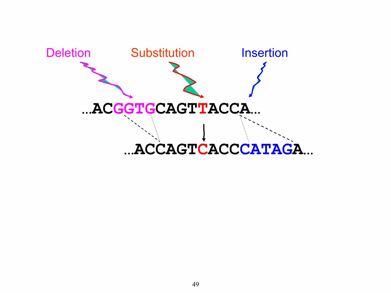
…ACGGTGCAGTTACCA…
Substitution
…ACCAGTCACCCATAGA…
Deletion Insertion
49

…ACGGTGCAGTTACCA…
Substitution
…ACCAGTCACCCATAGA…
Deletion Insertion
The true alignment is:
…ACGGTGCAGTTACC-----A…
…AC----CAGTCACCCATAGA…
50

DNA Sequence Evolution (Example)
AAGACTT -3 mil yrs
-2 mil yrs
-1 mil yrs
today
AAGGCTT AAGACTT
TAGCCCA TAGACTT AGCGAGCAATCGGGCAT
ATCGGGCAT TAGCCCT AGCA
Substitutions Insertions Deletions
51

DNA Sequence Evolution (Example)
-3 mil yrs
-2 mil yrs
-1 mil yrs
today
AAGACTT
TGGACTTAAGGCCT
ATCGGGCAT TAGCCCT AGCA
AAGGCTT TGGACTT
AGCGAGCATAGACTTTAGCCCAATCGGGCAT
52
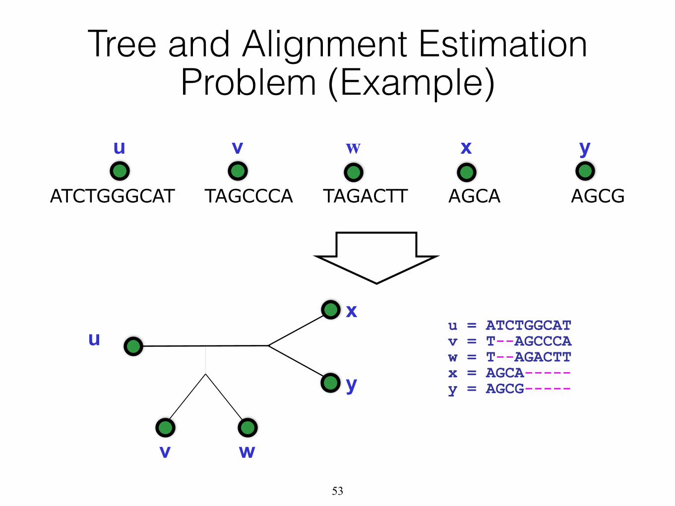
Tree and Alignment Estimation Problem (Example)
TAGCCCA TAGACTT AGCA AGCGATCTGGGCAT
u v w x y
u
v w
x
y
u = ATCTGGCAT v = T--AGCCCA w = T--AGACTT x = AGCA----- y = AGCG-----
53

● Number of trees |T| grows exponentially in n, the number of leaves:
!
● The number of alignments |A| also grows exponentially in n and the length of the longest unaligned sequence.
● All of the common and useful optimization problems are NP-hard.
Many Trees and Many Alignments
54

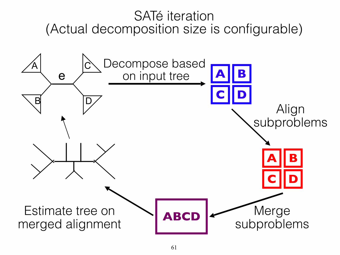
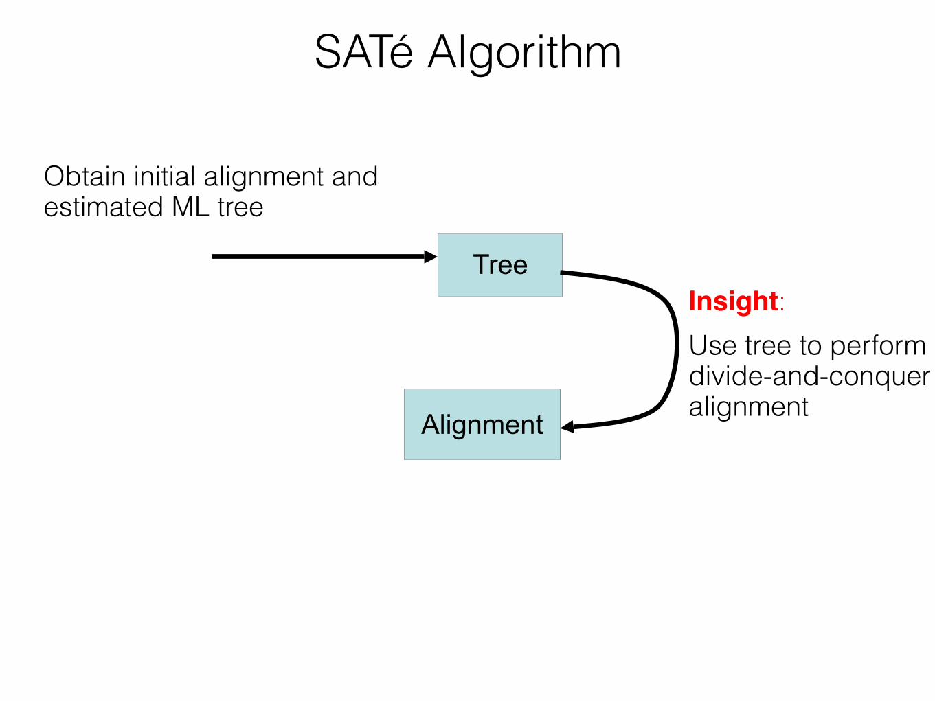
Insight: iterate - use a moderately accurate tree to obtain a more accurate tree If new alignment/tree pair has worse likelihood, realign using a different decomposition Repeat until convergence under the maximum likelihood optimization criterion
SATé Algorithm
Estimate tree on new alignment
TreeObtain initial alignment and tree
Insight:!Use tree to perform divide-and-conquer alignment
Alignment
55

A
B D
Ce
SATé iteration (Actual decomposition size is configurable)
56

A
B D
C Decompose based on input tree A B
C De
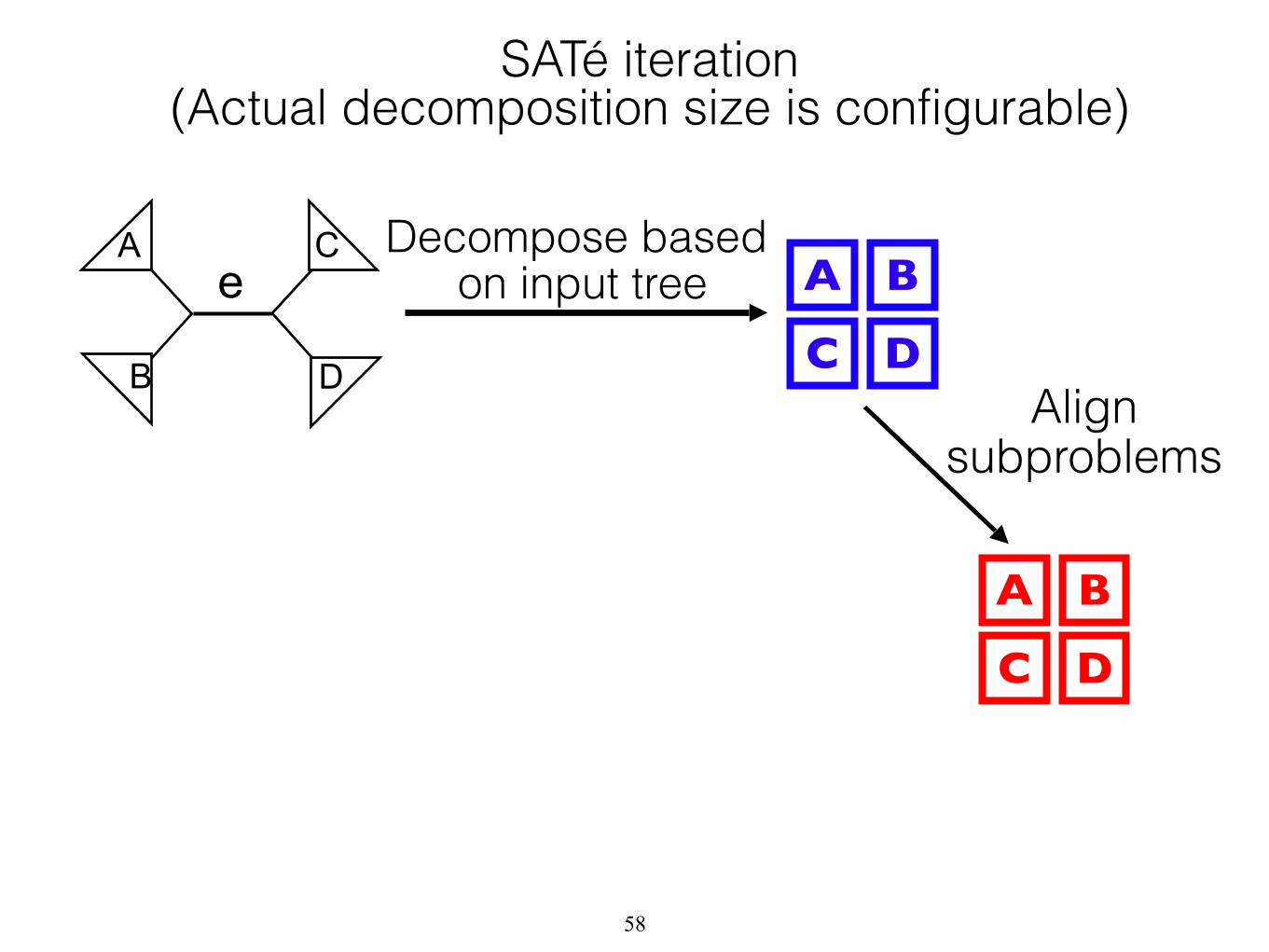
SATé iteration (Actual decomposition size is configurable)
57
A
B D
C Decompose based on input tree A B
C DAlign
subproblems
A B
C D
e
SATé iteration (Actual decomposition size is configurable)
58

A
B D
C
Merge subproblems
Decompose based on input tree A B
C DAlign
subproblems
A B
C D
ABCD
e
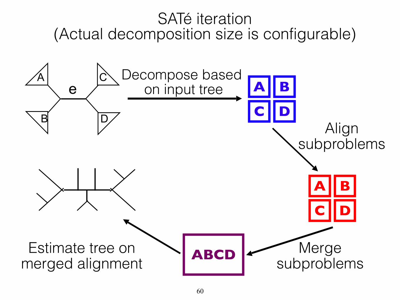
SATé iteration (Actual decomposition size is configurable)
59
A
B D
C
Merge subproblems
Estimate tree on merged alignment
Decompose based on input tree A B
C DAlign
subproblems
A B
C D
ABCD
e
SATé iteration (Actual decomposition size is configurable)
60
A
B D
C
Merge subproblems
Estimate tree on merged alignment
Decompose based on input tree A B
C DAlign
subproblems
A B
C D
ABCD
e
SATé iteration (Actual decomposition size is configurable)
61

Results on a Dataset with 27,000 Sequences
62Liu et al. Systematic Biology 2012.

Summary of Part I• Created novel tree-based divide-and-conquer
techniques for simultaneous alignment and tree estimation, enabling: - Scalability to thousands of sequences or more - High accuracy
• Family of algorithms included: - SATé (Liu et al. Science 2009) - SATé-II (Liu et al. Systematic Biology 2012) - and others
63

A Phylogeny, or Evolutionary Tree
Orangutan Gorilla Chimpanzee Human
Images from the Tree of the Life Website, University of Arizona, and Wikimedia

Evolutionary History● Phylogenetics is the
study of evolutionary history
● Helps us: − Predict gene function − Develop drugs and
vaccines − Understand disease
epidemics − Study the Tree of Life − Etc.
Source: www.tolweb.org
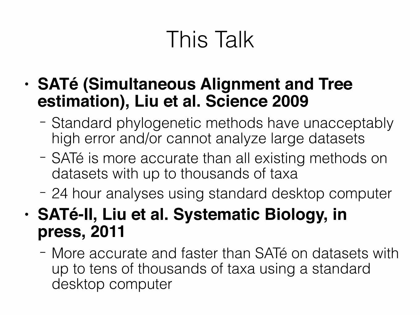
This Talk● SATé (Simultaneous Alignment and Tree
estimation), Liu et al. Science 2009!− Standard phylogenetic methods have unacceptably
high error and/or cannot analyze large datasets − SATé is more accurate than all existing methods on
datasets with up to thousands of taxa − 24 hour analyses using standard desktop computer
● SATé-II, Liu et al. Systematic Biology, in press, 2011!− More accurate and faster than SATé on datasets with
up to tens of thousands of taxa using a standard desktop computer

Many Trees and Many Alignments
67
● Number of trees |T| grows exponentially in n, the number of leaves: !
● The number of alignments |A| also grows exponentially in n and , where kj is the sequence length of the jth sequence (Slowinski MPE 1998): !
!
!
● NP-hard optimization problems

Counting Alignments
68

Two-phase Methodsu = -AGGCTATCACCTGACCTCCA v = TAG-CTATCAC--GACCGC-- w = TAG-CT-------GACCGC-- x = -------TCAC--GACCGACA
u = AGGCTATCACCTGACCTCCA v = TAGCTATCACGACCGC w = TAGCTGACCGC x = TCACGACCGACA
u
x
v
w
Phase 1: Align
Phase 2: Estimate Tree

Many Methods
Alignment method!• ClustalW!• MAFFT!• Muscle!• Prank!• Opal • Probcons (and Probtree) • Di-align • T-Coffee • Etc.

Many Methods
Alignment method!• ClustalW!• MAFFT!• Muscle!• Prank!• Opal • Probcons (and Probtree) • Di-align • T-Coffee • Etc.
Phylogeny method!• Maximum likelihood (ML)!
− RAxML!• Bayesian MCMC • Maximum parsimony • Neighbor joining • UPGMA • Quartet puzzling • Etc.

Simulation Study (Liu et al. Science 2009)
Simulation using ROSE ● Model trees with 1000 taxa ● Biologically realistic model with:
● Varied rates of substitutions ● Varied rates of insertions and deletions ● Varied gap length distribution − Long − Medium − Short

Tree Error
u
v
wx
y
FN
True Tree Estimated Tree
u
v
wx
y
● False Negative (FN): an edge in the true tree that is missing from the estimated tree
● Missing branch rate: the percentage of edges present in the true tree but missing from the estimated tree

Alignment Error
● False Negative (FN): pair of nucleotides present in true alignment but missing from estimated alignment
● Alignment SP-FN error: percentage of paired nucleotides present in true alignment but missing from estimated alignment
True Alignment Estimated Alignment
AACAT A-CCG
AACAT- A-CC-G
FN

1000 taxon models ranked by difficulty
Results
Problem with Two-phase Approach
● Problem: two-phase methods fail to return reasonable alignments and accurate trees on large and divergent datasets − manual alignment − unreliable alignments excluded from phylogenetic
analysis

u = CTATCACCTGACCTCCA v = CTATCACGACCGC w = CTGACCGC x = CGACCGACA
u = CTATCACCTGACCTCCA v = CTATCAC--GACCGC-- w = CT-------GACCGC-- x = ---TCAC--GACCGACA
and
u
x
v
w
Simultaneous Estimation of a Tree and Alignment

Existing Methods for Alignment and Tree Inference
• Two-phase methods - Infer an alignment, then use the alignment to infer a
tree - Inaccurate on data sets with thousands of
sequences • Methods based on statistical models
- Limited to datasets with a few hundred taxa - Unknown accuracy on larger datasets
• Parsimony-based methods - Slower than two-phase methods - No more accurate than two-phase methods

1000 taxon models ranked by difficulty
Results

Problem with Two-phase Approach
● Problem: two-phase methods fail to return reasonable alignments and accurate trees on large and divergent datasets
● Insight: divide-and-conquer to constrain dataset divergence and size
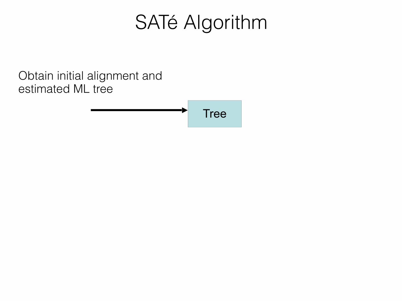
SATé Algorithm
Tree
Obtain initial alignment and estimated ML tree
SATé Algorithm
Tree
Obtain initial alignment and estimated ML tree
Insight: Use tree to perform divide-and-conquer alignmentAlignment

SATé Algorithm
Estimate ML tree on new alignment
Tree
Obtain initial alignment and estimated ML tree
Insight: Use tree to perform divide-and-conquer alignmentAlignment

Results
1000 taxon models ranked by difficulty

1000 taxon models ranked by difficulty
Results

● Problem: sometimes, subproblems have too many taxa or too divergent
Improving Upon SATé

Improving Upon SATé
● Problem: sometimes, subproblems have too many taxa or too divergent
● Insight: recurse

Improving upon SATé (Example)

Improving upon SATé (Example)

Improving upon SATé (Example)

A
B D
C
Merge subproblems
Estimate ML tree on merged alignment
Decompose based on input tree A B
C DAlign
subproblems
A B
C D
ABCD
e
Insight: recurse

1000 taxon models ranked by difficulty
Results

Num
ber o
f seq
uenc
es
Single gene Entire genome or a few genes
Less than1000
1000+
Graduate work:SATé,
SATé-II,DACTAL,
etc.
Postgraduate work:PhyloNet-HMM,
etc.
Sequence length
Outline for Today’s Talk
HPC Challenges• Email from UTCS IT staff. I had the most
computations by several orders of magnitude of any user at UTCS.
• If you let me, I’ll come and take over your clusters too.
• In all seriousness, my research has some fantastic low-hanging fruit for HPC contributions, particularly regarding parallel algorithms. <point to HPC researchers in the room>
94

Song et al. 2011. Images adapted from
Dejager et al. 2009 and the Jackson
Laboratory.
Different mouse species carrying warfarin
resistance gene
House mouse lacking warfarin resistance gene
Hybrid mouse carrying
warfarin resistance gene
Hybridization

Introgression
Approximately half of genome from A and half of genome from B
Species A Species B
First generation hybrid
96

IntrogressionSpecies A Species B
First generation hybridSpecies A
Introgressed hybrid
More than half of genome from A and less than half of genome from B
97

IntrogressionSpecies A Species B
First generation hybridSpecies A
Introgressed hybridSpecies A
...98

Naïve Sliding Windows
1. Break the genome into segments using a sliding-window (or other approaches)
2. Estimate a local tree in between every pair of breakpoints
99

Sliding Windows (Example)

Sliding Windows (Example)

Sliding Windows (Example)

Sliding Windows (Example)

Sliding Windows (Example)

Sliding Windows (Example)

Gene trees!(all identical)
Sliding Windows (Example)

107
A Gene Tree in a Species Tree (Example)
Species tree

108
A Gene Tree in a Species Tree (Example)
Species tree
Gene tree

Sliding Windows (Example)

Sliding Windows (Example)

Sliding Windows (Example)

Sliding Windows (Example)

Gene tree!incongruence!
Sliding Windows (Example)

114
“Horizontal” Gene Tree Incongruence (Example)
Species !network

115
“Horizontal” Gene Tree Incongruence (Example)
Gene trees
Species !network

Sliding Windows: Results
116Liu et al. in prep.

Sliding Windows Approach Is Too Simplistic
• Gene tree incongruence can occur for reasons other than introgression
• The organisms in our study included “vertical” gene tree incongruence due to: - Incomplete lineage sorting - Recombination
117
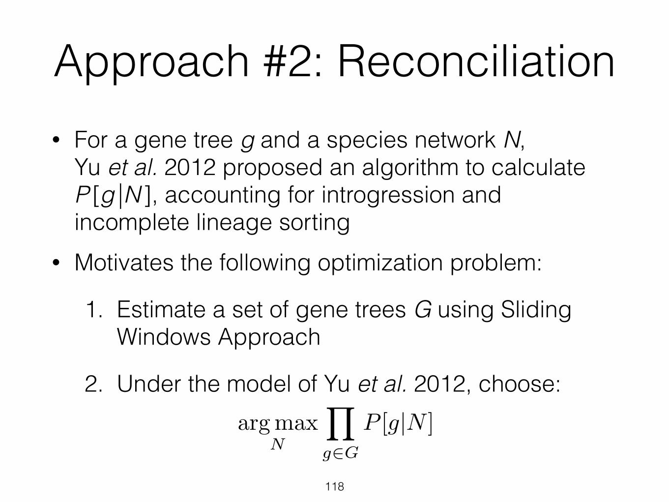
Approach #2: Reconciliation• For a gene tree g and a species network N,
Yu et al. 2012 proposed an algorithm to calculate P [g|N ], accounting for introgression and incomplete lineage sorting
• Motivates the following optimization problem:
1. Estimate a set of gene trees G using Sliding Windows Approach
2. Under the model of Yu et al. 2012, choose:
118

Approach #2: Reconcile Gene Trees with Species Network
• Relevant prior theoretical work: - Degnan and Salter 2005
• Probability P [g|T ] of observing a gene tree g given a species tree T
• Accounts for incomplete lineage sorting only - Yu et al. 2012
• Probability P [g|N ] of observing a gene tree g given a species network N
• Accounts for introgression and incomplete lineage sorting
119

Issues with Reconciliation-based Approaches
• Assumes that gene trees are correct - Estimated gene trees typically contain some error
• Assumes that each genome position is identically and independently distributed - Biologically unrealistic since adjacent
nucleotides tend to be inherited together • Doesn’t capture recombination
120

Problem: Computational Introgression
Detection
Input:
Species Genome ID Introgressed?A x UnknownA a No… … …A a NoB b No… … …B b No

Problem: Computational Introgression
Detection
Species Genome ID Introgressed?A x UnknownA a No… … …A a NoB b No… … …B b No
Input:
Output:
123
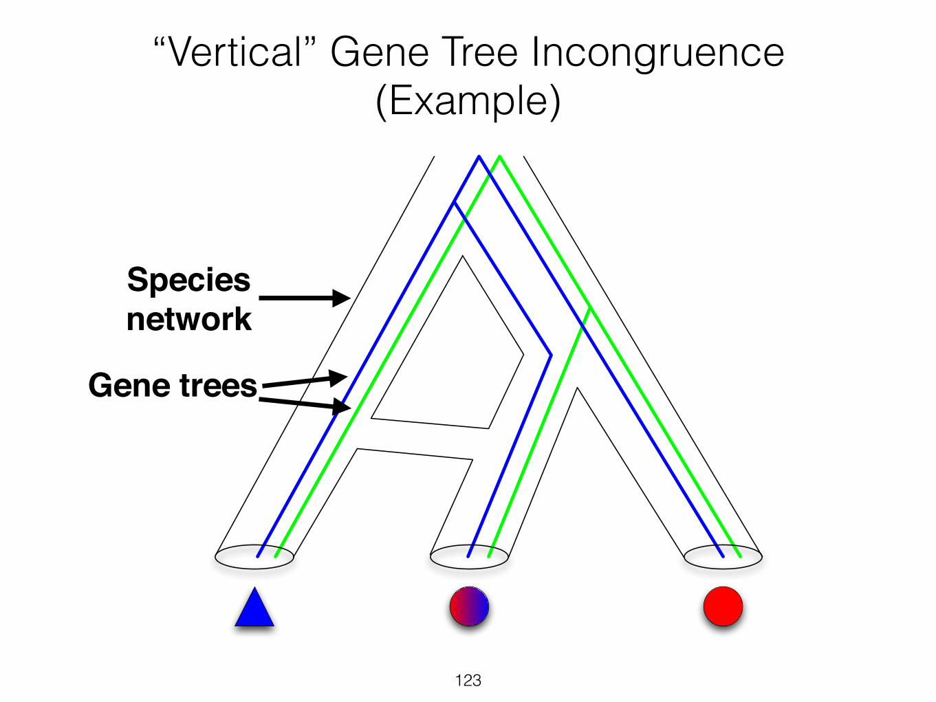
“Vertical” Gene Tree Incongruence (Example)
Gene trees
Species !network

124
“Horizontal” Gene Tree Incongruence (Example)
Gene trees
Species !network

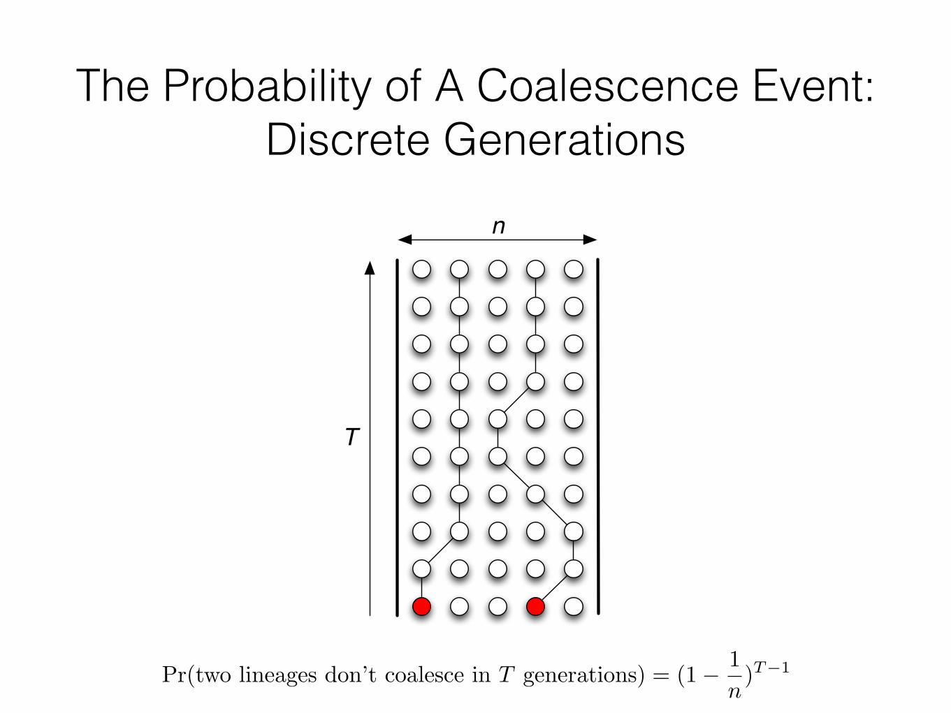
The Probability of A Coalescence Event: Discrete Generations
n
125

n
T
The Probability of A Coalescence Event: Discrete Generations
126

n
T
The Probability of A Coalescence Event: Discrete Generations

n
T
The Probability of A Coalescence Event: Discrete Generations
128
n
T
The Probability of A Coalescence Event: Discrete Generations

e T
n
The Probability of a Gene Tree in a Species Tree: Discrete Generations
130

g1 g2 g3f1
e T
The Probability of a Gene Tree in a Species Tree: Discrete Generations
131

g1 g2 g3f1
e T
The Probability of a Gene Tree in a Species Tree: Discrete Generations
132

g1 g2 g3f1
e T
133
The Probability of a Gene Tree in a Species Tree

• The probability of u lineages coalescing into v lineages in time T (Rosenberg 2002 and others):
!
!
• The probability of a gene tree topology g given a containing species tree (Ψ,λ) (Degan and Salter 2005):
134
25GENE TREE DISTRIBUTIONS
FIG. 1. (a,b) The species tree and gene tree, respectively, for the seven-taxon example, with internal nodes (equivalently, internalbranches) labeled according to a postorder traversal (Rosen 1999) so that no node has a lower number than any of its descendants. (c)Another representation of the species tree. The bifurcation points (upside-down v’s), which are pointed to by the dotted lines in (c),correspond to the nodes of the tree in (a). Note that (a) and (c) are drawn to the same scale, so that the branch lengths of (a) are thesame as the distances between the corresponding nodes of (c). (d) The gene tree with the branch lengths changed and curved so that itcan be superimposed on the species tree (c) to produce Figure 2a.
G. (See Fig. 2 for several scenarios in which this occurs.)Therefore, even though B and C share a recent ancestralpopulation, the B and C lineages for the gene of interest areonly related by a much more ancient ancestral population.Because this population must be at least as ancient as theroot, it must be ancestral both to the ((DF)(EG)) clade (withwhich C has coalesced) and to A (with which B has coa-lesced). In this case, lineage sorting causes the gene tree andspecies tree to have different topologies. Because differentgenes can have separate evolutionary histories, there is no apriori reason to expect that gene trees based on different genesshould have the same topologies. By sufficiently changingthe branch lengths (and, for graphical purposes, allowing thebranches to bend), any gene tree can be made to fit withinany species tree (Fig. 1d). To see that this is always true,note that there is always the possibility that none of the genelineages coalesce more recently than the root of the speciestree. If all lineages coalesce prior to the root, then the lineagescan coalesce in any order, thereby producing any desiredtopology for the gene tree. As will be seen below, however,gene trees with topologies radically different from that of thespecies tree tend to have very low probabilities.Coalescent theory, which models coalescent times for a
set of lineages, can be used to calculate the probability thattwo or more lineages coalesce within a fixed amount time.By treating the species tree (including branch lengths) asfixed, one can calculate the probability that, for instance, twolineages coalesce into one, or more generally that u lineagescoalesce into v lineages, within the amount of time deter-mined by the length of the branch. This probability can thenbe expressed as puv(T), where T is the length of the branch.
Here u $ v $ 1, and if u 5 v, then puv(T) is the probabilitythat no coalescences occur in the length of time T. In thecoalescent model, T 5 t/(2N), where t is the number of gen-erations and N is the effective population size—the numberof diploid individuals—which is assumed to be constant (Ta-jima 1983; Takahata and Nei 1985). An expression for thisprobability was given by Rosenberg (2002) and was derivedearlier by several others (Tavare 1984; Watterson 1984; Tak-ahata and Nei 1985):
u k2v(2k 2 1)(21)2k(k21)T/2p (T ) 5 eOuv v!(k 2 v)!(v 1 k 2 1)k5v
k21 (v 1 y)(u 2 y)3 . (1)P (u 1 y)y50
By counting the number of ways that a gene tree couldhave arisen on the species tree and determining the puv(T)term for each branch, one can calculate the probability of agene tree for a fixed species tree. This is feasible to do byhand for small trees (e.g., fewer than six taxa). For largertrees, the notation and concepts that follow can be used todevelop an algorithm for the computation.This method requires keeping track of lineages from a gene
tree coalescing on branches of the species tree. The internalnodes of the trees are labeled according to a postorder tra-versal (Rosen 1999; Fig. 1). The terms ‘‘node’’ and ‘‘clade’’are used interchangeably, so that, for example, the clade((DE)(FG)) of the species tree in Figure 1a is called eithernode 5 or clade 5. In addition, each branch has the numberof the node incident to that branch and closer to the tips ofthe tree. For example, branch 5 of the species tree is the
28 J. H. DEGNAN AND L. A. SALTER
from the probability of the events on each branch, using thepuv(T) terms from equation (1). Here the probability that ulineages coalesce into v lineages on a specific branch mustalso reflect the possibility that there might be more than oneway for these coalescences to occur. Assuming that all pos-sible orderings, correct and incorrect, are equally likely (thisfollows the model of Yule [1924]), and that u lineages havecoalesced into v lineages, the probability that the ordering ofevents on the branch is consistent with the gene tree is thenumber of correct orderings divided by the number of pos-sible orderings. Multiplying the probabilities of the eventson different branches yields the probability of the coalescenthistory for the entire tree. (These probabilities are not nec-essarily independent because they depend on the events ofdescendent branches. This will be discussed below.) Givena list of coalescent histories and the probabilities of eventson each branch, the overall probability of a gene tree givena species tree can be obtained.Under the coalescent model, for a given n-taxon species
tree with topology c and vector of branch lengths l 5 (l1,l2, . . . , ln22), where each lb is measured in units of 2Ngenerations, the gene tree topology G is a random variablewith probability mass function
n22w(h) w (h)bP (G 5 g) 5 p (l ). (2)O Pc,l u (h)v (h) bb bd(h) d (h)h∈H (g) b51 bc
The sum is over all histories h taken from the set Hc(g) ofall valid coalescent histories for the particular gene tree andspecies tree. The product is taken over all internal branchesof the species tree, labeled 1, 2, . . . , n 2 2. The terms
, which can be determined from equation (1), arep (l )u (h)v (h) bb bused to calculate the probability, for a particular coalescenthistory h and a particular branch b, that ub(h) lineages co-alesce into vb(h) lineages in the time lb, the length of branchb. Here 2 # ub(h) # db, where db is the number of taxa forwhich branch b is an ancestor, and 1 # vb(h) # ub(h). Theterms wb(h)/db(h) and w(h)/d(h) determine the probabilityfor each branch and prior to the root that the coalescent eventsare consistent with the gene tree. Here wb(h) is the numberof ways that coalescent events on a branch can occur con-sistently with the gene tree, and db(h) is the number of pos-sible orderings of events.The next two sections provide details for enumerating co-
alescent histories and for computing the necessary terms inequation (2), and can be skipped without loss of continuity.These are followed by discussions regarding the shape ofgene tree distributions, the number of coalescent histories,applications, and possible extensions.
ENUMERATING COALESCENT HISTORIES
To enumerate the set of valid coalescent histories Hc(g),each proposed coalescent history h can be identified with aninteger h 5 (hk 2 1) (n 2 1)n222k. The values of h aren22Ok51at most (n 2 1)n22 2 1, which corresponds to the coalescenthistory h 5 (n 2 1, n 2 1, . . . , n 2 1). This value of hoccurs when all clades of the gene tree coalesce prior to theroot. If a proposed history h is valid, then h ∈ Hc(g). Theproblem of determining the set of valid coalescent histories
is to enumerate values of h for which 0 # h # (n 2 1)n22
2 1 and that correspond to valid histories.To check whether a proposed coalescent history h 5 (h1,
h2, . . . , hn22) is valid, it must be the case that if hk 5 b, thatis, if clade k of the gene tree coalesces on branch b of thespecies tree, then all of the taxa in clade kmust be descendantsof branch b on the species tree. These restrictions on validcoalescent histories can be summarized in a matrixM5 (mij),where mij 5 1 if clade j of the gene tree only includes taxathat are also in clade i of the species tree; otherwise, mij 50. Therefore, a necessary condition for a coalescent historyh 5 (h1, h2, . . . , hn22) to be valid is that if hk 5 b, and if b# n 2 2, then mbk 5 1 for all k 5 1, 2, . . . , n 2 2. Notethat any clade of the gene tree can coalesce prior to the rootof the species tree, and that the clade associated with the rootof the gene tree can only coalesce prior to the root of thespecies tree. Consequently, we only need to keep track ofclades 1, 2, . . . , n 2 2 of the gene tree and branches 1, 2,. . . , n 2 2 of the species tree, so the M matrix is (n 2 2)3 (n 2 2).For even a moderate number of taxa, the maximum value
of h, (n 2 1)n22 2 1, is unmanageably large. To reduce thenumber of histories that must be evaluated, h can be incre-mented more rapidly by skipping over large numbers of con-secutively occurring histories that are not allowed. In par-ticular, if the proposed coalescent history has the form h 5(h1, h2, . . . , hk, 1, . . . , 1) with hk 5 b . 1 and mbk 5 0,then that history is prohibited by the M matrix, as are allremaining vectors that have hk 5 b. If the proposed historiesare enumerated sequentially, then the next (n 2 1)n222k 2 1histories are invalid, and therefore do not need to be checked.This greatly reduces the number of histories that must beevaluated.As an example of filling in the M matrix for Figures 1a
and 1b, consider m52. Because all taxa in clade 2 of the genetree are present in clade 5 of the species tree, a valid coa-lescent history might have clade 2 of the gene tree coalesceon branch 5 of the species tree. Therefore, m52 5 1. Fillingin the matrix yields
0 0 0 0 0
1 0 0 0 0 M 5 0 0 0 0 0 . (3)
0 0 0 0 0 0 1 1 1 0
Recalling that any clade can coalesce prior to the root (i.e.,branch 6), this M matrix specifies that clade 1 can only co-alesce on branch 2 or 6; clades 2, 3, and 4 can only coalesceon branch 5 or 6; and clade 5 can only coalesce prior to theroot.A further restriction for a coalescent history h to be valid
is that if i and j are clades of the gene tree and j is an ancestorof i, then i must coalesce more recently than j or on the samebranch of the species tree as j. Again, these restrictions canbe represented as a matrix R 5 (rij) where rij 5 1 if and onlyif i is an ancestor of j on the gene tree; otherwise, rij 5 0.A coalescent history h 5 (h1, . . . , hi, . . . , hj, . . . , hn22),with 1 # i , j # n 2 2, is not permissible if hj , hi and j
The Probability of a Gene Tree in a Species Tree

PhyloNet-HMM• Each hidden state si is associated with a gene tree g(si)
contained within a “parental” tree f(si)
• The set of HMM parameters λ consists of
- The initial state distribution π
- Transition probabilities
where γ is the “horizontal” parental tree switching frequency.
- The emission probabilities bi = P(Ot|g(si))
135

• Each hidden state si is associated with a gene tree g(si) contained within a “parental” tree f(si).
• Let qt be PhyloNet-HMM’s hidden state at time t, where 1≤t≤k and k is the length of the input observation sequence O.
• The set of HMM parameters λ consists of:
- Transition probabilities A={aij}, where
and γ is the “vertical” parental tree switching frequency and Pr[g(s
- The emission probabilities bi = Pr[Ot|g(si)] under a model of nucleotide substitution (e.g., Jukes-Cantor (1969))
- The initial state distribution πi = P[q1 = si]
136
PhyloNet-HMMq1 q2 q3
r1 r2 r3
s0
Introgressed
Non-introgressed

• Let qt be PhyloNet-HMM’s hidden state at time t, where 1≤t≤k and k is the length of the input observation sequence O.
• What is the likelihood of the model given the observed DNA sequences O?
- Forward algorithm calculates “prefix” probability
- Backward algorithm calculates “suffix” probability
- Model likelihood is
137
First HMM-related Problem
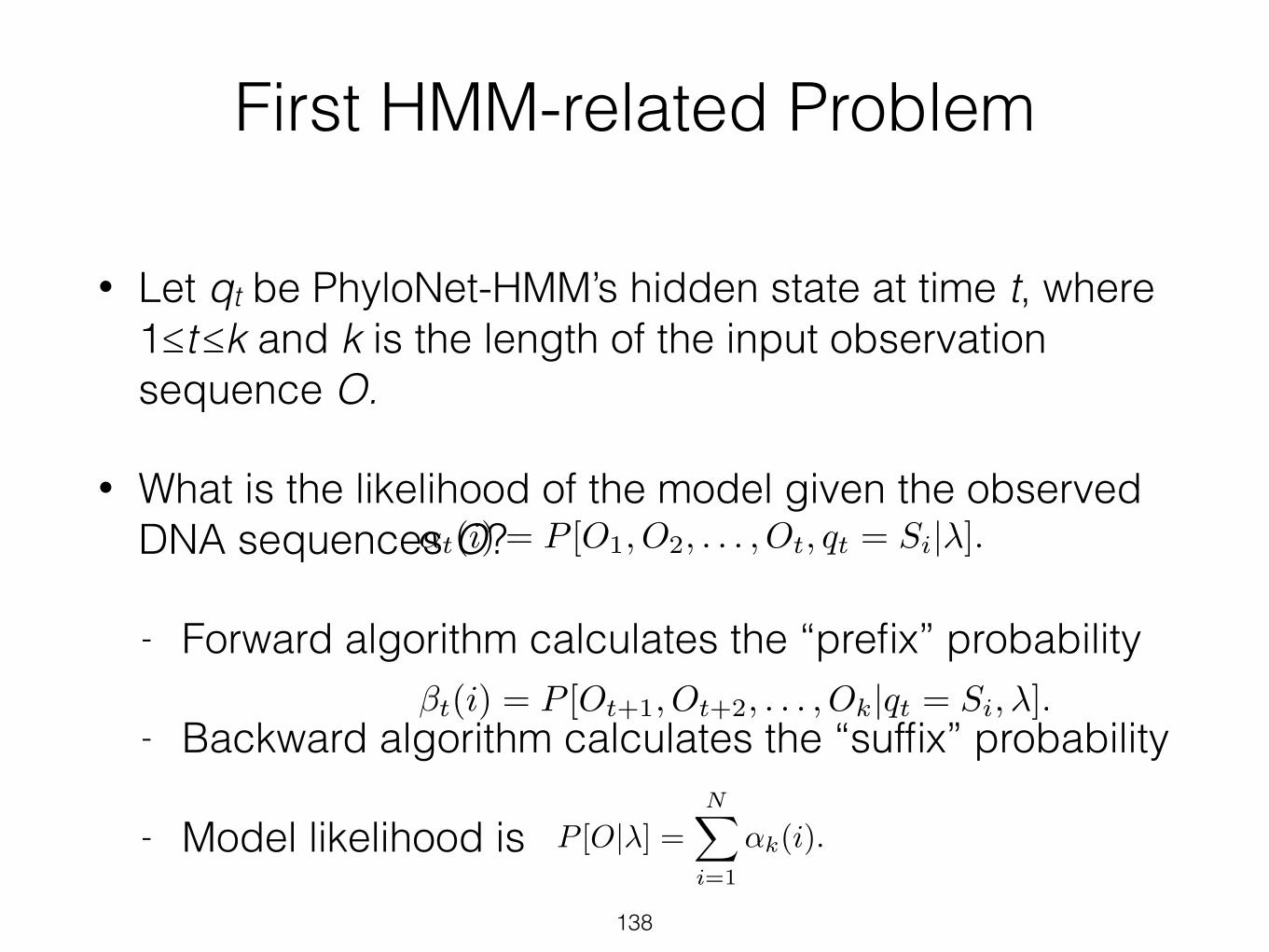
• Let qt be PhyloNet-HMM’s hidden state at time t, where 1≤t≤k and k is the length of the input observation sequence O.
• What is the likelihood of the model given the observed DNA sequences O?
- Forward algorithm calculates the “prefix” probability
- Backward algorithm calculates the “suffix” probability
- Model likelihood is
138
First HMM-related Problem

• Which sequence of states best explains the observation sequence?
- Posterior decoding probability γt(i) is the probability that the HMM is in state si at time t, which can be computed as:
139
Second HMM-related Problem

• How do we choose parameter values that maximize the model likelihood?
- Perform local search to optimize the criterion
140
Third HMM-related Problem

Related HMM-based Approaches
• CoalHMM (Mailund et al. 2012) - Models introgression + incomplete lineage
sorting + recombination (with a simplifying assumption)
- Currently supports two sequences only - Assumes that time is discretized
• Other approaches that don’t account for introgression (e.g., Hobolth et al. 2007)
141

Simulation Study Results
142
0 2 4 6 8
10 12 14
0 0.4 0.8
Perc
enta
ge o
f site
s w
ithin
ferre
d ho
rizon
tal g
ene
flow
Horizontal gene flow rate M
tm1=0.015 tm2=0.15tm1=0.015 tm2=0.3

143
14
infers no introgression for any of the sites. For the isolation-with migration models (M > 0),the inferred percentages of introgressed sites were greater than zero and increased as a functionof the migration rate M . A potentially more informative comparison would be between theinferred percentages of introgressed sites and the percentages of sites in the simulation thatinvolved migrant lineages. However, the simulation software that we used does not supportannotating lineages in this way, nor is it a simple task to modify it to achieve this goal.
Clearly, when the duration of the migration period increases (corresponds to the red curvein the figure), the variation in the estimates of our method increases, which results in a patternthat seemingly does not change from migration rate 0.4 to 0.8. However, it is important to notethat the extent of variability in this case precludes making a conclusion on the lack of increasein the percentage of sites. Nonetheless, the important message here is that the estimates of ourmethod start varying more as the duration of the migration period increases.
We also found that the probability of observing a gene genealogy conditional on a containingparental tree di↵ered between the two parental trees (results not shown). Under all simulationconditions, the inferred gene tree distribution (conditional on the containing parental tree) hadmultiple genealogies with non-trivial posterior decoding probabilities, suggesting that within-row transitions were capturing switching in local genealogies due to ILS. That is, the simulateddata sets clearly had evidence of incongruence due to both introgression and ILS.
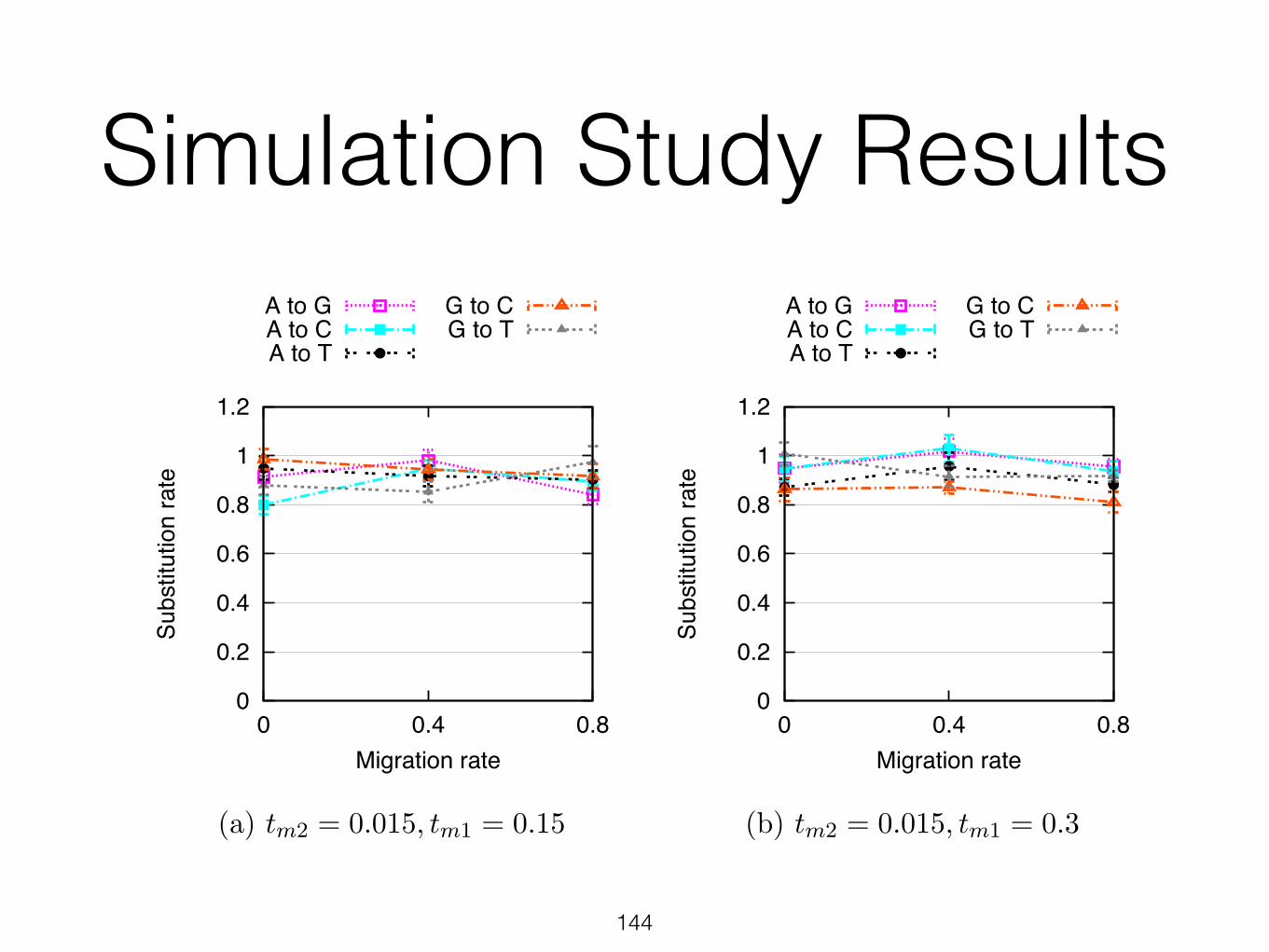
Finally, Fig. 7 and Fig. 8 show that in training our PhyloNet-HMM model on the simulateddata, base frequencies were accurately estimated at 0.25 (which are the base frequencies for allfour nucleotides we used in our simulations) and substitution rates were estimated generallybetween 0.8 and 1 (we used 1 in our simulations). Further, the results were robust to themigration rates and durations of migration periods.
0 0.05 0.1
0.15 0.2
0.25 0.3
0 0.4 0.8
Freq
uenc
y
Migration rate
0 0.05 0.1
0.15 0.2
0.25 0.3
0 0.4 0.8
Freq
uenc
yMigration rate
(a) tm2 = 0.015, t
m1 = 0.15 (b) tm2 = 0.015, t
m1 = 0.3
Figure 7. Empirical base frequencies inferred by PhyloNet-HMM on simulated data sets.Panels (a) and (b) show model conditions with migration times tm2 = 0.015, tm1 = 0.15 andtm2 = 0.015, tm1 = 0.3, respectively, and di↵erent migration rates. Standard error bars are shown, andn = 20.
Simulation Study Results
144
15
0
0.2
0.4
0.6
0.8
1
1.2
0 0.4 0.8
Subs
titut
ion
rate
Migration rate
A to GA to CA to T
G to CG to T
0
0.2
0.4
0.6
0.8
1
1.2
0 0.4 0.8Su
bstit
utio
n ra
te
Migration rate
A to GA to CA to T
G to CG to T
(a) tm2 = 0.015, t
m1 = 0.15 (b) tm2 = 0.015, t
m1 = 0.3
Figure 8. Empirical substitution rates inferred by PhyloNet-HMM on simulated datasets. Otherwise, figure layout and description match Figure 7.
Empirical study
We applied the PhyloNet-HMM framework to detect introgression in chromosome 7 in three setsof mice, as described above. Each data set consisted of two individuals from M. m. domesticusand two individuals from M. spretus. Thus the phylogenetic network is very simple, and hasonly two leaves, with a reticulation edge from M. spretus to M. m. domesticus; see Fig. 9(a).As we discussed above, the evolution of lineages within the species network can be equivalently
M. m. domesticus M. spretus
t1
t2γ
M.m.d M.s. M.m.d M.s.M.m.d
(a) (b) (c)
Figure 9. The phylogenetic network used in our analyses and the two parental trees. Thephylogenetic network (a) captures introgression from M. spretus to M. m. domesticus. The red and bluelines illustrate two possible gene genealogies involving no introgression (blue) and introgression (red).The parental tree in (b) captures genomic regions with no introgression, while the parental tree in (c)captures genomic regions of introgressive descent.
captured by the set of parental trees in Fig. 9(b-c). Since in each data set we have four genomes,there are 15 possible rooted gene trees on four taxa. Therefore, for each data set, our modelconsisted of 15 q states, 15 r states, and one start state s0, for a total of 31 states.
We use our new model and inference method to analyze two types of empirical data sets.
Simulation Study Results

145
Figure 1: Adaptive introgression scans of chromosome 7 from the Spanish-domesticussample. PhyloNet-HMM was used to scan the chromosome (21). The Spanish-domesticussample came from the region of sympatry between M. m. domesticus and M. spretus. (a)The posterior decoding probability that a genomic segment has introgressed origin from M.spretus. (b) For introgressed genomic segments, the posterior decoding probability of eachrooted gene genealogy is shown for each locus using a heatmap. Each of the 15 possible rootedgene genealogies is shown in a different track. A block in a track is shaded according to theprobability of observing the rooted gene genealogy in the corresponding genomic segment,where shades are a continuous gradient from white to blue corresponding to probabilities from0 to 1. (continued on next page)
8

146
0 0.25 0.5
0.75 1
Prob
abilit
y
(a)
Intro−
gres
sed
Gen
e ge
neal
ogie
s
0 0.2 0.4 0.6 0.8 1Probability
(b)
Non−
intro−
gres
sed (c)
0 50 100 150 200Position along chromosome (Mb)
(d)
Figure S24: Results from PhyloNet-HMM scan of chromosome 7 from the M. m. musculuscontrol data set. Figure layout and description are otherwise identical to Figure 1 panels a-c andf.
40

147
0 0.25 0.5
0.75 1
Prob
abilit
y
(a)In
tro−
gres
sed
Gen
e ge
neal
ogie
s
0 0.2 0.4 0.6 0.8 1Probability
(b)
Non−
intro−
gres
sed (c)
0 50 100 150 200Position along chromosome (Mb)
(d)
Figure S23: Results from PhyloNet-HMM scan of chromosome 7 from the reference straincontrol data set. Figure layout and description are otherwise identical to Figure 1 panels a-c andf.
39

148
PhyloNet-HMM Scan of Whole Mouse Genomes
0
2
4
6
8
10
Perc
enta
ge w
ithin
trogr
esse
dor
igin
(%)
(a)
0
2
4
6
8
10
17 7 12 6 1 8 11 2 3 4 5 9 10 13 14 15 16 18 19
Tota
l len
gth
with
intro
gres
sed
orig
in (M
b)
Chromosome
(b)
Liu et al. in prep. for PNAS.

Future Direction #4
• Measures of selection under complex evolutionary scenarios.
149

DNA Sequence Evolution
• Walk through calculation on a single edge.
• Then for a three taxon tree.
150

Future Direction #1
151
S1 S2 S3 S4 S5

Future Direction #1
152
S1 S2 S3 S4 S5

Future Direction #2
• The most widely used multiple sequence alignment methods assume that evolution is tree-like.
153
AAGACTT
AAGGCTT AAGACTT
TAGCCCA TAGACTT AGCGAGCAATCGGGCAT
ATCGGGCAT TAGCCCT A
Substitutions Insertions Deletions

Future Direction #2
• The most widely used multiple sequence alignment methods assume that evolution is tree-like.
• I propose to extend alignment approaches to the case where evolution is not tree-like.
154
AAGACTT
AAGGCTT AAGACTT
AAGTAGCCC AAGTAGACT AGCGAGCAATCGGGCAT
ATCGGGCAT AAGTAGCCCT A
Substitutions Insertions Deletions

Warfarin-‐associated Genes with Introgressed Origin
Visualized using Cytoscape (www.cytoscape.org).
• Each pink node is a gene.
• Each blue link is an interaction between a pair of genes.
155

Visualized using Cytoscape (www.cytoscape.org).
Vkorc1 gene
Warfarin-‐associated Genes with Introgressed Origin
156

Visualized using Cytoscape (www.cytoscape.org).
Vkorc1 geneCytochrome P450
genes (highly studied,
responsible for drug metabolism)
Warfarin-‐associated Genes with Introgressed Origin = New Potential Targets for Personalized Warfarin Therapy
157

Visualized using Cytoscape (www.cytoscape.org).
Vkorc1 gene
Poorly understood “orphan”
cytochrome P450 gene
Warfarin-‐associated Genes with Introgressed Origin = New Potential Targets for Personalized Warfarin Therapy
Cytochrome P450 genes
(highly studied, responsible for drug
metabolism)
158

Acknowledgments
• Thanks to my postdoctoral mentors (Luay Nakhleh and Michael H. Kohn), my graduate adviser and co-‐adviser (Tandy Warnow and C. Randal Linder), and their labs.
• Supported in part by: –A training fellowship from the Keck Center of the Gulf Coast Consortia, on Rice University’s NLM Training Program in Biomedical Informatics (Grant No. T15LM007093).
–NLM (Grant No. R01LM00949405 to Luay Nakhleh) –NHLBI (Grant No. R01HL09100704 to Michael Kohn)
Introgression of Functional
Gene Modules
160Liu et al. in prep.

161
Introgression of a
Functional Cluster of Olfactory Receptor- Related Genes

Other • Computational approaches constitute basic research of interest
to NSF (IIS, ABI)
• Wide range of applications of interest to different funding agencies, including:
- The role of introgression in the spread of pesticide resistance in wild mice, with applications to personalized warfarin therapy (NIH)
- The role of horizontal gene transfer in the spread of antibiotic resistance in bacteria (NIH)
- Bacterial genomics (DOE)
- Hybridization in plants (USDA)
162

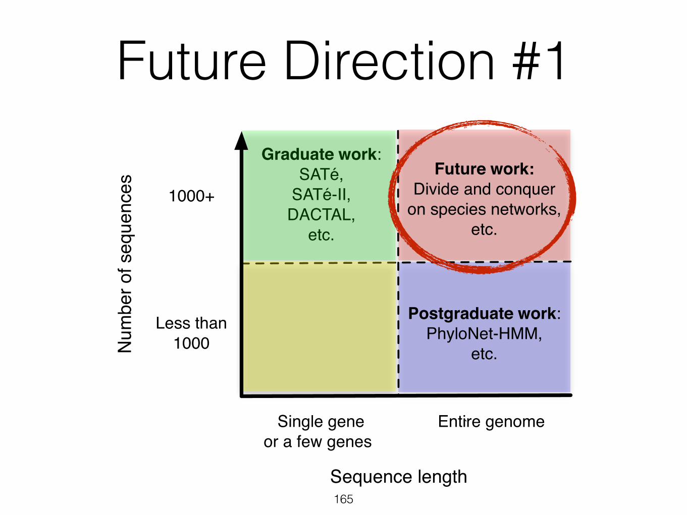
Future Direction #1• Previous analyses (at most five genomes and a
single network edge) required more than a CPU-month on a large cluster
• Problem is combinatorial in both the number of genomes and the number of network edges
• Challenge: efficient and accurate network-based inference from hundreds of genomes or more
163

My ContributionsN
umbe
r of s
eque
nces
Single gene Entire genome or a few genes
Less than1000
1000+
Graduate work:SATé,
SATé-II,DACTAL,
etc.
Postgraduate work:PhyloNet-HMM,
etc.
Sequence length
Num
ber o
f seq
uenc
es
Single gene Entire genome or a few genes
`
Less than1000
1000+
Graduate work:SATé,
SATé-II,DACTAL,
etc.
Postgraduate work:PhyloNet-HMM,
etc.
Future work:Divide and conquer
on species networks,etc.
Sequence length
Future Direction #1
165

Future Direction #2
Number
of seq
uences
Single gene Entire genomeor a few genes
`
Less than1000
1000+
Graduate work:SATé,
SATé-II,DACTAL,
etc.
Postgraduate work:PhyloNet-HMM,
etc.
Future work:Divide and conquer
on species networks
Sequence length
166

Future Direction #2
Number
of seq
uences
Single gene Entire genomeor a few genes
`
Less than1000
1000+
Graduate work:SATé,
SATé-II,DACTAL,
etc.
Postgraduate work:PhyloNet-HMM,
etc.
Future work:Divide and conquer
on species networks
Sequence length
"Syntax" ofGenomic
Information andArchitecture
167

Number
of seq
uences
Single gene Entire genomeor a few genes
`
Less than1000
1000+
Graduate work:SATé,
SATé-II,DACTAL,
etc.
Postgraduate work:PhyloNet-HMM,
etc.
Future work:Divide and conquer
on species networks
Sequence length
"Syntax" ofGenomic
Information andArchitecture
"Semantics" ofBiological
Function andSystemsBiology
Future Direction #2
168

Number
of seq
uences
Single gene Entire genomeor a few genes
`
Less than1000
1000+
Graduate work:SATé,
SATé-II,DACTAL,
etc.
Postgraduate work:PhyloNet-HMM,
etc.
Future work:Divide and conquer
on species networks
Sequence length
"Syntax" ofGenomic
Information andArchitecture
InteractomicData
GeneExpression
Data
Phenotypic(Trait)Data
"Semantics" ofBiological
Function andSystemsBiology
Future Direction #2
169