An Evaluation of Radio-Noise-Meter Performance

in Terms of Listening Experience*CHARLES M. BURRILLt, 1EMBER, I.R.E.

Summary-An account is given of listening tests conducted, withthe co-operation of the Joint Co-ordination Committee on Radio Re-ception of the Edison Electric Institute, National Electrical Manu-facturers Association, and Radio Manufacturers Association, for thepurpose of indicating how closely instruments made in accordancewith the latest radio-noise-meter specifications of the Joint Co-ordina-tion Committee meet the objective of giving readings proportional toannoyance for all types of radio noise. Thirty people participated inthe tests which involved three types of radio noise and three differentradio-noise meters. Standard statistical methods are used in analyzingthe results, and these methods are explained in simple fashion for thebenefit of radio engineers who are unfamiliar with statistical science.The general conclusion is that the new radio-noise-meter performance isvery satisfactory.

INTRODUCTIONA MAJOR objective of radio-noise-meter design

is to provide an instrument which will give, forall kinds of radio noise, indications which are

proportional to the annoyance factor or nuisancecapability of the noise. This annoyance factor mustultimately be determined by listening experience.Therefore, the performance of each new design shouldbe calibrated or evaluated by means of listening tests,in which the instrument readings are compared withthe judgments of a jury of listeners as to the vexatious-ness of the noises measured. The general problems in-volved in this basic procedure of radio-noise measure-ment have been discussed at length elsewhere.",2 Theprincipal purpose of the present paper is to describe aseries of tests which were made to evaluate, in terms oflistening experience, the performance of radio-noisemeters built in accordance with the latest specifica-tions of the Joint Co-ordination Committee on RadioReception of the Edison Electric Institute, NationalElectrical Manufacturers Association, and Radio Man-ufacturers Association.3 A further purpose is to ana-lyze and state the results of these tests in simple, easilyunderstood terms in conformance with standard statis-tical practice. The exposition will therefore serve toillustrate the application of statistical methods to aradio-engineering problem, and to suggest to radioengineers relatively unfamiliar with such methods howthey might be more widely used.The tests to be described were planned and carried

out, with the co-operation of the Joint Co-ordination* Decimal classification: R2 70. Original manuscript received by

the Institute, December 10, 1941. Presented, Annual Convention,New York, N. Y., January 9, 1941.

t RCA Manufacturing Co., Inc., Camden, N. J.' C. J. Franks, "The measurement of radio noise interference,"

RMA Eng., vol. 3, pp. 7-10; November, 1938.2 C. M. Burrill, "Progress in the development of instruments for

measuring radio noise," PROC. I.R.E., vol. 29, pp. 433-442; August,1941.

3 aMethods of measuring radio noise, a report of the Joint Co-ordination Committee on Radio Reception of the Edison ElectricInstitute, National Electrical Manufacturers Association, andRadio Manufacturers Association." Edison Electric Institute Pub-lication No. G9, National Electrical Manufacturers AssociationPublication No. 107, Radio Manufacturers Association EngineeringBulletin No. 32; February, 1940.

Committee, by Dudley E. Foster at the RCA LicenseLaboratory in New York City. Two manufacturers ofradio-noise meters loaned the instruments which wereused. The tests were held on the morning of May 24,1940, preceding a regular meeting of the Joint Co-ordination Committee, so that the committee mem-bers and their guests could form the jury of listeners.

THE RADIO-NOISE METERSThree instruments were used, designated A, B, and

C. A and B were of different manufacture but bothwere intended to be in accordance with the Joint Co-ordination Committee specifications.3 C was similarto A, but incorporated time constants of 1 and 160milliseconds, such as were being considered forstandardization in Canada, instead of the time con-stants of 10 and 600 milliseconds adopted by the JointCo-ordination Committee.

THE RADIO-NOISE SOURCESThe noise from a direct-current commutator-type

motor, that from an electric razor of the vibrator type,and the clicks from a direct-current relay were chosenfor use as typical of a large percentage of radio noisesencountered in broadcast reception. These noisesources covered the range from fairly continuous noiseto impulse noise of repetition rates as slow as aboutone per second.

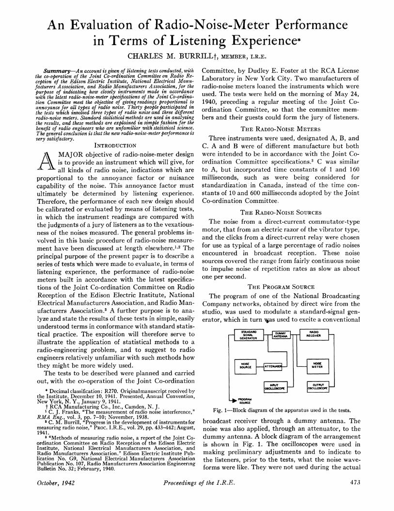
THE PROGRAM SOURCEThe program of one of the National Broadcasting

Company networks, obtained by direct wire from thestudio, was used to modulate a standard-signal gen-erator, which in turn 4as used to excite a conventional

L*SOURCE

Fig. 1-Block diagram of the apparatus used in the tests.

broadcast receiver through a dummy antenna. Thenoise was also applied, through an attenuator, to thedummy antenna. A block diagram of the arrangementis shown in Fig. 1. The oscilloscopes were used inmaking preliminary adjustments and to indicate tothe listeners, prior to the tests, what the noise wave-forms were like. They were not used during the actual

Proceedings of the I.R.E.

r

October, 1942 473

Proceedings of the I.R.E.

tests. Two different receivers were used, a 13-tubeconsole model and a 6-tube table model. The programwas taken just as it came: speech, music, announce-ments, and all.

QUALITY OF RECEPTION

The quality of the program reception, with respectto noise interference, was rated by each listener inaccordance with the following scale or code devisedby the author some time ago :'

A-Entirely satisfactoryB-Very good, background unobtrusiveC-Fairly satisfactory, background plainly evidentD-Background very evident, but speech easily

understoodE-Speech understandable only with severe con-

centrationF-Speech unintelligible

Intermediate grades were recognized, for example,B- was considered identical with C+ and half waybetween B and C.

This scale is a composite one, intended to be of usefor programs consisting of either speech or music,whether listened to for entertainment as, for example,symphonic music, or for intelligence as, for example,news broadcasts. It is recognized that there is someloss of precision in using a single scale for all typesof program. However, in the present state of the artof radio-noise measurement, the refinement of separateevaluations for different program types does not ap-pear to be warranted. In using the present scale it isfound that the three highest grades, A, B, and C aremore easily differentiated when grading a musical pro-gram, while grades D, E, and F are most significantwith respect to speech. Hence, if a given program sam-ple contains both speech and music, it is readilygraded, whatever its quality may happen to be.

SIGNAL-TO-NOISE RATIOS

The signal-to-noise ratio corresponding to each pro-gram sample or listening period was obtained beforethe period from the radio-noise-meter readings, firstwith the program-modulated carrier on and the noisestopped and then with the noise on but with the car-rier off. The ratio between these two readings is thesignal-to-noise ratio, which will be expressed in deci-bels in this paper. It was assumed that both signal andnoise remained at constant levels between the time ofmeasurement and the listening period. The noisesources were so chosen as to justify this assumptionwith respect to them. The program level was sensiblvconstant, as is usual with the type of program ordi-narily broadcast in the morning hours. Signal-to-noiseratios were determined for each program sample witheach of the three radio-noise meters.

4 C. M. Burrill, discussion of paper by C. V. Aggers, D. E.Foster, and C. S. Young, 'Instruments and methods of measuringradio noise," Elec. Eng., vol. 59, pp. 178-192; March, 1940.

THE TESTSEach of thirty observers, most of them untrained

in listening tests, graded the "quality of reception" oftwenty-four listening periods, comprising four dif-ferent signal-to-noise ratios with three different kindsof noise, reproduced on two different receivers. Thevarious signal-to-noise-ratio values were presented inrandom order, and the observers were not informedof these values until after the completion of all thegrading. Table I gives the order of the test periods,together with the corresponding signal-to-noise-ratiovalues as determined with each of the three radio-noise meters.

TABLE I

Noise-Meter Signal-to-NoiseTest sNoise Receiver Ratio-DecibelsTet Source Type

A B C

IA Commutator Console 28.9 28.5 33.2lB Commutator Console 19.2 19.7 25.0IC Commutator Console 45.8 45.4 50. 1ID Commutator Console 54.8 54.4 59.1

2A Razor Console 40.6 40.6 50.12 B Razor Console 14.6 12.6 19.22C Razor Console 48.6 48.6 58.12D Razor Console 22.9 21.2 29.3

3A Relay Console 34.5 36.1 46.63B Relay Console 42.5 44.1 54.63C Relay Console 19.2 18.1 28.53D Relay Console 12.0 10.1 22.1

4A Commutator Table 28.9 28.5 33.24B Commutator Table 45.8 45.4 50.14C Commutator Table 54.8 54.4 59.14D Commutator Table 19.2 19.7 25.0

5A Razor Table 40.6 40.6 50.15B Razor Table 22.9 21.2 29.35C Razor Table 14.6 12.6 19.2SD Razor Table 48.6 48.6 58.1

6A Relay Table 12.0 10.1 22.16B Relay Table 19.2 18.1 28.56C Relay Table 34.5 36.1 46.66D Relay Table 42.5 44.1 54.6

THE JUDGMENTS OF THE LISTENERSWhen comparisons were made of the grades given

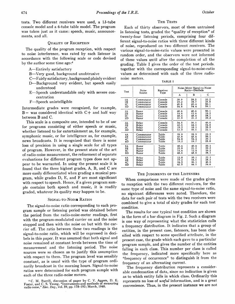
to reception with the two different receivers, for thesame type of noise and the same signal-to-noise ratio,no signicant differences were noted. Therefore, thedata for each pair of tests with the two receivers werecombined to give a total of sixty grades for each testcondition.The results for one typical test condition are shown

in the form of a bar diagram in Fig. 2. Such a diagramis one way of representing what the statistician callsa frequency distribution. It indicates that a group ofentities, in the present case, listeners, has been clas-sified with respect to some specified attribute, in thepresent case, the grade which each gave to a particularprogram sample, and gives the number of the entitiesfalling in each class. This number per class is calledthe frequency, indicated more specifically here as"frequency of occurrence" to distinguish it from thefrequency of an alternating current.The frequency distribution represents a consider-

able condensation of data, since no indication is givenas to which entity falls in which class. Ordinarily thisrepresents no loss of useful information, and is a greatconvenience. Thus, in the present instance we are not

October474

Burrill: Radio-Noise-Meter Performance

interested in the grades given by the individual listenier,but rather in the grades of the group as a whole.

Statisticians have found that nearly all frequencydistributions may be grouped into a few basic types.One of the simplest of these types is so often en-countered that it has been called the normal frequencydistribution. As we shall see, the data plotted in Fig.2 may be adjusted to yield a distribution of this type.The data represented by a frequency distribution maybe condensed further by calculating, in a manner de-pending on the type of distribution, certain parametersand using these to characterize or represent the distri-bution itself. Two kinds of such parameters, applicableto most types of frequency distribution, are those in-dicating "central tendency" and those indicating "dis-persion." In the language of our present example, wemay represent the data for each listening test by twoquantities which answer the questions, what is theconvergent trend of opinion, and how much do opin-ions differ?

It is easy to see that the opinions trend toward aboutD+ for the test to which Fig. 2 applies, but the statis-tician requires a more precise determination of thetrend or central tendency. From the number of statis-tical quantities useful in indicating the central tend-ency of such data we shall choose the simplest and theone most used-the arithmetic mean. For this purposewe must assign, somewhat arbitrarily, numericalvalues to the classes or grades. The data can then be

25

20 -

LuD

LL.

E E+ D D+CC+ BQUALITY

Fig. 2-The listeners' judgments for a typical test summarized inthe form of a bar diagram. Noise meters A and B, commutatornoise, signal-to-noise ratio= 28.7 decibels.

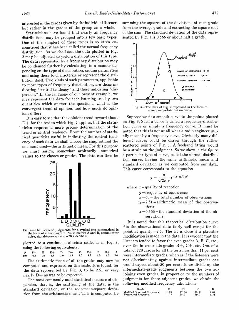
plotted to a continuous abscissa scale, as in Fig. 3,using the following equivalents:F F+ E E+ D D+ c C+ B B+ A0.0 0.5 1.0 1.5 2.0 2.5 3.0 3.5 4.0 4.5 5.0

The arithmetic mean of all the grades may now becomputed and expressed on this scale. It is found, forthe data represented by Fig. 3, to be 2.51 or verynearly D+ as was to be expected.The most commonly used statistical measure of dis-

persion, that is, the scattering of the data, is thestandard deviation, or the root-mean-square devia-tion from the arithmetic mean. This is computed by

summing the squares of the deviations of each gradefrom the average grade and extracting the square rootof the sum. The standard deviation of the data repre-sented by Fig. 3 is 0.566 or about half a grade.

50

40

30

NUMBER 0rOSSERVATIONS N-SO

°ARITHMETIC MEAN A- 2.51

0 20-

I.. STANDARD DEVIATION -p0j560

Z 10 0 OBSERVEDw0 / ADJUSTED

O _0 0 002OUAuTY or RECEPTION

Fig. 3-The data of Fig. 2 expressed in the form ofa frequency-distribution curve.

Suppose we fit a smooth curve to the points plottedon Fig. 3. Such a curve is called a frequency-distribu-tion curve or simply a frequency curve. It must benoted that this is not at all what a radio engineer usu-ally means by a frequency curve. Obviously many dif-ferent curves could be drawn through the ratherscattered points of Fig. 3. A freehand fitting wouldbe a strain on the judgment. So we show in the figurea particular type of curve, called the normal-distribu-tion curve, having the same arithmetic mean andstandard deviation as we computed from our data.This curve corresponds to the equation

n2y = _~ - 1E- (axa) 2l

-\/27r - o

where x = quality of receptiony =frequency of occurrencen = 60 = the total number of observationsxo = 2.51 =arithmetic mean of the observa-

tionsa= 0.566 = the standard deviation of the ob-

servationsIt is noted that this theoretical distribution curve

fits the observational data fairly well except for thepoint at quality = 2.5. The fit is close if a plausiblemodification is made in the data. It is evident that thelisteners tended to favor the even grades A, B, C, etc.,over the intermediate grades B+, C+, etc. Out of atotal of 720 grades for all the tests, less than 11 per centwere intermediate grades, whereas if the listeners werenot discriminating against intermediate grades onewould expect about 50 per cent. It we divide up theintermediate-grade judgments between the two ad-joining even grades, in proportion to the numbers ofjudgments for those adjacent grades, we obtain thefollowing modified frequency tabulation:

GradeModified Observed FrequencyTheoretical Frequency

E D c B1.09 27.66 30.21 1.041.23 28.2 29.0 1.33

4751942

476 Proceedings of the I.R.E. October

TABLE II

Quality of Reception Correlation

Noise Source Noise Meter Signal-to-Noise Standard Probable Error Regression Coeffiients Standard CoeficientRatio, Decibels Arithmetic Standardn f 6Mean Deviation Single Mean of 60 Error of of LinearMean Deviatio

Observation Observations a b Estimate Correlation

Direct-Current 19.4 1.742 0.511 0.347 0.0445Commutator A & B 28.7 2.508 0.566 0.385 0.0497 0.154 0.0826 0.612 0.882

Motor 45.6 4.025 0.602 0.409 0.052454.6 4.592 0.725 0.493 0.0631

13.6 0.842 0.566 0.382 0.0493Razor A & B 22.0 1.950 0.472 0.318 0.0411 -0.259 0.090 0.648 0.889

40.6 3.167 0.667 0.450 0.058148.6 4.233 0.735 0.496 0.0640

11.0 0.542 0.519 0.350 0.0452Relay A & B 18.6 1.683 0.533 0.360 0.0464 -0.3599 0.09625 0.590 0.903

35.3 2.892 0.611 0.412 0.053243.3 3.858 0.608 0.410 0.0529

- 25.0.Direct-Current C 332.2 Same as -0.328 0.0847 0.611 0.881Commutator 50.1

Motor 59.1

19.2Razor C 29.3 for Meters -0.615 0.0807 0.646 0.890

50.158.1

22.1Relay C 28.5 A and B -1.305 0.0935 0.508 0.929

46.6

54.6 08 00.6025l_ l96Averages 0.593 0.401 0.0516 - 0.08796 00.6025 0.896

The closeness of this fit of our data to the theoreti-cal normal-distribution curve permits and encouragesus to make certain assumptions from which usefulccnclusions can be drawn. Thus we postulate a statisti-cal population of all or a very large number of peoplelike those who participated as listeners in our tests,and we suppose our listeners to comprise a fair sampleselected at random from this population. We furtherassume that if the judgments of this entire populationregarding a given radio-program sample could betabulated they would turn out to be normally dis-tributed, that is, distributed in accordance with thenormal-distribution curve. It is also assumed that thearithmetic mean of the judgments of our samplegroup of listeners would coincide with the arithmeticmean of the judgments of the entire population.Now, under these assumptions, we can estimate

from our data the standard deviation of the entirepopulation, in accordance with the formula

_ n t-21/ n -1 . = / X 0.566 = 0.571.

From this value the probable error of a single judg-ment, and the probable error of the mean of a sampleof n judgments, in each case selected at random fromthe population, can be calculated. Thusprobable error of a

single observation= 0.6745s = 0.6745 / a

= 0.385.probable error of mean = 0.6745-= 0.6745of n observations In Vn - 1

= 0.0497.

The interpretation of these values is as follows:(1) The odds are even (probability 0.5) that the

judgment of a single listener chosen at random, re-

garding the particular program sample we have been

considering, would fall within ± 0.385 of a grade of thearithmetic mean obtained in our test.

(2) The odds are even that the arithmetic mean ofthe sixty judgments obtained from a second similargroup of listeners chosen at random would fall within+ 0.0497 of a grade of the arithmetic mean obtainedin our test.

In Table II are given the results of the grading foreach of the four noise levels and for each of the threetypes of noise. The arithmetic mean of the grades, theprobable error of this mean, and the probable errorof a single grade are tabulated. It is indicated thatvery satisfactory reliance can be placed on these data.

THE CORRELATION OF THE RADIO-NOISE-METER INDICATIONS

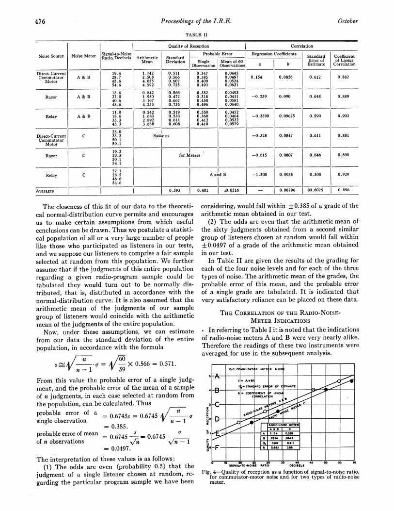
0 In referring to Table I it is noted that the indicationsof radio-noise meters A and B were very nearly alike.Therefore the readings of these two instruments wereaveraged for use in the subsequent analysis.

D-C CCMMUTATjR MOT R N015t

4 AR.. $TAN4ARD ERROR OF E]SMATE f U kCF-R N *

3

2

0IL

-C-

r%-L

-F-

- COE RELNT O UtN1RtELATl ON

I.i i -.-- p P., i _ __-.n 1RDI-NO

~4AI 0.

II I

laI.t2

ISE MEXTERi

.0647

WIS ~ ES EU ES EUI.<to Is 2 as 30 35 40 4 0 5 sSIGNAL-TO-NOISE RATIO DECIBELS

Fig. 4-Quality of reception as a function of signal-to-noise ratio,for commutator-motor noise and for two types of radio-noisemeter.

I ~~~~~~~~~~I

-,kf- _r' -"a'

A

Burrill: Radio-Noise-Meter Performance

Fig. 4 shows a plot of the quality of reception deter-mined by the arithmetic mean of the listeners' judg-ments, as a function of the signal-to-noise ratio indecibels indicated by the radio-noise meters. It repre-sents the tests with direct-current commutator-motornoise; similar plots for the other tests are shown inFigs. 5 and 6. It is evident that the observed pointsshown in Fig. 4 can be represented very well by twostraight lines, one for each type of radio-noise meter.Usually such straight lines would be drawn in simplyby inspection. However, in the present instance we

wish to determine a numerical measure of how wellthese lines represent the data, and so we must be care-

ful to obtain the "best" fit. This is obtained by themethod of least squares, by which the sum of thesquares of the deviations of the observational pointsfrom the line is made a minimum. The lines shownin the figure, which were obtained in this way, wouldbe called by statisticians linear regression lines; thecoefficients a and b in their algebraic expression, theregression equation y=a+bx would be called regres-sion coefficients.The usual measure of how well a regression line fits

the data is the "standard error of prediction." It isequal to the square root of the sum of the squares ofthe deviations of all the values of the dependent vari-able-'quality of reception" in the present case-as

predicted by the regression equation, from the cor-

responding observed values. This quantity (Te whichis made a minimum by the use of the method of leastsquares in determining the regression equation, is a

measure of the error to be expected in estimating a

value of y from the corresponding value of x and theregression equation.

Without any knowledge of x, the best estimate one

could make of a particular value of y would be thearithmetic mean of all the y values, and the error tobe expected would be measured by the square rootof the sum of the squares of the deviations of all of they values from this mean. This latter quantity is called

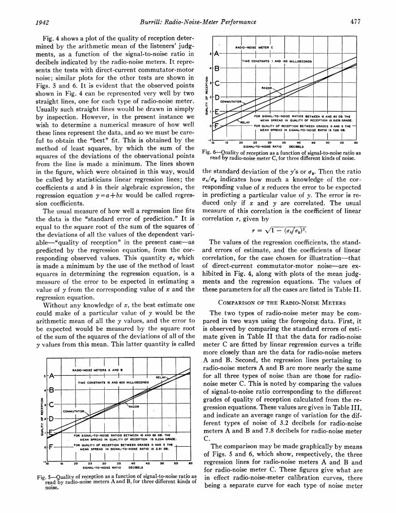
FORADIO-NOISEIETERBA ANDDi

5 A ~~~~~~~~RELYTIME CONSTANTS 10 AND 600MMILISECONDSS

1 FOR QUALITY OF RECEPTION BETWEEN GRADES 0 AND THE

I5 205 35 40 4S SO 55 60

SIGNAL-TO-NOISE RATIO DECIBELS

Fig. 5-Quality of reception as a function of signal-to-noise ratio asread by radio-noise meters A and B, for three different kinds ofnoise.

z

2

0

10 13 20 25 30 35 40 45 S0 55 60

SIGNAL-TO-NOISE RATIO DECIBELS

Fig. 6-Quality of reception as a function of signal-to-noise ratio as

read by radio-noise meter C, for three different kinds of noise.

the standard deviation of the y's or o-. Then the ratio

qe/O, indicates how much a knowledge of the cor-

responding value of x reduces the error to be expectedin predicting a particular value of y. The error is re-

duced only if x and y are correlated. The usualmeasure of this correlation is the coefficient of linearcorrelation r, given by

r = \/1- (oJ oUV).The values of the regression coefficients, the stand-

ard errors of estimate, and the coefficients of linearcorrelation, for the case chosen for illustration-thatof direct-current commutator-motor noise-are ex-

hibited in Fig. 4, along with plots of the mean judg-ments and the regression equations. The values ofthese parameters for all the cases are listed in Table II.

COMPARISON OF THE RADIO-NOISE METERSThe two types of radio-noise meter may be com-

pared in two ways using the foregoing data. First, itis observed by comparing the standard errors of esti-mate given in Table II that the data for radio-noisemeter C are fitted by linear regression curves a triflemore closely than are the data for radio-noise metersA and B. Second, the regression lines pertaining toradio-noise meters A and B are more nearly the same

for all three types of noise than are those for radio-noise meter C. This is noted by comparing the valuesof signal-to-noise ratio corresponding to the differentgrades of quality of reception calculated from the re-

gression equations. These values are given in Table III,and indicate an average range of variation for the dif-ferent types of noise of 3.2 decibels for radio-noisemeters A and B and 7.8 decibels for radio-noise meterC.

The comparison may be made graphically by means

of Figs. 5 and 6, which show, respectively, the threeregression -lines for radio-noise meters A and B andfor radio-noise meter C. These figures give what are

in effect radio-noise-meter calibration curves, therebeing a separate curve for each type of noise meter

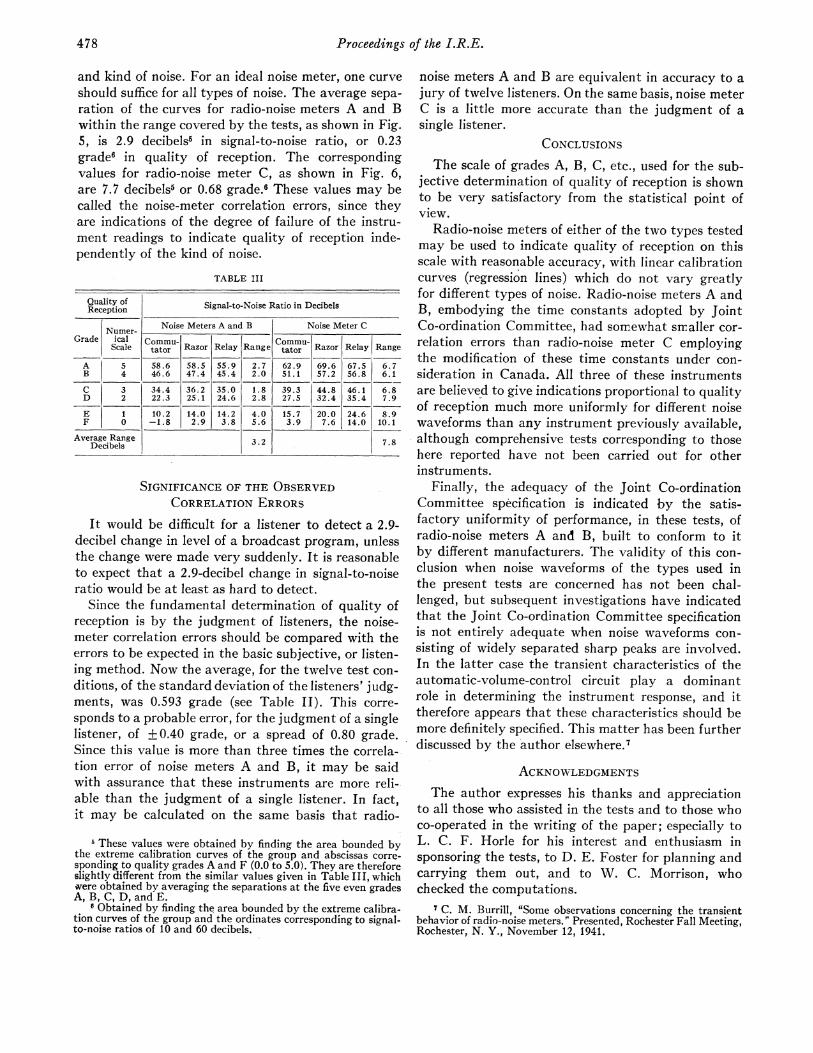
,ARADIO-NOISE METER C

TIME CONSTANTS AND 160 MILLISECONDS

2 CE MMUTATOR __

FOR SIGNAL-TO-NOISE RATIOS BETWEEN Ie AND O0 DB. THEMEAN SPREAD IN QUALITY OF RECEPTION 15 "78 GRADE.

o Ff FOR QUALITY OF RECEPTION BETWEEN GRADES 0 AND 5 THEMEAN SPREAD IN SIGNAL-TO-NOISE RATIO IS 786 DB.

4771942

Proceedings of the I.R.E.

and kind of noise. For an ideal noise meter, one curveshould suffice for all types of noise. The average sepa-ration of the curves for radio-noise meters A and Bwithin the range covered by the tests, as shown in Fig.5, is 2.9 decibels5 in signal-to-noise ratio, or 0.23grade6 in quality of reception. The correspondingvalues for radio-noise meter C, as shown in Fig. 6,are 7.7 decibels5 or 0.68 grade.5 These values may becalled the noise-meter correlation errors, since theyare indications of the degree of failure of the instru-ment readings to indicate quality of reception inde-pendently of the kind of noise.

TABLE III

Quality of Signal-to-Noise Ratio in DecibelsReception

Numer- Noise Meters A and B Noise Meter CGrade ical Commu- Commu-Scale tator Razor Relay Range tator Razor Relay Range

A 5 58.6 58.5 55.9 2.7 62.9 69.6 67.5 6.7B 4 46.6 47.4 45.4 2.0 51.1 57.2 56.8 6.1

C 3 34.4 36.2 35.0 1.8 39.3 44.8 46.1 6.8D 2 22.3 25.1 24.6 2.8 27.5 32.4 35.4 7.9

E 1 10.2 14.0 14.2 4.0 15.7 20.0 24.6 8.9F 0 -1.8 2.9 3.8 5.6 3.9 7.6 14.0 10.1

Average Range 3.2 7.8Decibels

.

SIGNIFICANCE OF THE OBSERVEDCORRELATION ERRORS

It would be difficult for a listener to detect a 2.9-decibel change in level of a broadcast program, unlessthe change were made very suddenly. It is reasonableto expect that a 2.9-decibel change in signal-to-noiseratio would be at least as hard to detect.

Since the fundamental determination of quality ofreception is by the judgment of listeners, the noise-meter correlation errors should be compared with theerrors to be expected in the basic subjective, or listen-ing method. Now the average, for the twelve test con-

ditions, of the standard deviation of the listeners' judg-ments, was 0.593 grade (see Table II). This corre-

sponds to a probable error, for the judgment of a singlelistener, of +0.40 grade, or a spread of 0.80 grade.Since this value is more than three times the correla-tion error of noise meters A and B, it may be saidwith assurance that these instruments are more reli-able than the judgment of a single listener. In fact,it may be calculated on the same basis that radio-

These values were obtained by finding the area bounded bythe extreme calibration curves of the group and abscissas corre-sponding to quality grades A and F (0.0 to 5.0). They are thereforeslightly different from the similar values given in Table III, whichwvere obtained by averaging the separations at the five even gradesA, B, C, D, and E.

'Obtained by finding the area bounded by the extreme calibra-tion curves of the group and the ordinates corresponding to signal-to-noise ratios of 10 and 60 decibels.

noise meters A and B are equivalent in accuracy to ajury of twelve listeners. On the same basis, noise meterC is a little more accurate than the judgment of asingle listener.

CONCLUSIONSThe scale of grades A, B, C, etc., used for the sub-

jective determination of quality of reception is shownto be very satisfactory from the statistical point ofview.

Radio-noise meters of either of the two types testedmay be used to indicate quality of reception on thisscale with reasonable accuracy, with linear calibrationcurves (regression lines) which do not vary greatlyfor different types of noise. Radio-noise meters A andB, embodying the time constants adopted by JointCo-ordination Committee, had somewhat smraller cor-relation errors than radio-noise meter C employingthe modification of these time constants under con-sideration in Canada. All three of these instrumentsare believed to give indications proportional to qualityof reception much more uniformly for different noisewaveforms than any instrument previously available,although comprehensive tests corresponding to thosehere reported have not been carried out for otherinstruments.

Finally, the adequacy of the Joint Co-ordinationCommittee specification is indicated by the satis-factory uniformity of performance, in these tests, ofradio-noise meters A and B, built to conform to itby different manufacturers. The validity of this con-clusion when noise waveforms of the types used inthe present tests are concerned has not been chal-lenged, but subsequent investigations have indicatedthat the Joint Co-ordination Committee specificationis not entirely adequate when noise waveforms con-sisting of widely separated sharp peaks are involved.In the latter case the transient characteristics of theautomatic-volume-control circuit play a dominantrole in determining the instrument response, and ittherefore appears that these characteristics should bemore definitely specified. This matter has been furtherdiscussed by the author elsewhere.7

ACKNOWLEDGMENTSThe author expresses his thanks and appreciation

to all those who assisted in the tests and to those whoco-operated in the writing of the paper; especially toL. C. F. Horle for his interest and enthusiasm insponsoring the tests, to D. E. Foster for planning andcarrying them out, and to W. C. Morrison, whochecked the computations.

7 C. M. Burrill, "Some observations concerning the transientbehavior of radio-noise meters.' Presented, Rochester Fall Meeting,Rochester, N. Y., November 12, 1941.

1478