an environment-aware mobility model for wireless ad hoc network

Computer Networks 54 (2010) 1470–1489

Contents lists available at ScienceDirect

Computer Networks

journal homepage: www.elsevier .com/locate /comnet

An environment-aware mobility model for wireless ad hoc network

Sabbir Ahmed *, Gour C. Karmakar, Joarder KamruzzamanGippsland School of Information Technology, Monash University, Churchill, VIC 3842, Australia

a r t i c l e i n f o

Article history:Received 23 March 2009Received in revised form 26 November 2009Accepted 10 December 2009Available online 16 December 2009Responsible Editor: L. Jiang Xie

Keywords:Ad hoc networkMobility modelEnvironment-aware

1389-1286/$ - see front matter � 2009 Elsevier B.Vdoi:10.1016/j.comnet.2009.12.005

* Corresponding author. Tel.: +61 51226143.E-mail addresses: [email protected] (S. Ahm

monash.edu.au (G.C. Karmakar), joarder@infotecKamruzzaman).

a b s t r a c t

Simulation is a cost effective, fast and flexible alternative to test-beds or practical deploy-ment for evaluating the characteristics and potential of mobile ad hoc networks. Sinceenvironmental context and mobility have a great impact on the accuracy and efficacy ofperformance measurement, it is of paramount importance how closely the mobility of anode resembles its movement pattern in a real-world scenario. The existing mobility mod-els mostly assume either free space for deployment and random node movement or themovement pattern does not emulate real-world situation properly in the presence ofobstacles because of their generation of restricted paths. This demands for the develop-ment of a node movement pattern with accurately representing any obstacle and existingpath in a complex and realistic deployment scenario. In this paper, we propose a generalmobility model capable of creating a more realistic node movement pattern by exploitingthe concept of flexible positioning of anchors. Since the model places anchors dependingupon the context of the environment through which nodes are guided to move towardsthe destination, it is capable of representing any terrain realistically. Furthermore, obsta-cles of arbitrary shapes with or without doorways and any existing pathways in full or partof the terrain can be incorporated which makes the simulation environment more realistic.A detailed computational complexity has been analyzed and the characteristics of the pro-posed mobility model in the presence of obstacles in a university campus map with andwithout signal attenuation are presented which illustrates its significant impact on perfor-mance evaluation of wireless ad hoc networks.

� 2009 Elsevier B.V. All rights reserved.

1. Introduction

Mobile ad hoc networks (MANET) enable wireless com-munication between mobile devices without the existenceof a predefined infrastructure. Each of the devices works asa sender, receiver as well as router. Such networks have awide range of applications including data transmission indisaster areas, battlefield and inter vehicular communica-tion because of its ability of ad hoc deployment as wellas lower cost and reduced complexity than establishingand maintaining an infrastructure.

. All rights reserved.

ed), [email protected] (J.

Over the last decade, huge research efforts have beendedicated to the theoretical development and analysis ofMANET in relation to capacity estimation, routing, scalabil-ity, location service, mobility modeling, performance evalu-ation and others. Such theoretical study can only be verifiedthrough test-beds, real-world deployment or appropriatesimulation tools that emulate practical scenarios. Simula-tion environment is very attractive for evaluating perfor-mance of MANET through various metrics, since it reducesthe huge cost and time for real world study through test-beds or practical deployment. It helps to generate a widevariety of repeatable scenarios, which may not be possibleto test in real-world deployment for evaluation purpose.This repeatable scenario generation aids to analyze differentperspective of the network performance, through variousperformance metrics, and readjustment of protocols under

http://dx.doi.org/10.1016/j.comnet.2009.12.005

mailto:[email protected]




http://www.sciencedirect.com/science/journal/13891286

http://www.elsevier.com/locate/comnet

S. Ahmed et al. / Computer Networks 54 (2010) 1470–1489 1471

consideration is possible [1]. Due to the capability of rapiddevelopment of wide range of scenarios within short timeand scope for refinements, protocol designers use simula-tion tools for investigating the performance of protocols.But, for accurate evaluation of MANET models, simulationenvironment must be based on realistic assumptions, with-out which simulation becomes ineffectual.

One of the key factors for a simulation environment toreflect and assess real-world scenario accurately is to mod-el node mobility in MANET as realistically as possible. Afterdeployment of nodes, the mobility model used in simula-tion is responsible for directing the nodes when and whereto move. A variety of mobility models that has been pro-posed in literature for studying mobile network are de-scribed in Section 2. Among them Random Waypointmodel, Random Walk model and Random Direction modelare widely used where nodes are assumed to be deployedin a rectangular sized unobstructed simulation area. Nodescan move any where in the given simulation playgroundaccording to the specification of the respective mobilitymodel.

In most of the existing mobility models nodes move in arandom fashion in free space, but real world is rather com-plex and vastly diverse that make the existing modelsinappropriate of representing the real world context prop-erly. The essential constituents of a natural environmentare pathways and obstacles. We often find many obstaclessuch as buildings, lakes, hills, playgrounds, vegetation thatrestrict our movement in different ways. Here, by the word‘‘obstacle”, we refer to both accessible (e.g., buildings) andinaccessible (e.g., lakes, hills, restricted area) objects ob-served in the environment. Irrespective of the position ofpathways, obstacles and their entry points in a real worldsetup, existing obstacle based mobility model [1] producesa fixed number of restricted paths and entry points to eachside of an obstacle and uses shortest path for node move-ment. However, there are some obstacles, e.g., buildings,where people can move inside and others where they arenot expected to enter e.g., hills. People also do not movein a random fashion rather a region of interest basis; usu-ally they have specific regions/destinations in mind to go.There may be defined pathways or no pathways at all forgoing to a specific region. In many cases people do notuse shortest paths to reach the destination. To address thisand hence a major unresolved problem, ‘‘there can be nosingle model that is the best for all terrains” [1], it is essen-tial to develop a mobility model where node movement isguided considering the elements of a deployment context,such as obstacles and existing pathways and a frameworkwhich could accurately represent their natural structures.In this paper, this is accomplished by exploiting the flexiblepositioning of anchors in simulated deployment area andproposing a novel mobility model called anchor-basedmobility model (AMM).

Our proposed mobility model incorporates all of theabove mentioned real world features. Anchors are assumedto be square shaped geographic positions and can be lo-cated anywhere in the deployment area depending onthe context such as predefined path, obstacles and theirentry points, if exist. Therefore, their positions in a way de-fine the mobility framework in the deployment area. For

example, anchors can be defined around each convex cor-ner of an obstacle and entry points. Thus anchors will con-tribute to generating a graph that will guide the nodemovement in an appropriate way. A node can reach anyposition in the simulation area by selecting a suitable an-chor as the next step. The size of an anchor defines thefreedom and flexibility of the node movement. Sinceaccording to this model a node selects a random point inthe next anchor to be visited, it can produce a more flexiblenode movement scenario which is able to capture a widevariety of movement pattern. The model also reduces thesurrounding effect [2]. A basic version of this model in briefwas presented in [3]. The model was since then further ex-tended with additional features including incorporatingsignal fading. The model with further extensive simulationresults and analyses are presented in this paper. The maincontributions of this work are as follows:

� Proposed a new mobility model that generates nodemovement patterns more realistically than the existingmobility models, and thereby, more suitable to simulateMANET in real-world deployment because of the follow-ing reasons:

[–] Facility to introduce any arbitrary shaped obsta-cles. Obstacles within an obstacle in a nested fashioncan also be supported. Moreover, internal floor-planof a building can be adopted as well.[–] Placement of doorways at any position in eachside of an obstacle (e.g., building) so that nodescan move inside the obstacle through the doors only.[–] Feature to adopt existing pathways in any or fullportion of the simulation area.[–] Computing node movement based on thedynamically generated anchors.[–] Allows visualizing the node movement and gen-erated mobility traces.

� Analyzed computational complexity of the model indetail and assessed impact of the model on the measure-ment of different network performance evaluation met-rics with and without signal attenuation due to thepresence of obstacles.

� Developed a GUI based program ‘‘MobiGen” thatincludes all the above features and generates nodemovement scenario files which can easily be integratedwith any network simulator e.g., ns2 [4].

To evaluate our mobility model, we used a real worldenvironment map of the Clayton campus, Monash Univer-sity, Australia with infrastructures in exact positions in thesimulation setup. Greedy Perimeter Stateless Routing(GPSR) [5] which uses geographic location of destinationto forward data is used as the routing protocol because ofits scalability to large networks and low packet overhead.Our mobility model is compared with the widely usedVoronoi graph based obstacle model [1] as it is capable ofgenerating scenarios in the presence of obstacles. Simula-tion results show that our proposed model has significantimpact on the performance of geographic routing protocolGPSR; most importantly, it simulates the true movementpattern of a node under a real-world scenario more closelythan other mobility models.

1472 S. Ahmed et al. / Computer Networks 54 (2010) 1470–1489

2. Related works

A variety of mobility models have been introduced inthe literature, detail survey of which can be found in [6–10]. They can be mainly classified into two main streams:

(1) Trace-based models(2) Synthetic models

Traces are mobility patterns generated from real-worldsystem, mainly by analyzing stored information in existingnetwork system with a large number of participants over along observation period. Patterson et al. [11] tried to iden-tify common destinations in a user’s daily life with GPSdata. Another prominent work involves Weighted WayPoint model [12], where 268 students were asked to main-tain diary with their daily movement for a period of onemonth. These movements were mainly focused to class-rooms, library, cafeteria and off-campus. With this surveydata the authors tried to identify the distribution of visitingthose locations and pause time, and developed a Markovbased model. A more recent work is done by Kim et al.[13] with the Wi-Fi network traces collected at DartmouthCollege comprising approximately 560 access points witharound 10,000 users over several years. While users move,they register with the nearest access points and, with thisstored information, the authors extracted a syntheticmobility model by identifying hot spot regions with distri-bution of pause time. But as stated in [13], the extractedmobility model describes user movement from one hotspot to another but does not validate the real path takenbetween hotspots.

However, as stated in [6], it is hard to simulate a newnetwork environment if traces have not yet been createdusing an existing setup established for a quite long time.Moreover, since MANETs have not been deployed on awide scale, obtaining real mobility traces becomes a majorchallenge [7]. For this reason Synthetic models are devel-oped. Here, researchers proposed different types of mobil-ity models where mobile users and their movement pathswere created probabilistically and attempted to capturevarious characteristics of realistic mobility. A detailed clas-sification of models is shown in Fig. 1.

A variety of synthetic mobility models have been pro-posed in literature for generating node movement pattern.These models can be further categorized into two groups

Mobility Models

Trace-based Models Synthetic Models

Free SpaceModels

Geographic RestrictedModels

Fig. 1. Categories of mobility models.

based on their consideration of environmental attributes:(a) Free space model and (b) Geographic restricted models.

Random Waypoint model is one of the mostly usedmodels where a node randomly selects one location inthe simulation space as destination. It then travels towardsthe destination with a constant velocity chosen uniformlyand randomly within the range of ½0;vmax�, where vmax rep-resents the maximum allowable velocity and pauses forTpause, termed as pause time. The whole process continuesto repeat until the simulation ends. The spatial node distri-bution of Random Waypoint model is transformed fromuniform distribution to non-uniform distribution afterthe simulation starts [14]. As the simulation time elapses,the imbalance in spatial node distribution becomesprominent.

Random Direction model [15] was introduced to over-come the density waves in the average number of neighborsand the non-uniform spatial distribution, produced by theRandom Waypoint model. In Random Direction model, anode chooses a random direction and speed uniformly dis-tributed between ½0;2p� and ½0;vmax�, respectively. Whilemoving towards that direction, when a node reaches theboundary, it pauses for Tpause, then again randomly selectsanother direction and speed, and continues this processuntil the simulation ends. Since nodes are allowed to movetowards the boundary of simulation area, nodes at theboundary are expected to have lower density functioncompared to the ones in the middle. Moreover, a portionof boundary nodes transmission area that extends beyondthe boundary becomes useless, resulting in non-uniformnumber of neighbors and link duration that consequentlyaffect effective connectivity measurement. This phenom-ena is termed as boundary effect.

A slight modification to this model has also been pro-posed by the same authors where nodes continue to chooserandom directions but they are no longer forced to travel tothe simulation boundary. Before stopping to change direc-tion, a node chooses a random direction and selects a desti-nation anywhere along that direction of travel. The nodethen pauses at this destination before choosing a new direc-tion. Boundless Simulation Area model was introduced toalleviate the boundary effect observed in Random Directionmodel. In this model [16], nodes that reach one side of thesimulation area continue traveling and reappear on theopposite side of the simulation area. This technique createsa torus-shaped simulation area allowing the nodes to travelunobstructed. Though Boundless Simulation Area modeleffectively reduces the boundary effect, node movementseems unrealistic because of their reappearing at the oppo-site side of the simulation area.

In Random Walk model the nodes change their speedand direction at each time interval. For every interval, eachnode randomly and uniformly chooses a new direction hðtÞ,within the range ½0;2p�, and a new speed vðtÞ, which fol-lows the uniform distribution or the Gaussian distributionwithin ½vmin;vmax�, and then moves in the direction at thatspeed for either a specified number of steps or a time per-iod. At the end of the period, the nodes repeat this process.Leng et al. [17] analyzed host mobility characteristics in adhoc network in terms of link available time and number oflink change in random walk model.


The Gauss–Markov Mobility model was designed tointroduce temporal dependency in mobility model. Initiallyeach node is assigned speed and direction. Afterward the va-lue of speed and direction at the nth instance is calculated onthe basis of the value of speed and direction at the ðn� 1Þthinstance, and a random variable a tunes the randomness.

Group mobility models have been introduced to get apicture of the situations where the nodes or a subset ofnodes move as a group and thus considers spatial depen-dency. Among the group mobility models found in the lit-erature, Reference Point Group Mobility model [18] ismostly used. In this scheme, the random motion of a groupof mobile nodes is defined as well as the random motion ofeach individual node within the group. A logical center ofeach group is developed and the movements are basedon the path traveled by a logical center for the group. Indi-vidual nodes randomly move around their own predefinedreference points, maintaining a more or less relative dis-tance with the group center. A variation of Reference PointGroup Mobility model is Nomadic Community Mobilitymodel [6]. In this model a group maintains a referencepoint and the nodes within the group can move aroundthe reference point with a given degree of flexibility. Eachnode uses any of the random mobility models and its flex-ibility of movement from the reference point is defined bythe parameters of the random mobility model it is using.This type of mobility model can be observed when a groupof children visits a museum where they follow a guide androam around with somewhat degree of freedom. Aftersome time interval, the reference point moves and all thenodes in that group also move along with it.

Some other varieties of group mobility models are Pur-sue Mobility model [6] that attempts to represent a groupof mobile nodes tracking a particular target node, just likea group of police chasing a criminal, and Column Mobilitymodel [19] which is useful for scanning or searching pur-poses where nodes are allowed to move around a givencolumn (line).

As described above, each of these mobility models as-sumes open and unobstructed areas where the nodes canmove freely, but in real-world situation the existence ofthis type of unobstructed scenario is rare, and thereby,they fail to generate the true node movements for a realworld environment. For this reason researchers attemptedto introduce environmental attributes in mobility models,which are classified as Geographic restricted mobility model.

A few mobility models [20] that take geographic restric-tions into account are Pathway Mobility model and Obsta-cle Mobility model. Pathway Mobility model uses apredefined map in the simulation field. Some researchers[21] utilized random graph to model the map of a city.The graph is generated either randomly or based on themap of a real city, where the vertices represent the build-ings and the edges model the streets and freeways linkingthose buildings. Nodes are allowed to move only on thepredefined edges. Variations of this mobility model areFreeway and Manhattan Mobility model, where the mobil-ity model mainly focuses on car movement on the free-ways connecting different cities and streets in horizontalor vertical directions, respectively, and are more suitablefor cellular network rather than MANET.

Another variation of Pathway Mobility model is AgendaDriven Mobility model [22,23] that also utilizes streets andpathways. In this model a node selects its destinationbased on agenda – a social interaction policy that describesits movement by specifying when and where to move. Forinstance, in a typical weekday, a student could leave homein the morning, visit the university, attend classes and inthe evening come back home. While moving towards adestination, nodes use existing streets and pathways. Orbi-tal Mobility model [24] also utilizes social interactionwhile making movement decision but uses free space assimulation environment.

In Obstacle Mobility model rudimentary obstacles inthe form of buildings of regular shape are distributed ran-domly or based on a map throughout the simulation area.While moving in the simulation area whenever a nodefaces an obstacle on the way, it changes its direction andstarts moving again. Johansson et al. [25] developed threemobility scenarios to depict the movement of mobile usersin real life which includes Conference, Event Coverage andDisaster Relief scenarios. Jardosh et al. [1] also investigatedthe impact of obstacles on mobility modeling in detail. Intheir simulation field, a number of obstacles were placedto model the buildings within a campus environment. Theyused a Voronoi graph to compute the movement path forthe nodes. Nodes are only allowed to move on the edgesof the Voronoi cells. After choosing a new destination onthe pathway graph randomly, a node moves towards itby following the shortest path through the generated path-way graph.

Though the Geographic restricted mobility models givea flavor of realistic movement of mobile nodes suitable forMANETs, some essential elements of real world mobilityare still lacking. The Voronoi graph based model uses onlybuildings of regular shapes as obstacles and restricts thenode movement only on the edges of the Voronoi cells,thus lacking the randomness of movement in the area,since people are not always expected to move on prede-fined paths. As a result, this model is incapable of generat-ing a wide range of node movement variations. Also theposition of doorways in buildings derived from Voronoigraph may stray from the actual position of the doors, allsides of a building may not contain doors, and conse-quently, the model fails to capture an actual environment.These reasons motivated us to develop a mobility modelcapable of capturing node mobility more realisticallybelonging to the group Geographic restricted model.

3. Need for a realistic mobility model

As alluded in Section 1, ad hoc network is attractive forcommunication in battlefields, disaster areas and intervehicular communication where it embraces a huge num-ber of different deployment contexts. In disaster areas afterearthquake, flood, fire or war there might be many build-ings, streets and roads destroyed. Established road infra-structure may be totally or partially damaged. Rescueoperators may need to save people stuck under demol-ished or semi-demolished buildings. In absence or demoli-tion of existing infrastructure, peoples movement cannot

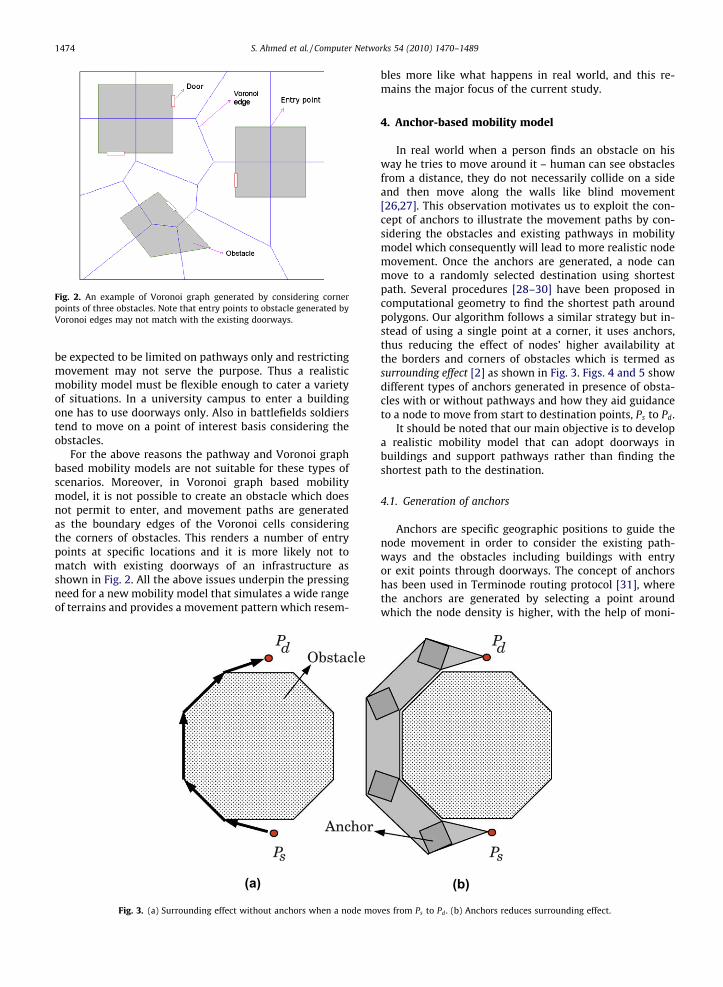
Fig. 2. An example of Voronoi graph generated by considering cornerpoints of three obstacles. Note that entry points to obstacle generated byVoronoi edges may not match with the existing doorways.


be expected to be limited on pathways only and restrictingmovement may not serve the purpose. Thus a realisticmobility model must be flexible enough to cater a varietyof situations. In a university campus to enter a buildingone has to use doorways only. Also in battlefields soldierstend to move on a point of interest basis considering theobstacles.

For the above reasons the pathway and Voronoi graphbased mobility models are not suitable for these types ofscenarios. Moreover, in Voronoi graph based mobilitymodel, it is not possible to create an obstacle which doesnot permit to enter, and movement paths are generatedas the boundary edges of the Voronoi cells consideringthe corners of obstacles. This renders a number of entrypoints at specific locations and it is more likely not tomatch with existing doorways of an infrastructure asshown in Fig. 2. All the above issues underpin the pressingneed for a new mobility model that simulates a wide rangeof terrains and provides a movement pattern which resem-

(a)

Fig. 3. (a) Surrounding effect without anchors when a node mo

bles more like what happens in real world, and this re-mains the major focus of the current study.

4. Anchor-based mobility model

In real world when a person finds an obstacle on hisway he tries to move around it – human can see obstaclesfrom a distance, they do not necessarily collide on a sideand then move along the walls like blind movement[26,27]. This observation motivates us to exploit the con-cept of anchors to illustrate the movement paths by con-sidering the obstacles and existing pathways in mobilitymodel which consequently will lead to more realistic nodemovement. Once the anchors are generated, a node canmove to a randomly selected destination using shortestpath. Several procedures [28–30] have been proposed incomputational geometry to find the shortest path aroundpolygons. Our algorithm follows a similar strategy but in-stead of using a single point at a corner, it uses anchors,thus reducing the effect of nodes’ higher availability atthe borders and corners of obstacles which is termed assurrounding effect [2] as shown in Fig. 3. Figs. 4 and 5 showdifferent types of anchors generated in presence of obsta-cles with or without pathways and how they aid guidanceto a node to move from start to destination points, Ps to Pd.

It should be noted that our main objective is to developa realistic mobility model that can adopt doorways inbuildings and support pathways rather than finding theshortest path to the destination.

4.1. Generation of anchors

Anchors are specific geographic positions to guide thenode movement in order to consider the existing path-ways and the obstacles including buildings with entryor exit points through doorways. The concept of anchorshas been used in Terminode routing protocol [31], wherethe anchors are generated by selecting a point aroundwhich the node density is higher, with the help of moni-

(b)

ves from Ps to Pd . (b) Anchors reduces surrounding effect.

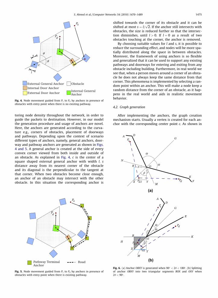
Fig. 4. Node movement guided from Ps to Pd by anchors in presence ofobstacles with entry point when there is no existing pathway.


toring node density throughout the network, in order toguide the packets to destination. However, in our modelthe generation procedure and usage of anchors are novel.Here, the anchors are generated according to the curva-ture e.g., corners of obstacles, placement of doorwaysand pathways. Depending upon the context of scenariodifferent types of anchors, namely, general anchors, door-way and pathway anchors are generated as shown in Figs.4 and 5. A general anchor is created at the side of everyconvex corner viewed from both inside and outside ofan obstacle. As explained in Fig. 4, c is the center of asquare shaped external general anchor with width l; sdistance away from its nearest corner of the obstacleand its diagonal is the perpendicular to the tangent atthat corner. When two obstacles become close enough,an anchor of an obstacle may intersect with the otherobstacle. In this situation the corresponding anchor is

Fig. 5. Node movement guided from Ps to Pd by anchors in presence ofobstacles with entry point when there is existing pathway.

shifted towards the corner of its obstacle and it can beshifted at most s ¼ l=

ffiffiffi2p

. If the anchor still intersects withobstacles, the size is reduced further so that the intersec-tion diminishes, until l > 0. If l ¼ 0 as a result of twoobstacles touching at the corner, the anchor is removed.

By choosing suitable values for l and s, it is possible toreduce the surrounding effect, and nodes will be more spa-tially distributed along the space in between obstacles.Moreover, the framework of using anchors is so flexibleand generalized that it can be used to support any existingpathways and doorways for entering and exiting from anyobstacle including building. Furthermore, in real world wesee that, when a person moves around a corner of an obsta-cle he does not always keep the same distance from thatcorner. This phenomena is implemented by selecting a ran-dom point within an anchor. This will make a node keep arandom distance from the corner of an obstacle, as it hap-pens in the real world and aids in realistic movementbehavior.

4.2. Graph generation

After implementing the anchors, the graph creationmechanism starts. Usually a vertex is created for each an-chor with the corresponding center point c. As shown in

(a)

(b)

Fig. 6. (a) Anchor OBXY is generated when 90� < 2h < 180� . (b) Splittingof anchor OBXY into two triangular segments BOX and OXY when2h < 90� .

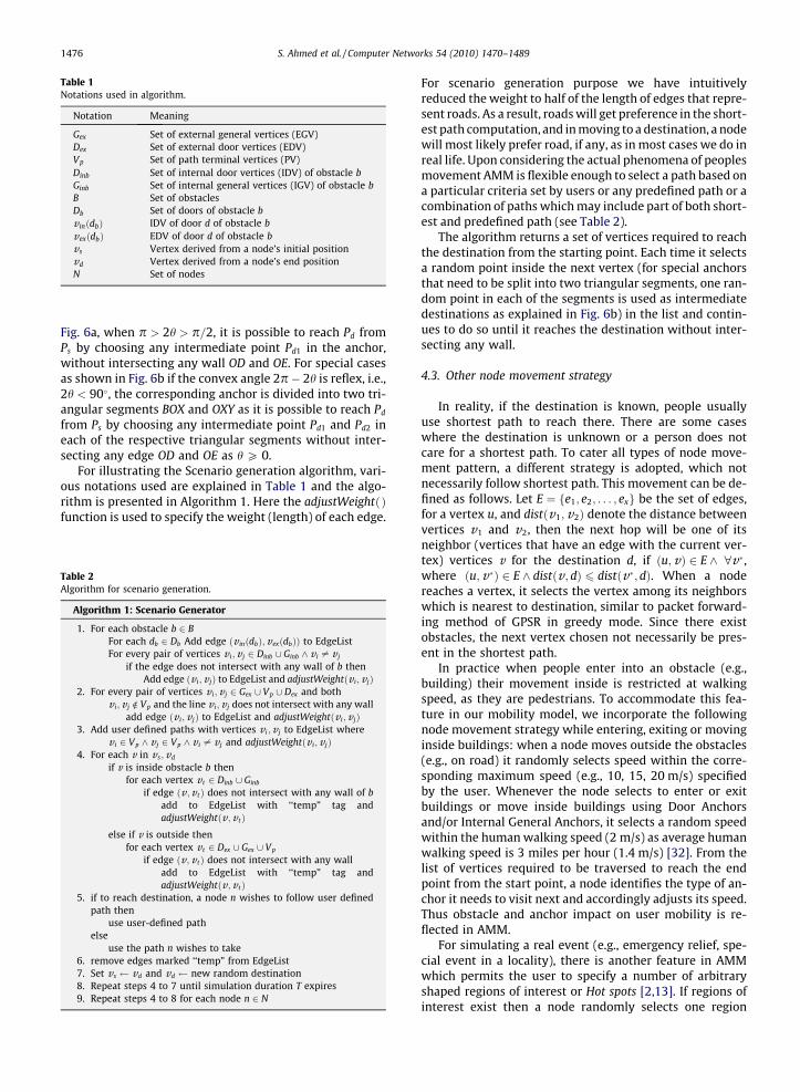
Table 1Notations used in algorithm.

Notation Meaning

Gex Set of external general vertices (EGV)Dex Set of external door vertices (EDV)Vp Set of path terminal vertices (PV)Dinb Set of internal door vertices (IDV) of obstacle bGinb Set of internal general vertices (IGV) of obstacle bB Set of obstaclesDb Set of doors of obstacle bv inðdbÞ IDV of door d of obstacle bvexðdbÞ EDV of door d of obstacle bvs Vertex derived from a node’s initial positionvd Vertex derived from a node’s end positionN Set of nodes


Fig. 6a, when p > 2h > p=2, it is possible to reach Pd fromPs by choosing any intermediate point Pd1 in the anchor,without intersecting any wall OD and OE. For special casesas shown in Fig. 6b if the convex angle 2p� 2h is reflex, i.e.,2h < 90�, the corresponding anchor is divided into two tri-angular segments BOX and OXY as it is possible to reach Pd

from Ps by choosing any intermediate point Pd1 and Pd2 ineach of the respective triangular segments without inter-secting any edge OD and OE as h P 0.

For illustrating the Scenario generation algorithm, vari-ous notations used are explained in Table 1 and the algo-rithm is presented in Algorithm 1. Here the adjustWeightðÞfunction is used to specify the weight (length) of each edge.

Table 2Algorithm for scenario generation.

Algorithm 1: Scenario Generator

1. For each obstacle b 2 BFor each db 2 Db Add edge ðv inðdbÞ;vexðdbÞÞ to EdgeListFor every pair of vertices v i;v j 2 Dinb [ Ginb ^ v i – v j

if the edge does not intersect with any wall of b thenAdd edge ðv i; v jÞ to EdgeList and adjustWeightðv i; v jÞ

2. For every pair of vertices v i; v j 2 Gex [ Vp [ Dex and bothv i; v j R Vp and the line v i; v j does not intersect with any wall

add edge ðv i; v jÞ to EdgeList and adjustWeightðv i; v jÞ3. Add user defined paths with vertices v i; v j to EdgeList where

v i 2 Vp ^ v j 2 Vp ^ v i – v j and adjustWeightðv i; v jÞ4. For each v in v s;vd

if v is inside obstacle b thenfor each vertex v t 2 Dinb [ Ginb

if edge ðv ;v tÞ does not intersect with any wall of badd to EdgeList with ‘‘temp” tag andadjustWeightðv ; v tÞ

else if v is outside thenfor each vertex v t 2 Dex [ Gex [ Vp

if edge ðv ; v tÞ does not intersect with any walladd to EdgeList with ‘‘temp” tag andadjustWeightðv ; v tÞ

5. if to reach destination, a node n wishes to follow user definedpath then

use user-defined pathelse

use the path n wishes to take6. remove edges marked ‘‘temp” from EdgeList7. Set v s vd and vd new random destination8. Repeat steps 4 to 7 until simulation duration T expires9. Repeat steps 4 to 8 for each node n 2 N

For scenario generation purpose we have intuitivelyreduced the weight to half of the length of edges that repre-sent roads. As a result, roads will get preference in the short-est path computation, and in moving to a destination, a nodewill most likely prefer road, if any, as in most cases we do inreal life. Upon considering the actual phenomena of peoplesmovement AMM is flexible enough to select a path based ona particular criteria set by users or any predefined path or acombination of paths which may include part of both short-est and predefined path (see Table 2).

The algorithm returns a set of vertices required to reachthe destination from the starting point. Each time it selectsa random point inside the next vertex (for special anchorsthat need to be split into two triangular segments, one ran-dom point in each of the segments is used as intermediatedestinations as explained in Fig. 6b) in the list and contin-ues to do so until it reaches the destination without inter-secting any wall.

4.3. Other node movement strategy

In reality, if the destination is known, people usuallyuse shortest path to reach there. There are some caseswhere the destination is unknown or a person does notcare for a shortest path. To cater all types of node move-ment pattern, a different strategy is adopted, which notnecessarily follow shortest path. This movement can be de-fined as follows. Let E ¼ fe1; e2; . . . ; exg be the set of edges,for a vertex u, and distðv1;v2Þ denote the distance betweenvertices v1 and v2, then the next hop will be one of itsneighbor (vertices that have an edge with the current ver-tex) vertices v for the destination d, if ðu;vÞ 2 E ^ 8v�,where ðu;v�Þ 2 E ^ distðv; dÞ 6 distðv�; dÞ. When a nodereaches a vertex, it selects the vertex among its neighborswhich is nearest to destination, similar to packet forward-ing method of GPSR in greedy mode. Since there existobstacles, the next vertex chosen not necessarily be pres-ent in the shortest path.

In practice when people enter into an obstacle (e.g.,building) their movement inside is restricted at walkingspeed, as they are pedestrians. To accommodate this fea-ture in our mobility model, we incorporate the followingnode movement strategy while entering, exiting or movinginside buildings: when a node moves outside the obstacles(e.g., on road) it randomly selects speed within the corre-sponding maximum speed (e.g., 10, 15, 20 m/s) specifiedby the user. Whenever the node selects to enter or exitbuildings or move inside buildings using Door Anchorsand/or Internal General Anchors, it selects a random speedwithin the human walking speed (2 m/s) as average humanwalking speed is 3 miles per hour (1.4 m/s) [32]. From thelist of vertices required to be traversed to reach the endpoint from the start point, a node identifies the type of an-chor it needs to visit next and accordingly adjusts its speed.Thus obstacle and anchor impact on user mobility is re-flected in AMM.

For simulating a real event (e.g., emergency relief, spe-cial event in a locality), there is another feature in AMMwhich permits the user to specify a number of arbitraryshaped regions of interest or Hot spots [2,13]. If regions ofinterest exist then a node randomly selects one region


and within it a point is selected randomly and tends tomove there. After arriving there it again selects another re-gion and this process continues until the simulation timeexpires. While moving from one region to another, nodesuse anchor-based mobility model to deal with the environ-mental context. This facility can also be justified as indisaster area for rescue operation, if some stranded personis found in a specific region, the rescuers become inter-ested to rescue them and move in order to reach there.

4.4. Mobility trace generation

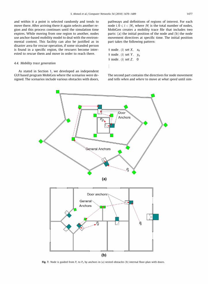
As stated in Section 1, we developed an independentGUI based program MobiGen where the scenarios were de-signed. The scenarios include various obstacles with doors,

Fig. 7. Node is guided from Ps to Pd by anchors in (a) ne

pathways and definitions of regions of interest. For eachnode i;0 6 i < jNj, where jNj is the total number of nodes,MobiGen creates a mobility trace file that includes twoparts: (a) the initial position of the node and (b) the nodemovement directives at specific time. The initial positionpart takes the following pattern:

$ node ðiÞ set X x0

$ node ðiÞ set Y y0

$ node ðiÞ set Z 0

..

.

The second part contains the directives for node movementand tells when and where to move at what speed until sim-

sted obstacles (b) internal floor-plan with doors.

Table 3Notations used in computational complexity analysis.

Notation Meaning

k Number of obstaclesi Number of IGVe Number of EGVib Number of IGV of obstacle bdb Number of doors of obstacle bd Number of doorsp Number of PVw Number of walls, and general vertices in the scenariowb Number of walls of obstacle br Number of user defined roadsjNj Number of nodesT Simulation durationI Average number of destination

selection by a node withinsimulation time T


ulation duration T expires. This part takes the followingform:

$ ns at t0 \node ðiÞ setdest x1 y1 s1"

$ ns at t1 \node ðiÞ setdest x2 y2 s2"

..

.

$ ns at tj \node ðiÞ setdest xjþ1 yjþ1 sjþ1"

where j P 0 and tj 6 T. This implies, an arbitrary node iwill start to move at time t0 to destination ðx1; y1Þ withspeed s1. After arriving there it pauses for pause time tp iftp > 0. Thus tlþ1 is calculated recursively as:

tlþ1 ¼ tl þ

ffiffiffiffiffiffiffiffiffiffiffiffiffiffiffiffiffiffiffiffiffiffiffiffiffiffiffiffiffiffiffiffiffiffiffiffiffiffiffiffiffiffiffiffiffiffiffiffiffiffiffiffiðxlþ1 � xlÞ2 þ ðylþ1 � ylÞ

2q

slþ1þ tp: ð1Þ

where 0 6 l < j. After generating the mobility trace file, itit attached to ns2 as scenario file. The scheduler in ns2schedules each of the events and executes when theappropriate time comes. Thus nodes move according tothe directives specified in the file starting from the initialpositions based on the various scenarios generated byAMM.

4.5. Applicability of AMM

It is obvious that there can be no single mobility modelthat is the best for every terrain. Our proposed mobilitymodel is focused to mimic the movement of people in pe-destrian friendly area (e.g., university/school campus, tech-no park), where people can move anywhere except theinaccessible obstacles in the specified area with the free-dom and flexibility of using/not using existing pathways.By following the generated graph considering anchors, itis possible to move anywhere in the terrain without collid-ing with the wall of obstacles. AMM assumes people to beaware of the exact position of obstacles, doors and path-ways. This model can also support nested obstacles (obsta-cles within obstacle) at any level as well as internal floor-plan for a building as shown in Fig. 7. However, the pro-posed mobility model may not be suitable in environmentslike City mobility where one mobile entity’s mobility is af-fected by other entities and needs modification. It can beinferred that AMM is a specialized Random Waypointmodel that can adopt various geographic attributes. Ifthere is no obstacle and pathway, no anchor is needed tobe generated and the model turns into simple RandomWaypoint model.

5. Computational complexity

In this Section, we present the computational complex-ity of our proposed mobility model. Table 3 illustrates thenotations used for this analysis.

It can be inferred that the total number of corner pointsof obstacles = the total number of walls = w. So, w generalanchors ðw ¼ ðiþ eÞÞ are placed at the corners of eachobstacle, either inside or outside. An IDV and EDV are gen-erated for each door. As a result, total number of IDV = to-tal number of EDV = d. Again, finding intersection of two

lines and adjustWeightð Þ function in Algorithm 1 have con-stant time complexity. For anchor computation each gen-eral anchor is tested whether it intersects with anyobstacles. Finding intersection in brute force method oftwo polygons needs OðmnÞ computation [33], where mand n denote the number of corners of each polygon,respectively. For our model where anchors have fixednumber of (four) corner points, the complexity becomesOð4mÞ ¼ OðmÞ. Resizing of anchors after finding intersec-tion requires constant time. Then the complexity for com-puting general anchors is:

Xk

b¼1

OðwbÞ ! Xk

b¼1

wb

!¼ Oðw2Þ; ð2Þ

sincePk

b¼1wb ¼ w. As doorway and pathway anchors areuser defined, it can be reasonably assumed that theywill not intersect with any obstacle, making thecomplexity

Oðw2 þ 2dþ pÞ ¼ Oðw2 þ dþ pÞ: ð3Þ

Step 1 in Algorithm 1 generates OðdÞ þ OPk

b¼1db þ ib

2

� ��

edges and OPk

b¼1db þ ib

2

� �� edges need to be checked

for intersection walls of respective obstacles resulting

OðdÞ þ OXk

b¼1

db þ ib

2

� �wb

!6 Oðdþ kwmaxðdmax þ imaxÞ2Þ;

ð4Þ

where wmax; dmax and imax are maximum values of wb; db

and ib, respectively, for all values of b.In step 2, each edge is checked with every wall for inter-

section requiring:

eþ dþ p

2

� ��

p

2

� �� Xk

b¼1

wb 6 Oðwðeþ dþ pÞ2Þ:

ð5Þ

Step 3 requires

OðrÞ: ð6Þ

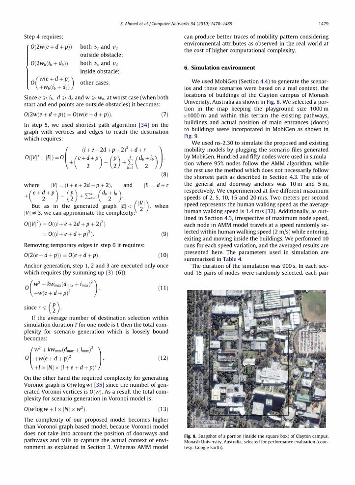
Fig. 8. Snapshot of a portion (inside the square box) of Clayton campus,Monash University, Australia, selected for performance evaluation (cour-tesy: Google Earth).


Step 4 requires:

Oð2wðeþ dþ pÞÞ both v s and vd

outside obstacle;Oð2wbðib þ dbÞÞ both v s and vd

inside obstacle;

Owðeþ dþ pÞþwbðib þ dbÞ

� �other cases:

8>>>>>>>><>>>>>>>>:Since e P ib; d P db and w P wb, at worst case (when bothstart and end points are outside obstacles) it becomes:

Oð2wðeþ dþ pÞÞ ¼ Oðwðeþ dþ pÞÞ: ð7Þ

In step 5, we used shortest path algorithm [34] on thegraph with vertices and edges to reach the destinationwhich requires:

OðjV j2þjEjÞ ¼Oðiþ eþ2dþpþ2Þ2þdþ r

þeþdþp

2

� ��

p

2

� �þPkb¼1

dbþ ib

2

� �0B@

1CA;ð8Þ

where jV j ¼ ðiþ eþ 2dþ pþ 2Þ, and jEj ¼ dþ r

þ eþ dþ p2

� �� p

2

� �þPk

b¼1db þ ib

2

� �.

But as in the generated graph jEj < jV j2

� �, when

jV j– 3, we can approximate the complexity:

OðjV j2Þ ¼ Oððiþ eþ 2dþ pþ 2Þ2Þ

¼ Oððiþ eþ dþ pÞ2Þ: ð9Þ

Removing temporary edges in step 6 it requires:

Oð2ðeþ dþ pÞÞ ¼ Oðeþ dþ pÞ: ð10Þ

Anchor generation, step 1, 2 and 3 are executed only oncewhich requires (by summing up (3)–(6)):

Ow2 þ kwmaxðdmax þ imaxÞ2

þwðeþ dþ pÞ2

!; ð11Þ

since r 6p2

� �.

If the average number of destination selection withinsimulation duration T for one node is I, then the total com-plexity for scenario generation which is loosely boundbecomes:

O

w2 þ kwmaxðdmax þ imaxÞ2

þwðeþ dþ pÞ2

þI � jNj � ðiþ eþ dþ pÞ2

0B@

1CA: ð12Þ

On the other hand the required complexity for generatingVoronoi graph is Oðw log wÞ [35] since the number of gen-erated Voronoi vertices is OðwÞ. As a result the total com-plexity for scenario generation in Voronoi model is:

Oðw log wþ I � jNj �w2Þ: ð13Þ

The complexity of our proposed model becomes higherthan Voronoi graph based model, because Voronoi modeldoes not take into account the position of doorways andpathways and fails to capture the actual context of envi-ronment as explained in Section 3. Whereas AMM model

can produce better traces of mobility pattern consideringenvironmental attributes as observed in the real world atthe cost of higher computational complexity.

6. Simulation environment

We used MobiGen (Section 4.4) to generate the scenar-ios and these scenarios were based on a real context, thelocations of buildings of the Clayton campus of MonashUniversity, Australia as shown in Fig. 8. We selected a por-tion in the map keeping the playground size 1000 m�1000 m and within this terrain the existing pathways,buildings and actual position of main entrances (doors)to buildings were incorporated in MobiGen as shown inFig. 9.

We used ns-2.30 to simulate the proposed and existingmobility models by plugging the scenario files generatedby MobiGen. Hundred and fifty nodes were used in simula-tion where 95% nodes follow the AMM algorithm, whilethe rest use the method which does not necessarily followthe shortest path as described in Section 4.3. The side ofthe general and doorway anchors was 10 m and 5 m,respectively. We experimented at five different maximumspeeds of 2, 5, 10, 15 and 20 m/s. Two meters per secondspeed represents the human walking speed as the averagehuman walking speed is 1.4 m/s [32]. Additionally, as out-lined in Section 4.3, irrespective of maximum node speed,each node in AMM model travels at a speed randomly se-lected within human walking speed (2 m/s) while entering,exiting and moving inside the buildings. We performed 10runs for each speed variation, and the averaged results arepresented here. The parameters used in simulation aresummarized in Table 4.

The duration of the simulation was 900 s. In each sec-ond 15 pairs of nodes were randomly selected, each pair

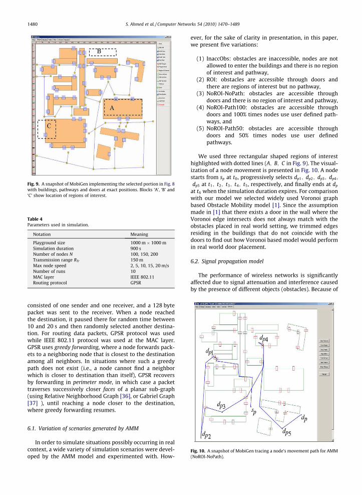
Fig. 9. A snapshot of MobiGen implementing the selected portion in Fig. 8with buildings, pathways and doors at exact positions. Blocks ‘A’, ‘B’ and‘C’ show location of regions of interest.

Table 4Parameters used in simulation.

Notation Meaning

Playground size 1000 m � 1000 mSimulation duration 900 sNumber of nodes N 100, 150, 200Transmission range RTr 150 mMax node speed 2, 5, 10, 15, 20 m/sNumber of runs 10MAC layer IEEE 802.11Routing protocol GPSR


consisted of one sender and one receiver, and a 128 bytepacket was sent to the receiver. When a node reachedthe destination, it paused there for random time between10 and 20 s and then randomly selected another destina-tion. For routing data packets, GPSR protocol was usedwhile IEEE 802.11 protocol was used at the MAC layer.GPSR uses greedy forwarding, where a node forwards pack-ets to a neighboring node that is closest to the destinationamong all neighbors. In situations where such a greedypath does not exist (i.e., a node cannot find a neighborwhich is closer to destination than itself), GPSR recoversby forwarding in perimeter mode, in which case a packettraverses successively closer faces of a planar sub-graph(using Relative Neighborhood Graph [36], or Gabriel Graph[37] ), until reaching a node closer to the destination,where greedy forwarding resumes.

Fig. 10. A snapshot of MobiGen tracing a node’s movement path for AMM(NoROI-NoPath).

6.1. Variation of scenarios generated by AMM

In order to simulate situations possibly occurring in realcontext, a wide variety of simulation scenarios were devel-oped by the AMM model and experimented with. How-

ever, for the sake of clarity in presentation, in this paper,we present five variations:

(1) InaccObs: obstacles are inaccessible, nodes are notallowed to enter the buildings and there is no regionof interest and pathway,

(2) ROI: obstacles are accessible through doors andthere are regions of interest but no pathway,

(3) NoROI-NoPath: obstacles are accessible throughdoors and there is no region of interest and pathway,

(4) NoROI-Path100: obstacles are accessible throughdoors and 100% times nodes use user defined path-ways, and

(5) NoROI-Path50: obstacles are accessible throughdoors and 50% times nodes use user definedpathways.

We used three rectangular shaped regions of interesthighlighted with dotted lines (A; B; C in Fig. 9). The visual-ization of a node movement is presented in Fig. 10. A nodestarts from sp at t0, progressively selects dp1; dp2; dp3; dp4;

dp5 at t1; t2; t3; t4; t5, respectively, and finally ends at dp

at t6 when the simulation duration expires. For comparisonwith our model we selected widely used Voronoi graphbased Obstacle Mobility model [1]. Since the assumptionmade in [1] that there exists a door in the wall where theVoronoi edge intersects does not always match with theobstacles placed in real world setting, we trimmed edgesresiding in the buildings that do not coincide with thedoors to find out how Voronoi based model would performin real world door placement.

6.2. Signal propagation model

The performance of wireless networks is significantlyaffected due to signal attenuation and interference causedby the presence of different objects (obstacles). Because of

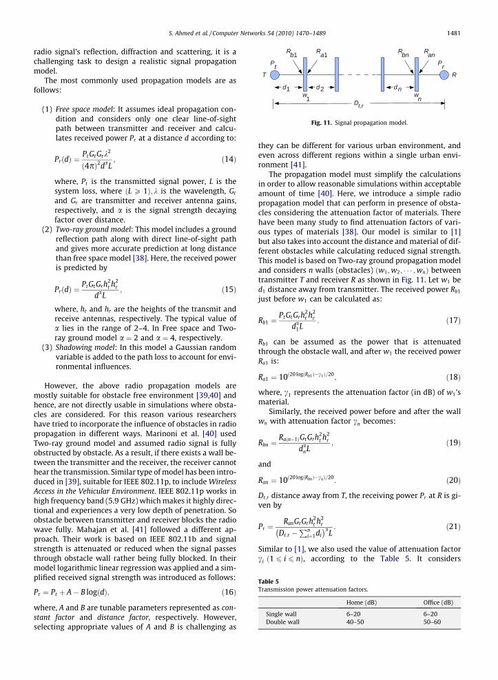
Fig. 11. Signal propagation model.


radio signal’s reflection, diffraction and scattering, it is achallenging task to design a realistic signal propagationmodel.

The most commonly used propagation models are asfollows:

(1) Free space model: It assumes ideal propagation con-dition and considers only one clear line-of-sightpath between transmitter and receiver and calcu-lates received power Pr at a distance d according to:

PrðdÞ ¼PtGtGrk

2

ð4pÞ2daL; ð14Þ

where, Pt is the transmitted signal power, L is thesystem loss, where ðL P 1Þ; k is the wavelength, Gt

and Gr are transmitter and receiver antenna gains,respectively, and a is the signal strength decayingfactor over distance.

(2) Two-ray ground model: This model includes a groundreflection path along with direct line-of-sight pathand gives more accurate prediction at long distancethan free space model [38]. Here, the received poweris predicted by

PrðdÞ ¼PtGtGrh

2t h2

r

daL; ð15Þ

where, ht and hr are the heights of the transmit andreceive antennas, respectively. The typical value ofa lies in the range of 2–4. In Free space and Two-ray ground model a ¼ 2 and a ¼ 4, respectively.

Table 5Transmission power attenuation factors.

Home (dB) Office (dB)

Single wall 6–20 6–20Double wall 40–50 50–60

(3) Shadowing model: In this model a Gaussian randomvariable is added to the path loss to account for envi-ronmental influences.

However, the above radio propagation models aremostly suitable for obstacle free environment [39,40] andhence, are not directly usable in simulations where obsta-cles are considered. For this reason various researchershave tried to incorporate the influence of obstacles in radiopropagation in different ways. Marinoni et al. [40] usedTwo-ray ground model and assumed radio signal is fullyobstructed by obstacle. As a result, if there exists a wall be-tween the transmitter and the receiver, the receiver cannothear the transmission. Similar type of model has been intro-duced in [39], suitable for IEEE 802.11p, to include WirelessAccess in the Vehicular Environment. IEEE 802.11p works inhigh frequency band (5.9 GHz) which makes it highly direc-tional and experiences a very low depth of penetration. Soobstacle between transmitter and receiver blocks the radiowave fully. Mahajan et al. [41] followed a different ap-proach. Their work is based on IEEE 802.11b and signalstrength is attenuated or reduced when the signal passesthrough obstacle wall rather being fully blocked. In theirmodel logarithmic linear regression was applied and a sim-plified received signal strength was introduced as follows:

Pr ¼ Pt þ A� B logðdÞ; ð16Þ

where, A and B are tunable parameters represented as con-stant factor and distance factor, respectively. However,selecting appropriate values of A and B is challenging as

they can be different for various urban environment, andeven across different regions within a single urban envi-ronment [41].

The propagation model must simplify the calculationsin order to allow reasonable simulations within acceptableamount of time [40]. Here, we introduce a simple radiopropagation model that can perform in presence of obsta-cles considering the attenuation factor of materials. Therehave been many study to find attenuation factors of vari-ous types of materials [38]. Our model is similar to [1]but also takes into account the distance and material of dif-ferent obstacles while calculating reduced signal strength.This model is based on Two-ray ground propagation modeland considers n walls (obstacles) ðw1;w2; � � � ;wnÞ betweentransmitter T and receiver R as shown in Fig. 11. Let w1 bed1 distance away from transmitter. The received power Rb1

just before w1 can be calculated as:

Rb1 ¼PtGtGrh

2t h2

r

da1L

: ð17Þ

Rb1 can be assumed as the power that is attenuatedthrough the obstacle wall, and after w1 the received powerRa1 is:

Ra1 ¼ 10ð20 logðRb1Þ�c1Þ=20; ð18Þ

where, c1 represents the attenuation factor (in dB) of w1’smaterial.

Similarly, the received power before and after the wallwn with attenuation factor cn becomes:

Rbn ¼Raðn�1ÞGtGrh

2t h2

r

danL

; ð19Þ

and

Ran ¼ 10ð20 logðRbnÞ�cnÞ=20: ð20Þ

Dt;r distance away from T, the receiving power Pr at R is gi-ven by

Pr ¼RanGtGrh

2t h2

r

Dt;r �Pn

i¼1di� �aL

: ð21Þ

Similar to [1], we also used the value of attenuation factorci ð1 6 i 6 nÞ, according to the Table 5. It considers

100 200 300 400 500 600 700 800 9006

8

10

12

14

16

18

20

22

24

Time(sec)

Num

ber o

f nei

ghbo

rs

ROIInaccObsNoROI−Path50NoROI−NoPathNoROI−Path100Voronoi

Fig. 12. Variation of average number of neighbors over time (at 10 m/s).

2 5 10 15 208

10

12

14

16

18

20

22

Max speed (m/sec)

Num

ber o

f nei

ghbo

rsROIInaccObsNoROI−Path50NoROI−NoPathNoROI−Path100Voronoi

Fig. 13. Average number of neighbors.

2 5 10 15 208

10

12

14

16

18

20

22

24

Max speed (m/sec)

Num

ber o

f nei

ghbo

rs

ROIInaccObsNoROI−Path50NoROI−NoPathNoROI−Path100Voronoi

Fig. 14. Average number of neighbors without considering signalattenuation.


whether the signal penetrates through a single or doublewall in a home or office. Since we are modeling a universitycampus, only the attenuation factors for office are consid-ered. We considered only boundary walls of obstacles asshown in Fig. 9.

The formula to calculate the received signal strength isreported in (22). In particular, the equation is exactly thesame as Two-ray ground model when no obstacle is pres-ent between transmitter and receiver, and (21) is usedelsewhere that eventually reduces the signal strengthaccording to the distance and attenuation factor of eachwall that exists between transmitter and receiver.

Pr ¼

Pt Gt Gr h2t h2

rDa

t;r L no obstruction;

RanGt Gr h2t h2

r

Dt;r�Pn

i¼1di

� �aL

elsewhere:

8><>: ð22Þ

To recognize the signal, Pr must fulfill Pr P Rx, where Rx

represents the minimum signal threshold required to re-ceive the signal successfully. In our simulations we se-lected a ¼ 4. In this way this propagation modelintroduces partially pass radio signal through obstacles.

7. Simulation results

Various network performance parameters are calcu-lated which includes: (a) number of neighbors at differenttime span and speed, (b) link duration, (c) path length be-tween packet originator and receiver in terms of hops, (d)packet delivery success rate at different node speed anddensity, (e) end to end delay, and (f) routing overhead.These measures are also investigated in simulation of sim-ilar studies [1,6]. We used the propagation model as de-fined in ns-2.30 with signal attenuation as described inSection 6.2. Moreover, we also repeated the same experi-ment without considering signal attenuation in order toinvestigate the impact of signal attenuation on networkperformance. Unless otherwise stated, signal attenuationis considered in the simulation presented below. Distribu-tion of nodes and partition formation in mobility modelsand their characteristics in large area are also investigated.

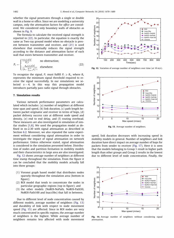
Fig. 12 shows average number of neighbors at differenttime stamp throughout the simulation. From the figure itcan be concluded that the mobility models actually fallinto three groups:

(1) Voronoi graph based model that distributes nodessparsely throughout the simulation area (bottom infigure);

(2) ROI model that tends to concentrate the nodes inparticular geographic regions (top in figure); and

(3) the other models (NoROI-NoPath, NoROI-Path50,NoROI-Path100 and InaccObs) that fall in between.

Due to different level of node concentration caused bydifferent models, average number of neighbors (Fig. 13)and durability of link with respect to node movementspeed (Fig. 15) are affected. Since in ROI nodes are verymuch concentrated in specific regions, the average numberof neighbors is the highest. While average number ofneighbors remains less affected with node movement

speed, link duration decreases with increasing speed inmobility models in general. Number of neighbors and linkduration have direct impact on average number of hops forpackets from sender to receiver (Fig. 17). Here it is seenthat the models belonging to Group 1 result in higher pathlength than other groups and Group 2 results in the lowestdue to different level of node concentration. Finally, the

2 5 10 15 2020

30

40

50

60

70

80

Max speed (m/sec)

Link

dur

atio

n(se

c)

ROINoROI−NoPathNoROI−Path100NoROI−Path50InaccObsVoronoi

Fig. 16. Average link duration without considering signal attenuation.


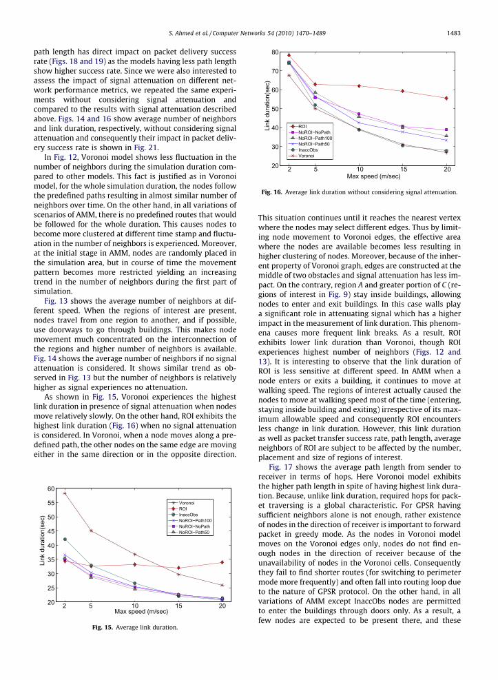
path length has direct impact on packet delivery successrate (Figs. 18 and 19) as the models having less path lengthshow higher success rate. Since we were also interested toassess the impact of signal attenuation on different net-work performance metrics, we repeated the same experi-ments without considering signal attenuation andcompared to the results with signal attenuation describedabove. Figs. 14 and 16 show average number of neighborsand link duration, respectively, without considering signalattenuation and consequently their impact in packet deliv-ery success rate is shown in Fig. 21.

In Fig. 12, Voronoi model shows less fluctuation in thenumber of neighbors during the simulation duration com-pared to other models. This fact is justified as in Voronoimodel, for the whole simulation duration, the nodes followthe predefined paths resulting in almost similar number ofneighbors over time. On the other hand, in all variations ofscenarios of AMM, there is no predefined routes that wouldbe followed for the whole duration. This causes nodes tobecome more clustered at different time stamp and fluctu-ation in the number of neighbors is experienced. Moreover,at the initial stage in AMM, nodes are randomly placed inthe simulation area, but in course of time the movementpattern becomes more restricted yielding an increasingtrend in the number of neighbors during the first part ofsimulation.

Fig. 13 shows the average number of neighbors at dif-ferent speed. When the regions of interest are present,nodes travel from one region to another, and if possible,use doorways to go through buildings. This makes nodemovement much concentrated on the interconnection ofthe regions and higher number of neighbors is available.Fig. 14 shows the average number of neighbors if no signalattenuation is considered. It shows similar trend as ob-served in Fig. 13 but the number of neighbors is relativelyhigher as signal experiences no attenuation.

As shown in Fig. 15, Voronoi experiences the highestlink duration in presence of signal attenuation when nodesmove relatively slowly. On the other hand, ROI exhibits thehighest link duration (Fig. 16) when no signal attenuationis considered. In Voronoi, when a node moves along a pre-defined path, the other nodes on the same edge are movingeither in the same direction or in the opposite direction.

2 5 10 15 2020

25

30

35

40

45

50

55

60

Max speed (m/sec)

Link

dur

atio

n(se

c)

VoronoiROIInaccObsNoROI−Path100NoROI−NoPathNoROI−Path50

Fig. 15. Average link duration.

This situation continues until it reaches the nearest vertexwhere the nodes may select different edges. Thus by limit-ing node movement to Voronoi edges, the effective areawhere the nodes are available becomes less resulting inhigher clustering of nodes. Moreover, because of the inher-ent property of Voronoi graph, edges are constructed at themiddle of two obstacles and signal attenuation has less im-pact. On the contrary, region A and greater portion of C (re-gions of interest in Fig. 9) stay inside buildings, allowingnodes to enter and exit buildings. In this case walls playa significant role in attenuating signal which has a higherimpact in the measurement of link duration. This phenom-ena causes more frequent link breaks. As a result, ROIexhibits lower link duration than Voronoi, though ROIexperiences highest number of neighbors (Figs. 12 and13). It is interesting to observe that the link duration ofROI is less sensitive at different speed. In AMM when anode enters or exits a building, it continues to move atwalking speed. The regions of interest actually caused thenodes to move at walking speed most of the time (entering,staying inside building and exiting) irrespective of its max-imum allowable speed and consequently ROI encountersless change in link duration. However, this link durationas well as packet transfer success rate, path length, averageneighbors of ROI are subject to be affected by the number,placement and size of regions of interest.

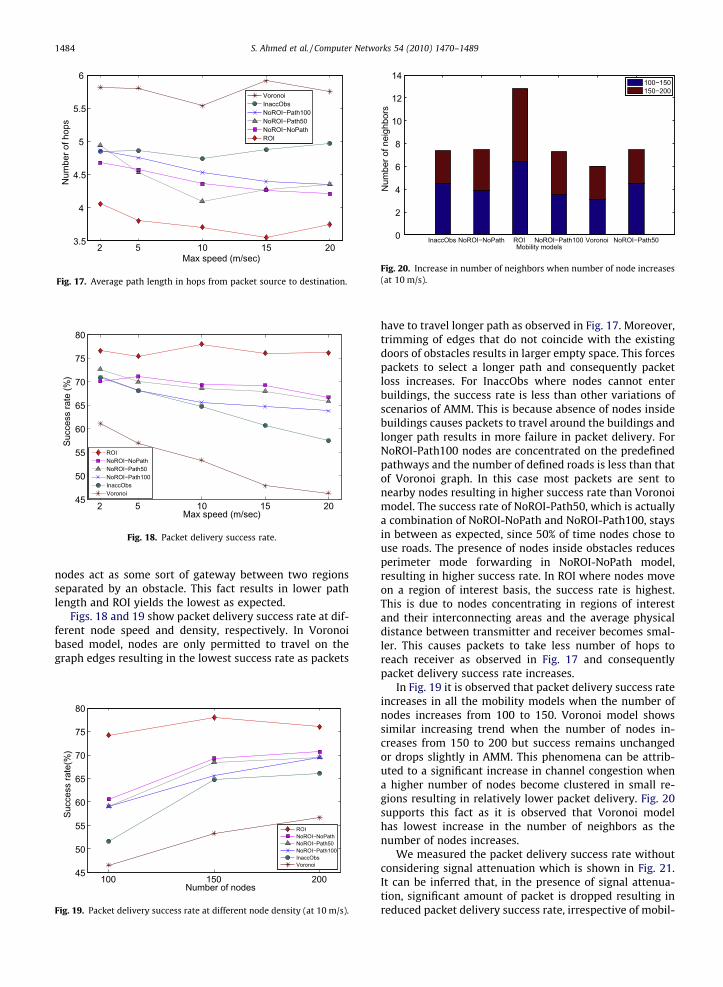
Fig. 17 shows the average path length from sender toreceiver in terms of hops. Here Voronoi model exhibitsthe higher path length in spite of having highest link dura-tion. Because, unlike link duration, required hops for pack-et traversing is a global characteristic. For GPSR havingsufficient neighbors alone is not enough, rather existenceof nodes in the direction of receiver is important to forwardpacket in greedy mode. As the nodes in Voronoi modelmoves on the Voronoi edges only, nodes do not find en-ough nodes in the direction of receiver because of theunavailability of nodes in the Voronoi cells. Consequentlythey fail to find shorter routes (for switching to perimetermode more frequently) and often fall into routing loop dueto the nature of GPSR protocol. On the other hand, in allvariations of AMM except InaccObs nodes are permittedto enter the buildings through doors only. As a result, afew nodes are expected to be present there, and these

2 5 10 15 203.5

4

4.5

5

5.5

6

Max speed (m/sec)

Num

ber o

f hop

s

VoronoiInaccObsNoROI−Path100NoROI−Path50NoROI−NoPathROI

Fig. 17. Average path length in hops from packet source to destination.

2 5 10 15 2045

50

55

60

65

70

75

80

Max speed (m/sec)

Succ

ess

rate

(%)


Fig. 18. Packet delivery success rate.

InaccObs NoROI−NoPath ROI NoROI−Path100 Voronoi NoROI−Path500

2

4

6

8

10

12

14

Mobility models

Num

ber o

f nei

ghbo

rs

100−150150−200

Fig. 20. Increase in number of neighbors when number of node increases(at 10 m/s).


nodes act as some sort of gateway between two regionsseparated by an obstacle. This fact results in lower pathlength and ROI yields the lowest as expected.

Figs. 18 and 19 show packet delivery success rate at dif-ferent node speed and density, respectively. In Voronoibased model, nodes are only permitted to travel on thegraph edges resulting in the lowest success rate as packets

100 150 20045

50

55

60

65

70

75

80

Number of nodes

Succ

ess

rate

(%)


Fig. 19. Packet delivery success rate at different node density (at 10 m/s).

have to travel longer path as observed in Fig. 17. Moreover,trimming of edges that do not coincide with the existingdoors of obstacles results in larger empty space. This forcespackets to select a longer path and consequently packetloss increases. For InaccObs where nodes cannot enterbuildings, the success rate is less than other variations ofscenarios of AMM. This is because absence of nodes insidebuildings causes packets to travel around the buildings andlonger path results in more failure in packet delivery. ForNoROI-Path100 nodes are concentrated on the predefinedpathways and the number of defined roads is less than thatof Voronoi graph. In this case most packets are sent tonearby nodes resulting in higher success rate than Voronoimodel. The success rate of NoROI-Path50, which is actuallya combination of NoROI-NoPath and NoROI-Path100, staysin between as expected, since 50% of time nodes chose touse roads. The presence of nodes inside obstacles reducesperimeter mode forwarding in NoROI-NoPath model,resulting in higher success rate. In ROI where nodes moveon a region of interest basis, the success rate is highest.This is due to nodes concentrating in regions of interestand their interconnecting areas and the average physicaldistance between transmitter and receiver becomes smal-ler. This causes packets to take less number of hops toreach receiver as observed in Fig. 17 and consequentlypacket delivery success rate increases.

In Fig. 19 it is observed that packet delivery success rateincreases in all the mobility models when the number ofnodes increases from 100 to 150. Voronoi model showssimilar increasing trend when the number of nodes in-creases from 150 to 200 but success remains unchangedor drops slightly in AMM. This phenomena can be attrib-uted to a significant increase in channel congestion whena higher number of nodes become clustered in small re-gions resulting in relatively lower packet delivery. Fig. 20supports this fact as it is observed that Voronoi modelhas lowest increase in the number of neighbors as thenumber of nodes increases.

We measured the packet delivery success rate withoutconsidering signal attenuation which is shown in Fig. 21.It can be inferred that, in the presence of signal attenua-tion, significant amount of packet is dropped resulting inreduced packet delivery success rate, irrespective of mobil-

2 5 10 15 2060

65

70

75

80

85

90

95

Max speed (m/sec)

Succ

ess

rate

(%)


Fig. 21. Packet delivery success rate without considering signalattenuation.


ity models as a comparison between Figs. 18 and 21 re-veals. It can be concluded that while using models belong-ing to Group 2, the routing protocol has the highest successrate, whereas with Group 1 it performs lowest, and forGroup 3 the success rate stays in between.

To test the significance of difference in success rateamong models (Fig. 18), we selected InaccObs and Voronoias representatives of the proposed AMM models and exist-ing models, respectively. The t-test at speed 2, 5, 10, 15 and20 m/s yielded p-values of p < 2:11� 10�8; 4:79� 10�7;

0

2

4

6

8

Num

ber o

f nod

es

0

1

2

3

4

Num

ber o

f nod

es

(a) (b)

(d) (e)

Fig. 22. Node distribution in the playground and it contour plot, respectively,number of nodes in the playground is 200.

4:10� 10�7; 1:30� 10�6; 9:24� 10�6 at 99% confidencelevel, validating their performance difference being statis-tically significant.

7.1. Distribution of nodes

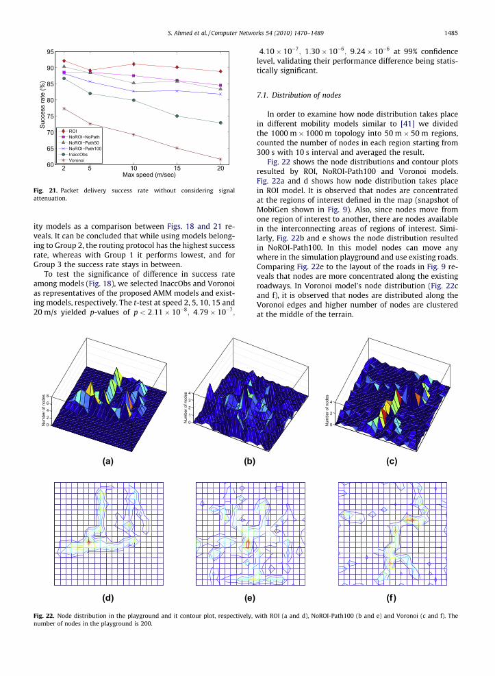
In order to examine how node distribution takes placein different mobility models similar to [41] we dividedthe 1000 m� 1000 m topology into 50 m� 50 m regions,counted the number of nodes in each region starting from300 s with 10 s interval and averaged the result.

Fig. 22 shows the node distributions and contour plotsresulted by ROI, NoROI-Path100 and Voronoi models.Fig. 22a and d shows how node distribution takes placein ROI model. It is observed that nodes are concentratedat the regions of interest defined in the map (snapshot ofMobiGen shown in Fig. 9). Also, since nodes move fromone region of interest to another, there are nodes availablein the interconnecting areas of regions of interest. Simi-larly, Fig. 22b and e shows the node distribution resultedin NoROI-Path100. In this model nodes can move anywhere in the simulation playground and use existing roads.Comparing Fig. 22e to the layout of the roads in Fig. 9 re-veals that nodes are more concentrated along the existingroadways. In Voronoi model’s node distribution (Fig. 22cand f), it is observed that nodes are distributed along theVoronoi edges and higher number of nodes are clusteredat the middle of the terrain.

0

2

4

Num

ber o

f nod

es

(c)

(f)

with ROI (a and d), NoROI-Path100 (b and e) and Voronoi (c and f). The


In presence of regions of interest, AMM variation of ROIcreates those regions centric node distribution which re-flects what happens in real world, as it is observed thatwhen there are regions of interest, people intent to gothere and node density becomes higher in regions of inter-est. In presence of existing roads, people tend to use roadsresulting in more density along the roadways and this realworld experience is representable through NoROI-Path100variation. Thus it can be concluded that AMM is flexible en-ough to cater various situations by considering environ-mental context more realistically while directing nodemobility resulting in node distribution to be similar to thatof real-world scenario.

7.2. Protocol overhead and packet delivery delay

Figs. 23 and 24 represent the end to end delay and rout-ing overhead, respectively. Increased MAC layer congestioncauses ROI to encounter higher end to end delay as shownin Fig. 23 though ROI requires lower path length (Fig. 17).Since in Voronoi nodes only move on Voronoi edges, lowerchannel congestion is observed and consequently end toend delay becomes lower. Having the concentration levelof nodes more than that of Voronoi and less than that of

100 150 2000

0.2

0.4

0.6

0.8

1

1.2

1.4

Number of nodes

End

to e

nd d

elay

(sec

)


Fig. 23. End to end delay for packet delivery.

2 5 10 15 200.96

0.98

1

1.02

1.04

1.06

1.08 x 105

Max speed (m/sec)

Rou

ting

over

head

(pac

ket)

ROINoROI−Path50NoROI−Path100NoROI−NoPathInaccObsVoronoi

Fig. 24. Routing overhead.

ROI, the end to end delay of other variations of AMM staysin between.

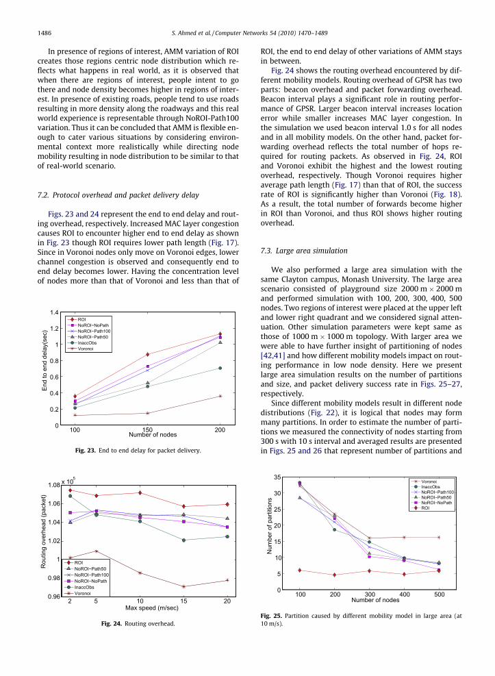
Fig. 24 shows the routing overhead encountered by dif-ferent mobility models. Routing overhead of GPSR has twoparts: beacon overhead and packet forwarding overhead.Beacon interval plays a significant role in routing perfor-mance of GPSR. Larger beacon interval increases locationerror while smaller increases MAC layer congestion. Inthe simulation we used beacon interval 1.0 s for all nodesand in all mobility models. On the other hand, packet for-warding overhead reflects the total number of hops re-quired for routing packets. As observed in Fig. 24, ROIand Voronoi exhibit the highest and the lowest routingoverhead, respectively. Though Voronoi requires higheraverage path length (Fig. 17) than that of ROI, the successrate of ROI is significantly higher than Voronoi (Fig. 18).As a result, the total number of forwards become higherin ROI than Voronoi, and thus ROI shows higher routingoverhead.

7.3. Large area simulation

We also performed a large area simulation with thesame Clayton campus, Monash University. The large areascenario consisted of playground size 2000 m� 2000 mand performed simulation with 100, 200, 300, 400, 500nodes. Two regions of interest were placed at the upper leftand lower right quadrant and we considered signal atten-uation. Other simulation parameters were kept same asthose of 1000 m� 1000 m topology. With larger area wewere able to have further insight of partitioning of nodes[42,41] and how different mobility models impact on rout-ing performance in low node density. Here we presentlarge area simulation results on the number of partitionsand size, and packet delivery success rate in Figs. 25–27,respectively.

Since different mobility models result in different nodedistributions (Fig. 22), it is logical that nodes may formmany partitions. In order to estimate the number of parti-tions we measured the connectivity of nodes starting from300 s with 10 s interval and averaged results are presentedin Figs. 25 and 26 that represent number of partitions and

100 200 300 400 5000

5

10

15

20

25

30

35

Number of nodes

Num

ber o

f par

titio

ns

VoronoiInaccObsNoROI−Path100NoROI−Path50NoROI−NoPathROI

Fig. 25. Partition caused by different mobility model in large area (at10 m/s).

ROINoROI−NoPath

InaccObsNoROI−Path100

NoROI−Path50Voronoi

100

200

300

400

500

020406080

100120

Number of nodes

Parti

tion

size

(nod

es)

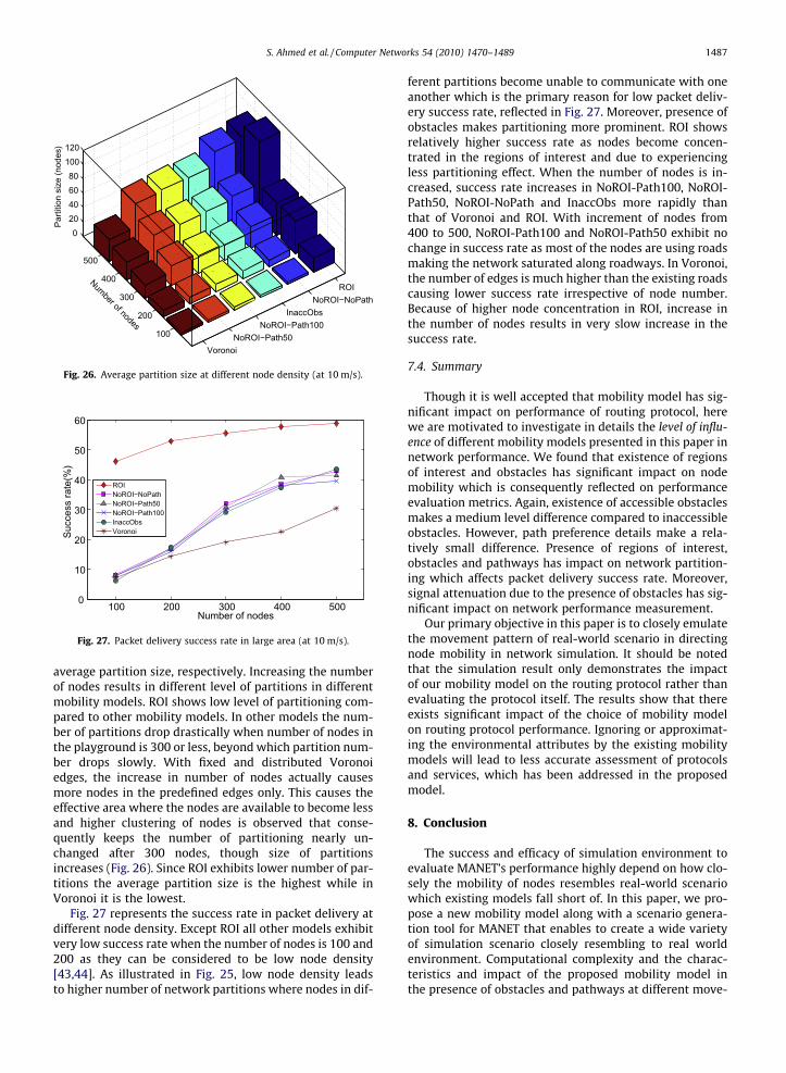
Fig. 26. Average partition size at different node density (at 10 m/s).

100 200 300 400 5000

10

20

30

40

50

60

Number of nodes

Succ

ess

rate

(%)


Fig. 27. Packet delivery success rate in large area (at 10 m/s).


average partition size, respectively. Increasing the numberof nodes results in different level of partitions in differentmobility models. ROI shows low level of partitioning com-pared to other mobility models. In other models the num-ber of partitions drop drastically when number of nodes inthe playground is 300 or less, beyond which partition num-ber drops slowly. With fixed and distributed Voronoiedges, the increase in number of nodes actually causesmore nodes in the predefined edges only. This causes theeffective area where the nodes are available to become lessand higher clustering of nodes is observed that conse-quently keeps the number of partitioning nearly un-changed after 300 nodes, though size of partitionsincreases (Fig. 26). Since ROI exhibits lower number of par-titions the average partition size is the highest while inVoronoi it is the lowest.

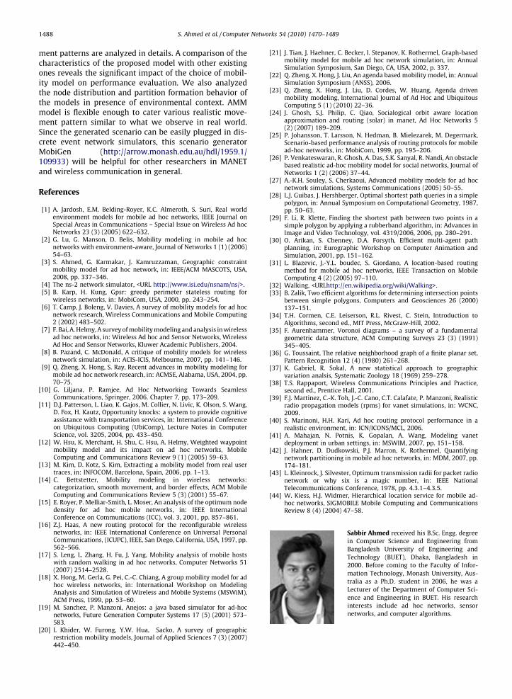
Fig. 27 represents the success rate in packet delivery atdifferent node density. Except ROI all other models exhibitvery low success rate when the number of nodes is 100 and200 as they can be considered to be low node density[43,44]. As illustrated in Fig. 25, low node density leadsto higher number of network partitions where nodes in dif-

ferent partitions become unable to communicate with oneanother which is the primary reason for low packet deliv-ery success rate, reflected in Fig. 27. Moreover, presence ofobstacles makes partitioning more prominent. ROI showsrelatively higher success rate as nodes become concen-trated in the regions of interest and due to experiencingless partitioning effect. When the number of nodes is in-creased, success rate increases in NoROI-Path100, NoROI-Path50, NoROI-NoPath and InaccObs more rapidly thanthat of Voronoi and ROI. With increment of nodes from400 to 500, NoROI-Path100 and NoROI-Path50 exhibit nochange in success rate as most of the nodes are using roadsmaking the network saturated along roadways. In Voronoi,the number of edges is much higher than the existing roadscausing lower success rate irrespective of node number.Because of higher node concentration in ROI, increase inthe number of nodes results in very slow increase in thesuccess rate.

7.4. Summary

Though it is well accepted that mobility model has sig-nificant impact on performance of routing protocol, herewe are motivated to investigate in details the level of influ-ence of different mobility models presented in this paper innetwork performance. We found that existence of regionsof interest and obstacles has significant impact on nodemobility which is consequently reflected on performanceevaluation metrics. Again, existence of accessible obstaclesmakes a medium level difference compared to inaccessibleobstacles. However, path preference details make a rela-tively small difference. Presence of regions of interest,obstacles and pathways has impact on network partition-ing which affects packet delivery success rate. Moreover,signal attenuation due to the presence of obstacles has sig-nificant impact on network performance measurement.

Our primary objective in this paper is to closely emulatethe movement pattern of real-world scenario in directingnode mobility in network simulation. It should be notedthat the simulation result only demonstrates the impactof our mobility model on the routing protocol rather thanevaluating the protocol itself. The results show that thereexists significant impact of the choice of mobility modelon routing protocol performance. Ignoring or approximat-ing the environmental attributes by the existing mobilitymodels will lead to less accurate assessment of protocolsand services, which has been addressed in the proposedmodel.

8. Conclusion

The success and efficacy of simulation environment toevaluate MANET’s performance highly depend on how clo-sely the mobility of nodes resembles real-world scenariowhich existing models fall short of. In this paper, we pro-pose a new mobility model along with a scenario genera-tion tool for MANET that enables to create a wide varietyof simulation scenario closely resembling to real worldenvironment. Computational complexity and the charac-teristics and impact of the proposed mobility model inthe presence of obstacles and pathways at different move-


ment patterns are analyzed in details. A comparison of thecharacteristics of the proposed model with other existingones reveals the significant impact of the choice of mobil-ity model on performance evaluation. We also analyzedthe node distribution and partition formation behavior ofthe models in presence of environmental context. AMMmodel is flexible enough to cater various realistic move-ment pattern similar to what we observe in real world.Since the generated scenario can be easily plugged in dis-crete event network simulators, this scenario generatorMobiGen (http://arrow.monash.edu.au/hdl/1959.1/109933) will be helpful for other researchers in MANETand wireless communication in general.

References

[1] A. Jardosh, E.M. Belding-Royer, K.C. Almeroth, S. Suri, Real worldenvironment models for mobile ad hoc networks, IEEE Journal onSpecial Areas in Communications – Special Issue on Wireless Ad hocNetworks 23 (3) (2005) 622–632.

[2] G. Lu, G. Manson, D. Belis, Mobility modeling in mobile ad hocnetworks with environment-aware, Journal of Networks 1 (1) (2006)54–63.

[3] S. Ahmed, G. Karmakar, J. Kamruzzaman, Geographic constraintmobility model for ad hoc network, in: IEEE/ACM MASCOTS, USA,2008, pp. 337–346.

[4] The ns-2 network simulator, <URL http://www.isi.edu/nsnam/ns/>.[5] B. Karp, H. Kung, Gpsr: greedy perimeter stateless routing for

wireless networks, in: MobiCom, USA, 2000, pp. 243–254.[6] T. Camp, J. Boleng, V. Davies, A survey of mobility models for ad hoc

network research, Wireless Communications and Mobile Computing2 (2002) 483–502.

[7] F. Bai, A. Helmy, A survey of mobility modeling and analysis in wirelessad hoc networks, in: Wireless Ad hoc and Sensor Networks, WirelessAd Hoc and Sensor Networks, Kluwer Academic Publishers, 2004.

[8] B. Pazand, C. McDonald, A critique of mobility models for wirelessnetwork simulation, in: ACIS-ICIS, Melbourne, 2007, pp. 141–146.

[9] Q. Zheng, X. Hong, S. Ray, Recent advances in mobility modeling formobile ad hoc network research, in: ACMSE, Alabama, USA, 2004, pp.70–75.

[10] G. Liljana, P. Ramjee, Ad Hoc Networking Towards SeamlessCommunications, Springer, 2006. Chapter 7, pp. 173–209.

[11] D.J. Patterson, L. Liao, K. Gajos, M. Collier, N. Livic, K. Olson, S. Wang,D. Fox, H. Kautz, Opportunity knocks: a system to provide cognitiveassistance with transportation services, in: International Conferenceon Ubiquitous Computing (UbiComp), Lecture Notes in ComputerScience, vol. 3205, 2004, pp. 433–450.

[12] W. Hsu, K. Merchant, H. Shu, C. Hsu, A. Helmy, Weighted waypointmobility model and its impact on ad hoc networks, MobileComputing and Communications Review 9 (1) (2005) 59–63.

[13] M. Kim, D. Kotz, S. Kim, Extracting a mobility model from real usertraces, in: INFOCOM, Barcelona, Spain, 2006, pp. 1–13.

[14] C. Bettstetter, Mobility modeling in wireless networks:categorization, smooth movement, and border effects, ACM MobileComputing and Communications Review 5 (3) (2001) 55–67.

[15] E. Royer, P. Melliar-Smith, L. Moser, An analysis of the optimum nodedensity for ad hoc mobile networks, in: IEEE InternationalConference on Communications (ICC), vol. 3, 2001, pp. 857–861.

[16] Z.J. Haas, A new routing protocol for the reconfigurable wirelessnetworks, in: IEEE International Conference on Universal PersonalCommunications, (ICUPC), IEEE, San Diego, California, USA, 1997, pp.562–566.

[17] S. Leng, L. Zhang, H. Fu, J. Yang, Mobility analysis of mobile hostswith random walking in ad hoc networks, Computer Networks 51(2007) 2514–2528.

[18] X. Hong, M. Gerla, G. Pei, C.-C. Chiang, A group mobility model for adhoc wireless networks, in: International Workshop on ModelingAnalysis and Simulation of Wireless and Mobile Systems (MSWiM),ACM Press, 1999, pp. 53–60.

[19] M. Sanchez, P. Manzoni, Anejos: a java based simulator for ad-hocnetworks, Future Generation Computer Systems 17 (5) (2001) 573–583.

[20] I. Khider, W. Furong, Y.W. Hua, Sacko, A survey of geographicrestriction mobility models, Journal of Applied Sciences 7 (3) (2007)442–450.

[21] J. Tian, J. Haehner, C. Becker, I. Stepanov, K. Rothermel, Graph-basedmobility model for mobile ad hoc network simulation, in: AnnualSimulation Symposium, San Diego, CA, USA, 2002, p. 337.

[22] Q. Zheng, X. Hong, J. Liu, An agenda based mobility model, in: AnnualSimulation Symposium (ANSS), 2006.

[23] Q. Zheng, X. Hong, J. Liu, D. Cordes, W. Huang, Agenda drivenmobility modeling, International Journal of Ad Hoc and UbiquitousComputing 5 (1) (2010) 22–36.

[24] J. Ghosh, S.J. Philip, C. Qiao, Socialogical orbit aware locationapproximation and routing (solar) in manet, Ad Hoc Networks 5(2) (2007) 189–209.

[25] P. Johansson, T. Larsson, N. Hedman, B. Mielezarek, M. Degermark,Scenario-based performance analysis of routing protocols for mobilead-hoc networks, in: MobiCom, 1999, pp. 195–206.

[26] P. Venkateswaran, R. Ghosh, A. Das, S.K. Sanyal, R. Nandi, An obstaclebased realistic ad-hoc mobility model for social networks, Journal ofNetworks 1 (2) (2006) 37–44.

[27] A.-K.H. Souley, S. Cherkaoui, Advanced mobility models for ad hocnetwork simulations, Systems Communications (2005) 50–55.

[28] L.J. Guibas, J. Hershberger, Optimal shortest path queries in a simplepolygon, in: Annual Symposium on Computational Geometry, 1987,pp. 50–63.

[29] F. Li, R. Klette, Finding the shortest path between two points in asimple polygon by applying a rubberband algorithm, in: Advances inImage and Video Technology, vol. 4319/2006, 2006, pp. 280–291.

[30] O. Arikan, S. Chenney, D.A. Forsyth, Efficient multi-agent pathplanning, in: Eurographic Workshop on Computer Animation andSimulation, 2001, pp. 151–162.

[31] L. Blazevic, J.-Y.L. boudec, S. Giordano, A location-based routingmethod for mobile ad hoc networks, IEEE Transaction on MobileComputing 4 (2) (2005) 97–110.

[32] Walking, <URLhttp://en.wikipedia.org/wiki/Walking>.[33] B. Zalik, Two efficient algorithms for determining intersection points

between simple polygons, Computers and Geosciences 26 (2000)137–151.

[34] T.H. Cormen, C.E. Leiserson, R.L. Rivest, C. Stein, Introduction toAlgorithms, second ed., MIT Press, McGraw-Hill, 2002.

[35] F. Aurenhammer, Voronoi diagrams – a survey of a fundamentalgeometric data structure, ACM Computing Surveys 23 (3) (1991)345–405.

[36] G. Toussaint, The relative neighborhood graph of a finite planar set,Pattern Recognition 12 (4) (1980) 261–268.

[37] K. Gabriel, R. Sokal, A new statistical approach to geographicvariation analsis, Systematic Zoology 18 (1969) 259–278.

[38] T.S. Rappaport, Wireless Communications Principles and Practice,second ed., Prentice Hall, 2001.

[39] F.J. Martinez, C.-K. Toh, J.-C. Cano, C.T. Calafate, P. Manzoni, Realisticradio propagation models (rpms) for vanet simulations, in: WCNC,2009.

[40] S. Marinoni, H.H. Kari, Ad hoc routing protocol performance in arealistic environment, in: ICN/ICONS/MCL, 2006.

[41] A. Mahajan, N. Potnis, K. Gopalan, A. Wang, Modeling vanetdeployment in urban settings, in: MSWIM, 2007, pp. 151–158.

[42] J. Hahner, D. Dudkowski, P.J. Marron, K. Rothermel, Quantifyingnetwork partitioning in mobile ad hoc networks, in: MDM, 2007, pp.174–181.

[43] L. Kleinrock, J. Silvester, Optimum transmission radii for packet radionetwork or why six is a magic number, in: IEEE NationalTelecommunications Conference, 1978, pp. 4.3.1–4.3.5.

[44] W. Kiess, H.J. Widmer, Hierarchical location service for mobile ad-hoc networks, SIGMOBILE Mobile Computing and CommunicationsReview 8 (4) (2004) 47–58.

Sabbir Ahmed received his B.Sc. Engg. degreein Computer Science and Engineering fromBangladesh University of Engineering andTechnology (BUET), Dhaka, Bangladesh in2000. Before coming to the Faculty of Infor-mation Technology, Monash University, Aus-tralia as a Ph.D. student in 2006, he was aLecturer of the Department of Computer Sci-ence and Engineering in BUET. His researchinterests include ad hoc networks, sensornetworks, and computer algorithms.

http://arrow.monash.edu.au/hdl/1959.1/109933

http://arrow.monash.edu.au/hdl/1959.1/109933

http://www.isi.edu/nsnam/ns/

http://en.wikipedia.org/wiki/Walking

Networks 54 (2010) 1470–1489 1489

Gour C. Karmakar received the B.Sc. Eng.degree in Computer Science and Engineering
from Bangladesh University of Engineeringand Technology in 1993 and Masters andPh.D. degrees in Information Technology fromthe Faculty of Information Technology, Mon-ash University, in 1999 and 2003, respec-tively. He was with the Computer Division,Bangladesh Open University from 1994 to1998. He is currently a Lecturer at the Gip-psland School of Information Technology,Monash University, since December 2002. He
has published over 63 peer-reviewed research publications includingeight international reputed journal papers and was jointly awarded theIEEE Communications Society sponsored Outstanding Paper Prize at the

S. Ahmed et al. / Computer

1st International Conference on Next Generation Wireless Systems(ICNEWS’06). His research interest includes image and video processing,mobile and wireless sensor networks.

Joarder Kamruzzaman received his B.Sc. andM.Sc. degrees in electrical and electronicengineering from Bangladesh University ofEngineering and Technology (BUET), Dhaka,Bangladesh, and Ph.D. degree in informationsystem engineering from Muroran Institute ofTechnology, Hokkaido, Japan. He is currently afaculty member in the Faculty of InformationTechnology, Monash University, Australia.Before joining Monash University, he workedwith James Cook University, Australia andBUET, Bangladesh. His research interest

includes computer networks, computational intelligence and bioinfor-matics. He has published over 100 research publications in peer-reviewedreputed journals, book chapters and conference proceedings which
include above 30 journal papers. He has edited two reference books andserved as a program committee member of a number of internationalconferences.

an environment-aware mobility model for wireless ad hoc network

Documents