An Empirical Likelihood RatioBased Goodness-of-Fit Test for

Two-parameter Weibull Distributions

Presented by: Ms. Ratchadaporn Meksena

Student ID: 555020227-5

Advisor: Assoc. Prof. Dr. Supunnee Ungpansattawong

Date: 29th November 2013

Department of Statistics, Faculty of Science,

Khon Kaen University

OUTLINE

1. Introduction Rationale and Background Objective of Study Scope and Limitation of Study Anticipated Outcomes

2. Literature Review

3. Research Methodology Empirical Likelihood Method Goodness-of-Fit Test Based on Empirical Likelihood Ratio Calculation of Critical Values and Evaluation of Type I Error

Control Evaluation of the Power of the Proposed Test

1. Introduction

Rationale and Background

Weibull distribution is commonly used in many fields such as

• Survival Analysis

• Reliability Engineering & Failure Analysis

• Extreme Value Theory

• Weather Forecasting

• General Insurance

• etc.

The two-parameter Weibull distribution is the most widely used distribution for life data analysis.

1. Introduction

Rationale and Background (cont.)

The important part of data analysis is ensuring that the data come from a particular family of distributions. The goodness-of-fit tests for Weibull distribution are generally based on the empirical distribution function (EDF), such as the Kolmogorov-Smirnov (KS) test, Cramer-von Mises (CvM) test, or the Anderson-Darling (AD)

test. Recently, there are some literature about a goodness-of-fit test based on empirical likelihood ratio which the study results showed

the goodness-of-fit tests based on empirical likelihood ratio is competitive when compared with other available tests. Therefore, in

this study, we will propose an empirical likelihood ratio based goodness of fit test for two-parameter Weibull distributions.

1. Introduction

Objective of Study

The objective of this study is to propose a new

goodness-of-fit statistic based on empirical likelihood

ratio for two-parameter Weibull distributions.

1. Introduction

Scope and Limitation of Study

In this study, we will derive an empirical likelihood ratio based goodness-of-fit test for two-parameter Weibull distributions and its asymptotic properties, calculate the critical values for fixed sample sizes using Monte Carlo

simulations, and evaluate the performance of the proposed test in controlling the Type I error. Finally, we

will compare the power of the test between the proposed test statistic and Kolmogorov-Smirnov, Cramér-von Mises,

and Anderson-Darling statistic.

1. Introduction

Anticipated Outcomes

We expect that we will get a new goodness-of-

fit test based on empirical likelihood ratio for two-

parameter Weibull distributions.

2. Literature Review

Examples of Goodness-of-Fit Tests for Two-Parameter Weibull Distributions:

• Shapiro and Brain (1987) proposed the test statistic is based on similar principles used in the derivation of the well known W-test for normality.

• Coles (1989) proposed a test via the stabilized probability plot, which involves estimating scale and shape parameters.

• Khamis (1997) proposed the δ-corrected Kolmogorov-Smirnov test, where the MLE for scale and shape parameters was employed.

2. Literature Review

Examples of Goodness-of-Fit Tests for Two-Parameter Weibull Distributions (cont.):

• Cabana and Quiroz (2005) proposed to employ the empirical moment generating function and a ne invariant estimators for estimating scale ffiand shape parameters such as moment estimators.

2. Literature Review

Examples of Goodness-of-Fit Tests Based on Empirical Likelihood Ratio:

• Vexler and Gurevich (2010) constructed an empirical likelihood ratio based goodness of fit

test to approximate the optimal Neyman–Pearson ratio test with an unknown alternative density

function. • Vexler et al. (2011) proposed a similar goodness

of fit test based on the empirical likelihood method to test the null hypothesis of an inverse Gaussian

distribution.

2. Literature Review

Examples of Goodness-of-Fit Tests Based on Empirical Likelihood Ratio (cont.):

• Ning and Ngunkeng (2013) proposed a similar goodness of fit test based on the empirical

likelihood method to test the null hypothesis of a skew normality.

3. Research Methodology

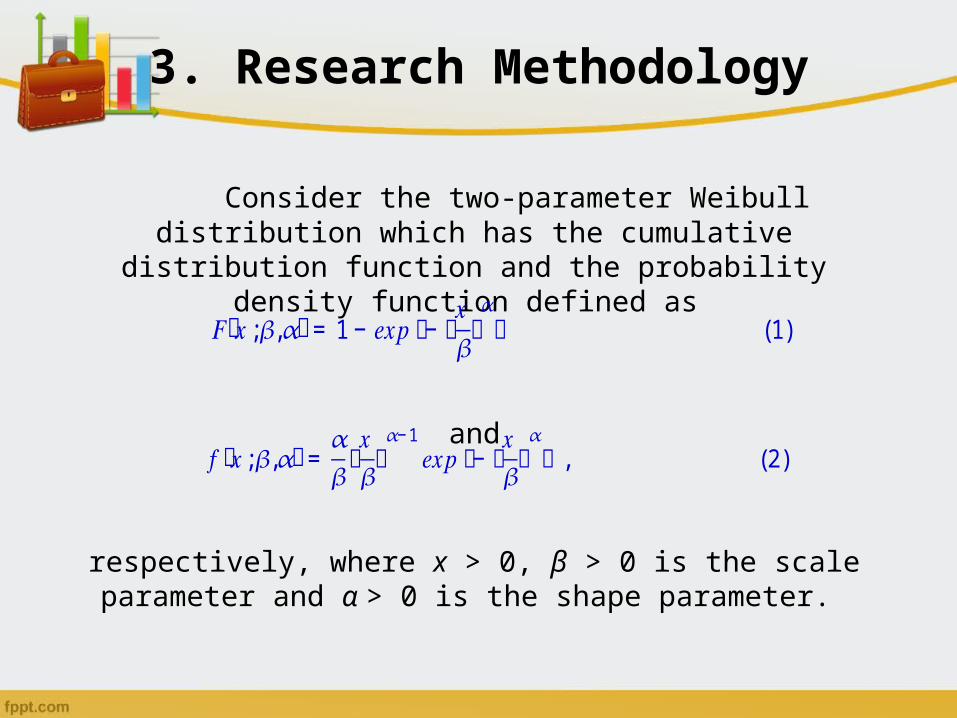
Consider the two-parameter Weibull distribution which has the cumulative distribution function and the

probability density function defined as

and

respectively, where x > 0, β > 0 is the scale parameter and α > 0 is the shape parameter.

𝐹ሺ𝑥;𝛽,𝛼ሻ= 1− 𝑒𝑥𝑝−൬𝑥𝛽൰𝛼

൨ (1)

𝑓ሺ𝑥;𝛽,𝛼ሻ= 𝛼𝛽൬𝑥𝛽൰𝛼−1 𝑒𝑥𝑝−൬𝑥𝛽൰𝛼

൨ , (2)

3. Research Methodology

Empirical Likelihood Method

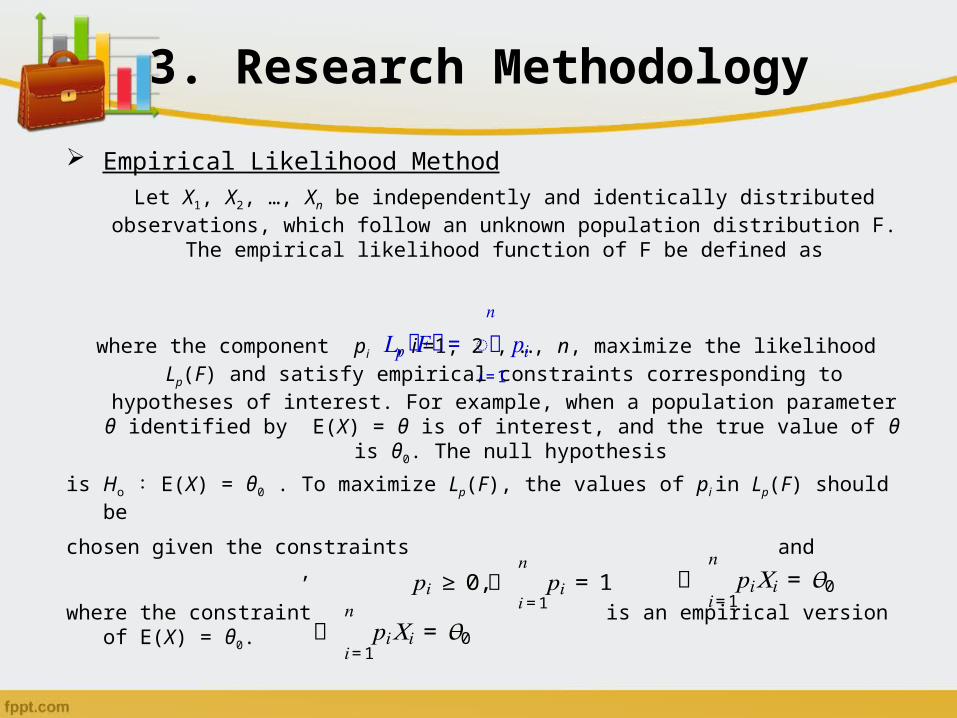
Let X1, X2, …, Xn be independently and identically distributed observations, which follow an unknown population distribution F. The

empirical likelihood function of F be defined as

where the component pi , i =1, 2 , …, n, maximize the likelihood Lp(F) and satisfy empirical constraints corresponding to hypotheses of interest. For example, when a population parameter θ identified by E(X) = θ is

of interest, and the true value of θ is θ0. The null hypothesis

is Ho ∶ E(X) = θ0 . To maximize Lp(F), the values of pi in Lp(F) should be

chosen given the constraints and ,

where the constraint is an empirical version of E(X) = θ0.

𝐿𝑝ሺ𝐹ሻ= ෑ� 𝑝𝑖𝑛

𝑖=1

𝑝𝑖 ≥ 0, 𝑝𝑖 = 1𝑛𝑖=1

𝑝𝑖𝑋𝑖 = 𝜃0𝑛𝑖=1

𝑝𝑖𝑋𝑖 = 𝜃0𝑛𝑖=1

3. Research Methodology

Empirical Likelihood Method (cont.)

The empirical log-likelihood ratio statistic to test θ = θ0 is given by

where R(θ) is the empirical log-likelihood ratio function defined through the definition of the empirical likelihood ratio function by Owen (1988).

𝑅ሺ𝜃0ሻ= max൝ log ሺ𝑛𝑝𝑖ሻ ; 𝑝𝑖 ≥ 0,𝑛𝑖=1 𝑝𝑖

𝑛𝑖=1 = 1, 𝑝𝑖𝑥𝑖

𝑛𝑖=1 = 𝜃0ൡ

3. Research Methodology

Goodness-of-Fit Test

The goodness-of-fit test is a statistical test to determine whether the observations are consistent

with the particular statistical model. It describes how well the particular model fits a set of observations.

Measures of goodness of fit typically summarize the discrepancy between observed values and the

values expected under a statistical model.

3. Research Methodology

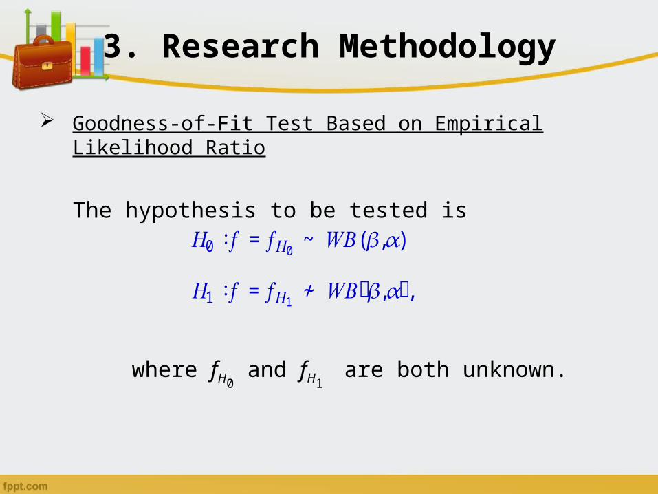
Goodness-of-Fit Test Based on Empirical Likelihood Ratio

The hypothesis to be tested is

where fH0 and fH1

are both unknown.

𝐻0 ∶ 𝑓= 𝑓𝐻0 ~ 𝑊𝐵(𝛽,𝛼)

𝐻1 ∶ 𝑓= 𝑓𝐻1 ≁ 𝑊𝐵ሺ𝛽,𝛼ሻ,

3. Research Methodology

Goodness-of-Fit Test

When density functions fH0 and fH1

are completely

known, the most powerful test statistics is the likelihood ratio

where under the null hypothesis X1, X2, …, Xn follows a Weibull distribution with parameters β and .

𝐿𝑅= ς 𝑓𝐻1𝑛𝑖=1 ሺ𝑋𝑖ሻς 𝑓𝐻0𝑛𝑖=1 ሺ𝑋𝑖ሻ= ς 𝑓𝐻1𝑛𝑖=1 ሺ𝑋𝑖ሻς 𝛼𝛽ቀ𝑥𝑖𝛽ቁ𝛼−1 𝑒𝑥𝑝ቂ−ቀ𝑥𝑖𝛽ቁ𝛼

ቃ𝑛𝑖=1 , (3)

3. Research Methodology

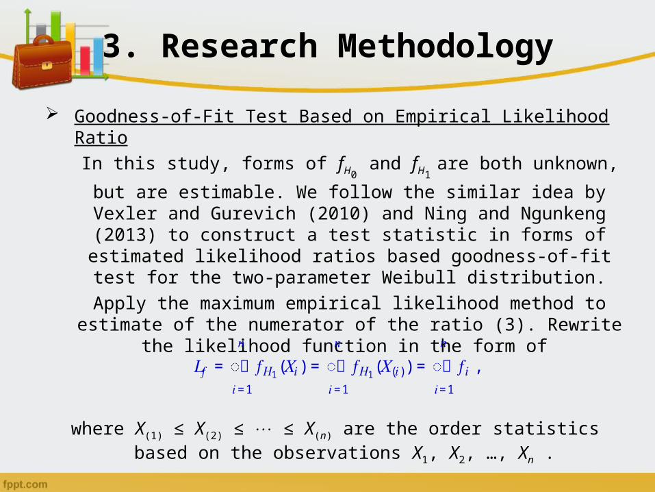
Goodness-of-Fit Test Based on Empirical Likelihood Ratio

In this study, forms of fH0 and fH1

are both unknown, but are

estimable. We follow the similar idea by Vexler and Gurevich (2010) and Ning and Ngunkeng (2013) to construct a test

statistic in forms of estimated likelihood ratios based goodness-of-fit test for the two-parameter Weibull distribution.

Apply the maximum empirical likelihood method to estimate of the numerator of the ratio (3). Rewrite the likelihood

function in the form of

where X(1) ≤ X(2) ≤ ≤ ⋯ X(n) are the order statistics based on the observations X1, X2, …, Xn .

𝐿𝑓 = ෑ� 𝑓𝐻1(𝑋𝑖)𝑛𝑖=1 = ෑ� 𝑓𝐻1(𝑋(𝑖))𝑛

𝑖=1 = ෑ� 𝑓𝑖𝑛

𝑖=1 ,

3. Research Methodology

Goodness-of-Fit Test Based on Empirical Likelihood Ratio

Following the maximum empirical likelihood method, we can derive values of fi that maximize Lf and satisfy the empirical constraints under the alternative hypothesis H1. Obviously, values of fi should

be restricted by the equation ∫ f(s)ds = 1. Thus, we need an empirical form of the constraint ∫ f(s)ds = 1. We first give the following lemma by Vexler and Gurevich (2010) to obtain this empirical constraint.

Lemma 1 Let f(x) be a density function. Then

where X(j-m) = X(1) if j-m ≤ 1 and X(j+m) = X(n) , if j+m ≥ n.

න 𝑓ሺ𝑥ሻ𝑑𝑥𝑋(𝑗+𝑚)

𝑋(𝑗−𝑚)𝑛

𝑗=1 = 2𝑚 න 𝑓ሺ𝑥ሻ𝑑𝑥𝑋(𝑛)

𝑋(1)− (𝑚−𝑘)𝑚−1

𝑘=1 න 𝑓ሺ𝑥ሻ𝑑𝑥𝑋(𝑛−𝑘+1)

𝑋(𝑛−𝑘)− (𝑚−𝑘)𝑚−1

𝑘=1 න 𝑓ሺ𝑥ሻ𝑑𝑥𝑋(𝑘+1)

𝑋(𝑘)

≅ 2𝑚 න 𝑓ሺ𝑥ሻ𝑑𝑥𝑋(𝑛)

𝑋(1)− 𝑚(𝑚− 1)𝑛 (3)

3. Research Methodology

Goodness-of-Fit Test Based on Empirical Likelihood Ratio

It is obvious that since and we denote

, using the empirical approximation to the

remainder term in Lemma 1, we have

From Lemma 1,we can empirically estimate δm via

Notice that δm → 1 when m ⁄ n → 0 as m, n→∞.

න 𝑓ሺ𝑥ሻ𝑑𝑥𝑋(𝑛)𝑋(1) ≤ න 𝑓ሺ𝑥ሻ𝑑𝑥∞

−∞ = 1

𝛿𝑚 = 12𝑚 න 𝑓ሺ𝑥ሻ𝑑𝑥≤ 1𝑋(𝑗+𝑚)

𝑋(𝑗−𝑚)𝑛

𝑗=1

𝛿𝑚 ≅ න 𝑓ሺ𝑥ሻ𝑑𝑥𝑋ሺ𝑛ሻ

𝑋ሺ1ሻ−ሺ𝑚− 1ሻ2𝑛 ≤ 1−ሺ𝑚− 1ሻ2𝑛 .

𝛿መ𝑚 = න 𝑑𝑥𝐹𝑛൫𝑋ሺ𝑛ሻ൯𝐹𝑛൫𝑋ሺ1ሻ൯

−ሺ𝑚− 1ሻ2𝑛 = 1− 1𝑛−ሺ𝑚− 1ሻ2𝑛 .

3. Research Methodology

Goodness-of-Fit Test Based on Empirical Likelihood Ratio

By applying the mean value theorem to the term of ,

we have

Thus, the empirical constraint under the alternative hypothesis H1 is given by

න 𝑓ሺ𝑥ሻ𝑑𝑥𝑋(𝑗+𝑚)

𝑋(𝑗−𝑚)𝑛

𝑗=1

න 𝑓ሺ𝑥ሻ𝑑𝑥𝑋(𝑗+𝑚)

𝑋(𝑗−𝑚)𝑛

𝑗=1 ≅ (𝑋ሺ𝑗+𝑚ሻ

𝑛𝑗=1 − 𝑋ሺ𝑗−𝑚ሻ)𝑓൫𝑋ሺ𝑗ሻ൯= (𝑋ሺ𝑗+𝑚ሻ

𝑛𝑗=1 − 𝑋ሺ𝑗−𝑚ሻ)𝑓𝑗.

𝛿𝑚 = 12𝑚 න 𝑓ሺ𝑥ሻ𝑑𝑥≅ 12𝑚 (𝑋(𝑗+𝑚)𝑛

𝑗=1 − 𝑋(𝑗−𝑚))𝑓𝑗 ≜ 𝛿መ𝑚 ≤ 1𝑋(𝑗+𝑚)

𝑋(𝑗−𝑚)

𝑛𝑗=1

3. Research Methodology

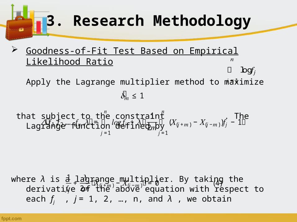
Goodness-of-Fit Test Based on Empirical Likelihood Ratio

Apply the Lagrange multiplier method to maximize

that subject to the constraint . The Lagrange function defined by

where λ is a lagrange multiplier. By taking the derivative of the above equation with respect to each fj , j = 1, 2, …, n, and λ , we obtain

log𝑓𝑗𝑛𝑗=1

𝛿መ𝑚 ≤ 1

𝛬ሺ𝑓1,𝑓2,…,𝑓𝑛,𝜆ሻ= 𝑙𝑜𝑔𝑓𝑗𝑛𝑗=1 + 𝜆ቌ 12𝑚 (𝑋(𝑗+𝑚)

𝑛𝑗=1 − 𝑋(𝑗−𝑚))𝑓𝑗 − 1ቍ

1𝑓𝑗 + 𝜆2𝑚൫𝑋(𝑗+𝑚) − 𝑋(𝑗−𝑚)൯= 0 (4)

3. Research Methodology

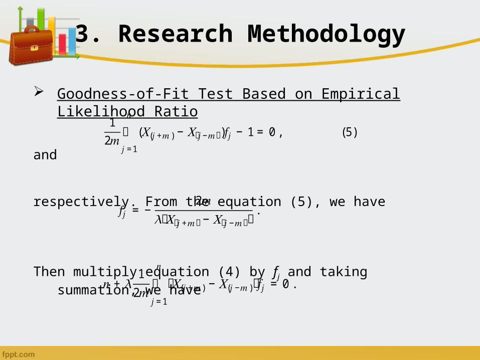
Goodness-of-Fit Test Based on Empirical Likelihood Ratio

and

respectively. From the equation (5), we have

Then multiply equation (4) by fj and taking summation, we have

12𝑚 (𝑋(𝑗+𝑚)𝑛

𝑗=1 − 𝑋ሺ𝑗−𝑚ሻ)𝑓𝑗 − 1 = 0 , (5)

𝑓𝑗 = − 2𝑚𝜆൫𝑋ሺ𝑗+𝑚ሻ− 𝑋ሺ𝑗−𝑚ሻ൯ .

𝑛 + 𝜆 12𝑚 ൫𝑋(𝑗+𝑚) − 𝑋(𝑗−𝑚)൯𝑓𝑗𝑛𝑗=1 = 0 .

3. Research Methodology

Goodness-of-Fit Test Based on Empirical Likelihood Ratio

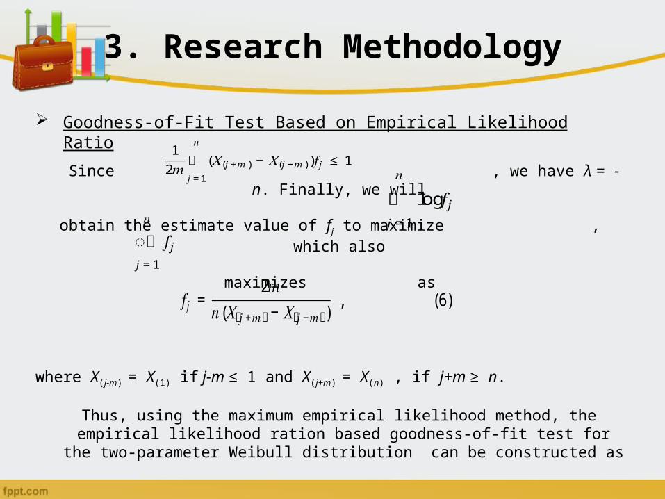
Since , we have λ = -n. Finally, we will

obtain the estimate value of fj to maximize , which also

maximizes as

where X(j-m) = X(1) if j-m ≤ 1 and X(j+m) = X(n) , if j+m ≥ n.

Thus, using the maximum empirical likelihood method, the empirical likelihood ration based goodness-of-fit test for the two-

parameter Weibull distribution can be constructed as

12𝑚 (𝑋(𝑗+𝑚)𝑛

𝑗=1 − 𝑋(𝑗−𝑚))𝑓𝑗 ≤ 1

log𝑓𝑗𝑛𝑗=1

ෑ� 𝑓𝑗𝑛𝑗=1

𝑓𝑗 = 2𝑚𝑛(𝑋ሺ𝑗+𝑚ሻ− 𝑋ሺ𝑗−𝑚ሻ) , (6)

3. Research Methodology

Goodness-of-Fit Test Based on Empirical Likelihood Ratio

where θ = (β, α)' is the parameter vector of a two-parameter Weibull distribution. To maximize the denominator, since the parameters

β and α are unknown, the maximum likelihood estimate of α based on the observations can be applied.

The maximum likelihood estimators and of β and α , respectively, are solutions of the equations:

and

𝑊𝐵𝑛𝑚 = ς 2𝑚𝑛(𝑋ሺ𝑗+𝑚ሻ−𝑋ሺ𝑗−𝑚ሻ)𝑛𝑗=1max𝜽 ς 𝑓𝐻0(𝑋𝑗𝜽)𝑛𝑗=1 (7)

𝛽መ 𝛼ොෑ�

1𝛼ොෑ�+ ln𝑋𝑖𝑛

𝑖=1 − σ 𝑋𝑖𝛼ොෑ�ln𝑋𝑖𝑛𝑖=1σ 𝑋𝑖𝛼ොෑ�𝑛𝑖=1 = 0 𝛽መ= ൭ 𝑋𝑖𝛼ොෑ�𝑛

𝑖=1 ൱

1 𝛼ොෑ�Τ

3. Research Methodology

Goodness-of-Fit Test Based on Empirical Likelihood Ratio

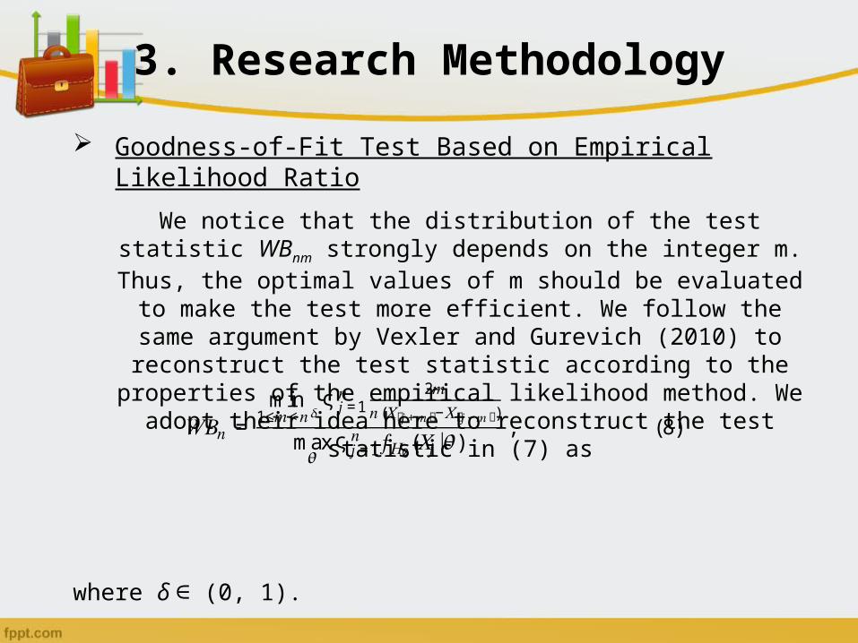
We notice that the distribution of the test statistic WBnm strongly depends on the integer m. Thus, the optimal values of m should be evaluated to make the test more efficient. We follow the same argument by Vexler and Gurevich (2010) to reconstruct the test statistic according to the properties of the empirical likelihood

method. We adopt their idea here to reconstruct the test statistic in (7) as

where δ (0, 1). ∈

𝑊𝐵𝑛 = min1≤𝑚<𝑛𝛿 ς 2𝑚𝑛(𝑋ሺ𝑗+𝑚ሻ−𝑋ሺ𝑗−𝑚ሻ)𝑛𝑗=1max𝜽 ς 𝑓𝐻0(𝑋𝑗𝜽)𝑛𝑗=1 , (8)

3. Research Methodology

Goodness-of-Fit Test Based on Empirical Likelihood Ratio

Similar to the argument of Vexler et al. (2011) and Ning and

Ngunkeng (2013), we take δ =0.5 in the equation (8). Thus, the

final form of the test statistic is

𝑊𝐵𝑛 = min1≤𝑚<ξ𝑛ς 2𝑚𝑛(𝑋ሺ𝑗+𝑚ሻ−𝑋ሺ𝑗−𝑚ሻ)𝑛𝑗=1max𝜽 ς 𝑓𝐻0(𝑋𝑗𝜽)𝑛𝑗=1 (9)

3. Research Methodology

Asymptotic Properties of the Proposed Test Statistic

Denote and

We assume the following conditions hold:

(C1)

(C2) Under the null hypothesis, in probability.

(C3) Under alternative hypothesis, in probability where θ0

is a constant vector with finite components.

(C4) There are open intervals and containing θ and θ0 respectively. There also exists a function s(x) such that

for all x ∈ R and .

ℎ𝑖ሺ𝑥,𝜽ሻ= 𝜕𝑙𝑜𝑔𝑓𝐻0(𝑥;𝜽)𝜕𝜽𝑖 ,𝑖 = 1,2 , 𝜽= ሺ𝜃1,𝜃2ሻ= (𝛽,𝛼)

𝐸(log𝑓ሺ𝑋1ሻ)2 < ∞

𝜽 − 𝜽= max1≤i≤2𝜃𝑖 − 𝜃𝑖→0

𝜽 →𝜽0

0𝑅3 1𝑅3

ℎ(𝑥,)≤ 𝑠(𝑥) ∈0 ∪1

3. Research Methodology

Asymptotic Properties of the Proposed Test Statistic (cont.)

Proposition 1 Assume that the condition (C1)–(C4) hold. Then, under H0,

in probability as →𝑛 ∞,

while, under H1 ,

in probability as →𝑛 ∞.Given condition (C1)–(C4), Proposition 1 shows that the power of the

test goes to 1 as →𝑛 ∞ under the alternative hypothesis. Thus, the proposed test is consistent.

1𝑛logሺ𝑊𝐵𝑛ሻ→0 1𝑛logሺ𝑊𝐵𝑛ሻ→𝐸𝑙𝑜𝑔ቆ 𝑓𝐻1(𝑋1)𝑓𝐻0(𝑋1;𝜃0)ቇ

3. Research Methodology

Calculation of Critical Values and Evaluation of Type I Error Control

To calculate the critical values for fixed sample sizes n = 10, 20, 30, 40, 50, 100, 200, 500, we simulate 5,000

samples from WB(β, ) with different values of (β, ) = (1, 0.5), (1, 2), (1, 4), (1, 8). For each simulated sample, we use R package MASS to estimate parameters β and . Then we can calculate a statistic for each sample

based on equation (9). After we obtain all 5,000 test statistics, we order them and choose 90th, 95th and 99th

percentiles to be the critical values corresponding to the significance level = 0.1, 0.05 and 0.01, respectively.

3. Research Methodology

Calculation of Critical Values and Evaluation of Type I Error Control (cont.)

Consequently, to investigate the performance of the proposed test in controlling the Type I error with the significance level = 0.1, 0.05 and 0.01, we conduct

simulations 5,000 times under WB(β, ) with different values of (β, ) = (1, 0.5), (1, 2), (1, 4), (1, 8)

and sample sizes n = 20, 50, 100, 200, 500, 1000. For each sample, we calculate a sample statistic based on

equation (9) and compares to the critical value. The percentage of rejecting the null hypothesis will be the

size of the proposed test.

3. Research Methodology

Evaluation of the Power of the Proposed Test

In order to study the power of the proposed test, we simulate 10,000 samples with sample size sizes n = 20, 50, 100, 200, 500, 1000 from Beta(0.25, 0.25), Beta(2, 2), N(0,

1) TruncN(-1,1). Then we compute the powers of Kolmogorov-Smirnov test, Cramér-von Mises test,

Anderson-Darling test and the proposed test WBn at the nominal level 0.05.