an empirical estimation of exchange rate determination … · an empirical estimation of exchange...

International Journal of Scientific & Engineering Research Volume 3, Issue 10, October-2012 1

ISSN 2229-5518

IJSER © 2012

http://www.ijser.org

AN EMPIRICAL ESTIMATION OF EXCHANGE RATE DETERMINATION IN INDIA : SINCE 1980-2011

AMANDEEP KAUR

RESEARCH SCHOLAR IN

KURUKSHETRA UNIVERSITY KURUKSHETRA

Abstract— The Historical perspective of foreign exchange Rate determination in India concludes that the Par value system of Exchange

Rate was fixed at 4.15 grains in terms of gold with the pound sterling as the intervention- currency under the time period 1947-1971 in

India. In 1998 foreign exchange management ACT (FEMA) was enacted which takes into account improved economic liberalization and

improved foreign exchange Reserve position during the period (1980-2011). Indian exchange Rate policy has seen a “gradual shift” from a

par value system to basket-peg exchange rate system; and further to a managed floating exchange rate system in India.The study reveals

that a stable exchange Rate may be maintained in the market. For this situation Necessary for the macro economic stability of the

economy. The experience in foreign exchange management in the post reforms years the policy of maintain the flexibility of the exchange

Rate in avoidance with market forces of Demand and Supply without undue volatility as adopted by the RBI, has stood the test of time in

case of India.Exchange Rate Management policy of the RBI supported with sterilization Intervention in the face of Heavy capital inflows in

the recent year also considerably served to the bias in current account besides limiting undue volatility in the exchange Rate.For ensuring

Economic Stability, we have to remove the temporary shocks, increase capital mobility and control the Inflation in the economy. The

exchange Rate Policy should also facilitate the convertibility of Rupee in the Market. Any economic enterprise or person should be able to

convert their holdings of Rupee into any foreign currenciesThe result arrived with the help of annual data present a clear picture of

Exchange Rate determination in India under the period of the study. This implies that PPP theory in India in the long run.

.

—————————— ——————————

1 INTRODUCTION

n the era of globalization and financial liberalization; ex-change Rate (s) play an important role in International Trade and finance. Foreign trade helps the economy to get

through exports the much needed foreign exchange for the development. International Trade as well as the movements of capital Inflows / out flows among different countries necessi-tate the conversion of currencies at an existing exchange Rate. Every nation has its own currency. The currency of India is Rupee (`); USA ($). Most of the international financial transactions involve an exchange rate for one currency into another currency. There may be one or more than one curren-cy involved in the process of exchange, the price of one cur-rency in term of another is known as exchange rate. Exchange Rate is the single most, vital relative price in the financial world. In a more open economy, monetary transmission operates through exchange rate effects on net exports and Interest rates that affect the financial portfolio.In the International finance literature, various theoretical models are available to analyze the exchange rate behaviour. While the exchange rate model existed period to 1970s (Nurkse, 1944; Mundell, 1961, 1962,1963);the most of them were based on the fixed price assumption, with the advent of the floating ex-change rate regime amongst major Industrialized countries in the early 1970s. India's exchange rate policy has been evolved over time in line with the gradual opening up of economy as a part of the broader strategy of macro economic reforms and liberal-ization since the early 1990. In the post independence period, India's exchange Rate system the rupee was linked with

pound sterling. In order to overcome the weaknesses associ-ated with a single currency peg and to ensure stability of the exchange Rate, the rupee w.e.f. September 1975 was pegged to a basket of currencies till the early 1990s. The exchange rate regime in India can best be charac-terized as Intermediate between fully managed and 20th cen-tury faced a severe macroeconomic crisis in India. Indian economy faced the problem of exchange rate which was gross-ly overvalued and the rupee was devalued by about 18 per-cent in two stages in July 1991. At the same time, the govern-ment has introduced the Liberalized Exchange Rate Manage-ment System (LERMS); and thereby ending an era in dual ex-change rate regime. This system was abolished in March 1993. The dual exchange rate was replace by a unified external rate system in March 1993. Since then the external value of the In-dian rupee has been determined by Market forces. The Rupee attained current account convertibility in August 1994. The exchange rate policy in recent years has been guided by the broad principles with flexibility, without a fixed or a pre announced target or a band while allowing the underlying demand and supply conditions to determine the exchange rate movements over a period. In the year 2006-07, the average annual exchange rate of rupee was 45.25 per US $ and Rs. 58.64 per pound sterling. During the fiscal year 2007-08 due to high capital inflows, the rupee appreciated against major international currencies. The appreciation was 12.4 percent against the US $. During 2009-2010; the rupee depreciated against ma-jor International currencies except pound sterling due to de-

I


ISSN 2229-5518

IJSER © 2012


celeration in capital flows and trade deficit. Exchange Rate is the Single Most vital relative Price in the financial World. In an open economy, Monetary trans-mission operates through exchange- Rate effect by a number of economic variables such as: exports, Imports, Balance of trade, foreign exchange Reserves, Gold, SDR's Money Supply (M1,M2, M3, M4), Reserve Money, wholesale Price Index (WPI) consumer Price Index (CPI), Balance of Payment, NEER, REER. Empirical Studies applying various model of ex-change Rate determination on a country by county basis over the modern exchange rate period have been of enormous Im-portance in formulating appropriate exchange Rate Policy Since they can provide useful Information about exchange Rate market Behaviour. The main objective of this research paper is to study the factors that determine the exchange rate in the India. In this paper, we apply the common theory and Model of the PPP and Monetary Models. Thus, essentially this paper is structural to test foreign exchange Rate determination Model for India by Appling econometric Models. The research paper has been divided into five Sec-tions. The first Section discuses the SURVEY OF LITERA-TURE for foreign Exchange Rate determination and second section discuses the Historical Perspective of Foreign Ex-change Rate In India. Section - III analyze the methodology and econometric analysis; and also use the Technique of unit Root test for stationarity and also used the OLS Meth-od.section-iv explain the empirical estimation of foreign ex-change rate determination since-1980-2011 Section - V deals with the Main conclusion and policy implication of this chap-ter.

SECTION-1 SURVEY OF LITERATURE

Recent years, particularly in the context of globalization and currency crises have seen a main issues relating to the exchange rate regime. Which is evident in large and growing body of theoretical and empirical literature on exchange rate determination. The review of literature in the context of de-veloping countries is related by and large to the empirical body of research devoted to testing the applicability of the purchasing power parity [PPP] concept for exchange rate de-termination. Recently the literature on foreign exchange rate determination emphasized a monetarist approach with most of its versions assuming strict [PPP].Many theoretical and em-pirical studies have been undertaken to assess the foreign ex-change rate determination.

Before exploring new phenomena, it is necessary to look in-to various aspects already studied. As research is a continuous process and it must have some continuity with earlier facts. The knowledge gathered in the past should be consolidated to keep it on record for future use. It is like consulting attempts to present a review of some of the important research findings relevant to the objective of present study.

Craig S. Hakkio (1981);In his study examines the conven-tional monetary equation of exchange rate determination. un-der certain erogeneity conditions, one can write the price level.

At home and abroad as the ratio of the nominal money supply to the demand for real money balances. He estimate the ex-change rate as a function of the money supply differential, income differential, and interest rate differential.

Krueger, Anne(1983);In his study examines exchange rate determination as it emerged in the decade of the 1970s. the theory of exchange rate determination is based upon an ana-lytical structure equivalent to that analyzing the determinants of the balance of payment under fixed exchange rate. The dif-ference is that the shifts in excess demand for foreign ex-change lead to quantity adjustments under fixed rate and price adjustments under flexible rates.

Mitsuhiro Fukao (1983);in his paper explain the Interna-tional transaction have increasingly been denominated in oth-er currencies such as the German mark, the Japanese yen ,and Swiss franc .When Japan intervenes in the foreign exchange market by selling dollars and buying yen this affect the dollar-mark, exchange rate.

Williamson (1994) In his study particularly in the context of EU member states in transition, in his approach that takes into account variables such as unemployment and inflation as de-terminants of exchange rate equilibrium.

R.N. Aggarwal (2000);In his study has been done 1971-1972 to 1996-1997 time period. The variable is used in their study is prices, interest rates, and money supply in the home and for-eign country are found to explain the behaviour of the bilat-eral exchange rate. Other significant variable found are bal-ance of payment and foreign exchange reserves. The result show that the model can be used for forecasting the exchange rate in the short run.

Mohammad Najand and Charlotte Bond (2000);In his study compares the forecasting accuracy of state space techniques based on the monetary models of exchange rate with univari-ate and random walk models for four countries. A state space vector that contains variables based on the monetary model easily outperforms.

Renu Kohli (2000);In her study mainly used 1993-1999 time period. The change in regime in India from a multi-currency peg to a floating price convertibility provides sufficient moti-vation for a preliminary analysis of the country’s exchange rate behaviour and management between 1993-1999. using international experience with floating exchange rate as a refer-ence point, their paper examines these changes in a compara-tive perspective. Result is the response of the central bank to exchange rate instability during this period.

Sweta Chaman Saxena [2001];In her paper examines the links between India’s exchange rate, trade flows and the trade regime. Her paper estimates some standard trade elasticities before and after the commencement of reform to examine the effects of this structural change.

Sitikantha Pattanaik, Arghya Kusum Mitra [2001];In his study show that in India, besides foreign exchange market interventions and use of several administrative measures RBI has occasionally resorted to the high rate of interest option during major episodes of significant pressures on the external value of the rupee. An empirical assessment suggests that one standard deviation shock to the call rate leads to rupee appre-ciation in the very second month. Similarly for one standard


ISSN 2229-5518

IJSER © 2012


deviation shock to net interventions, the exchange rate appre-ciates gradually by a few paise over five months.

Lin Jun-Qing, Huang Zuhui And Zhan Ming-Hua [2002];His model shows that central banks can adjust ex-change rate by several policy instruments and that different instruments may have different effects on exchange rate de-termination. He specifies potential policy instruments for cen-tral bank as well as their policy effects.

Renu Kohli (2002);In her paper tests for mean-reversion in real exchange rate for India during the recent float period. She find evidence of mean- reversion in real exchange rate series constructed with the consumer price index as deflator, as well as for a series constructed using the ratio of wholesale and consumer price indexes to proxy for shares of tradable and non-tradable goods.

P.R. Bhatt (2002); In his study was empirically investigated between 1970 and 1998 –which covers the oil boom of the 1970s, the collapse of the oil market prices in the early 1980s and the structural adjustment programme of 1986.In his study examines the portfolio composition of commercial bank and its impact on the economy. Their result of the analysis suggest that portfolio variables –loans and investment contribute sig-nificantly to our cross national product for the period under review.

Ozlale and Yeldan (2002) ;Developed a state space model to estimate the equilibrium exchange rate using exchange rate volatility short term capital movements, industrial production, inflation budget balance of public sector, openness and lags of explanatory variables. In efforts made since the mid- 1990s, many studies have also been employing micro founded gen-eral equilibrium open economy models for determination of real exchange rate.

Hyun-Jae Rhee (2002); In his study the role of psychological impact is examined by investigating the determination of ex-change rate, especially the U.S dollar. He has been applied to the Korean economic crisis which occurred between January 1997 and June 1999.

Golaka C.Nath and G.P. Samanta (2003);In their study ex-amines the causal relationship between returns in stock mar-ket and foreign exchange market in India. Using daily data in the study from March 1993 to December 2002, they found that causal link is generally absent; though in recent years their has been strong causal influence from stock market return to for-eign exchange market return. The results however; are tenta-tive and a need further in-depth research to identify the causes and consequences of the findings.

K.Sham Bhat And R. Rajendran (2003);Their study investi-gated the empirical validity of the monetary model of ex-change rate determination for Indian rupee, pound sterling and yen in terms of U.S dollar. The necessary monthly infor-mation were collected from the international financial statis-tics for the year 1975:10 to 1998:05. The model proves that the exchange rate are not determined by purely monetary factors. The study provides scope for developing a comprehensive structural model by incorporating other fundamental varia-bles like trade balance, reserve position, government’s fiscal deficit as percentage to GDP, public debt position etc. to judge the value and direction of exchange rate movements.

R.K. Pattnaik, Muneesh Kapur, S.C. Dhal (2003);Their study present the Indian experience of exchange rate management against the backdrop of international developments both at the theoretical and empirical levels. In Indian experience the last five decades since independence the exchange rate regime in India has transited from a per value system of the IMF dur-ing the 1950 and the 1960 to a basket-peg during the 1970 to 1980 and eventually culminating in the present from of a mar-ket determined exchange rate regime since march 1993 via a transitional phase of a dual exchange rate between march 1992—February 1993. the empirical exercise undertaken indi-cates that monetary policy has been successful in ensuring orderly condition in the foreign exchange market and contain-ing the impact of exchange rate pass-through effect on domes-tic inflation. Real shocks are predominantly responsible for movements in real as well as nominal exchange rate.

Santi Chaisrisawatsuk and Subhash C.Sharma (2004); In their paper examine the long run equilibrium relationship be-tween exchange rate and currency substitution for a number of countries i.e. Indonesia ,Japan, Korea, Malaysia, Singapore and Thailand for the period 1980-1996. The hybrid portfolio-monetary model of exchange rate determination is derived and extended to incorporate the currency substitution factor and this is objective of the study. The evidence supporting a profound impact of currency substitution in determining long run exchange rates for Indonesia, Malaysia, Singapore and Thailand. Therefore, for these countries, the issue of currency substitution is worth a consideration as they are recently adopting the flexible exchange rate system.26

Mohsin Khan (2004); Investigated the applicability of the

Balassa- Samuelson Effect on the long-run behaviour of real exchange rates in developing countries based on a panel data sample of 16 developing countries. The empirical evidence obtained underscored the significance of the traded-non-traded productivity differential in determining the relative price of non-traded goods, and hence the relative price ratio which in tern exerted a significant effect on the real exchange rate thereby providing a robust verification of Balassa-Samuelson effects for developing countries.27

Chai-On Lee (2005); In his paper presents a theory that the value of foreign moneys are not determined on the exchange markets but outside of them. 1. Even fiat money has a com-modity character within the circle of commodity producers in the least to which any monetary and/or banking institute can-not belong.

Its three figures are to show symmetry between the struc-ture of the dual exchange rate and that of the dual price of gold.

Bohn, Frank (2006) ;In his paper offers a theoretical explanation for the determination of exchange rates under specific conditions which could be found in some OECD and newly industrialized countries in an obstfeld (1994) frame-work extended to incorporate government expropriation re-neging on a fixed exchange rate promise unambiguously pro-duces short term benefits but long term losses.

Himanshu Joshi (2007);In his paper attempts an estimation of the real equilibrium exchange rate for India for the period


ISSN 2229-5518

IJSER © 2012


in the latter half of the 1990s. The period of study is 1996: Q1 to 2005: Q4 quarterly. the model identifies the permanent im-pact of three fundamental structural shocks, viz real demand, supply and nominal shocks. The empirical result finding that the variability in the real exchange rate in India is explained predominantly by permanent real demand shocks followed by nominal and supply shocks. The significance of real demand shocks underpin the important of efforts of the RBI aimed at sterilizing capital inflows and maintaining stable conditions in the foreign exchange market. Since the aggregate nominal shocks explain just about 30% of the forecast error.

Christian Dreger, Georg Stadtmann (2007); In their paper, we use a unique disaggregated data set to model the expecta-tions of the yen/USD exchange rate of about 50 leading for-eign exchange rate professional. The survey includes not only exchange rate projections but also expectations regarding macroeconomic fundamentals, like GDP growth, inflation, interest rate. The result is heterogeneity in exchange rate in the expectation of macroeconomic fundamentals is not sufficient to explain the heterogeneity in exchange rate expectations.

Mita H.Suthar (2008); in his study is used 1996 to 2007 time period for the purpose. The present research tests validity of this hypothesis in association with the exchange rate determi-nation between the Indian rupee and the US dollar. He ob-served that the monetary policy intentions depicted by the bank rate of the RBI, the short run and long term domestic interest differentials and interest yield differentials and the rate of change of foreign exchange reserves have a significant impact on the monthly average of the exchange rate between Indian rupee and the US dollar and quite in line with the eco-nomic theory.

Martin D.D.Evans and Richard K.Lyons (2008); In their pa-per addresses whether transaction flow in foreign exchange market convey information about fundamentals..

MD. Nisar Ahmed Shams (2008); In his paper presents find-ings on the long-run purchasing power parity (PPP) in Bang-ladesh economy during the period 1971/1972- 2005/2006. The result is deviations in domestic and foreign prices are not re-flected in nominal exchange rate changes. Therefore PPP theo-ry should be considered as a short-cut rather than an alterna-tive in finding a complete model of exchange rate determina-tion.

Jeevan Kumar Khundrakpam (2008);in his paper examines the behaviour of exchange rate pass-through to domestic pric-es in India after the reforms initiated in the early 1990s.unlike observed in several countries, he finds a rise in exchange rate pass-through to domestic prices until recent years. Besides economic factors typically associated with economic liberaliza-tion, the persistence of higher inflation is an important factor for the rise in pass-through.

C.Veeramani (2008); In his articles explores the relationship between the real effective exchange rate and exports for the period 1960-2007 using world trade organization and reserve bank of India data, He finds that the appreciation of the REER leads to a fall in the dollar value of India’s merchandise ex-ports. It also forecasts the growth of merchandise export over the medium term.

SECTION-11

Historical Perspective of Foreign Exchange Rate In India The exchange rate regime in India can best be characterized

as Intermediate between fully managed and freely – floating regimes. Exchange rate policy is generally viewed as sub serv-ing the monetary policy stance.

It is now common knowledge that: (1) India in the last decade of twentieth century faced a

severe macroeconomic crisis. (2) One of the problems facing the Indian economy was

that the exchange rate was grossly overvalued. The rupee was historically linked pegged to the pound ster-

ling. Earlier during British regime and till late Sixties, most of India's trade transactions were dominated to pound sterling. Under Bretton Woods System – as a member of IMF Indian declared its per value of rupee in terms of gold. In the post independence period, India’s exchange rate policy has seen a shift from a par value system to a basket-peg and further to a managed float exchange rate system. During the period 1947 till 1971, India followed the par value system of the exchange rate whereby the rupee’s external par value was fixed at 4.15 grains of fine gold. The RBI maintained the par value of the rupee within the permitted margin of ±1% using pound ster-ling as the intervention currency. The devaluation of the rupee in September 1949 and June 1966 in terms of gold resulted in the reduction of the par value of rupee in terms of gold to 2.88 and 1.83 grains of fine gold, respectively. Since 1966, the ex-change rate of the rupee remained constant till 1971

After Smithsonian Agreement in Dec. 1971, The Rupee was de-linked from US $ and again link to pound sterling. This parity was maintained with a band of 2.25%. Due to poor fun-damental pound got depreciated by 20%, which cause rupee to depreciate.

, the rupee also remained stable against dollar. In order to overcome the weaknesses associated with a single currency peg and to ensure stability of the exchange rate, the rupee, with effect from September 1975, was pegged to a basket of currencies. The currencies included in the basket as well as their relative weights were kept confidential by the Reserve Bank to discourage speculation.

January 1, 1984 the sterling rate schedule was abolished. The Interest element which was hitherto in Built the exchange rate was also de linked. The Interest was to recovered from the customers separately. This not only allowed transparency in the exchange rate quotation but also was in tune with Interna-tional practice in this regard.

The liquidity crunch in 1990 and 1991 on foreign exchange only hastened the process. In 1992 New system LERM system announced.

By the late ‘eighties and the early ‘nineties, it was recog-nized that both macroeconomic policy and structural factors had contributed to balance of payment difficulties. The current account deficit widened to 3.0 per cent of GDP in 1990-91 and the foreign currency assets depleted to less than a billion dol-lar by July 1991. It was against this backdrop that India em-barked on stabilization and structural reforms to generate im-pulses for growth.

In March 1992 The Rupee was made partially convertible on the current account. Under the dual exchange


ISSN 2229-5518

IJSER © 2012


rate system 40% of the export earning were to be surrendered at the official exchange and for the rest of all 60%

SECTION-111 METHODOLGY AND ECONOMETRIC ANALYSIS The objective of this Section is to present an overview

of some of the most relevant models of real exchange Rate Determination. These Include the unit Root test apply (Ran-dom walk Model), the Purchasing Power Parity model and the Flexible Price Monetary Model. These models in which the following abbreviations are used and briefly discussed below.

In these models: X : Exports M : Imports FXRe : Foreign Exchange Reserve GDS : Gross Domestic Saving GNP(FC) : Gross National Product of Factor Cost NEER : Nominal Effective Exchange Rate REER : Real Effective Exchange Rate RM : Reserve Money GDP (FC) : Gross Domestic Product at factor cost GDCF : Gross Domestic Capital formation NNP (FC) : Net National Product at factor cost M1,M2, M3, M4 : Money Supply Br : bank rate FXR : Foreign exchange Rate MODELS SPECIFICATION OF THE RELEVANT MODELS

ARE DISCUSSED BELOW: 1) MODELS- I

FER = bo+ b1 x + b2M +U …………..(1) 2) MODELS- II

FER = bo+b1 X + U ……………… (2) FER = bo+b1 M + U …………….. (3

3) MODELS - III (High and Positive correlation between all variables and FXR)

FXR: bo+b1x+b2M+b3FXRe+b4M1+b5M2+b6M3 +b7M4+ b8GDS+b9GNP(FC)+b10 Gold + b11NEER6+b12REER6 +b13 RM+b14 GDP(FC) + b15 GDCF +b16 NNP FC +ut ……. (4)

4) MODEL - IV Unit Root SPECIFICATION OF MODEL: VtFxR=Bo+B1Vtx+B2VtM+B3VtBOT+B4VtFXRe+B5VtGold

+B6VtSDRs+B7VtM1+B8VtM2+B9VtM3+B10VtM4+B11VtRM+B12VtWPI+B13VtCPI+B14VtNEER-6+B15VtREER-6+B16VtNEER-36 + B17VtREER-36+B18VtBR. (5)

5) Model- V (PPP) FER = bo+b1 + ut……………. (6) Or

Log FER = bo+b1 (Log P- log p*) +ut ……(7) 6) Model - VI (Flexible Price Monetary Models) 1) (Pt-Pt*) = bo+b1 (mt-mt*) +b2 (yt-yt*) +b3 (it-it*)+ut 2) (Log P- Log P*) = bo+b1 (Lm-Lm*) +b2 (Ly-Ly*) +b3 (Lr-L*r)+ut 3)Log FXR = bo+b1(Lm-Lm*) +b2 (Ly-Ly*) +b3 (Lr-L*r)+ut SECTION- IV AN EMPIRICAL ESITMATION OF FOREIGN EX-

CHANGE RATE DETERMINATION IN INDIA SINCE: 1980-2011.

This Section has been devoted to the Estimation the Foreign

Exchange Rate determination for the period from 1980-2011. The Foreign Exchange rate is a function of exports, imports, balance of payment, WPI, CPI, Foreign Exchange Reserve, SDR'S , Gold, Money supply BOP, NEER, REER, GDP FC , GDS, GDCF. We have used Secondary time series data on the value of Exchange Rate determination; and Macro economic variables are collected from the hand Book of statistics pub-lished by R.B.I

We have also analyzed the impact of economic and monetary variable on foreign exchange Rate determination. The analysis has been made by applying the linear regression equation and unit Root test. The results are presented in table 1.1 to 1.12 in this section.

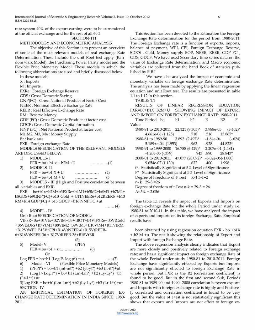
TABLE:-1.1 RESULTS OF LINEAR REGRESSION EQUATION

FXR=B0+B1X+B2M+U SHOWING IMPACT OF EXPORT AND IMPORT ON FOREIGN EXCHANGE RATE: 1980-2011

Time Period bo b1 b2 R R2 F Value

1980-81 to 2010-2011 22.121 (9.305)* 3.988e-05 (3.402)* 4.661e-06 (1.125) .718 .516 13.867*

1980-81 to 1989-90 3.892 (2.497)* -1.84e-04 (-.624) 5.189+e-04 (1.953) .963 .928 44.823*

1990-91 to 1999-2000 16.788 (6.429)* 2.207e-04 (1.481) -4.20e-05 (-.379) .943 .890 28.843* 2000-01 to 2010-2011 47.077 (28.072)* -6.02e-06(-1.800)

9.654e-07 (1.130) .632 .400 1.998 t* - Statistically Significant at 5% Level of Significance F* - Statistically Significant at 5% Level of Significance Degree of Freedom- of F Test K-1 3-1=2 n- k 29-3 =26 Degree of freedom of t Test n-k = 29-3 = 26 At 5% = 2.056 The table 1.1 reveals the impact of Exports and Imports on

foreign exchange Rate for the whole Period under study i.e. 1980-81 to 2010-11. In this table, we have analyzed the impact of exports and imports on its foreign Exchange Rate. Empirical results have

been obtained by using regression equation FXR - bo +b1X

+ b2 M +u. The result showing the relationship of Export and Import with foreign Exchange Rate.

The above regression analysis clearly indicates that Export are more closely and positively related to Foreign exchange rate; and has a significant impact on foreign exchange Rate of the whole Period under study 1980-81 to 2010-2011. Foreign Exchange have significantly effected by Exports but Imports are not significantly effected to foreign Exchange Rate in whole period. But FXR as the R2 (correlation coefficient) is found to be good. But in the first and second Sub, Periods 1980-81 to 1989-90 and 1990- 2000 correlation between exports and Imports with foreign exchange rate is highly and Positive-ly correlated and correlation coefficient is found to be very good. But the value of t test is not statistically significant this shows that exports and Imports are not effect to foreign ex-


ISSN 2229-5518

IJSER © 2012


change Rate. But the overall model of F value is Significant in whole time Period and two sub time period. But in 2000-01 to 2010-11 exports and imports are not significantly affective the foreign Exchange Rate. Exports are negatively related and im-ports are positively related with foreign exchange rate deter-mination TABLE-1.2

RESULTS OF LINEAR REGRESSION EQUATION. FXR= bo + b1X + U SHOWING THE IMPACT OF EXPORT ON FOREIGN EXCHANGE RATE: 1980-2011. Time Period Bo b1 R R2 F Value 1980-81 to 2010-11 21.293 (8.347)* 4.789e-05(5.119)*

.702 .493 26.209* 1980-81 to 1989-90 6.696 (9.502)* 3.865e-04 (7.968)*

.940 .888 63.496* 1990-91 to 1999-2000 17.292 (8.138)* 1.648e-04 (7.943)*

.942 .887 63.093* 2000-01 to 2010-11 47.715 (29.642)* -5.46e-06 (-1.618) .522 .272 2.616 t *- Statistically significant at 5% Level of significance F* - Statistically significant at 5% Level of significance. The table 1.2 We have analyzed the impact of only

exports on foreign exchange Rate. Empirical result have been obtained by using regression equation "FXR = b0+b1X"

The above regression analysis clearly Indicates that exports are more strongly and positively related to foreign exchange rate determination; and has a significant Impact on exchange Rate in whole Period under study 1980-81 to 2010-2011 and also during the Sub- Periods 1980 to 1990 and 1990 to 2000. The value of R2 is very high. Except during the sub period 2010-2011,when the relation between exports and foreign ex-change rate determination is very weak.

TABLE- 1.3 RESULTS OF LINEAR REGRESSION EQUATION FXR

=bo+b1M+U SHOWING THE IMPACT OF IMPORT ON FOREIGN EXCHANGE RATE 1980-2011. Time Period Bo b1 R R2 F Value 1980-81 to 2010-2011 25.081 (9.403)* 1.322e-05 (3.407)*

.548 .301 11.609* 1980-81 to 1989-90 4.730 (6.234)* 3.548e-04 (9.830)*

.961 .924 96.635* 1990-91 to 1999-2000 19.183 (8.726)* 1.203e-04 (6.873)*

.925 .885 47.240* 2000-01 to 2010-2011 44.704 (37.552)* 7.346e-07 (.757)

.275 .076 .573 t *- Statistically significant at 5% Level of significance F* - Statistically significant at 5% Level of significance. The table 1.3 Shows that the import have a positive impact

on Foreign Exchange Rate during whole Period 1980 to 2011 and the sub Period 1980 to 1990 and 1990 to 2000. In this Sub Period, correlation between foreign Exchange Rate and Im-ports is very high. Correlation coefficient (R2) also very high and better goodness of fit. But in the Sub period 2000-2001 to 2010-2011 correlation; and correlation coefficient is very low and also the value of t is not statistically significant.

TABLE- 1.4 MODELS - III - CORRELATION MATRIX ANNUAL DATA - 1980 TO 2011 We have estimated correlation Matrix between exchange

rate and 16 relevant economic variables expected to be linked. The result are presented in table 1.4. Correlation is Significant at the 0.01 level (2.tailed)

High Correlation Matrix Variables Correlation between foreign Exchange Rate

and variable Exports .702** Imports .548**

fx Reserves .633** M1 .747** M2 .748** M3 .729** M4 .732** GDP(FC) .813** GDCF .704** GDS .718** GNP(FC) .514** GOLD .783** Reserve M .749** REER- 6 .910** NEER-6 .849** NNP(FC) .799** **. Correlation is Significant at the 0.01 level (2 tailed) In this table 1.4 show the correlation Matrix between for-

eign exchange rate and all of these variable. The correlation between FXR and all these variable is high and Positive. The table shows that all variables are highly linked with the for-eign Exchange Rate determination.

TABLE-1.5 RESULTS OF LINEAR REGRESSION EQUATION THE IMPACT OF HIGH CORRELATED VAR-

IABLES ON FXR: 1980-2011 Variables bs value t value t value Constant (bo) 5.013 4.776* Export -427e-05 -1.190 Import 4.155e-07 .579 FX R all -4.90e-05 -2.558* M1 -7.32e-05 -1.978 GDP (FC) 4.156e-05 6.580* GDCF -7.21e-05 -2.516* GDS 8.801e-05 -2.239* GNP(FC) -1.56e-07 -.977 GOLD 5.949e-04 3.354* NEER – 6 .324 1.869 REER – 6 -.309 -1.882 Res m -9.87e-06 -.288 M2 40.507 1.201 M3 -3.915 -1.767 M4 -3.636 -1.528 NNP(FC) -4.327 -1.646 R = .997 D.W = 2.264


ISSN 2229-5518

IJSER © 2012


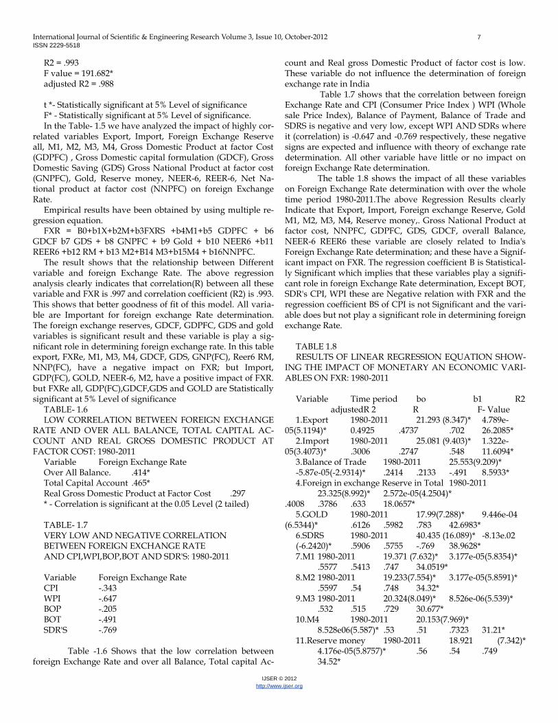
R2 = .993 F value = 191.682* adjusted R2 = .988 t *- Statistically significant at 5% Level of significance F* - Statistically significant at 5% Level of significance. In the Table- 1.5 we have analyzed the impact of highly cor-

related variables Export, Import, Foreign Exchange Reserve all, M1, M2, M3, M4, Gross Domestic Product at factor Cost (GDPFC) , Gross Domestic capital formulation (GDCF), Gross Domestic Saving (GDS) Gross National Product at factor cost (GNPFC), Gold, Reserve money, NEER-6, REER-6, Net Na-tional product at factor cost (NNPFC) on foreign Exchange Rate.

Empirical results have been obtained by using multiple re-gression equation.

FXR = B0+b1X+b2M+b3FXRS +b4M1+b5 GDPFC + b6 GDCF b7 GDS + b8 GNPFC + b9 Gold + b10 NEER6 +b11 REER6 +b12 RM + b13 M2+B14 M3+b15M4 + b16NNPFC.

The result shows that the relationship between Different variable and foreign Exchange Rate. The above regression analysis clearly indicates that correlation(R) between all these variable and FXR is .997 and correlation coefficient (R2) is .993. This shows that better goodness of fit of this model. All varia-ble are Important for foreign exchange Rate determination. The foreign exchange reserves, GDCF, GDPFC, GDS and gold variables is significant result and these variable is play a sig-nificant role in determining foreign exchange rate. In this table export, FXRe, M1, M3, M4, GDCF, GDS, GNP(FC), Reer6 RM, NNP(FC), have a negative impact on FXR; but Import, GDP(FC), GOLD, NEER-6, M2, have a positive impact of FXR. but FXRe all, GDP(FC),GDCF,GDS and GOLD are Statistically significant at 5% Level of significance

TABLE- 1.6 LOW CORRELATION BETWEEN FOREIGN EXCHANGE

RATE AND OVER ALL BALANCE, TOTAL CAPITAL AC-COUNT AND REAL GROSS DOMESTIC PRODUCT AT FACTOR COST: 1980-2011

Variable Foreign Exchange Rate Over All Balance. .414* Total Capital Account .465* Real Gross Domestic Product at Factor Cost .297 * - Correlation is significant at the 0.05 Level (2 tailed) TABLE- 1.7 VERY LOW AND NEGATIVE CORRELATION BETWEEN FOREIGN EXCHANGE RATE AND CPI,WPI,BOP,BOT AND SDR'S: 1980-2011 Variable Foreign Exchange Rate CPI -.343 WPI -.647 BOP -.205 BOT -.491 SDR'S -.769 Table -1.6 Shows that the low correlation between

foreign Exchange Rate and over all Balance, Total capital Ac-

count and Real gross Domestic Product of factor cost is low. These variable do not influence the determination of foreign exchange rate in India

Table 1.7 shows that the correlation between foreign Exchange Rate and CPI (Consumer Price Index ) WPI (Whole sale Price Index), Balance of Payment, Balance of Trade and SDRS is negative and very low, except WPI AND SDRs where it (correlation) is -0.647 and -0.769 respectively, these negative signs are expected and influence with theory of exchange rate determination. All other variable have little or no impact on foreign Exchange Rate determination.

The table 1.8 shows the impact of all these variables on Foreign Exchange Rate determination with over the whole time period 1980-2011.The above Regression Results clearly Indicate that Export, Import, Foreign exchange Reserve, Gold M1, M2, M3, M4, Reserve money,. Gross National Product at factor cost, NNPFC, GDPFC, GDS, GDCF, overall Balance, NEER-6 REER6 these variable are closely related to India's Foreign Exchange Rate determination; and these have a Signif-icant impact on FXR. The regression coefficient B is Statistical-ly Significant which implies that these variables play a signifi-cant role in foreign Exchange Rate determination, Except BOT, SDR's CPI, WPI these are Negative relation with FXR and the regression coefficient BS of CPI is not Significant and the vari-able does but not play a significant role in determining foreign exchange Rate.

TABLE 1.8 RESULTS OF LINEAR REGRESSION EQUATION SHOW-

ING THE IMPACT OF MONETARY AN ECONOMIC VARI-ABLES ON FXR: 1980-2011

Variable Time period bo b1 R2

adjustedR 2 R F- Value 1.Export 1980-2011 21.293 (8.347)* 4.789e-

05(5.1194)* 0.4925 .4737 .702 26.2085* 2.Import 1980-2011 25.081 (9.403)* 1.322e-

05(3.4073)* .3006 .2747 .548 11.6094* 3.Balance of Trade 1980-2011 25.553(9.209)* -5.87e-05(-2.9314)* .2414 .2133 -.491 8.5933* 4.Foreign in exchange Reserve in Total 1980-2011

23.325(8.992)* 2.572e-05(4.2504)* .4008 .3786 .633 18.0657*

5.GOLD 1980-2011 17.99(7.288)* 9.446e-04 (6.5344)* .6126 .5982 .783 42.6983*

6.SDRS 1980-2011 40.435 (16.089)* -8.13e.02 (-6.2420)* .5906 .5755 -.769 38.9628* 7.M1 1980-2011 19.371 (7.632)* 3.177e-05(5.8354)*

.5577 .5413 .747 34.0519* 8.M2 1980-2011 19.233(7.554)* 3.177e-05(5.8591)*

.5597 .54 .748 34.32* 9.M3 1980-2011 20.324(8.049)* 8.526e-06(5.539)*

.532 .515 .729 30.677* 10.M4 1980-2011 20.153(7.969)*

8.528e06(5.587)* .53 .51 .7323 31.21* 11.Reserve money 1980-2011 18.921 (7.342)*

4.176e-05(5.8757)* .56 .54 .749 34.52*


ISSN 2229-5518

IJSER © 2012


12.NNP at factor cost 1980-2011 17.231(7.049)* 9.588e-06(6.89281)* .63 .62 .779 47.51*

13.GDP at factor cost 1980-2011 16.767(7.025)* 8.906e-06(7.2631)* .66 .64 .813 52.75*

14.Gross Domestic Saving 1980-2011 20.365(7.897)* 2.004e-05(5.3654)* .51 .49 .718 28.78*

15.Gross Domestic Capital formulation 1980-2011 20.584(7.839)* 1.896e-05(5.1571)* .49 .47 .704 26.59*

16.WPI 1980-2011 55.100(8.900)* -.118 (-4.41137)* .41 .39 -.647 19.48* 17.CPI 1980-2011 40.932 (6.201)* -2.81e-02 (-1.8991) .11 .08 -.343 3.60 18.Overall balance 1980-2011 26.91(9.743)*

7.416e-05(2.3661)* .17 .14 .414* 5.59*

19.NEER 6- currency 1980-2011 15.975(7.294)* .310(8.339)* .72 .71 .849 69.546*

20.REER 6-curency 1980-2011 14.775(8.533)* .259(11.407)* .82 .822 .910 130.118*

t* – Statistically significant at 5% level of significance F* – Statistically significant at 5% level of significance MODELING PURCHASING POWER PARITY The Purchasing power (PPP) Model asserts that the

exchange Rate between two currencies over any period of time is determined by the change in the two countries Price levels. However an exchange rate in the short run would deviate from PPP mainly due to three disturbances:- actual and ex-pected inflation, Barriers to trade, and shifts in International movements of capital. A fourth factor, the productivity bias occurring when there is relatively faster productivity growth in the tradable sector than in the Non- tradable sector. will also result in a systematic deviation of the Domestic Price.

In the absolute version of PPP, the share of domestic and foreign Prices determines the nominal exchange Rate,

FXR = Where FXR = is the exchange rate Measured as the domes-

tic currency price of a unit of foreign currency. Here P and P* are the domestic and foreign Price level.

By taking logarithms the absolute PPP model is written as: Log FXR = log Pt - log Pt* MONETARY MODEL:- The concept of the Monetary Model of exchange Rate

determination begins with the assumption of ideal capital Mobility. These monetary Model(s) are focused on the "Flexi-ble Price Monetary (FPM).

The Logarithm of the demand for money is assumed to depend on the logarithm of real Income (y) and the loga-rithm of Price level (P) and the level of Nominal Interest rate (r). An identical demand for Money can also be assumed for the foreign country.

TESTING THE PPP AND MONETARY MODELS Annual data are extracted from RBI and International

Financial Statistics (IFS) For a period of 1980 to 2011 with a

total 29 data points. The M2 is used as the proxy for money supply and Income is represented by the real GDP of India and U.S.A. The Bank Rate represent the Interest Rates in India and EURO- Dollar-3 month for Interest Rates in U.S.A. Con-sumer Price Index. (CPI) is used for Price in both country. The exchange rate expressed in rupee per US$ unit. The Time se-ries are first examined for stationarity; and then followed by the Results of the Augmented Dickey- fuller (ADF) test for a single unit Root. The Non- Stationary exchange Rate suggests that a long Run PPP between US $ and (`) Rupee does not ex-ist. If data is not stationary the second order difference must be tested.

TABLE 1.9(A) RESULTS OF UNIT ROOT TEST FOR PPP WITH DICKY

FULLER TEST: 1980-2011 Variables Unit Root Test D.F. Test Bo B1

B2T Durbin Watson Test Conclusion 1) Log FXR I(o) 2) Without trend .105 -5.63e.02(-2.357)

______ 1.518 Non Stationary with Trend .7.586e-02 -2.16e-02(-.277)

-1.20e-03 (-.469) 1.585 Non Stationary I(1) First difference Without trend 1.777e-02 -.675(-3.561)*

_____ 1.917 Stationary with Trend 4.589e-02 -.840 (-3.902)*

-1.48e-03 (-1.498) 1.834 Stationary 3) Log P I(o) Without trend .707 -.281(-1.825) _______ 1.821 Non Stationary with Trend .984 -.353 (-2.212) -5.84e-03 (-1.402) 1.830 Non Stationary I(1) Without trend -1.95e-02 -1.072(-5.377)*

_______ 2.016** Stationary with Trend 2.736e-02 -1.092 (-5.344)* -2.95e-03 (-.631) 2.013** Stationary 3) Log P* I(o) Without trend 7.340e-02 -2.78e-02 (-3.523) *

_______ 1.469 Stationary with Trend .246 -.116(-1.589)

1.187e-03 (1.216) 1.440 Non Stationary I(1) Without trend 8.073e-03 -.656(-3.282)*

__ 1.488 Stationary with Trend 1.484e-02 -.856 (-4.024)* -2.49e-04 (-2.027) 1.510 Stationary * - Indicate the stationery series ** - Indicate the No Autocorrelation Problem Critical Value of Tau Test is 10% (-2.5844), 5% (-2.8951), 1% (-3.5073) Table 1.9 (A) shows that unit Root Test is used for

check the stationarity. In unit Root test, two tests are very use-ful Dickey fuller and augmented Dickey Fuller Test.

Dickey fuller Test Show that all variable are Non- Sta-tionary in level I(0) Series. But in the Integrated level one with I (1) First Difference of time series data of all variable is Sta-tionary But this result show that all variables take Autocorre-


ISSN 2229-5518

IJSER © 2012


lation Problem; for the solution of this problem; we take Augmented Dickey fuller test.

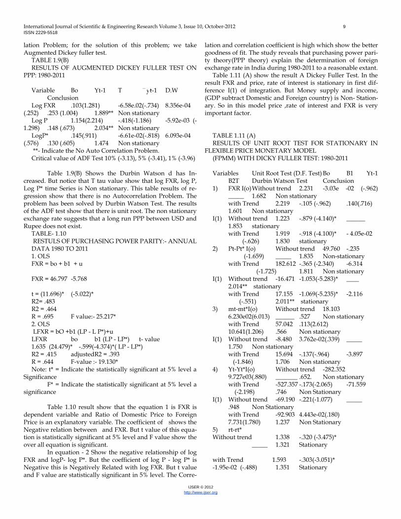
TABLE 1.9(B) RESULTS OF AUGMENTED DICKEY FULLER TEST ON

PPP: 1980-2011 Variable Bo Yt-1 T -1 D.W

Conclusion Log FXR .103(1.281) -6.58e.02(-.734) 8.356e-04

(.252) .253 (1.004) 1.889** Non stationary Log P 1.154(2.214) -.418(-1.186) -5.92e-03 (-

1.298) .148 (.673) 2.034** Non stationary LogP* .145(.911) -6.61e-02(-.818) 6.093e-04

(.576) .130 (.605) 1.474 Non stationary **- Indicate the No Auto Correlation Problem. Critical value of ADF Test 10% (-3.13), 5% (-3.41), 1% (-3.96) Table 1.9(B) Shows the Durbin Watson d has In-

creased. But notice that T tau value show that log FXR, log P, Log P* time Series is Non stationary. This table results of re-gression show that there is no Autocorrelation Problem. The problem has been solved by Durbin Watson Test. The results of the ADF test show that there is unit root. The non stationary exchange rate suggests that a long run PPP between USD and Rupee does not exist.

TABLE- 1.10 RESTULS OF PURCHASING POWER PARITY:- ANNUAL DATA 1980 TO 2011 1. OLS FXR = bo + b1 + u

FXR = 46.797 -5.768

t = (11.696)* (-5.022)* R2= .483 R2 = .464 R = .695 F value:- 25.217* 2. OLS LFXR = bO +b1 (LP - L P*)+u LFXR bo b1 (LP - LP*) t- value 1.635 (24.479)* -.599(-4.374)*( LP - LP*) R2 = .415 adjustedR2 = .393 R = .644 F-value :- 19.130* Note: t* = Indicate the statistically significant at 5% level a

Significance F* = Indicate the statistically significant at 5% level a

significance Table 1.10 result show that the equation 1 is FXR is

dependent variable and Ratio of Domestic Price to Foreign Price is an explanatory variable. The coefficient of shows the Negative relation between and FXR. But t value of this equa-tion is statistically significant at 5% level and F value show the over all equation is significant.

In equation - 2 Show the negative relationship of log FXR and logP- log P*. But the coefficient of log P - log P* is Negative this is Negatively Related with log FXR. But t value and F value are statistically significant in 5% level. The Corre-

lation and correlation coefficient is high which show the better goodness of fit. The study reveals that purchasing power pari-ty theory(PPP theory) explain the determination of foreign exchange rate in India during 1980-2011 to a reasonable extant.

Table 1.11 (A) show the result A Dickey Fuller Test. In the result FXR and price, rate of interest is stationary in first dif-ference I(1) of integration. But Money supply and income, (GDP subtract Domestic and Foreign country) is Non- Station-ary. So in this model price ,rate of interest and FXR is very important factor.

TABLE 1.11 (A) RESULTS OF UNIT ROOT TEST FOR STATIONARY IN

FLEXIBLE PRICE MONETARY MODEL (FPMM) WITH DICKY FULLER TEST: 1980-2011 Variables Unit Root Test (D.F. Test) Bo B1 Yt-1

B2T Durbin Watson Test Conclusion 1) FXR I(o) Without trend 2.231 -3.03e -02 (-.962)

_____ 1.682 Non stationary with Trend 2.219 -.105 (-.962) .140(.716)

1.601 Non stationary I(1) Without trend 1.223 -.879 (-4.140)* ______

1.853 stationary with Trend 1.919 -.918 (-4.100)* - 4.05e-02 (-.626) 1.830 stationary 2) Pt-Pt* I(o) Without trend 49.760 -.235 (-1.659) _____ 1.835 Non-stationary with Trend 182.612 -.365 (-2.340) -6.314 (-1.725) 1.811 Non stationary I(1) Without trend -16.471 -1.053(-5.283)* ____

2.014** stationary with Trend 17.155 -1.069(-5.235)* -2.116 (-.551) 2.011** stationary 3) mt-mt*I(o) Without trend 18.103

6.230e02(6.013) ______ .527 Non stationary with Trend 57.042 .113(2.612)

10.641(1.206) .566 Non stationary I(1) Without trend -8.480 3.762e-02(.339) _____

1.750 Non stationary with Trend 15.694 -.137(-.964) -3.897 (-1.846) 1.706 Non stationary 4) Yt-Yt*I(o) Without trend -282.352

9.727e03(.880) _______ .652. Non stationary with Trend -527.357 -.173(-2.065) -71.559 (-2.198) .746 Non Stationary I(1) Without trend -69.190 -.221(-1.077) _____

.948 Non Stationary with Trend -92.903 4.443e-02(.180)

7.731(1.780) 1.237 Non Stationary 5) rt-rt* Without trend 1.338 -.320 (-3.475)* _____ 1.321 Stationary with Trend 1.593 -.303(-3.051)* -1.95e-02 (-.488) 1.351 Stationary


ISSN 2229-5518

IJSER © 2012


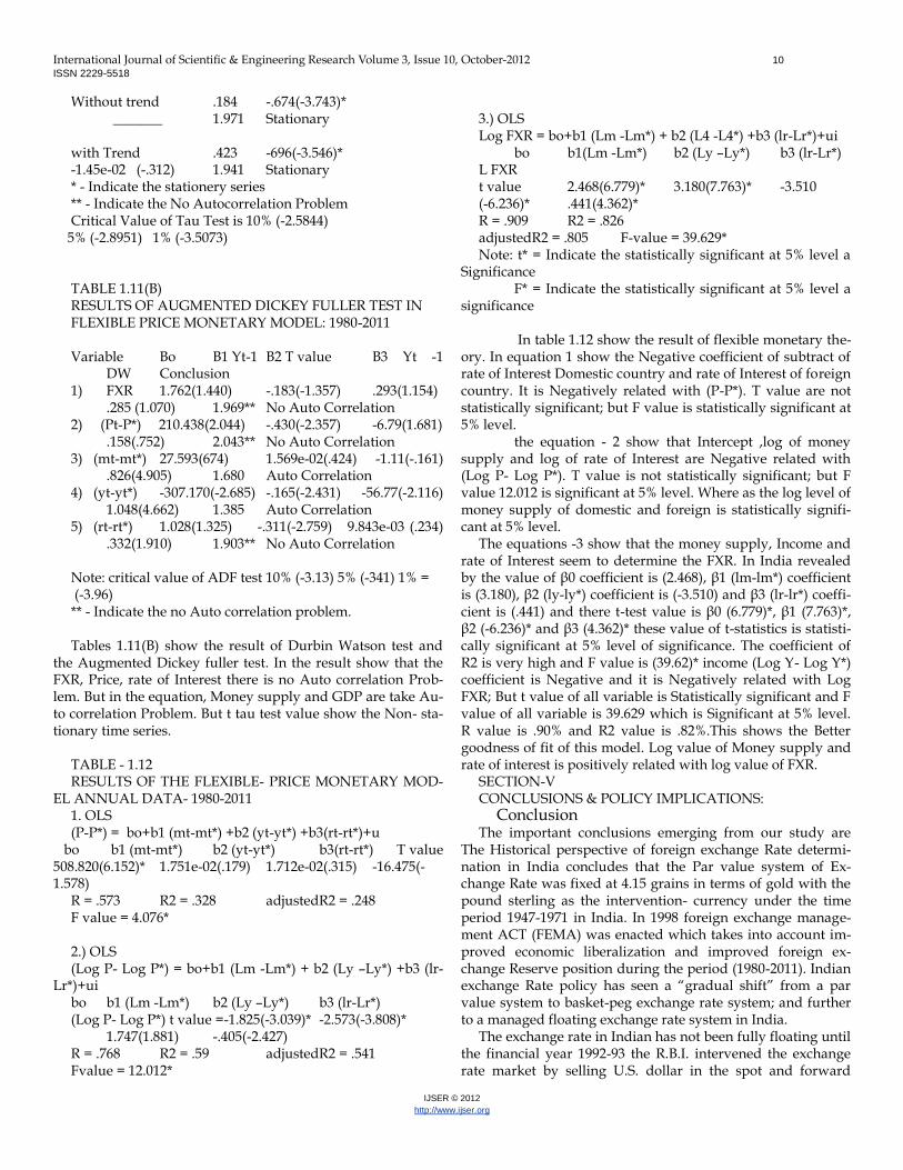
Without trend .184 -.674(-3.743)* _______ 1.971 Stationary with Trend .423 -696(-3.546)* -1.45e-02 (-.312) 1.941 Stationary * - Indicate the stationery series ** - Indicate the No Autocorrelation Problem Critical Value of Tau Test is 10% (-2.5844)

5% (-2.8951) 1% (-3.5073) TABLE 1.11(B) RESULTS OF AUGMENTED DICKEY FULLER TEST IN FLEXIBLE PRICE MONETARY MODEL: 1980-2011 Variable Bo B1 Yt-1 B2 T value B3 Yt -1

DW Conclusion 1) FXR 1.762(1.440) -.183(-1.357) .293(1.154)

.285 (1.070) 1.969** No Auto Correlation 2) (Pt-P*) 210.438(2.044) -.430(-2.357) -6.79(1.681)

.158(.752) 2.043** No Auto Correlation 3) (mt-mt*) 27.593(674) 1.569e-02(.424) -1.11(-.161)

.826(4.905) 1.680 Auto Correlation 4) (yt-yt*) -307.170(-2.685) -.165(-2.431) -56.77(-2.116)

1.048(4.662) 1.385 Auto Correlation 5) (rt-rt*) 1.028(1.325) -.311(-2.759) 9.843e-03 (.234)

.332(1.910) 1.903** No Auto Correlation Note: critical value of ADF test 10% (-3.13) 5% (-341) 1% = (-3.96) ** - Indicate the no Auto correlation problem. Tables 1.11(B) show the result of Durbin Watson test and

the Augmented Dickey fuller test. In the result show that the FXR, Price, rate of Interest there is no Auto correlation Prob-lem. But in the equation, Money supply and GDP are take Au-to correlation Problem. But t tau test value show the Non- sta-tionary time series.

TABLE - 1.12 RESULTS OF THE FLEXIBLE- PRICE MONETARY MOD-

EL ANNUAL DATA- 1980-2011 1. OLS (P-P*) = bo+b1 (mt-mt*) +b2 (yt-yt*) +b3(rt-rt*)+u

bo b1 (mt-mt*) b2 (yt-yt*) b3(rt-rt*) T value 508.820(6.152)* 1.751e-02(.179) 1.712e-02(.315) -16.475(-1.578)

R = .573 R2 = .328 adjustedR2 = .248 F value = 4.076* 2.) OLS (Log P- Log P*) = bo+b1 (Lm -Lm*) + b2 (Ly –Ly*) +b3 (lr-

Lr*)+ui bo b1 (Lm -Lm*) b2 (Ly –Ly*) b3 (lr-Lr*) (Log P- Log P*) t value =-1.825(-3.039)* -2.573(-3.808)*

1.747(1.881) -.405(-2.427) R = .768 R2 = .59 adjustedR2 = .541 Fvalue = 12.012*

3.) OLS Log FXR = bo+b1 (Lm -Lm*) + b2 (L4 -L4*) +b3 (lr-Lr*)+ui bo b1(Lm -Lm*) b2 (Ly –Ly*) b3 (lr-Lr*) L FXR t value 2.468(6.779)* 3.180(7.763)* -3.510 (-6.236)* .441(4.362)* R = .909 R2 = .826 adjustedR2 = .805 F-value = 39.629* Note: t* = Indicate the statistically significant at 5% level a

Significance F* = Indicate the statistically significant at 5% level a

significance In table 1.12 show the result of flexible monetary the-

ory. In equation 1 show the Negative coefficient of subtract of rate of Interest Domestic country and rate of Interest of foreign country. It is Negatively related with (P-P*). T value are not statistically significant; but F value is statistically significant at 5% level.

the equation - 2 show that Intercept ,log of money supply and log of rate of Interest are Negative related with (Log P- Log P*). T value is not statistically significant; but F value 12.012 is significant at 5% level. Where as the log level of money supply of domestic and foreign is statistically signifi-cant at 5% level.

The equations -3 show that the money supply, Income and rate of Interest seem to determine the FXR. In India revealed by the value of β0 coefficient is (2.468), β1 (lm-lm*) coefficient is (3.180), β2 (ly-ly*) coefficient is (-3.510) and β3 (lr-lr*) coeffi-cient is (.441) and there t-test value is β0 (6.779)*, β1 (7.763)*, β2 (-6.236)* and β3 (4.362)* these value of t-statistics is statisti-cally significant at 5% level of significance. The coefficient of R2 is very high and F value is (39.62)* income (Log Y- Log Y*) coefficient is Negative and it is Negatively related with Log FXR; But t value of all variable is Statistically significant and F value of all variable is 39.629 which is Significant at 5% level. R value is .90% and R2 value is .82%.This shows the Better goodness of fit of this model. Log value of Money supply and rate of interest is positively related with log value of FXR.

SECTION-V CONCLUSIONS & POLICY IMPLICATIONS: Conclusion The important conclusions emerging from our study are

The Historical perspective of foreign exchange Rate determi-nation in India concludes that the Par value system of Ex-change Rate was fixed at 4.15 grains in terms of gold with the pound sterling as the intervention- currency under the time period 1947-1971 in India. In 1998 foreign exchange manage-ment ACT (FEMA) was enacted which takes into account im-proved economic liberalization and improved foreign ex-change Reserve position during the period (1980-2011). Indian exchange Rate policy has seen a “gradual shift” from a par value system to basket-peg exchange rate system; and further to a managed floating exchange rate system in India.

The exchange rate in Indian has not been fully floating until the financial year 1992-93 the R.B.I. intervened the exchange rate market by selling U.S. dollar in the spot and forward


ISSN 2229-5518

IJSER © 2012


markets. The results based on six models of estimation show

that all explanatory variables affect the foreign exchange Rate determination Prominent among these variables are: exports, imports, rate of interest, money supply, GDP in the determina-tion of foreign exchange rate.The first model explains the ef-fects of exports and imports on foreign exchange rate during the whole time period 1980-2011. The equations have shown a positive relation between exports and imports with foreign exchange rate. The contribution of imports seems to weak in the determination of exchange rate.In the second model de-scribe by table (1.2), (1.3) which we have taken separately ex-ports and imports in the equations. In India's exports and im-ports which might have increased the share of other currency in the basket of currency through which Indian exchange Rate is being determination since 2000-2011.

The third model explains by table (1.4),(1.5) The third model explains the correlation matrix of foreign ex-change rate determination in India including all economic and monetary variables. Some of these variables are highly corre-lated with Foreign exchange Rate (FXR) such as- Ex-ports(EX),Imports (IM), Foreign Exchange Reserve (FXRe),Money supply(M1, M2, M3, M4), Gross domestic Product of Factor Cost( GDP (FC)), Gross Domestic Capital formation (GDCF), Gross Domestic Saving (GDS), Gross Na-tional Product of Factor Cost (GNP (FC)), Gold, Reserve Mon-ey (RM), Net National Product at factor cost (NNP (FC) ).Out of these variables, only five variables are statistically signifi-cant at 5% level of significance. There t-tests and F-values are also significant. These variables are foreign exchange reserves including the SDR’S and gold, gross domestic Product of Fac-tor Cost [GDP (FC], Gross Domestic Capital formation [GDCF], Gross Domestic Saving [GDS], and Gold. The Foreign Exchange Reserve [FXRe], Gross Domestic Capital formation [GDCF] and Gross Domestic Saving [GDS] are negatively re-lated with FXR; and Gross domestic Product of Factor Cost [GDP at (FC)] and Gold are positively related with FXR. Dur-ing the whole time period under study i.e. 1980-2011.

The fourth model explain by table 1.9(a),1.9(b) the condition of stationary and Non-stationary with the help of unit Root test. Unit Root- Test apply on PPP and Monetary Model.It is generally found that exchange Rate are Non- Sta-tionary under a system of fully floating exchange rate and normal inflationary condition. The random walk Model Pro-vides that best forecasts in the short Run But in the long Run its path is determined by economic fundamentals. It is further revealed in the literature that the forecasting power of the Random walk model can be improved by Including a lagged dependent variable as an explanatory variables

In the present study, two models are tested with annual data. These models are Purchasing Power Parity (PPP) and Flexible price monetary Model (FPMM). During the study the Annual data from 1980-2011 have been taken.When, we estimate the annual data under the study with the help of PPP model. The results show that FXR are determined by the Ratio of Domestic price level and foreign price level. The coef-ficient of Ratio p/p* have negative sign which is statistical significant at 5% level. This shows that depreciation of rupee

Vis-A-Vis US $. It has been due to the declining PPP of Indian Rupee.

The result arrived with the help of annual data present a clear picture of Exchange Rate determination in India under the period of the study. This implies that PPP theory holds in India in the long run

When we estimate the annual data with flexible monetary model during the period under the study; the re-sults show that FXR is determined by the difference between Money supply (m-m*), rate of Interest (r-r*), Income (y-y*) and Price (p-p*) of domestic and foreign country (such as Indian and USA). In the FPPM we also take double log transfor-mation on both sides of the equation. We estimate the Annual data in FPMM, in this model money supply and rate of inter-est are positively related with FXR But income is negatively related with FXR. All these variable are statistically significant at 5% level of significance.Money supply is related to FXR with negative sign due to R.B.I. intervention the money mar-ket by buying U.S.D. and selling rupee in order to bring li-quidity back in the system. R.B.I. lost control of Money Sup-ply. Because it is endogenously determined. It is also likely that there may be financial shocks that affects the demand for USD during the period 1990-2000.

The PPP and FPMM models provide the best fit of exchange rate determination in India during the period 1980-2011. The monetary model traces moments in the foreign ex-change rate (FXR) by examining the monetary variables with the critical assumption that FPMM is maintained between countries and the appreciation of Rupee is related to mone-tary variables such as money supply,rate of interest, income (GDPat(FC)

POLICY IMPLICATIONS:- The study of foreign exchange Rate determination in

case of India reveals some important policy implications. The policy implications for India should relate to the exchange Rate Regime and the determination of Exchange Rate. The results of the analysis show the effects of all variables of eco-nomic and Monetary on foreign exchange Rate determination.

Empirical evidence Indicate that there is a strong correla-tion between an exchange Rate Policy and its implications on the whole financial Market. A exchange Rate policy should take into account main consideration. This research has pro-duced results relevant to future research on the foreign Ex-change determination and its associated regime particularly for developing countries Such as India, where there are Signif-icant levels of market distortions that affect the Supply and Demand in the currency Market.

The study of foreign exchange Rate determination in India reveals some important policy implications for India should relate to the exchange Rate Regime and the determination of Exchange Rate. The study show that the effects of economic and Monetary variables on foreign exchange Rate determina-tion. These are significant in case the impact of all these varia-bles on Foreign Exchange Rate determination with over the whole time period 1980-2011.The above Regression Results clearly Indicate that Export, Import, Foreign exchange Re-serve, Gold M1, M2, M3, M4, Reserve money,. Gross National Product at factor cost, NNPFC, GDPFC, GDS, GDCF, overall


ISSN 2229-5518

IJSER © 2012


Balance, NEER-6 REER6 these variable are closely related to India's Foreign Exchange Rate determination; and these have a Significant impact on FXR. The regression coefficient B is Sta-tistically Significant which implies that these variables play a significant role in foreign Exchange Rate determination, Therefore, the policy makers take into account these variables while framing a exchange rate policy/economic policy

The study reveals that a stable exchange Rate may be maintained in the market. For this situation Necessary for the macro economic stability of the economy. The experience in foreign exchange management in the post reforms years the policy of maintain the flexibility of the exchange Rate in avoidance with market forces of Demand and Supply without undue volatility as adopted by the RBI, has stood the test of time in case of India.Exchange Rate Management policy of the RBI supported with sterilization Intervention in the face of Heavy capital inflows in the recent year also considerably served to the bias in current account besides limiting undue volatility in the exchange Rate.For ensuring Economic Stabil-ity, we have to remove the temporary shocks, increase capital mobility and control the Inflation in the economy. The ex-change Rate Policy should also facilitate the convertibility of Rupee in the Market. Any economic enterprise or person should be able to convert their holdings of Rupee into any foreign currencies

The result arrived with the help of annual data present a clear picture of Exchange Rate determination in India under the period of the study. This implies that PPP theory in India in the long run. REFERENCES

1. M.D. NISAR AHMED SHAMS (2008); "Are Real ex-

change Rates Non-Stationary? A Co- Integration Approach". Asian economic Review, 50 (1), April 2008, pp.67-62

2. Jeevan Kumar Khundrakpam (2008); "Have economic Reforms affected Exchange Rate Pass- Through to prices in India?", Economic and political weekly - Vol XLIII, No (16), April 2008, pp. 19-25.

3. C. Veeramani (2008): "Impact of exchange Rate Ap-preciation on India's Export ", Economic Political weekly Vol- XLIII No. 22, May 31- June 6 2008.

4. Charistion Dreger & Georg stadtmann (2007); "What drives Heterogeneity in foreign exchange rate expectations: insights from a new survey", International Journal of Finance and Economic Vol-13 , Issue No- 4, Page No. - 360-367.

5. Reberta De Sanitis (2007): "A Perspective on Real Ex-change Rate determination in Italy During the convergence Process towards the EMU: The Traded & Non- Traded Model” Economica, Quarterly LUISS Press.

6. Bohn, Frank (2006). "Greed, impatience and exchange Rate determination", UCD centre for economic Research work-ing Paper Series WP06/05.

7. Santi Chaisrisawatsuk and Subhash C. Sharma'

(2004): "Exchange Rate determination under currency substitu-tion for Asian countries", Indian Journal of Economics 84(4) April 2004.

8. K. Sham Bhat and R. Rajendran (2003): "An Empirical validity of monetary model of exchange Rate Behaviour", No.331, April 2003, Vol -Lxxiii, ISSNO019. 5170.”Indian Jour-nal of economics”.

9. R.K. Patinaik, Munesesh Kapur, S.C. Dhal (2003): "Ex-change Rate Policy and Management" Economic and Political weekly may 31-june 6, 2003 Vol XXXVIii No. 22 38(22).

10. Lin Jun-qing, Huang Zu- hui and Zhan ning -Hua (2002): "An exchange Rate determination Model for central Banks Interventions in Financial markets:.

11. Hyun- fae Rhee (2002): " Empirical Analysis of the psychological Hypothesis on exchange Rate determination and Testing its forecast ability: The Korean Experience," Jour-nal of economic Integration, 17(3) sep. 2002; 449-473

12. Renu Kohli (2002): " Real exchange Rate Stationarity in managed floats: Evidence from India", Economic and politi-cal weekly, Feb. 2-8 2002, Vol XXXVII No. 5.

13. Du, Hongwei, Zhu, Zhen (2001): " The effect of ex-change - rate Risk on exports; Some additional empirical evi-dence", Journal of economic studies, ISSN: 0144-3585

14. Sitikantha Pattaniaik, Arghya Kusum Mitra (2001): "Interest Rate Define defence of exchange Rate" Economic and Political weekly, Nov. 24-30 (2001) vol. XXXVI No. 46, 47.

15. M.J. Manohar Rao (2000): "On predicting exchange Rates" Economic and Political weekly. January 29- Feb 4 2000, vol. XXXV No. 5.

16. Suman Kumar Bhaumik, Hiryana Mukhopade. (2000): " RBI's Intervention in Foreign Exchange Market: An Econo-metric Analysis" Economic and Political weekly. Jan 29- Feb. 4 2000 vol. XXXV No. 5

17. Renu Kohli (2000): " Aspects of Exchange Rate Behav-iour and Management in India 1993-98", Economic and politi-cal weekly Jan. 29-feb4 2000 Vol. XXXV No,5

18. Mohammad NqJand and charlottes Bond (2000): "Structural Models of exchange Rate determination", Journal of multinational financial management, vol. 10 Issue-1 January 2000, page No. 15-27.

19. R.N. Aggarwal (2000): " Exchange Rate determination in India endogen- sing is foreign capital flaw and some entities of monetary sector," Delhi Discussion Papers from Institute of economic growth Delhi, India

20. Culver, S.E and D.N papell (1999):" Long Run PPP with short run Data : Evidence with a Null Hypothesis of Sta-tionarity", Journal of International money and Finance, vol. 18(5), October : 751-68.

21. Joshi, Himanshu and Mridul Saggar (1998): "Excess Returns, Risk Premia and efficiency of the foreign exchange Market: Indian Experience in the post liberalization Period", RBI occasional papers, 19 (2) June.

22. Patra, M.D. and Sitikantha Pattanoik (1998): " Ex-change Rate management in India: An Empirical Evaluation", RBI occasional Papers, 19(3) September.

23. He Y, Sharma S.C (1997): "Currency substitution and Exchange Rate determination" Applied Financial Economics volume 7, Nov. 4 to I August 1997, P.P No. 327- 336 (10).

24. Reddy, Y, V (1997): "Exchange Rate Management: Di-lemmas", RBI Bulletin, September.

25. Odedokun, M.O (1996): "Monetary model of black


ISSN 2229-5518

IJSER © 2012


market exchange Rate determination: evidence from African countries" Journal of Economic Studies ISSN: 0144-3585

26. Shinsuke tkeda and Apihisa shibata (1995): "Funda-mental Uncertainty, Bubbles and Exchange Rate, Journal of International Economics & 38, No. 3/4 May 1995.

27. Polak, Jacques J (1995): " Fifty years of exchange rate Research and policy at the Interactional monetary fund," IMF Staff papers, 42 (4), December

28. Berg, H.V.D. and SC Jayanetti (1995): "Getting closer to the long Run: using black market Rupee/ Dollar Exchange Rate to test PPP," The Indian Journal of economics, Vol.- LXXV issue No. 298.

29. Willianson, J (1993): "Exchange Rate management", The economic Journal, 103 (January, 1993): 188-197

30. Rangarajan, C (1991): "Recent Exchange Rate adjust-ment: Causes and consequences", RBI Bulletin September.

31. Abuat, N and P Jorion (1990): "Purchasing Power Par-ity in the long Run", Journal of finance, vol. 45(1)March: 157-74

32. Joshi, V(1984): " The Nominal and Real affective ex-change Rate of the Rupee: 1971-83", RBI occasional Papers, vol. 5(1); 27-87.

33. Mitsuhiro Fukao (1983): "The theory of Exchange Rate determination in a multi- currency world" EMS vol. 1, No. 2 / October 1983.

34. Craig S. Hakkio (1981): "Exchange Rate Determination and the demand for money", The Review of Economics and statistics, vol.64, No.-4 (1982): 681-686.

35. Bilson J. F.O (1978), "The Monetary approach to the Exchange Rate: Some Empirical Evidence", Staff papers Inter-national monetary fund, 25,48-75.

37) Frenkd Jacob (1976): "A Monetary Approach to Ex-change Rate: Doctrinal Aspects and Empirical Evidence", Scandinavian Journal of economics, 78 (2) may 200-224.

38) Leighton, R.I. (1967) "Flexible exchange Rate, Invest-ment and National Income", Journal Economic Abstracts, No-5 (1967).

OFFICIAL PUBLICATIONS:- a. IMF's (International Monetary Fund) International Fi-

nancial Statistic (Varies Issues), 1980-2012. b. UN's (United Nations j, Monthly Bulletin of Statistics

Varies Issues) c. UN's (United Nations), the year Book of International

Trade Statistics. d. Economic Survey 1980-2011. e. Reserve Bank of India's " Hand Book of Statistics" WEBSITES:- i. www.rbi.org.in ii. www.Indiabudget.co.in. iii. www.Imf.org.in iv. www.federalreserve.gov

an empirical estimation of exchange rate determination … · an empirical estimation of exchange...

Documents