HAL Id: hal-00361051https://hal.archives-ouvertes.fr/hal-00361051v3

Submitted on 21 Aug 2009

HAL is a multi-disciplinary open accessarchive for the deposit and dissemination of sci-entific research documents, whether they are pub-lished or not. The documents may come fromteaching and research institutions in France orabroad, or from public or private research centers.

L’archive ouverte pluridisciplinaire HAL, estdestinée au dépôt et à la diffusion de documentsscientifiques de niveau recherche, publiés ou non,émanant des établissements d’enseignement et derecherche français ou étrangers, des laboratoirespublics ou privés.

An Elasto-visco-plastic Model of Cell AggregatesLuigi Preziosi, Davide Ambrosi, Claude Verdier

To cite this version:Luigi Preziosi, Davide Ambrosi, Claude Verdier. An Elasto-visco-plastic Model of Cell Aggregates.Journal of Theoretical Biology, Elsevier, 2010, 262, pp.35-47. �hal-00361051v3�

An Elasto-visco-plastic Model of Cell Aggregates

L. Preziosi

Department of Mathematics – Politecnico di Torino

Corso Duca degli Abruzzi 24, 10129 Torino, Italy

preziosi@polito.it

D. Ambrosi

MOX-Dipartimento di Matematica, Politecnico di Milano,

Piazza Leonardo da Vinci 32, 20131 Milano, Italy

C. Verdier

Laboratoire de Spectrometrie Physique - UMR 5588

CNRS and Universite Grenoble I

140 avenue de la Physique, BP 87

38402 Saint-Martin d’Heres cedex, France

September 23, 2008

Abstract

Concentrated cell suspensions exhibit different mechanical behavior depending on the me-

chanical stress or deformation they undergo. They have a mixed rheological nature: cells

behave elastically or viscoelastically, they can adhere to each other whereas the carrying fluid

is usually Newtonian. We report here on a new elasto–visco–plastic model which is able to

describe the mechanical properties of a concentrated cell suspension or aggregate. It is based

on the idea that the rearrangement of adhesion bonds during the deformation of the aggre-

gate is related to the existence of a yield stress in the macroscopic constitutive equation. We

compare the predictions of this new model with five experimental tests: steady shear rate,

oscillatory shearing tests, stress relaxation, elastic recovery after steady prescribed deforma-

tion, and uniaxial compression tests. All of the predictions of the model are shown to agree

with these experiments.

1 Introduction

Cell aggregates or multicellular systems appear in several biological systems: embryo development[29, 28, 26, 39, 24], blood flow, hydra aggregates motion, dictyostelium slugs crawling [34, 33] andthey are of considerable interest in tumor growth [1, 2, 15, 16, 42]. Their mechanical behavioris often assimilated to soft biological tissues, usually corresponding to viscoelastic materials or tonon–Newtonian fluids [17].

On the other hand, it is known that the intrinsic properties of the base components - cells andcollagen - as well as their concentration can influence the rheological properties of such aggregates[41]. The best example in this respect is provided by the early works of Chien on blood cell sus-pensions [8, 9]. He found that the mechanical properties of such suspensions are affected not onlyby the deformation of individual cells but also by the possible aggregation among cells. Macro-scopically, cell aggregation gives rise to a yield stress, i.e. a characteristic tension that separates

1

the flow and solid regimes. Relationships between yield stress and individual cell properties, suchas cell interfacial energy or their elastic moduli, has been provided relating the micro- and macro-properties by Snabre [37, 38]. Using this approach, Iordan et al. [20] were able to determinetypical intrinsic properties for concentrated suspensions of Chinese Hamster Ovary cells (CHO).

Other works deal with different types of cell aggregates [13, 11, 12, 14, 42], and similar be-haviors are observed. Their interpretation of the experimental data is usually given in terms of amacroscopic mechanism, i.e. the surface tension of the multicellular spheroid. Different values ofthe relevant parameter can be provided from studies dealing with heart, limb bud, liver, neuralretina embryos. They show that cell aggregates can reorganize themselves like liquids with surfacetension, as long as specific criteria are met for cell ordering [27, 5]. On the other hand, a yieldstress might play a crucial role. In the typical compression experiment of Forgacs et al. [11], a fixeddeformation is applied to the cell aggregate. The internal stress then relaxes until an asymptoticvalue is reached. This phenomenon could be explained using relaxation combined with a yieldstress, as observed with other types of yield stress fluids of rheological interest [20, 32]. Therefore,models of viscoelastic behaviors coupled with a yield stress, although not yet much investigated,could be helpful in such cases [2, 35, 36]. Such models are called elasto-visco-plastic and have beenapplied in the past to various complex materials [19].

The purpose of this work is to compare the predictions of a visco-elasto-plastic model [2] withsimple rheological experiments such as shear or compression tests. The model is illustrated inSection 2 and a linearized version is then discussed in Section 3. Steady shear is considered inSection 4.1 where the results are compared with relevant data [20], stress relaxation and oscillatoryshear tests are discussed in Sections 4.2 and 4.3, elastic recovery after shear is illustrated in Section4.4. In the last section, compression experiments similar to those performed in [11, 13, 14, 42] arere-considered in the framework of this new model.

2 Evolving Natural Configuration and Constitutive Model

for Cell Aggregates

The present paper develops according to the arguments illustrated in [2], with one assumptionthat simplifies the algebraic aspects of the theory: as the time scale for cell mitosis and apoptosisis much larger then the typical time scale of mechanical experiments, here macroscopic growth isneglected; the focus is then on the plastic and elastic deformation and on the comparison withexperiments known in the literature.

We will model cell suspensions and aggregates as continuum media. In fact, the cellularaggregates used in [11, 13, 14, 42] have a diameter ranging between 200 and 600 µm, which meansa number of cells between ten and two hundred thousand. For the experiments by Iordan et al[20], the distance between the plates is 400 µm and the radius of the rheometer is 10 mm, so fora 40% suspension there are more than ten million cells. We also consider the ensemble of cells asa deformable porous material filled of physiological liquid. The volume ratio of the solid phaseis denoted by φ. We assume that at equilibrium the inter–cellular fluid pressure is hydrostaticso that it plays no role in the dynamics. We therefore restrict to consider the dependence of thecellular volume fraction in the aggregate tension field.

A useful paradigm for elastoplastic deformations is the multiplicative decomposition of thedeformation gradient F [22, 23]. This is a mapping from the tangent space related to the initial(reference) configuration K0 onto the tangent space related to the current configuration K andindicates how the body is deforming locally going from K0 to K. A virtual intermediate configu-ration is then introduced, imagining that each point of the body is allowed to relieve its state ofstress while relaxing the continuity requirement, i.e. the integrity of the body. It then relaxes to astress-free configuration. The atlas of these pointwise configurations forms what we define naturalconfiguration with respect to K and denote by Kn.

The relaxed state Kn can differ from K0 because, during the deformation, cells in the configu-ration Kn can undergo internal re-organization, which implies re-arranging of the adhesion links

2

among the cells. We identify the deformation without cell re-organization with the tensor Fn,describing how the body is deforming locally while going from the natural configuration Kn to K.In this particular case, we will assume that for any given point the volume ratio in the naturalconfiguration Kn and in the original reference configuration K0 are the same.

According to the two-step process outlined above, the deformation gradient is then split as

F = FnFp. (2.1)

In the following we will also use the following tensors

Bn = FnFTn , L = FF

−1 , Lp = FpF−1p , and Dp =

1

2(Lp + L

Tp ) . (2.2)

where Bn is the left Cauchy-Green tensor related to the recoverable part of the deformation, whilegiving Lp, or Dp will mean giving through the evolution of Fp information on the evolution of thenatural configuration due to the internal re-organization of the cell and therefore on the irreversiblepart of the deformation.

Our aim is to include elasto-visco-plastic effects in the mechanics of cell aggregates detailingthe constitutive equation for the stress tensor. The starting point of the theory is the followingexperimental evidence, that holds when a cell aggregate undergoes compression

1. for a moderate amount of stress, the cell aggregate deforms elastically;

2. above a yield value the cell aggregate undergoes internal re-organization which is modelledat a macroscopic level as a visco-plastic deformation.

The work needed to break a single cell-to-cell bond is measurable; the threshold of the onsetof cell re-organization is proportional to the number of adhesion bonds or, in terms of surfacedensity, it is proportional to the area of the cell membranes in contact times the bond energy [4],so that it depends on the number of cells per unit volume. Figure 1 is a photograph of a CHO cellsuspension (Chinese Hamster Ovary, epithelial cell line, 52% concentration in culture medium).It illustrates the typical configuration of a cell aggregate: cells are packed, they touch each otherand deform elastically, but they may shear and re-organize when a large enough stress is applied.We denote by τ(φ) the minimum tension that induces the above shearing behavior and we call itthe yield stress. In the following we will compare it with a frame invariant measure of the stress(φT) of the cellular constituent, where T is the Cauchy stress tensor. It is worth to remark thatthe volume ratio is a macroscopic measure originated from an average and a small volume ratiocan correspond to dispersed single cells as well as clusterized ensembles. In the former case, theyield stress is expected to be very low or null. In the second case, according to the theory of thedynamics of colloidal particles and flocculated suspensions, the yield stress should increase withthe second or the third power of the volume ratio [7, 38, 8]. Iordan et al. [20] measured τ(φ) tobe proportional to φ8.4. They also find the dependence of the shear elastic modulus to vary likeφ11.6, not very far from other recent results for weakly aggregated suspensions [32]. We expectthat for cell aggregates like those used in [11, 13, 14, 42] the same mechanism holds, but of coursethe yield stress is much higher both because adhesion bonds have the necessary time to strengthenand because concentrations are higher in these works, giving rise to larger contact areas betweencells.

On this basis, the following elastic-type constitutive equation can be suggested in the elasticregime

T = T(Bn) , if f(φT) ≤ τ(φ) , (2.3)

where f is a suitable measure of the stress. Basov and Shelukhin [3] suggest to use

t(n) = φ[Tn − (n · Tn)n] , (2.4)

that represents the tangential stress vector relative to the surface identified by the normal n. Inparticular, we will use

f(φT) = max|n|=1

|t(n)| , (2.5)

3

Figure 1: Photograph of a CHO cell suspension (epithelial cell type) at concentration φ = 0.52.

representing the maximum shear stress magnitude occurring in the plane identified by the eigen-vector corresponding to the maximum of |t(n)|. It can be proved (see, for instance, [25]) that fis given by half of the difference between the maximum and the minimum eigenvalue of φT. Alsoobserve that f(T) = f(T′) where T

′ = T − 13 (trT)I.

Now we assume that when the tension overcomes the yield stress in terms of the stipulatedmeasure (2.11), the energy is no longer elastically stored. The extra energy is spent in cell un-binding at the microscopic scale, i.e. material rearrangement at the macroscopic scale. Cells flowin mutual direction, dissipating energy, and determining an evolution of the natural configuration.Such a pictorial description is put into formal terms by the following constitutive equation

[

1 −(

τ(φ)

f(φT′)

)α]

(φT′) = 2η(φ)FnDpF

−1n , if f(φT

′) > τ(φ) , (2.6)

where T′ operates on the current configuration and, for the sake of compatibility, Dp is pulled backusing Fn. As we shall see in Section 4, the exponent α ∈ [0, 1] determines the viscous behavior athigh shear rates. It may be considered as an extra adjustable parameter necessary for obtainingbetter predictions like it is done in other constitutive equations for viscoelasticity. Here this isequivalent to having a new relaxation time which depends on α. This idea is already presentin previous models (e.g., White-Metzner [6]). The idea is useful for predicting a shear-thinningbehavior, which is not always the case (Oldroyd-B). This is precisely what we obtain here when αis varied: the shear thinning behavior (at large or moderate shear rates) is obtained and dependson α. Therefore α is similar to the index obtained for power law fluids, an index known to berelated to the morphology of sub-structures formed by basic units (polymers, particules, fibers,cells, etc.) under flow. Unfortunately, we do not have any other data using different cell types likered blood cells with controlled mechanical properties. This is of course an interesting idea whichdeserves further work.

We can merge the above equation to the condition that there is no evolution of the naturalconfiguration when and where the shear stress is smaller than the yield stress by writing

FnDpF−1n =

1

2η

[

1 − 1

f(T′)

]

+

T′ , (2.7)

where [·]+ stands for the positive part of the argument, η = η(φ)/φ, and f(T′) = [f(φT′)/τ(φ)]α.

4

Rewriting the right hand side of Equation (2.7) in terms of Fp using the relation (2.2), it shouldclearly be understood that it is an evolution equation for the relaxed configuration. The switchingof the positive part governed by the yield stress τ distinguishes between the elastic reversiblebehavior and the viscous irreversible behavior of cell aggregates.

In the following, we we assume that the elastic response of the cellular phase obeys a neo-Hookean law,

T = µBn. (2.8)

A neo-Hookean material is incompressible in bulk and therefore a scalar unknown field (thepressure) is needed the accomodate the constraint det Bn = 1 should appear in (2.8) in a one–component framework. However, a suspension or a cell aggregate are actually a mixture of in-compressible components (cells and liquid) that can have different volumetric ratios the constrainbeing the saturation of the mixture. This constrain calls for an unknown scalar to be determined,the pressure of the mixture, (see Section 4.5).

In this case, Fp evolves according to

Fp =µ

η

[

1 − 1

µf(

Bn − 13 (trBn)I

)

]

+

F−1n

(

Bn − 1

3(trBn)I

)

F . (2.9)

Eq. (2.9) can be phenomenologically explained in the following way: if the body undergoes adeformation corresponding to a stress below the yield stress, then the square parenthesis vanishesand Fp does not change, i.e., the natural configuration does not evolve and all the energy is storedelastically. If the measure of tension f takes a value larger than the yield stress, then the referenceconfiguration changes to release the stress in excess, until the yield condition defined by f isreached again. The ratio η/µ gives an indication of the characteristic time needed to relax theinternal stress through the re-organization of cells and to return the yield condition.

In order to merge Eq.(2.7) and Eq.(2.8) we derive

T′ = µ

(

Bn − 1

3trBnI

)

, (2.10)

with respect to time. As shown in the Appendix, in a finite strain context one admissible timederivative is

Bn = LBn + BnLT − 2FnDpF

Tn , (2.11)

and threfore

T′ = µ

(

LBn + BnLT − 2FnDpF

Tn − 1

3tr(LBn + BnL

T − 2FnDpFTn )I

)

. (2.12)

Using (2.7) to eliminate Dp, one then has

T′ +

µ

η

[

1 − 1

f(T′)

]

+

(

T′Bn − 1

3tr(T′

Bn)I

)

= µ

[

LBn + BnLT − 1

3tr(LBn + BnL

T )I

]

, (2.13)

which can be written in terms of upper convected derivative

DM

Dt= M − LM − ML

T , (2.14)

asDT′

Dt+

1

λ

[

1 − 1

f(T′)

]

+

(

T′Bn − 1

3tr(T′

Bn)I

)

=2

3µ [tr(Bn)D − tr(BnD)I] , (2.15)

where λ = ηµ will be called here the plastic rearrangement time. Notice that (2.13) and (2.15)

do not depend on Fp, but only on quantities related to the deformation of the body and to therecoverable part of the deformation.

5

3 Small Deformations from the Evolving Natural Configu-

ration

In what follows we assume that the deformation from the natural configuration is small. Thisassumption applies depending on the value of the yield stress: it has to be small enough so thatthe condition |Bn · I − 3| ≪ 1 is always satisfied during the motion. The experiments by Iordanet al. [20] give an indication of the order of magnitude of the yield stress. In this regime ofsmall strain linear elasticity applies. Notice that there is no smallness assumption on F, that canactually be large. The introduction of this approximation yields a simplified constitutive equationthat, however, will no longer be objective and will only be valid when the deformation from theevolving natural configuration is small.

In the limit of small elastic deformations

LBn + BnLT ≈ 2D , and T

′Bn ≈ T

′ , (3.1)

and therefore (2.13) simplifies to

T′ +

1

λ

[

1 − 1

f(T′)

]

+

T′ = 2µ

(

D − 1

3(trD) I

)

. (3.2)

We observe that in equation (3.2), the term containing the yield stress plays the role of a stressrelaxation term but it switches on just when the stress is above the yield value. Otherwise, forf(T′) < 1, equation (3.2) can be integrated in time to give back the elastic relation (2.10).

Similarly to classical viscoelasticity [18, 21], here the plastic rearrangement time λ identifiesthe characteristic time needed to relax the stress to the yield value (not the null one, as in Maxwellfluids).

Following the same argument proposed in [30, 31] one can state that in transient phenomena fortimes much larger than the plastic rearrangement time the natural configuration evolves relaxingthe stress and dissipation stops when the state of stress of the material reaches the surface identifiedby the yield condition.

4 Applications

We now want to analyze the behavior of the constitutive model introduced in the previous sectionsunder different shear and compression tests.

For pure shear tests (3.2) rewrites

T +1

λ

[

1 −(

τ

|T |

)α]

+

T = µγ , (4.1)

where γ is the shear rate, f(T) = |Txy| = |T | and τ = τ(φ)/φ. The case α = 1 correspondsto a Bingham fluid while the limit case α = 0 corresponds to an elastic fluid. In the following,sometimes the particular case α = 1 will be considered in more detail, because it allows to writeanalytical solutions in an easy way and to easily understand the main feature of the constitutivemodel.

4.1 Steady shear

According to the model illustrated in the previous section, when a cell aggregate undergoes astandard shear test with smooth loading, initially the body deforms elastically and the stressgrows until the yield value τ is reached. In this initial regime the cell bonds are simply stretched,no internal re-organization occurs, the natural configuration does not evolve, and the body wouldbe able to return to the initial stress-free configuration. When locally the stress overcomes the

6

yield value, some adhesion bonds break, new ones form and the natural configuration evolves. Thebody is then not able to return to the original configuration any longer.

As an example, consider the case of shear increasing linearly in time, i.e., γ = γ0t and α = 1.Integration in time of (4.1) gives

T (t) =

µγ0t , for t ≤ tτ = τµγ0

;

τ + µγ0λ[

1 − e(−t+tτ )/λ]

, for t > tτ .

(4.2)

If t → ∞ then T (t) → τ + ηγ0. This means that plotting the apparent viscosity η(γ0) = T/γ0 asa function of the shear rate γ0, the plot should depend on γ−1

0 for small γ0. This is the case ofexperiments shown in [20].

In general, for 0 ≤ α ≤ 1, the relation between γ0 and the apparent viscosity η(γ0) is given by

γ0 =τ

η(γ0)

(

1 − η

η(γ0)

)− 1/α

. (4.3)

If η → ∞ then γ0 goes to zero as τ/η(γ0) that implies that for small γ0, the apparent viscosityη(γ0) behaves like γ−1

0 . On the other hand, if η → η then γ0 goes to infinity, that means that athigh shear rates, the apparent viscosity η(γ0) = T/γ0 goes towards its limiting value η. This limitis concentration dependent and has been obtained experimentally [10, 20]. A plot of the viscositydependence against shear rate is presented in Fig.2a. One can note the limiting behaviors at smallshear rates (slope −1 on this log–log figure). At high γ0, the viscosity reaches its limit η.

In order to observe the behavior close to the limit η, a plot of the reduced viscosity η(γ0)−ηη

is shown in Fig.2b and the limiting behavior for high shear rates can be explained. Noting that(4.3) can be partly inverted, it is obtained that

η(γ0) − η

η=η(γ0)

η(η(γ0)γ0

τ)−α.

Therefore, as η(γ0) approaches η in the high shear rate domain,

η(γ0) − η

η∼ (

ηγ0

τ)−α .

This means that in a log-log plot a slope of −α should be obtained as the apparent viscosityapproaches η for large shear rates γ0, as shown in Fig.2b. So, a crucial role in the constitutivemodel is played by the term f(T′) that compares the scalar invariant measure of the stress withthe yield stress τ and determines the Bingham-like behavior at low shear rates, where the curvescollapse. The role of the coefficient α becomes evident at high shear rates where it has an effect on

the values of the viscosity. In fact, α is the slope of η(γ0)−ηη vs. γ in log–scale. So, its role becomes

important in catching the high flow rate behavior of the suspension of cells, when, probably, thesuspension of cells may spatially re-arrange giving rise to aligned structures.

In order to validate the model with a true biological aggregate, parameter adjustements aremade using the data of Iordan et al. [20] in Fig.3b. The only adjustable parameters are foundto be τ

η and α, by simple scaling arguments. In our case, we fixed η = 0.0013Pa.s (the culture

medium viscosity) and let τ and α vary. A first attempt is made on the 42% concentration andvalues of the fitting parameters give τ = 0.05Pa and α = 0.01. This is shown in Fig.3b.

Again, we carry on the same type of analysis and this gives rise to the following features inFig.3a. We obtained that, in most cases, 0.001 ≤ α ≤ 0.01, using the same η = 0.0013Pa · s. Thevalues of the yield stress are found to be close to the ones obtained previously [20] and show atypical dependence of the type τ ∼ 962.2φ11, at large concentrations 0.4 ≤ φ ≤ 0.6. The smallvalues found for α indicate that the system has some elastic properties, which will be discussed inSection 4.2.

7

−410

−110

210

510

−310

−210

−110

010

110

210

310

Shear rate (1/s)

Vis

cosi

ty (

Pa.

s)

0.001

0.01

0.05

0.1

0.25

0.5

0.75

1

(a)

−310

−110

110

310

510

710

−310

010

310

610

Shear rate (1/s)

Red

uced

vis

cosi

ty

0.001

0.01

0.05

0.1

0.25

0.5

0.75

1

(b)

Figure 2: Apparent viscosity η(γ0) = T/γ0 and reduced viscosity η(γ0)−ηη for different values of

the parameter α.

8

−710

−410

−110

210

510

−110

110

310

510

710

Shear rate (1/s)

Red

uced

vis

cosi

ty

10%

20%

40%

42%

46%

48%

52%

60%

(a)

0.0001 0.01 1 100 100000.01

10

10000

Shear rate (1/s)

Red

uced

vis

cosi

ty

(b)

Figure 3: Comparison of the model vs. the experiments by Iordan et al. [20]. (a) Viscosity vs.shear rate at different volume ratios. (b) focuses on the case φ = 0.42. Fitting parameters areτ = 0.05Pa, η = 0.0013Pa · s, α = 0.01.

9

0

0.5

1

1.5

2

2.5

3

3.5

0 1 2 3 4 5 6

T/τ

t/λ

32.5

21.5

10.80.6

0

0.5

1

1.5

2

2.5

3

3.5

0 2 4 6 8 10

T/τ

t/λ

α=0.1α=0.4α=0.7

α=1

(a) (b)

Figure 4: Stress relaxation response (Time is normalized with respect to λ.) (a) T/τ for differentvalues of µγ0/τ and α = 1. For γ0 ≤ τ /µ the response is elastic. (b) Evolution of T/τ forµγ0/τ = 3 and for increasing values of α (from upper to lower curves).

Finally, we observe that if α = 1/2 then the steady response would satisfy

√T =

√τ +

η√Tγ0 ,

that can be solved to give√T =

√

τ

4+

√

τ

4+ ηγ0 ,

that is close to the classical Casson’s relation√T =

√τ +

√ηγ0.

We conclude that, despite its simplicity, the model agrees quite well with the data obtained in[20].

4.2 Stress relaxation

A standard relaxation test is obtained applying a sudden constant deformation γ0. If γ0 ≤ τ/µ,then the stress in the body is T = µγ0(< τ) at any time corresponding to the straight line inFig.4a, an elastic response. If, on the other hand, γ0 > τ/µ the solution of Eq.(4.1) is

T (t) = τ{

1 +[(µγ0

τ

)α

− 1]

e−αt/λ}1/α

, (4.4)

and is plotted in Fig.4a for increasing values of γ0 and in Fig.4b for different α’s. In particular,for α = 1

T (t) = τ + (µγ0 − τ)e−t/λ . (4.5)

Hence for small strains the body behaves elastically, while for large strains part of the stressrelaxes to the yield value τ , regardless of the magnitude of the applied strain. Notice that thedecrease toward the asymptotic state is faster for larger exponents.

4.3 Oscillatory shear

Oscillatory shear experiments are a common technique to characterize viscoelastic materials with-out much deforming the samples. Experiments of this type have been carried out using red bloodcell suspensions [40] or recently with CHO cell suspensions [20].

The usual protocol way to do this is to apply a sinusoidal deformation γ = γ0 sin(ωt) andplot the stress response T = T0 sin(ωt + ψ). Here ω is the angular frequency, ψ the phase

10

angle, γ0 the applied deformation and T0 the stress amplitude. Typically, small deformations areused in order to remain in the linear regime. Therefore, one can define the elastic and viscousmoduli (G′, G′′) which correspond respectively to the in–phase part of the stress (G′) and out ofphase part (G′′). Typical moduli responses [20] vs. frequency in the case of concentrated cellsuspensions usually show a plateau for the G′ modulus whereas G′′ usually increases slowly withfrequency. Similarly, using red blood cell suspensions, Thurston [40] observed the appearance of ahigh elasticity (increasing values of G′ vs. frequency) for higher concentrations of cells (typically70%).

Researchers have used this method also for large deformations [19] thus obtaining a variety ofresults that are understood as the signature of complex fluids. Note that the stress response nowincludes other frequency modes such as ω, 3ω... In such a case, the values of moduli G′ and G′′

are plotted against the amplitude of the applied deformation γ0, and usually show a decreasingbehavior as in polymeric systems. Recently [19, 35], it has been found that other behaviors likestrain hardening possibly followed by a decrease in G′ or G′′ could be observed with complexmaterials and this could be an interesting way to classify such a complexity.

Considering first small deformations and using (4.1) with the above applied sinusoidal defor-mation, we obtain an elastic behavior, when stresses are smaller than the yield stress τ :

T = µγ = µω cos(ωt) (4.6)

Therefore, the complex moduli G∗ = G′ + iG′′ is simply G∗ = µ. Note that normal stressesare neglected here, but could be included leading to slight changes in the moduli evolution [35].This result is therefore not good enough to describe the behavior of aggregates as observed in ourearlier work [20], although the behavior for G′ is characteristic of such aggregates.

We next consider the resolution of (4.1) using a periodic sine wave for a large amplitudedeformation. Results are shown in Fig.5a. The shear stress follows the oscillatory motion imposedby the deformation as long as it is below the yield stress τ but as it becomes higher, it follows amore complex time dependence. G′ and G′′ can be deduced from the stress amplitude by Fouriertransform providing the first modes sin(ωt) and cos(ωt). They are plotted in Fig.5b. G′ is aconstant equal to µ then decreases with deformation, at a critical deformation γc ∼ 0.01. Thiscritical value corresponds to the fact that the shear stress reaches the critical value τ = µγc = 1Pain this case. On the other hand, G′′ increases from 0 to reach a maximum then decreases againwith deformation or shows a plateau. This is usually the behavior called ”weak strain overshoot”as obtained previously for Xanthan gum solutions [19, 35, 36].

The value of γc is found to be close to 1% (deformation of 0.01), even when the frequencyis changed. As shown in Fig.5b, as ω increases, G′ decreases in a less pronounced manner, andthe loss modulus G′′ decreases more slowly, except for the last case corresponding to an angularfrequency ω = 500 rad/s, when it always increases.

4.4 Elastic recovery

To compare the predictions of the mathematical model illustrated above and the experimentalresults obtained by Foty et al. [12], we now consider a modification of the stress relaxationexperiment consisting in releasing the imposed stress after some time from the beginning of theexperiment. As already stated, if the imposed deformation is small as compared to the yieldcondition, then the body will go back to the original configuration. Otherwise, it induces aninternal re-organization of the cells and the body will not recover its initial configuration, becausein the meantime the natural configuration has changed. In fact, denoting by T2 the value of stressbefore the sudden stress release (that is much faster than the cell re-organization time λ) the yieldstress is reached for

γ = γ2 −T2 − τ

µ, (4.7)

11

0.0 0.1 0.2 0.3 0.4 0.5 0.6 0.7 0.8−1.5

−1.0

−0.5

0.0

0.5

1.0

1.5

Time t (s)

She

ar s

tres

s (P

a)

0.001

0.0022

0.0046

0.01

0.022

0.046

0.1

(a)

−310

−210

−110

010

110

210

310

Deformation

Ela

stic

and

loss

mod

uli (

Pa)

Gp(10rad/s)

Gpp(10rad/s)

Gp(100rad/s)

Gpp(100rad/s)

Gp(500rad/s)

Gpp(500rad/s)

(b)

Figure 5: Stress response when applying a sinusoidal deformation. Parameters: η = 0.17Pa · s,µ = 100Pa, τ = 1Pa, α = 0.5, λ = 0.001 s. (a) Different stress responses for differentγ0 = 0.001, 0.0022, 0.0046, 0.01, 0.022, 0.046, 0.1. The response becomes nonlinear above 1% de-formation. (b) Moduli G′ (Gp) and G′′ (Gpp) vs. deformation at different angular frequenciesω = 10 − 100 − 500 rad/s.

12

independently of α. After that, the body will relax the stress, reaching the stress-free configurationwhen

γfin = γ2 −T2

µ. (4.8)

To be more specific, in the stress relaxation experiment described by Eq.(4.4), at time tcompr

the compressing plate is removed so that the specimen is stress-free and

γfin = γ0 −τ

µ

{

1 +[(µγ0

τ

)α

− 1]

e−αtcompr/λ}1/α

. (4.9)

In particular, if tcompr ≪ λ, the exponential and the power in (4.9) can be approximated togive

γfin ≈ γ0

[

1 −(

τ

µγ0

)α]

tcompr

λ. (4.10)

This means that if the compression is kept for such a small time that the body does not haveenough time to re-organize, then the body will recover almost everything and return close to theoriginal configuration mainly showing an elastic-like behavior. If, on the other hand, tcompr ≫ λ,then

γfin = γ0 −τ

µ, (4.11)

meaning that the body will still recover the amount τ/µ corresponding to the elastic component.In other words, it will not keep the value γ = γ0 imposed, even if this is done for a very long time.

The above description is consistent with the observations in [12] (their figures 3 and 5) wherethey see that if the spheroid is compressed for few seconds then it will bounce back almost to theoriginal configuration. If it is compressed for a longer time (few hours in their experiments) thisdoes not occur though a minor shape recovery is observed. This can not be explained using theconcept of surface tension, but is compatible with our model.

On the other hand, we have to point out that in this model the process is instantaneous,while it seems that in the experiment in [12] it takes some times for the spheroid to return to thenatural configuration as in standard indentation tests. This might be due to the fact that here wecompletely neglected the fact that the spheroid is a porous material filled with the liquid in whichthe experiment is done. Such an effect can be included for instance taking into account that T isonly one of the components of the stress and a further viscous component needs to be added toobtain the stress for the mixture as a whole Tm, i.e.,

Tm = T + ηℓγ . (4.12)

In this case the process will take a characteristic time of the order of λ/(1 + ηηℓ

).

4.5 Uniaxial compression

In this section we study the response of a material satisfying (3.2) subjected to a uniaxial com-pression test in order to qualitatively compare our model with the experimental results describedin [11, 12, 42].

We will assume that the deformation is homogeneous and is given by

x =X

√

ψ(t), y =

Y√

ψ(t), z = ψ(t)Z , (4.13)

with Fp given by

Fp = diag

{

1√

Ψ(t),

1√

Ψ(t), Ψ(t)

}

. (4.14)

13

The difference between Ψ(t) and 1 is a measure of aggregate re-organization. Hence F and Fn arerespectively given by

F = diag

{

1√

ψ(t),

1√

ψ(t), ψ(t)

}

, (4.15)

and

Fn = diag

{√

Ψ(t)

ψ(t),

√

Ψ(t)

ψ(t),ψ(t)

Ψ(t)

}

. (4.16)

Therefore, dropping t for sake of simplicity,

Bn = diag

{

Ψ

ψ,

Ψ

ψ,ψ2

Ψ2

}

, (4.17)

and

T = µ diag

{

−Σ +Ψ

ψ, −Σ +

Ψ

ψ, −Σ +

ψ2

Ψ2

}

= diag{0, 0, Pappl} , (4.18)

where Σ is the pressure of the mixture and Pappl is the time–dependent applied stress in thez-direction.

In conclusion,

Σ =Ψ

ψ, and Pappl = µ

ψ3 − Ψ3

ψΨ2. (4.19)

On the other hand,

Dp = FpF−1p = diag

{

− 1

2, − 1

2, 1

}

Ψ

Ψ, (4.20)

and therefore from (2.7)

Ψ

Ψ=

1

3η

[

1 − 1

f(T′)

]

+

Pappl =1

3η

[

1 −(

2τ

|Pappl|

)α]

+

Pappl . (4.21)

Substituting (4.19) in the equation above, one has the evolution equation for Ψ, i.e., for the naturalconfiguration

Ψ

Ψ=

µ

3η

[

1 −(

2τ

µ

ψΨ2

|ψ3 − Ψ3|

)α]

+

ψ3 − Ψ3

ψΨ2. (4.22)

This result applies to a parallelepiped sample homogeneously deformed in uniaxial traction. Inthe following we compare its predictions with the stress-strain behavior of a loaded multicellu-lar spheroid. The latter problem clearly involves a non–homogeneous deformation and a purelyqualitative comparison can be carried out at most.

When a sufficiently large strain ψ0 < 1 is imposed on the cell aggregate, the square parenthesisabove is positive, i.e.,

1

ψ0− ψ2

0 >2τ

µ, (4.23)

Ψ will decrease from Ψ = 1 according to

Ψ = − µ

3η

[

1 −(

2τ

µ

ψ0Ψ2

Ψ3 − ψ30

)α]

Ψ3 − ψ30

ψ0Ψ. (4.24)

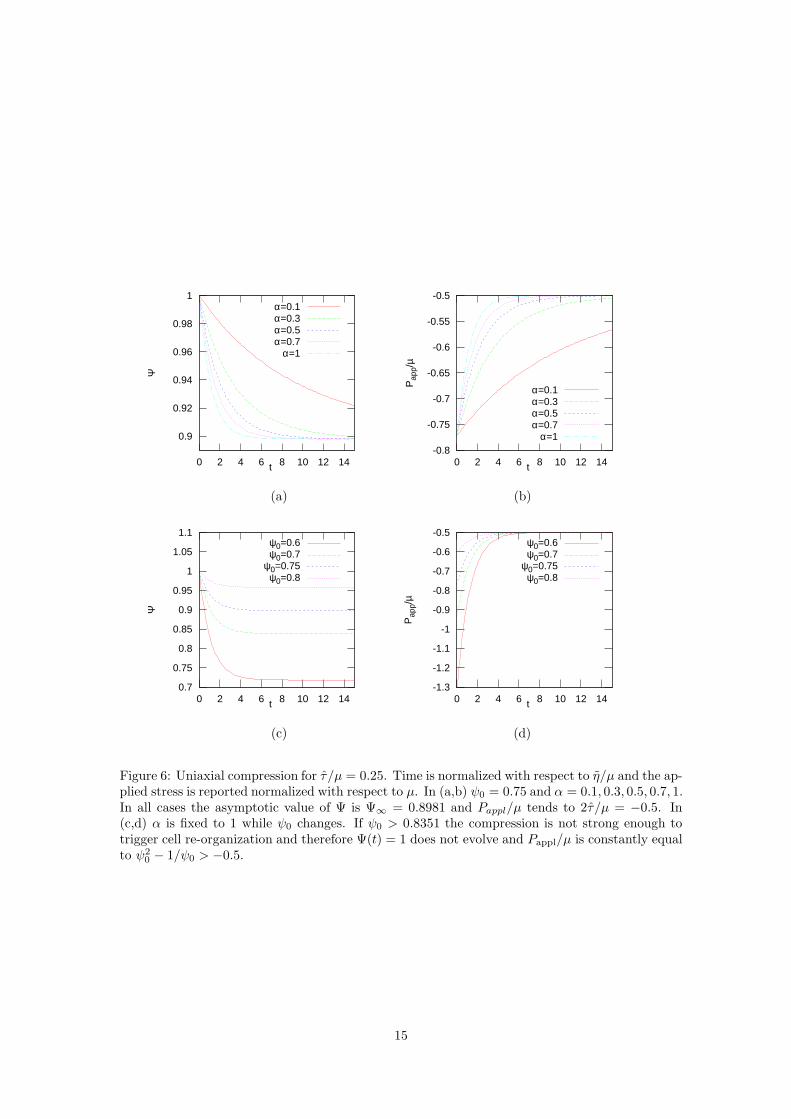
A plot of Ψ(t) is shown in Fig. 6.If the compression applies for a long enough time, then Ψ will tend towards that value Ψ∞ > ψ0

corresponding to the vanishing of the square parenthesis in (4.24), i.e.,

Ψ3∞ − ψ3

0

ψ0Ψ2∞

=2τ

µ, (4.25)

14

0.9

0.92

0.94

0.96

0.98

1

0 2 4 6 8 10 12 14

Ψ

t

α=0.1α=0.3α=0.5α=0.7

α=1

-0.8

-0.75

-0.7

-0.65

-0.6

-0.55

-0.5

0 2 4 6 8 10 12 14

Pap

p/µ

t

α=0.1α=0.3α=0.5α=0.7

α=1

(a) (b)

0.7

0.75

0.8

0.85

0.9

0.95

1

1.05

1.1

0 2 4 6 8 10 12 14

Ψ

t

ψ0=0.6ψ0=0.7

ψ0=0.75ψ0=0.8

-1.3

-1.2

-1.1

-1

-0.9

-0.8

-0.7

-0.6

-0.5

0 2 4 6 8 10 12 14

Pap

p/µ

t

ψ0=0.6ψ0=0.7

ψ0=0.75ψ0=0.8

(c) (d)

Figure 6: Uniaxial compression for τ /µ = 0.25. Time is normalized with respect to η/µ and the ap-plied stress is reported normalized with respect to µ. In (a,b) ψ0 = 0.75 and α = 0.1, 0.3, 0.5, 0.7, 1.In all cases the asymptotic value of Ψ is Ψ∞ = 0.8981 and Pappl/µ tends to 2τ/µ = −0.5. In(c,d) α is fixed to 1 while ψ0 changes. If ψ0 > 0.8351 the compression is not strong enough totrigger cell re-organization and therefore Ψ(t) = 1 does not evolve and Pappl/µ is constantly equalto ψ2

0 − 1/ψ0 > −0.5.

15

that is independent of α, as also evident from Figures 6a.In particular, Pappl will tend to

Pappl,∞ = µψ3

0 − Ψ3∞

ψ0Ψ2∞

= −2τ , (4.26)

(see Fig. 6b,d) that in addition of being independent of α is also independent of ψ0 as in theexperiments in [11].

In Fig. 6c,d instead the value of α is fixed to 1 and different compressions are applied. Ifψ0 > 0.8351 the compression is not strong enough to trigger cell re-organization and thereforeΨ(t) = 1 does not evolve and |Pappl| is constantly below the yielding value that in this case is2τ = 0.5. For larger ψ0 the natural configuration evolves and Pappl again tends to the constantvalue given in (4.26).

The behavior of the solution is then similar to the shear tests discussed in Section 4.4. Finally,if at time t2 (when Ψ = Ψ2 > Ψ∞), the compression is suddenly released, then ψ will readilyadjust to the value ψ = Ψ2.

Although this solution strictly applies to a parallelepiped sample, we qualitatively compare itwith the stress relaxation tests performed by Forgacs et al. [11] for a spheroid. The main remark isthat the measured stress decreases asymptotically to a non-null value that depends on the tissue.

They interpret this long time behavior as the effect of surface tension that can be obtainedmultiplying the measured stress by a coefficient that depends on the geometry of the barrel shapeof the deformed aggregate. In Winters et al. [42] it is observed that doubling the deformation willgive rise to the similar surface tension coefficient, while a constitutive model for a linear elasticsolid whould give rise to a doubling of the stress.

In our view the same result can be interpreted using the constitutive model above and relatingthe asymptotic behavior to a measure of the yield stress. In fact, similarly to the experimentsabove, in the present virtual experiment (that does not present a free boundary) doubling thedeformation will give rise to the same asymptotic value measuring the yield stress.

The relation between the two interpretations is given by τ = Hσ where σ is the surfacetension and H is the mean curvature of the compressed spheroids. Though it is difficult to getthe geometrical parameters from the paper, using the values in Forgacs et al. [11] it seems thatthe yield stress for the different tissues tested ranges between 1 to 100 Pa. Our results for a60% concentration (the maximum one that we used) give a yield stress around 2Pa, and higherconcentrations will probably lead to data in the same range, especially since the yield stress isconcentrated dependent like τ ∼ φ11, as observed previously.

Furthermore, Foty and Steinberg [14] correlate the surface tension coefficient with the density ofsurface cadherin per cell. The same proportionality obviously holds for the yield stress τ becausethis coefficient is clearly related to the number of adhesion bonds. In our opinion the relationbetween yield stress and surface tension also explains the observation by Winters et al [42] thatcell invasiveness is related to the inverse of surface tension: the smaller the adhesion between cells,the smaller the yield stress, the more invasive the cell clone.

We finally mention that Forgacs et al. [11] point out the existence of two relaxation times inthe cellular matter (one of the order of few seconds the other of the order of tens of seconds),that in our approach would be related to two re-organization mechanisms or to the detachmentof different types of adhesion proteins. Of course, our model can be generalized to include morerelaxation times.

5 Conclusions and Developments

In this paper we have derived a constitutive model that is able to describe the twin characteristicsof cell aggregates: solid-like when and where the stresses are not large enough and liquid-likewhen and where the stress overcomes a sustainable threshold inducing internal cell re-organization.Though the constitutive model is kept as simple as possible, we have shown how it can reproducethe outcome of both shear tests performed by [20] and compression tests performed by [11, 13,

16

12, 14, 42]. The model also enabled us to predict the nonlinear dynamic shear behavior as oftenencountered with complex fluids. In addition, a comparison between the surface tension conceptand the yield stress concept allowed to explain the relationship between cell invasiveness and yieldstress (or surface tension) described in [42], i.e., the smaller the adhesion between cells, the smallerthe yield stress the more invasive is the cell clone.

The theoretical basis of this work are the yield stress exhibited by cell suspensions (at acontinuum level) and the energy needed to break the adhesion bonds of a cell on an aggregate(at a cell level). On the basis of this experimental evidence, in this paper we have conjecturedthat also cell aggregates can exhibit a yield adhesion reflecting itself, at a continuum level, ina threshold tension separating an elastic and a viscous regime. The comparison with the veryfew experiments on cell aggregates present in the literature suggests that this volumetric theorycould provide an explanation to the ability of cell aggregates to carry loadsi, alternative to surfacetension. Even more important, the re-organization process could explain the permanent strainexhibited by spheroid samples after load.

Of course, the model can and need to be improved in several directions in order to reproducemore closely the behavior of cell aggregates. For instance, one should take into account the factthat the cell aggregate is a porous material filled with the liquid in which the experiment is done.Such an effect can be easily included by adding a further viscous component to the mechanicalbehavior of the cellular constituent. This is particularly important to explain creeping phenomenaoccurring when external stresses applied on the cellular aggregate are suddenly applied or released.

Another extension can be represented by the inclusion of more cell re-arrangement times, thatcan be related to different adhesion mechanisms. These can be due not only to different types ofadhesion molecules at the cell membranes but also to the response occurring inside the cell itselfwith the rearrangement of the adhesion bonds connected to the actin cytoskeleton. In this casealso the active role of myosin should be taken into account as well. In addition, more experimentsneed to be done to understand the origin of the exponent α either using different types of cells,or interphering with the adhesion mechanisms, and to find its dependence on cell concentration.

Deducing a model with more relaxation times would probably lead to a better fit of the ex-periments by [11, 13, 12, 14]. Nevertheless, the model provided here is a three-dimensional one,different from previous studies [11] suggesting to use simple one–dimensional Maxwell assemblies,coupled with the presence of an arbitrary surface tension. Here we provide a complete descriptionof this visco-elasto-plastic model, and possible parameters have been chosen based on experimentaldata [20], this leading to relaxation constants in the range of the ones obtained previously [11].

Appendix

In this appendix we will briefly discuss some aspects of kinematics that are useful to deducethe constitutive equation proposed in Section 2. In doing that, one needs to compute the timederivative of the elastic constitutive model

T′ = µ

(

Bn − 1

3trBnI

)

, (5.1)

which implies to compute the time derivative of Bn = FnFTn . This gives

Bn = LnBn + BnLTn , (5.2)

whereLn = FnF

−1n . (5.3)

In the following we will also use the following tensors

L = FF−1 and Lp = FpF

−1p . (5.4)

Deriving F in time, one has

F = FnFp + FnFp = LnFnFp + FnFpF−1p F

−1n FnFp = (Ln + FnLpF

−1n )F , (5.5)

17

that, using the definition (5.4) can be rewritten as

Ln = L − FnLpF−1n . (5.6)

Back substitution of (5.6) into (5.2) gives

Bn = LBn + BnLT − 2FnDpF

Tn , (5.7)

where

Dp =1

2(Lp + L

Tp ) , (5.8)

orDBn

Dt= −2FnDpF

Tn , (5.9)

where DM/Dt is the Maxwell upper convected derivative (2.14).In this way, we related the evolution of T′ to the evolution of Bn and through Dp to the

evolution of the natural configuration. On the other hand, in Section 2 we also introduced theequation governing the evolution of the natural configuration

FnDpF−1n =

1

2η

[

1 − 1

f(T′)

]

+

T′ , (5.10)

where [·]+ stands for the positive part of the argument.Notice that, coherently with the fact that the l.h.s. of (5.10) is traceless as T′

tr(FnDpF−1n ) = tr Dp = 0 . (5.11)

In fact, the assumption that the volume ratios in the natural and in the original reference con-figuration are the same implies Jp ≡ det Fp = 1. Therefore, from standard tensor calculus, onehas

Jp = Jptr Dp = 0 , (5.12)

which means that Dp is traceless.We conclude this appendix by observing that one can re-write (5.10) as

1 − 1

f(

S′

nCn

Jn

)

+

S′nCn

Jn= 2ηDp , (5.13)

where S′n = JnF−1

n T′F−Tn is the (excess) second Piola-Kirchhoff stress tensor and Cn = FT

nFn. Itcan be noticed that since

tr(S′nCn) = tr(JnF

−1n T

′Fn) = JntrT′ = 0 (5.14)

S′nCn is traceless as Dp.

In addition, if we assume that the cellular spheroid obeys a neo-Hookean law,

T = µ(φ)(−ΣI + Bn) (5.15)

where Σ = Σ(φ/φn), with Σ(1) = 1, thenS′

nCn

Jnhas the same eigenvalues as T′ so that f

(

S′

nCn

Jn

)

=

f(T′), and µ(φ) is the shear elastic modulus.

18

References

[1] D. Ambrosi and F. Mollica. On the mechanics of a growing tumour. Int. J. Engng. Sci.,40:1297–1316, 2002.

[2] D. Ambrosi and L. Preziosi. Cell adhesion mechanisms and stress relaxation in the mechanicsof tumours. Biomech. Model. Mechanobiol., in press, 2009.

[3] I. V. Basov and V. V. Shelukhin. Generalized solutions to the equations of compressiblebingham flows. Z. Angew. Math. Mech., 79:185–192, 1999.

[4] G. I. Bell, M. Dembo, and P. Bongrand. Cell adhesion. competition between nonspecificrepulsion and specific bonding. Biophys. J., 45(6):1051–1064, 1984.

[5] D. A. Beysens, G. Forgacs, and J. A. Glazier. Cell sorting is analogous to phase ordering influids. Proc. Natl. Acad. Sci. USA, 97(17):9467–9471, 2000.

[6] R. B. Bird, R. C. Armstrong, and O. Hassager. Dynamics of polymeric liquids. Volume 1.Fluid mechanics (2nd edition). John Wiley and sons, 1987.

[7] R. Buscall, P. D. A. Mills, J. W. Goodwin, and D. W. Lawson. Scaling behaviour of therheology of aggregate networks formed from colloidal particles. J. Chem. Soc. Faraday Trans.,84:4249–4260, 1988.

[8] S. Chien, S. Usami, R. J. Dellenback, and M. I. Gregersen. Blood viscosity: influence oferythrocyte deformation. Science, 157:827–829, 1967.

[9] S. Chien, S. Usami, R. J. Dellenback, M. I. Gregersen, L. B. Nanninga, and M. Mason-Guest.Blood viscosity: influence of erythrocyte aggregation. Science, 157:829–831, 1967.

[10] S. Chien, S. Usami, H. M. Taylor, J. L. Lundberg, and M. I. Gregersen. Effects of hematocritand plasma proteins on human blood rheology at low shear rates. J. Appl. Physiology, 21:81–87, 1966.

[11] G. Forgacs, R. A. Foty, Y. Shafrir, and M. S. Steinberg. Viscoelastic properties of livingembryonic tissues: a quantitative study. Biophys. J., 74(5):2227–2234, 1998.

[12] R. A. Foty, G. Forgacs, Pfleger, and M. S. Steinberg. Surface tensions of embryonic tissuespredict their mutual envelopment behavior. Development, 122:1611–1620, 1996.

[13] R. A. Foty, G. Forgacs, C. M. Pfleger, and M. S. Steinberg. Liquid properties of embryonictissues: Measurement of interfacial tensions. Phys. Rev. Letters, 72(14):2298–2301, 1994.

[14] R. A. Foty and M. S. Steinberg. The differential adhesion hypothesis: a direct evaluation.Dev. Biol., 278(1):255–263, 2005.

[15] S. J. Franks, H. M. Byrne, J. R. King, J. C. E. Underwood, and C. E. Lewis. Modelling theearly growth of ductal carcinoma in situ of the breast. J. Math. Biol., 47:424–452, 2003.

[16] S. J. Franks, H. M. Byrne, H. S. Mudhar, J. C. E. Underwood, and C.E. Lewis. Mathematicalmodelling of comedo ductal carcinoma in situ of the breast. Math. Med. Biol., 20:277–308,2003.

[17] Y. C. Fung. Microrheology and constitutive equation of soft tissue. Biorheology, 25:261–270,1978.

[18] R. F. Gibson. Principles of Composite Material Mechanics. Mc Graw-Hill, 1994.

[19] K. Hyun, S. H. Kim, K. H. Ahn, and S. J. Lee. Large amplitude oscillatory shear as a wayto classify the complex fluids. J. Non-Newtonian Fluid Mech., 107:51–65, 2002.

19

[20] A. Iordan, A. Duperray, and C. Verdier. Fractal approach to the rheology of concentratedcell suspensions. Phys. Rev. E, 77(1):011911, 2008.

[21] D. D. Joseph. Fluid Dynamics of Viscoelastic Liquids. Springer, 1990.

[22] E. Kroener. Allgemeine kontinuumstheorie der versetzungen und eigenspannungen. Arch.Rational Mech. Anal., 4:273–334, 1960.

[23] E. Lee. Elastic-plastic deformation at high strains. J. Applied Mechanics, 36:1–6, 1969.

[24] W. A. Malik, S. C. Prasad, K. R. Rajagopal, and L. Preziosi. On the modelling of theviscoelastic response of embryonic tissues. Math. Mech. Solids, 13:81–91, 2008.

[25] L. E. Malvern. Introduction of the Mechanics of a Continuous Medium. Prentice Hall Inc.,1969.

[26] J. C. M. Mombach and J. A. Glazier. Single cell motion in aggregates of embryonic cells.Phys. Rev. Letters, 76:3032–3035, 1996.

[27] J. C. M. Mombach, D. Robert, F. Graner, G. Gillet, G. L. Thomas, M. Idiart, and J. P.Rieu. Rounding of aggregates of biological cells: Experiments and simulations. Physica A,352:525–534, 2005.

[28] H. M. Phillips and M. S. Steinberg. Embryonic tissues as elasticoviscous liquids. i. rapid andslow shape changes in centrifuged cell aggregates. J. Cell. Sci., 30:1–20, 1978.

[29] H. M. Phillips, M. S. Steinberg, and B. H. Lipton. Embryonic tissues as elasticoviscous liquids.ii. direct evidence for cell slippage in centrifuged aggregates. Develop. Biol., 59:124–134, 1977.

[30] L. Preziosi. On an invariance property of the solution to stokes’ first problem for viscoelasticfluids. J. Non-Newtonian Fluid Mech., 33:225–228, 1989.

[31] L. Preziosi and D. D. Joseph. Stokes’ first problem for viscoelastic fluids. J. Non-NewtonianFluid Mech., 25:239–259, 1987.

[32] S. Reynaert, P. Moldenaers, and J. Vermant. Interfacial rheology of stable and weakly aggre-gated two-dimensional suspensions. Phys. Chem. Chem. Phys., 9:6463–6475, 2007.

[33] J. P. Rieu, K. Tsuchiya, S. Sawai, Y. Maeda, and Y. Sawada. Cell movements and tractionforces during the migration of 2-dimensional dictyostelium slugs. J. Biol. Phys., 29:1–4, 2003.

[34] J. P. Rieu, A. Upadhyaya, J. A. Glazier, N. B. Ouchi, and Y. Sawada. Diffusion and defor-mations of single hydra cells in cellular aggregates. Biophys. J., 79:1903–1914, 2000.

[35] P. Saramito. A new constitutive equation for elastoviscoplastic fluid flows. J. Non-NewtonianFluid Mech., 145:1–14, 2007.

[36] P. Saramito. A new elastoviscoplastic model based on the herschel-bulkley viscoplasticity. J.Non-Newtonian Fluid Mech., 158:154–161, 2009.

[37] P. Snabre, M. Bitbol, and P. Mills. Cell disaggregation behavior in shear flow. Biophys. J.,51(5):795–807, 1987.

[38] P. Snabre and P. Mills. I. rheology of weakly flocculated suspensions of rigid particles. J.Phys. III. France, 6:1811–1834, 1996.

[39] W. Supatto, D. Debarre, B. Moulia, E. Brouzes, J.L. Martin, E. Farge, and E. Beaurepaire.In vivo modulation of morphogenetic movements in drosophila embryos with femtosecondlaser pulses. Proc. Natl. Acad. Sci. USA, 102(4):1047–1052, 2005.

[40] G. B. Thurston. Viscoelasticity of human blood. Biophys. J., 12:1205–1217, 1972.

20

[41] C. Verdier. Review. rheological properties of living materials: From cells to tissues. J. Theor.Med., 5(2):67–91, 2003.

[42] B. S. Winters, S. R. Shepard, and R. A. Foty. Biophysical measurement of brain tumorcohesion. Int. J. Cancer, 114(3):371–379, 2005.

21