An Economic Examination of Collateralization in

Different Financial Markets

Tim Xiao1

ABSTRACT

This paper attempts to assess the economic significance and implications of collateralization in

different financial markets, which is essentially a matter of theoretical justification and empirical

verification. We present a comprehensive theoretical framework that allows for collateralization adhering

to bankruptcy laws. As such, the model can back out differences in asset prices due to collateralized

counterparty risk. This framework is very useful for pricing outstanding defaultable financial contracts.

By using a unique data set, we are able to achieve a clean decomposition of prices into their credit risk

factors. We find empirical evidence that counterparty risk is not overly important in credit-related spreads.

Only the joint effects of collateralization and credit risk can sufficiently explain unsecured credit costs.

This finding suggests that failure to properly account for collateralization may result in significant

mispricing of financial contracts. We also analyze the difference between cleared and OTC markets.

Key words: unilateral/bilateral collateralization, partial/full/over collateralization, asset pricing, plumbing

of the financial system, swap premium spread, OTC/cleared/listed financial markets.

JEL Classification: E44, G21, G12, G24, G32, G33, G18, G28

1 Risk Quant, Capital Markets, CIBC, 161 Bay Street, 10

th Floor, Toronto, ON M5J 2S8, Canada;

email: tim_yxiao@yahoo.com Url: https://finpricing.com/

1

1. Introduction

Collateralization is an essential element in the so-called plumbing of the financial system that is

the Achilles' heel of global financial markets. It allows financial institutions to reduce economic capital

and credit risk, free up lines of credit, and expand the range of counterparties. All of these factors

contribute to the growth of financial markets. The benefits are broadly acknowledged and affect dealers

and end users, as well as the financial system generally.

The reason collateralization of financial derivatives and repos has become one of the most

important and widespread credit risk mitigation techniques is that the Bankruptcy Code contains a series

of “safe harbor” provisions to exempt these contracts from the “automatic stay”. The automatic stay

prohibits the creditors from undertaking any act that threatens the debtor’s asset, while the safe harbor, a

luxury, permits the creditors to terminate derivative and repo contracts with the debtor in bankruptcy and

to seize the underlying collateral. This paper focuses on safe harbor contracts (e.g., derivatives and repos),

but many of the points made are equally applicable to automatic stay contracts.

Financial derivatives can be categorized into three types. The first category is over-the-counter

(OTC) derivatives, which are customized bilateral agreements. The second group is cleared derivatives,

which are negotiated bilaterally but booked with a clearinghouse. Finally, the third type is exchange-

traded/listed derivatives, which are executed over an exchange. The differences between the three types

are described in detail on the International Swap Dealers Association (ISDA) website (see ISDA (2013)).

Under the new regulations (e.g., Dodd-Frank Wall Street Reform Act), certain ‘eligible’ OTC

derivatives must be cleared with central counterparties (CCPs) (see Heller and Vause (2012), Pirrong

(2011), etc.). Hull (2011) further recommends mandatory CCP clearing of all OTC derivatives.

Meanwhile, Duffie and Zhu (2011) suggest a move toward the joint clearing of interest rate swaps and

credit default swaps (CDS) in the same clearinghouse.

The posting of collateral is regulated by the Credit Support Annex (CSA). The CSA was

originally designed for OTC derivatives, but more recently has been updated for cleared/listed derivatives.

2

For this reason people in the financial industry often refer to collateralized contracts as CSA contracts and

non-collateralized contracts as non-CSA contracts.

There are three types of collateralization: full, partial or over. Full-collateralization is a process

where the posting of collateral is equal to the current mark-to-market (MTM) value. Partial/under-

collateralization is a process where the posting of collateral is less than the current MTM value. Over-

collateralization is a process where the posting of collateral is greater than the current MTM value.

From the perspective of collateral obligations, collateral arrangements can be unilateral or

bilateral. In a unilateral arrangement, only one predefined counterparty has the right to call for collateral.

Unilateral agreements are generally used when the other counterparty is much less creditworthy. In a

bilateral arrangement, on the other hand, both counterparties have the right to call for collateral.

Upon default and early termination, the values due under the ISDA Master Agreement are

determined. These amounts are then netted and a single net payment is made. All of the collateral on hand

would be available to satisfy this total amount, up to the full value of that collateral. In other words, the

collateral to be posted is calculated on the basis of the aggregated value of the portfolio, but not on the

basis of any individual transaction.

The use of collateral in financial markets has increased sharply over the past decade, yet

analytical and empirical research on collateralization is relatively sparse. The effect of collateralization on

financial contracts is an understudied area. Collateral management is often carried out in an ad-hoc

manner, without reference to an analytical framework. Comparatively little research has been done to

analytically and empirically assess the economic significance and implications of collateralization. Such a

quantitative and empirical analysis is the primary contribution of this paper.

Due to the complexity of quantifying collateralization, previous studies seem to turn away from

direct and detailed modeling of collateralization (see Fuijii and Takahahsi (2012)). For example, Johannes

and Sundaresan (2007), and Fuijii and Takahahsi (2012) characterize collateralization via a cost-of-

collateral instantaneous rate (or stochastic dividend or convenience yield). Piterbarg (2010) regards

3

collateral as a regular asset in a portfolio and uses the replication approach to price collateralized

contracts. All of the previous works focus on full-collateralization only.

We obtain the CSA data from two investment banks. The data show that only 8.92% of CSA

counterparties are subject to unilateral collateralization, while the remaining 91.08% are bilaterally

collateralized. The data also reveal that all contracts in OTC markets are partially collateralized due to the

mechanics of CSAs, which allow for the existence of limited unsecured exposures and set minimum

transfer amounts (MTAs), whereas all contracts in cleared/listed markets are over-collateralized as all

CCPs/Exchanges require initial margins. Therefore, full-collateralization does not exist in the real world2.

The reason for the popularity of full-collateralization is its mathematical simplicity and tractability.

This article makes a theoretical and empirical contribution to the study of collateralization by

addressing several essential questions concerning the posting of collateral. First, how does

collateralization affect expected asset prices? To answer this question, we develop a comprehensive

analytical framework for pricing financial contracts under different (partial/full/over and unilateral

/bilateral) collateral arrangements in different (OTC/cleared/listed) markets.

In contrast to other collateralization models in current literature, we characterize a collateral

process directly based on the fundamental principal and legal structure of the CSA agreement. A model is

devised that allows for collateralization adhering to bankruptcy laws. As such, the model can back out

differences in prices due to counterparty risk. This framework is very useful for valuing off-the-run or

outstanding financial contracts subject to credit risk and collateralization, where the price quotes are not

available. Given this model, we are able to explain credit-related spreads and provide an important tool

for credit value adjustment (CVA).

Our theoretical analysis shows that collateralization can always improve recovery and reduce

credit risk. If a contract is over-collateralized (e.g., a repo or cleared contract), its value is equal to the

2 Singh (2010) and ECB (2009) come to a similar conclusion, although they do not provide any data to

justify their statements.

4

risk-free value. If a contract is partially collateralized (e.g., an OTC derivatives), its CSA value is less

than the risk-free value but greater than the non-CSA risky value.

Second, how can the model be empirically verified? To achieve the verification goal, this paper

empirically measures the effect of collateralization on pricing and compares it with model-implied prices.

This calls for data on financial contracts that have different collateral arrangements but are similar

otherwise. We use a unique interest rate swap contract data set from an investment bank for the empirical

study, as interest rate swaps collectively account for around two-thirds of both the notional and market

value of all outstanding derivatives.

ISDA mid-market swap rates quoted in the market are based on hypothetical counterparties of

AA-rated quality or better. Dealers use this market rate as a reference when quoting an actual swap rate to

a client and make adjustments based on many factors, such as credit risk, liquidity risk, funding cost,

operational cost and expected profit, etc. Unlike most other studies, this study mainly concentrates the

analysis on swap adjustments/premia related to credit risk and collateralization, which are to be made to

the mid-market swap rates for real counterparties.

Prior research has primarily focused on the generic mid-market swap rates and results appear

puzzling. Sorensen and Bollier (1994) believe that swap spreads (i.e., the difference between swap rates

and par yields on similar maturity Treasuries) are partially determined by counterparty default risk.

Whereas Duffie and Huang (1996), Hentschel and Smith (1997), Minton (1997) and Grinblatt (2001) find

weak or no evidence of the impact of counterparty credit risk on swap spreads. Collin-Dufresne and

Solnik (2001) and He (2001) further argue that many credit enhancement devices, e.g., collateralization,

have essentially rendered swap contracts risk-free. Meanwhile, Duffie and Singleton (1997), and Liu,

Longstaff and Mandell (2006) conclude that both credit and liquidity risks have an impact on swap

spreads. Moreover, Feldhütter and Lando (2008) find that the liquidity factor is the largest component of

swap spreads. It seems that there is no clear-cut answer yet regarding the relative contribution of the

liquidity and credit factors. Maybe, the recently revealed LIBOR scandal can partially explain these

conflicting findings.

5

Unlike the generic mid-market swap rates, swap premia are determined in a competitive market

according to the basic principles of supply and demand. A client who wants to enter a swap contract first

contacts a number of swap dealers and asks for a swap rate. After comparing all quotations, the client

chooses the most competitive rate. A swap premium is supposed to cover operational, liquidity, funding,

and credit costs as well as a profit margin. If the premium is too low, the dealer may lose money. If the

premium is too high, the dealer may lose the competitive advantage.

Unfortunately, we do not know the detailed allocation of a swap premium, i.e., what percentage

of the adjustment is charged for each factor. Thus, a direct empirical verification is impossible.

To circumvent this difficulty, this article uses an indirect process to verify the model empirically.

We define a swap premium spread as the difference between the swap premia of two collateralized swap

contracts that have exactly the same terms and conditions but are traded with different counterparties

under different collateral agreements. We reasonably believe that if two contracts are identical except

counterparties, the premium spread should reflect the difference between two counterparties’ unsecured

credit risks only, as all other risks and costs are identical.

Empirically, we find quite a number of CSA swap pairs in the data, where the two contracts in

each pair have different counterparties but are otherwise the same. The test results demonstrate that the

model-implied swap premium spreads are very close to the market swap premium spreads, indicating that

the model is quite accurate.

Third, what are the effects of counterparty risk and collateralization, alone or combined, on swap

premium spreads? We first study the marginal impact of counterparty risk on spreads. CDS premia (the

prices of insuring against a firm’s default) theoretically reflect the credit risk of the firm. Presumably,

differences in CDS premia should be largely attributable to differences in counterparty risk. We estimate

a regression model where market swap premium spreads are used as the dependent variable and

differences between CDS premia as the explanatory variable. The estimation results show that the

adjusted 2R is 0.7472, implying that approximately 75% of market premium spreads can be explained by

6

CDS spreads. In other words, counterparty risk alone can provide a good but not overwhelming prediction

on spreads.

Next, we assess the joint effect of both counterparty risk and collateralization on premium

spreads. Since the model-generated swap premium spreads take into account both counterparty risk and

collateralization, we present another regression model where the market swap premium spreads are

regressed on the implied swap premium spreads. The estimation results show that the constant term is

insignificantly different from zero; the slope coefficient is close to 1 and the adjusted 2R is very high.

This suggests that the implied premium spreads explains nearly all of the market premium spreads.

Finally, how does collateralization impact pricing in different markets? Our proprietary data

reveal that cleared swaps have dramatically increased since 2011, reflecting the financial institutions’

compliance to regulatory requirements. We find evidence that the economical determination of swap rates

in cleared markets is the same as that in OTC markets, as all clearinghouses claim that cleared derivatives

would replicate OTC derivatives, and promise that transactions through the clearinghouses would be

economically equivalent to similar transactions handled in OTC markets.

Although the practice recommended by CCPs is popular in the market, in which derivatives are

continuously negotiated over-the-counter as usual but cleared and settled through clearinghouses, some

market participants cast doubt on CCPs’ economic equivalence claim. They find that cleared contracts

have actually significant differences when compared with OTC trades. Some firms even file legal action

against the clearinghouses, and accuse them of fraudulently inducing the firms to enter into cleared

derivatives on the premise the contracts would be economically equivalent to OTC contracts (see

Pengelly (2011)).

In fact, our study shows that there are many differences between cleared markets and OTC

markets. After much discussion, we come to the conclusion that cleared derivatives are not economically

equivalent to their OTC counterparts. These discussions may be of interest to regulators, academics and

practitioners.

7

The remainder of this paper is organized as follows: Section 2 discusses unilateral

collateralization. Section 3 elaborates bilateral collateralization. Section 4 presents empirical evidence.

The conclusions and discussion are provided in Section 5. All proofs and some detailed derivations are

contained in the appendices.

2. Unilateral Collateralization

A unilateral collateral arrangement is sometimes used when a higher-rated counterparty deals

with a lower-rated counterparty, in which only one party, normally the lower-rated one, is required to

deliver collateral to guarantee performance under the agreement. Typical examples of unilaterally

collateralized contracts include: repos, cleared/listed derivatives, sovereign derivatives (see AFME-

ICMA-ISDA (2011)), and some OTC derivatives3.

We consider a filtered probability space ( , F , 0ttF , P ) satisfying the usual conditions,

where denotes a sample space, F denotes a -algebra, P denotes a probability measure, and

0ttF denotes a filtration.

Since the only reason for taking collateral is to reduce/eliminate credit risk, collateralization

analysis is closely related to credit risk modeling. There are two primary types of models that attempt to

describe default processes in the literature: structural models and reduced-form models. Many people in

the market have tended to gravitate toward the reduced-from models given their mathematical tractability

and market consistency. In the reduced-form framework, the stopping (or default) time of a firm is

modeled as a Cox arrival process (also known as a doubly stochastic Poisson process) whose first jump

occurs at default and is defined by,

t

s dssht0

),(:inf (1)

3 Our CSA data from two investment banks show that 8.92% of CSA counterparties are subject to

unilateral collateralization

8

where )(th or ),( tth denotes the stochastic hazard rate or arrival intensity dependent on an exogenous

common state t , and is a unit exponential random variable independent of

t .

It is well-known that the survival probability from time t to s in this framework is defined by

s

tduuhtsPstp )(exp)|(:),( (2a)

The default probability for the period (t, s) in this framework is given by

s

tduuhstptsPstq )(exp1),(1)|(:),( (2b)

In order to assess the impact of collateralization on pricing, we study valuation with and without

collateralization respectively.

2.1 Valuation without collateralization

Let valuation date be t. Consider a financial contract that promises to pay a 0TX from party B

to party A at maturity date T, and nothing before date T. We suppose that party A and party B do not have

a CSA agreement. All calculations are from the perspective of party A. The risk free value of the financial

contract is given by

tFTF XTtDEtV ),()( (3a)

where

duurTtD

T

t)(exp),( (3b)

where tE F is the expectation conditional on the tF , ),( TtD denotes the risk-free discount factor at

time t for the maturity T and )(ur denotes the risk-free short rate at time u ( Tut ).

Next, we discuss risky valuation. In a unilateral credit risk case, we assume that party A is

default-free and party B is defaultable. We divide the time period (t, T) into n very small time intervals

( t ). In our derivation, we use the approximation yy 1exp provided that y is very small. The

survival and default probabilities of party B for the period (t, tt ) are given by

9

tthtthtttptp )(1)(exp),(:)(ˆ (4a)

tthtthtttqtq )()(exp1),(:)(ˆ (4b)

The binomial default rule considers only two possible states: default or survival. For the one-

period (t, tt ) economy, at time tt the contract either defaults with the default probability

),( tttq or survives with the survival probability ),( tttp . The survival payoff is equal to the

market value )( ttV N and the default payoff is a fraction of the market value4: )()( ttVtt N ,

where is the recovery rate. The non-CSA value of the contract at time t is the discounted expectation of

all possible payoffs and is given by

tN

tNN ttVttbEttVtqttpttrEtV FF )()(exp)()(ˆ)()(ˆ)(exp)( (5)

where )()()(1)()()( tstrtthtrtb denotes the (short) risky rate and )(1)()( tthts denotes

the (short) credit spread.

Similarly, we have

ttNN ttVtttbEttV F)2()(exp)( (6)

Note that ttb )(exp is ttF -measurable. By definition, an ttF -measurable random

variable is a random variable whose value is known at time tt . Based on the taking out what is

known and tower properties of conditional expectation, we have

t

N

i

tttN

tNN

ttVttitbE

ttVtttbEttbEttVttbEtV

F

FFF

)2())(exp

)2()(exp)(exp)()(exp)(

1

0

(7)

By recursively deriving from t forward over T where TN XTV )( and taking the limit as t

approaches zero, the non-CSA value of the contract can be obtained as

tT

T

t

N XduubEtV F)(exp)( (8)

4 Here we use the recovery of market value (RMV) assumption.

10

We may think of )(ub as the risk-adjusted short rate. Equation (8) is the same as Equation (10) in

Duffie and Singleton (1999), which is the market model for pricing risky bonds.

In theory, a default may happen at any time, i.e., a risky contract is continuously defaultable. This

Continuous Time Risky Valuation Model is accurate but sometimes complex and expensive. For

simplicity, people sometimes prefer the Discrete Time Risky Valuation Model that assumes that a default

may only happen at some discrete times. A natural selection is to assume that a default may occur only on

the payment dates. Fortunately, the level of accuracy for this discrete approximation is well inside the

typical bid-ask spread for most applications (see O’Kane and Turnbull (2003)). From now on, we will

focus on the discrete setting only, but many of the points we make are equally applicable to the

continuous setting.

If we assume that a default may occur only on the payment date, the non-CSA value of the

instrument in the discrete-time setting is given by

tt FF TTN XTtIEXTtqTTtpTtDEtV ),(),()(),(),()( (9)

where ),()(),(),(),( TtqTTtpTtDTtI can be regarded as a risk-adjusted discount factor.

The difference between the risk-free value and the risky value is known as the credit value

adjustment (CVA). CVA is required by regulators, such as, International Accounting Standard Board

(IASB) and Basel committee. The CVA reflects the market value of counterparty risk or the cost of

protection required to hedge counterparty risk and is given by

tFTNF XTTtqTtDEtVtVtCVA )(1),(),()()()( (10)

Since the recovery rate is always less than 1, we have 0)( tCVA or FN VtV )( . In other words,

the risky value is always less than the risk-free value. An intuitive explanation is that credit risk makes a

financial contract less valuable.

2.2 Valuation with collateralization

The posting of collateral is regulated by the CSA that specifies a variety of terms including the

threshold, the independent amount, and the minimum transfer amount (MTA), etc. The threshold is the

11

unsecured credit exposure that a party is willing to bear. The MTA is used to avoid the workload

associated with a frequent transfer of insignificant amounts of collateral. The independent amount plays

the same role as the initial margin (or haircut).

We define effective collateral threshold as the threshold plus the MTA. The collateral is called as

soon as the mark-to-market (MTM) value rises above the effective threshold. A positive effective

threshold corresponds to partial/under-collateralization where the posting of collateral is less than the

MTM value. A negative effective threshold represents over-collateralization where the posting of

collateral is greater than the MTM value. A zero-value effective threshold equates with full-

collateralization where the posting of collateral is equal to the MTM value.

Suppose that there is a unilateral CSA agreement between parties A and B in which only party B

is required to deliver collateral when the mark-to-market (MTM) value arises over the collateral threshold

H.

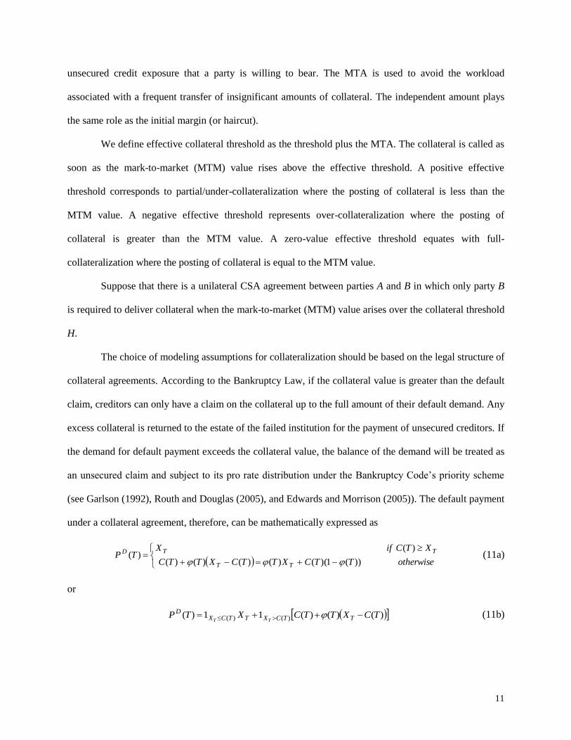
The choice of modeling assumptions for collateralization should be based on the legal structure of

collateral agreements. According to the Bankruptcy Law, if the collateral value is greater than the default

claim, creditors can only have a claim on the collateral up to the full amount of their default demand. Any

excess collateral is returned to the estate of the failed institution for the payment of unsecured creditors. If

the demand for default payment exceeds the collateral value, the balance of the demand will be treated as

an unsecured claim and subject to its pro rate distribution under the Bankruptcy Code’s priority scheme

(see Garlson (1992), Routh and Douglas (2005), and Edwards and Morrison (2005)). The default payment

under a collateral agreement, therefore, can be mathematically expressed as

otherwiseTTCXTTCXTTC

XTCifXTP

TT

TTD

))(1)(()()()()(

)()(

(11a)

or

)()()(11)( )()( TCXTTCXTP TTCXTTCXD

TT (11b)

12

where Y is an indicator function that is equal to one if Y is true and zero otherwise, and C(T) is the

collateral amount at time T.

It is worth noting that the default payment in equation (11) is always greater than the original

recovery, i.e., TD XTTP )()( , since )(T is always less than 1. Said differently, the default payoff of a

CSA contract is always greater than the default payoff of the same contract without a CSA agreement.

That is why the major benefit of collateralization should be viewed as an improved recovery in the event

of a default.

Let us consider repo/cleared/listed markets first. Contracts in these markets are always over

collateralized, as the parties with collateral obligation are required to deposit initial margins and are also

charged variation margins in response to changes in the market values. The total collateral (initial margin

plus variation margin) posted at time t is given by

)()()( tHtVtC C (12)

where )(tV C is the CSA value of the contract at time t and )(tH is the effective threshold. Note that for

over-collateralization, the effective threshold is negative, i.e., 0)( tH , which equals the negative initial

margin. The collateral in equation (12) is a linear function of the asset value.

In general, initial margins are set very conservatively so that they are sufficient to cover losses

under all scenarios considered. Also, the initial margins can be adjusted in response to elevated price

volatility. Moreover, daily marking-to-market and variation margin settlement can further eliminate the

risk that a loss exceeds the collateral amount. Thus, it is reasonable to believe that under over-

collateralization the collateral amount is always greater than the default claim, i.e., TXTC )( .

At time T, if the contract survives with probability ),( Ttp , the survival value is the promised

payoff TX and the collateral taker returns the collateral to the collateral provider. If the contract defaults

with probability ),( Ttq , the collateral taker has recourse to the collateral and obtains a default payment

up to the full value of the promised payoff TX . The remaining collateral TXTC )( returns to the

13

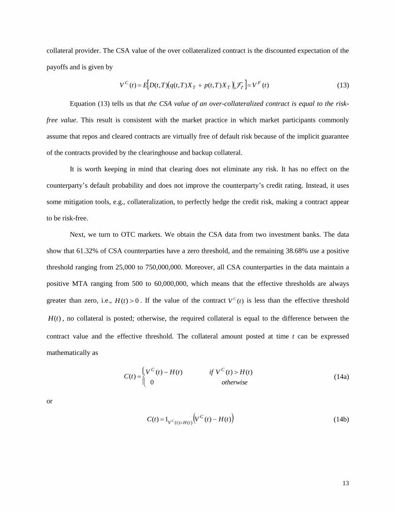
collateral provider. The CSA value of the over collateralized contract is the discounted expectation of the

payoffs and is given by

)(),(),(),()( tVXTtpXTtqTtDEtV FTT

C tF (13)

Equation (13) tells us that the CSA value of an over-collateralized contract is equal to the risk-

free value. This result is consistent with the market practice in which market participants commonly

assume that repos and cleared contracts are virtually free of default risk because of the implicit guarantee

of the contracts provided by the clearinghouse and backup collateral.

It is worth keeping in mind that clearing does not eliminate any risk. It has no effect on the

counterparty’s default probability and does not improve the counterparty’s credit rating. Instead, it uses

some mitigation tools, e.g., collateralization, to perfectly hedge the credit risk, making a contract appear

to be risk-free.

Next, we turn to OTC markets. We obtain the CSA data from two investment banks. The data

show that 61.32% of CSA counterparties have a zero threshold, and the remaining 38.68% use a positive

threshold ranging from 25,000 to 750,000,000. Moreover, all CSA counterparties in the data maintain a

positive MTA ranging from 500 to 60,000,000, which means that the effective thresholds are always

greater than zero, i.e., 0)( tH . If the value of the contract )(tV C is less than the effective threshold

)(tH , no collateral is posted; otherwise, the required collateral is equal to the difference between the

contract value and the effective threshold. The collateral amount posted at time t can be expressed

mathematically as

otherwise

tHtViftHtVtC

CC

0

)()()()()( (14a)

or

)()(1)()()(

tHtVtC C

tHtV C

(14b)

14

In contrast to repo/cleared markets, collateral posted in OTC markets is a nonlinear function of

daily market value changes. In fact, this discontinuous and state-dependent indicator function is the root

cause of the complexity of collateralized valuation in OTC markets.

Since all CSA derivatives in OTC markets are partially collateralized, the default claim is almost

certainly greater than the collateral amount. For a discrete one-period (t, T) economy, the collateral

amount )(tC posted at time t is defined in (14). At time T, if the contract survives, the survival value is

the promised payoff TX and the collateral taker returns the collateral to the collateral provider. If the

contract defaults, the collateral taker possesses the collateral. The portion of the default claim that exceeds

the collateral value is treated as an unsecured claim. Thus, the default payment is )()()( TCXTTC T ,

where ),(/)()( TtDtCTC is the future value of the collateral. Since the most predominant form of

collateral is cash according to ISDA (2012), it is reasonable to consider the time value of money only for

collateral assets. The large use of cash means that collateral is both liquid and not subject to large

fluctuations in value. It can be seen from this, that collateral does not have any bearing on survival

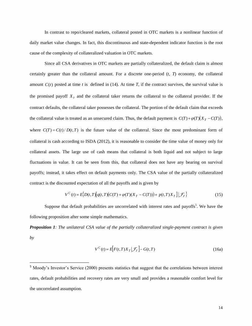
payoffs; instead, it takes effect on default payments only. The CSA value of the partially collateralized

contract is the discounted expectation of all the payoffs and is given by

tFTTC XTtpTCXTTCTtqTtDEtV ),())()(()(),(),()( (15)

Suppose that default probabilities are uncorrelated with interest rates and payoffs5. We have the

following proposition after some simple mathematics.

Proposition 1: The unilateral CSA value of the partially collateralized single-payment contract is given

by

),(),()( TtGXTtFEtV TC tF (16a)

5 Moody’s Investor’s Service (2000) presents statistics that suggest that the correlations between interest

rates, default probabilities and recovery rates are very small and provides a reasonable comfort level for

the uncorrelated assumption.

15

where

),(),(),(/11),()()()()(

TtDTtITtITtFtHtVtHtV NN

(16b)

),(/)(1),()(1),()()(

TtITTtqtHTtGtHtV N

(16c)

where tF),(),( TtIETtI . ),( TtI and )(tV N are defined in (9).

Proof: See the Appendix.

We may think of ),( TtF as the unilaterally CSA-adjusted discount factor and ),( TtG as the cost

of bearing unsecured credit risk. Proposition 1 tells us that the value of the unilaterally collateralized

contract is equal to the present value of the payoff discounted by the unilaterally CSA-adjusted discount

factors minus the cost of taking unsecured counterparty risk.

The valuation in equation (16) is relatively straightforward. We first compute )(tV N and then test

whether its value is greater than )(tH . After that, the calculations of ),( TtF , ),( TtG and )(tV C are

easily obtained.

We discuss the following two cases. Case 1: 0)( tH corresponds to full-collateralization. We

have )()( tVtV FC according to (16) where 0)( tH and 0)( tV N . That is to say: the CSA value under

full-collateralization is equal to the risk-free value, which is in line with the results of Johannes and

Sundaresan (2007), Fuijii and Takahahsi (2012), and Piterbarg (2010). Due to the mathematical

tractability and simplicity, previous modeling works focus on full-collateralization only. As we point out

above, however, full-collateralization does not appear to exist in any markets.

Case 2: 0)( tH represents partial-collateralization. Equation (16) yields )()()( tVtVtV FCN

when 0H . In particular, )()( tVtV CN when H . Therefore, we conclude that the CSA value

under partial-collateralization is less than the risk-free value but greater than the non-CSA value. Partial-

collateralization that reflects the risk tolerance and commercial intent of firms is mostly seen in OTC

markets.

16

Proposition 1 can be easily extended from one-period to multiple-periods. Suppose that a

defaultable portfolio/contract has m netted cash flows. Let the m cash flows be represented as 0iX

with payment dates iT , where i = 1,…,m. We derive the following proposition:

Proposition 2: The unilateral CSA value of the partially collateralized multiple-payment contract is given

by

1

0 1

1

0 11

1

0 1 ),(),(),()(m

i ii

i

j jj

m

i i

i

j jjC TTGTTFEXTTFEtV tt FF (17a)

where

),(),(),(/11),( 111)(),()(),(1 11 jjjjjjTHTTJTHTTJjj TTDTTITTITTF

jjjjjj (17b)

),(/)(1),()(1),( 111)(),(1 1 jjjjjjTHTTJjj TTITTTqTHTTG

jjj (17c)

jTF11111 )(),(),(),( jj

C

jjjjjj XTVTTITTDETTJ (17d)

Proof: See the Appendix.

The valuation in Proposition 2 has a backward nature. The intermediate values are vital to

determine the final price. For a payment period, the current price has a dependence on the future price.

Only on the final payment date mT , the value of the contract and the maximum amount of information

needed to determine the ),( 1 mm TTJ , ),( 1 mm TTF and ),( 1 mm TTG are revealed. This type of problem can

be best solved by working backward in time, with the later value feeding into the earlier ones, so that the

process builds on itself in a recursive fashion, which is referred to as backward induction. The most

popular backward induction valuation algorithms are lattice/tree and regression-based Monte Carlo.

3. Bilateral Collateralization

A bilateral collateral arrangement enables the counterparties to pass collateral between each other

to cover the net MTM exposure of the contracts. Under a two-way arrangement, the collateralization

17

obligation is mutual and applicable to both the client and dealer. Bilateral collateralization most likely

appears in OTC markets.

Two counterparties are denoted as A and B. The binomial default rule considers only two possible

states: default or survival. Therefore, the default indicator jY for party j (j=A, B) follows a Bernoulli

distribution, which takes value 1 with default probability jq and value 0 with survival probability jp , i.e.,

jj pYP }0{ and jj qYP }1{ . The marginal default distributions can be determined by the reduced-

form models. The joint distributions of a bivariate Bernoulli variable can be easily obtained via the

marginal distributions by introducing extra correlations.

Consider a pair of random variables ( AY , BY ) that has a bivariate Bernoulli distribution. The joint

probability representations are given by

ABBABA ppYYPp )0,0(:00 (18a)

ABBABA qpYYPp )1,0(:01 (18b)

ABBABA pqYYPp )0,1(:10 (18c)

ABBABA qqYYPp )1,1(:11 (18d)

where jj qYE )( ,

jjj qp2 , BBAAABBAABBBAAAB pqpqqYqYE ))((: where AB denotes

the default correlation coefficient and AB denotes the default covariance.

For a two-way CSA, each party has an effective collateral threshold and is required to post

collateral to the other as exposures arise. The collateral amount at t is given by

AC

AC

BC

A

BC

BC

HtVifHtV

HtVHif

HtVifHtV

tC

)()(

)(0

)()(

)( (19a)

or

AC

HtVBC

HtV HtVHtVtCAB

)(1)(1)( )()( (19b)

18

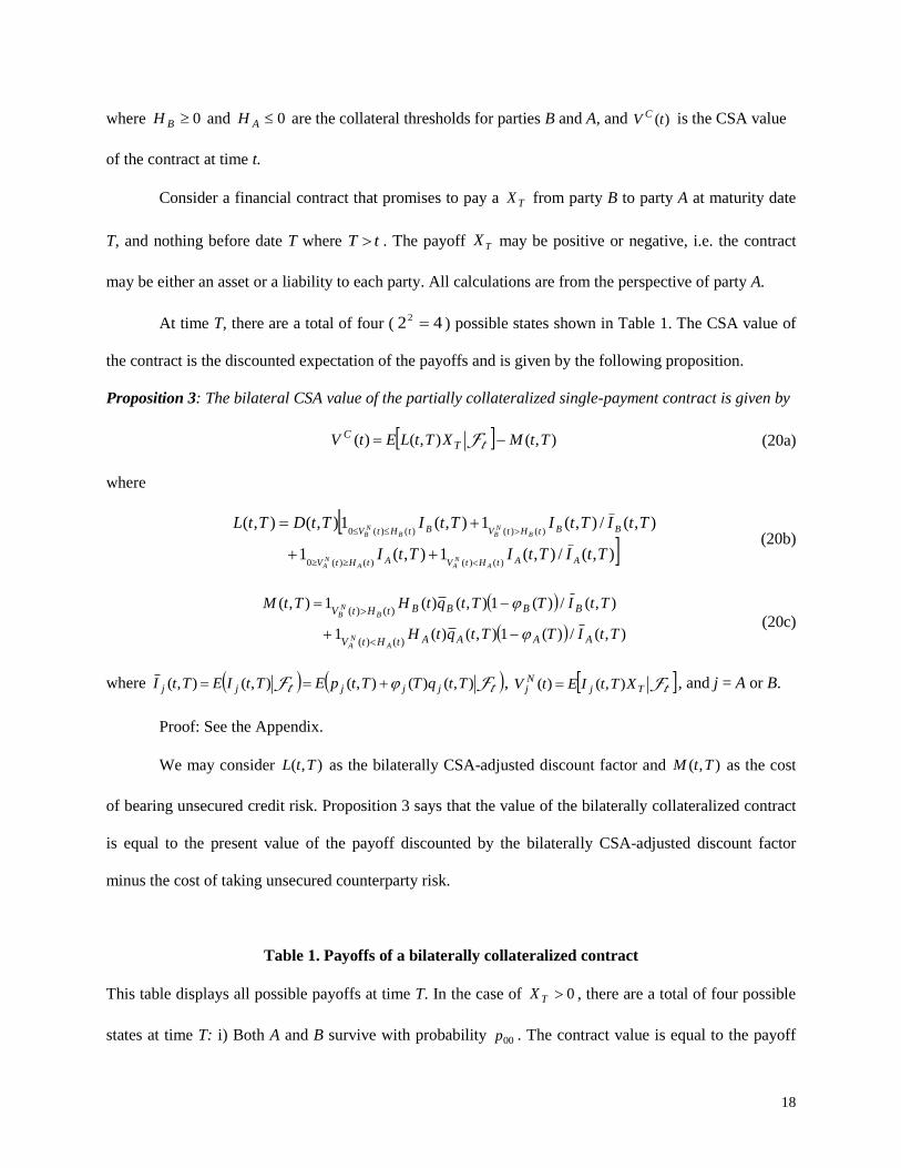
where 0BH and 0AH are the collateral thresholds for parties B and A, and )(tV C is the CSA value

of the contract at time t.

Consider a financial contract that promises to pay a TX from party B to party A at maturity date

T, and nothing before date T where tT . The payoff TX may be positive or negative, i.e. the contract

may be either an asset or a liability to each party. All calculations are from the perspective of party A.

At time T, there are a total of four ( 422 ) possible states shown in Table 1. The CSA value of

the contract is the discounted expectation of the payoffs and is given by the following proposition.

Proposition 3: The bilateral CSA value of the partially collateralized single-payment contract is given by

),(),()( TtMXTtLEtV TC tF (20a)

where

),(/),(1),(1

),(/),(1),(1),(),(

)()()()(0

)()()()(0

TtITtITtI

TtITtITtITtDTtL

AAtHtVAtHtV

BBtHtVBtHtV

AN

AAN

A

BN

BBN

B

(20b)

),(/)(1),()(1

),(/)(1),()(1),(

)()(

)()(

TtITTtqtH

TtITTtqtHTtM

AAAAtHtV

BBBBtHtV

AN

A

BN

B

(20c)

where tt FF ),()(),(),(),( TtqTTtpETtIETtI jjjjj , tFTjNj XTtIEtV ),()( , and j = A or B.

Proof: See the Appendix.

We may consider ),( TtL as the bilaterally CSA-adjusted discount factor and ),( TtM as the cost

of bearing unsecured credit risk. Proposition 3 says that the value of the bilaterally collateralized contract

is equal to the present value of the payoff discounted by the bilaterally CSA-adjusted discount factor

minus the cost of taking unsecured counterparty risk.

Table 1. Payoffs of a bilaterally collateralized contract

This table displays all possible payoffs at time T. In the case of 0TX , there are a total of four possible

states at time T: i) Both A and B survive with probability 00p . The contract value is equal to the payoff

19

TX . ii) A defaults but B survives with probability 10p . The contract value is also the payoff TX . Here we

follow the two-way payment rule6. iii) A survives but B defaults with probability 01p . The contract value

is the collateralized default payment: )()()( TCXTTC TB . iv) Both A and B default with probability

11p . The contract value is also )()()( TCXTTC TB . A similar logic applies to the case of 0TX .

State 0,0 BA YY 0,1 BA YY 1,0 BA YY 1,1 BA YY

Comments A & B survive A defaults, B survives A survives, B defaults A & B default

Probability 00p 10p

01p 11p

Payoff

0TX TX TX )()()( TCXTTC TB )()()( TCXTTC TB

0TX TX ))()(()( TCXTTC TA TX )()()( TCXTTC TA

In particular, if 0 BA HH (corresponding to bilateral full-collateralization), and ),( TtI i and

TX are uncorrelated, we have 1),( TtL , 0),( TtM , and thereby )()( tVtV FC . That is to say, under

full-collateralization the bilateral CSA value of the contract is equal to the risk-free value.

Using a similar derivation as in Proposition 2, we can easily extend Proposition 3 from one-

period to multiple-periods. Suppose that a defaultable portfolio/contract has m netted cash flows. Let the

m cash flows be represented as iX with payment dates iT , where i = 1,…,m. Each cash flow may be

positive or negative. The bilateral CSA value of the multiple payment contract is given by

1

0 1

1

0 11

1

0 1 ),(),(),()(m

i ii

i

k kk

m

i i

i

k kkC TTMTTLEXTTLEtV tt FF (21a)

6 There are two default settlement rules in the market. The one-way payment rule was specified by the

early ISDA master agreement. The non-defaulting party is not obligated to compensate the defaulting

party if the remaining market value of the instrument is positive for the defaulting party. The two-way

payment rule is based on current ISDA documentation. The non-defaulting party will pay the full market

value of the instrument to the defaulting party if the contract has positive value to the defaulting party.

20

where

),(/),(1),(1

),(/),(1),(1),(),(

11)(),(1)(),(0

11)(),(1)(),(011

11

11

kkAkkATHTTOkkATHTTO

kkBkkBTHTTOkkBTHTTOkkkk

TTITTITTI

TTITTITTITTDTTL

kAkkAkAkkA

kBkkBkBkkB (21b)

),(/)(1),()(1

),(/)(1),()(1),(

111)(),(

111)(),(1

1

1

kkBkAkkAkATHTTO

kkBkBkkBkBTHTTOkk

TTITTTqTH

TTITTTqTHTTM

kAkkA

kBkkB

(21c)

where kTkk

C

kkBkkkkj XTVTTITTDETTO F11111 )(),(),(),( and j = A or B.

Similar to Proposition 2, the individual payoffs in equation (21) are coupled and cannot be

evaluated separately. The process requires a backward induction valuation.

4. Empirical Results

The objective of this paper is to assess the economic significance and implications of

collateralization, which is essentially a matter of theoretical justification and empirical verification. We

choose interest rate swaps for our empirical study, as they are the largest component of the global OTC

derivative market, collectively accounting for around two-thirds of both the notional and market value of

all outstanding derivatives.

Swap rate is the fixed rate that sets the market value of a given swap at initiation to zero. ISDA

established ISDAFIX in 1998 in cooperation with Reuters (now Thomson Reuters) and Intercapital

Brokers (now ICAP PLC). Each day ISDAFIX establishes average mid-market swap rates at key terms to

maturity. These generic benchmark swap rates are based on a rigorously organized daily poll: An ICAP or

Reuters representative canvasses a panel of dealers for their par swap rate quotes as of a specified local

mid-day time. For any given swap term to maturity, the rate provided by the contributing dealer is the

midpoint of where that dealer would itself offer and bid a swap for a certain notional. The mid-market

benchmark rate for any given swap tenor is determined as a trimmed mean. Reuters and Bloomberg post

the mid-market rates as soon as polling is completed.

21

In practice, the mid-market swap rates are generally not the actual swap rates transacted with

counterparties, but are instead the benchmarks against which the actual swap rates are set. A swap dealer

that arranges a contract and provides liquidity to the market involves costs, e.g., hedging cost, credit cost,

liquidity cost, operational cost, tax cost, and economic capital cost, etc. Therefore, it is necessary to adjust

the mid-market swap rate to cover various costs of transacting and also to provide a profit margin to the

dealer that makes the market. As a result, the actual price agreed for the transaction is not zero but a

positive amount to the dealer.

Unlike the generic benchmark swap rates, swap premia are determined according to the basic

principles of supply and demand. The swap market is highly competitive. In a competitive market, prices

are determined by the impersonal forces of demand and supply, but not by manipulations of powerful

buyers or sellers. If a premium is set too low, the dealer may lose money. If the premium is set too high,

the dealer may lose the competitive advantage.

In contrast to most previous studies that focus on the generic swap rates, this article mainly

studies swap adjustments/premia related to credit risk and collateralization. It empirically measures the

effect of collateralization on pricing and compares it with model-implied prices.

A swap premium is supposed to cover the expected profit and all the expenses, including the cost

of bearing unsecured credit risk. Unfortunately, however, we do not know what percentage of the market

swap premium is allocated to the unsecured credit risk, which makes a direct verification impossible.

To circumvent this difficulty, we design an indirect verification process in which we select some

CSA swap pairs, where the two contracts in each pair have exactly the same terms and conditions but are

traded with different counterparties under different collateral agreements. It is reasonable to believe that

the only difference between the two contracts in each pair is the difference in unsecured credit risk

between two counterparties, as all other risks and costs are identical. Therefore, by taking credit risk and

collateralization into account only, we can compare the model-implied swap premium spreads with the

market swap premium spreads for these pairs.

22

We obtain a unique proprietary data set from an investment bank (FinPricing (2018)). The data

set contains swap contract data, counterparty data (including collateral agreements, recovery rates, etc),

and market data. The trading dates are from May 6, 2005 to May 11, 2012. The data show that before

2011 the dealer traded interest rate swaps with a large number of counterparties. But sine 2011, the

transactions have been concentrated in a few clearinghouses, which reflect financial institutions’

compliance with the regulatory requirements. Consequently, we divide the data into two categories: the

OTC data set containing all the transactions traded with regular counterparties and the cleared data set

holding all the contracts cleared in CCPs.

Let us examine the OTC data first. We find a total of 1002 swap pairs in the OTC data set, where

the two contracts in each pair have the same terms and conditions but are traded with different

counterparties under different collateral arrangements. We arbitrarily select one pair shown in Table 2.

Table 2: A pair of 20-year swap contracts

This table displays the terms and conditions of two swap contracts. They have different counterparties but

are otherwise the same. We hide the counterparty names according to the security policy of the

investment bank while everything else is authentic.

Swap 1 Swap 2

Fixed leg Floating leg Fixed leg Floating leg

Counterparty X Y

Effective date 15/09/2005 15/09/2005 15/09/2005 15/09/2005

Maturity date 15/09/2025 15/09/2025 15/09/2025 15/09/2025

Day count 30/360 ACT/360 30/360 ACT/360

Payment frequency Semi-annually Quarterly Semi-annually Quarterly

Swap rate 4.9042% - 4.9053% -

Roll over Mod_follow Mod_follow Mod_follow Mod_follow

Principal 25,000,000.00 25,000,000.00 25,000,000.00 25,000,000.00

23

Currency USD USD USD USD

Pay/receive Bank receives Party X receives Bank receives Party Y receives

Floating index - 3 month LIBOR - 3 month LIBOR

Floating spread - 0 - 0

Floating reset - Quarterly - Quarterly

An interest rate curve is the term structure of interest rates, derived from observed market

instruments that represent the most liquid and dominant interest rate products for certain time horizons.

Normally the curve is divided into three parts. The short end of the term structure is determined using the

LIBOR rates. The middle part of the curve is constructed using Eurodollar futures that require convexity

adjustments. The far end is derived using mid swap rates. The LIBOR-future-swap curve is presented in

Table 3. After bootstrapping the curve, we get the continuously compounded zero rates.

Table 3: USD LIBOR-future-swap curve

This table displays the closing mid prices as of September 15, 2005

Instrument Name Price

September 21 2005 LIBOR 3.6067%

September 2005 Eurodollar 3 month 96.1050

December 2005 Eurodollar 3 month 95.9100

March 2006 Eurodollar 3 month 95.8100

June 2006 Eurodollar 3 month 95.7500

September 2006 Eurodollar 3 month 95.7150

December 2006 Eurodollar 3 month 95.6800

2 year swap rate 4.2778%

3 year swap rate 4.3327%

4 year swap rate 4.3770%

5 year swap rate 4.4213%

24

6 year swap rate 4.4679%

7 year swap rate 4.5120%

8 year swap rate 4.5561%

9 year swap rate 4.5952%

10 year swap rate 4.6368%

12 year swap rate 4.7089%

15 year swap rate 4.7957%

20 year swap rate 4.8771%

25 year swap rate 4.9135%

As the payoff of an interest rate swap is determined by interest rates, we need to model the

evolution of the floating rates. Interest rate models are based on evolving either short rates, instantaneous

forward rates, or market forward rates (e.g., the LIBOR Market Model (LMM)). Since both short rates

and instantaneous forward rates are not directly observable in the market, the models based on these rates

have difficulties in expressing market views and quotes in term of model parameters, and lack agreement

with market valuation formulas for basic derivatives. On the other hand, the object modeled under the

LMM is market-observable. It is also consistent with the market standard approach for pricing caps/floors

using Black’s formula. They are generally considered to have more desirable theoretical calibration

properties than short rate or instantaneous forward rate models. Therefore, we choose the LMM lattice

proposed by Xiao (2011) for pricing collateralized swaps. We also implement the Hull-White trinomial

tree to verify the results and ensure robustness of the valuation. This paper, however, only reports the

results produced by the LMM lattice.

According to equation (21), we also need counterparty-related information, such as recovery rates,

hazard rates and collateral thresholds. The CDS spreads and recovery rates are given in Table 4. We can

compute the hazard rates via a standard calibration process (see J.P. Morgan [2001]).

25

Table 4: CDS premia and recovery rates

This table displays the closing CDS premia as of September 15, 2005 and recovery rates

Counterparty name Bank Company X Company Y

6 month CDS spread 0.00031 0.000489 0.000808

1 year CDS spread 0.000333 0.00056 0.001017

2 year CDS spread 0.000516 0.000866 0.00154

3 year CDS spread 0.000664 0.001147 0.002114

4 year CDS spread 0.000848 0.00147 0.002768

5 year CDS spread 0.001012 0.001783 0.003439

7 year CDS spread 0.001334 0.002289 0.004283

10 year CDS spread 0.001727 0.002952 0.005281

15 year CDS spread 0.001907 0.003283 0.005814

20 year CDS spread 0.002023 0.003266 0.006064

30 year CDS spread 0.002021 0.00336 0.006461

Recovery rate 0.39213 0.35847 0.33872

Table 5: CSA agreement

This table provides the collateral thresholds and MTAs under the CSA agreements.

CSA agreement 1 2

Counterparty name Bank Company X Bank Company Y

Threshold 0 0 0 0

MTA 500000 500000 500000 500000

The collateral thresholds and MTAs of the CSA agreements are displayed in Table 5. The

effective collateral threshold is equal to the threshold plus the MTA.

Given the above information, we are able to compute the collateralized swap rates. We first use

the LMM to evolve the interest rates and then determine the associated CSA-adjusted discount factors as

26

well as the cost of bearing unsecured credit risk according to equation (21). Finally, we calculate the

collateralized swap rates via backward induction method. The results are given in table 6.

Table 6: Swap rate results

This table presents the model-implied swap rates and premia as well as the dealer-quoted swap rates and

premia, where Swap premium (in bps) = Swap rate – Generic swap rate, and Premium spread = Premium

of swap 2 – Premium of swap 1.

Swap 1 Swap 2

Premium spread

Generic

swap rate Swap rate Premium Swap rate Premium

Model-implied 0.048780 0.09 bps 0.048790 0.19 bps 0.10 bps

0.048771

Dealer quoted 0.049042 2.71 bps 0.049053 2.82 bps 0.11 bps

The 20-year generic mid-market swap rate is 0.048771 shown in Table 3. The swap rates of

contracts 1 and 2 are given in Table 2 as 0.049042 and 0.049053. Accordingly, the market swap premia

are 2.71 (0.049042 - 0.048771) basis points (bps) and 2.82 bps, respectively. These premia are charged

for many expenses, e.g., operational, liquidity, funding, credit, etc., as well as profit margins. Although

we do not know what percentage of the premia are allocated to cover the unsecured credit risks, we

reasonably believe that the market premium spread, 0.11 bps in Table 6, should reflect the difference

between the counterparties’ unsecured credit risks only, as other factors are identical.

By taking credit risk and collateralization into account only, we calculate the model-implied swap

rates as 0.048780 and 0.048790 shown in Table 6. Consequently, the implied swap premia are 0.09 bps

and 0.19 bps. The results imply that only a small portion of a swap premium is attributed to unsecured

credit risk. This is in line with the findings of Duffie and Huang (1996), Duffie and Singleton (1997), and

Minton (1997). Table 6 shows that the model-implied swap premium spread is quite close to the dealer-

quoted swap premium spread, suggesting that the model is fairly accurate in pricing collateralized

financial instruments.

27

Repeating this exercise for the remaining pairs, we find that the model-implied swap premia

fluctuate randomly around the market swap premia. The summary statistics of the market quoted

premium spreads, the model-implied premium spreads, and the model-market premium spread

differentials are presented in Table 7, where we refer to the differences between the model-implied

premium spreads and the market quoted premium spreads as the model-market premium spread

differentials. As can be seen from Table 7, the average of the model-market spread differentials is only -

0.03 bps, which can be partly attributed to noises. The results indicate prima facie that the model performs

quite well. The empirical tests corroborate the theoretical prediction on the impact of collateralization on

swap rates.

Table 7: Summary statistics of implied swap premium spreads, market swap premium spreads and

model-market swap premium spread differentials

All values are displayed in bps. Model-market premium spread differential = Model-implied premium

spread – Market-quoted premium spread.

Max Min Mean Median Std

Market quoted swap premium spreads 3.08 -5.25 -0.46 -0.15 1.80

Model-implied swap premium spreads 2.10 -5.33 -0.44 0.03 1.73

Model-market premium spread differentials 0.99 -1.18 -0.03 0.11 0.46

Next, we examine the effects of credit risk and collateralization, alone or combined, on swap

premium spreads. First, we study the marginal effect of credit risk. For each swap pair, we calculate the

difference between the CDS spreads of the two counterparties. Presumably, differences in CDS spreads

should mainly represent differences in pure credit risk. To determine the strength of the statistical

relationship between market swap premium spreads and differences between associated CDS spreads, we

present the estimate of the following regression model.

bXaY (22)

28

where Y is the market swap premium spread, X is the difference between the CDS spreads, a is the

intercept, b is the slope, and is the regression residual.

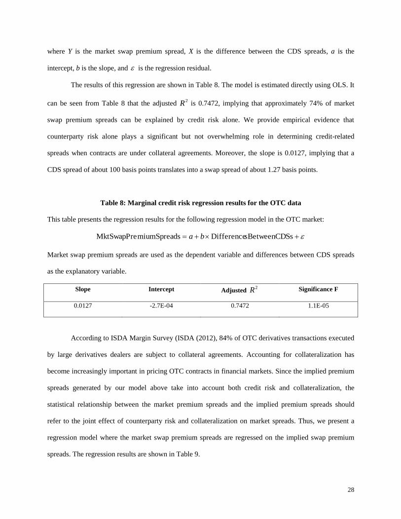
The results of this regression are shown in Table 8. The model is estimated directly using OLS. It

can be seen from Table 8 that the adjusted 2R is 0.7472, implying that approximately 74% of market

swap premium spreads can be explained by credit risk alone. We provide empirical evidence that

counterparty risk alone plays a significant but not overwhelming role in determining credit-related

spreads when contracts are under collateral agreements. Moreover, the slope is 0.0127, implying that a

CDS spread of about 100 basis points translates into a swap spread of about 1.27 basis points.

Table 8: Marginal credit risk regression results for the OTC data

This table presents the regression results for the following regression model in the OTC market:

SssBetweenCDDifferencesmiumSpreadMktSwapPre ba

Market swap premium spreads are used as the dependent variable and differences between CDS spreads

as the explanatory variable.

Slope Intercept Adjusted 2R Significance F

0.0127 -2.7E-04 0.7472 1.1E-05

According to ISDA Margin Survey (ISDA (2012), 84% of OTC derivatives transactions executed

by large derivatives dealers are subject to collateral agreements. Accounting for collateralization has

become increasingly important in pricing OTC contracts in financial markets. Since the implied premium

spreads generated by our model above take into account both credit risk and collateralization, the

statistical relationship between the market premium spreads and the implied premium spreads should

refer to the joint effect of counterparty risk and collateralization on market spreads. Thus, we present a

regression model where the market swap premium spreads are regressed on the implied swap premium

spreads. The regression results are shown in Table 9.

29

It can be seen from Table 9 that the implied premium spreads explicate nearly all of the market

premium spreads with a slope coefficient close to 1. More important, the adjusted 2R value is 0.9565,

implying that approximately 96% of the market premium spreads can be explained by the implied spreads.

The empirical results shed light on the economic significance of collateralization. We find evidence that

credit risk is not overly important in spreads. Only the combination of credit risk and collateralization can

provide a sufficient explanation for these price differences.

Table 9: Credit risk and collateralization combined regression results for the OTC data

This table presents the regression results for the following regression model in the OTC market:

readspPremiumSpImpliedSwasmiumSpreadMktSwapPre ba

The market swap premium spreads are used as a dependent variable and the implied swap premium

spreads as the explanatory variable.

Slope Intercept Adjusted 2R Significance F

0.9857 4.48E-05 0.9565 3.21E-08

Finally, we turn to cleared markets. We have found a total of 403 swap pairs in the cleared data

set, where the two contracts in each pair have the same terms and conditions. The statistics of market-

quoted swap premium spreads for both the OTC data set and the cleared data set are presented in Table 10.

It is shown from the table that swap premium spreads in cleared markets behave in the same way as those

in OTC markets, i.e., market swap premium spreads in both cleared markets and OTC markets are

statistical similar.

We empirically demonstrate that under the new regulatory rules, derivative are continuously

negotiated over-the-counter as usual, and then cleared and settled through a clearinghouse. Since

clearinghouses claim that cleared derivatives would replicate OTC derivatives and promise that

30

transactions through the clearinghouses would be economically equivalent to similar transactions handled

in OTC markets, swap rates in cleared markets are determined in the same way as those in OTC markets.

Table 10: Statistics of market observed swap premium spreads

This table presents descriptive statistics for market swap premium spreads in both OTC and cleared

markets. All values are expressed in bps.

Market quoted swap premium spreads Max Min Mean Median Std

In the OTC data set 3.08 -5.25 -0.46 -0.15 1.80

In the cleared data set 3.51 -4.41 -0.34 -0.21 1.27

Many market participants, however, have cast doubt on the claim of economic equivalence. They

find that cleared contracts have actually significant differences when compared with OTC trades. Some

firms even file legal action against the clearinghouses, and accuse them of fraudulently inducing the firms

to enter into cleared derivatives on the premise the contracts would be economically equivalent to OTC

contracts (see Pengelly (2011)).

There are many reasons to question this practice. First, the results generated by this practice can

not be interpreted by any known models or theories. As clearinghouses hide counterparties, we can only

see the clearinghouses in the data. The two contracts in each cleared swap pair have exactly the same

counterparty (i.e., the same CCP) and terms and conditions but different swap rates. In other words, they

appear to be identical in everything except swap rates. This violates the single value rule: two assets with

identical information must be traded at the same price.

Since the clearinghouse is the counterparty in all transactions, counterparty credit risk is

always the same for a dealer. Consequently, the prices of individual transactions should not be

influenced by difference in counterparty credit risk, i.e., swap premium spreads should be zero in

cleared markets. Said differently, the presence of swap premium spreads in cleared markets goes

against the conventional wisdom and can not be explained theoretically and intuitively.

31

Second, there are many differences between cleared markets and OTC markets. The first

difference is that cleared derivatives are over-collateralized as all CCPs require initial margins, whereas

CSA derivatives in OTC markets are partially collateralized as all CSA counterparties maintain a positive

MTA. The second difference is that cleared derivatives are subject to unilateral collateralization because

only CCPs have the right to call for collateral, while OTC derivatives are most probably under bilateral

collateralization. The third difference is that OTC collateral agreements always set a MTA to avoid the

workload associated with a frequent transfer of insignificant amount of collateral between firms, whilst

CCPs mark contracts to market daily and charge variation margins in response to changes in market

values without a MTA.

The fourth difference is that variation margin in clearing markets is a linear function of daily

market value changes. Whereas, collateral posted in OTC markets is a nonlinear function of daily market

value changes. When the MTM value is greater than the threshold and the daily value change exceeds the

MTA, collateral is called; otherwise, no transfer of collateral occurs. This non-linearity is the root cause

of the complexity of pricing collateralized OTC derivatives.

The fifth difference is that a CCP mitigates credit risk via novation and multilateral netting. The

novation process splits a contract into two – one setting out a sale and the other setting out the

countervailing purchase – and substitutes the clearinghouse for the counterparty in each half of the

transaction. Accordingly, the clearinghouse takes on credit risk on behalf of the original counterparties.

The multilateral netting process enables offsets across market participants, which further ameliorates

credit risk (see Cont and Kokholm (2011) and McPartland, et al. (2011)). In general, novation and

multilateral netting processes change the risk structure that affects asset prices.

The last difference is that in cleared markets, a party receiving variation margin owns the funds

and may withdraw them from the clearinghouse, while in OTC markets, a party posting collateral

maintains ownership of the assets and receives interest (or coupons) on the assets. Many CCPs use the

price alignment interest (PAI) adjustment or similar – a daily cash payment – to correct the difference in

32

interest on variation margin between OTC contracts and CCP products (see Cont, Mondescu and Yu

(2011)).

Even trivial variations between cleared and OTC markets can result in potentially large valuation

discrepancy (see Pengelly (2011)). Given many differences between them, our theoretical study shows

that over-collateralized derivatives in cleared markets are not economically equivalent to their partially

collateralized counterparts in OTC markets.

Clearinghouses stand ready to act as counterparties to transactions with other market participants.

The business of a clearinghouse closely resembles that of a specialized (monocline) insurer. Thus, the

clearinghouse makes money in a similar way too – by charging fees to its members. For example, LCH

Swap Clear does not levy a charge per transaction but instead charges its members an annual fee

depending on their level of usage. Clearing members then pass on those charges to clients as part of their

fee structure.

From a dealer’s perspective, market making involves costs and executing a transaction in a

clearinghouse also entails expenses. Dealers that make markets must be compensated for incurring these

costs and expanses. As a consequence, dealers in cleared markets also collect a swap premium for a

transaction. However, swap premia charged in cleared markets should be different from those collected in

OTC markets, as cost and risk structures have changed. At least, if two contracts have exactly the same

terms and conditions as well as the same counterparty (i.e., the clearinghouse), they should have the same

premia, as the swap premia should not be influenced by difference in counterparty credit risk in cleared

markets. The discussions above may have important implications for regulators, academics and

practitioners. A better understanding of collateralization would enable them to more accurately assess the

impact of new regulation on financial markets.

5. Conclusion

This article addresses a very important topic of the impact of collateralization on asset prices and

risk management. This is the so called plumbing of financial system that affects many outcomes.

33

We present a comprehensive theoretical framework for pricing collateralized financial contracts

based on the fundamental principal and legal structure of CSA agreements. The model can back out

differences in asset prices due to collateralized counterparty risk. This is very useful for pricing

outstanding defaultable financial contracts.

Empirically, we use a unique proprietary data set to measure the effect of collateralization on

pricing and compare it with model-implied prices. We find a quite number of swap contracts that have

different collateral arrangements but are similar otherwise. Presumably, differences in swap rates should

be largely attributable to differences in counterparty risk. The empirical results show that model-implied

prices are quite close to market-quoted prices, which suggests the model is fairly accurate in pricing

collateralized contracts.

We find strong evidence that counterparty risk alone plays a significant but not overwhelming

role in determining credit-related spreads for collateralized contracts. Only the joint effect of

collateralization and credit risk can provide a sufficient explanation for unsecured credit costs. This

finding suggests that failure to properly account for collateralization may result in significant mispricing

of financial contracts.

We also find evidence that financial institutions are sprinting to comply with the Dodd-Frank Act.

In the new practice, contracts are continuously negotiated over-the-counter as usual, but cleared and

settled via clearinghouses, as clearinghouses claim that cleared contracts would be economically

equivalent to their OTC counterparts. As a result, swap premia in cleared market are determined in a

similar way to those in OTC markets. We argue that this practice may not be appropriate because we

notice that the clearing mechanics of a clearinghouse change the risk structure and thereby the asset prices.

In fact, we find that cleared derivatives are not economically equivalent to their OTC counterparts.

Appendix

34

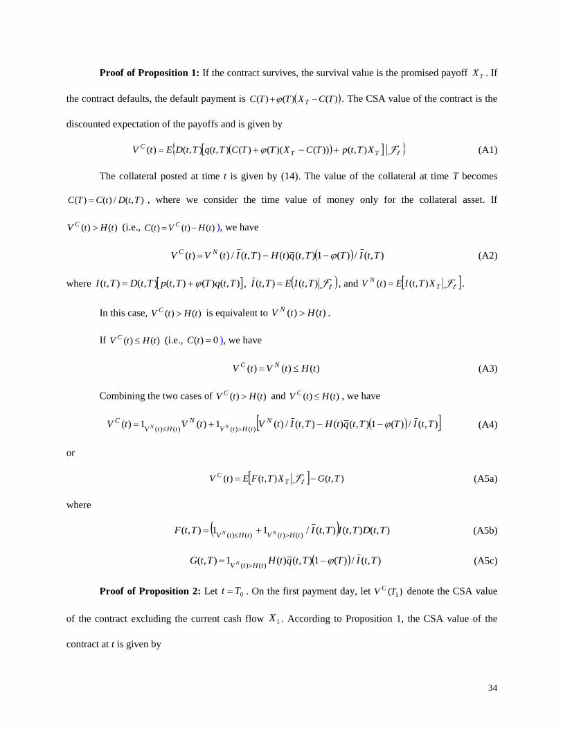
Proof of Proposition 1: If the contract survives, the survival value is the promised payoff TX . If

the contract defaults, the default payment is )()()( TCXTTC T . The CSA value of the contract is the

discounted expectation of the payoffs and is given by

tFTTC XTtpTCXTTCTtqTtDEtV ),())()(()(),(),()( (A1)

The collateral posted at time t is given by (14). The value of the collateral at time T becomes

),(/)()( TtDtCTC , where we consider the time value of money only for the collateral asset. If

)()( tHtV C (i.e., )()()( tHtVtC C ), we have

),(/)(1),()(),(/)()( TtITTtqtHTtItVtV NC (A2)

where ),()(),(),(),( TtqTTtpTtDTtI , tF),(),( TtIETtI , and tFTN XTtIEtV ),()( .

In this case, )()( tHtV C is equivalent to )()( tHtV N .

If )()( tHtV C (i.e., 0)( tC ), we have

)()()( tHtVtV NC (A3)

Combining the two cases of )()( tHtV C and )()( tHtV C , we have

),(/)(1),()(),(/)(1)(1)()()()()(

TtITTtqtHTtItVtVtV N

tHtV

N

tHtV

CNN

(A4)

or

),(),()( TtGXTtFEtV TC tF (A5a)

where

),(),(),(/11),()()()()(

TtDTtITtITtFtHtVtHtV NN

(A5b)

),(/)(1),()(1),()()(

TtITTtqtHTtGtHtV N

(A5c)

Proof of Proposition 2: Let 0Tt . On the first payment day, let )( 1TV C denote the CSA value

of the contract excluding the current cash flow 1X . According to Proposition 1, the CSA value of the

contract at t is given by

35

),()(),()( 101110 TTGTVXTTFEtV CC tF (A6)

Similarly, we have

),()(),()( 2122211 1TTGTVXTTFETV T

CC F (A7)

Note that ),( 10 TTG is 1TF -measurable. According to the taking out what is known and tower

properties of conditional expectation, we have

1

0 1

1

0 1

2

1

0 1

2

1

1

0 1

101110

),(),(

)(),(),(

),()(),()(

i ii

i

j jj

C

j jji i

i

j jj

CC

TTGTTFE

TVTTFEXTTFE

TTGTVXTTFEtV

t

tt

t

F

FF

F

(A8)

By recursively deriving from 2T forward over mT , where mmC XTV )( , we have

1

0 1

1

0 11

1

0 1 ),(),(),()(m

i ii

i

j jj

m

i i

i

j jjC TTGTTFEXTTFEtV tt FF (A9)

Proof of Proposition 3: At time T, there are a total of four possible states shown in Table 1. The

joint distributions of A and B are given by (18) and the collateral amount posted at time t is given by (19).

Depending on whether the value is in the money or out of the money at T, we have the following

situations

Case 1: 0)()( tHtV BC . We have )()()( tHtVtC B

C and

t

t

F

F

),(/)(1)()()(),(),(),(

)()()(),(),(),(),(),()( 11011000

TtDTtHtVXTTtqXTtpTtDE

TCXTTCTtpTtpXTtpTtpTtDEtV

BC

TBBTB

TBTC

(A10a)

or

),(/)(1),()(),(/)()( TtITTtqtHTtItVtV BBBBBN

BC (A10b)

where tFTBN

B XTtIEtV ),()( . In this case, 0)()( tHtV BC is equivalent to )()( tHtV B

NB .

Case 2: )()(0 tHtV B

C . We have 0)( tC and

)()(),(),(),()( tVXTTtqTtpTtDEtV NBTBBB

C tF (A11)

In this case, )()(0 tHtV B

C is equivalent to )()(0 tHtV B

N

B

36

Case 3: 0)()( tHtV AC . We have )()()( tHtVtC A

C and

t

t

F

F

)(1)()(),(),(),(

)()()(),(),(),(),(),()( 11100100

TTCXTTtqXTtpTtDE

TCXTTCTtpTtpXTtpTtpTtDEtV

ATAATA

TATC

(A12a)

or

),(/)(1),()(),(/)()( TtITTtqtHTtItVtV AAAAAN

AC (A12b)

where tFTBN

B XTtIEtV ),()( . In this case, 0)()( tHtV AC is equivalent to )()( tHtV A

NA .

Case 4: )()(0 tHtV A

C . We have 0)( tC and

)()(),(),(),()( tVXTTtqTtpTtDEtV NATAAA

C tF (A13)

In this case, )()(0 tHtV AC is equivalent to )()(0 tHtV A

N

A .

Combining the four cases together, we have

),(),()( TtMXTtLEtV TC tF (A14a)

Where

),(/),(1),(1

),(/),(1),(1),(),(

)()()()(0

)()()()(0

TtITtITtI

TtITtITtITtDTtL

AAtHtVAtHtV

BBtHtVBtHtV

AN

AAN

A

BN

BBN

B

(A14b)

),(/)(1),()(1

),(/)(1),()(1),(

)()(

)()(

TtITTtqtH

TtITTtqtHTtM

AAAAtHtV

BBBBtHtV

AN

A

BN

B

(A14c)

where tt FF ),()(),(),(),( TtqTTtpETtIETtI jjjjj , tFTjNj XTtIEtV ),()( , and j = A or B.

References

AFME, ICMA, and ISDA, 2011, “The impact of derivative collateral policies of European sovereigns and

resulting Basel III capital issues.”

Collin-Dufresne, P. and B. Solnik, 2001, “On the term structure of default premia in the swap and LIBOR

markets,” Journal of Finance 56, 1095-1115.

37

Cont, R. and T. Kokholm, 2011, “Central clearing of OTC derivatives bilateral vs. multilateral netting,”

Working paper.

Cont, R., R. Mondescu, and Y. Yu, 2011, “Central clearing of interest rate swaps: a comparison of

offerings,” Working Paper.

Duffie, D. and M. Huang, 1996, “Swap rates and credit quality,” Journal of Finance, 51, 921-949.

Duffie, D., and K.J. Singleton, 1999, “Modeling term structure of defaultable bonds,” Review of

Financial Studies, 12, 687-720.

Duffie, D., and H. Zhu, 2011, “Does a central clearing counterparty reduce counterparty risk?” Review of

Asset Pricing Studies, 74-95.

Edwards, F. and E. Morrison, 2005, “Derivatives and the bankruptcy code: why the special treatment?”

Yale Journal on Regulation, 22, 101-133.

Feldhutter, P. and D. Lando, 2008, “Decomposing swap spreads,” Journal of Financial Economics,” 88

(2), 375-405.

FinPricing, 2018, Investment banking solution, https://finpricing.com/aboutus.html

European Central Bank (ECB), 2009, “Credit default swaps and counterparty risk.”

Fuijii, M. and A. Takahahsi, “Collateralized CDS and default dependence – Implications for the central

clearing,” Forthcoming, Journal of Credit Risk.

Garlson, D., 1991-1992, “Secured creditors and the eely character of bankruptcy valuations,” 41

American University Law Review, 63, 63-106.

Grinblatt, M., 2001, “An analytic solution for interest rate swap spreads,” Review of International

Finance, 2, 113-149.

38

He, H., 2001, “Modeling Term Structures of Swap Spreads,” working paper, Yale School of Management,

Yale University.

Heller, D. and N. Vause, 2012, “Collateral requirements for mandatory central clearing of over-the-

counter derivatives,” BIS Working Papers, No 373.

Hentschel, L. and C. W. Smith, Jr., 1997, “Risks in Derivatives Markets: Implications for the Insurance

Industry." Journal of Risk and Insurance, 64, 323-346.

Hull, J., 2010, “OTC derivatives and central clearing: can all transactions be cleared?” Financial Stability

Review, 14, 71-80.

ISDA, 2013, Product Descriptions and Frequently Asked Questions (1. Major derivative categories; 2.

How do cleared derivatives differ from OTC derivatives?), http://www.isda.org/educat/faqs.html

ISDA, 2012, “ISDA margin survey 2012.”

Johannes, M. and S. Sundaresan, 2007, “The impact of collateralization on swap rates,” Journal of

Finance, 62, 383-410.

J.P. Morgan, 2001, “Par credit default swap spread approximation from default probabilities.”

Liu, J., F. Longstaff, and R. Mandell, 2006, "The Market Price of Risk in Interest Rate Swaps: The Roles

of Default and Liquidity Risks," The Journal of Business, vol. 79, pages 2337-2360.

McPartland, J., P. Khorrami, R. Ranjan, and K. Wells, 2011, “An algorithm to estimate the total amount

of collateral required before and after financial reform initiatives in various, regulatory jurisdictions,”

Federal Reserve Bank of Chicago.

Minton, B., 1997, “An Empirical Examination of Basic Valuation Models for Plain Vanilla U.S. Interest

Rate Swaps." Journal of Financial Economics, 251-277.

Moody’s Investor’s Service, 2000, “Historical default rates of corporate bond issuers, 1920-99,”

39

O’Kane, D. and S. Turnbull, 2003, “Valuation of credit default swaps,” Fixed Income Quantitative Credit

Research, Lehman Brothers, QCR Quarterly, 2003 Q1/Q2, 1-19.

Pengelly, M., 2011, “Margin minutiae at issue in Jefferies v IDCG suit,” Risk magazine, 02 Nov 2011

Pirrong, C., 2011, “The economics of central clearing: theory and practice,” ISDA Discussion Papers

Series.

Piterbarg, V., 2010, “Funding beyond discounting: collateral agreements and derivatives pricing,” Risk

Magazine, 2010 (2), 97-102.

Routh, R. and M. Douglas, 2005, “Default interest payable to oversecured creditor subject to

reasonableness limitation,” ABF Journal, Vol. 4, No. 3.

Singh, M., 2010, “Collateral, netting and systemic risk in the OTC derivatives market,” IMF Working

Paper No. 10/99.

Sorensen, E. and T. Bollier, 1994, “Pricing swap default risk,” Financial Analysts Journal, 50, 23-33.

Xiao, T., 2011, “An efficient lattice algorithm for the LIBOR market model,” Journal of Derivatives, 19

(1): 25-40.