an architecture of a multi-model system for planning and scheduling

This article was downloaded by: [University of Auckland Library]On: 08 October 2014, At: 14:28Publisher: Taylor & FrancisInforma Ltd Registered in England and Wales Registered Number: 1072954 Registered office:Mortimer House, 37-41 Mortimer Street, London W1T 3JH, UK

International Journal of ComputerIntegrated ManufacturingPublication details, including instructions for authors and subscriptioninformation:http://www.tandfonline.com/loi/tcim20

An architecture of a multi-model system forplanning and schedulingA. Artiba & E. H. AghezzafPublished online: 08 Nov 2010.

To cite this article: A. Artiba & E. H. Aghezzaf (1997) An architecture of a multi-model system forplanning and scheduling, International Journal of Computer Integrated Manufacturing, 10:5, 380-393, DOI:10.1080/095119297131110

To link to this article: http://dx.doi.org/10.1080/095119297131110

PLEASE SCROLL DOWN FOR ARTICLE

Taylor & Francis makes every effort to ensure the accuracy of all the information (the“Content”) contained in the publications on our platform. However, Taylor & Francis, our agents,and our licensors make no representations or warranties whatsoever as to the accuracy,completeness, or suitability for any purpose of the Content. Any opinions and views expressedin this publication are the opinions and views of the authors, and are not the views of orendorsed by Taylor & Francis. The accuracy of the Content should not be relied upon andshould be independently verified with primary sources of information. Taylor and Francis shallnot be liable for any losses, actions, claims, proceedings, demands, costs, expenses, damages,and other liabilities whatsoever or howsoever caused arising directly or indirectly in connectionwith, in relation to or arising out of the use of the Content.

This article may be used for research, teaching, and private study purposes. Any substantialor systematic reproduction, redistribution, reselling, loan, sub-licensing, systematic supply, ordistribution in any form to anyone is expressly forbidden. Terms & Conditions of access and usecan be found at http://www.tandfonline.com/page/terms-and-conditions

http://www.tandfonline.com/loi/tcim20

http://www.tandfonline.com/action/showCitFormats?doi=10.1080/095119297131110

http://dx.doi.org/10.1080/095119297131110

http://www.tandfonline.com/page/terms-and-conditions

An architecture of a multi-model system forplanning and scheduling

A. ARTIBA and E. H. AGHEZZAF

Abstract. An architecture of a multi-model based system forproduction planning and scheduling is described. The multi-model system is de® ned as a system integrating expertsystems techniques, discrete event simulation, optimizationalgorithms and heuristics to support decision making forcomplex production planning and schedulingproblems. Theobject-oriented approach is used for data modelling. Thefunctional modules and their interconnection will bedescribed. The operational architecture is described andthe implementation phases of a speci® c application withthe proposed system are explained. A hybrid ¯ owshopplanning and scheduling problem using the multi-modelapproach is then presented.

1. Introduction

Industrial companies are increasing the degree ofautomation of their production shops. Consequentlythey need more and more sophisticated computer-based production management systems for thesecomplex manufacturing systems. These decision sup-port systems are helpful in planning and schedulingactivities.

The development of production schedules is anextremely important task in industry, although this isan area where a theoretical approach has not provideda general solution because the speci® c features ofpractical examples are both numerous and varied(Artiba and Tahon 1992). The Operations Research(OR) community has been working on productionscheduling for decades. In the 1980s, researchers inproduction scheduling were interested in Arti® cialIntelligence (AI) techniques. This interest is motivatedby an attempt to respond to: (1) the inadequacies ofexisting computer-based solutions in this area and theconsequent ine� ciencies that plague industry today,

and (2) the limited impact that results from the® elds of OR has had over the years in practical factoryoperations. In contrast to the ® eld of OR, AI-basedapproaches to production management and controlhave emphasized the development of solutions thatmatch the requirements, characteristics and con-straints of practical production management prob-lems (Smith 1992).

Real mutual bene® ts can result between AI and OR(O’Keefe 1985): The knowledge engineer can bene® tfrom the experience of OR in model building; expertsystems will use OR techniques. For the OR scientist,the expert system is another tool in the tool kit.Integration with other computing systems will lead toDSS (Decision Support System) able to draw on aknowledge base and to reason with the user’.

Muller et al. (1987) illustrate some similaritiesbetween OR and AI approaches and point out thatOR should take advantage of the new techniquesprovided by AI technology to tackle complex produc-tion scheduling problems. OR heuristics o� er theadvantage of providing optimal (or near optimal)solutions for well structured scheduling problems.The AI formalism allows one to capture all the detailsof real world constraints, it also represents and mani-pulates the human scheduler’s knowledge.

Kusiak (1987) proposed a tandem architecture:knowledge-based systems and optimization algorithms.This approach is powerful when the scheduling prob-lem to be solved complies to the stored optimizationalgorithms.

A framework combining simulation and expertsystems for production planning and control was pro-posed by Falster (1987); he highlighted the advantagesof combining these two approaches.

The heuristic problem solving frameworks that haveemerged from the ® eld of AI can be seen as comple-mentary to the analytic technique produced by OR.These frameworks can provide a basis for exploiting

0951-192X/97 $12.00 � 1997 Taylor & Francis Ltd

INT. J. COMPUTER INTEGRATED MANUFACTURING, 1997, VOL. 10, NO. 5, 380± 393

Authors: A. Artiba and E. H. Aghezzaf, FUCAM, ChausseÂ e de Binche, 151,B-7000 Mons, Belgium.

Dow

nloa

ded

by [

Uni

vers

ity o

f A

uckl

and

Lib

rary

] at

14:

28 0

8 O

ctob

er 2

014

knowledge of model assumptions, parameters, set-up,and applicability to: (1) make existing OR techniquesmore accessible and usable to an end user, or (2)opportunistically exploit a collection of analytic/heuristic procedures as appropriate during the plan-ning/scheduling process (Smith 1992).

Artiba et al. (1989) used expert systems and ORheuristics to generate feasible schedules in hybrid¯ owshop environments and proposed to generalizethis approach to a multi-model system. This systemcombines (but is not restricted to) OR and AI tech-niques and discrete event simulation (Artiba 1994a).

A knowledge-based scheduler which adopts thehierarchical approach and utilizes simulation tech-niques was developed by Doulgeri et al. (1993).

Kadaba et al. (1991) integrated the machine learn-ing process with knowledge-based systems for schedul-ing problems.

The object-oriented approach is used for datamodelling. The object-oriented methods (Meyer 1990,Booch 1991, Rumbaugh et al. 1991, Coad and Yourdon1992)merge data and functional aspects by creating anentity structure which communicates with the outsideworld and encapsulates the data internally.

The following sections describe an architectureof a multi-model based system for production plan-ning and scheduling.

2. The functional architecture of the system

We ® rst de® ne the basic elements and conceptsnecessary for understanding the functionalities of thedi� erent modules of the multi-model system and theircollaboration in generating production schedules.

The manufacturing system can be characterized bythe set of its physical resources (machines, pallets,operators . . .) and the set of products to be manufac-tured during a ® xed time horizon.

The set of products is de® ned as P ={pi =i = 1, . . . , N (t)}; where pi is the ith product to beproduced during the considered horizon, and N(t) isthe number of products in the system at a given time t(products not yet ® nished).

The set of resources is de® ned by R = {rj =j =1, 2, . . . , M }; where rj is the jth resource of the manu-facturing system, and M is the number of resourcescomposing this physical manufacturing system.

We note that the number of some resources variesover time such as the number of pallets in a mechanicalmanufacturing system or the number of sterilizationtrays in a pharmaceutical process. However theseresources still remain renewable. We then considerthem as the rest of the resources.

The state of the manufacturing system is describedby the state of each resource (occupied, available, notavailable) and the state of each product (waiting, inprocess, ® nished) at any moment.

A resource is de® ned by a set of properties orattributes such as: product currently in process, pro-duction calendar, state, breakdown frequency, . . . .Thus, for each resource rj we de® ne the set of itsattributes Arj = {arjl =l = 1, 2, . . . , Lj}, where arjl is thevalue of the l th attribute. This value belongs to the setof values de® ned by the type and/or the domain of theattribute arjl, Lj is the number of attributes describingthe resource rj . Di� erent types of resources can havedi� erent attributes and di� erent number of attributes.

A product is de® ned also by a set of properties:quantity to produce, due dates, state of operations,stock levels . . . . For each product pi, we de® ne the setof its attributes Api = {api k =k = 1, 2, . . . , Ki}, whereapi k is the value of the kth attribute. This value belongsto the set of values de® ned by the type and/or thedomain of the attribute api l. K i is the number ofattributes describing the product pi.

Depending on the global system state, a local systemwill be built. A local system is a set of products andresources which can be concerned with a decision at acertain moment: available resources and a set ofproducts which can use these available resources.Formally a local system is described by the set LS(t) ={R(t), P(t)}, where R(t) is the set of available resourcesat time t, and P(t) is the set of products not scheduledyet at time t which can use any rj Œ R(t).

Depending on the results of the system stateanalysis and consequently of the knowledge relatedto the situation on hand, the initial local system LS(t)can be modi® ed. This modi® cation depends on theobjective(s) to meet and the associated strategy. This isbased on some dynamic criteria, as follows: the priorityis given to some products to schedule (those generatingthe minimum set-up times, for a speci® c order, themost urgent, . . .) and/or to some available resources(resources becoming bottleneck, preferred resourcesin case of alternatives: due to production cost, reli-ability, . . .).

The objective of reducing the size of a local systemis mainly to decrease the complexity of the localproblem and likely to apply an optimization algo-rithm or a good heuristic to solve it.

The following sections describe the components ofthe system and their inter-connections in the gene-ration of schedules.

In Figure 1, the architecture of a multi-model basedsystem for complex planning and scheduling problemsis depicted. This system combines expert systemtechniques, simulation, optimization algorithms and

An architecture of a multi-model system for planning and scheduling 381D

ownl

oade

d by

[U

nive

rsity

of

Auc

klan

d L

ibra

ry]

at 1

4:28

08

Oct

ober

201

4

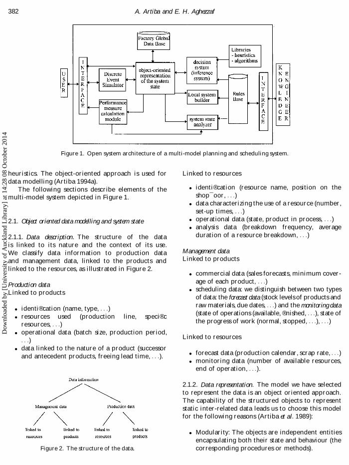
heuristics. The object-oriented approach is used fordata modelling (Artiba 1994a).

The following sections describe elements of themulti-model system depicted in Figure 1.

2.1. Object oriented data modelling and system state

2.1.1. Data description. The structure of the datais linked to its nature and the context of its use.We classify data information to production dataand management data, linked to the products andlinked to the resources, as illustrated in Figure 2.

Production dataLinked to products

E identi® cation (name, type, . . .)E resources used (production line, speci® c

resources, . . .)E operational data (batch size, production period,

. . .)E data linked to the nature of a product (successor

and antecedent products, freeing lead time, . . .).

Linked to resources

E identi® cation (resource name, position on theshop¯ oor, . . .)

E data characterizing the use of a resource (number,set-up times, . . .)

E operational data (state, product in process, . . .)E analysis data (breakdown frequency, average

duration of a resource breakdown, . . .)

Management dataLinked to products

E commercial data (sales forecasts, minimum cover-age of each product, . . .)

E scheduling data: we distinguish between two typesof data: the forecast data (stock levels of products andraw materials, due dates, . . .)and the monitoring data(state of operations (available, ® nished, . . .), state ofthe progress of work (normal, stopped, . . .), . . .)

Linked to resources

E forecast data (production calendar, scrap rate, . . .)E monitoring data (number of available resources,

end of operation, . . .).

2.1.2. Data representation. The model we have selectedto represent the data is an object oriented approach.The capability of the structured objects to representstatic inter-related data leads us to choose this modelfor the following reasons (Artiba et al. 1989):

E Modularity: The objects are independent entitiesencapsulating both their state and behaviour (thecorresponding procedures or methods).

A. Artiba and E. H. Aghezzaf382

Figure 1. Open system architecture of a multi-model planning and scheduling system.

Figure 2. The structure of the data.

Dow

nloa

ded

by [

Uni

vers

ity o

f A

uckl

and

Lib

rary

] at

14:

28 0

8 O

ctob

er 2

014

E Description close to reality: Natural representa-tion of the objects described (machines, products,. . .), resulting in better ergonomy, representationfacility, extendibility and performance.

E Possibility of giving default values: This allowsreasoning with incomplete data.

In production management, the data can be organ-ized in a set of hierarchical objects. Such a hierarchicalstructure then leads to a tree-structure in which theproperties can be transmitted from the root to theleaves (inheritance notion).

Alasuvanto et al. (1988) present two productionmanagement systems developed with an object-orientedprogramming and give the advantages of using suchprogramming language. Further details on object-oriented programming can be found in Cox (1986).

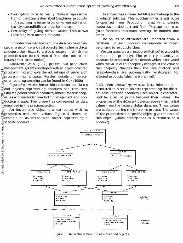
Figure 3 shows the hierarchical structure of classesand objects representing products and resources.Objects (resources and products) inherit speci® c prop-erties and methods from both management and pro-duction classes. The properties correspond to datadescribed in the previous section.

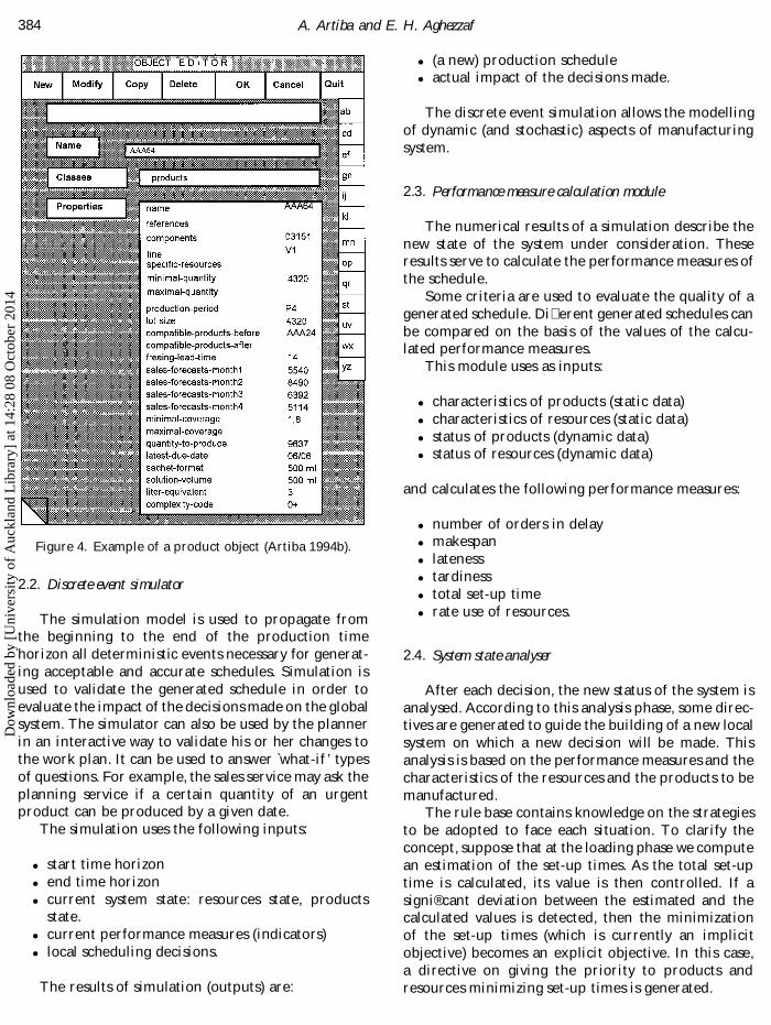
An instantiated object is a real object with itsproperties and their values. Figure 4 shows anexample of an instantiated object representing aspeci® c product.

This object has a name (AAA64)and belongs to theproducts’ subclass. This subclass inherits attributes(properties) from Production’ class (line, speci® cresources, lot- size, . . .) and from Management’ class(sales forecasts, minimum coverage in months, duedates, . . .).

The values of attributes are imported from adatabase. To each product corresponds an objectbelonging to products’ class.

We can associate a procedure (Method)to a speci® cattribute (or property). The property quantity- to-produce’ is associated with a demon which is activatedwhen the value of this property changes. If the value ofthis property changes then the level-of- stock andlatest-due-date are automatically recalculated fora� ected products (which are planned).

2.1.3. Object oriented system state. Data information istranslated to a set of objects representing the differ-ent resources and products. Each object is character-ized by a set of properties and their values. Theproperties of the di� erent objects receive their initialvalues from the factory global database. These valuesare updated during the inference process. The valuesof the properties of a speci® c object give the state ofthis object (which corresponds to a resource or aproduct).

An architecture of a multi-model system for planning and scheduling 383

Figure 3. Hierarchical structure of classes and objects.

Dow

nloa

ded

by [

Uni

vers

ity o

f A

uckl

and

Lib

rary

] at

14:

28 0

8 O

ctob

er 2

014

2.2. Discrete event simulator

The simulation model is used to propagate fromthe beginning to the end of the production timehorizon all deterministic events necessary for generat-ing acceptable and accurate schedules. Simulation isused to validate the generated schedule in order toevaluate the impact of the decisions made on the globalsystem. The simulator can also be used by the plannerin an interactive way to validate his or her changes tothe work plan. It can be used to answer what- if ’ typesof questions. For example, the sales service may ask theplanning service if a certain quantity of an urgentproduct can be produced by a given date.

The simulation uses the following inputs:

E start time horizonE end time horizonE current system state: resources state, products

state.E current performance measures (indicators)E local scheduling decisions.

The results of simulation (outputs) are:

E (a new) production scheduleE actual impact of the decisions made.

The discrete event simulation allows the modellingof dynamic (and stochastic) aspects of manufacturingsystem.

2.3. Performance measure calculation module

The numerical results of a simulation describe thenew state of the system under consideration. Theseresults serve to calculate the performance measures ofthe schedule.

Some criteria are used to evaluate the quality of agenerated schedule. Di� erent generated schedules canbe compared on the basis of the values of the calcu-lated performance measures.

This module uses as inputs:

E characteristics of products (static data)E characteristics of resources (static data)E status of products (dynamic data)E status of resources (dynamic data)

and calculates the following performance measures:

E number of orders in delayE makespanE latenessE tardinessE total set-up timeE rate use of resources.

2.4. System state analyser

After each decision, the new status of the system isanalysed. According to this analysis phase, some direc-tives are generated to guide the building of a new localsystem on which a new decision will be made. Thisanalysis is based on the performance measures and thecharacteristics of the resources and the products to bemanufactured.

The rule base contains knowledge on the strategiesto be adopted to face each situation. To clarify theconcept, suppose that at the loading phase we computean estimation of the set-up times. As the total set-uptime is calculated, its value is then controlled. If asigni® cant deviation between the estimated and thecalculated values is detected, then the minimizationof the set-up times (which is currently an implicitobjective) becomes an explicit objective. In this case,a directive on giving the priority to products andresources minimizing set-up times is generated.


Figure 4. Example of a product object (Artiba 1994b).

Dow

nloa

ded

by [

Uni

vers

ity o

f A

uckl

and

Lib

rary

] at

14:

28 0

8 O

ctob

er 2

014


E performance measuresE characteristics of resources and productsE analysis knowledge

and produces as output:

E directives to the local system builder.

2.5. Local system builder

The selection of products and resources to con-struct a local system depends on the global system state(performance indicators) and the objectives to meet.These objectives are expressed into the directivesgenerated by the system state analyser module.

Speci® c knowledge (expert’s rules) on the manu-facturing system under consideration, stored in therule base, is used in this product and resource selectionphase. These expert’s rules contain some preferencesor priorities given to some products and/or resources.For instance, in the pharmaceutical industry oneavoids for the last period (or shift) of a day planningthe production of a high cost solution, because if thereis a disturbance this solution will be lost. Anotherexample concerning allocation of resources is toschedule urgent products on the most reliableresources.


E characteristics of products and resourcesE directivesE expert’s rules

and provides the following results:

E selected productsE selected resources

which constitute a local search space.

2.6. Decision system

Depending on a local system con® guration, anoptimization algorithm or heuristic will be applied tosolve the given local problem. This analysis and selec-tion (of algorithms or heuristics) phase is achieved byusing expert rules. The expert rules are used to analysethis sub-problem (optimization criterion, constraintsand search space size) and activate the appropriatealgorithm or heuristic stored in the system libraries. If

a sub-problem doesn’t ® t the stored algorithms andheuristics, a general heuristic will be applied. Thisgeneral heuristic is based on constraint satisfactionto ® nd a feasible solution.

The second phase consists of activating the simula-tion module in order to validate the proposed solutionand to analyse the impact of this local solution on theglobal system. This step by step validation limitsrepetitive backtracking.


E a local sub-problemE characteristics of relevant products and resourcesE expert rulesE libraries of algorithms and heuristics

and produces results of scheduling decision:

E start and ® nish dates of each productE allocated resourcesE set-up timesE quantity of each product.

2.7. Libraries

The system libraries are external functions, eachone corresponding to a speci® c algorithm or heuristic.These executable functions can be activated by anyroutine. The interface protocol has to be respected(number, type and order of parameters).

A called function receives (as inputs) a list ofparameters describing the sub-problem to be solvedand returns (as outputs), a list of parameters describingthe solution of the problem, i.e. a scheduling decision.

2.8. Rule base

This knowledge base is divided into three areas.Each area or set of expert rules is dedicated to aspeci® c functional module using it. These areas are:

(1) A set of rules used by the Decision System: Theserules describe the conditions of the selection ofthe appropriate algorithm or heuristic used tosolve the sub-problem.

(2) A set of rules used by the Local System Builder:Expert rules speci® c to the manufacturingsystem under consideration. They are used inthe selection of products and resources.

(3) A set of rules used by the System State Analyzer:Analysis knowledge which serves to generatesome directives concerning the status of thesystem.


ownl

oade

d by

[U

nive

rsity

of

Auc

klan

d L

ibra

ry]

at 1

4:28

08

Oct

ober

201

4

2.9. Interfaces

The expert or knowledge engineer uses speci® cinterfaces to create or update the knowledge base(rules and objects). The planner uses speci® c inter-faces to access the workplan, to simulate the impact ofsome modi® cations or to display some performancemeasures.

The man-machine communication interfaces arevery important and are decisive for acceptance of thesystem by the end user. A special attention has beenpaid to this aspect as explained in Bourgeois et al.(1993).

Another important feature is the integration of thesystem in the existing environment of the factory.

2.10. Factory global data base

This Factory Global Data Base is a set of ® les anddata bases representing the factory informationsystem.

3. The operational architecture of the system

The implementation of a speci® c application withthe multi-model system requires an understanding ofits development language. We describe the functional-ities and the syntax of this language.

3.1. Internal language

The system language has a Pascal- like syntax forreadability and maintainability reasons. This languagepermits the use of (not an exhaustive list):

E arithmetical expressions (operators: + , - , /, *,SQRT, . . .)

E Boolean expressions (operators: and, or, not, > , < ,. . .)

E universal and existential operators (for any . . .)E union and intersection (applied to lists or sets of

objects)E external procedures and functions callE description of classes and objectsE loops (while condition do action)E if condition then action rules (extended produc-

tion rules where time is considered)E read (and write)data from (into) external ® lesE functions like: min, max, ® rst and last (element of

list), . . .E string of characters.

This internal language is a functional language.This means that after checking the internal syntax,the code will be replaced by the di� erent existingfunctions stored in the speci® c libraries.

3.2. Implementation of speci® c application

After the analysis and modelling phases of theplanning and scheduling problem under considera-tion, the user can implement his or her speci® capplication with the language described above.

The user should describe:

E resources of the manufacturing system underconsideration and their characteristics (classesand objects with their properties)

E products to manufacture (properties, routeing)E constraintsE objective(s) (classi® cation if more than one)E speci® c knowledgeE horizonE interface ultimately with other applicationsE interface with factory information system.

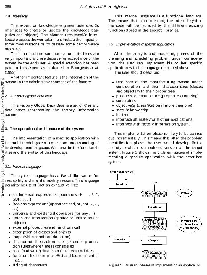
This implementation phase is likely to be carriedout incrementally. This means that after the problemidenti® cation phase, the user would develop ® rst aprototype which is a reduced version of the targetsystem. Figure 5 shows the di� erent stages of imple-menting a speci® c application with the describedsystem.


Figure 5. Di� erent phases of implementing an application.

Dow

nloa

ded

by [

Uni

vers

ity o

f A

uckl

and

Lib

rary

] at

14:

28 0

8 O

ctob

er 2

014

Once the application has been described with theinternal language, the syntax is veri® ed and the inter-nal code is translated to the programming language (inour case, C+ + ). The source code in programminglanguage is then compiled and the external functionsare incorporated to produce an executable ® le.

This way of implementation is very interesting forthe following reasons:

E the system is hardware independentE the architecture is open, and it easily permits

extension of the functionalities of the systemE the executable code is fast.

In the following section a hybrid shop schedulingproblem, solved using a limited version of the pro-posed multi-model approach, is presented.

4. Application: hybrid ¯owshop planning andscheduling problem

The industrial case chosen for this application ofthe multi-model approach is a chemical plant whichproduces herbicides. The production of herbicides inthis facility is done in two stages: formulation andconditioning (® lling and packaging). This is a typicalhybrid ¯ owshop problem. A hybrid ¯ owshop consistsof a series of production stages, each of which hasseveral facilities operating in parallel. This structure isvery common in production and packaging of liquid orpowder products so this case can be extended to otherindustrial cases with minor modi® cations.

4.1. The formulation units

Formulation consists of composing a chemicalsolution with precise amounts of constituents.

In the formulation units herbicides are formulatedand mixed in tanks. For each tank a minimum size ofthe batch to be mixed is required (this is due to mixingand contamination constraints)and there is of course amaximum batch size which is the capacity of the tank.

Mixing a batch takes approximately the same timeregardless of its size, moreover cleaning and analysingtimes are constant. After the formulation herbicidescan be sent to ® lling lines or transferred into holdtanks. Each tank is dedicated to one family of herbi-cides. The tanks are linked together and connected tothe ® lling lines.

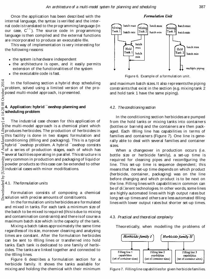
Figure 6 describes a formulation section for aherbicide family. It shows the tanks available formixing and holding the chemical with their minimum

and maximum batch sizes. It also represents the pipingconstraints that exist in the section (e.g. mixing tank 2and hold tank 1 have the same piping).

4.2. The conditioning section

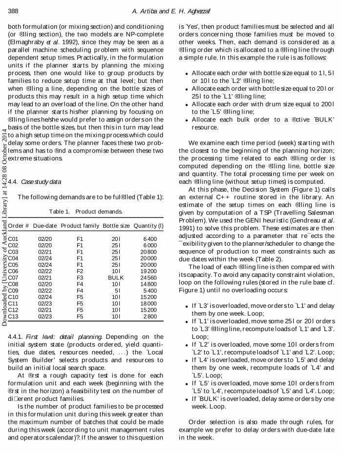
In the conditioning section herbicides are pumpedfrom the hold tanks or mixing tanks into containers(bottles or barrels) and the containers are then pack-aged. Each ® lling line has capabilities in terms offamilies and containers (Figure 7). One line is gene-rally able to deal with several families and containersizes.

When a changeover in production occurs (i.e.bottle size or herbicide family), a set-up time isrequired for cleaning pipes and recon® guring theline. This set-up time is sequence dependent; thismeans that the set-up time depends on which product(herbicide, container, packaging) was on the linebefore changing and which product is to be next onthe line. Filling lines with capabilities in common canbe of di� erent technologies. In other words, some linesare highly automated lines with high output rates butlong set-up times and others are less automated ® llinglines with lower output rates but shorter set-up times.

4.3. Practical and theoretical complexity

Theoretically, when modelling the problems of


Figure 6. Example of a formulation unit.

Figure 7. Filling line capabilities for given herbicide families.

Dow

nloa

ded

by [

Uni

vers

ity o

f A

uckl

and

Lib

rary

] at

14:

28 0

8 O

ctob

er 2

014

both formulation (or mixing section)and conditioning(or ® lling section), the two models are NP-complete(Elmaghraby et al. 1992), since they may be seen as aparallel machine scheduling problem with sequencedependent setup times. Practically, in the formulationunits if the planner starts by planning the mixingprocess, then one would like to group products byfamilies to reduce setup time at that level; but thenwhen ® lling a line, depending on the bottle sizes ofproducts this may result in a high setup time whichmay lead to an overload of the line. On the other handif the planner starts his/her planning by focusing on® lling lines he/she would prefer to assign orders on thebasis of the bottle sizes, but then this in turn may leadto a high setup time on the mixing process which coulddelay some orders. The planner faces these two prob-lems and has to ® nd a compromise between these twoextreme situations.

4.4. Case study data

The following demands are to be ful® lled (Table 1):

4.4.1. First level: detail planning. Depending on theinitial system state (products ordered, yield quanti-ties, due dates, resources needed, . . .) the LocalSystem Builder’ selects products and resources tobuild an initial local search space.

At ® rst a rough capacity test is done for eachformulation unit and each week (beginning with the® rst in the horizon) a feasibility test on the number ofdi� erent product families.

Is the number of product families to be processedin this formulation unit during this week greater thanthe maximum number of batches that could be madeduring this week (according to unit management rulesand operators calendar)?. If the answer to this question

is Y es’, then product families must be selected and allorders concerning those families must be moved toother weeks. Then, each demand is considered as a® lling order which is allocated to a ® lling line througha simple rule. In this example the rule is as follows:

E Allocate each order with bottle size equal to 1 l, 5 lor 10 l to the L2’ ® lling line;

E Allocate each order with bottle size equal to 20 l or25 l to the L1’ ® lling line;

E Allocate each order with drum size equal to 200 lto the L5’ ® lling line;

E Allocate each bulk order to a ® ctive BULK’resource.

We examine each time period (week) starting withthe closest to the beginning of the planning horizon;the processing time related to each ® lling order iscomputed depending on the ® lling line, bottle sizeand quantity. The total processing time per week oneach ® lling line (without setup times) is computed.

At this phase, the Decision System (Figure 1) callsan external C+ + routine stored in the library. Anestimate of the setup times on each ® lling line isgiven by computation of a TSP (Travelling SalesmanProblem). We used the GENI heuristic (Gendreau et al.1991) to solve this problem. These estimates are thenadjusted according to a parameter that re¯ ects the¯ exibility given to the planner/scheduler to change thesequence of production to meet constraints such asdue dates within the week (Table 2).

The load of each ® lling line is then compared withits capacity. To avoid any capacity constraint violation,loop on the following rules (stored in the rule base cf.Figure 1) until no overloading occurs:

E If L3’ is overloaded, move orders to L1’ and delaythem by one week. Loop;

E If L1’ is overloaded, move some 25 l or 20 l ordersto L3’ ® lling line, recompute loads of L1’ and L3’.Loop;

E If L2’ is overloaded, move some 10 l orders fromL2’ to L1’, recompute loads of L1’ and L2’. Loop;

E If L4’ is overloaded, move orders to L5’ and delaythem by one week, recompute loads of L4’ andL5’. Loop;

E If L5’ is overloaded, move some 10 l orders fromL5’ to L4’, recompute loads of L5’ and L4’. Loop;

E If BULK’ is overloaded, delay some orders by oneweek. Loop.

Order selection is also made through rules, forexample we prefer to delay orders with due-date latein the week.


Table 1. Product demands.

Order # Due-date Product family Bottle size Quantity (l)

C01 02/20 F1 20 l 6 400C02 02/20 F1 25 l 6 000C03 02/21 F1 25 l 20 800C04 02/24 F1 25 l 20 000C05 02/24 F1 25 l 20 000C06 02/22 F2 10 l 19 200C07 02/21 F3 BULK 24 560C08 02/20 F4 10 l 14 800C09 02/22 F4 5 l 5 400C10 02/24 F5 10 l 15 200C11 02/23 F5 10 l 18 000C12 02/21 F5 10 l 15 200C13 02/23 F5 10 l 2 800

Dow

nloa

ded

by [

Uni

vers

ity o

f A

uckl

and

Lib

rary

] at

14:

28 0

8 O

ctob

er 2

014


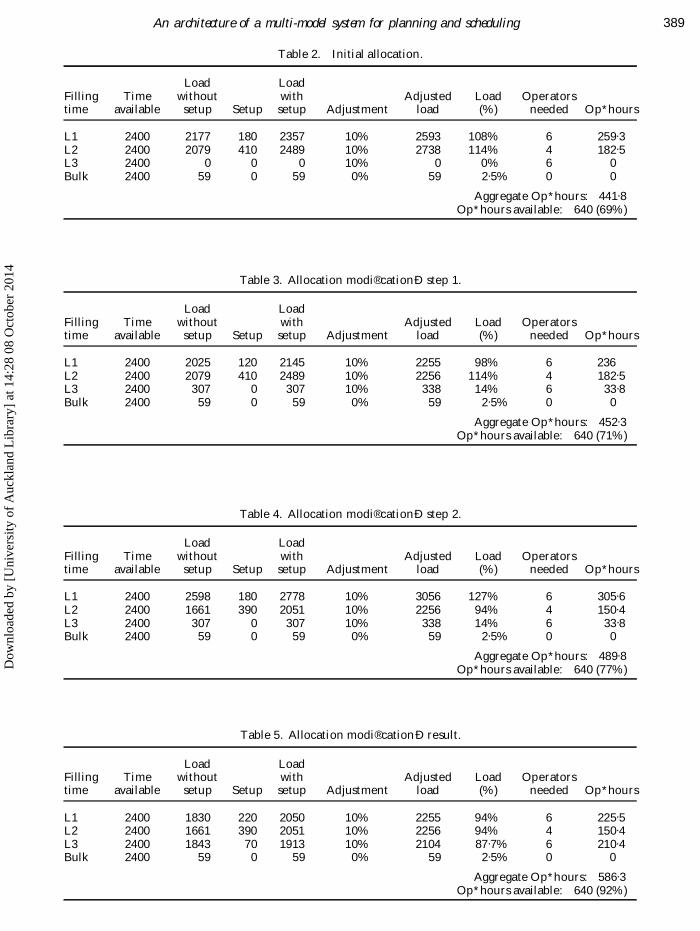
Table 2. Initial allocation.

Load LoadFilling Time without with Adjusted Load Operatorstime available setup Setup setup Adjustment load (%) needed Op*hours

L1 2400 2177 180 2357 10% 2593 108% 6 259.3L2 2400 2079 410 2489 10% 2738 114% 4 182.5L3 2400 0 0 0 10% 0 0% 6 0Bulk 2400 59 0 59 0% 59 2.5% 0 0

Aggregate Op*hours: 441.8Op*hours available: 640 (69%)

Table 3. Allocation modi® cationÐ step 1.


L1 2400 2025 120 2145 10% 2255 98% 6 236L2 2400 2079 410 2489 10% 2256 114% 4 182.5L3 2400 307 0 307 10% 338 14% 6 33.8Bulk 2400 59 0 59 0% 59 2.5% 0 0


Table 4. Allocation modi® cationÐ step 2.


L1 2400 2598 180 2778 10% 3056 127% 6 305.6L2 2400 1661 390 2051 10% 2256 94% 4 150.4L3 2400 307 0 307 10% 338 14% 6 33.8Bulk 2400 59 0 59 0% 59 2.5% 0 0


Table 5. Allocation modi® cation Ð result.


L1 2400 1830 220 2050 10% 2255 94% 6 225.5L2 2400 1661 390 2051 10% 2256 94% 4 150.4L3 2400 1843 70 1913 10% 2104 87.7% 6 210.4Bulk 2400 59 0 59 0% 59 2.5% 0 0


Dow

nloa

ded

by [

Uni

vers

ity o

f A

uckl

and

Lib

rary

] at

14:

28 0

8 O

ctob

er 2

014

These rules are applied if a balancing problem isdetected (if one or more lines are overloaded).

For week 8 (20 ± 24 February), the di� erent steps arepresented in Tables 3 ± 5.

In the ® rst step order C01’ is moved from L1’ toL3’, consequently the aggregate load of L1’ decreasesto an acceptable level. However L2’ remains over-loaded (Table 3).

In the second step order C08’ is removed from L2’and allocated to L1’; this implies a decrease in the loadof L2’ which is therefore not overloaded any more butthe extra load on L1’ leads to an overload of this ® llingline (Table 4).

In the last step C03’ and C04’ are moved from L1’to L3’. The aggregate load of every ® lling line is nowacceptable (Table 5).

When line capacity problems have been dealt with,operators aggregate availability is checked. For each® lling line the number of operators required to run itis given. So the number of operator hours can becomputed and compared to the total number ofoperator hours available. If the number of operatorhours exceeds the total available for the week, someorders should be brought forward if possible. If this isnot enough, overtime or extra operators might beallocated to some ® lling lines or at least some ordersshould be delayed.

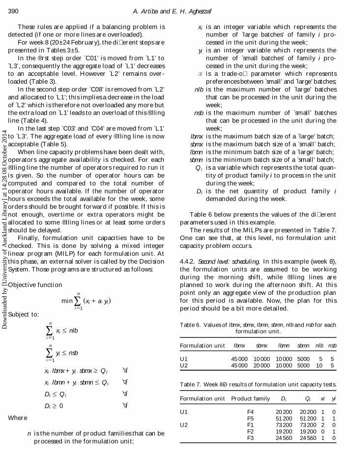
Finally, formulation unit capacities have to bechecked. This is done by solving a mixed integerlinear program (MILP) for each formulation unit. Atthis phase, an external solver is called by the DecisionSystem. Those programs are structured as follows:

Objective function

min Sn

i =1

(xi + a . yi)

Subject to:

Sn

i =1

xi £ nlb

Sn

i =1

yi £ nsb

xi . lbmx + yi . sbmx ³ Q i " i

xi . lbmn + yi . sbmn £ Q i " i

Di £ Q i " i

Di ³ 0 " i

Where

n is the number of product families that can beprocessed in the formulation unit;

xi is an integer variable which represents thenumber of large batches’ of family i pro-cessed in the unit during the week;

yi is an integer variable which represents thenumber of small batches’ of family i pro-cessed in the unit during the week;

a is a trade-o� parameter which representspreferences between small’ and large’ batches;

nlb is the maximum number of large’ batchesthat can be processed in the unit during theweek;

nsb is the maximum number of small’ batchesthat can be processed in the unit during theweek;

lbmx is the maximum batch size of a large’ batch;sbmx is the maximum batch size of a small’ batch;lbmn is the minimum batch size of a large’ batch;sbmn is the minimum batch size of a small’ batch;

Q i is a variable which represents the total quan-tity of product family i to process in the unitduring the week;

Di is the net quantity of product family idemanded during the week.

Table 6 below presents the values of the di� erentparameters used in this example.

The results of the MILPs are presented in Table 7.One can see that, at this level, no formulation unitcapacity problem occurs.

4.4.2. Second level: scheduling. In this example (week 8),the formulation units are assumed to be workingduring the morning shift, while ® lling lines areplanned to work during the afternoon shift. At thispoint only an aggregate view of the production planfor this period is available. Now, the plan for thisperiod should be a bit more detailed.


Table 7. Week 8Ð results of formulation unit capacity tests.

Formulation unit Product family D i Qi xi yi

U1 F4 20 200 20 200 1 0F5 51 200 51 200 1 1

U2 F1 73 200 73 200 2 0F2 19 200 19 200 0 1F3 24 560 24 560 1 0

Table 6. Values of lbmx, sbmx, lbmn, sbmn, nlb and nsb for eachformulation unit.

Formulation unit lbmx sbmx lbmn sbmn nlb nsb

U1 45 000 10 000 10 000 5000 5 5U2 45 000 20 000 10 000 5000 10 5

Dow

nloa

ded

by [

Uni

vers

ity o

f A

uckl

and

Lib

rary

] at

14:

28 0

8 O

ctob

er 2

014

First of all, orders will be associated with batches.The number and product family of the batches toformulate in each unit are known from the formula-tion unit capacity test. The allocation rule is presentedbelow (for each unit):

E If there are orders concerning the U1 unit allocatethose orders by priority of due-date to the ® rstbatch of the same product family not yet full.

E If there are orders concerning the U2 unit allocatethose orders by priority of due-date to the ® rstbatch of the same product family not yet full.

Note that orders might have to be split betweenseveral batches due to the minimum or maximumbatch size constraints i.e. C04 and C12 in this case(Table 8).

The batch number is the sequence order. In unit`U2’ there are two large mixing tanks. Large batch #1-1and Large batch #2-1 are formulated in distinct mixingtanks. These formulations might therefore be carriedout simultaneously. At this point, a management rule isadopted which consists of transferring into hold tanksevery formulated batch as a whole whenever it ispossible. The resolution of a TSP on each ® lling linegives a sequence of orders or rather a sequence ofgroups of orders. For example the sequence of orderson L3’ obtained by solving the TSP problem with theGENI’ heuristic is C01 ® C03 ® C04, but in fact werepresent this sequence as follows:

C01 C03;C04

This means that in terms of setup cost,C01 ® C03 ® C04 is equal to C01 ® C04 ® C03. It isalso equal to C03 ® C04 ® C01 or C04 ® C03 ® C01.The orders to be placed on the L2’ are in fact:

C09 C10; C11; C12-1;C12-2; C13

The sequence on this line is constructed by pickingfrom the set of orders which can be placed on the line(according to the constraints coming from the groupsequences), the order with the nearest due-date

(applying EED-Earliest Due Date heuristic). Thesequences on the di� erent lines obtained in thisexample are presented in Table 9.

Those results feed a simulation model that includesan accurate description of the production system,constraints and elementary management rules, mostof which could not be easily taken into account beforethis stage. The simulation results in positioning theorders on the horizon. Performance measures arecollected in order to qualify the solution found andthus proposals for improvement are generated.

In this example we took into account two groups ofperformance measures: Cmax (maximum completiontime)and total idle time for each resource. Accordingto the values of these criteria a local system is builtaccording to the analysis done by the System StateAnalyser which runs at this stage with some simplerules such as:

E Select the ® lling line with Maximum Cmax and themixing tank associated with it for the order thatfollows the longest idle time. Let’s name this orderOf.

Proposals for improvement are made. These proposalsare such as:

E Delay one order associated with the same holdtank than the one from which order (Of ) isproduced and whose conditioning has startedbefore the idle time begins. Create a new batchassociated with (Of ) to be formulated later.

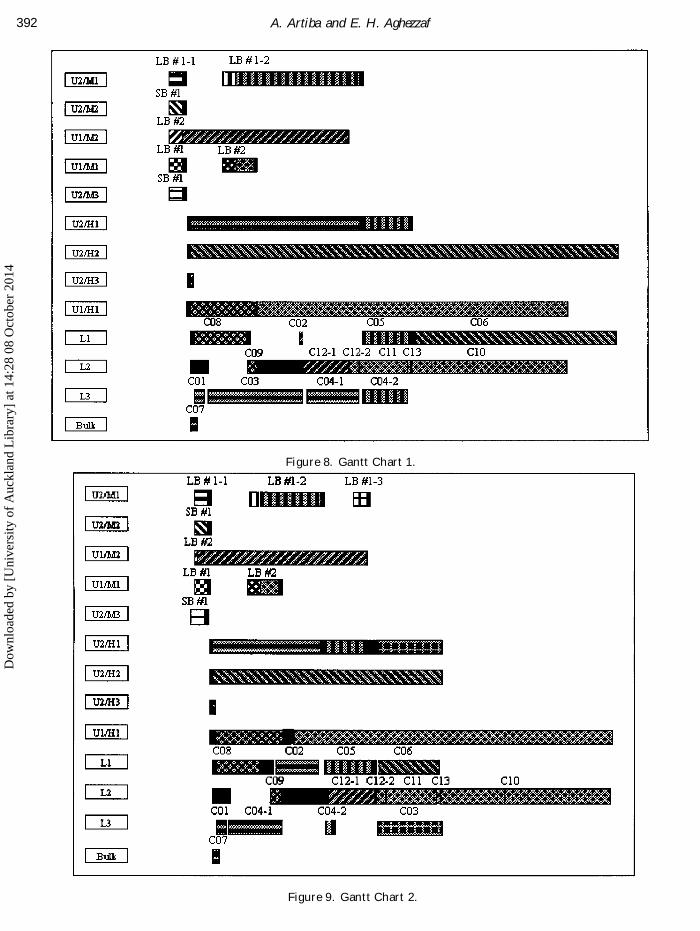
The solution of simulation is represented as a Ganttchart (Figure 8).


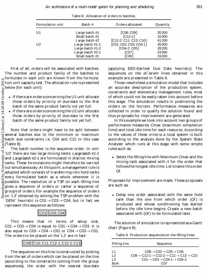
Table 8. Allocation of orders to batches.

Formulation unit Batch # Orders allocated Quantity

U1 Large batch #1 {C08; C09} 20 200Small batch #1 {C12-1} 10 000Large batch #2 {C12-2; C11; C13; C10} 41 200

U2 Large batch #1-1 {C01; C02; C03; C04-1} 45 000Large batch #1-2 {C04-2; C05} 28 200Large batch #2-1 {C07} 24 560Small batch #1 {C06} 19 200

Table 9. Production sequences on the ® lling lines.

Filling line Sequence

L1 C08 ® C02 ® C05 ® C06L2 C09 ® C12-1 ® C12-2 ® C11 ® C13 ® C10L3 C01 ® C03 ® C04-1 ® C04-2Bulk C07

Dow

nloa

ded

by [

Uni

vers

ity o

f A

uckl

and

Lib

rary

] at

14:

28 0

8 O

ctob

er 2

014


Figure 8. Gantt Chart 1.

Figure 9. Gantt Chart 2.

Dow

nloa

ded

by [

Uni

vers

ity o

f A

uckl

and

Lib

rary

] at

14:

28 0

8 O

ctob

er 2

014

Here the local system is composed of L1’ and `Holdtank 1’. The order C03’ is moved and a new batch isinserted in `Mixing tank 1’ (Figure 9).

The result of this action is stored as it leads to animprovement of the situation. This loop is repeateduntil the ® nal result is satisfying or a ® xed number ofiterations is reached. The tools used to solve this caseare C+ + , SLAM II and Microsoft Excell. It takes about5 minutes to get a solution on a PC 486/66.

5. Conclusion

In this paper we have presented the architecture ofa multi-model system for production planning andscheduling. This approach is applied for planningand scheduling in a chemical plant, which presentssome interesting properties. We show how detailed aplan may be achieved using some of the multi-modelfunctionalities (simulation, rules . . .). Once the aggre-gate plan is produced, the scheduling level is thentackled. Here again some of the multi-model function-alities are employed using di� erent models (MILP,heuristics, rules, . . .).

The multi-model approach is very promising forthe solution of industrial problems. We continue totackle di� erent industrial problems with this multi-model approach in order to improve our know-how inthis ® eld and ® nd the appropriate methods for thespeci® c problems.

Acknowledgements

This research project is supported by funds fromWallonie region (MinisteÁ re du DeÂ veloppement Tech-nologique et de l’Emploi). We would like to thankOlivier Kaufmann and Philippe Levecq for their col-laboration in the chemical plant application.

References

ALASUVANTO, J., ELORANTO, E., FUY UKI, M., KIDA, T., andINOUE, I., 1988, Object oriented programming in produc-tion management-two pilot systems. International Journal ofProduction Research, 26, 765± 776.

ARTIBA, A., TAHON, C., SOENEN, R., and VANDEPEUTTE, G.,1989, BAXPES: An Expert System for planning

Manufacturing lines. In Proceedings of the Society of ComputerSimulation International, San Diego, California, pp. 79± 83.

ARTIBA, A., and TAHON, C., 1992, Production planningknowledge-based system for pharmaceutical manufactur-ing line. European Journal of Operational Research, 61, 18± 29.

ARTIBA, A., 1994A, Towards a multi-model approach forproduction planning and control systems. EURO XIIIConference, July 1994, Glasgow, UK.

ARTIBA, A., 1994B, A rule-based planning system for parallelmultiproduct manufacturing lines. Production Planning andControl, 5, 349± 359.

BOOCH, G., 1991, Object Oriented Design with Applications(Benjamin Cummings Publishing Co., Redwood City, CA).

BOURGEOIS, S., ARTIBA, A., and TAHON, C., 1993, Decisionsupport system for dynamic job-shop scheduling. Revue dessysteÁ mes de deÂ cision, 2, 277± 292.

COAD, P., and Y OURDON, E., 1992, Analyse Orientee Objets(Masson Prentice Hall, Paris).

COX, B. J., 1986, Object Oriented ProgrammingÐ An EvolutionaryApproach (Addison± Wesley, Reading, MA).

DULGERI, Z., D’ALESSANDRO, G., and MAGALETTI, N., 1993, Ahierarchical knowledge-based scheduling and control forFMSs. International Journal of Computer Integrated Manufactur-ing, 6, 191± 200.

ELMAGHRABY , S. E., GUINET, A., and SCHELLENBERGER, K. W.,1992, Sequencing on Parallel Processors: An AltemateApproach. O.R. technical report, (1992)#273, OperationalResearch and Industrial Engineering, North Carolina StateUniversity, Raleigh, USA.

FALSTER, P., 1987, Planning and controlling productionsystems combining simulation and expert systems. Com-puters in Industry, 8, 161± 172.

GENDREAU, M., HERTZ, A., and LAPORTE, G., 1991, NewInsertion and Post-Optimization, Procedures for the tra-velling salesman, Problem. Centre de recherche sur lestransports, UniversiteÂ de MontreÂ al, QueÂ bec.

KUSIAK, A., 1987, Designing expert systems for scheduling ofautomated manufacturing. Industrial Engineering, 19, 42± 46.

MEYER, B., 1990, Conception et programmation par Objet (Inter-Editions, Paris).

MULLER, H., DE SAMBLANCKX, S., and MATTHY S, D., 1987, Theexpert system approach and the ¯ exibility-complexityproblem in scheduling production systems. InternationalJournal of Production Research, 25, 1659± 1670.

KADABA, N., KENDALL, E., and JUELL, P. L., 1991, Integration ofadaptive machine learning and knowledge-based systemsfor routing and scheduling applications. Expert Systems WithApplications, 2, 15± 27.

O’KEEFE, R. M., 1985, Expert Systems and OperationalResearchÐ Mutual Bene® ts. Journal of the OperationalResearch Society, 36, 125± 129.

RUMBAUGH, J., BLAHA, M., PREMERLANI, W., EDDY , F., andLORENSEN, W., 1991, Object-Oriented Modelling and Design(Prentice Hall, Englewood Cli� s, NJ).

SMITH, S. F., 1992, Knowledge-based production manage-ment: approaches, results and prospects. Production Plan-ning and Control, 3, 350± 380.


ownl

oade

d by

[U

nive

rsity

of

Auc

klan

d L

ibra

ry]

at 1

4:28

08

Oct

ober

201

4

an architecture of a multi-model system for planning and scheduling

Documents