an approach towards parallelisation of sequential programs in an interactive environment

ELSEVIER Information and Software Technology 39 (1997) 77-89

lNHlRMA77DN AND

SOFTWARE TECHNOUHY

An approach towards parallelisation of sequential programs in an interactive environment

N. Mukherjee, P.K. Das

Department of Computer Science and Engineering, Jadavpur University, Calcultta - 700 032, India

Received 17 February 199.5; revised 8 February 1996; accepted 28 May 1996

Abstract

This paper presents an approach for extraction of functional parallelism from sequential programs in an interactive environment. It uses Hierarchical Task Graph (HTG) as an intermediate representation of a parallel program. This graph is constructed starting from the entire sequential program as its root node, considering both loop nodes and conditional nodes as its intermediate nodes and the basic blocks as the leaf nodes. During an interactive session, the user can move across different levels of the HTG and may test whether different nodes can be executed in parallel. The user can even cross the basic block boundary to increase the scope of parallelisation. Once the Control Flow Graph for parallel code generation is decided through such interaction, the Execution Conditions for the nodes of this graph are derived using an efficient method.

Keywords: Functional parallelism; Hierarchical task graph; Loop nodes; Conditional nodes; Interactive environment; Dependency analysis; Deriva-

tion of execution conditions

1. Introduction

With the proliferation of parallel computer architecture, exploiting parallelism for concurrent execution has become an important technique for improving computer system performance. However, this also demands greater involvement on the part of programmers as parallelism can be exploited only with substantial programming effort. During the last few years, significant research work [l-4] has been carried out with a view to improving compiler technology, so that programmers can obtain the benefits of enhanced performance from application programs written in sequential high level languages. It can then be left to the compiler and the operating system at run time to worry about different aspects of the architecture and the intricacies of parallel execution and to extract parallelism from sequential programs.

Two different approaches exist for extracting parallelism from sequential programs. One is to concentrate on the parallelism inherent in loops. This type of parallelism results from carrying out repetitive operations on a large number of data values. On this a great deal of research work has been carried out [4,5-71. The other approach is the extraction of non-loop parallelism or functional

0950-5849/97/$15.00 0 1997 Elsevier Science R.V. All rights reserved PII SO950-5849(96)01129-9

parallelism. It is program-driven rather than data-driven as in the former approach [2,3,8]. Comparatively less work has been done on this approach. Functional

parallelism is extracted by effectively decomposing the sequential program into a numer of parallel tasks. These tasks are to run on different processors so that both the program segments as well as the data sets on which these processors work are different, although there remain strict precedence constraints. Hence this approach is inherently more suitable for execution on loosely coupled, distributed memory multiple instruction multiple data (MIMD) systems. Significant contribution to extract functional parallelism was made in [9,3].

In most of these previous works, however, attempts have been made to carry out extraction of parallelism, code generation and scheduling automatically [2,9]. The major drawback of such automatic detection of parallelism is the automatic adjustment of the task granularity and conservative dependence analysis. In automatic tools, granularity is either predefined or is adjusted automatically. There is little scope to work with different granularities. Again, during the dependency analysis phase, if it cannot be proven that a dependence does not exist, automatic tools tend to be conservative and assume a dependence. In all these situations, the

18 N. Mukherjee, P.K. Dasllnformation and Software Technology 39 (1997) 77-89

programmer, having adequate knowledge about the overall semantics of the program, is often able to solve the problem of the specific dependence more efficiently. The programmer’s interaction would therefore help the system to generate more efficient parallel programs than the automatic tools working alone.

2. The Hierarchical Task Graph

This paper presents a methodology to parallelise application programs for a distributed memory MIMD system under an interactive environment. Extraction of parallelism is done with the help of a Hierarchical Task Graph (HTG) that specifies parallelism at various levels of granularity. HTG is formally defined and discussed in the next section. Unlike [IO], however, our HTG is not based on loops alone, but also considers conditional nodes. Thus, while constructing the HTG, loop nodes as well as conditional nodes contribute to generating the intermediate nodes of the HTG. In the next section we discuss different aspects of the HTG and the construction of the HTG based on loops and conditional nodes.

For several years after the introduction of MIMD computers, the task graph, a directed acyclic graph, has continued to be used as a model for parallel programs. The task graph remains very useful for the analysis, scheduling and simulation of parallel programs. It is a powerful model for the extraction of loop level parallelism. But whenever we shift our attention to the non-loop parallelism, we feel the need for a more efficient and powerful representation of the programs. The HTG, which basically consists of task graph representations of different nodes at various hierarchical levels, comes out as a powerful representation of programs for the extraction of functional parallelism.

After completing the construction of the HTG, an interactive environment is created by the system and the user can test different parallelising strategies to find out some optimal parallel code for the program. The user can move to different levels of the HTG, thus changing the task granularity, and can explore the scope of parallelisation of various nodes of the HTG. To maxi- mize the scope of parallelisation, the user may even choose to cross the basic block boundary and split the basic block into two (and subsequently more) different nodes. Thus in an interactive environment the task gran-

ularity is determined by the user’s suggestion and intervention. To assist the user in deciding the task granularity, some estimates about the execution time of each node are also provided to the user by the system. Our approach exploits the domain knowledge of the programmer regarding the application area. The user, having the overall knowledge about the operational aspects of the program, can complement the pro- grammed intelligence of the paralleliser significantly and can help the system analyse the dependency more effectively by supplying the information such as loop bounds, array subscripts etc. which are not available at compile time. In some cases, the user can also increase the scope of parallelisation by removing dependencies through such interactions wherever possible. These and various other aspects of the interactive environment are discussed in Section 3.

Any sequential program can be partitioned into strongly connected regions based on loops in such a way that a hierarchical structure can be defined on it [9]. Each node in this hierarchical structure is identified as a task that consists of subtasks. The root node of the HTG corresponds to the entire sequential program. Par- titioning the root node, we get a set of intermediate nodes which are contained in the next level of the HTG. In [9], intermediate nodes are described, constructed from strongly connected regions based on loops. In this paper, we introduce the concept of conditional nodes which also contribute to form the intermediate nodes of the HTG. Loop nodes and conditional nodes are formally defined later in this section. Each of these intermediate nodes can again be partitioned to obtain the nodes in the next level. We continue in this fashion until we reach the basic blocks [ll]. Basic blocks form the leaf nodes of the HTG. Thus a layered graph can be built up with a recursive structure, where each layer consists of control flow graphs similar to those in the original sequential programs. The only difference is that the control flow graphs of HTG nodes at different levels of the HTG are acyclic.

In the interactive environment, the user decides the initial Control Flow Graph (CFG). This CFG is then analysed to obtain the execution condition of each node. Details of the derivation of execution conditions of nodes are discussed in Section 4.

The HTG is a powerful intermediate representation of a program. The importance of the HTG in the detection and management of parallelism was first recognised in [ 121. The construction of intermediate nodes from strongly connected regions was suggested in [13] and later developed in [14]. This approach was followed in [9] for building the task graph. The hierarchical structure was constructed on the basis of loops. Reducible programs [l l] can easily be mapped into a hierarchical structure based on loops where loops have well defined iteration bodies with a single entry and a single exit point. It has been shown in [9] that programs can be transformed in such a way that all types of loops change to single entry-single exit loops.

In Section 5, we consider some actual programs and In our approach the loops in a sequential program are

apply the methodologies prescribed in this paper to identified first, followed by strongly connected regions extract parallelism from them. Concluding remarks and based on these loops. Next, we identify the conditional

scope for future work are presented in Section 6. nodes. From this set of loop nodes and conditional

N. Mukherjee, P.K. Dasllnformation and Software Technology 39 f 1997) 77-89 79

nodes, the HTG is constructed. As stated above, this HTG is a directed acyclic graph whose root node corresponds to the control flow graph of the program from where we have started; leaf nodes correspond to the basic blocks of the program and all the intermediate nodes correspond to the strongly connected regions and conditional nodes. We can have the following types of nodes in the HTG.

1. Start node: has no incoming arcs, and there is a path from it to every node in the graph.

2. Stop node: has no outgoing arcs, and there is a path from every node in the graph to it.

3. Simple node: represents a task that has no subtasks. 4. Compound node: represents a task that consists of

other tasks in an HTG. 5. Loop node: represents a task that is a loop whose

iteration body is an HTG similar to the body of the compound node.

6. Conditional node: contains two or more different paths where each of these paths consists of other tasks.

The approach described in [9] is based on loops alone. There are sequential programs, however, where loops are either not used at all or only very few loops are used. For such programs, this approach unnecessarily limits the scope of parallelisation.

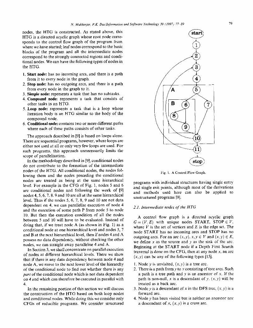
In the methodology described in [9], conditional nodes do not contribute to the formation of the intermediate nodes of the HTG. All conditional nodes, the nodes following them and the nodes preceding the conditional nodes are treated as being at the same hierarchical level. For example in the CFG of Fig. 1, nodes 5 and 6 are conditional nodes and following the work of [9] nodes 4,5,6,7,8,9 and 10 are all at the same hierarchical level. Thus if the nodes 5, 6, 7, 8, 9 and 10 are not data dependent on 4, we can parallelise execution of node 4 and the execution of some path P from node 5 to node 10. But then the execution condition of all the nodes between 5 and 10 will have to be evaluated. Instead of doing that, if we treat node A (as shown in Fig. 1) as a conditional node at one hierarchical level and nodes 5, 7 and B at the next hierarchical level, then if nodes 4 and A possess no data dependency, without checking the other nodes, we can straight away parallelise 4 and A.

In Section 3, we shall concentrate on parallel execution of nodes at different hierarchical levels. There we show that if there is any data dependency between node 4 and node A, we move to the next lower level of the hierarchy of the conditional node to find out whether there is any part of the conditional node which is not data dependent on 4 and which can therefore be executed in parallel with 4.

In the remaining portion of this section we will discuss the construction of the HTG based on both loop nodes and conditional nodes. While doing this we consider only CFGs of reducible programs. We consider structured

Fig. 1. A Control Flow Graph.

programs with individual structures having single entry and single exit points, although most of the derivations and methods used here can also be applied to unstructured programs [9],

2.1. Intermediate nodes of the HTG

A control flow graph is a directed acyclic graph G = (V, E) with unique nodes START, STOP E V, where V is the set of vertices and E is the edge set. The node START has no incoming arcs and STOP has no outgoing arcs. For an arc (x, y), x, y E V and (x, y) E E, we define x as the source and y as the sink of the arc. Beginning at the START node if a Depth First Search traversal is done on the CFG, then at any node X, an arc (x, y) can be any of the following types [ 151.

Node y is unvisited, (x, y) is a tree arc. There is a path from y to x consisting of tree arcs. Such a path is a tree path and y is an ancestor of X. If the path is non-null, x is a descendant of y. (x, y) will be treated as a back arc. Node y is a descendant of x in the DFS tree, (.u, y) is a forward arc. Node y has been visited but is neither an ancestor nor a descendant of X, (x, y) is a cross arc.


In Fig. 1, arcs (1,2), (2,3) etc. are tree arcs, arcs (10,3), (11,2) are back arcs, arc (6,9) is a forward arc and (7,lO) is a cross arc.

Let H(G) be the set of all nodes that are sinks for the back arcs as defined above and let B be the set of all back arcs in the CFG. That is,

H(G)={x:x~V,3ysuchthat(y,x)~B}

Let T(x) be the set of descendants of x in the DFS tree. Then,

T(x) = { y : y E V, 3 a non-null path made up of tree arcs only from x to y}

We have taken the following Lemma from [9].

Lemma 1: If y E T(x) then T(y) c T(x) Proof: Proof follows from definition of T(y) and z-(x). 0

For any back arc (x, y), the loop associated with it, L(x, y), is defined as the node y and the set of nodes

(ao,Q,,..., a,) such that there is a path Pi in G from ai to x and if z is a node on path Pi, then z E T(y), y is the header of the loop and 0 5 i 5 n.

Now let S, be the set of sources of back arcs with sink x. Thus,

S, = { y : y E I/, 3 an arc ( y, x) such that ( y, x) E B}

Then the set of strongly connected regions, 1(x), for all nodes x in H(G) will be given by [9]:

I(x) = ,ps L(YTX) I

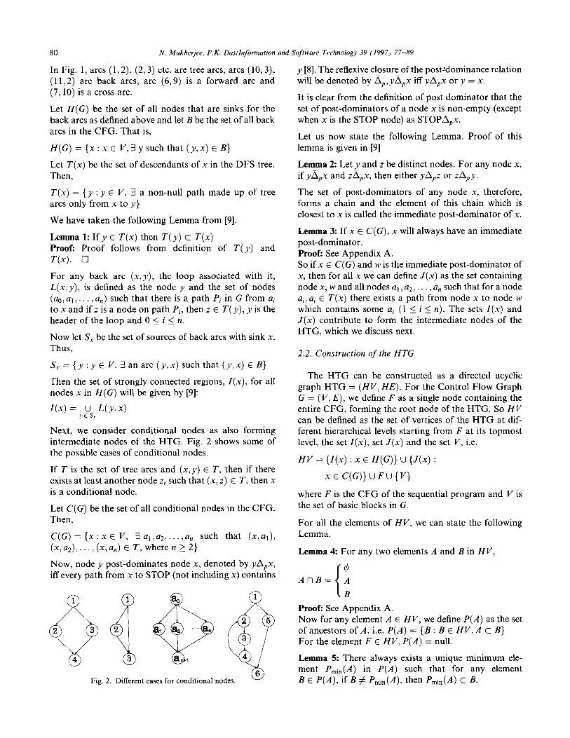
Next, we consider conditional nodes as also forming intermediate nodes of the HTG. Fig. 2 shows some of the possible cases of conditional nodes.

If T is the set of tree arcs and (x, y) E T, then if there exists at least another node z, such that (x, z) E T, then x is a conditional node.

Let C(G) be the set of all conditional nodes in the CFG. Then,

C(G) = {x : x E I/, 3 ulru2,. . . ,u, such that (~,a,),

(x, aI), . . . , (x, a,) E T, where n 2 2)

Now, node y post-dominates node x, denoted by yA,x, iff every path from x to STOP (not including x) contains

Fig. 2. Different cases for conditional nodes. Q9

y [8]. The reflexive closure of the post--dominance relation will be denoted by A*, yA,x iff yA,x or y = x.

It is clear from the definition of post dominator that the set of post-dominators of a node x is non-empty (except when x is the STOP node) as STOPA,x.

Let us now state the following Lemma. Proof of this

lemma is given in [9]

Lemma 2: Let y and z be distinct nodes. For any node x,

if yL\px and zA,x, then either yA,z or zA,y.

The set of post-dominators of any node x, therefore, forms a chain and the element of this chain which is closest to x is called the immediate post-dominator of x.

Lemma 3: If x E C(G), x will always have an immediate post-dominator. Proof: See Appendix A. So if x E C(G) and w is the immediate post-dominator of x, then for all x we can define J(x) as the set containing node x, w and all nodes al, u2,. . . , a, such that for a node Ui, ui E T(x) there exists a path from node x to node w which contains some Ui (1 5 i 5 n). The sets Z(x) and J(x) contribute to form the intermediate nodes of the HTG, which we discuss next.

2.2. Construction of the HTG

The HTG can be constructed as a directed acyclic graph HTG = (HV, HE). For the Control Flow Graph

G = (I’/, E), we define F as a single node containing the entire CFG, forming the root node of the HTG. So HI/ can be defined as the set of vertices of the HTG at different hierarchical levels starting from F at its topmost level, the set I(x), set J(x) and the set V, i.e.

HV = {Z(x) : x E H(G)} u {J(x) :

XE C(G)}uFu{L’}

where F is the CFG of the sequential program and V is the set of basic blocks in G.

For all the elements of HI/, we can state the following

Lemma.

Lemma 4: For any two elements A and B in HV,

1

4

AnB= A

B

Proof: See Appendix A. Now for any element A E HV, we define P(A) as the set of ancestors of A, i.e. P(A) = {B : B E HV, A C B}

For the element F E HV, P(A) = null.

Lemma 5: There always exists a unique minimum element P,i,(A) in P(A) such that for any element B E P(A), if B # Pmi”(A), then Pmi”(A) C B.

N. Mukherjee, P.K. Dasllnformation and Software Technology 39 (1997) 77-89 81

Proof: See Appendix A. For the element F, P(A) = null, hence Pmi”(A) = null. Each node of HT/ can be one of the following types:

a) Start node, b) Stop node, c) Simple node, d) Loop node, e) Conditional node, f) Compound node.

Next we start from the elements in V, i.e. the set of basic blocks, the start and stop nodes of the program. These nodes will form the leaf nodes of our HTG. Each basic block B will be connected to its immediate ancestor Pmi,(B). The arc e connecting Pmi” (B) with the node B is an element of HE and Pmin (B) is an element of HI/. Thus we shall obtain a set of intermediate nodes in the HTG which exist at the next upper level in the hierarchy. These intermediate nodes will be connected to their immediate ancestors which are also elements of HP’ by arcs which are elements of HE. Proceeding as above we shall ultimately reach the topmost level of the hierarchy, i.e. F the root node of the graph.

The next section describes how the user can assist the machine in choosing the most desirable form of parallelisation from the HTG so constructed.

3. User assisted parallelisation

In most of the traditional approaches of parallelisation (e.g. in [9]), extraction of functional parallelism and derivation of execution conditions are done automatically. The starting point is a predefined control flow graph. Task granularity is either fixed or adjusted automatically. However, automatic parallelisation of sequential codes derived in this manner may sometimes become too restrictive. The parallelisation is done depending on the control dependence and data dependence relations among the HTG nodes. Information about run-time data is clearly not available at compile time. Values of actual parameters in procedure calls, loop bounds and array subscripts should be estimated most conservatively by the compiler and this may lead to loss of exploitable parallelism.

In an interactive environment, we try to overcome these difficulties by allowing users to do the following:

1) 2)

3)

4)

choose the grain size according to their wish, ask the system to test the dependencies between any two chosen nodes, change the program by applying their domain knowledge so that dependencies are removed wherever possible, interact with the paralleliser and to obtain the information necessary to take actions described in 1,2, and 3.

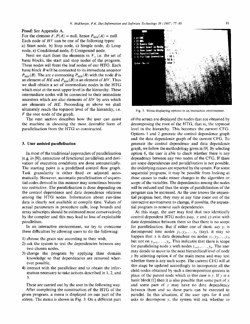
These are carried out by the user in the following way. After completing the construction of the HTG of the

given program, a menu is displayed on one part of the screen. The menu is shown in Fig. 3. On a different part

Fig. 3. Menu displaying options in an interactive environment.

of the screen are displayed the nodes that are obtained by decomposing the root of the HTG, that is, the topmost level in the hierarchy. This becomes the current CFG. Options 1 and 2 generate the control dependence graph and the data dependence graph of the current CFG. To generate the control dependence and data dependence graph, we follow the methodology given in [9]. By selecting option 6, the user is able to check whether there is any dependency between any two nodes of the CFG. If there are some dependencies and parallelisation is not possible, the underlying causes are reported by the system. For some

sequential programs, it may be possible from looking at these causes to make minor changes in the algorithm or scope of the variables. The dependencies among the nodes will be reduced and thus the scope of parallelisation of the program can be increased. As the user knows the sequential program best, they may at any time come out of the interactive environment to change, if possible, the sequential program to remove such dependencies.

At this stage, the user may find that two identically control-dependent HTG nodes (say, x and y) exist with data dependence between them so that there is no scope for parallelisation. But if either one of them, say y, is decomposed into nodes yl ,y2,. y,, (say), it may so happen that x is data dependent on nodes lyl ,y2,. . .J’~, butnotonyitl,..., yn. This indicates that there is scope for parallelising node x with nodes yi+, , . . , y,,. The user may decide to move to the next hierarchical level of node y by selecting option 4 of the main menu and may test whether there is any such scope. The current CFG will at this stage be updated accordingly to incorporate all the child nodes obtained by such a decomposition process in place of the parent node which in this case is y. If J‘ is a basic block [I] then it is also possible that some part of I and some part of y may have no data dependency between them and so these parts can be executed in parallel. In this situation, if the user opts for 4 and asks to decompose y, the system will ask whether to


split the basic block y. The user forces the system to split the basic block into two and consider them as two different nodes,

Option 5 helps the user to move to the previous hierarchical level, if there is any, either from any one node or from the entire Control Flow Graph and to update the current CFG accordingly.

Thus the user has the flexibility to move to different hierarchical levels of the HTG and to adjust the task granularity interactively. It is completely up to the discretion of the user to decide upon the starting CFG for dependency checking and parallelisation of the sequential code. The user can get a rough estimate of the execution time of any of these nodes as and when required. This serves to help the user in deciding whether to parallelise any two HTG nodes or whether to move to the next lower or upper level in the hierarchy. For example, it may not be desirable to execute in parallel those tasks that have very small execution times, because the overhead to run them in parallel on different processors may reduce the efficiency instead of increasing it. In all such situations the user may make the appropriate decision by obtaining the estimate of execution time.

Option 7 generates the parallel code of the sequential program. The basis is the current control flow graph and the CDG and DDG generated by the system. Again, the user decides which nodes of the CFG are to be parallelised and the execution conditions of these nodes are generated by the system. Details of the generation of execution conditions are discussed in the next section. The nodes are converted to parallel tasks to be run on different MIMD processors.

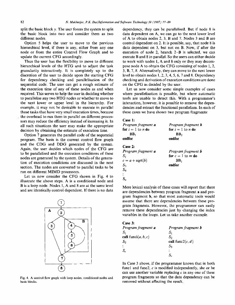
Let us now consider the CFG shown in Fig. 4 to illustrate the above steps. A is a conditional node and B is a loop node. Nodes 1, A and 8 are at the same level and are identically control dependent. If there is no data

Fig. 4. A control flow graph with loop nodes, conditional nodes and

basic blocks.

dependency, they can be parallelised. But if node 8 is data dependent on A, we can go to the next lower level of A to obtain nodes 2, 3, B and 7. Nodes 3 and B are control dependent on 2. It is possible, say, that node 8 is data dependent on 3, but not on B. Now, if after the execution of node 2, branch 2-B is selected, we can execute B and 8 in parallel. So the users can either decide to work with nodes 1, A and 8 only or they may decompose node A to obtain the CFG consisting of nodes 1,2, 3, B, 7, 8. Alternatively, they can move to the next lower level to obtain nodes 1,2, 3,4, 5,6, 7 and 8. Dependency checking and derivation of execution conditions are done on the CFG as decided by the user.

Let us now consider some simple examples of cases where parallelisation is possible, but where automatic tools are unable to detect this. With a programmer’s interaction, however, it is possible to remove the dependencies and extract the functional parallelism. In each of these cases we have shown two program fragments:

Case 1: Program fragment a for i = 1 to n do

BBI

Program fragment b for i = 1 to n do

BJ% endfor

Case 2: Program fragment a

Sl c = a + sqrt(b)

53

&

endfor

Program fragment b for c = 1 to m do

BBt endfor

Mere lexical analysis of these cases will report that there are dependencies between program fragment a and program fragment b, so that most automatic tools would assume that there are dependencies between these program fragments. However, the programmer can easily remove these dependencies just by changing the index variables in the loops. Let us take another example.

Case 3: Program fragment a

Sl

call funcl(a, b, c)

s2

i

Program fragment b

SI

s2

call func2(c, d)

s3

s,

In Case 3 above, if the programmer knows that in both funcl and func2, c is modified independently, she or he can use another variable replacing c in any one of these program fragments so that the data dependency can be removed without affecting the result.

Case 4: Program fragment a for i = p to q do

C(i) = a(i) + b(i)

N. Mukherjee. P.K. Dasllnformation and Software Technology 39 (1997) 77-89 83

Similarly in Case 4, if it is known to the user that there is Program fragment b no intersection between the range (p,q) and (m,n), the for k = m to n do user can inform the system about the possibility of

c(k) = max(a(k), b(k)) parallelising these two program fragments. Consider the following program fragments:

endfor endfor

begin fori=ltondo

read (first [il) endf or fori=ltondo

read (secondCi1) endf or for i = 1 to n do

read (thirdli] 1 endf or if (first CO] <second CO] and first CO1 <third CO1 )

begin process-block(first) if (second CO1 <third CO1 ) begin

process-block(second) process-blockcthird)

end else begin

process-block(third) process-block(second)

end end

else if (second[Ol Cf irst CO1 and second CO1 <third CO1 1

begin process-block (second) if (first [Ol <third CO1 1 begin

process-block(first) process-blockcthird)

end else begin

process-block(third) process-block(first)

end end

else begin

process-block(third) if (first CO1 <second [Ol ) begin

process-block(first) process-block(second)

end else

end

begin process-block(second) process-block(first)

end end

end

/* Start of node A */

/* BBo */ /*EndofnodeA*/ /* Start of node B */

/* BB, */ /* End of node B */ /* Start of node C */

/* BB2 */ /* End of node C */ /* Start of node F */

/* BB, */ /* Start of node D, */

/* start of BB4 */ /* End of BB, */

/* Start of BBS */ /* End of BBS */ /* End of node D, *

/* Start of node D, */

/* BB6 */ /* Start of node Dzl */

/*Start of BB, */ /* End of BB, */

/* Start of BBs */ /* End of BB, */ /* End of node Dsl */

/* BB, */ /* Start of node Dz2 */

/* Start of BBio */ /* End of BB,, */

/* Start of BB,, */ /* End of BB,, */ /* End of D,, */ /* End of node D2 */ /* End of node D */

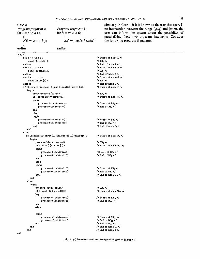
Fig. 5. (a) Source code of the program discussed in Example 1.

N. Mukherjee. P.K. Dasllnformation and Software Technology 39 (1997) 77-89

Fig. 5. (b) Control Flow Graph of the program shown in Fig. 5a

Program fragment a

SI s2

S3 : c = sqrt(b*b-a)

s4

S5

i

Program fragment b

if (c > x)

BBl else

BB2

Here, program fragment a is a basic block and b is a conditional node. There is data dependence between these two. But in a, variable c is last updated before S4. So if a is split up into two basic blocks, al and a2, the former containing statements S, to S3 and the latter containing statements S4, S5,. , S,, then a2 and node b can be executed in parallel. Whether to split a block or not is decided by the user in the interactive environment. The user also decides where to split a block. If the user decides to split any basic block, the node representing that basic block in the CFG will be replaced by two new nodes and dependency analysis will be done on this newly formed CFG.

4. Deriving execution conditions

We shall now formalise the notion of execution conditions. We shall use literals like x,Y, al,a2 etc. to represent nodes, and notations such as x-y, al-b, etc. to represent arcs of the CFG.

4.1. Control dependence conditions

The control dependence conditions for a node x are derived from the CDG. If x is a node in the CDG which is control dependent on al, a2,. . . a,, with labels al-b,,

a2-bz, .. . , an-b, respectively, then the control condition for x is:

al-b, V a2-b2 V . . . V an-b,

4.2. Data dependence conditions

Before deriving data dependence conditions, we define the following. For any two nodes x and Y, x6rY denotes that the node Y is control dependent on node x and xS,y denotes the transitive closure of xS,Y. Then, for any node x, RN(x) is the set of nodes reachable from node x in the CDG.

RN(x) = {Y I Xh,‘Y)

For any arc x-y, RB(x-y) is the set of nodes reachable following the path x-y in the CDG.

,,i;-Y) = {z 13 a such that xS,a with label x-y and

c

Now for any two nodes x and y, Exe,(x) is the set of all branches in CFG whose traversal executes x but bypasses the execution of y.

Exe,(x) = {p-q\ y E RN(p) and y $RB(p-q) and x E

RB(p-q))

Lemma 6a: If a-b E Exe,(x), then if a-b is true, x will be

executed, but not y. Proof follows from definition.

Lemma 6b: If x is executed, but not y, then at least one label of Exe,(x) is true. We can now derive the data dependent condition for any

node x. If node x is data dependent on node Y, then x can be executed only when y has completed its execution, or when some path in the CFG has been selected so that x will be executed but Y will not be executed at all. So the data dependent condition for node x dependent on nodes cl, c2, c3,. . , c, will be given by:

(cl V Exe,,(x)) A (c2 V Exec2(x)) A.. . A (c, V Exec,(x))

5. Examples

In this section we consider the Control Flow Graphs of


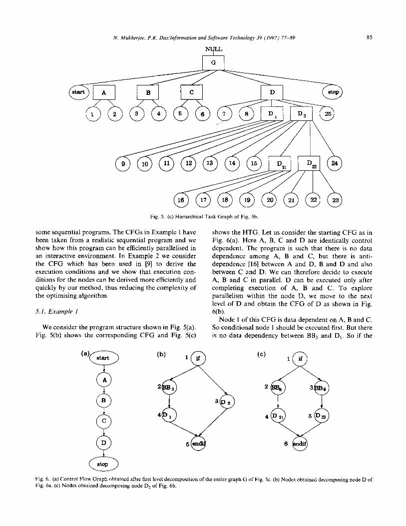
Fig. 5. (c) Hierarchical Task Graph of Fig. Sb.

some sequential programs. The CFGs in Example 1 have been taken from a realistic sequential program and we show how this program can be efficiently parallelised in an interactive environment. In Example 2 we consider the CFG which has been used in [9] to derive the execution conditions and we show that execution conditions for the nodes can be derived more efficiently and quickly by our method, thus reducing the complexity of the optimising algorithm.

5.1. Example I

We consider the program structure shown in Fig. 5(a). Fig. 5(b) shows the corresponding CFG and Fig. 5(c)

(a) start

F A

0 B

0 C

D

8 stop

shows the HTG. Let us consider the starting CFG as in Fig. 6(a). Here A, B, C and D are identically control dependent. The program is such that there is no data dependence among A, B and C, but there is anti- dependence [16] between A and D, B and D and also between C and D. We can therefore decide to execute A, B and C in parallel. D can be executed only after completing execution of A, B and C. To explore parallelism within the node D, we move to the next level of D and obtain the CFG of D as shown in Fig.

6(b). Node 1 of this CFG is data dependent on A, B and C.

So conditional node 1 should be executed first. But there is no data dependency between BB3 and Dr. So if the

(cl

2

Fig. 6. (a) Control Flow Graph obtained after first level decomposition of the entire graph G of Fig. 5c. (b) Nodes obtained decomposing node D of

Fig. 6a. (c) Nodes obtained decomposing node Dz of Fig. 6b.


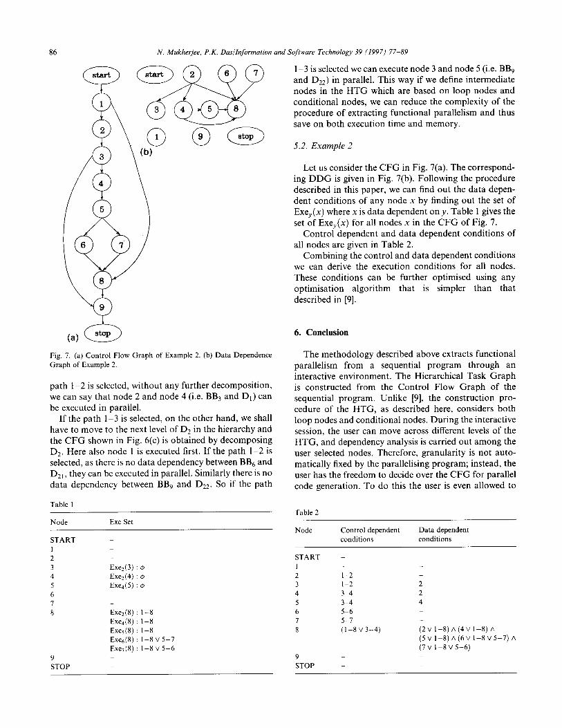
Fig. 7. (a) Control Flow Graph of Example 2. (b) Data Dependence Graph of Example 2.

path l-2 is selected, without any further decomposition, we can say that node 2 and node 4 (i.e. BBs and D,) can be executed in parallel.

If the path l-3 is selected, on the other hand, we shall have to move to the next level of Dz in the hierarchy and the CFG shown in Fig. 6(c) is obtained by decomposing Dz. Here also node 1 is executed first. If the path l-2 is selected, as there is no data dependency between BB6 and Dzl, they can be executed in parallel. Similarly there is no data dependency between BBg and D12. So if the path

Table 1

Node Exe Set

START

9 STOP

_

Exe2(3) Exd4) E%(5)

_

E%(8) E%(8) Ew(8) Exe&) Exe-i@)

1-8 l-8 1-8 1-8~5-7 1-8~5-6

l-3 is selected we can execute node 3 and node 5 (i.e. BBs and Dz2) in parallel. This way if we define intermediate nodes in the HTG which are based on loop nodes and conditional nodes, we can reduce the complexity of the procedure of extracting functional parallelism and thus save on both execution time and memory.

5.2. Example 2

Let us consider the CFG in Fig. 7(a). The corresponding DDG is given in Fig. 7(b). Following the procedure described in this paper, we can find out the data dependent conditions of any node x by finding out the set of Exe,(x) where x is data dependent on y. Table 1 gives the set of Exe,(x) for all nodes x in the CFG of Fig. 7.

Control dependent and data dependent conditions of all nodes are given in Table 2.

Combining the control and data dependent conditions we can derive the execution conditions for all nodes. These conditions can be further optimised using any optimisation algorithm that is simpler than that described in [9].

6. Conclusion

The methodology described above extracts functional parallelism from a sequential program through an interactive environment. The Hierarchical Task Graph is constructed from the Control Flow Graph of the sequential program. Unlike [9], the construction procedure of the HTG, as described here, considers both loop nodes and conditional nodes. During the interactive session, the user can move across different levels of the HTG, and dependency analysis is carried out among the user selected nodes. Therefore, granularity is not automatically fixed by the parallelising program; instead, the user has the freedom to decide over the CFG for parallel code generation. To do this the user is even allowed to

Table 2

Node Control dependent conditions

Data dependent conditions

START ~ 1 _ 2 1-2 3 l-2 4 3-4 5 3-4 6 5-6 7 5-7 8 (1-8~3-4)

9 STOP

_ _ _

2 2 4

_

(2 v l-8) A (4v l-8) A (5vl-8)~(6vl-8~5%7)A (7 v l-8 v 5-6) _ _

N. Mukherjee, P.K. Dasllnformation and Software Technology 39 (1997) 77-89 87

cross basic block boundaries, if required, to increase the scope of parallelisation. The derivation of execution condition is also done in this paper in such a way that one can arrive at a nearly optimal set of execution conditions and the subsequent optimisation process can therefore be simplified.

6.1. Scope of further work

In this paper, we have considered only functional parallelism. Further work can be done to incorporate loop level parallelism in this approach. As for example in Fig. 4, if node 8 is data dependent on node 4, and if it is an anti-dependence, 8 can be executed in parallel with node 5 (provided no dependence relation exists between nodes 5 and 8) only during the last execution of the loop. This type of problem can be solved if we analyse both functional and loop level parallelism in the same approach.

The system generates parallel tasks to be executed on loosely coupled MIMD machines, for example on a net- work of transputers, that establish a message passing environment among the processors. Under this environment, even if two tasks have data dependency between them, they can be executed in parallel provided one sends the modified values of the shared variables to the other task and the latter uses the variables in such a way that the result becomes identical to the result of the sequential execution. How and when this message will be passed can be decided during the interactive session for the extraction of parallelism.

Subroutines are very important in sequential programs developed with a modular approach. We have considered subroutines as compound nodes which consist of other nodes and thus have structures similar to the HTG. We treat each of these compound nodes, representing a subroutine, as a separate HTG and try to extract parallelism within that node only. But the nodes of any subroutine can also be executed in parallel with nodes in the main program or with nodes of other subroutines. If we treat each compound node separately, such possibilities cannot obviously be exploited. If we want to extract parallelism among different subroutines and between subroutines and the main program, we shall have to form composite HTGs for all possible combi- nations of main program and subroutines. This increases the complexity of the analysis to almost a formidable extent for any non-trivial program. An effective solution of this problem calls for further work and the problem

has not been addressed in this paper. One of the remaining limitations of the present work is

that while the user may be able to predict some behaviour of the runtime environment and may help the compiler to collect some information which is not apparent from the sequential program code, it is not possible for a user to predict all possible runtime

behaviours. If the compiler tries to solve the parallelising problem statically, the solution will always be conservative and we will not be able to utilise the scope of

parallelisation of a sequential program to the fullest extent. To overcome this, a method needs to be worked out to tackle the problem dynamically at run-time, possibly with help from the operating system.

Appendix A

Lemma 3: If x E C(G), x will always have an immediate

post-dominator. Proof: If x is the STOP node, then x does not have any outgoing arcs. So x 4 C(G).

If x is not the STOP node, then the set of post- dominators of x is non-empty as STOPA,x. So the set of post-dominators of x will form a chain, and the element of the chain which is closest to x will be the immediate post-dominator of x. If the chain contains only the node STOP, then STOP will be the immediate post-dominator of x. Hence proved. Cl

Lemma 4: For any two elements A and B in HV,

Proof: The lemma is true if either A or B is F and it is also true if either A E V or B E V or A, B E V. So the other non-trivial cases are as follows:

a) A = Z(x) and B= Z(y)

b) A = Z(x) and B = J(y)

c) A = J(x) and B = J(y)

Case A If A = Z(x) and B = Z(y),

then,

A =Z(x) =,.JJ. )i

L(P,x) andB=Z(y) =yys,Z4q,y) ,

Now, if Z(x) n Z(v) is non-empty, let z E Z(x) f~ Z(y), then there exist two loops L(p;, x) and L(q;, y), such that z E L(pi, X) and z E L(qi,y).

By definition, there exists a tree path Pi from x to z and

there exists another tree path P2 from y to z. So we get two tree paths from two distinct nodes x and y, to z. But a node can have only one incoming tree arc. So the above situation is possible only if either y is on PI or x is on Pz. Let us assume y is on Pt. Then y E T(x). By Lemma 1, T(y) c T(x). Loop L(pi, x) has only a single entry point. SO qi also belongs to L(pi, x), otherwise the back arc (qi, x) will be another entry point of the loop which is not possible. By similar reasoning, all nodes belonging to the loop L(qi,v) also belong to the loop

88 N. Mukherjee, P.K. Dasjlnfortnation and Software Technology 39 (1997) 77-89

L( pi, x). SO L(qi, y) c L(pi, X) and hence Z(y) c Z(X).

Similarly, if x is on Pz, we can prove that L( pi> X) C L(qi, y) and SO we can say Z(x) C Z(y). Thus if Z(x) n Z(y) is non-empty, then either Z(y) c Z(x) or Z(x) c Z(y).

Case B If A=Z(x) and B=J(y), let ZEZ(x)nJ(y). So z E Z(x) and also z E J(y).

Let

Z(X) =,ys L(P,x) and z E L(pi,x). r

Then there exists a path PI from x to z and a path P2 from y to z. As there cannot be another entry for loop L(pj, x), either x is on P2 or y is on PI Let w be the immediate post dominator of y. Then all paths from y to STOP contain w. Let us assume x is on Pz. For reducible graphs, there cannot be any forward jump from outside to the middle of the loop. So there cannot be any other path P3 which does not contain x, but contains any other nodes of L(pi, x). So there exists a path P from y to w which contains x and Pi and w post-dominates all nodes belonging to Z( pi, x). This proves that L( pi, x) c J(y) and so Z(x) c J(y). If y is on P,, Pi post-dominates all nodes in the loop and so it also post-dominates y. Therefore, either w = pi or w E L(pi,x). This proves that J(y) C Z(X).

Case C If A = J(x) and B = J(y) and J(x) n J(y) is non-empty, let us assume that z is any node which belongs to J(x) n .Z( y). So z E J(x) and z E J(y). Let p be the immediate post dominator of x and q be the immediate post dominator of y. Consider a path PI from z to p and another path P2 from z to q. If these two paths are distinct, then there exists a path from x to q through z. So there is a path from x to STOP which does not contain p. This contradicts the fact that p is the post dominator of x. So either p is on P2 or q is on PI. Similarly there are two paths P3 and P4 from x to z and from y to z. But, z E T(x) and z E T(y). This is not possible if P3 and P4 are distinct. So either x is on P4 or y is on P3. Hence we prove that, either J(x) c J(y) or

J(Y) c J(x). 0

Lemma 5: There always exists a unique minimum element P,i,(A) in P(A) such that for any element B E P(A), if B # P,i”(A), then Pmi,(A) C B. Proof: Let C E P(A) and D E P(A).

SoC~HVandD~HVandctlD#@ From lemma 4, either C C D or D c C. This is true for all elements of P(A). So there exists a unique minimum element Pmi”(A). 0

Appendix B

B.l. Control Dependence Graph

For any two nodes x and y, we can say xS,y, i.e. y is control dependent on node x with label x-a where (x, a) is an arc in CFG, iff

1. y does not post dominate x and 2. There exists a non-null path P = (x, a,. . . , y), such

that for any z on this path P (excluding x and y), y post dominates z.

The Control Dependence Graph of a CFG (whose set of vertices is denoted by V) is defined as the directed graph with labelled arcs, CDG = (CV, CE) such that CV = V and (x, y) E CE withe label x-a iff xS,y with label x-a.

B.2. Data Dependence Graph

Between any two nodes x and y in a CFG, the following three relations can occur:

a) y is reachable from x, b) x is reachable from y c) x is not reachable from y, and y is not reachable from

X.

Now x and y can share a common memory location and if at least one of them performs a write operation while accessing that memory location, we say a conflict has occurred. If y is reachable from x and a conflict occurs, then y is data dependent on x (xbdy). If x is reachable from y and a conflict occurs, then x is data dependent on y ( ybdx). But in the third case, i.e. x is not reachable from y and y is not reachable from x, any such conflict can be ignored and there is no question of data dependency. The Data Dependence Graph DDG = (DV, DE) of a CFG (with vertex, set V) can be defined as follows: DV = V and (x,y) E DE is xbdy.

References

PI

121

[31

[41

151

161

R. Allen and K. Kennedy, Automatic translation of FORTRAN

programs to vector form, ACM Trans. on Programming

Languages and Systems (October 1987) 491-542.

R. Cytron, M. Hind and W. Hsieh, Automatic generation of DAG

parallelism, In Proc. 1989 SIGPLAN Conf. on Programming

Language Design and Implementation, July 1989, pp. 54468.

M. Girkar and C.D. Polychronopoulos, Automatic extraction of functional parallelism from ordinary programs, IEEE Trans. on

Parallel and Distributed Systems (March 1992) 1666178.

C. Koelbel and P. Mehrotra, Compiling global name space

parallel loops for distributed execution, IEEE Trans. on Parallel and Distributed Systems (October 1991).

K. Kennedy, K.S. McKinley and C. Tseng, Interactive Parallel

Programming Using the Parascope Editor. IEEE Trans. on

Parallel and Distributed Systems (July 1991) 329-341.

D.J. Lilja, Exploiting the parallelism available in loops, Computer

(February 1994) 13-26.


[7] A. Rogers and K. Pingali, Compiling for distributed memory

architectures, IEEE Trans. on Parallel and Distributed Systems

(March 1994) 281-298.

[S] J. Ferrante, K.J. Ottenstein and J.D. Warren, The program

dependence graph and its use in optimization, ACM Trans. on

Programming Languages and Systems (July 1987) 319-349.

[9] M. Girkar, Functional parallelism: theoretical foundations and

implementation, Ph.D. Thesis, University of Illinois at Urbana-

Champaign, 1992.

[IO] M. Girkar and C.D. Polychronopoulos, The Hierarchical Task

Graph (HTG): The soul of a parallehzing compiler, Technical

Report, Center for Supercomputing Research and Development,

University of Illinois, October 1990.

[I l] A.V. Aho, R. Sethi and J.D. Ullman, Compilers: Principles,

techniques and tools, Addison Wesley, Reading, MA, March

1986.

[12] V. Sarkar, Partitioning and scheduling parallel programs for

execution on multiprocess, Ph.D. Thesis, Computer Systems

Laboratory, Dept of Electrical Eng. and Comp. Sci., Stanford

University, April 1987.

[ 131 R.E. Tarjan, Testing flow graph reducibility, Journal of Computer

and System Sciences (December 1974) 3555365.

[I41 J.T. Schwartz and M. Sharir, A design for optimizations of the

bivectoring class, Technical Report, Courant Institute of

Mathematical Sciences, New York University, September 1979.

[15] M. Hecht, Flow analysis of computer programs, Elsevier North-

Holland, New York, 1977.

[16] M.J. Wolfe, Optimizing supercompilers for supercomputers, The

MIT Press, Cambridge, MA, 1989.

[17] Puranjan Mukhopadhyay, On the automatic parallelisation of

imperative language programs for distributed memory machines,

M.C.S.E. Thesis, Jadavpur University, 1993.

[18] C.D. Polychronopoulos, Auto scheduling: control flow and data

flow come together, Technical Report, Center for Supercomputing

Research and Development, University of Illinois, December 1990.

an approach towards parallelisation of sequential programs in an interactive environment

Documents