An application of seismic attributes analysis for mappingof gas bearing sand zones in the sawan gas field, Pakistan

Tahir Azeem1• Wang Yanchun1 • Perveiz Khalid2 •

Liu Xueqing1 • Fang Yuan1 • Cheng Lifang1

Received: 3 April 2015 / Accepted: 7 December 2015 / Published online: 21 December 2015� Akademiai Kiado 2015

Abstract Sandstone intervals of the Lower Goru Formation of the Cretaceous age are

proven reservoir intervals in the middle Indus Basin, Pakistan. However, based on seismic

data interpretation, it is difficult to differentiate payable gas sand from non-payable gas

sand. Various types of post-stacks seismic attributes are extracted and analyzed to dif-

ferentiate payable gas sand from non-payable. The analysis reveals that average instan-

taneous frequency, peak spectral frequency, average instantaneous phase and sweetness

seem to be more effective attributes along with energy half time. Sweetness attribute map

shows two sweet spot below the targeted window which indicate to the presence of gas

play. Statistical analysis is also carried out to find the associations between seismic

attributes and thickness of gas layer values. Cross plots of these attributes were quantified

through regression analysis. A good correlation with regression coefficient (R2)[ 0.78 is

found between seismic attributes and gas layer thickness except average instantaneous

phase attribute, which lays the foundation for predicting the thickness of gas reservoir.

Keywords Post-stack attributes � Statistical analysis � Sawan gas field � Gas layer

thickness � Gas bearing sand zones

1 Introduction

Discrimination of hydrocarbon sand intervals from non-hydrocarbon sands can easily

possible from the interpretation of seismic data (Dobrin and Savit 1988; El-Mowafy and

Marfurt 2008; Khalid et al. 2014a). However, it is difficult to distinguish payable hydro-

carbon interval from non-payable interval by the interpretation of seismic data only

& Tahir Azeemtahir2rd@yahoo.com

1 China University of Geosciences, Beijing 100083, China

2 Institute of Geology, University of the Punjab, Lahore 54590, Pakistan

123

Acta Geod Geophys (2016) 51:723–744DOI 10.1007/s40328-015-0155-z

(Khalid and Ghazi 2013). For this purpose, various techniques and methods are in practice

(Marfurt et al. 1998; Fu et al. 2006; Khalid et al. 2014b). The sand intervals of the Lower

Goru Formation of the Cretaceous age are producing oil and gas in various parts of Lower,

Middle and Upper Indus basin of Pakistan. However, in Swan gas field (26.80�–27.40�N,

68.70�–69.40�E) in the Middle Indus basin, several wells drilled in these sand intervals,

declared dry or abandoned. These wells were drilled in these intervals based on structural

interpretation of seismic data. However, based on this qualitative interpretation, we were

unable to differentiate between payable and non-payable sand intervals. The quantitative

analysis of seismic amplitude anomalies was not considered. In this work, an attempt is

made to resolve seismic amplitudes related problems through seismic attribute analysis as

suggested by Taner et al. (1979).

Among various seismic techniques, seismic attributes is a powerful tool, which can be

utilized to interpret pore fluid saturation and type at in situ conditions (Marfurt et al. 1998).

According to application various researchers have been classified the seismic attributes into

different categories. Taner et al. (1994) has divided seismic attributes into geometrical and

physical attributes. Physical attributes are closely linked with lithology, change in deposi-

tional environments and pore fluid properties. These attributes are commonly used to predict

the reservoir properties of the targeted interval (Bodine 1984, 1986; Taner 2001; Løseth

et al. 2009; Raef et al. 2015). With the advent of digital recording the quality of seismic

amplitude data has been tremendously improved (Chopra and Marfurt 2005). Seismic

amplitude is used as principal parameter to determine the physical properties of rock-fluid

composite, as the strong amplitudes (bright spots) have a good correlation with lithology,

pore fluid properties and edges of hydrocarbon-water interfaces (Bodine 1984, 1986; Taner

2001; Chopra and Marfurt 2005). However, when the thickness of the reservoir interval is

very close to seismic resolution limit then, the reflected signals from the top and bottom of

the layers undergo constructive or destructive interference which, causes to produce a single

event of high amplitude (Widess 1973; Robertson and Nogami 1984; Chung and Lawton

1995). Such kinds of events create ambiguity and make it difficult to distinguish the pro-

ductive and non-productive sand through conventional amplitude analysis (Rana et al.

2006). Therefore, to improve the reservoir analysis, in addition to amplitude attributes other

seismic attributes such as sweetness, average instantaneous phase, average instantaneous

frequency and spectral frequency etc. are in practice (Horkowitz and Davis 1996; Taner

2001; Rana et al. 2006; Hart 2008; Ye et al. 2008; Raef et al. 2015). Sweetness is commonly

used to identify the sand, shale, sandstones and channel sand and also helpful to check the

lateral as well as vertical continuity of the targeted interval (Hart 2008; Ahmad and Rowell

2012; Wang et al. 2012). Post stack attributes like RMS amplitude, maximum peak

amplitude, maximum trough amplitude, average instantaneous frequency, average instan-

taneous phase and relative impedance have good relation with the lateral variation of the

reservoir, while reflection intensity, peak spectral frequency attributes are sensitive to

reservoir thickness (Marfurt and Kirlin 2001; Taner 2001; Gholami et al. 2014).

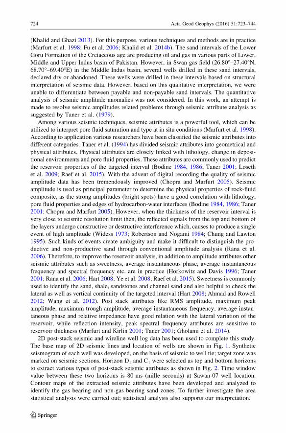
2D post-stack seismic and wireline well log data has been used to complete this study.

The base map of 2D seismic lines and location of wells are shown in Fig. 1. Synthetic

seismogram of each well was developed, on the basis of seismic to well tie; target zone was

marked on seismic sections. Horizon D1 and C1 were selected as top and bottom horizons

to extract various types of post-stack seismic attributes as shown in Fig. 2. Time window

value between these two horizons is 80 ms (mille seconds) at Sawan-07 well location.

Contour maps of the extracted seismic attributes have been developed and analyzed to

identify the gas bearing and non-gas bearing sand zones. To further investigate the area

statistical analysis were carried out; statistical analysis also supports our interpretation.

724 Acta Geod Geophys (2016) 51:723–744

123

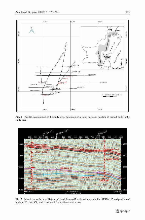
Fig. 2 Seismic to wells tie of Gajwaro-01 and Sawan-07 wells with seismic line SPSM-115 and position ofhorizons D1 and C1, which are used for attributes extraction

Fig. 1 (Inset) Location map of the study area. Base map of seismic lines and position of drilled wells in thestudy area

Acta Geod Geophys (2016) 51:723–744 725

123

1.1 Geology of the area

The study area is a part of the Middle Indus Basin, which is bounded by Sargodha High in the

north, Jacobabad and Mari-Kandkot Highs (collectively called Sukkur Rift) in the south. The

eastern boundary is marked by the Indian Shield and the western boundary is marked by

Kirthar and Suleiman Fold and Thrust Belt (Kadri 1995). Structural configuration of this area

is the direct result of three post-rifting tectonic events: late Cretaceous uplifting and erosion,

basement rooted NW–SE oriented wrench faults and late Tertiary to recent uplifting of

Jacobabad and Khairpur High (Ahmad et al. 2004). These Highs (Jacobabad and Khairpur)

play an important role to form the structural and stratigraphic traps in the Kadanwari and

Sawan areas (Ahmad et al. 2004; Berger et al. 2009). In the study area, the uplifting of

Khairpur High positioned the Lower Goru sequence such as, reservoir quality sand of

proximal depositional system are positioned into structurally deep areas whereas, non-

reservoir quality distal parts are positioned updip to form the traps (Berger et al. 2009).

The organic rich black shales of Cretaceous ages are the proven source rock in the

Middle and Lower Indus Basin which, are mainly composed of shale with subordinate

amounts of black siltstone, sandstone and nodular argillaceous limestone (Kadri 1995). The

Formation was deposited in the marine environments at the western passive margin of the

Indian plate. Thickness of the Sembar Formation ranges from 0 to more than 260 m (Iqbal

and Shah 1980). The Sembar Formation is deeply buried and thermally mature towards the

western edge of the Indus basin and becomes shallower and less mature towards the eastern

edge (Wandrey et al. 2004). The Sembar Formation is overlain by the Lower Goru For-

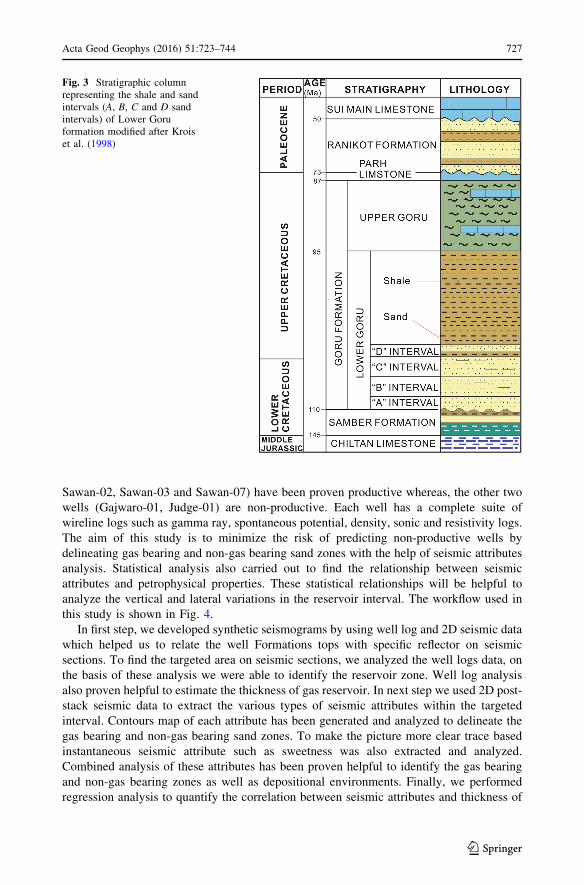
mation, which is the proven reservoir rock in the study area. The upper part of the Lower

Goru is mainly composed of shale whereas the lower part is mainly composed of medium

to coarse grained sandstones with thin layers of shale and limestone. The lower portion of

this reservoir character sandstones is further divided into A, B, C and D sand intervals

(Fig. 3) (Krois et al. 1998). Deposition of these reservoir intervals took place in deltaic,

shallow marine environments during lowstand phase; when detached medium to coarse

grained sediments were deposited on top of the distal (shale and siltstone) sediments of the

previous highstand systems tract (Berger et al. 2009). Petrographically, A and B intervals

can be classified as quartz arenites (Berger et al. 2009) whereas, C interval includes

significant amount of partially altered volcanic rock fragments and pore lining iron chlorite

cement due to which, the sands of this interval can be classified as sublith to lithic arenites

(McPhee and Enzendorfer 2004; Berger et al. 2009). Sands of B and C intervals are the

main reservoirs in the study area (Munir et al. 2011) and show high porosities (average

absolute porosities 16 %) and permeabilities between the depths of 3000–3500 m. This

reservoir interval of the Lower Goru Formation is directly overlain by transgressive shales

and siltstones of the Upper Goru Formation, which act as regional seal in the Middle and

Lower Indus basin (Berger et al. 2009).

2 Methodology

The proper identification of hydrocarbon bearing reservoir zones based on 2D seismic data

analysis has always been a very challenging task. In the study area, the thickness of

reservoir sandstone intervals at some places is very close to seismic resolution limit, which

make it difficult to differentiate productive and non-productive reservoir intervals. In this

study, we used wireline logs of six wells (Fig. 1), out of which four wells (Sawan-01,

726 Acta Geod Geophys (2016) 51:723–744

123

Sawan-02, Sawan-03 and Sawan-07) have been proven productive whereas, the other two

wells (Gajwaro-01, Judge-01) are non-productive. Each well has a complete suite of

wireline logs such as gamma ray, spontaneous potential, density, sonic and resistivity logs.

The aim of this study is to minimize the risk of predicting non-productive wells by

delineating gas bearing and non-gas bearing sand zones with the help of seismic attributes

analysis. Statistical analysis also carried out to find the relationship between seismic

attributes and petrophysical properties. These statistical relationships will be helpful to

analyze the vertical and lateral variations in the reservoir interval. The workflow used in

this study is shown in Fig. 4.

In first step, we developed synthetic seismograms by using well log and 2D seismic data

which helped us to relate the well Formations tops with specific reflector on seismic

sections. To find the targeted area on seismic sections, we analyzed the well logs data, on

the basis of these analysis we were able to identify the reservoir zone. Well log analysis

also proven helpful to estimate the thickness of gas reservoir. In next step we used 2D post-

stack seismic data to extract the various types of seismic attributes within the targeted

interval. Contours map of each attribute has been generated and analyzed to delineate the

gas bearing and non-gas bearing sand zones. To make the picture more clear trace based

instantaneous seismic attribute such as sweetness was also extracted and analyzed.

Combined analysis of these attributes has been proven helpful to identify the gas bearing

and non-gas bearing zones as well as depositional environments. Finally, we performed

regression analysis to quantify the correlation between seismic attributes and thickness of

Fig. 3 Stratigraphic columnrepresenting the shale and sandintervals (A, B, C and D sandintervals) of Lower Goruformation modified after Kroiset al. (1998)

Acta Geod Geophys (2016) 51:723–744 727

123

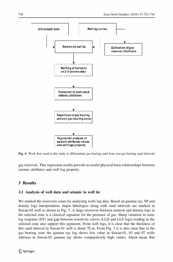
gas reservoir. This regression results provide us useful physical basis relationships between

seismic attributes and well log property.

3 Results

3.1 Analysis of well data and seismic to well tie

We marked the reservoirs zones by analyzing wells log data. Based on gamma ray, SP and

density logs interpretation, major lithologies along with sand intervals are marked in

Sawan-01 well as shown in Fig. 5. A large crossover between neutron and density logs in

the selected zone is a classical signature for the presence of gas. Sharp variation in sonic

log response (DT) and gap between resistivity curves (LLD and LLS logs) reading in the

selected zone also support this argument. From well logs, it is clear that the thickness of

this sand interval in Sawan-01 well is about 70 m. From Fig. 5 it is also clear that in the

gas bearing zone the gamma ray log shows low value in Sawan-01, 03 and 07 wells

whereas in Sawan-02 gamma ray shows comparatively high values, which mean that

Fig. 4 Work flow used in this study to differentiate gas bearing sand from non-gas bearing sand intervals

728 Acta Geod Geophys (2016) 51:723–744

123

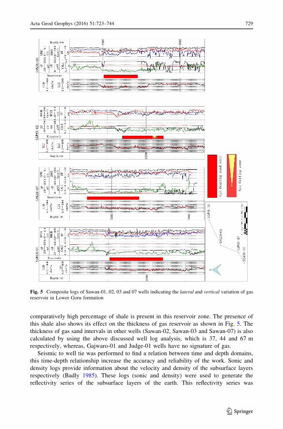
comparatively high percentage of shale is present in this reservoir zone. The presence of

this shale also shows its effect on the thickness of gas reservoir as shown in Fig. 5. The

thickness of gas sand intervals in other wells (Sawan-02, Sawan-03 and Sawan-07) is also

calculated by using the above discussed well log analysis, which is 37, 44 and 67 m

respectively, whereas, Gajwaro-01 and Judge-01 wells have no signature of gas.

Seismic to well tie was performed to find a relation between time and depth domains,

this time-depth relationship increase the accuracy and reliability of the work. Sonic and

density logs provide information about the velocity and density of the subsurface layers

respectively (Badly 1985). These logs (sonic and density) were used to generate the

reflectivity series of the subsurface layers of the earth. This reflectivity series was

Fig. 5 Composite logs of Sawan-01, 02, 03 and 07 wells indicating the lateral and vertical variation of gasreservoir in Lower Goru formation

Acta Geod Geophys (2016) 51:723–744 729

123

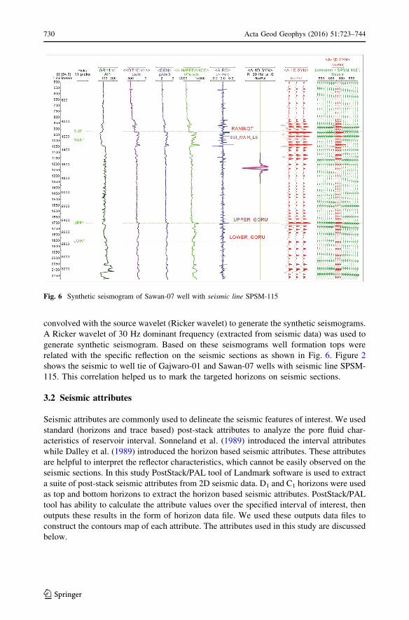
convolved with the source wavelet (Ricker wavelet) to generate the synthetic seismograms.

A Ricker wavelet of 30 Hz dominant frequency (extracted from seismic data) was used to

generate synthetic seismogram. Based on these seismograms well formation tops were

related with the specific reflection on the seismic sections as shown in Fig. 6. Figure 2

shows the seismic to well tie of Gajwaro-01 and Sawan-07 wells with seismic line SPSM-

115. This correlation helped us to mark the targeted horizons on seismic sections.

3.2 Seismic attributes

Seismic attributes are commonly used to delineate the seismic features of interest. We used

standard (horizons and trace based) post-stack attributes to analyze the pore fluid char-

acteristics of reservoir interval. Sonneland et al. (1989) introduced the interval attributes

while Dalley et al. (1989) introduced the horizon based seismic attributes. These attributes

are helpful to interpret the reflector characteristics, which cannot be easily observed on the

seismic sections. In this study PostStack/PAL tool of Landmark software is used to extract

a suite of post-stack seismic attributes from 2D seismic data. D1 and C1 horizons were used

as top and bottom horizons to extract the horizon based seismic attributes. PostStack/PAL

tool has ability to calculate the attribute values over the specified interval of interest, then

outputs these results in the form of horizon data file. We used these outputs data files to

construct the contours map of each attribute. The attributes used in this study are discussed

below.

Fig. 6 Synthetic seismogram of Sawan-07 well with seismic line SPSM-115

730 Acta Geod Geophys (2016) 51:723–744

123

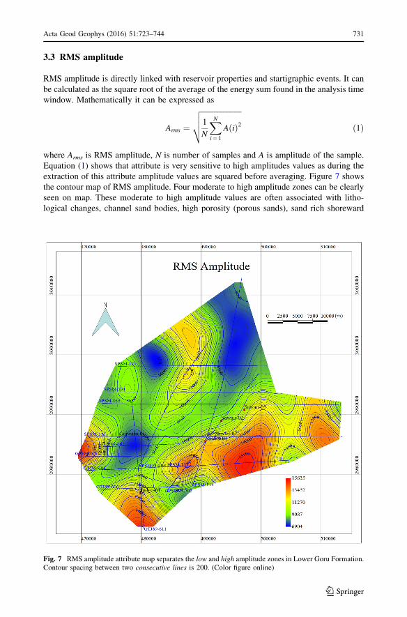
3.3 RMS amplitude

RMS amplitude is directly linked with reservoir properties and startigraphic events. It can

be calculated as the square root of the average of the energy sum found in the analysis time

window. Mathematically it can be expressed as

Arms ¼

ffiffiffiffiffiffiffiffiffiffiffiffiffiffiffiffiffiffiffiffiffiffi

1

N

X

N

i¼ 1

AðiÞ2

v

u

u

t ð1Þ

where Arms is RMS amplitude, N is number of samples and A is amplitude of the sample.

Equation (1) shows that attribute is very sensitive to high amplitudes values as during the

extraction of this attribute amplitude values are squared before averaging. Figure 7 shows

the contour map of RMS amplitude. Four moderate to high amplitude zones can be clearly

seen on map. These moderate to high amplitude values are often associated with litho-

logical changes, channel sand bodies, high porosity (porous sands), sand rich shoreward

Fig. 7 RMS amplitude attribute map separates the low and high amplitude zones in Lower Goru Formation.Contour spacing between two consecutive lines is 200. (Color figure online)

Acta Geod Geophys (2016) 51:723–744 731

123

facies, bright spots and especially gas saturated sand zones (Taner et al. 1979; Yushuang

and Simiao 2013). Whereas low amplitudes values may indicate that these zones contain

sandyshale, pro-delta or abyssal plain facies and not favorable for gas potential.

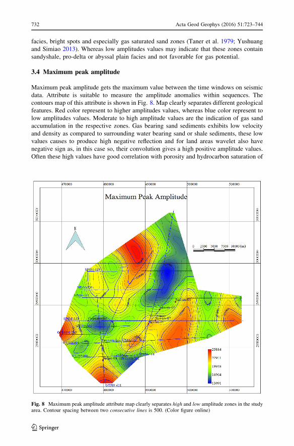
3.4 Maximum peak amplitude

Maximum peak amplitude gets the maximum value between the time windows on seismic

data. Attribute is suitable to measure the amplitude anomalies within sequences. The

contours map of this attribute is shown in Fig. 8. Map clearly separates different geological

features. Red color represent to higher amplitudes values, whereas blue color represent to

low amplitudes values. Moderate to high amplitude values are the indication of gas sand

accumulation in the respective zones. Gas bearing sand sediments exhibits low velocity

and density as compared to surrounding water bearing sand or shale sediments, these low

values causes to produce high negative reflection and for land areas wavelet also have

negative sign as, in this case so, their convolution gives a high positive amplitude values.

Often these high values have good correlation with porosity and hydrocarbon saturation of

Fig. 8 Maximum peak amplitude attribute map clearly separates high and low amplitude zones in the studyarea. Contour spacing between two consecutive lines is 500. (Color figure online)

732 Acta Geod Geophys (2016) 51:723–744

123

under lying formation because reservoir properties have strong effect on acoustic impen-

dence. Low amplitudes zones are also present in the map which may be associated with

change in lithology or non-gas bearing zones. Lateral variations of amplitudes can be seen

clearly on map which may be associated with the thickness of this gas reservoir. This

attribute is more suitable to identify the changes in lithology with in the sequences.

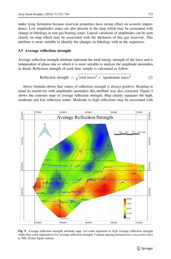
3.5 Average reflection strength

Average reflection strength attribute represent the total energy strength of the trace and is

independent of phase due to which it is more suitable to analyze the amplitude anomalies

in detail. Reflection strength of each time sample is calculated as follow:

Reflection strength ¼ffiffiffiffiffiffiffiffiffiffiffiffiffiffiffiffiffiffiffiffiffiffiffiffiffiffiffiffiffiffiffiffiffiffiffiffiffiffiffiffiffiffiffiffiffiffiffiffiffiffiffiffiffiffiffiffiffiffiffiffiffiffiffiffiffiffiffiffi

ðreal trace)2 þ (quadrature trace)2

q

ð2Þ

Above formula shows that values of reflection strength is always positive. Keeping in

mind its sensitivity with amplitudes anomalies this attribute was also extracted. Figure 9

shows the contours map of average reflection strength. Map clearly separates the high,

moderate and low reflection zones. Moderate to high reflections may be associated with

Fig. 9 Average reflection strength attribute map, red color represent to high average reflection strengthwhile blue color represent to low average reflection strength. Contour spacing between two consecutive linesis 500. (Color figure online)

Acta Geod Geophys (2016) 51:723–744 733

123

major change in lithology, unconformities, stratigraphy as well as hydrocarbon accumu-

lation. The high reflections also represents to gas filled pores or the composite response of

thin beds due to tuning effect (Lynch and Lines 2004). Change in reflection strength in the

map also provide information about the subtle change in lithology, thickness as well as

extent of the reservoir. Map clearly shows that gas producing wells located in the moderate

to strong reflection zones. Overall this map looks like the mirror image of RMS amplitude

attribute map which support the results of above discussed amplitude statistics attributes.

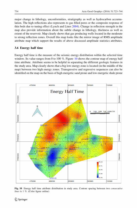
3.6 Energy half time

Energy half time is the measure of the seismic energy distribution within the selected time

window. Its value ranges from 0 to 100 %. Figure 10 shows the contour map of energy half

time attribute. Attribute seems to be helpful in separating the different geologic features in

the study area. Map clearly shows that a big low energy zone is located (in the middle of the

map) between two high energy zones. Transgressive and regressive sequences can also be

identified on the map on the basis of high energetic sand prone and low energetic shale prone

Fig. 10 Energy half time attribute distribution in study area. Contour spacing between two consecutivelines is 1 %. (Color figure online)

734 Acta Geod Geophys (2016) 51:723–744

123

zones. High energy zones indicate that sand facies overly shale facies whereas, low energy

zone indicate that shale facies overlay sand facies. In the map the areas having almost near to

50 % energy half time value indicate that in these areas sand shale facies are homogeneously

distributed. Lateral changes in energy half time can be clearly seen on this map. These lateral

changes in energy may be associated with variation in stratigraphy or amplitude anomalies.

As gas bearing zones are often associated with amplitude anomalies (bright spots). This map

clearly separates the lithological features like shale/sand distribution. Results of this attribute

are more useful than RMS Amplitude, maximum peak amplitude and average reflection

strength maps, as it separates the stratigraphic and amplitudes anomalies more clearly.

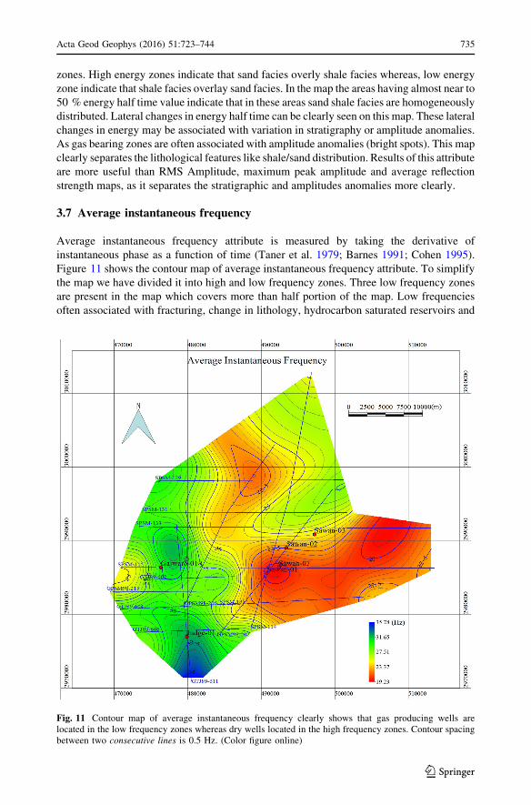
3.7 Average instantaneous frequency

Average instantaneous frequency attribute is measured by taking the derivative of

instantaneous phase as a function of time (Taner et al. 1979; Barnes 1991; Cohen 1995).

Figure 11 shows the contour map of average instantaneous frequency attribute. To simplify

the map we have divided it into high and low frequency zones. Three low frequency zones

are present in the map which covers more than half portion of the map. Low frequencies

often associated with fracturing, change in lithology, hydrocarbon saturated reservoirs and

Fig. 11 Contour map of average instantaneous frequency clearly shows that gas producing wells arelocated in the low frequency zones whereas dry wells located in the high frequency zones. Contour spacingbetween two consecutive lines is 0.5 Hz. (Color figure online)

Acta Geod Geophys (2016) 51:723–744 735

123

particularly with gas saturated sand. Whereas high frequency zones are associated with

non-gas bearing zones and sharp interfaces which may exhibit to thin laminated shale

(Taner et al. 1979). This attribute map clearly indicates that productive wells located in the

very low frequency zone whereas, non-productive wells located in the high frequency

zones. The high frequency zone in the vicinity of Gajwaro-01 well exhibits that this sand

zone is highly interbedded with shale. Figure also shows that Sawan-01 and Sawan-07

wells are located in the lowest frequencies zone. These lowest frequencies correspond to

the strongest gas absorption effects and thickest reservoir zones whereas, high frequency

zones exhibits that reservoirs are thin in those particular places.

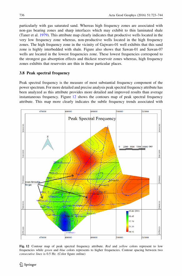
3.8 Peak spectral frequency

Peak spectral frequency is the measure of most substantial frequency component of the

power spectrum. For more detailed and precise analysis peak spectral frequency attribute has

been analyzed as this attribute provides more detailed and improved results than average

instantaneous frequency. Figure 12 shows the contours map of peak spectral frequency

attribute. This map more clearly indicates the subtle frequency trends associated with

Fig. 12 Contour map of peak spectral frequency attribute. Red and yellow colors represent to lowfrequencies while green and blue colors represents to higher frequencies. Contour spacing between twoconsecutive lines is 0.5 Hz. (Color figure online)

736 Acta Geod Geophys (2016) 51:723–744

123

lithological changes and gas bearing sand zones than Fig. 11. Low frequency zones cover the

most part of the map. This map more clearly indicates the lateral variation in frequency, as

wells having thicker gas reservoir are located in the very low frequency zone. One big high

frequency zone is located in lower part (south) of map. High frequencies indicate that sand

reservoir is thin and also include thin laminated shale which, makes these zones not favorable

for gas accumulation. The location of non-productive gas wells (Gajwaro01 and Judge-01) in

the high frequency zone confirms the reliability of the attribute results.

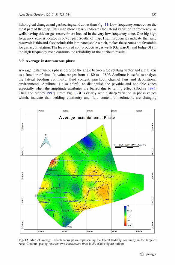
3.9 Average instantaneous phase

Average instantaneous phase describe the angle between the rotating vector and a real axis

as a function of time. Its value ranges from ?180 to -180�. Attribute is useful to analyze

the lateral bedding continuity, fluid content, pinchout, channel fans and depositional

environments. Attribute is also helpful to distinguish the payable and non-able zones

especially when the amplitude attributes are biased due to tuning effect (Bodine 1986;

Chen and Sidney 1997). From Fig. 13 it is clearly seen a sharp variation in phase values

which, indicate that bedding continuity and fluid content of sediments are changing

Fig. 13 Map of average instantaneous phase representing the lateral bedding continuity in the targetedzone. Contour spacing between two consecutive lines is 5�. (Color figure online)

Acta Geod Geophys (2016) 51:723–744 737

123

quickly. So, attributes results reveals that beds are not as continues as other attributes result

indicate. The negative phase values in the map indicate that sands of these zones have good

porosity and good sorting and favorable for gas. Judge-01 well is located in the positive

phase zone which, mean this zone does not have good quality sand so, increase in

amplitude values in this zone are due to tuning effect.

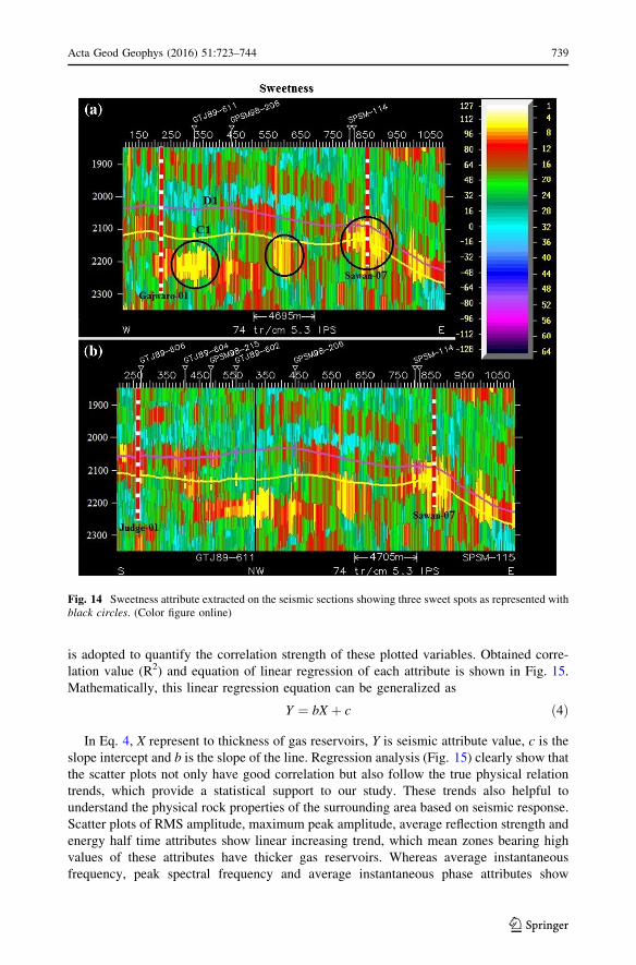
3.10 Sweetness

For more detailed analysis particularly at wells position sweetness attribute was extracted

on the seismic sections. Sweetness is derived by dividing the reflection strength (instan-

taneous amplitude) by the square root of instantaneous frequency (Radovich and Oliveros

1998; Hart 2008). Mathematically it can be expressed as shown in Eq. 3.

Sweetness ¼ InsðAÞffiffiffiffiffiffiffiffiffiffiffiffi

Insðf Þp ð3Þ

where Ins (A) represents instantaneous amplitude (reflection strength) and Ins (f) represents

to instantaneous frequency. Attribute is useful to detect the channels, stratigraphic features

and hydrocarbon reservoirs. Commonly, it is used to distinguish the sand bodies as the

acoustic impedance contrast between sands and shales is relatively higher in the clastic

environments (Hart 2008; Ahmad and Rowell 2012). Figure 14 represent to sweetness

attribute of two seismic sections. Figure 14a represent to seismic line SPSM-115 and

Fig. 14b represent to tie between two seismic lines (SPSM-115 and GTJ 89-611). In the

map the high sweetness zones represent to cleaner and payable sand zones whereas, low

sweetness zones are shale prone or these sands interbedded with shales. In the map three

high sweetness areas can be clearly seen as marked by circles. The position of Sawan-07

well located in this high sweetness zone whereas, Judge-01 and Gajwaro-01 wells are

located in the relatively low sweetness zones in the targeted window. But we can see a high

sweetness zone in the vicinity of Gajwaro-01 well below this targeted window. This good

quality sand zone seems to have potential for producing gas. Munir et al. (2011) also

suggested that this zone (bright spot) have potential for gas if it is evaluated properly. The

3rd zone also seem to have good quality gas sand. Map of this attribute more clearly

separate the productive and non-productive sand zones.

3.11 Statistical analysis

Lateral variations in above discussed seismic attributes maps provide a base for quantifi-

cation analysis. As, seismic attributes also been proven useful for quantification analysis of

reservoir properties. It is common practice to correlate the seismic attribute of interest with

the petrophysical parameter extracted from wireline logs. Commonly regression, geo-

statistics and neural networks methods are used to predict the reservoir properties

(Chambers and Yarus 2002). We used regression method to quantify the relationship

between seismic attributes and petrophysical parameters. In the study area, Sawan-01,

Sawan-02, Sawan-03 and Sawan-07 wells are productive with reservoir thickness 70, 37,

44, 67 m respectively. Analyzed seismic attributes were cross plotted against the thickness

of gas reservoir (Fig. 15) as suggested by White (1991) that cross plotting is helpful for

visual analysis. Visual analysis of these cross plots suggest that linear regression method

can be useful to find the relationship between the plotted variables. (Barnes 2001) also

suggested the same method for amplitude statistics attributes. So, linear regression method

738 Acta Geod Geophys (2016) 51:723–744

123

is adopted to quantify the correlation strength of these plotted variables. Obtained corre-

lation value (R2) and equation of linear regression of each attribute is shown in Fig. 15.

Mathematically, this linear regression equation can be generalized as

Y ¼ bX þ c ð4Þ

In Eq. 4, X represent to thickness of gas reservoirs, Y is seismic attribute value, c is the

slope intercept and b is the slope of the line. Regression analysis (Fig. 15) clearly show that

the scatter plots not only have good correlation but also follow the true physical relation

trends, which provide a statistical support to our study. These trends also helpful to

understand the physical rock properties of the surrounding area based on seismic response.

Scatter plots of RMS amplitude, maximum peak amplitude, average reflection strength and

energy half time attributes show linear increasing trend, which mean zones bearing high

values of these attributes have thicker gas reservoirs. Whereas average instantaneous

frequency, peak spectral frequency and average instantaneous phase attributes show

Fig. 14 Sweetness attribute extracted on the seismic sections showing three sweet spots as represented withblack circles. (Color figure online)

Acta Geod Geophys (2016) 51:723–744 739

123

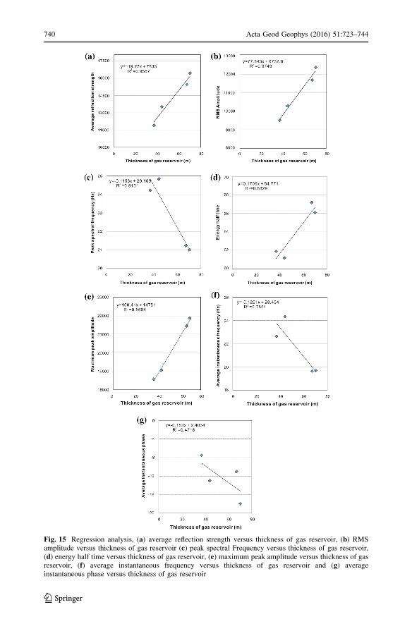
Fig. 15 Regression analysis, (a) average reflection strength versus thickness of gas reservoir, (b) RMSamplitude versus thickness of gas reservoir (c) peak spectral Frequency versus thickness of gas reservoir,(d) energy half time versus thickness of gas reservoir, (e) maximum peak amplitude versus thickness of gasreservoir, (f) average instantaneous frequency versus thickness of gas reservoir and (g) averageinstantaneous phase versus thickness of gas reservoir

740 Acta Geod Geophys (2016) 51:723–744

123

decreasing trends, which mean lower the value of attributes higher the thickness of gas

reservoir. We have found that regression analysis seem to be useful for the quantification of

reservoir thickness in the study area. However, average instantaneous phase does not show

good correlation with the thickness of the gas layer as, this attribute is more suitable to

detect the lateral variation.

4 Discussion

Seismic attributes analysis were performed to interpret the facies units within the targeted

interval in terms of litho-fluid distribution and environments of deposition. The moderate

to high values of amplitude attributes (Figs. 7, 8 and 9) represent to sand bodies and their

direction. The location of producing wells (Sawan-01, 02, 03 and 07) in the moderate to

high amplitude zone (Figs. 7, 8 and 9) indicate that this reservoir interval is composed of

sandstones which, were deposited in the shoreface environments (Sahoo et al. 2014;

Blanke 2013). The distribution of energy content (Fig. 10) indicate that gas producing sand

was deposited in the regressive period whereas, non-productive sand/shale were deposited

in the transgressive period. However, Judge-01 dry well also located in the high amplitude

zone which, creates ambiguity. High values of amplitude attributes in this zone is due to

tuning effect. As, the average instantaneous frequency, peak spectral frequency and phase

attributes clearly indicate that this well is located in the high frequency zone with positive

phase value (Figs. 11, 12 and 13). Very high frequency values in this zone indicate that

reservoir interval is very thin and fall in the seismic resolution limit due to which, the

reflections from the top and bottom of the reservoir interval go to constructive or

destructive interference and causes to produce high amplitude event. These high values of

frequencies also indicate that reservoir zone is highly interbedded with thin laminated shale

layers whereas, lowest values indicates that gas bearing sand reservoir is more thick in this

area. In frequency maps (Figs. 11, 12) contour of 25 Hz clearly draw a boundary between

productive sand and non-productive sand/shale. The payable sands show low to moderate

lateral continuity whereas, non-payable sands/shales show very less continuity (Fig. 13).

To further analyze the lateral as well as vertical variation in the targeted interval, seismic

attribute sweetness was extracted on the seismic sections as shown in Fig. 14. Gas pro-

ducing well (Sawan-07) is located at the shelf edge deltas which hits sweet spot in the

targeted zone (Fig. 14). This sweet spot is bounded by low sweetness zones. This particular

location indicate that shoreface lowstand system tract gas producing sand was deposited on

the distal shaly and silty sediment of the highstand system tract which, was sealed by

transgressive shales and siltstones (Fig. 14). Whereas, Judge-01 and Gajwaro-01 wells are

located in the relatively low sweetness zones and sand of these areas also seems to be in

patches (not well connected). However, two sweet spots can be seen in Fig. 14 bounded by

circles which, seem to be favorable for hydrocarbon potential.

5 Conclusions

Qualitative and quantitative analysis of seismic attributes have been proven helpful in

delineating the gas bearing and non-gas bearing sand zones in the Sawan gas field of

Pakistan. Average instantaneous frequency, peak spectral frequency, average instantaneous

phase and sweetness attributes more clearly distinguish the gas bearing and non-gas

Acta Geod Geophys (2016) 51:723–744 741

123

bearing sand zones, as dry wells are located in the high frequency, positive phase and

relatively in low sweetness zones whereas, gas producing wells are located in the low

frequency, negative phase and high sweetness zones. RMS amplitude, maximum peak

amplitude and average reflection strength attributes clearly mark the high and low values

amplitudes zones, high value of these attributes indicate to sand saturated with gas.

However, these high values of amplitude attributes near the Judge-01 well is due to tuning

effect. Average instantaneous phase and sweetness attributes show that sands in the tar-

geted zone have low to moderate connectivity. Sweetness attribute map show two more

sweet spot indicated by black circles which, seem to be favorable for hydrocarbon

potential. Energy half time attribute proven helpful to identify the transgressive and

regressive sequences. So, we can conclude that the zones which, show high values of

amplitude attributes, energy half time and sweetness, low frequency and negative phase

values are favorable for gas.

Quantitative analysis show that discussed attributes have very good correlation value

(R2[ 0.78) except average instantaneous phase as it is more suitable to analyze the lateral

variations. Amplitude attributes appear to be primary followed by peak spectral frequency,

energy half time and average instantaneous frequency attributes and average instantaneous

phase.

The applied method have some limitations it should be applied in the stable sedimentary

facies zones as the lateral dramatic variation in amplitude causes big change in structure so

method should not be applied in such areas. During the selection of top and bottom

horizons the time window value should be kept in mind because large time window value

will not produce good results.

Acknowledgments The authors are greatly thankful to Directorate General of Petroleum Concession(DGPC), Pakistan for the release of seismic and well data used in this study. We extend our gratefulappreciation to National High-Tech R&D Program of China (2013AA064201) for their financial support tothis study. We also thankful to our lab mates (working at Geo-detection lab, China University of Geo-sciences, Beijing) for their support for the completion of this study.

References

Ahmad MN, Rowell P (2012) Application of spectral decomposition and seismic attributes to understand thestructure and distribution of sand reservoirs within Tertiary rift basins of the Gulf of Thailand. LeadEdge 31:630–634

Ahmad N, Fink P, Sturrock S, Mahmood T, Ibrahim M (2004) Sequence stratigraphy as predictive tool inLower Goru fairway, Lower Middle Indus Platform, Pakistan. PAPG-SPE ATC, pp 85–105

Badly ME (1985) Practical seismic interpretation. IHRDC Publishers, Boston, p 179Barnes AE (1991) Instantaneous frequency and amplitude at the envelope peak of a constant-phase wavelet.

Geophysics 56(7):1058–1060Barnes AE (2001) Seismic attributes in your facies. CSEG Rec 09:41–47Berger A, Gier S, Krois P (2009) Porosity-preserving chlorite cements in shallow –marine volcaniclastic

sandstones: evidence of the sawan gas field Pakistan. AAPG Bull 93(5):595–615Blanke SJ (2013) Saucer sills of the offshore Canterbury Basin. Advantage NZ Petroleum Conference,

AucklandBodine JH (1984) Waveform analysis with seismic attributes. SEG 54th Annual International Meeting,

AtlantaBodine JH (1986) Waveform analysis with seismic attributes. Oil Gas J 84(24):59–63Chambers RL, Yarus JM (2002) Quantitative use of seismic attributes for reservoir characterization. CSEG

Rec 06:15–25Chen Q, Sidney S (1997) Seismic attribute technology for reservoir forecasting and monitoring. Lead Edge

16:445–456

742 Acta Geod Geophys (2016) 51:723–744

123

Chopra S, Marfurt KJ (2005) Attribute review paper—75th Ann of SEG: Draft 3. 15 Mar 2005, p 51Chung HM, Lawton DC (1995) Amplitude responses of thin beds: sinusoidal approximation versus Ricker

approximation. Geophysics 60(3):223–230Cohen L (1995) Time-frequency analysis. Prentice-Hall Signal Processing Series, New YorkDalley RM, Gevers ECA, Stampfli GM, Davies DJ, Gastaldi CN, Ruijtenberg PA, Vermeer GJO (1989) Dip

and azimuth displays for 3-D seismic interpretation. First Break 07(03):86–95Dobrin MB, Savit CH (1988) Introduction to geophysical prospecting. McGraw Hill Book Co., Inc., New

YorkEl-Mowafy H, Marfurt K (2008) Structural interpretation of the middle frio formation using 3D seismic and

well logs: an example from the gulf coast of the United State. Lead Edge 27(7):840–848Fu D, Sullivan EC, Marfurt KJ (2006) Rock-property and seismic attribute analysis of a chert reservoir in the

Devonian Thirty-one Formation, west Texas, USA. Geophysics 71:B151–B158Gholami R, Moradzadeh A, Rasouli V, Hanachi J (2014) Shear wave velocity prediction using seismic

attributes and well log data. Acta Geophys 62(4):818–848. doi:10.2478/s11600-013-0200-7Hart BS (2008) Channel detection in 3-D seismic data using sweetness. AAPG Bull 92:733–742. doi:10.

1306/02050807127Horkowitz KO, Davis DR (1996) Seismic delineation of thin sandstone reservoirs in a shale-rich sequence

using instantaneous frequency and reflection amplitude attributes from 3-D data, Texas Gulf coast.AAPG studies in Geology No. 42 and SEG geophysical Development series No. 5

Iqbal MWA, Shah SMI (1980) A guide to the stratigraphy of Pakistan, Geological Survey of PakistanRecords. Geol Surv Pak Quetta 53:34

Kadri IB (1995) Petroleum geology of Pakistan. Graphic Publishers, Karachi, pp 93–108Khalid P, Ghazi S (2013) Discrimination of fizz water and gas reservoir by AVO analysis: a modified

approach. Acta Geod Geophys 48:347–361. doi:10.1007/s40328-013-0023-7Khalid P, Qayyum F, Yasin Q (2014a) Data driven sequence stratigraphy of the cretaceous depositional

system, Punjab Platform, Pakistan. Surv Geophys 35:1065–1088. doi:10.1007/s10712-014-9289-8Khalid P, Broseta D, Nichita DV, Blanco J (2014b) A modified rock physics model for analysis of seismic

signatures of low gas-saturated rocks. Arab J Geosci 07:3281–3295. doi:10.1007/s12517-013-1024-0Krois P, Mahmood T, Milan G (1998) Miano field, Pakistan a case history of model driven exporation.

Proceedings of the Pakistan Petroleum Convention, Pakistan Association of Petroleum GeologistsIslamabad: pp 111–131

Løseth H, Gading M, Wensaas L (2009) Hydrocarbon leakage interpreted on seismic data. Mar. Petrol Geol26(7):1304–1319. doi:10.1016/j.marpetgeo.2008.09.008

Lynch S, Lines L (2004) Combined attributes displays. 72nd Annual International Meeting, SEG, expandedabstracts, pp 1953–1956

Marfurt KJ, Kirlin RL (2001) Narrow-band spectral analysis and thin-bed tuning. Geophysics 4:1274–1283Marfurt KJ, Kirlin RL, Farmer SL, Bahorich MS (1998) 3-D seismic attributes using a semblance-based

coherency algorithm. Geophysics 63:1150–1165McPhee CA, Enzendorfer CK (2004) Sand management solutions for high-rate gas wells, sawan field. SPE,

Sindh (86535)Munir K, Iqbal MA, Farid A, Shabih SM (2011) Mapping the productive sands of Lower Goru Formation by

using seismic stratigraphy and rock physical studies in Sawan area, southern Pakistan: a case study.J Petrol Explor Prod Technol 1:33–42. doi:10.1007/s13202-011-0003-9

Radovich BJ, Oliveros RB (1998) 3-D sequence interpretation of seismic instantaneous attributes from theGorgon field. Lead Edge 17:1286–1293. doi:10.1190/1.1438125

Raef AE, Mattern F, Philip C, Totten MW (2015) 3D seismic attributes and well-log facies analysis forprospect identification and evaluation: interpreted palaeoshoreline implications, Weirman Field, KS,USA. J Petrol Sci Eng. doi:10.1016/j.petrol.2015.04.028

Rana S, Burley S, Chowdhury S (2006) The application of hierarchical seismic attribute combination to highprecision infill well planning in the South Tapti Field, Offshore Western India. GEOHORIZONS. J SocPet Geophy 11:32–37

Robertson JD, Nogami HH (1984) Complex seismic trace analysis of thin beds. Geophysics 49(4):344–352.doi:10.1190/1.1441670

Sahoo TR, Browne GH, Hill MG (2014) Seismic attribute analysis and depositional elements in the Can-terbury Basin. GNS Science, Lower Hutt

Sonneland L, Barkved O, Olsen M, Snyder G (1989) Application of seismic wave-field attributes inreservoir characterization: 59th Annual International Meeting, Society of Exploration Geophysicists,p 813

Taner MT (2001) Seismic attributes, CSEG Recorder, pp 48–56, September IssueTaner MT, Koehler F, Sheriff RE (1979) Complex seismic trace analysis. Geophysics 44(6):1041–1063

Acta Geod Geophys (2016) 51:723–744 743

123

Taner MT, Schuelke JS, Doherty RO, Baysal E (1994) Seismic attributes revisited, SEG technical program,expanded abstracts. pp 1104–1106, doi: 10.1190/1.1822709

Wandrey CJ, Law BE, Shah HA (2004) Sembar goru/Ghazij composite total petroleum system Indus andsulaiman-kirthar geologic provinces Pakistan and India. US Geological Survey, USA; Geol Surv Bull2208-C

Wang Z, Yin YC, Fan T, Lei X (2012) Seismic geomorphology of a channel reservoir in lower Min-ghuazhen Formation, Laizhouwan sub-basin, China. Geophysics 77(4):187–195. doi:10.1190/geo2011-0209.1

White RE (1991) Properties of instantaneous seismic attributes. Lead Edge 10(7):26–32Widess MB (1973) How thin is a thin bed. Geophysics 38:1176–1180Ye TR, Su JY, Liu XY (2008) Application of seismic frequency division interpretation technology in

predicting continental sandstone reservoir in the west of Sichuan province. Geophys Prospect Petrol47(1):72–76

Yushuang Hu, Zhu Simiao (2013) Predict channel sand body distribution characteristics of south eighthdistrict based on RMS amplitude attributes & frequency division. Adv Mater Res 734:404–407

744 Acta Geod Geophys (2016) 51:723–744

123