This paper presents preliminary findings and is being distributed to economists

and other interested readers solely to stimulate discussion and elicit comments.

The views expressed in this paper are those of the authors and do not necessarily

reflect the position of the Federal Reserve Bank of New York or the Federal

Reserve System. Any errors or omissions are the responsibility of the authors.

Federal Reserve Bank of New York

Staff Reports

An Anatomy of U.S. Personal Bankruptcy

under Chapter 13

Hülya Eraslan

Gizem Koşar

Wenli Li

Pierre-Daniel Sarte

Staff Report No. 764

January 2016

An Anatomy of U.S. Personal Bankruptcy under Chapter 13

Hülya Eraslan, Gizem Koşar, Wenli Li, and Pierre-Daniel Sarte

Federal Reserve Bank of New York Staff Reports, no. 764

January 2016

JEL classification: C61, D12, K35

Abstract

We build a structural model of Chapter 13 bankruptcy that captures salient features of personal

bankruptcy under Chapter 13. We estimate our model using a novel data set that we construct

from bankruptcy court dockets recorded in Delaware in 2001 and 2002. Our estimation results

highlight the importance of debtor’s choice of repayment plan length for Chapter 13 outcomes

under the restrictions imposed by the bankruptcy law. We use the estimated model to conduct

policy experiments to evaluate the impact of more stringent provisions of Chapter 13 that impose

additional restrictions on the length of repayment plans. We find that these provisions would not

materially affect creditor recovery rates and would not necessarily make discharge more likely for

debtors with income above the state median.

Key words: Chapter 13 bankruptcy, discharge, recovery rate

_________________

Eraslan: Rice University (e-mail: eraslan@rice.edu). Koşar: Federal Reserve Bank of New York

(e-mail: gizem.kosar@ny.frb.org). Li: Federal Reserve Bank of Philadelphia

(e-mail: wenli.li@phil.frb.org). Sarte: Federal Reserve Bank of Richmond

(e-mail: pierre.sarte@rich.frb.org). The authors are grateful to Philip Bond, Bob Hunt, Steven

Stern, Kenneth Wolpin, Holger Sieg, and two anonymous referees for helpful comments and

suggestions. They also thank seminar participants at the University of Pennsylvania, the Federal

Reserve Bank of Philadelphia, the Federal Deposit Insurance Corporation (FDIC), the 2007

Society of Economic Dynamics Summer Meetings, Florida International University, Southern

Methodist University, the University of Oxford, and the University of Virginia. Ishani Tewari and

Sarah Carroll provided excellent research assistance. The authors acknowledge financial support

from the FDIC Center for Financial Research, the Wharton Financial Institutions Center, and the

Rodney L. White Center for Financial Research. Finally, they are indebted to Michael Joseph, the

Chapter 13 Trustee for the District of Delaware, for numerous conversations and e-mail

exchanges that have enhanced their understanding of bankruptcy law and its practice. The views

expressed in this paper are those of the authors and do not necessarily reflect the position of the

Federal Reserve Bank of Philadelphia, the Federal Reserve Bank of Richmond, the Federal

Reserve Bank of New York, or the Federal Reserve System.

In short, the bankruptcy system operates behind a veil of darkness created by the lack of reliabledata about its operations. The lack of information about “what is going on” in the bankruptcy systemleads to a distrust of its results – a belief by some that creditors, debtors, and professionals withinthe system are all somehow taking advantage of one another and the public at large, and that thesystem suffers from widespread fraud, abuse, and inefficiency.

1997 National Bankruptcy Commission

1 Introduction

On April 20, 2005, the Bankruptcy Abuse Prevention and Consumer Protection Act (BAPCPA)was signed into law and ended a comprehensive legislative effort that began under the Clintonadministration. The most significant (and controversial) change introduced by the new personalbankruptcy law was to impose a “means test” on debtors contemplating a bankruptcy filing. Theaim was to ensure that debtors with sufficient income would file under Chapter 13 and complete arepayment plan out of future income. The key presumption underlying this provision was that alarge number of households did not repay as much as their income allowed. In particular, it wasthought that Chapter 13 would perform better, both as a collection device for creditors and as ameans to provide debtors with a financial fresh start, if stricter rules were imposed on repaymentplans.1

The objective of our paper is to take a first step at evaluating the impact of these stricterrules. Specifically, we aim to assess the effect of section 1325, paragraph 4, which was added tothe U.S. Bankruptcy Code under BAPCPA and imposes additional restrictions on the length ofrepayment plans for debtors with income above the state median. In order to do so, we build andestimate a structural model of Chapter 13 bankruptcy using a novel data set we construct. Fora side contribution, we provide empirical evidence regarding the outcomes under Chapter 13 andits performance both as a collection device for creditors and as a means to provide debtors with afinancial fresh start.

Our model captures the salient features of personal bankruptcy under Chapter 13. In our model,a debtor first makes decisions regarding whether or not to file under Chapter 13 and, if so, whatrepayment plan to propose. Since the law requires that all of a debtor’s excess income be appliedto his repayment plan, the debtor’s choice of repayment plan boils down to its length2. In choosingwhat plan to propose, the debtor recognizes that its duration has a bearing on the confirmationoutcome that is determined by the recommendations of a bankruptcy trustee appointed to overseethe bankruptcy process. Under the bankruptcy law, in deciding whether to confirm a plan ornot, the trustee must form an opinion as to the fairness and feasibility of the plan. The fairnesscondition is satisfied as long as the debtor contributes all excess income into the plan payments.The feasibility condition requires that the debtor’s excess income is sufficient to pay the unsecuredcreditors over a three- to five-year period an amount no less than they can recover under liquidationof the debtor’s assets. To capture the idea that the trustee has some leeway in the interpretationof the bankruptcy law, in our model, whether the trustee views a given plan as fair and feasible ornot is random from the perspective of the debtor. Specifically, whether the trustee views a plan asfair and feasible depends on the debtor’s characteristics and the plan length.

Even if a plan is initially confirmed, it may nonetheless become unfair or infeasible due tofluctuations in the debtor’s financial condition. We model this possibility by introducing shocks to

1See, for example, https://www.tinyurl.com/bapcpa2005.2Excess income is income minus necessary expenses including housing payments either in the form of rent or in the

form of mortgages. Note that the mortgage debt that is not yet due is paid outside the Chapter 13 repayment plan.

1

income or expenses of the debtor at a random date. Following the shocks, the trustee reevaluatesthe feasibility of the plan under the new debtor characteristics. If the case is not dismissed, thedebtor decides whether to continue or voluntarily default on his plan.

Overall, our model highlights a basic trade-off debtors face in proposing long repayment plansversus short ones. Long repayment plans are costly in that they impose restraints on debtors forlonger periods, but these plans may also be more likely to be confirmed by the court and, ultimately,to result in a financial fresh start. In addition, our model highlights the importance of shocks toexcess income during the bankruptcy process. In particular, even though a plan may be fair andfeasible at the time a debtor files for Chapter 13 bankruptcy, it may cease to be so later on beforethe repayment plan is complete.

We estimate our model using newly collected data contained in court files on all Chapter 13personal bankruptcies recorded by the United States Bankruptcy Court for the District of Delawarebetween August 2001 and August 2002. From the court documents, we extract information con-cerning the filers’ financial and demographic information at the time of filing and the final outcomeof their cases. Specifically, we collect data on the outcomes predicted by our model: the choice ofplan length, whether the plan is confirmed or not, whether the case is successfully completed or not,and the recovery rate of the creditors.3 In addition to these endogenous outcomes, in our model thedecision to file for Chapter 13 in the first place is also endogenous. Although all the debtors in oursample have chosen to file for Chapter 13, we identify the parameters associated with this decisionthrough the variation in the decision to continue or voluntarily default on the plan following theshocks to financial conditions.

We estimate our model using the maximum likelihood approach. Our estimates confirm thatthe debtor’s choice of plan length indeed affects the trustee’s opinions on the fairness and feasibilityof the plan. In particular, after controlling for exogenous debtor characteristics, we find that longerplans are more likely to be confirmed in the first place and less likely to be dismissed after theoriginal plan becomes infeasible. However, whether a debtor’s income is above the state medianlevel does not play a significant role in the confirmation of the plan.4 As such, the means testestablished under BAPCPA appears inconsequential. In addition, we find that the timing of thechanges in debtors’ conditions during bankruptcy play a significant role in governing Chapter 13outcomes, including the ability of debtors to obtain a financial fresh start. In particular, whennegative shocks to income are experienced early in the program, the probability of dismissal risessignificantly.

We next conduct policy experiments to assess the effect of section 1325, paragraph 4, that wasadded to the U.S. Bankruptcy Code under BAPCPA. This policy imposes additional restrictions onthe length of payment plans for debtors with income above the state median. Our results predictthat this new policy would not materially affect creditor recovery rates and would not necessarilymake discharge more likely for debtors with income above the state median. This finding is robustto alternative policy experiments that require bankruptcy plans to meet stricter standards in otherways, such as proposing a higher recovery rate. In fact, in these alternative experiments, someChapter 13 filers no longer choose to file, with the result that recovery rates and discharge rateseven decline. It appears, therefore, that a stricter bankruptcy code can make it more difficult fordebtors to obtain a fresh start but without necessarily helping to raise creditor recovery rates.

It is well understood that personal bankruptcy laws affect credit markets, and therefore thesupply and demand for credit (Gropp, Scholz, and White (1997) and Lin and White (2001)), the

3Throughout the paper, by recovery rate of the creditors, we mean their recovery within Chapter 13. It is possiblethat the creditors collect payments outside Chapter 13 as well. We return to this possibility in Section 7.3.

4Whether income is above the state median appears immaterial for the confirmation of the plan; however, incomeplays an important role through the determination of excess income and therefore the required plan payments.

2

ability of households to insure against labor income risk (Athreya et al., 2012), their consumptionbehavior (Filer and Fisher (2005) and Grant (2004)), labor supply (Han and Li, 2007), mobility(Elul and Subramanian, 2002), entrepreneurial activity (Meh and Terajima (2008) and Mankartand Rodano (2015)).

Given that the effect of the personal bankruptcy laws on these economic outcomes is throughthe decision to file for bankruptcy in the first place, it is important to understand the determinantsof households’ bankruptcy and default decisions. In early work Domowitz and Sartain (1999) usea nested logit model to estimate consumers’ decisions to file for bankruptcy and their choice ofbankruptcy chapter but they take a reduced form approach for values of each of these decisions.Gross and Souleles (2002) estimate a dynamic probit model of default using individuals’ creditcard account data and conclude that the increase in the bankruptcy filing rates between 1995and 1997 cannot be explained by risk factors and economic conditions alone. In their analysis,they do not distinguish between different default options. Using data from the Panel Study ofIncome Dynamics Fay, Hurst, and White (2002) test whether households are more likely to filefor bankruptcy if the financial benefits from filing for bankruptcy is higher. They compute thefinancial benefits from filing for bankruptcy using the Chapter 7 bankruptcy alternative alone. Ourpaper contributes to the literature on household bankruptcy default decisions5 and complementsthese papers by endogenizing the value of the Chapter 13 bankruptcy alternative using a structuralmodel that explicitly takes into account the choices made by the debtors within Chapter 13 and theuncertainties they face.6 Moreover, by considering the particular channels through which observableand unobservable debtor characteristics affect bankruptcy outcomes, we are able to provide anassessment on how changes in bankruptcy law might alter the outcomes in Chapter 13, and thereforethe value of filing for Chapter 13.

Like us, Sullivan et al. (2003), Norberg and Velkey (2006) and White and Zhu (2010) constructdata on Chapter 13 bankruptcy filers using U.S. bankruptcy court files. The focus of the first twopapers are entirely descriptive, while White and Zhu (2010) focuses on the debtors’ decisions todefault on their mortgages and file for bankruptcy. By contrast, our main focus is on the decisionsof the debtors after filing for Chapter 13 bankruptcy.

Finally, our paper also informs a literature in macroeconomics that has provided tractable modelsrelating documented empirical facts on consumer bankruptcy to aggregate considerations. A numberof these studies have used calibration and simulation exercises to explain observed aggregate U.S.consumer bankruptcy filing rates and have evaluated the effects of information, financial innovation,and changes in bankruptcy laws on these rates and other economic aggregates. Some papers in thisliterature either explicitly state that they model bankruptcy in a way to capture Chapter 7, or modelbankruptcy as loss of assets as opposed to loss of income thus resembling Chapter 7 as opposed toChapter 13 (e.g. Athreya (2002); Chatterjee et al. (2007); Livshits et al. (2007, 2011), Chatterjeeand Gordon (2012), Gordon (2015)). Others are agnostic about what happens after bankruptcy butinclude an implicit or explicit cost as a function of income (e.g. Drozd and Nosal (2008) and Sanchez(2010)). In that sense, these papers can be interpreted as capturing some elements of Chapter 13.The only paper we are aware of which explicitly distinguishes between Chapter 7 and Chapter 13is Li and Sarte (2006) who model Chapter 7 as a loss of assets and Chapter 13 as a loss of incomeresulting in full discharge of debt. As we show, only 44% of the debtors who file for Chapter 13 areable to obtain discharge. Overall, the main difference between the macro literature on bankruptcyand our current paper is that we make use of micro data and we do not take Chapter 13 outcomes

5There are also related studies looking at bankruptcy filings at the state level. See, for example, Dick and Lehnert(2010), Cornwell and Xu (2014) and Gross, Notowidigdo, and Wang (2014).

6See Eckstein and Wolpin (1989); Rust (1996); Aguirregabiria and Mira (2010), and Keane et al. (2011) for surveysof structural dynamic choice models.

3

as given.The remainder of this paper is organized as follows. Section 2 presents institutional details

associated with U.S. personal bankruptcy law as well as a summary of creditors’ options outsidebankruptcy. Section 3 provides a description of the data. Section 4 presents a structural modelof Chapter 13 bankruptcy. Section 5 presents econometric specification. Section 6 presents ourestimation results. Section 7 assesses the effects of policy experiments directly related to BAPCPAas well as hypothetical ones. Section 8 offers some concluding remarks.

2 Legal Background

This section first briefly reviews creditors’ legal remedies outside bankruptcy. It then addressesthe main features of U.S. personal bankruptcy law focusing in detail on Chapter 13 court procedures.

2.1 Creditors’ Legal Remedies Outside of Bankruptcy

When a debtor defaults on his debt obligations without explicitly filing for bankruptcy, securedcreditors, such as mortgage lenders or car loan lenders, seize property to recover what they are owed.Unsecured creditors, such as credit card issuers, often start with making calls and writing letterssoliciting payments. They then typically sell their debts to collecting agencies. Unsecured creditorsalso have the option to sue the debtor and obtain a court judgment against him. They collect onthe judgment by having the court order that the debtor’s employer take a portion of his paycheckand remit that money to the sheriff, who then forwards the payment appropriately. This processis known as “wage garnishment.” Unsecured creditors can also potentially seize a debtor’s bankaccount and/or foreclose on his home. State laws typically restrict the amount and type of assetsthat can be seized to different degrees. Therefore, the process of seizing an account or foreclosingon a property can be costly and, in practice, unsecured creditors rarely do so.

2.2 Main Features of U.S. Personal Bankruptcy Law Prior to BAPCPA

U.S. personal bankruptcy law features two distinct procedures: Chapter 7 and Chapter 13.Prior to BAPCPA, debtors had the right to choose between the two chapters.7 Chapter 7 is oftenreferred to as “liquidation.”Under Chapter 7, the debtor surrenders all assets above an exemptionlevel that varies across states. In exchange, he obtains the discharge of most of his unsecured debtsuch as credit card debt, medical bills, personal loans, utility bills, etc.8 A debtor cannot file againfor Chapter 7 during the six years that follow the last filing. In contrast, Chapter 13 is formallyknown as “adjustment of debts of consumers with regular income.”Under Chapter 13, a portion ofa debtor’s future earnings are used to meet part of his debt obligations. The repayment plan canlast for a period of up to five years. While the debtor’s assets are unaffected under Chapter 13, atthe end of the payment plan, any remaining debt is discharged. A debtor is prevented from filingagain under Chapter 13 for a period of 180 days following his last filing.

2.3 Bankruptcy Procedure under Chapter 13

A Chapter 13 case begins when a debtor files a petition with the bankruptcy court. Thispetition gives a description of, among other information, the debtor’s assets, debts, income, and

7Given the time span covered by our data set and the objectives of this paper, the basic features of personalbankruptcy law we provide below predate the passage of the 2005 Bankruptcy Reform Act.

8Discharge prevents the creditors who are owed the discharged debts from taking any action against the debtor,including any communication with the debtor regarding unpaid debts.

4

expenditures. In the petition, the debtor also proposes a repayment plan that devotes all of his excessincome to the payment of unmet claims. Bankruptcy law defines excess income as any income netof necessary living expenses including housing expenses, which is in the form of mortgage paymentsfor most of the debtors. In order to be confirmed by the court, the proposed plan must provide torepay the debt over a three- to five-year period. It must also be filed in good faith.9 In particular,the debtor must propose to pay at least as much as the value of the assets creditors would haveotherwise received under Chapter 7. Finally, the plan must cure any default on secured debt at thetime of filing before providing for payments to unsecured creditors. Because the law requires debtorsto devote all of their disposable income to the payment plan, the key element of the repayment planis the proposed plan length.

Upon the filing of a petition, a trustee is appointed by the bankruptcy court. The trusteeis responsible for evaluating and recommending whether or not to confirm a proposed plan. Healso works as a disbursing agent during the implementation of the plan, collecting payments fromdebtors and distributing them to creditors. Within a month of the petition filing, the trusteeschedules a section 341 meeting. At this meeting, creditors are given an opportunity to ask anyquestions regarding the debtor’s financial situation that may affect the plan. Ultimately, the trusteerecommends to the court that a proposed plan either be confirmed, along with the implied repaymentschedule, or be dismissed.

If the plan is dismissed, the case ends. Creditors can resume legal remedies outside bankruptcy,as described above, to pursue the repayment of their loans. If a repayment plan is confirmed, thedebtor starts making payments as specified in that plan.10 Once plan payments are completed, anyremaining debt is discharged. It is possible for a plan that is initially confirmed to be subsequentlyaltered. In particular, the debtor is free to prepay his debts in the event that his assets appreciateor he receives additional income from an unexpected source, such as an inheritance. The debtorcan also potentially convert the case to a Chapter 7 filing, even after confirmation of the Chapter13 plan, or voluntarily default on the confirmed plan and have the case dismissed. When a debtorbenefits from a substantial increase in income after confirmation of a repayment plan, the lawrequires the debtor to increase his payments by the amount of additional income received (unlessexpenses for basic maintenance have also changed). Ultimately, the final plan that is carried outcan look very different from the proposed and confirmed plan.

3 The Data

3.1 Data Collection

The data collected in this paper are obtained using an electronic public access service to caseand docket information from Federal Bankruptcy courts and the U.S. Party/Case Index. Thisservice is known as Public Access to Court Electronic Records (PACER) and offers bankruptcycourt information including i) a listing of all parties and participants including judges, attorneys,and trustees, ii) a chronology of the dates of case events entered in the case record, iii) a claimsregistry, and iv) the types of documents filed for specific cases and imaged copies of these documents.

The docket sheet together with the court files it contains allow us to extract information con-cerning important dates that mark the Chapter 13 bankruptcy procedure, including the filing date,

9Trustees typically ask Chapter 13 filers to start submitting periodic payments according to the plan as soon asthe plan is filed. Payments are distributed to creditors only if the plan is confirmed and are otherwise refunded.This practice, together with other court rules, discourages debtors from staying in Chapter 13 bankruptcy without aconfirmed plan for too long.

10In Delaware, the trustee receives 6% of total payments made under a confirmed plan.

5

the confirmation date, and the dismissal or discharge date, as well as filers’ financial and incomeinformation at the time of filing and the final outcome of the case. The court files include debtor pe-titions, attorney disclosure forms, statements of financial affairs, Chapter 13 plans, and the trusteereport. The debtor petitions contain different schedules, labeled A through J, that set forth thefinancial situation of the debtor, including real property that is owned, other personal assets inthe form of furniture, cash, or insurance, liabilities such as secured debt and unsecured prioritydebt (taxes), and maintenance expenses for food, clothes, and transportation, among other basicexpenses.

The court files are mostly PDF images from which information cannot be directly extracted usingsoftware. We manually collected all of our data by downloading these images and coding them intoa database. The data were entered twice and the corresponding entries were cross-checked. Thedata were also checked against different sources where the same information was reported. Forinstance, the summary of schedules provides headline numbers on filers’ assets, debts, income, andexpenditures, while petition schedules A through J provide the same information in greater detail.

There were 1, 085 Chapter 13 bankruptcy cases filed in Delaware over our sample period (August2001 to August 2002). Of the 1, 085 cases, we deleted from our sample 134 cases that have incompleteinformation resulting from either court recording or filing errors, and that were therefore triviallydismissed. In addition, 130 cases were omitted from the data due to inconsistent information filedby the debtors. Our final sample contains 821 cases, of which 364 (or 44%) resulted in a dischargeupon successful completion of the repayment plans while 457 cases were dismissed under Chapter13. Of the dismissed cases, 52 were later converted to Chapter 7 filings. Table 1 summarizes thisinformation.

3.2 Data Description

3.2.1 Selected Characteristics of Chapter 13 Debtors

Most of the variables we use in our analysis are directly available from the court files. Others areconstructed on the basis of these original variables.11 For comparison, demographics, employmentstatus, and income information are obtained for the State of Delaware from the 2000 Census and theMortgage Bankers Association. We also report data on expenditures from the northeast region ofthe 2001 Consumer Expenditure Survey. Balance sheet information at the national level is obtainedfrom the 2001 Survey of Consumer Finances.

The debtors in our sample are somewhat less likely to be unemployed than the average Delawareresident, with approximately 4% of the filers being unemployed compared to 5% in Delaware. Thisis not surprising since Chapter 13 bankruptcy is designed for curing the debts of individuals withregular income. What is more surprising is that about 5% of the filers are self-employed. Averagemonthly household income for the debtors in our sample is $2, 938, which falls short of Delaware’saverage adjusted gross income by about 30%. Filers for whom we have income data for both thecurrent and previous year experience a nearly 20% average decline in income prior to filing.

The court files also provide information regarding debtors’ monthly expenses that define basicmaintenance under Chapter 13. Debtors in our sample spend on average $1,164 on housing expenses(mortgage or rent). While housing expenses are shielded by law, a provision prohibits debtors fromboosting these expenses prior to filing. In our sample, housing expenses, including expenses for

11One such variable is excess income. We don’t observe actual income in our data. However, we have informationon the proposed payment and the proposed pay length. Since in Chapter 13 bankruptcy the debtors need to put allof their disposable income after paying out the necessary expenditures into bankruptcy, we construct excess incomeusing information from proposed payments and proposed paylengths.

6

home maintenance, account on average for 40% of total monthly expenses.12 Debtors in Chapter 13spend about $442 a month on average for food and clothing, which is considerably less than the $600monthly average reported for the northeast region of the Consumer Expenditure Survey. Food andclothing represent 19% of debtors’ monthly expenses in our sample. The remaining categories thatdefine maintenance expenses include alimony payments,13 insurance premia, medical expenditures,transportation expenses, and discretionary expenses. Discretionary expenses include recreation andentertainment. These expenses are arguably the least related to basic necessities and the mostsubject to interpretation by the trustee. In our sample, however, discretionary expenses accountfor approximately 2.5% of total monthly expenses on average.

We refer to a debtor as a repeat filer if he has filed for either Chapter 7 or Chapter 13 bankruptcyat least once prior to the current filing, since 1980. In our sample, about 24% of the debtors arerepeat filers and thus have already been exposed to the experience of bankruptcy.

As expected, the most striking aspect of Chapter 13 filers relates to their level of indebtedness.Specifically, their median total debt, including mortgages, car loans, and credit card debt, is about$121,852, around six times the national median, while their median total assets are $104,000, lessthan half of the corresponding national median. Their median unsecured debt is $14,737, comparedto a national median of zero. Median arrears14 amount to $12,517. Together, total debt in defaultfor the median filer - arrears as well as unsecured debt - amounts to approximately to the debtor’sannual gross income. Specifically, the debtor with the median income earns $31,284 and the debtorwith the median total debt in default owes $30,834 in past-due debt. By contrast, the debtor withthe median total debt, including mortgages, car loans, and credit card debt, owes about $121,852.The large difference is due to the fact that some of the debt is not in default.

Table 2 provides summary statistics for the debtor characteristics we use in our analysis. As canbe seen from this table, monthly rent or mortgage payments average a little under $850 a month,which amounts to about 31% of monthly income. For about 8.5% of filers, medical debt constitutesover 10% of their total debt in default.15 About a quarter of filers have above-state-median-incomeat the time of filing. Moreover, on average, the debtors in our sample have been in their currentjob for about five months. A little over 1% of the filers did not hire an attorney. Those who didhired experienced attorneys in the sense that their attorneys handled, on average, 94 cases in oursample. Finally, the majority of the filers proposed long repayment plans (over four years), withthe proposed recovery rates over 65%.

To sum up, Chapter 13 filers in our sample tend to earn noticeably less than average and are veryheavily indebted. These observations are broadly consistent with previous findings in the literature(see, for example, Domowitz and Sartain (1999); Nelson (1999), and Fay et al. (2002)).

3.2.2 Outcomes under Chapter 13

Two of the key outcomes of the personal bankruptcy process are creditors’ recovery rate anddebtors’ ability to obtain a discharge. These outcomes depend crucially on the length of plans that

12About 87% of the debtors in our sample own their homes, which exceeds the 70% state homeownership rate. Thatsaid, over one-fifth of homeowners who file for bankruptcy have pending foreclosure lawsuits, much higher than thestate average foreclosure rate of 0.35%.

13Compared to their peers, Chapter 13 filers in our sample are less likely to be married, with 46% of the samplebeing recorded as married versus 54% for the state of Delaware. Approximately 6% of the filers listed alimony as partof either their monthly income or monthly expenses, thus suggesting a recent divorce.

14Arrears are missed payments that are past due on a (secured) loan. This is particularly relevant for mortgagedebt in the case of consumer bankruptcy. For secured debt, the part of the debt that is in default is only the arrears.

15We calculate medical debts by flagging keywords such as “health,”“medical,”or “Labcorp,”that are listed foreither the debt type or the associated creditor.

7

are chosen by debtors and whether these plans are confirmed16 by the trustee. Hence, this paperfocuses on these four quantifiable aspects of Chapter 13.

Figures 1 and 2 illustrate noteworthy aspects of proposed Chapter 13 plans in our sample. First,proposed plan lengths in Figure 1 are nearly bimodal, with the majority of filers proposing eitherthree-year or five-year plans. In what follows, we will refer to plans shorter than four years asthree-year plans and the plans longer than four years as five-year plans.

The fact that a large fraction (84%) of the debtors propose five-year plans is not surprising giventhat it often takes at least three years for filers to repay arrears in full.

Second, there exists considerable variation in proposed creditor recovery rates. As shown inFigure 2a, the majority of filers propose to repay at least half of their total debt in default. The meanand median proposed recovery rates are close to 66 cents and 60 cents on the dollar, respectively.Around 20% of filers propose to pay their creditors back in full.

Third, as illustrated in Figure 2b, these recovery rates are strikingly lower than those implied bythe proposed plans. An important reason for the discrepancy is that many debtors in bankruptcyend up not carrying out their plans in full, either because they are dismissed by the trustee at a laterstage or because they voluntarily exit Chapter 13 before completing their plans. Accordingly, thedistribution of actual recovery rates looks very different, depending on whether debtors completedChapter 13 and were successfully discharged or not. This is shown in Figure 3a. Furthermore,Figure 3b illustrates that the proposed plan length also matters somewhat for the distribution ofrecovery rates. Interestingly, although their average recovery rates are similar, debtors that proposefive-year plans are associated with a lower median recovery rate than those that propose three-yearplans. Specifically, the actual median recovery rates are 15% for the debtors with five-year plansversus 19% for the debtors with three-year plans. One possible reason is that debtors who seek tosmooth their payments over longer periods could be the ones in greater financial distress.

The average recovery rate for the creditors is 29%, with a median recovery rate of 14%. Themean and median recovery rates conditional on the debtor being discharged are 59% and 55%,respectively.17 This recovery rate is the weighted average of the recovery rates of the unsecuredand secured creditors. The mean recovery rate on unsecured debt is 17% while the median is 0%.Conditional on discharge, the mean and median recovery rates on unsecured debt are 38% and25%, respectively. By contrast, the mean recovery rate on secured debt is 49% while the medianis 39%. By law, the recovery rate on secured debt conditional on discharge must be 100%. Theunconditional recovery rate on secured claims is, however, lower than 100% for two reasons. First,when the debtor does not obtain a discharge in Chapter 13, he does not necessarily pay his securedcreditors in full. Second, for secured debt other than mortgages (for example, car loans), it ispossible that the value of the claim is reduced during the bankruptcy proceedings through cram-down. Although we do not have the data on cram-down, we do not expect the recovery rates wereport to be too different from the actual recovery rates since most of the secured debt is mortgagedebt, which cannot be crammed down.

The descriptive statistics for the variables we just discussed as well as the remaining outcomesare summarized in Table 3. As can be seen, close to 20% of the cases in our sample are dismissedwithout ever obtaining the confirmation of a plan, and only 55% of the confirmed plans are carriedout to completion. In summary, creditor recovery rates are considerably lower than those that arefirst proposed. In addition, more than half of the debtors fail to obtain the financial fresh startpotentially afforded by the bankruptcy law. A natural question is this: what debtor characteristics,

16Cases that are not confirmed are either converted to Chapter 7 or dismissed. Given the small number of Chapter7 conversions in our sample, we do not formally distinguish between dismissal and chapter conversion in our analysis,even though a case that is converted to Chapter 7 may eventually be discharged under that chapter.

17Chapter 13 recovery rates are necessarily zero for cases that are dismissed without confirmation.

8

or other aspects of Chapter 13, are associated with these outcomes? To answer this question, thenext section builds a structural model of Chapter 13 bankruptcy.

4 The Model

In this section, we model the behavior of debtors while they are in Chapter 13 bankruptcy,taking as given trustees’ decision rules. We do not explicitly model the creditors’ problem sincethey don’t actively participate in the bankruptcy process.

Our analysis begins with a debtor’s decision to file for bankruptcy under Chapter 13. We letF ∈ {0, 1} denote the debtor’s decision to file for Chapter 13 bankruptcy, where F = 1 if andonly if the debtor files for Chapter 13. In order to be able to discharge his debts, the debtor mustpropose a repayment plan, have it confirmed by the court, and carry it out in full. The payoff ofthe debtor depends on the payments P he makes in Chapter 13 and whether or not he obtains adischarge. We let D ∈ {0, 1} denote the discharge outcome, where D = 1 if and only if a dischargein Chapter 13 is obtained. The payoff from discharge is normalized to zero, and the payoff fromoutside options (as well as exiting Chapter 13 without a discharge) is given by V (Z), where Zdenotes the predetermined debtor characteristics at the time of filing for bankruptcy.18 We assumethat the payoff of the debtor is additively separable over payments and the discharge outcome andthat it is given by u(P,D) = −P + (1−D)V (Z).

Since the law requires all of the debtor’s excess income to be applied to the repayment plan,he has little say over per-period plan payments, and these are treated as exogenous. As discussedin the previous section, discretionary expenses account for a negligible fraction of the monthlyexpenses. As such, we assume the monthly payment amount is exogenously given by the excessincome, denoted by X, and the debtor’s choice regarding the plan consists solely of its length. Weassume the debtor can propose either a three-year (short-term) plan or a five-year (long-term) plansand we denote the plan length by L.19

Once a plan is proposed, a trustee must decide whether or not to confirm the proposed plan.We assume that the trustee is nonstrategic and that his decision rule is exogenous, which the debtortakes as given. In addition, we assume that the decision rule is stochastic. This captures the ideathat the interpretation of the bankruptcy law is not entirely unambiguous, and the trustee has someleeway in the interpretation of its provisions. How the trustee interprets the ambiguous provisionsis unobservable to the debtor. We let C ∈ {0, 1} denote the confirmation outcome, where C = 1 ifand only if the plan is confirmed. At the time the trustee makes the decision to confirm the case ornot, he observes the plan length L and the debtor characteristics Z, and his confirmation decisionrule is characterized by the probability Pr(C|L).20

If the plan is confirmed, then the debtor starts making payments according to the plan. Inparticular, he is expected to pay his excess income X in each period t ∈ {1, . . . , L}. However, hisexcess income may change during bankruptcy due to unexpected shocks.21 Specifically, we assumethe existence of an additive shock η ∈ R to excess income. In addition, we assume the timing of

18Since payments (if any) made outside Chapter 13 are not available, the payoff from outside options that do notinvolve Chapter 13 must be estimated.

19While this assumption is made for simplicity, it is consistent with the observed distribution of proposed planlengths being highly bimodal around these two values (recall Figure 1).

20In our estimation, we allow this probability to depend on the debtor characteristics Z as well. We suppress thisdependency in our notation.

21For example, once a plan is confirmed, a debtor may switch employment, gain additional income in the formof inheritance, or obtain access to refinancing on secured debt. These changes can in principle be observed by thetrustee, but they are not documented and therefore are unavailable to us.

9

this shock is random and given by τ ∈ [0, L].We assume that once the shocks to excess income are realized, the trustee reevaluates the plan in

light of the changes to the excess income and thus to the per-period payment amount and thereforeto the total payments. Specifically, the total plan payments are now given by Xτ + (L− τ)(X + η).As before, we take the trustee’s decision rule as exogenous and stochastic. We let S ∈ {0, 1} denotethe trustee’s reevaluation outcome, where S = 1 if and only if the trustee dismisses the case. Atthe time the trustee makes the decision to dismiss the case or not, he observes the shock η to excessincome and its timing τ in addition to the plan length L and the debtor characteristics Z. We letPr(S|L, η, τ) denote the probability that characterizes the dismissal decision rule by the trustee.22

Even if a plan is not dismissed by the trustee at τ , the debtor may decide to voluntarily exitChapter 13 bankruptcy without a discharge. We let E ∈ {0, 1} denote the debtor’s decision toexit Chapter 13, where E = 1 if and only if the debtor voluntarily exits Chapter 13 following therealization of the shock to his excess income.23

Figure 4 summarizes the timing of events. First, the debtor chooses F . If F = 1, then thedebtor chooses L. Given L, the confirmation outcome C is realized. If C = 1, the shocks η andτ are realized followed by the realization of the dismissal outcome S. If S = 0, then the debtorchooses E. The decisions F,L, and E together with the realizations of random variables C, S, η,and τ determine whether the debtor obtains a discharge D, as well as the payments P made inChapter 13 bankruptcy. We explain this next.

4.1 Discharge and Payment Outcomes under Chapter 13

If the debtor does not file for Chapter 13 (F = 0), then the debtor obtains no discharge, andthe payments in Chapter 13 are zero, i.e., D = 0 and P = 0. If F = 1, then there are four cases:

(i) If the case is not confirmed (C = 0), then the case is terminated without a discharge, and thecreditors do not collect anything in Chapter 13. Consequently D = 0 and P = 0 in this case.

(ii) If the case is confirmed (C = 1), but gets dismissed (S = 1) on after the shocks to debtor’sexcess income are realized, the debtor fails to obtain a discharge, D = 0. In this case, thepayments in Chapter 13 consist of the payments made up to the realization of the shock toexcess income at time τ , that is, P = Xτ .

(iii) When the case is confirmed (C = 1), is not dismissed (S = 0), but the debtor voluntarily exitsChapter 13 following the realization of the shock to his excess income (E = 1), then the caseis not dismissed at time τ , we have D = 0 and P = Xτ .

(iv) If C = 1, S = 0, and E = 0, then the debtor decides to remain in bankruptcy and hispayments are modified to X + η. Because he already paid X per year until time τ , and hepays X + η per year from τ to L, and because he does not need to pay more than what heowes, the total payment in this case is P = min{Xτ + (X + η)(L − τ), B}, where B is thetotal debt in default at the time of filing for bankruptcy.24 In this case, the debtor obtains adischarge, and so D = 1.

22As before, in our estimation, we allow this probability to depend on the debtor characteristics Z as well.23Note that this decision resembles the decision to file for Chapter 13 bankruptcy in the first place. Since in our

data set we observe only people who chose to file for Chapter 13 bankruptcy, the debtor’s decision to exit Chapter 13or not plays an important role in our identification.

24As mentioned earlier, the trustee collects a 6% fee from the total payments. To account for this, we adjust theamount of total debt in default.

10

Note that, the variables F , L and E are determined as the solution to the debtor’s dynamicoptimization problem. We next discuss how these variables are determined.

4.2 The Debtor’s Problem

In this section, we characterize the debtor’s optimal choices F , L, and E using backward induc-tion. First, consider the debtor’s choice of E at time τ after his excess income becomes X+η. If thedebtor decides to exit bankruptcy, his utility is given by −Xτ+V (Z ′), where Z ′ reflects the debtor’snew characteristics at time τ , after taking into account the reduction in his debt due to the pay-ments he has already made, and his new excess income, taking into account the shock η it received.If the debtor decides to remain in bankruptcy, his utility is given by −min{Xτ+(X+η)(L−τ), B}.As such, E = 0 if and only if −min{Xτ + (X + η)(L− τ), B} ≥ −Xτ + V (Z ′).25

Next consider the debtor’s choice of plan length. This choice has two consequences. First, itaffects the probability that the plan will be confirmed. Second, it affects the payoff conditional onthe plan being confirmed. Let V (L) denote this conditional payoff.26 Formally, we have

V (L) = Eη,τ [Pr(S = 1|L, η, τ)[−Xτ + V (Z ′)]

+ Pr(S = 0|L, η, τ)[max{−min{Xτ + (X + η)(L− τ), B},−Xτ + V (Z ′)}].(1)

The debtor’s choice of plan length must maximize his expected utility, i.e.,

L ∈ argmaxL∈{3,5}

Pr(C = 1|L)V (L) + (1− Pr(C = 1|L))V (Z). (2)

Finally, the debtor’s choice of filing must be optimal. Assuming that the debtor files for Chapter13 when indifferent, we have F = 1 if and only if Pr(C = 1|L)V (L)+(1−Pr(C = 1|L))V (Z) ≥ V (Z)or, equivalently, if and only if V (L) ≥ V (Z).

We now turn to our empirical specification.

5 Econometric Specification

5.1 Likelihood Function

The solution of the optimization problem just discussed serves as the input into estimatingthe parameters of the model given data on choices made by the debtors and the confirmation anddischarge outcomes. As mentioned earlier, for each individual in the data, we observe the choiceof plan length L, discharge outcome D, confirmation outcome C, and the recovery rate of theircreditors, which is equivalent to observing the payments P . The contribution to the likelihoodfunction of each debtor in our sample is therefore equal to the probability of observing (L, C, P,D)conditional on the vector of (exogenous) debtor characteristics Z, and the model’s parameters β.27

Given the optimization decisions faced by debtors under Chapter 13, the likelihood of each debtorcan be written as

Pr(L, C, P,D|Z,β) = Pr(L|Z,β) Pr(C|L;Z,β) Pr(P,D|C, L;Z,β). (3)

25We assume that the debtor remains in bankruptcy when indifferent. Under the assumptions we make on thedistribution of η in the next section, this is a zero probability event.

26Of course, this payoff depends on the debtor characteristics Z as well, which we suppress.27The expected payoff from filing under Chapter 13 is also endogenous in the model. As explained later in this

section, the vector of endogenous events therefore implicitly takes into account the fact that all debtors in our samplehave chosen to file under that chapter.

11

The sample likelihood is the product of the probabilities in (3) over all the debtors in the dataset. The remainder of this section addresses each of the components on the right-hand side of (3),suppressing the conditioning on Z and β.

Although the choice of plan length is deterministic for the debtor, it is probabilistic from ourview since we do not have the same information the debtor has. A debtor’s health or educationalstatus, for instance, may affect the probability of a plan being confirmed, which in turn affectsthe choice of plan length. To reconcile any potential discrepancy between the model’s predictionsand observed plan length choices, we allow for the fact that the debtor evaluates the probabilityPr(C = 1|L) of confirmation of the proposed plan L using information that is unavailable to us. Welet εL denote a multiplicative error term that lets us differentiate between the debtors’ probabilityassessment of initial plan confirmation and the analogous evaluation made by us. Hence, the trueconditional probability of confirmation is given by

Pr(C = 1|L, εL) = Q(C = 1|L)εL, (4)

where Q(C = 1|L) reflects our assessment of initial plan confirmation and is parameterized below.We assume that εL is distributed with a cumulative distribution function G(εL|L) with support EL.(The fact that the probability of confirmation lies in [0, 1] imposes restrictions on EL. We discussthese restrictions explicitly in the next section.) Although the debtor’s estimate of the confirmationprobability of his proposed plan uses more information than is available to us, there is no a priorireason why our estimate of Pr(C = 1|L) should be biased. Therefore, we require that E(εL) = 1∀L, which immediately implies that

Pr(C = 1|L) = E[Pr(C = 1|L, εL)] = Q(C = 1|L). (5)

From (2) and (5), it follows that

Q(C = 1|L)εLV (L) + (1−Q(C = 1|L)ε

L)V (Z)

≥ Q(C = 1|L)εLV (L) + (1−Q(C = 1|L)εL)V (Z)(6)

for all L 6= L. Since this is trivially satisfied when L = L. There are three cases to consider:(i) If V (L) < V (Z), then Pr(L) = 0. This is because the expected payoff V (L) from filing under

Chapter 13 is endogenous in the model, and for the debtor to be observed in the data set, we musthave V (L) ≥ V (Z).

(ii) If V (L) < V (Z) and V (L) ≥ V (Z), the left-hand side of (6) is at least as large as V (Z) andthe right-hand side of (6) is less than V (Z). Thus (6) is always satisfied regardless of ε

Land εL,

implying Pr(L) = 1.(iii) If V (L) ≥ V (Z), then (6) implies that

Pr(L|εL

) = Pr

(εL ≤

Q(C = 1|L)εL

(V (L)− V (Z))

Q(C = 1|L)(V (L)− V (Z))

∣∣∣∣∣ εL),

= G

(Q(C = 1|L)ε

L(V (L)− V (Z))

Q(C = 1|L)(V (L)− V (Z))

∣∣∣∣∣L),

(7)

and therefore

Pr(L) =

∫EL

G

(Q(C = 1|L)ε

L(V (L)− V (Z))

Q(C = 1|L)(V (L)− V (Z))

∣∣∣∣∣L)dG(ε

L|L). (8)

12

This completes the derivation of Pr(C|L) and Pr(L), the first two terms on the right-hand sideof (3). We now turn to the derivation of the last term, i.e., the derivation of Pr(P,D|C, L), makinguse of the discussion in Section 4.1.

First, consider the case when C = 0. In this case, we have

Pr(P,D|C = 0, L) =

{1 if P = 0 and D = 0,0 otherwise.

(9)

Next, consider the case C = 1. Note that, in this case, the payment P and the dischargeoutcome D depend on the realization of the random variables η and τ . Since we do not observe therealization of these variables, we integrate them out:

Pr(P,D|C = 1, L) = Eη,τ{Pr(P,D|C = 1, L, η, τ)}. (10)

When C = 1 and D = 0, there are two possibilities. Either S = 1, which happens withprobability Pr(S = 1|L, η, τ), or S = 0 and E = 1, which happens with probability Pr(S = 0|L, η, τ)when

−min{Xτ + (X + η)(L− τ), B} < −Xτ + V (Z ′). (11)

Although we do not observe S and E per se, in both of these cases, we must have P = Xτ andD = 0. Since we know the excess income X, observing the total payment P allows us to infer therealized value of τ . Substituting it in (11), we obtain

Pr(P,D = 0|C = 1, L) = fτ

(P

X

)1

XEη{

Pr(S = 1|L, η, PX

)

+ Pr(S = 0|L, η, PX

)1

(−min{P + (X + η)(L− P

X), B} < −P + V (Z ′)

)}.

(12)

where fτ denotes the density function of τ and 1(.) is an indicator function that takes the value 1when the statement in parentheses is true.28

Finally, when C = 1 and D = 1, we must have S = 0 and E = 0, which happens with probabilityPr(S = 0|L, η, τ) when

−min{Xτ + (X + η)(L− τ), B} ≥ −Xτ + V (Z ′). (13)

In this case, we observe full debt repayment if and only if Xτ+(X+η)(L−τ) ≥ B or, alternatively,

η ≥ B−XL(L−τ)

. Therefore,

Pr(P = B,D = 1|C = 1, L) = Eη,τ

{Pr(S = 0|L, η, τ)

1

(−min{Xτ + (X + η)(L− τ), B} ≥ −Xτ + V (Z ′)

) ∣∣∣∣∣ η ≥ B −XL(L− τ)

}.

(14)

By contrast, when we observe less than full payment, i.e., for P < B, we must have P = Xτ + (X+

η)(L− τ) and consequently η = P−XLL−τ

. Therefore, for P < B, we have

28Note that, as discussed earlier, Z′ depends on η and τ .

13

Pr(P,D = 1|C = 1, L) = Eτ

{fη

(P −XL(L− τ)

)1

(L− τ)

Pr(S = 0|L, P −XL(L− τ)

, τ)1{P ≥ −Xτ + V (Z ′)

}}.

(15)

5.2 Parametrization

In order to maximize the likelihood function (3), several objects must first be parameterized,taking into account the restrictions implied by both our model and the econometric specification.These objects relate to the conditional probability of initial plan confirmation, Q(C|L,Z), theprobability of dismissal after the shocks η and τ are realized, Pr(S = 1|L, η, τ, Z), the payofffrom outside options, V (Z), the density functions that govern the shocks η and τ , fη(η|L,Z) andfτ (τ |L,Z), respectively, and the distribution of εL, G(εL|L,Z).

We assume Q(C|L,Z) is specified as a logistic function:

Q(C = 1|L;Z) =eq(L,Z)

1 + eq(L,Z), (16)

where

q(L,Z) = βc0 + βc1L+ βc2ratio asset debt

+ βc3ratio arrears debt+ βc4ratio rent mortgage inc

+ βc5medical debt+ βc6job tenure

+ βc7inc above med+ βc8repeat filer

+ βc9attorney exp+ βc10p recovery rate

+ βc11eligible 7,

and the βCi ’s are parameters to be estimated.29

We next discuss the parametrization of G(εL|L,Z). We assume G(εL|L,Z) is specified by apower distribution, i.e.,

G(εL|L,Z) = [εLQ(C = 1|L,Z)]ϕ(L,Z). (17)

for εL ∈ EL. To ensure that the conditional probability P (C = 1|L,Z) of plan confirmation lies in[0, 1], the support of εL must be bounded. In addition, recall that we assume E(εL) = 1 ∀L. Thus,

we require that EL = [0, 1Q(C=1|L,Z) ] and ϕ(L,Z) = Q(C=1|L,Z)

[1−Q(C=1|L,Z)] . These restrictions, therefore, tie

down both the shape and the support of G(εL|L,Z).We assume Pr(S = 1|L, η, τ, Z) is also specified as a logistic function,

Pr(S = 1|L, η, τ, Z) =ed(L,Z,η,τ)

1 + ed(L,Z,η,τ), (18)

29All the observed variables are defined in Table 4.

14

where

d(L,Z, η, τ) = βd0 + βd1L+ βd2ratio asset debt+ βd3ratio arrears debt

+ βd4ratio rent mortgage inc+ βd5medical debt+ βd6job tenure

+ βd7 inc above med+ βd8repeat filer

+ βd9attorney exp+ βd10discharge recovery rate

+ βd11eligible 7 + βd12dismiss recovery rate

+ βd13η + βd14τ.

We estimate the payoff from outside options as

V (Z) = βD1 arrears+ βD2 unsecured debt+ βD3 assets+ βD4 homeowner. (19)

This specification allows for the possibility that debtors’ payoff from outside options decreases withboth the amount of debt they carry and the amount of assets that would have otherwise beenprotected under Chapter 13. In addition, we define a debtor’s payoff from outside options aftertaking debtor’s new characteristics at time τ into account as follows:

V (Z ′) = βD1 max{arrears−Xτ, 0}+ βD2 (unsecured debt−max{Xτ − arrears, 0})+ βD3 assets+ βD4 homeowner.

(20)

This means that at time τ , the debtor’s arrears and unsecured debt are updated based on thepayment he has made until that point in the repayment plan. Notice that the debtor first pays backhis arrears before starting to make payments on the unsecured debt.

We assume that τ has a power distribution with density

fτ (τ |L,Z) =βτLτ

βτL−1

LβτL

for τ ∈ [0, L]. (21)

Finally, we assume η is normally distributed with density

fη(η|L,Z) =1√

2π (ση(L,Z))2exp

(−(η − µη(L,Z))2

2(ση(L,Z))2

), (22)

whereµn(L,Z) = αη0 + αη1L+ αη2medical debt+ αη3job tenure,

andσn(L,Z) = βη0 + βη1L+ βη2medical debt+ βη3 job tenure.

The family of distribution functions we choose has enough flexibility to capture any potential effectsof a debtor’s plan length choice and characteristics on the likelihood that his case will be confirmedand discharged, as well as the determination of his implied recovery rate.

5.3 Identification

The identification of the parameters of the model relies on a combination of functional formand distributional assumptions as well as two sets of exclusion restrictions. First, for the casesthat are confirmed but not carried to completion, we cannot observe whether they exit Chapter

15

13 voluntarily or dismissed by the trustee. As such, we need to impose exclusion restrictions inorder to able to separately identify the parameters of the probability of dismissal and the payoffassociated with options outside of Chapter 13.

The first set of exclusion restrictions necessitates the existence of at least one variable thataffects the probability of dismissal while not affecting the payoff a debtor receives from outsideoptions. Since the probability of dismissal captures the trustee’s decision in a reduced form way,such a variable must be of consequence to the trustee. As mentioned earlier, the Chapter 13 Trusteefor the District of Delaware emphasized to us the importance of fairness and feasibility as the mostimportant criteria for confirming plans and allowing them to continue. Since debtors with longerjob tenure are more likely to have more stable jobs (see, e.g. Farber (2010)), it is indeed relevantfor the feasibility of the plan. At the same time, both fairness and feasibility are hard to quantify,and an experienced attorney may have a crucial role to play in persuading the trustee about thefairness and feasibility. Outside options of the debtors, on the other hand, involve either filing underChapter 7 or defaulting on their loans. An attorney hired for Chapter 13 filing plays no role in theseoutside options. Likewise, it seems reasonable to assume that the payoff from these alternatives donot depend on job tenure.

The second set of restrictions requires the existence of at least one variable to shift the payoffassociated with options outside of Chapter 13 while not changing the probability of dismissal. Weuse the dummy variable indicating whether a debtor is a homeowner or not for this exclusionrestriction. When evaluating the modified plan, the trustee may potentially take into account themarket value of assets of a debtor to ensure fairness. This is because the fairness criteria requiresthat the plan pays the creditors at least as much as they would collect if the debtor had filed forbankruptcy under Chapter 7. Nevertheless, after taking into account the market value of assets orthe housing expenses (rents or mortgage payments of a debtor), whether the debtors is a homeowneror not should not carry extra information for the trustee. On the other hand, a debtor may attachadditional value to his home over and above its financial value. Since there is a high likelihood oflosing his home under the options outside of Chapter 13, we believe that the probability of dismissaldoes not vary with the fact that whether the debtor is a homeowner while the payoff associatedwith the outside options does.

The timing and the amount of the shocks to excess income are backed out from the observedrecovery rates of the debtors. Recall that the amount of payment a debtor makes if a case is dismissedat time τ is equal to Xτ . Since we can observe the excess income of the debtors in the data, weconstruct the distribution of τ from the creditor recovery rates from dismissed cases. Also recall thatthe amount of payment a debtor makes if a case is discharged is equal to max{Xτ+(L−τ)(X+η), B}.Therefore, once we have the distribution of τ at hand, it is possible to back out the distributionof η using the observed creditor recovery rates from discharged cases. This is possible because weobserve the amount of total debt in default, excess income and plan length in the data.

Finally, the parameters of the confirmation probability Q(C = 1|L;Z) are identified using dataon confirmation rates through the variation in different characteristics of the debtors and planlengths.

6 Results

Tables 5, 6, and 7 present the maximum likelihood estimates of the model’s parameters. Specif-ically, Table 5 presents the maximum likelihood estimates of the parameters of the confirmationprobability Q(C = 1|L,Z) given by (16), Table 6 presents the estimates of the parameters of thedismissal probability Pr(S = 1|L, η, τ, Z) given by equation (18), and Table 7 presents the estimates

16

of the parameters of the outside payoff V (Z) given by (19), the distribution of the shock η givenby (22), and the distribution of its timing τ given by (21).

These estimates allow us to directly answer two questions of interest. First, what debtor charac-teristics significantly influence the likelihood that a Chapter 13 bankruptcy plan will be confirmed bythe bankruptcy court? In a related vein, do these characteristics still matter at a later bankruptcystage as the debtor’s circumstances have changed and the trustee reevaluates the plan? With theanswers to these questions, we can indirectly infer how particular debtor attributes affect creditorrecovery rates.

Table 5 indicates that, all else equal, long-term plans are more likely to be initially approved bythe trustee than are short-term plans. Longer plans typically imply higher proposed recovery ratesin our sample. Even after controlling for the proposed recovery rate, the probability of a proposedplan being confirmed is higher when the proposed plan length is longer.

In addition, as can be seen from Table 6, longer plans make it less likely that the plan will bedismissed later on in the bankruptcy.

Recall that a Chapter 13 plan must propose to pay all arrears in order for a plan to be confirmedand must be able to pay them all in order to be discharged. As a result, having considerable arrearsin relation to total debt in default decreases the confirmation probability and increases the dismissalprobability.

Having a high housing expense relative to monthly income decreases the confirmation probabilityand increases the dismissal probability. This is consistent with our conversations with the Chapter13 Trustee for the District of Delaware, who emphasized the importance of fairness and feasibilityas the most important criteria for confirming plans and allowing them to continue. Recall thatthe bankruptcy law requires the debtors to pay all of their excess income to the Chapter 13 plan,and excess income is calculated after taking out all expenses, including the housing expense. Ahigh housing expense relative to monthly income may be viewed as a luxurious consumption at theexpense of creditors and thus not fair. In addition, a high housing expense makes the debtor morevulnerable to negative shocks to excess income, making it more difficult for him to pay the arrearsin full and therefore less likely to pass the feasibility test.

A longer job tenure suggests some degree of stability in the debtor’s financial situation. As aresult, the plan is more likely to be feasible when the debtor has a longer job tenure. Consistentwith this, longer job tenure increases the probability that the trustee will confirm the plan anddecreases the dismissal probability.

The fact that a debtor is a repeat filer decreases the probability that his plan will be confirmed.There are two main reasons for why a debtor might be a repeat filer. First, a debtor whose case isnot initially confirmed has little chance of seeing his financial situation improve without outside helpand, by law, he must wait at least 180 days before attempting a new filing. A repeat filer, therefore,could simply be someone who is unable to extricate himself from a dire financial situation on hisown. Second, a repeat filer might be someone who abuses the bankruptcy system by periodicallyfiling for bankruptcy and discharging his debt. One would think that a debtor who is in the firstcategory is more likely to file for bankruptcy as soon as that option becomes available to him,whereas a debtor in the second category is more likely to strategically acquire debt first and delaybankruptcy filing. In our data set, 88% of repeat filers had their previous filings around 180 daysprior to the current bankruptcy filing and hence fall in the first category. For the rest of the filers,we are unable to identify the reasons for their repeat filing behavior. It is possible that the samenonstrategic cause (for example, health problems) is the reason for multiple bankruptcy filings.Although we do not observe the cause for the repeat filing, the trustee has access to much moreinformation. Regardless of the cause, being a repeat filer reduces the likelihood of confirmation.One possibility is that debtors in the first category are unlikely to propose feasible plans, whereas

17

debtors in the second category are unlikely to propose fair plans.Having an experienced attorney helps to have a plan confirmed, but it also increases the prob-

ability of dismissal after the debtor’s financial situation changes. Recall that we measure attorneyexperience by the number of cases in the sample associated with the attorney representing thedebtor. One would expect that more experienced attorneys have higher demand for their servicesand better bargaining power regarding their fee structure. In the U.S. Bankruptcy Court for theDistrict of Delaware, the fee charged by an attorney for a Chapter 13 case must be approved by thebankruptcy court. The structure of the fee, however, is not defined by the law. In particular, theattorneys can ask to be paid prior to or after filing the case and can stipulate whether the fee is tobe paid directly by the debtor or by the Chapter 13 trustee. The court then approves a fee it findsto be reasonable. If more experienced attorneys charge fees that are mostly front-loaded, then theymay prefer to devote less of their time to cases that are already confirmed and have less time tofinish, since less fees can then be collected. As such, it is not surprising that having an experiencedattorney is helpful initially but may backfire later on in the case.

Notably, Table 6 also indicates that the trustee puts significant weight on information regardingchanges in the debtor’s conditions after initial confirmation of his plan. The likelihood of dismissalfalls with τ , since the longer a debtor has stuck by his initial plan before facing a change incircumstances, the more he has already contributed to this plan. However, the likelihood of dismissaldoes not change with the level of the shock η. This means that, after controlling for the observablecharacteristics that determine the distribution of η, the level of the shock itself does not carry anyadditional information for the decision of the trustee.

The parameters governing the distributions of η and τ are reported in Table 7. We estimatethat, on average, debtors who file for long-term plans are more likely to experience a negative shockto their excess incomes during bankruptcy, although the variation seems economically insignificant.Specifically, keeping everything else constant, the debtors experience a $14 decline, on average, as aresult of filing for longer plans. Filing for a long-term plan also increases the standard deviation ofη by $68 on average, conditional on observable debtor characteristics such as job tenure, whetherthe medical debt of the debtor exceeds 10% of the total debt in default, and whether the debtor haspreviously filed for bankruptcy. On the other hand, having a longer job tenure increases the meanof the excess income shock in addition to decreasing the standard deviation of the shock. Manydebtors with longer job tenures have more stable jobs, and thus they have less volatility in theirexcess income during the length of their repayment plans.

Finally, Table 7 indicates that the payoff obtained outside Chapter 13 decreases with the updatedlevel of arrears, assets and unsecued debt held at the time of exit. Moreover, homeowners receivea lower payoff from options outside of Chapter 13. This is because once a filer is no longer eligibleunder Chapter 13, his assets are no longer protected and thus creditors can seize property to recoverwhat they are owed. In fact, secured creditors are more likely to aggressively seek a filer’s assetswhen the assets are more valuable and the secured debt (i.e., arrears) is higher.

6.1 Effects of Debtor Characteristics on the Distribution of Recovery Rates

The second question of interest in this section relates to the effects of specific debtor characteris-tics on Chapter 13 outcomes and, in particular, on the distribution of creditor recovery rates.30 Forexample, given that we have identified being a repeat filer as a significant variable in the trustee’sconfirmation and dismissal decisions, what are the implications for the distribution of recoveryrates? In answering this question, the lens provided by the particular model at hand is crucial since

30In our model and in our empirical specification, we focused on the payment P . We present our results below interms of the recovery rates to make them comparable across debtors with different levels of debt.

18

the distribution of the recovery rates depends not only on the exogenous characteristics of debtors,but also on the endogenous decisions they make. The model allows us to create a data set of ar-tificial debtors that resembles the raw data in all dimensions but one, say, being a repeat filer, bybootstrapping from observed debtor characteristics (outside of being a repeat filer). Having createdthese artificial debtors, we can then explore, using the estimated model, how the distribution ofrecovery rates changes depending on whether, in addition, these debtors are assumed to be repeatfilers.31

Figure 5a illustrates how the distribution of creditor recovery rates changes depending on one’sexperience with bankruptcy. We can see that repeat filers are generally associated with lowerrecovery rates, with 63% of debtors repaying between 0% to 20% of their debt. In contrast, only51% of debtors are associated with the lowest recovery rates among first-time filers. More generally,creditors recover 33% of what they are owed on average from first-time filers, but only 23% fromrepeat filers. Similarly, Figure 5b depicts changes in the distribution of recovery rates dependingon the amount of arrears debtors hold as a fraction of their total debt in default. Debtors forwhom arrears constitute 25% of their debt (arrears being equal to 25% of debt corresponds to the25th percentile in the raw data) are associated with a 35% average recovery rate, and 48% of thosedebtors repay between 0% and 20% of their debt. In contrast, when debtors hold arrears equal to69% of their debt (arrears being equal to 69% of debt corresponds to the 75th percentile in the rawdata), the average recovery rate falls to 29%, while the measure of debtors repaying less than 20%increases by 10 percentage points.32

Finally, Figure 5c illustrates the extent to which the distribution of recovery rates changesconditional on debtors having a given ratio of excess (annual) income to debt. This measureessentially determines what debtors can potentially repay depending on the plan length they choose.Debtors in the lowest 25th percentile, those with excess income representing 8% of their debt, repay23% of what they owe on average. Debtors in the highest 25th percentile, those whose excess incomerepresents 19% of their debt, are associated with a considerably higher 42% average recovery rate.33

Figure 6 provides lower and upper bounds in terms of what creditors can expect to recover inChapter 13 by considering extreme debtor types based on the experiments carried out in Figure 5.The distribution of recovery rates related to “bad types” conditions on being a repeat filer, havinghigh arrears, and having low excess income relative to debt. This “worst case” scenario generatesan average recovery rate of only 16%, with a substantial 72% of debtors repaying less than 20% oftheir debt and only 1% repaying more than 80%. At the other extreme, the distribution of recoveryrates for “good types” is conditional on being a first-time filer, having low arrears, and having highexcess income relative to debt. This distribution is associated with a much higher 49% averagerecovery rate, with only 35% of the debtors repaying between 0% and 20% of their debt and 31%of debtors repaying at least 80%.

31See Diermeier et al. (2003) for alternative applications of this procedure in a political economy context and in aChapter 11 bankruptcy environment, respectively.

32More specifically, we first calculate the 25th percentile and the 75th percentile of the distribution for the ratioof arrears to debt in default. We then bootstrap a data set of artificial debtors from the raw data such that allcharacteristics of debtors resemble the raw data while the values for the ratio of arrears to debt is set to the 25th

percentile of the distribution in the raw data. Next, we repeat this procedure and construct another data set ofartificial debtors, where the values for the ratio of arrears to debt are set to the 75th percentile of the distribution inthe raw data.

33The method for constructing the data with artificial debtors is similar to that used in creating Figures 5a and 5b.

19

6.2 Importance of Shocks in Bankruptcy

We saw in Table 6 that the timing of the excess income shock τ plays a notable role in thetrustee’s reevaluation of previously confirmed cases, as indicated by the significance of the coefficientof τ but the excess income shock η itself is statistically insignificant. However, as can be seen fromour structural model, it plays an important role in the plan length choice of the debtors (see (1)).As such, it is not surprising that the statistical insignificance of the excess income shock, η, doesnot rule out its economic importance on the observed bankruptcy outcomes.

To quantify their importance in explaining the observed data, we provide in Table 8 a comparisonof Chapter 13 outcomes between our benchmark model and the model estimated without latentvariables η and τ . In the absence of shocks after a plan confirmation, we find that debtors areless willing to commit to long-term plans. Debtors with unfavorable characteristics tend to file forlonger plans to increase their chances of confirmation and decrease the probability of dismissal.However, with the elimination of the dismissal process later in the plan, fewer debtors feel the needto file for long plans. The confirmation rates conditional on plan length stay unchanged even ifthe ratio of debtors who file for longer plans declines. The unconditional confirmation rate, on theother hand, slightly declines due to more debtors filing for short-term plans. Furthermore, withoutbeing affected by changing circumstances while in bankruptcy, all debtors with confirmed plans areeventually discharged. We find that 81% of debtors in our sample are discharged absent shocksas opposed to only 44% in the benchmark model. Furthermore, absent any income shocks, debtorsare able to repay on average 36% of their debt as opposed to 31% in the benchmark model. Thisfinding arises, because without shocks, all plans are carried out to completion. Therefore, asidefrom debtor characteristics that are observable at the time of filing, changes in debtors’ conditionsafter the start of a bankruptcy procedure play a key role in governing Chapter 13 outcomes.

6.3 Goodness of Fit

In order to gauge the fit of our model, we present figures that compare its predictions for thedistributions of endogenous variables with the analogous empirical distributions in the data. Eachfigure focuses on a key aspect of Chapter 13 bankruptcy: the distribution of plan length chosen bydebtors, the confirmation rate, the discharge rate, and the distribution of recovery rates. We assesshow well our model fits the data using Pearson’s χ2 test,

NK∑j=1

[f(j)− f(j)

]f(j)

∼ χ2K−1,

where f(.) denotes the empirical density function, or histogram, of a given endogenous variable andf(.) is the corresponding maximum likelihood estimate of the density function of that variable. Nis the number of observations, and K is the number of bins used in the histogram.

Figure 7, panel A shows a comparison of the distribution of plan length chosen by debtors gen-erated by the model (left columns) with the corresponding distribution in the data (right columns).As indicated in the figure, the χ2 goodness-of-fit test does not reject the model at conventionalsignificance levels. Panels b and c of Figure 7 illustrate similar comparisons with respect to theconfirmation rate and the discharge rate. In both cases, the model is capable of reproducing theempirical distributions quite well, and the χ2 goodness-of-fit tests cannot reject the model at con-ventional significance levels. Finally, we can see from Figure 7, panel d, that the shape of thedistribution of recovery rates produced by the model closely matches that of the correspondingempirical distribution. The model slightly over-predicts the fraction of debtors associated with rel-

20

atively higher recovery rates, which implies a slightly higher average recovery rate than observed inthe data. As in the other cases, however, the χ2 goodness-of-fit test does not reject the model atstandard significance levels.

7 Policy Analysis

Recent changes in the bankruptcy law embodied in BAPCPA were primarily intended to raisecreditor recovery rates for subsets of debtors perceived to be benefiting from too lenient a bankruptcycode. One such change now prohibits all debtors with income above the state median from filingfor short-term plans. Specifically, the law states that “the applicable commitment period shall be(...) not less than five years, if the current monthly income of the debtor and the debtor’s spousecombined, when multiplied by 12, is not less than (...) the median family income of the applicablestate.”34 Using the structural model we estimated, we now explore the quantitative effects of sucha change on Chapter 13 outcomes.

7.1 Requiring Five-Year Plans for Above-Median-Income Debtors

Table 9 summarizes the effects of requiring debtors with above-state-median-income to file forfive-year plans. Note that, following the policy change, debtors who had initially filed for three-term plans, but who no longer have that option, may well decide not to file Chapter 13 altogether,rather than filing for Chapter 13 and proposing a five-year plan. Put another way, and recallingequation (1), debtors for whom V (L) ≥ V (Z) when L = 3 in the benchmark model may well haveV (L) < V (Z) when L = 5 if forced to make the higher payments implied by a five-year plan. Wefind that this effect is somewhat muted in this policy experiment, as none of above-median-incomedebtors choose to exit Chapter 13 following the policy change.

Interestingly, for the set of debtors targeted by the policy change, the main finding is a minimalincrease in creditor recovery rates without considerably changing the discharge and confirmationrates. In other words, requiring the above-median-income debtors to file for five-year plans makesneither a financial fresh start more likely for that subset of debtors nor the creditors materiallybetter off. The standard deviation of the mean recovery rate under the new policy is 0.45 whileit is 0.43 under the baseline specification. These numbers imply a t-ratio of 1.05 under the nullhypothesis that the two mean recovery rates are equal, which cannot be rejected at conventionalsignificance levels. We should also note that the outcomes in the overall sample are not materiallyaffected from the policy change. This follows from the fact that debtors whose income exceeds thestate median represent only 23% of the filers in our sample.

An important consideration under this policy provision is that, while more debtors are beingpushed into five-year plans, the analysis assumes that their other characteristics remain unchanged.This simplifying assumption reflects a limitation of our data. As a direction for future research, itwould be ideal to sample the general population and, given this sample, consider both bankruptcyand chapter choices explicitly.35

34See 11 U.S.C § 1325(b)(4)(A)(ii).35For now, this more challenging exercise remains beyond the scope of this paper. While some existing data sets such

as the Survey of Consumer Finances, the Panel Study of Income Dynamics, and the National Longitudinal Survey ofYoung Men provide us with financial and income statements pertaining to the general U.S. population, the challengelies in the collection of data on bankruptcy filers, and more precisely Chapter 7 and Chapter 13 filers separately,within that general population, as well as the resolution of their respective bankruptcy cases. For this reason, thedifferent policy experiments in this paper are conditional on the observed distribution of the debtor characteristics.

21

7.2 Imposing a Minimum Proposed Recovery Threshold

Because the BAPCPA policy change targeted at above-median-income debtors proved ineffectivein raising their recovery rates, we explore an alternative policy experiment that instead requires thesedebtors to propose at least a 30% recovery rate in order to have their plan confirmed by the court.In other words, we impose that all debtors with above-state-median-income propose at least theobserved mean recovery rate in our sample.

Table 10 suggests that, when confronted with this alternative policy change, a considerable frac-tion of debtors (26%) now find it optimal not to file under Chapter 13 in the first place. Accordingly,substantially fewer debtors ultimately obtain a financial fresh start under Chapter 13; the dischargerate falls, from 0.50 to 0.37, for this group of affected filers.

The average creditor recovery rate under this policy experiment falls from 0.35 to 0.28, for theaffected debtors. The latter result can be understood in the following way. First, above-state-median-income debtors who were already proposing to repay at least 30 cents on the dollar see theirfate (confirmation, discharge, and repayment rates) essentially unchanged by the new policy. Hence,any effect of the policy change on bankruptcy outcomes must come from debtors who were initiallyproposing less than a 30% recovery rate. Second, the fact that a sizable portion of the debtors areoption out of Chapter 13 under the new policy means that these debtors are assigned zero recoveryrates. Therefore, even though these debtors are precisely those associated with low Chapter 13recovery rates in the benchmark model, their decision to stay out of Chapter 13 has a considerableeffect on the overall recovery rates. In the end, the model suggests that the hypothetical minimumrecovery rate policy studied here makes it more difficult for debtors to obtain a financial fresh startas well as decreasing the creditor recovery rates.

7.3 Implications for Overall Recovery Rates

Thus far, our policy experiments have tracked bankruptcy outcomes, and in particular creditorrecovery rates, within Chapter 13 bankruptcy only. In computing recovery rates, therefore, we didnot particularly focus on debtors who wound up outside Chapter 13 for one reason or another. Forsome policy experiments, this is not necessarily a problem since the fraction of debtors who opt outof Chapter 13 following a given policy change is negligible (or zero), as in the case of BAPCPA. Inother cases, however, as in the experiment that imposes a minimum proposed recovery threshold toobtain confirmation of a case, the fraction of debtors who chose not to file for Chapter 13 is sizable.In addition, recall that some debtors are also dismissed out of Chapter 13 at a later bankruptcystage. In such cases, debtors may be able to file under Chapter 7 or simply default on their loans.Since our focus in this paper is on Chapter 13, we model the payoff outside Chapter 13 as an indirectutility.

A question remains as to how overall recovery rates are affected by the recovery rates outsideChapter 13. To be able to answer this question, we would need to model what happens outsideChapter 13. Unfortunately, we do not have the data to be able to estimate such a richer model,and to the best of our knowledge, such micro data is not available. At a more aggregated level,Flynn et al. (2002) document that during the year ended June 30, 2002, in approximately 96% ofChapter 7 filings, the case closed without any funds being collected by the trustee and distributed tocreditors. In general, studies report a 0% average return to creditors from Chapter 7 filers. Indeed,this is what motivated BAPCPA to push debtors into Chapter 13 in the first place.

Taking into account the possibility that the debtors in our data set can be in better financialshape than those debtors considered in the above statistics, Table 11 presents overall recovery ratecalculations based on the assumption that debtors outside Chapter 13 repay either 10% or 20%

22

of their debts. The table considers the experiment where above-state-median-income debtors mustpropose at least a 30% recovery rate in order to have their case confirmed by the court. Recall thatin contrast to the BAPCPA experiment we considered, this policy experiment was associated witha sizable fraction of debtors no longer choosing to file under Chapter 13. The benchmark model inTable 11 refers to the situation without the policy change, but is nevertheless relevant since, evenin that case, some debtors are either dismissed by the trustee or voluntarily exit Chapter 13 afterinitial confirmation. As expected, overall recovery rates increase, both in the benchmark modeland in the policy experiment, when debtors outside Chapter 13 repay positive amounts on theirdebts. This increase, however, remains somewhat contained, even at the extreme where debtorsoutside Chapter 13 repay 20 cents on the dollar. More importantly, as in Table 10, the policychange is unable to yield an increase, and even yields a decrease, relative to the higher recoveryrates generated in the benchmark model. As before, this result is driven by the fact that debtorswith recovery rates below 30 cents on the dollar opting out of Chapter 13. Therefore, even whenthe outside recovery rate is assumed to be 20%, the creditors still lose on the debtors for whomthe recovery rates are between 20 to 30% under the benchmark model, as these debtors opt out ofChapter 13 under the new policy.

8 Conclusion

From court dockets recorded in the state of Delaware between 2001 and 2002, we built andestimated a structural model of Chapter 13 bankruptcy. We find that several factors significantlyaffect the distribution of creditor recovery rates: whether debtors are first-time filers, their arrearsat the time of filing, and their income in excess of that required for basic maintenance. Theanalysis further underscores the importance of changes in debtors’ conditions while in bankruptcyin governing Chapter 13 outcomes, including debtors’ ability to obtain a financial fresh start. Ourmodel predicts that the more stringent provisions of Chapter 13 in BAPCPA, in particular thosethat force subsets of debtors to file for long-term plans, would not materially affect creditor recoveryrates and would not make discharge materially more likely for that subset of debtors. The resultsare also true in the context of alternative policy experiments that required bankruptcy plans tomeet stricter standards in order to be confirmed by the court.

The analysis has an important caveat. Because of data limitations, we do not model simultane-ously households’ bankruptcy and chapter choice decisions. At this point, the payoff that debtorsachieve outside of Chapter 13 is captured by way of an estimated indirect utility. However, thismodeling strategy precludes a more detailed study of policy reforms that directly target chapterchoice decisions, such as the new tougher provisions on lien stripping of auto loans. We leave thiswork to future research.

23

References

Aguirregabiria, V. and P. Mira (2010): “Dynamic Discrete Choice Structural Models: ASurvey,” Journal of Econometrics, 156, 38–67.

Athreya, K., X. S. Tam, and E. R. Young (2012): “Debt Default and the Insurance of LaborIncome Risk,” FRB Economic Quarterly, 98, 255–307.

Athreya, K. B. (2002): “Welfare Implications of the Bankruptcy Reform Act of 1999,” Journalof Monetary Economics, 49, 1567–1595.

Chatterjee, S., D. Corbae, M. Nakajima, and J.-V. Rıos-Rull (2007): “A QuantitativeTheory of Unsecured Consumer Credit with Risk of Default,” Econometrica, 75, 1525–1589.

Chatterjee, S. and G. Gordon (2012): “Dealing with consumer default: Bankruptcy vs gar-nishment,” Journal of Monetary Economics, 59, S1–S16.

Cornwell, C. and B. Xu (2014): “Effects of the BAPCPA on the Chapter Composition ofConsumer Bankruptcies,” Economics Letters, 124, 439–442.

Dick, A. A. and A. Lehnert (2010): “Personal Bankruptcy and Credit Market Competition,”The Journal of Finance, 65, 655–686.

Diermeier, D., H. Eraslan, and A. Merlo (2003): “A Structural Model of Government For-mation,” Econometrica, 71, 27–70.

Domowitz, I. and R. L. Sartain (1999): “Determinants of the Consumer Bankruptcy Decision,”The Journal of Finance, 54, 403–420.

Drozd, L. A. and J. B. Nosal (2008): “Competing for Customers: A Search Model of theMarket for Unsecured Credit,” Unpublished Manuscript, University of Wisconsin.

Eckstein, Z. and K. I. Wolpin (1989): “The Specification and Estimation of Dynamic StochasticDiscrete Choice Models: A Survey,” Journal of Human resources, 562–598.

Elul, R. and N. Subramanian (2002): “Forum-Shopping and Personal Bankruptcy,” Journal ofFinancial Services Research, 21, 233–255.

Farber, H. S. (2010): “Job loss and the Decline in Job Security in the United States,” in Laborin the New Economy, University of Chicago Press, 223–262.

Fay, S., E. Hurst, and M. J. White (2002): “The Household Bankruptcy Decision,” AmericanEconomic Review, 706–718.

Filer, L. H. and J. D. Fisher (2005): “The Consumption Effects Associated with Filing forPersonal Bankruptcy,” Southern Economic Journal, 837–854.

Flynn, E., G. Bermant, and K. Bakewell (2002): “Bankruptcy by the Numbers,” AmericanBankruptcy Institute Journal, 21, 20.

Gordon, G. (2015): “Evaluating Default Policy: The Business Cycle Matters,” Quantitative Eco-nomics, 6, 795 – 823.

24

Grant, C. (2004): “Evidence on the Effect of US Consumer Bankruptcy Exemptions,” WorkingPaper.

Gropp, R., J. K. Scholz, and M. J. White (1997): “Personal Bankruptcy and Credit Supplyand Demand,” Quarterly Journal of Economics, 112, 217–251.

Gross, D. B. and N. S. Souleles (2002): “An Empirical Analysis of Personal Bankruptcy andDelinquency,” Review of Financial Studies, 15, 319–347.

Gross, T., M. J. Notowidigdo, and J. Wang (2014): “Liquidity Constraints and ConsumerBankruptcy: Evidence from Tax Rebates,” Review of Economics and Statistics, 96, 431–443.

Han, S. and W. Li (2007): “Fresh Start or Head Start? The Effects of Filing for PersonalBankruptcy on Work Effort,” Journal of Financial Services Research, 31, 123–152.

Keane, M. P., P. E. Todd, and K. I. Wolpin (2011): “The structural estimation of behavioralmodels: Discrete choice dynamic programming methods and applications,” Handbook of LaborEconomics, 4, 331–461.

Li, W. and P.-D. Sarte (2006): “U.S. Consumer Bankruptcy Choice: The Importance of GeneralEquilibrium Effects,” Journal of Monetary Economics, 53, 613–631.

Lin, E. Y. and M. J. White (2001): “Bankruptcy and the Market for Mortgage and HomeImprovement Loans,” Journal of Urban Economics, 50, 138–162.

Livshits, I., J. MacGee, and M. Tertilt (2007): “Consumer Bankruptcy: A Fresh Start,” TheAmerican Economic Review, 402–418.

——— (2011): “Costly Contracts and Consumer Credit,” National Bureau of Economic Research.

Mankart, J. and G. Rodano (2015): “Personal Bankruptcy Law, Debt Portfolios, and En-trepreneurship,” Journal of Monetary Economics, 76, 157–172.

Meh, C. A. and Y. Terajima (2008): “Unsecured Debt, Consumer Bankruptcy, and SmallBusiness,” .

Nelson, J. P. (1999): “Consumer Bankruptcy and Chapter Choice: State Panel Evidence,” Con-temporary Economic Policy, 17, 552–566.

Norberg, S. F. and A. J. Velkey (2006): “Debtor Discharge and Creditor Repayment inChapter 13,” Creighton Law Review, 39, 473–961.

Rust, J. (1996): “Estimation of Dynamic Structural Models, Problems and Prospects: DiscreteDecision Processes,” in Advances in econometrics: Sixth world congress, ed. by C. A. Sims,Cambridge University Press, vol. 2, 119–170.

Sanchez, J. M. (2010): “The IT Revolution and the Unsecured Credit Market,” .

Sullivan, T. A., E. Warren, and J. L. Westbrook (2003): “Who Uses Chapter 13?” inConsumer Bankruptcy in Global Perspective, ed. by J. Niemi-Kiesilainen, I. Ramsay, and W. C.Withford, Hart Publishing.

White, M. J. and N. Zhu (2010): “Saving Your Home in Chapter 13 Bankruptcy,” The Journalof Legal Studies, 39, 33–61.

25

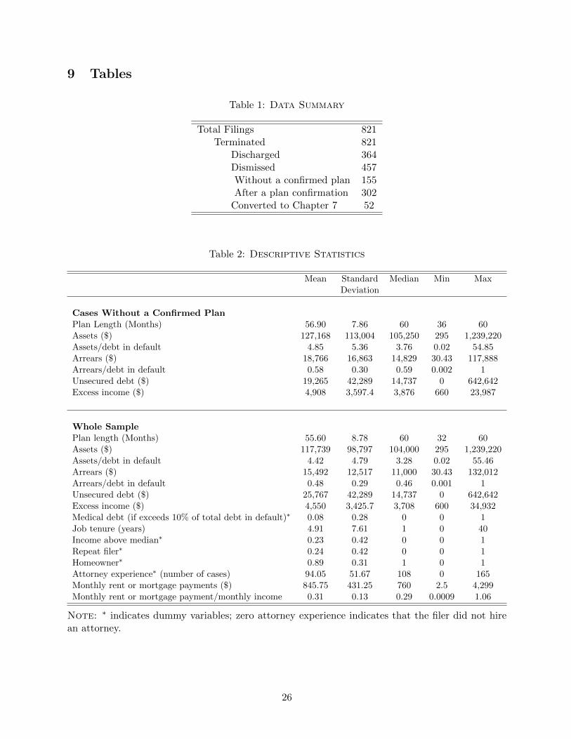
9 Tables

Table 1: Data Summary

Total Filings 821Terminated 821

Discharged 364Dismissed 457Without a confirmed plan 155After a plan confirmation 302

Converted to Chapter 7 52

Table 2: Descriptive Statistics

Mean Standard Median Min MaxDeviation

Cases Without a Confirmed PlanPlan Length (Months) 56.90 7.86 60 36 60Assets ($) 127,168 113,004 105,250 295 1,239,220Assets/debt in default 4.85 5.36 3.76 0.02 54.85Arrears ($) 18,766 16,863 14,829 30.43 117,888Arrears/debt in default 0.58 0.30 0.59 0.002 1Unsecured debt ($) 19,265 42,289 14,737 0 642,642Excess income ($) 4,908 3,597.4 3,876 660 23,987

Whole SamplePlan length (Months) 55.60 8.78 60 32 60Assets ($) 117,739 98,797 104,000 295 1,239,220Assets/debt in default 4.42 4.79 3.28 0.02 55.46Arrears ($) 15,492 12,517 11,000 30.43 132,012Arrears/debt in default 0.48 0.29 0.46 0.001 1Unsecured debt ($) 25,767 42,289 14,737 0 642,642Excess income ($) 4,550 3,425.7 3,708 600 34,932Medical debt (if exceeds 10% of total debt in default)∗ 0.08 0.28 0 0 1Job tenure (years) 4.91 7.61 1 0 40Income above median∗ 0.23 0.42 0 0 1Repeat filer∗ 0.24 0.42 0 0 1Homeowner∗ 0.89 0.31 1 0 1Attorney experience∗ (number of cases) 94.05 51.67 108 0 165Monthly rent or mortgage payments ($) 845.75 431.25 760 2.5 4,299Monthly rent or mortgage payment/monthly income 0.31 0.13 0.29 0.0009 1.06

Note: ∗ indicates dummy variables; zero attorney experience indicates that the filer did not hirean attorney.

26

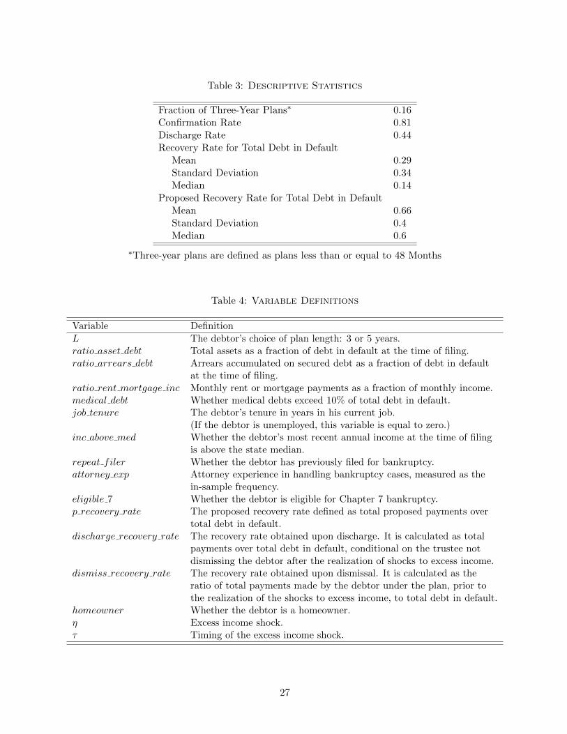
Table 3: Descriptive Statistics

Fraction of Three-Year Plans∗ 0.16Confirmation Rate 0.81Discharge Rate 0.44Recovery Rate for Total Debt in Default

Mean 0.29Standard Deviation 0.34Median 0.14

Proposed Recovery Rate for Total Debt in DefaultMean 0.66Standard Deviation 0.4Median 0.6

∗Three-year plans are defined as plans less than or equal to 48 Months

Table 4: Variable Definitions

Variable Definition

L The debtor’s choice of plan length: 3 or 5 years.ratio asset debt Total assets as a fraction of debt in default at the time of filing.ratio arrears debt Arrears accumulated on secured debt as a fraction of debt in default

at the time of filing.ratio rent mortgage inc Monthly rent or mortgage payments as a fraction of monthly income.medical debt Whether medical debts exceed 10% of total debt in default.job tenure The debtor’s tenure in years in his current job.

(If the debtor is unemployed, this variable is equal to zero.)inc above med Whether the debtor’s most recent annual income at the time of filing

is above the state median.repeat filer Whether the debtor has previously filed for bankruptcy.attorney exp Attorney experience in handling bankruptcy cases, measured as the

in-sample frequency.eligible 7 Whether the debtor is eligible for Chapter 7 bankruptcy.p recovery rate The proposed recovery rate defined as total proposed payments over

total debt in default.discharge recovery rate The recovery rate obtained upon discharge. It is calculated as total

payments over total debt in default, conditional on the trustee notdismissing the debtor after the realization of shocks to excess income.

dismiss recovery rate The recovery rate obtained upon dismissal. It is calculated as theratio of total payments made by the debtor under the plan, prior tothe realization of the shocks to excess income, to total debt in default.

homeowner Whether the debtor is a homeowner.η Excess income shock.τ Timing of the excess income shock.

27

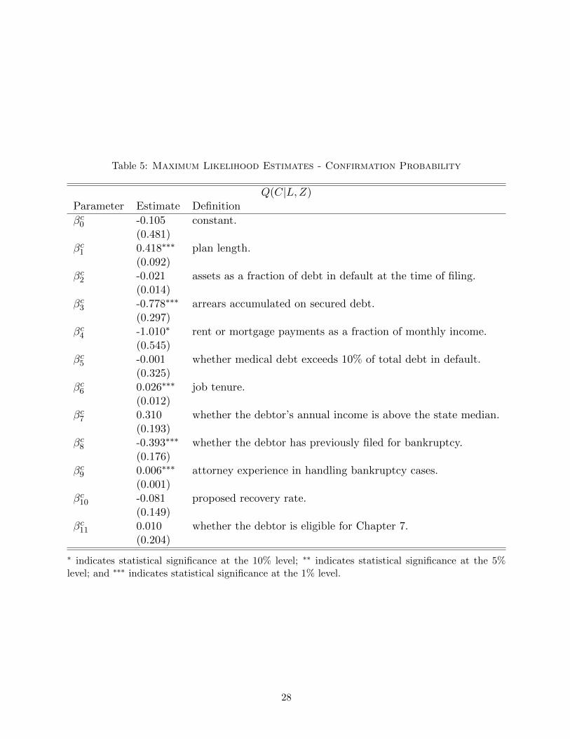
Table 5: Maximum Likelihood Estimates - Confirmation Probability

Q(C|L,Z)Parameter Estimate Definition

βc0 -0.105 constant.(0.481)

βc1 0.418∗∗∗ plan length.(0.092)

βc2 -0.021 assets as a fraction of debt in default at the time of filing.(0.014)

βc3 -0.778∗∗∗ arrears accumulated on secured debt.(0.297)

βc4 -1.010∗ rent or mortgage payments as a fraction of monthly income.(0.545)

βc5 -0.001 whether medical debt exceeds 10% of total debt in default.(0.325)

βc6 0.026∗∗∗ job tenure.(0.012)

βc7 0.310 whether the debtor’s annual income is above the state median.(0.193)

βc8 -0.393∗∗∗ whether the debtor has previously filed for bankruptcy.(0.176)

βc9 0.006∗∗∗ attorney experience in handling bankruptcy cases.(0.001)

βc10 -0.081 proposed recovery rate.(0.149)

βc11 0.010 whether the debtor is eligible for Chapter 7.(0.204)

∗ indicates statistical significance at the 10% level; ∗∗ indicates statistical significance at the 5%level; and ∗∗∗ indicates statistical significance at the 1% level.

28

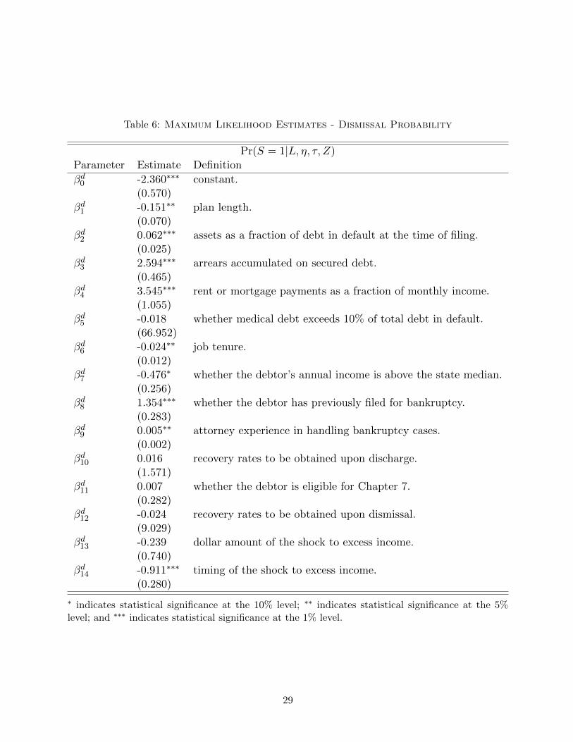
Table 6: Maximum Likelihood Estimates - Dismissal Probability

Pr(S = 1|L, η, τ, Z)Parameter Estimate Definition

βd0 -2.360∗∗∗ constant.(0.570)

βd1 -0.151∗∗ plan length.(0.070)

βd2 0.062∗∗∗ assets as a fraction of debt in default at the time of filing.(0.025)

βd3 2.594∗∗∗ arrears accumulated on secured debt.(0.465)

βd4 3.545∗∗∗ rent or mortgage payments as a fraction of monthly income.(1.055)

βd5 -0.018 whether medical debt exceeds 10% of total debt in default.(66.952)

βd6 -0.024∗∗ job tenure.(0.012)

βd7 -0.476∗ whether the debtor’s annual income is above the state median.(0.256)

βd8 1.354∗∗∗ whether the debtor has previously filed for bankruptcy.(0.283)

βd9 0.005∗∗ attorney experience in handling bankruptcy cases.(0.002)

βd10 0.016 recovery rates to be obtained upon discharge.(1.571)

βd11 0.007 whether the debtor is eligible for Chapter 7.(0.282)

βd12 -0.024 recovery rates to be obtained upon dismissal.(9.029)

βd13 -0.239 dollar amount of the shock to excess income.(0.740)

βd14 -0.911∗∗∗ timing of the shock to excess income.(0.280)

∗ indicates statistical significance at the 10% level; ∗∗ indicates statistical significance at the 5%level; and ∗∗∗ indicates statistical significance at the 1% level.

29

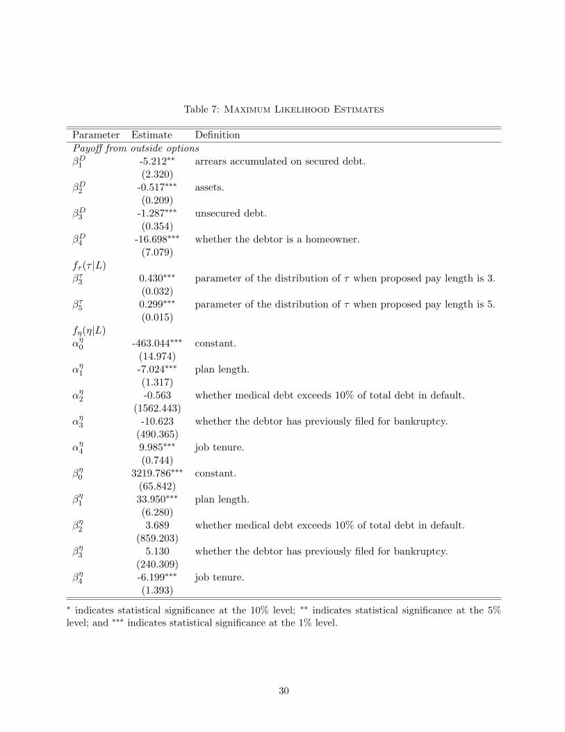
Table 7: Maximum Likelihood Estimates

Parameter Estimate Definition

Payoff from outside optionsβD1 -5.212∗∗ arrears accumulated on secured debt.

(2.320)βD2 -0.517∗∗∗ assets.

(0.209)βD3 -1.287∗∗∗ unsecured debt.

(0.354)βD4 -16.698∗∗∗ whether the debtor is a homeowner.

(7.079)fτ (τ |L)βτ3 0.430∗∗∗ parameter of the distribution of τ when proposed pay length is 3.

(0.032)βτ5 0.299∗∗∗ parameter of the distribution of τ when proposed pay length is 5.

(0.015)fη(η|L)αη0 -463.044∗∗∗ constant.

(14.974)αη1 -7.024∗∗∗ plan length.

(1.317)αη2 -0.563 whether medical debt exceeds 10% of total debt in default.

(1562.443)αη3 -10.623 whether the debtor has previously filed for bankruptcy.

(490.365)αη4 9.985∗∗∗ job tenure.

(0.744)βη0 3219.786∗∗∗ constant.

(65.842)βη1 33.950∗∗∗ plan length.

(6.280)βη2 3.689 whether medical debt exceeds 10% of total debt in default.

(859.203)βη3 5.130 whether the debtor has previously filed for bankruptcy.

(240.309)βη4 -6.199∗∗∗ job tenure.

(1.393)

∗ indicates statistical significance at the 10% level; ∗∗ indicates statistical significance at the 5%level; and ∗∗∗ indicates statistical significance at the 1% level.

30

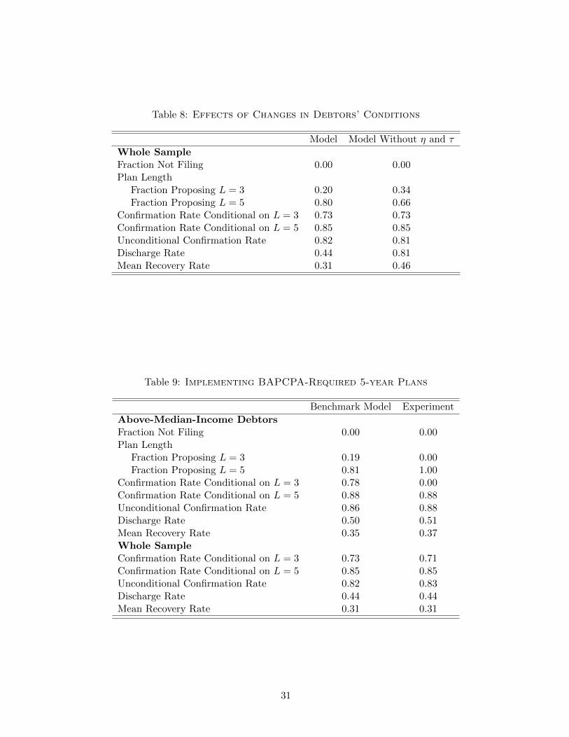
Table 8: Effects of Changes in Debtors’ Conditions

Model Model Without η and τ

Whole SampleFraction Not Filing 0.00 0.00Plan Length

Fraction Proposing L = 3 0.20 0.34Fraction Proposing L = 5 0.80 0.66

Confirmation Rate Conditional on L = 3 0.73 0.73Confirmation Rate Conditional on L = 5 0.85 0.85Unconditional Confirmation Rate 0.82 0.81Discharge Rate 0.44 0.81Mean Recovery Rate 0.31 0.46

Table 9: Implementing BAPCPA-Required 5-year Plans

Benchmark Model Experiment

Above-Median-Income DebtorsFraction Not Filing 0.00 0.00Plan Length

Fraction Proposing L = 3 0.19 0.00Fraction Proposing L = 5 0.81 1.00

Confirmation Rate Conditional on L = 3 0.78 0.00Confirmation Rate Conditional on L = 5 0.88 0.88Unconditional Confirmation Rate 0.86 0.88Discharge Rate 0.50 0.51Mean Recovery Rate 0.35 0.37Whole SampleConfirmation Rate Conditional on L = 3 0.73 0.71Confirmation Rate Conditional on L = 5 0.85 0.85Unconditional Confirmation Rate 0.82 0.83Discharge Rate 0.44 0.44Mean Recovery Rate 0.31 0.31

31

Table 10: Imposing a 30% Recovery Rate Threshold

Benchmark Model Experiment

Above-Median-Income DebtorsFraction Not Filing 0.00 0.26Plan Length

Fraction Proposing L = 3 0.19 0.10Fraction Proposing L = 5 0.81 0.64

Confirmation Rate Conditional on L = 3 0.78 0.76Confirmation Rate Conditional on L = 5 0.88 0.88Unconditional Confirmation Rate 0.86 0.64Discharge Rate 0.50 0.37Mean Recovery Rate 0.35 0.28Whole SampleConfirmation Rate Conditional on L = 3 0.73 0.72Confirmation Rate Conditional on L = 5 0.85 0.85Unconditional Confirmation Rate 0.82 0.66Discharge Rate 0.44 0.36Mean Recovery Rate 0.31 0.25

Table 11: Imposing a 30% Recovery Rate Threshold - Outside Recovery

Outside Recovery Rate: 0.10 Outside Recovery Rate: 0.20Benchmark Model Experiment Benchmark Model Experiment

Above-Median-Income DebtorsFraction Not Filing 0.00 0.26 0.00 0.26Initial Dismissal Rate Conditional on

L = 3 0.22 0.24 0.21 0.24L = 5 0.12 0.12 0.12 0.12

Unconditional Initial Dismissal Rate 0.24 0.36 0.24 0.36Dismissed after Confirmation 0.36 0.27 0.36 0.27Mean Recovery Rate

Under Chapter 13 0.35 0.28 0.35 0.28Overall 0.38 0.33 0.42 0.39

Whole SampleOverall Mean Recovery Rate 0.34 0.30 0.39 0.36

32

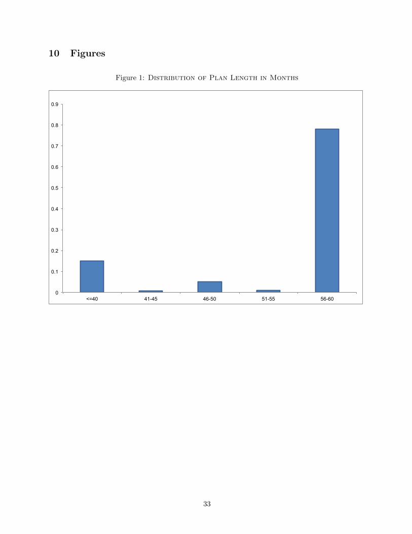
10 Figures

Figure 1: Distribution of Plan Length in Months

0

0.1

0.2

0.3

0.4

0.5

0.6

0.7

0.8

0.9

<=40 41-45 46-50 51-55 56-60

33

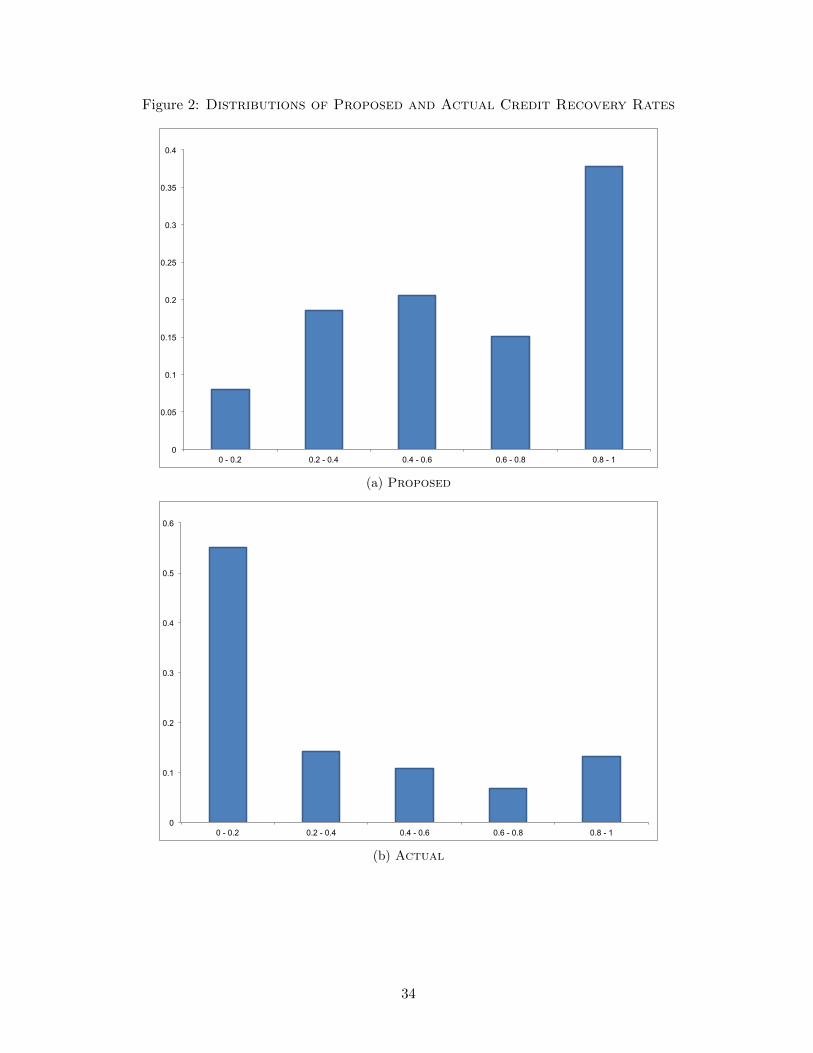
Figure 2: Distributions of Proposed and Actual Credit Recovery Rates

0

0.05

0.1

0.15

0.2

0.25

0.3

0.35

0.4

0 - 0.2 0.2 - 0.4 0.4 - 0.6 0.6 - 0.8 0.8 - 1

(a) Proposed

0

0.1

0.2

0.3

0.4

0.5

0.6

0 - 0.2 0.2 - 0.4 0.4 - 0.6 0.6 - 0.8 0.8 - 1

(b) Actual

34

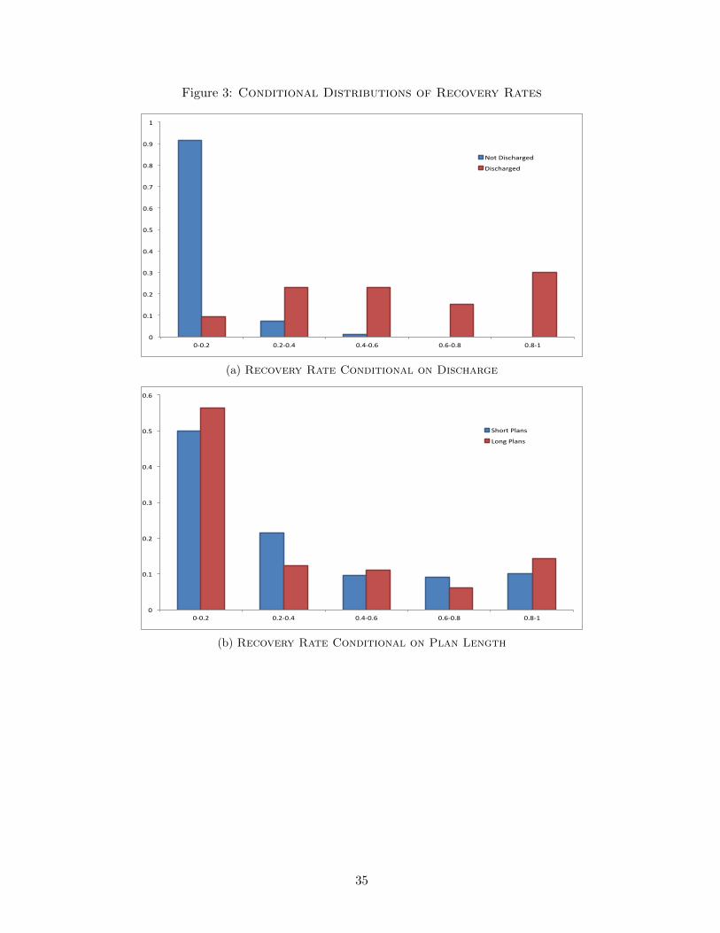
Figure 3: Conditional Distributions of Recovery Rates

0  

0.1  

0.2  

0.3  

0.4  

0.5  

0.6  

0.7  

0.8  

0.9  

1  

0-­‐0.2   0.2-­‐0.4   0.4-­‐0.6   0.6-­‐0.8   0.8-­‐1  

Not  Discharged  

Discharged  

(a) Recovery Rate Conditional on Discharge

0  

0.1  

0.2  

0.3  

0.4  

0.5  

0.6  

0-­‐0.2   0.2-­‐0.4   0.4-­‐0.6   0.6-­‐0.8   0.8-­‐1  

Short  Plans  

Long  Plans  

(b) Recovery Rate Conditional on Plan Length

35

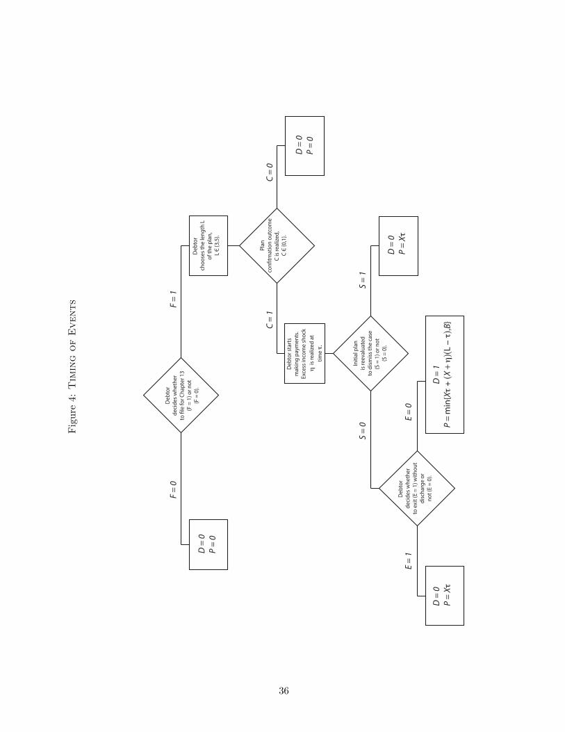
Fig

ure

4:T

imin

gof

Events

D =

0P

= 0

Plan

con�

tmat

ion

outc

ome

C is

real

ized

, C

Є {0

,1}.

Deb

tor

deci

des w

heth

er

to �

le fo

r Cha

pter

13

(F =

1) o

r not

(F

= 0

).

F =

0F

= 1

Deb

tor

choo

ses t

he le

ngth

Lof

the

plan

, L

Є {3

,5}.

C =

0C

= 1

D =

0P

= 0

Deb

tor s

tart

s m

akin

g pa

ymen

ts.

Exce

ss in

com

e sh

ock

η i

s rea

lized

at

time

τ.

Initi

al p

lan

is re

eval

uate

dto

dis

mis

s the

cas

e(S

= 1

) or n

ot

(S =

0).

S =

1

D =

0P

= X

τD

ebto

r de

cide

s whe

ther

to e

xit (

E =

1) w

ithou

tdi

scha

rge

orno

t (E

= 0)

.

S =

0

E =

1

D =

0 P

= X

τ

E =

0

D =

1P

= m

in{X

τ +

(X +

η)(

L −

τ),B

}

36

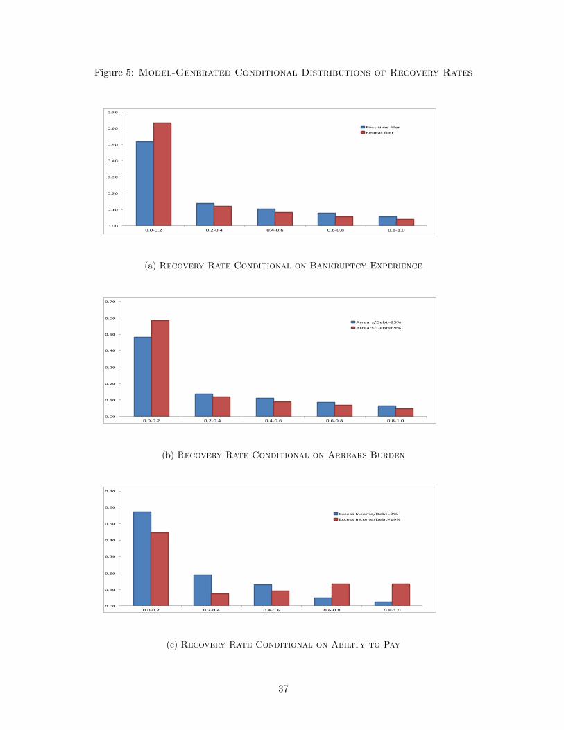
Figure 5: Model-Generated Conditional Distributions of Recovery Rates

0.00

0.10

0.20

0.30

0.40

0.50

0.60

0.70

0.0-0.2 0.2-0.4 0.4-0.6 0.6-0.8 0.8-1.0

First-2mefiler

Repeatfiler

(a) Recovery Rate Conditional on Bankruptcy Experience

0.00

0.10

0.20

0.30

0.40

0.50

0.60

0.70

0.0-0.2 0.2-0.4 0.4-0.6 0.6-0.8 0.8-1.0

Arrears/Debt=25%

Arrears/Debt=69%

(b) Recovery Rate Conditional on Arrears Burden

0.00

0.10

0.20

0.30

0.40

0.50

0.60

0.70

0.0-0.2 0.2-0.4 0.4-0.6 0.6-0.8 0.8-1.0

ExcessIncome/Debt=8%

ExcessIncome/Debt=19%

(c) Recovery Rate Conditional on Ability to Pay

37

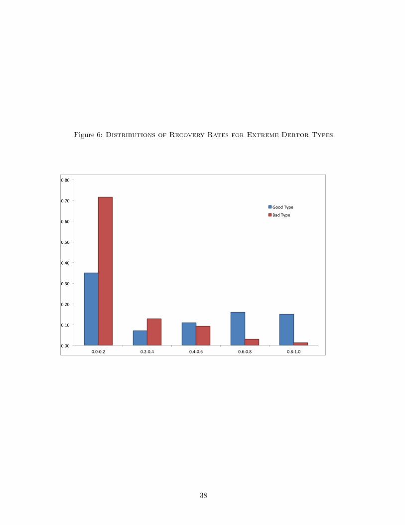
Figure 6: Distributions of Recovery Rates for Extreme Debtor Types

0.00

0.10

0.20

0.30

0.40

0.50

0.60

0.70

0.80

0.0-0.2 0.2-0.4 0.4-0.6 0.6-0.8 0.8-1.0

GoodType

BadType

38

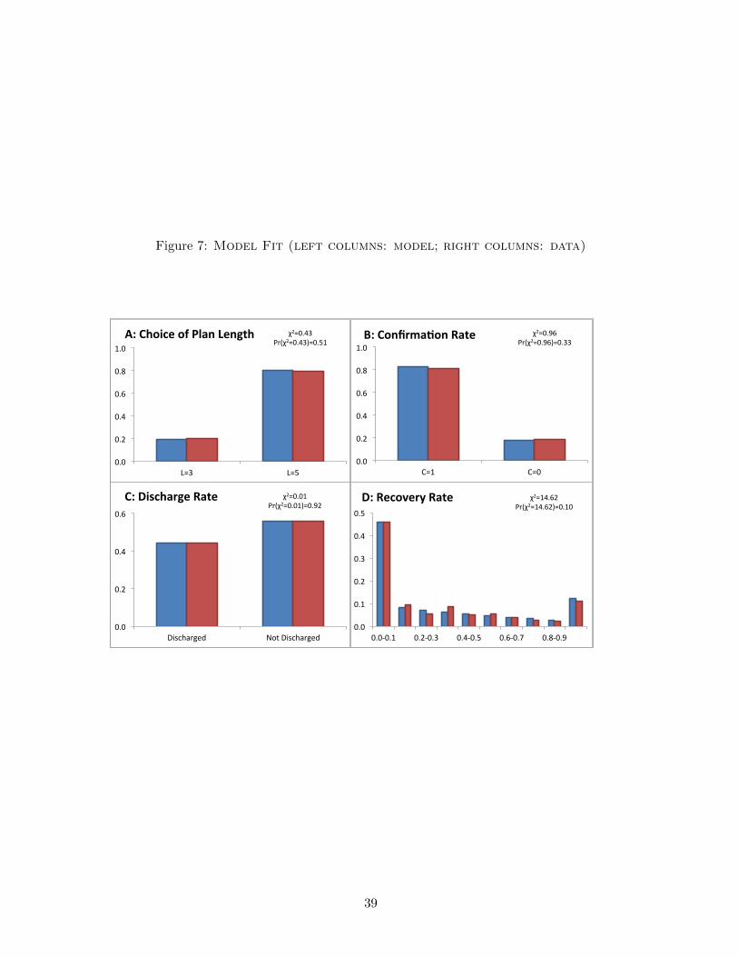
Figure 7: Model Fit (left columns: model; right columns: data)

0.0

0.2

0.4

0.6

0.8

1.0

L=3 L=5

A:ChoiceofPlanLength χ2=0.43Pr(χ2=0.43)=0.51

0.0

0.2

0.4

0.6

Discharged NotDischarged

C:DischargeRate χ2=0.01Pr(χ2=0.01)=0.92

0.0

0.2

0.4

0.6

0.8

1.0

C=1 C=0

B:Confirma9onRate χ2=0.96Pr(χ2=0.96)=0.33

0.0

0.1

0.2

0.3

0.4

0.5

0.0-0.1 0.2-0.3 0.4-0.5 0.6-0.7 0.8-0.9

D:RecoveryRate χ2=14.62Pr(χ2=14.62)=0.10

39