7/28/’10

UseR! The R User Conference 2010

An Algorithm for Unconstrained

Quadratically Penalized Convex

Optimization (post conference

version)

Steven P. EllisNew York State Psychiatric Institute

at Columbia University

PROBLEM

Minimize functions of form

F (h) = V (h) +Q(h), h ∈ Rd,

1. (R = reals; d = positive integer.)

2. V is non-negative and convex.

3. V is computationally expensive.

4. Q is known, strictly convex, and quadratic.

5. (Unconstrained optimization problem)

6. Gradient, but not necessarily Hessian are available.

NONPARAMETRIC FUNCTION ESTIMATION

• Need to minimize:

F (h) = V (h) + λhTQh.

– λ > 0 is “complexity parameter”.

WAR STORY

• Work on a kernel-based survival analysis algorithm

lead me to work on this optimization problem.

• At first I used BFGS, but it was very slow.

– (Broyden, ’70; Fletcher, ’70; Goldfarb, ’70; Shanno,

’70)

– Once I waited 19 hours for it to converge!

• Finding no software for unconstrained convex opti-

mization (see below), I invented my own.

SOFTWARE FOR UNCONSTRAINED CONVEX OP-

TIMIZATION

Didn’t find such software.

• CVX ( http://cvxr.com/cvx/ ) is a Matlab-based

modeling system for convex optimization.

– But a developer, Michael Grant, says that CVX

wasn’t designed for problems such as my survival

analysis problem.

“QQMM”

• Developed algorithm “QQMM” (“quasi-quadratic

minimization with memory”; Q2M2) to solve prob-

lems of this type.

– Implemented in R.

– Posted on STATLIB.

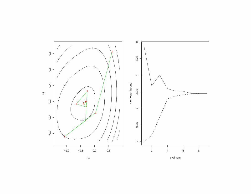
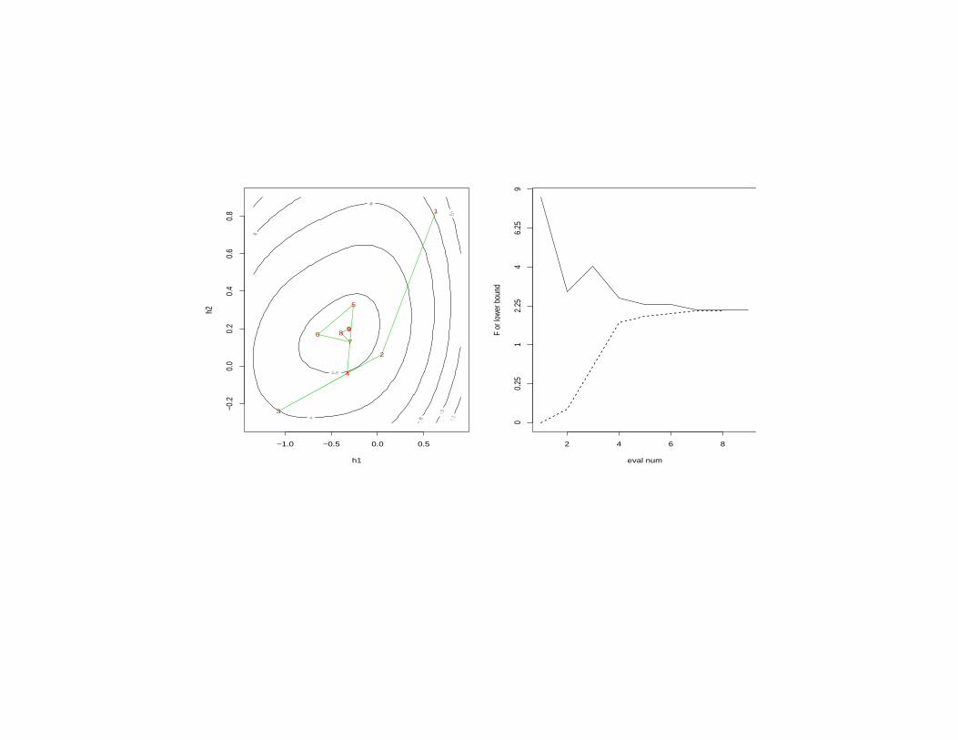
Iterative descent method

• An iteration: If h1 ∈ Rd has smallest F value found

so far, compute one or more trial minimizers, h2,

until “sufficient decrease” is achieved.

• Assign h2 → h1 to finish iteration.

• Repeat until evaluation limit is exceeded or stopping

criteria are met.

h1

h2

−1.0 −0.5 0.0 0.5

−0

.20

.00

.20

.40

.60

.81

2

3

4

5

67

899

eval num

F o

r lo

we

r b

ou

nd

2 4 6 8

00

.25

12

.25

46

.25

9

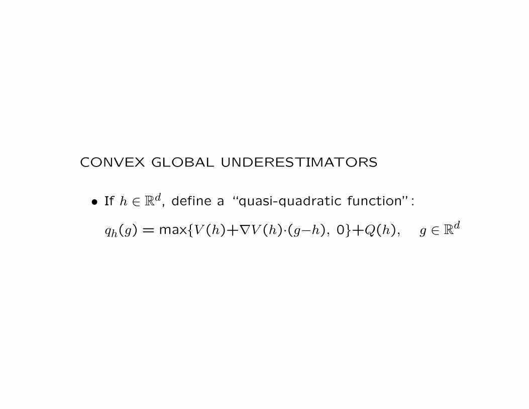
CONVEX GLOBAL UNDERESTIMATORS

• If h ∈ Rd, define a “quasi-quadratic function”:

qh(g) = max{V (h)+∇V (h)·(g−h), 0}+Q(h), g ∈ Rd

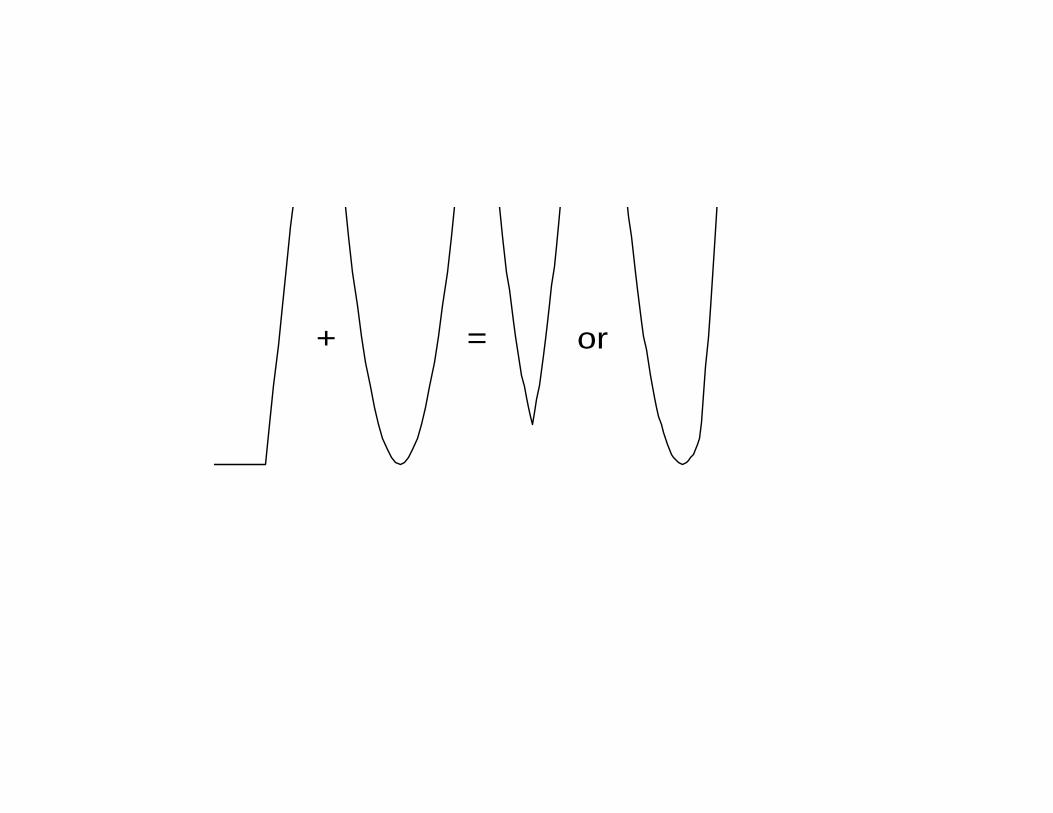
+ = or

• qh is a convex “global underestimator” of F :

qh ≤ F.

• Possible trial minimand of F is the point h2 where

qh is minimum, but that doesn’t work very well.

L.U.B.’S

• If h(1), . . . h(n) ∈ Rd are points visited by algorithmso far, the least upper bound (l.u.b.) of

qh(1), qh(2)

, . . . , qh(n−1), qh(n)

is their pointwise maximum:

Fn(h) = max{qh(1)(h), qh(2)

(h), . . . , qh(n−1)(h), qh(n)

(h)},

• Fn is also a convex global underestimator of F nosmaller than any qh(i)

.

• The point, h2 where Fn is minimum is probably agood trial minimizer.

• But minimizing Fn may be at least as hard as min-imizing F !

• As a compromise, proceed as follows.

– Let h1 = h(n) be best trial minimizer found so

far and let h(1), . . . h(n) ∈ R be points visited by

algorithm so far.

• – For i = 1,2, . . . , n− 1 let qh(i),h1be l.u.b. of qh(i)

and qh1.

∗ “q double h”

∗ Convex global underestimator of F .

∗ Easy to minimize in closed form.

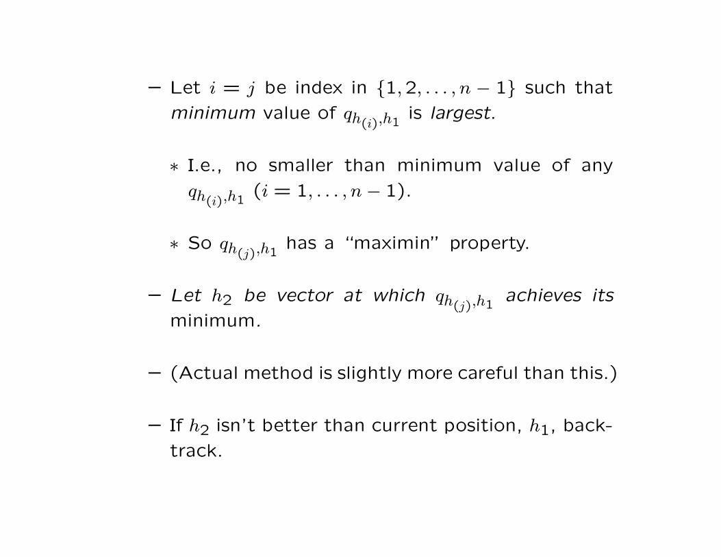
– Let i = j be index in {1,2, . . . , n − 1} such that

minimum value of qh(i),h1is largest.

∗ I.e., no smaller than minimum value of any

qh(i),h1(i = 1, . . . , n− 1).

∗ So qh(j),h1has a “maximin” property.

– Let h2 be vector at which qh(j),h1achieves its

minimum.

– (Actual method is slightly more careful than this.)

– If h2 isn’t better than current position, h1, back-

track.

Minimizing qh(i),h1requires matrix operations.

• Limits size of problems for which Q2M2 can be used

to no more than, say, 4 or 5 thousand variables.

STOPPING RULE

• Trial values h2 are minima of nonnegative global

underestimators of F .

• Values of these global underestimators at corre-

sponding h2’s are lower bounds on minF .

• Store cumulative maxima of these lower bounds.

– Let L denote current value of cumulative maxi-

mum.

– L is a lower bound on minF .

• If h1 is current best trial minimizer, relative differ-

ence between F (h1) and L exceeds relative differ-

ence between F (h1) and minF .

F (h1)− LL

≥F (h1)−minF

minF.

• I.e., we can explicitly bound relative error in F (h1)

as an estimate of minF !

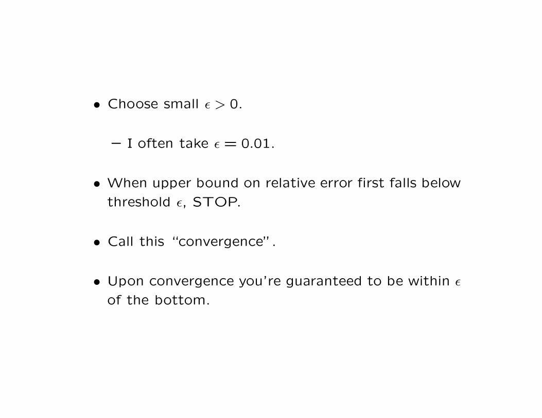
• Choose small ε > 0.

– I often take ε = 0.01.

• When upper bound on relative error first falls below

threshold ε, STOP.

• Call this “convergence”.

• Upon convergence you’re guaranteed to be within ε

of the bottom.

h1

h2

−1.0 −0.5 0.0 0.5

−0.2

0.0

0.2

0.4

0.6

0.8 1

2

3

4

5

67

899

eval num

F or

lowe

r bou

nd

2 4 6 8

00.

251

2.25

46.

259

• Gives good control over stopping.

• That is important because . . .

STOPPING EARLY MAKES SENSE IN STATISTICAL

ESTIMATION

• In statistical estimation, the function, F , depends,

through V , on noisy data so:

• In statistical estimation there’s no point in taking

time to achieve great accuracy in optimization.

•

F (h) = V (h) +Q(h), h ∈ Rd,

Q2M2 IS SOMETIMES SLOW

• Q2M2 tends to close in on minimum rapidly.

• But sometimes is very slow to converge.

– E.g., when Q is nearly singular.

– E.g., when complexity parameter, λ, is small.

• Distribution of number of evaluations needed for

convergence has long right hand tail as you vary

over optimization problems.

SIMULATIONS: “PHILOSOPHY”

• If F is computationally expensive then simulations

are unworkable.

• A short computation time for optimizations is de-

sired.

• When F is computationally expensive then compu-

tation time is roughly proportional to number of

function evaluations.

• Simulate computationally cheap F ’s, but track num-

ber of evaluations not computation time.

COMPARE Q2M2 AND BFGS.

• Why BFGS?

– BFGS is widely used.

∗ “Default” method

– Like Q2M2, BFGS uses gradient and employs

vector-matrix operations.

– Optimization maven at NYU (Michael Overton)

suggested it as comparator!

– (Specifically, the “BFGS” option in the R func-

tion optim that was used. John C. Nash – per-

sonal communication – pointed out at the con-

ference that other algorithms called “BFGS” are

faster than the BFGS in optim.)

SIMULATION STRUCTURE

• I chose several relevant estimation problems.

• For each of variety of choices of complexity param-

eter λ use both Q2M2 and BFGS to fit model to

randomly generated training sample and test data.

– Either simulated data or real data randomly split

into two subsamples.

• Repeat 1000 times for each choice of λ.

• Gather numbers of evaluations required and other

statistics describing simulations.

• Use

Gibbons, Olkin, Sobel (’99) Selecting and Or-

dering Populations: A New Statistical Method-

ology

to select the range of λ values that, with 95% con-

fidence, contains λ with lowest mean test error.

• Conservative to use largest λ in selected group.

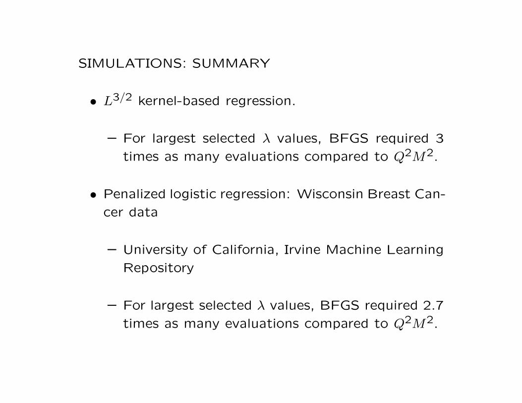
SIMULATIONS: SUMMARY

• L3/2 kernel-based regression.

– For largest selected λ values, BFGS required 3

times as many evaluations compared to Q2M2.

• Penalized logistic regression: Wisconsin Breast Can-

cer data

– University of California, Irvine Machine Learning

Repository

– For largest selected λ values, BFGS required 2.7

times as many evaluations compared to Q2M2.

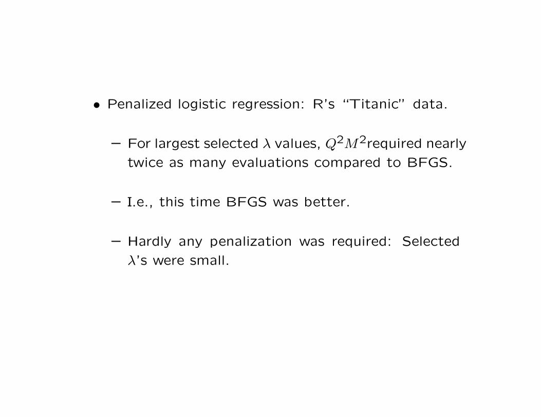
• Penalized logistic regression: R’s “Titanic” data.

– For largest selected λ values, Q2M2required nearly

twice as many evaluations compared to BFGS.

– I.e., this time BFGS was better.

– Hardly any penalization was required: Selected

λ’s were small.

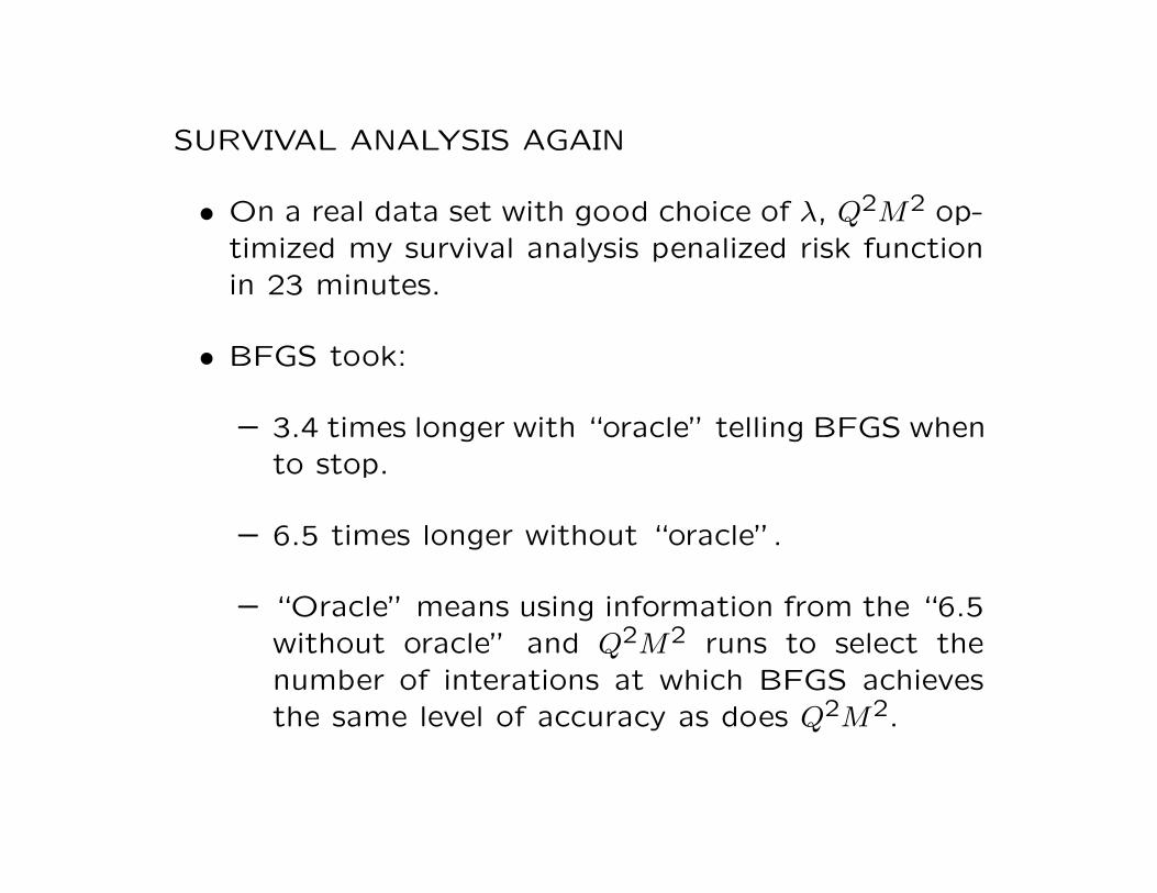
SURVIVAL ANALYSIS AGAIN

• On a real data set with good choice of λ, Q2M2 op-timized my survival analysis penalized risk functionin 23 minutes.

• BFGS took:

– 3.4 times longer with “oracle” telling BFGS whento stop.

– 6.5 times longer without “oracle”.

– “Oracle” means using information from the “6.5without oracle” and Q2M2 runs to select thenumber of interations at which BFGS achievesthe same level of accuracy as does Q2M2.

CONCLUSIONS

• QQMM (Q2M2) is an algorithm for minimizing con-

vex functions of form

F (h) = V (h) +Q(h), h ∈ Rd.

– V is convex and non-negative.

– Q is known, quadratic, strictly convex.

– Q2M2 is especially appropriate when V is expen-

sive to compute.

• Allows good control of stopping.

• Needs (sub)gradient.

• Utilizes matrix algebra. This limits maximum size of

problems to no more than 4 or 5 thousand variables.

• Q2M2 is often quite fast, but can be slow if Q is

nearly singular.