an abstract of the thesis of - college of...
TRANSCRIPT


AN ABSTRACT OF THE THESIS OF
Kevin J. Drost for the degree of Master of Science in Mechanical Engineering and
Environmental Geology presented on June 4, 2012.
Title: RANS and LES Predictions of Turbulent Scalar Transport in Dead Zones
of Natural Streams
Abstract approved:
Sourabh V. Apte Roy Haggerty
Natural stream systems contain a variety of flow geometries which contain flow
separation, turbulent shear layers, and recirculation zones. This work focuses on
streams with dead zones. Characterized by slower flow and recirculation, dead
zones are naturally occurring cutouts in stream banks. These dead zones play an
important role in stream nutrient retention and solute transport. Previous exper-
imental work has focused on idealized dead zone geometries studied in laboratory
flumes. This work explores the capabilities of computational fluid dynamics (CFD)
to investigate the scaling relationships between flow parameters of idealized geome-
tries and the time scales of transport. The stream geometry can be split into two
main regions, the main stream flow and the dead zone. Geometric parameters of
the dead zone as well as the bulk stream velocity were varied to determine a scal-
ing relationship for the transport time scales. These flow geometries are simulated

using the RANS turbulence model with the standard k-ω closure. The standard
first order dead zone model is expanded to a two region model to accommodate the
multiple time scales observed in the simulation results. While this model currently
has limited predictive capability, it provides physical insight into the functional
dependence of the dead zone time scales. LES is used to evaluate the performance
of the Reynolds Averaged Navier-Stokes (RANS) turbulence model and to describe
the anisotropic turbulence characteristics. The differences between the time av-
eraged flow field for Large Eddy Simulation (LES) and RANS was determined to
have a significant impact on passive scalar transport.

c©Copyright by Kevin J. DrostJune 4, 2012
All Rights Reserved

RANS and LES Predictions of Turbulent Scalar Transport in DeadZones of Natural Streams
by
Kevin J. Drost
A THESIS
submitted to
Oregon State University
in partial fulfillment ofthe requirements for the
degree of
Master of Science
Presented June 4, 2012Commencement June 2012

Master of Science thesis of Kevin J. Drost presented on June 4, 2012.
APPROVED:
Co-Major Professor, representing Mechanical Engineering
Co-Major Professor, representing Environmental Geology
Head of the School of Mechanical, Industrial, and Manufacturing Engineering
Dean of the Graduate School
I understand that my thesis will become part of the permanent collection ofOregon State University libraries. My signature below authorizes release of mythesis to any reader upon request.
Kevin J. Drost, Author

ACKNOWLEDGEMENTS
I would like to acknowledge Dr. Sourabh Apte for his patient guidance. Whenever
I faced a challenge in my research, he would offer advice, an encouraging word, or
ask the right questions to keep me on task and moving forward. I would also like
to thank the other members of this project, Dr. Roy Haggerty and Tracie Jackson
for their professional, kind, and intelligent discussions throughout the research
process. Lab mates Justin Finn and Andrew Cihonski also contributed guidance
and helped with many of the technical details of this work. Additionally, I would
like to thank my family for their constant loving support. Through countless ways,
they have shaped me and encouraged me throughout my education. I would also
like to to thank my friends and roommates for patiently listening to my research
struggles and reminding me there is more to graduate school than the work.

TABLE OF CONTENTS
Page
1 Introduction 2
2 Literature Review 6
2.1 Dead Zones . . . . . . . . . . . . . . . . . . . . . . . . . . . . . . . . 6
2.2 Numerical Techniques . . . . . . . . . . . . . . . . . . . . . . . . . . 9
3 Mathematical Formulation 12
3.1 Dimensional Analysis . . . . . . . . . . . . . . . . . . . . . . . . . . . 12
3.2 Governing Equations . . . . . . . . . . . . . . . . . . . . . . . . . . . 14
3.3 RANS Turbulence Model . . . . . . . . . . . . . . . . . . . . . . . . . 15
3.4 LES Turbulence Model . . . . . . . . . . . . . . . . . . . . . . . . . . 19
4 Dead Zone Models 25
4.1 First Order Model . . . . . . . . . . . . . . . . . . . . . . . . . . . . 26
4.2 Two Region Model . . . . . . . . . . . . . . . . . . . . . . . . . . . . 28
4.3 Model Fitting . . . . . . . . . . . . . . . . . . . . . . . . . . . . . . . 32
4.4 Important Time Scales . . . . . . . . . . . . . . . . . . . . . . . . . . 33
5 RANS Cases 35
5.1 Solution Procedure . . . . . . . . . . . . . . . . . . . . . . . . . . . . 35
5.2 Series Geometry and Grids . . . . . . . . . . . . . . . . . . . . . . . . 36
5.3 Series Validation . . . . . . . . . . . . . . . . . . . . . . . . . . . . . 40
5.4 Series Results . . . . . . . . . . . . . . . . . . . . . . . . . . . . . . . 45
5.5 Single Geometry and Grid . . . . . . . . . . . . . . . . . . . . . . . . 48
5.6 Single Dead Zone Results . . . . . . . . . . . . . . . . . . . . . . . . 50
5.7 Two Region Model . . . . . . . . . . . . . . . . . . . . . . . . . . . . 56
6 LES Cases 60
6.1 Geometry and Grids . . . . . . . . . . . . . . . . . . . . . . . . . . . 60
6.2 Solution Procedure . . . . . . . . . . . . . . . . . . . . . . . . . . . . 61

TABLE OF CONTENTS (Continued)
Page
6.3 LES Results . . . . . . . . . . . . . . . . . . . . . . . . . . . . . . . . 63
7 Conclusions 70
Bibliography 72
Appendices 78

LIST OF FIGURES
Figure Page
1.1 Schematic of a typical dead zone showing the mixing layer andstreamwise velocity profile. W is measured in the spanwise direc-tion. L is measured in the streamwise direction. . . . . . . . . . . . 4
1.2 A natural dead zone caused by an obstruction in a stream. Themain channel flow is from right to left. . . . . . . . . . . . . . . . . 4
3.1 Plan view and cross section of a simplified dead zone with the stan-dard dimensions labeled. . . . . . . . . . . . . . . . . . . . . . . . . 13
3.2 Conceptualization of the energy cascade of the turbulent energycontent of a flow as a function of the wavenumber. . . . . . . . . . . 20
4.1 A comparison plan views of the two ways dead zones are formedviewed from the top. Top: Dead zone is formed by a cutout intothe bank, Bottom: Dead zone is formed by obstructions in the mainchannel. . . . . . . . . . . . . . . . . . . . . . . . . . . . . . . . . . 26
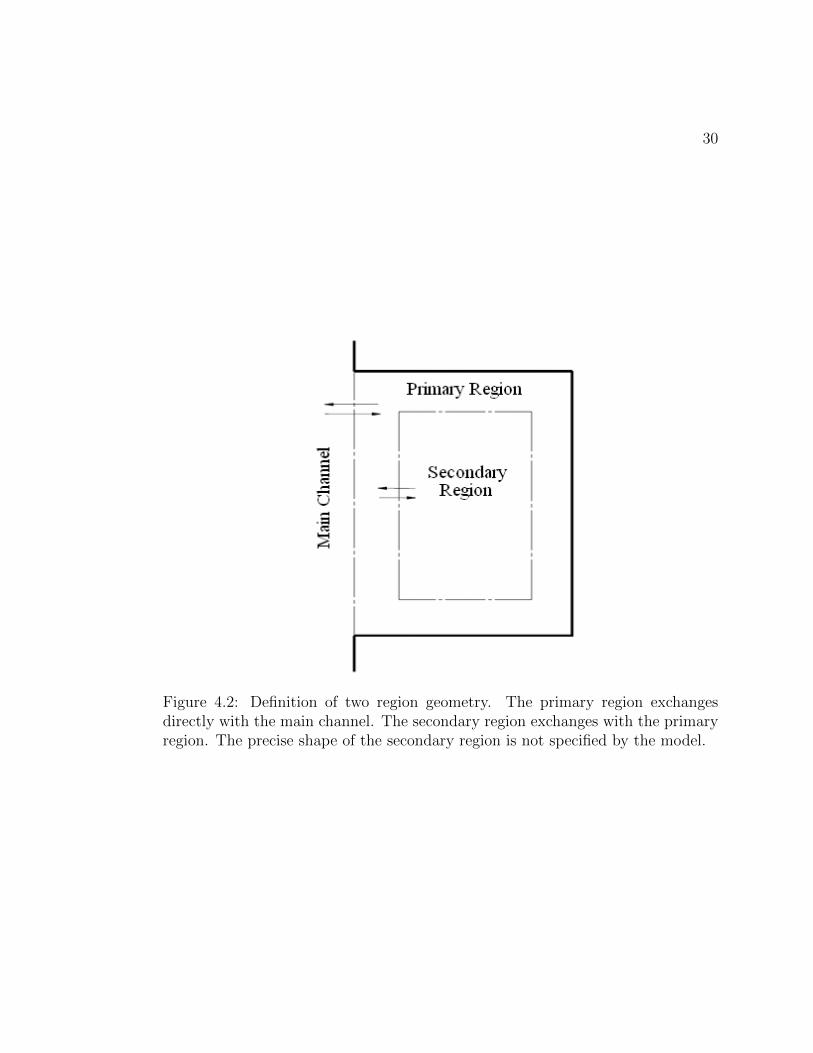
4.2 Definition of two region geometry. The primary region exchangesdirectly with the main channel. The secondary region exchangeswith the primary region. The precise shape of the secondary regionis not specified by the model. . . . . . . . . . . . . . . . . . . . . . 30
5.1 Description of the geometry for a series of six dead zones matchingexperiments done by Uijttewaal [41]. Top: Plan view of geometry.Bottom: Cross section of geometry. . . . . . . . . . . . . . . . . . . 38
5.2 Description of the geometry for a series of dead zones matchingexperiments done by Weitbrecht [46]. This geometry has a uniformdepth. . . . . . . . . . . . . . . . . . . . . . . . . . . . . . . . . . . 40
5.3 Streamwise velocity profile in the spanwise direction for the baseand refined grids. Velocity is taken at the free surface and on thecenterline of the 5th dead zone in the series using the Uijttewaalgeometry. . . . . . . . . . . . . . . . . . . . . . . . . . . . . . . . . 41
5.4 TKE profile in the spanwise direction for the base and refined grids.TKE is taken at the free surface and on the centerline of the 5thdead zone in the series using the Uijttewaal geometry. . . . . . . . . 42

LIST OF FIGURES (Continued)
Figure Page
5.5 Streamwise velocity profile in the spanwise direction for the Uijt-tewaal geometry comparing the current RANS simulations, experi-mental work by Uijttewaal et al. [41], and simulations by McCoy etal. [30]. All data is collected at the free surface and X=6 m (in the6th dead zone). . . . . . . . . . . . . . . . . . . . . . . . . . . . . . 43
5.6 TKE profile in the spanwise direction for the Uijttewaal geometrycomparing the current RANS simulations, experimental work byUijttewaal et al. [41], and simulations by McCoy et al. [30]. Alldata is collected at the free surface and X=6.1 m (in the 6th deadzone). . . . . . . . . . . . . . . . . . . . . . . . . . . . . . . . . . . 44
5.7 Flow quantities as a function of streamwise position for the refinedgrid. Data is collected at the free surface on the line that separatesthe dead zones from the main channel. The developing shear layeris shown for five dead zones. . . . . . . . . . . . . . . . . . . . . . . 46
5.8 Streamlines at the free surface in a dead zone after the shear layeris fully developed for two different average velocities using the Weit-brecht geometry. . . . . . . . . . . . . . . . . . . . . . . . . . . . . 47
5.9 Streamlines at the free surface in a dead zone after the shear layeris fully developed for three different lengths using the Weitbrechtgeometry. . . . . . . . . . . . . . . . . . . . . . . . . . . . . . . . . 47
5.10 Plot of the ratio of the Langmuir to convective time scales vs. theaspect ratio for series of dead zones. Experimental results fromUijttewaal et al. [41] and Weitbrecht et al. [46] are included. . . . . 48
5.11 Plan view of the single dead zone geometry. The depth is uniformin the main channel and dead zone. . . . . . . . . . . . . . . . . . . 49
5.12 Plot of the ratio of the Langmuir to convective time scales vs. theaspect ratio for single dead zone. Only cases varying L and W areshown. . . . . . . . . . . . . . . . . . . . . . . . . . . . . . . . . . . 51
5.13 Plot of the ratio of the Langmuir to convective time scales vs. an em-pirically derived nondimensional parameter that includes geometricand flow parameters. . . . . . . . . . . . . . . . . . . . . . . . . . . 53
LIST OF FIGURES (Continued)
Figure Page
5.14 Contour of the concentration within the dead zone for the base singledead zone case. The dark region represents higher concentration. . . 54
5.15 Plot of the normalized dead zone concentration vs. time for the basecase single dead zone geometry. . . . . . . . . . . . . . . . . . . . . 54
5.16 Plot of the instantaneous time scale, T , vs. time for the base singledead zone case. τL and T0 are shown for reference. . . . . . . . . . . 55
5.17 Plot of the dead zone concentration for the base single dead zonecase. Symbols are from fitting the two region model to the concen-tration plot. The average error between the two is 0.71%. . . . . . . 56
5.18 Three experimental concentration plots by Jackson et al. [14] fitwith the two region model. . . . . . . . . . . . . . . . . . . . . . . . 59
6.1 Plot comparing the streamwise velocity profile in the spanwise di-rection for both LES grids to a RANS simulation on the coarse grid.The dashed vertical line represents the main channel-dead zone in-terface. Data is collected at the free surface and on the X=0.4mline. . . . . . . . . . . . . . . . . . . . . . . . . . . . . . . . . . . . 63
6.2 Plot comparing the streamwise velocity profile in the spanwise direc-tion for this LES study, LES by McCoy et al. [30], and experimentsby Uijttewaal et al. [41]. The dashed vertical line represents themain channel-dead zone interface. Data is collected at the free sur-face and on the X=0.4m line. . . . . . . . . . . . . . . . . . . . . . 64
6.3 Average streamlines at the free surface in the dead zone for thecoarse LES grid. . . . . . . . . . . . . . . . . . . . . . . . . . . . . . 66
6.4 Contours of uzU
, the time averaged exchange velocity at the interfacebetween the dead zone and main channel for the coarse LES grid.The Y dimension is stretched by a factor of 10. . . . . . . . . . . . 66
6.5 Plan view contours of u′xu′x
U2 at the free surface for the coarse LES grid. 67
6.6 Plots of the normalized dead zone concentration vs. time for RANSscalar studies using the time average flow field from LES and RANS.Both simulations use the coarse LES grid. . . . . . . . . . . . . . . 68

LIST OF TABLES
Table Page
5.1 Base grid sizes, in meters and wall units, used in the shear layerand dead zone for the Uijttewaal geometry. There are different Yspacings for the main channel (MC) and the dead zone (DZ). . . . . 39
5.2 Refined grid sizes, in meters and wall units, used in the shear layerand dead zone for the Uijttewaal geometry. There are different Yspacings for the main channel (MC) and the dead zone (DZ). . . . . 39
5.3 Base grid sizes, in meters and wall units, used in the shear layer anddead zone for the Weitbrecht geometry. . . . . . . . . . . . . . . . . 40
5.4 Different dead zones parameters used in the single dead zone cases. 50
5.5 Results from fitting the two region model to the single dead zonecases. Model parameters τp, τs, and k3 are shown as well as theaverage percent error. . . . . . . . . . . . . . . . . . . . . . . . . . . 57
6.1 Grid spacings for the coarse and refined LES grids in the dead zoneand shear layer in meters and wall units. . . . . . . . . . . . . . . . 61
6.2 Two region parameters, τp, τs, and k3, fit to the concentration plotsfrom RANS passive scalar analyses using the mean flow field fromLES and RANS. The average percent error between model and sim-ulation is also shown. . . . . . . . . . . . . . . . . . . . . . . . . . . 69

LIST OF APPENDICES
Page
A k-ω Equations 79
B Uijttewaal Grids 81
C Weitbrecht Grids 82
D Single Grid 83
E LES Grid 85
F Additional LES Plots 87

LIST OF APPENDIX FIGURES
Figure Page
B.1 Cross section of the Uijttewaal grid. . . . . . . . . . . . . . . . . . . 81
B.2 Detailed plan view of the Uijttewaal grid used in a dead zone. . . . 81
C.1 Cross section of the Weitbrecht grid. . . . . . . . . . . . . . . . . . 82
C.2 Detailed plan view of the Weitbrecht grid used in the dead zone. . . 82
D.1 Cross section of the single geometry grid. . . . . . . . . . . . . . . . 83
D.2 Detailed view of the cross section of the dead zone corner for thesingle geometry grid. . . . . . . . . . . . . . . . . . . . . . . . . . . 83
D.3 Plan view of the grid used in the single dead zone cases. . . . . . . 84
D.4 Detailed plan view of the upstream corner of the dead zone for thegrid used in the single dead zone cases. . . . . . . . . . . . . . . . . 84
E.1 Cross section of the coarse LES grid. . . . . . . . . . . . . . . . . . 85
E.2 Detailed cross section of the dead zone-main channel corner for thecoarse LES grid. . . . . . . . . . . . . . . . . . . . . . . . . . . . . . 85
E.3 Plan view of the coarse LES grid. . . . . . . . . . . . . . . . . . . . 86
E.4 Detailed plan view of the upstream corner of the dead zone for thecoarse LES grid. . . . . . . . . . . . . . . . . . . . . . . . . . . . . . 86
F.1 Plan view contours of u′zu′z
U2 at the free surface for the coarse LES grid. 87
F.2 Plot ofu′yu
′y
U2 at the dead zone-main channel interface for the coarseLES grid. . . . . . . . . . . . . . . . . . . . . . . . . . . . . . . . . 87
F.3 Plot of u′zu′z
U2 at the dead zone-main channel interface for the coarseLES grid. . . . . . . . . . . . . . . . . . . . . . . . . . . . . . . . . 88

LIST OF APPENDIX TABLES
Table Page
A.1 Table of the model parameters used in the k-ω turbulence model. . 80
D.1 Table of the grid spacing for the single dead zone geometry in thedead zone and shear layer in both meters and wall units. . . . . . . 83

RANS and LES Predictions of Turbulent Scalar Transport in Dead
Zones of Natural Streams

2
Chapter 1: Introduction
The properties of dead zones are important for many engineering as well as hydro-
logic applications. A dead zone is a region within a flow characterized by slower
moving fluid and reduced mixing. Reduced mixing can make the dead zone a re-
gion of significantly different properties compared to the average flow. In general,
dead zones are caused by changes in the geometry of the boundaries. This work
will focus on dead zones in open channel flows. The channel flow can be described
by an average velocity, depth, and span. A free surface also exists between the
channel fluid and the surrounding fluid, typically air. The channel fluid will depend
on application.
Dead zones have been widely studied in engineering applications. Chemical
engineers have studied dead zones as they occur in chemical reactors. If a dead
zone exists in a reactor, the reduced mixing leads to a reduced reaction rate and
thus reduced performance. Generally, reactors are designed to avoid dead zones.
When a dead zone is unavoidable, it is important to predict its effect on the reactor.
Dead zones are also important in heat transfer applications. The reduced mixing
and fluid velocity in a dead zone can lead to a hot spot within the system. A hot
spot would lead to a less uniform temperature distribution at the exit and could
also damage the material of the channel wall.
This work will focus on dead zones in open channel water flows. These channel

3
flows have smooth regular boundaries and are an approximation of natural streams.
In streams, dead zones are formed by changes in the shape of the bank. These
dead zones play an important role in a stream’s response to changes in dissolved
substances. These substances could be dissolved nutrients or pollutants. Nutrients
will effect the aquatic habitat within the dead zone. A release of dissolved nutrients
will quickly be advected downstream. The reduced mixing will cause the dead zone
to remain nutrient rich over a longer period of time thus allowing aquatic plants and
animals more time process the nutrients. For the same reason, the concentration
of a release pollutant will remain higher in a dead zone. The characteristics of the
dead zone will determine how long the stream stays at a toxic levels and where
cleanup workers should focus their work.
A channel with a dead zone can be simplified down to group of important pa-
rameters. Figure 1.1 shows a rectangular dead zone with the important dimensions
labeled. The length, L, is measured in the streamwise direction; width, W , in the
spanwise direction; and depth, D, in the vertical direction. The velocity scale,
U , is defined as the average channel velocity. A Reynolds number can be defined
based on the depth, velocity, and viscosity and is shown in Equation 1.1.
ReD =DU
ν(1.1)
Two additional depths can be specified for when the dead zone and main channel
have different depths, the depth at the exchange boundary between the main chan-
nel and the dead zone, hE, and the average dead zone depth, hD. These dimensions

4
are straightforward to measure for a rectangular dead zone. Average lengths and
widths could be determined for irregularly shaped dead zones. Figure 1.2 shows
an example of a naturally occurring dead zone in a stream.
Figure 1.1: Schematic of a typical dead zone showing the mixing layer and stream-wise velocity profile. W is measured in the spanwise direction. L is measured inthe streamwise direction.
Figure 1.2: A natural dead zone caused by an obstruction in a stream. The mainchannel flow is from right to left.
In streams, dead zones can be caused by obstructions in the main channel flow
or lateral cavities in the bank. In both cases, a sudden change in bank geometry
causes the main channel flow to separate from bank. A shear layer forms between
the fast moving main channel flow and the slower moving dead zone flow. Diffusion
of momentum across the shear layer drives recirculating flow inside the dead zone.

5
This recirculating flow can take many forms depending on the dead zone shape
and main channel velocity. All dead zones have at least one eddy that is formed
by the recirculation. Understanding the fluid properties of the shear layer and
recirculation is critical to understanding the properties of the dead zone as a whole.
Current methods for characterizing the properties of dead zones involve mea-
suring the residence time of a dissolved chemical tracer. The tracer is nontoxic but
can be detected using sensors within the dead zone. The chemical is injected into
either the stream or the dead zone. The concentration in the dead zone changes
over time and the response indicates the residence time. While this type of exper-
iment has been used extensively, it has limitations. The measured residence time
depends somewhat on the location of the sensors in the dead zone. These tests can
also take a considerable amount of time to complete. In order to get the stream
response to a sudden change in a dissolved chemical, a tracer test would need to
be run for each dead zone along the length of stream of interest.
The goal of this work is to understand the important fluid quantities that affect
the residence time of a dead zone. Using these fluid quantities and a simplified
model of the dead zone, the residence time could be predicted based on the basic
dimensions of the dead zone and stream. If such a prediction were sufficiently
accurate, it would greatly reduce the time required to get the residence time of a
length of stream. This work uses computational fluid dynamics (CFD) to simulate
a stream/dead zone system with the goal of determining what dimensions affect
the residence time. Both Reynolds Averaged Navier-Stokes (RANS) and Large
Eddy Simulation (LES) turbulence models are used.

6
Chapter 2: Literature Review
2.1 Dead Zones
Early work on quantifying the transport properties of dead zones focused on devel-
oping a simplified model for the interaction between the dead zone and the main
channel. Valentine and Wood [43] conducted laboratory experiments on simplified
dead zones. These experiments found that the exchange process can be modeled
as a first order system by assuming the dead zone to be perfectly mixed (see the
Dead Zone Models section for more details). Valentine and Wood [42] found that
the exchange coefficient was approximately constant for a variety of dead zone
geometries. This first order dead zone model was then combined with the axial
dispersion model used by Levenspiel [21] to model the response of the combination
of stream and dead zone. A good review of residence time theory with applications
in engineering and hydrology is provided by Nauman [32].
Bencala and Walters [4] did experiments in natural streams and compared the
results to the axial dispersion model and found adequate agreement. However,
they recognized the need to predict the model parameters instead of fitting the
model to existing results. Leibundgut et al. [20] continued this work by applying
the advection diffusion model to tracer experiments in the Rhine river. The results
were found to accurately model pollutant transport for this river.

7
Engelhardt et al. [8] later conducted large scale experiments on irregularly
shaped dead zones in the River Elbe. These experiments showed that the ex-
change process relies on coherent eddies shed from the upstream corner of the
dead zone. As these eddies travel downstream through the mixing layer, their in-
fluence penetrates into the dead zone. These structures are quasi-two dimensional.
Kimura and Hosada [15] compared laboratory experiments to numerical results
using the depth-averaged equations. The depth-averaged equations captured the
same average velocity trends as the experiments with the largest differences in the
mixing layer.
Engelhardt also found that the exchange process for the irregular dead zones
had many time scales and thus could not be represented as a first order system.
Additional experiments on the River Elbe by Kozerski et al. [16] showed that
the exchange process is complicated by a dead zone having regions of distinctly
different flow characteristics. In this case, the dead zone can be modeled as a
combination of sub regions. Each sub region is modeled as a first order system.
Recently Uijttewaal et al. [41] conducted laboratory flume studies on series of
dead zones. A series of dead zones is less likely to appear naturally in streams,
but can be found where human made structures have been introduced to control
erosion or to help habitat restoration. These experiments varied geometric and
flow parameters. The exchange coefficient was generally insensitive to changes in
geometry and the flow. Dye concentration studies show that the system can be
approximated as a first order system. However, the system is more complicated
as the exchange coefficient changes over time. Particle tracking results show a

8
primary eddy located near the center of the dead zone with a secondary eddy in
the upstream corner of the dead zone. The existence of the secondary eddy is
hypothesized to contribute an additional time scale to the exchange process.
Weitbrecht [46] also conducted tracer experiments on a series of dead zones in
a laboratory flume. These experiments focused on parametric studies for many
different geometric features. Weitbrecht found that the aspect ratio, defined as
WL
of the dead zone determines how many eddies will be present. For aspect ra-
tios around unity, only one eddy is present. As the aspect ratio is increased or
decreased, secondary eddies are formed. Using a combination of dye concentra-
tion and particle tracking studies, Weitbrecht found that the exchange coefficients
generally matched the results of Valentine and Wood [42], and Uijttewaal [41].
However, the coefficient varied slightly based on the geometry of the dead zone.
Weitbrecht proposed using a modified hydraulic diameter to combine geometric
terms into a shape factor.
Bellucci et al. [3] conducted an analytical investigation of the advection-diffusion
equation for semi-enclosed basins assuming a constant eddy diffusivity. The resi-
dence times of these basins could be characterized by multiple time scales. Using
an analysis of eigenvalues Bellucci showed that the average concentration of a pas-
sive scalar will always become exponential given enough time. These results are
applicable to flows with recirculation like dead zones.
Recent experimental studies have taken advantage of full field velocity mea-
surement techniques such as particle tracking velocimetry (PTV) [41, 46, 49, 17]
and particle image velocimetry (PIV) [34, 24] to capture higher resolution and

9
transient behavior of dead zones. PTV is generally conducted with floating par-
ticles and therefore only measures velocities at the free surface. These types of
studies have all found similar flow structures within dead zones with a variety of
geometries. There is generally a primary eddy that exchanges momentum with the
main channel through a shear layer. Lin and Rockwell [24] did extensive work to
characterize the turbulence properties in the shear layer near a rectangular cavity.
2.2 Numerical Techniques
Numerical simulations have been used extensively to model flows in natural sys-
tems. Yao et al. [48] have done simulations of cavity type dead zones in laminar
flows. Despite being laminar, these flows showed a primary eddy and shear layer
similar to turbulent flume studies. For turbulent flows, RANS-based simulations
have an extensive history in applications to natural flows.
Biglari and Sturm [5] have done depth-averaged k-ε based RANS studies of
flow around a bridge abutment protruding into a channel. This work found that
the RANS model predicted the mean flow reasonably well around the abutment.
Ouillon and Dartus [33] also used RANS to look at an obstruction in channel flow.
Their three dimensional simulations found good agreement between the simulations
and experiments for the flow reattachment location.
Geometries with cavities have also been explored with RANS models. Gualtieri
et al. [11] did RANS simulations of flow past a two dimensional rectangular cavity
and found that the Reynolds Stress model matched experiments better than the

10
k-ε model. Tritthart et al. [40] did RANS studies of a series of dead zones in a
natural river and used a random walk scheme to model the transport of dissolved
substances. Many studies have used a RANS-based passive scalar analysis to model
the transport of pollutants or nutrients for a variety of geometries [35, 39, 36, 2, 11].
In engineering application, LES has been used extensively due to its increased
accuracy and predictive capability compared to RANS models. For natural sys-
tems, LES has been successfully applied to channel flows. Van Balen et al. [44]
showed that LES predicts mean velocities accurately as well as higher order statis-
tics. For high speed flow, LES studies by Shams [37] have been shown to give good
agreement with experiments by Lui and Katz [25] for flows over a cavity. LES
studies show similar flow patterns to RANS studies [6].
LES has also been applied to scalar transport problems within dead zones. Mc-
Coy et al. [28, 29] did extensive studies of flow past an obstruction-type dead zone.
These studies showed that the scalar concentration had at least two time scales and
that the scalar exchange is not uniform in the vertical direction. Hinterberger [13]
also showed a depth dependence by comparing full three dimensional LES with
a depth-averaged formulation for a series of obstruction-type dead zones. These
results highlight the need for fully three dimensional studies when analyzing open
channel flows past dead zones.
McCoy et al. [30] and Constantinescu et al. [7] did three dimensional LES of a
series of dead zones matching the geometry used in experiments by Uijttewaal [41].
These studies showed that LES matches the experiments better than the corre-
sponding RANS simulations. Constantinescu completed a passive scalar study

11
using LES and found that the exchange coefficient is in the same range as exper-
imental results. Another study by Larcheveque [19] also found LES to provide
better predictions for flow over a cavity when compared to RANS and detached
eddy simulations.

12
Chapter 3: Mathematical Formulation
This section will describe the governing equations, assumptions, and models used
in the study of open channel flow with a lateral dead zone. The first step is to do
a dimensional analysis of the problem to determine what physical quantities and
nondimensional groups are important.
3.1 Dimensional Analysis
There are many important physical quantities to a natural dead zone including
bed roughness and many geometric quantities to describe the irregular shape of
the bank. This analysis is restricted to smooth geometries with rectangular lateral
cavities. The bed surface is allowed to have a constant slope as shown in Figure 3.1.
The parameter of interest is the exchange velocity between the dead zone and
the main channel. Dimensional analysis begins with a list of the dimensional vari-
ables that affect the variable of interest. In this case E = f(U, ν, L,W,D, hE, hD, S, g)
where E is the exchange velocity, U is the average channel velocity, ν is the kine-
matic viscosity of the fluid, L is the dead zone length in the streamwise direction,
W is the dead zone width in the spanwise direction, D is the main channel depth,
hE is the depth at the exchange between the dead zone and the main channel, hD

13
Figure 3.1: Plan view and cross section of a simplified dead zone with the standarddimensions labeled.
is the average depth of the dead zone, S is the span of the main channel, and g
is the gravitational constant. Compressibility effects are neglected due to the low
velocities considered and the high acoustic velocity of water.
The span is assumed to be large compared to the size of the dead zone shear
layer and thus have a negligible impact on exchange. The remaining variables can
be arranged in nondimensinonal groups. These groups are not unique as other
nondimensional groups can be formed by combining two or more of these groups.
The result is shown in Equation 3.1 where ReW is the Reynolds number based on
the width and FrD is the Froude number based on the depth shown in Equation 3.2.
E
U= f(ReW ,
W
L,W
D,hED,hDD,FrD) (3.1)
FrD =U√gD
(3.2)
The Froude number is a ratio of the average velocity in the channel to the

14
velocity of shallow water waves at the free surface. Thus this nondimensional
number is a measure of the importance of free surface effects. For all the cases
studied in this work, the Froude number is below 0.4. Therefore, it is a reasonable
assumption to neglect free surface effects all together. This is implemented by
removing the gravity force term and replacing the free surface with a rigid flat lid.
This leaves the exchange velocity as a function of a Reynolds number and four
geometric ratios.
3.2 Governing Equations
The governing equations for fluid flow and scalar transport come from conservation
relationships. The fluids problem is governed by conservation of fluid mass and
momentum. This work uses two assumptions to simplify the problem. First, the
fluid density is constant as compressibility effects are neglected and the flow is
considered isothermal. Secondly, the viscosity is constant as the flow is isothermal
and water can be assumed to be Newtonian. With these assumptions the continuity
and Navier-Stokes equations, the conservation of mass and momentum respectively,
are shown in Equations 3.3 and 3.4.
∂ui∂xi
= 0 (3.3)
∂ui∂t
+ uj∂ui∂xj
= −1
ρ
∂P
∂xi+ ν
∂2ui∂xj∂xj
(3.4)

15
These equations fully describe the transient, three dimensional velocity and pres-
sure field. In order to simulate the injection of a tracer, a passive scalar transport
equation can be written to conserve the mass of the tracer. Equation 3.5 is the
transient advection diffusion equation for a passive scalar. The Schmidt number
(Sc) is defined in Equation 3.6 where Dm is the molecular diffusion of a particular
dissolved substance in water.
∂C
∂t+ uj
∂C
∂xj=
1
Scν∂2C
∂xj∂xj(3.5)
Sc =ν
Dm
(3.6)
Equations 3.3, 3.4, and 3.5 are a coupled system of nonlinear partial differ-
ential equations. While these equations can be solved numerically directly, the
computational cost makes it impractical for many turbulent flows. All of the cases
in this work are turbulent as the ReD > 2000. A turbulent flow has a wide range of
length and time scales. A direct solution requires resolution of the smallest scales
greatly increasing the computational cost. Another option is to model some of
the scales and thus reduce the cost of the problem. This work uses two different
modeling approaches to model part of the turbulence.
3.3 RANS Turbulence Model
A useful technique in reducing the size of a fluids problem is called Reynolds
Averaging. When applied to the Navier-Stokes equation, 3.4, this is called the

16
Reynolds Averaged Navier-Stokes (RANS). Reynolds Averaging takes each variable
and divides them into mean and fluctuating components. Equations 3.7 and 3.8
shows the standard notation with an over bar signifying a time averaged quantity
and a prime signifying a fluctuating quantity. Equations 3.7 and 3.8 can be
substituted into the continuity and Navier-Stokes equations. Next, each equation
is time averaged. Using the rules of averaging, these equations can be simplified
down to Equations 3.9 and 3.10.
ui = ui + u′ (3.7)
P = P + P ′ (3.8)
∂ui∂xi
= 0 (3.9)
uj∂ui∂xj
= −1
ρ
∂P
∂xi+
∂
∂xj
(νui∂xj− u′iu′j
)(3.10)
Equations 3.9 and 3.10 form a system of coupled partial differential equations
and can be solved for the mean pressure and velocity fields if the u′iu′j term is
known. In general, this term is not known and must be modeled in order to
close the system of equations. ρu′iu′j is called the Reynolds Stress Tensor. While
this term is actually derived from the nonlinear advective terms in the Navier-
Stokes Equation, by convention it is moved to the right hand side and grouped
with the viscous stress term. The Reynolds Stresses can be conceptualized as the
additional stresses caused by turbulent fluctuations. This work uses the gradient
diffusion hypothesis to model the Reynolds Stresses as a diffusion-like process that

17
is proportional to the mean stress tensor. For an incompressible fluid, this model
simplifies down to Equation 3.11 where νT is the eddy viscosity. Using νT in
Equation 3.10 gives Equation 3.12.
u′iu′j = −νT
∂ui∂xj
(3.11)
uj∂ui∂xj
= −1
ρ
∂P
∂xi+ (ν + νT )
∂2ui∂xj∂xj
(3.12)
Now only the eddy viscosity needs to be calculated to close the problem. There
are a variety of methods for calculating the eddy viscosity. Generally, there is a
tradeoff between computational expense and accuracy. This work uses the k-ω
two-equation model. This model introduces two additional transport equations for
k, the turbulent kinetic energy (TKE), and ω, the specific dissipation rate. The
TKE is defined as 12u′iu′i. The specific dissipation rate is the rate at which TKE is
dissipated per unit TKE. The resulting transport equations for k and ω have many
nonlinear terms. Wilcox originally derived these transport equations and a detailed
description can found in his 1988 paper [47]. The two equations require five model
constants to be closed. These constants are found empirically for a given flow
geometry reducing the generality of this model. The complete transport equations
for k and ω are in Appendix A along with the model constants used and a brief
explanation of why this model was selected. The eddy viscosity is calculated as
a ratio of k and ω as shown in Equation 3.13. Knowing the eddy viscosity fully
closes the model and time averaged values can be calculated for pressure, velocities,

18
TKE, and specific dissipation rate.
νT =k
ω(3.13)
A similar procedure can be done for the scalar transport equation where the
C ′u′j term is closed with the gradient diffusion hypothesis resulting in Equa-
tion 3.14. The turbulent Schmidt number is introduced as the ratio of the tur-
bulent viscosity to the turbulent scalar diffusivity, Equation 3.15 where DT is the
turbulent diffusivity for the scalar. The value of ScT is determined empirically.
Tominaga and Stathopoulos [39] looked at the optimum ScT for different flow con-
figurations and found a range from 0.2-1.2. Rossi and Iaccarino [35] studied scalar
transport around the wake of a square obstruction and used a ScT value of 0.85.
For this work, a value of 0.9 was selected as it has been used by Baik et al. [2] and
Santiago et al. [36] for separated flows around blunt objects. Gualtieri et al [11]
used a value of 0.9 for flow past a two dimensional rectangular dead zone. The Sc
number is assumed to be one. This value would generally depend on the dissolved
chemical being modeled. However, for a turbulent flow, the turbulent diffusivity
will be at least an order of magnitude larger than the molecular diffusivity.
∂C
∂t+ uj
∂C
∂xj=(
1
Scν +
1
ScTνT
)∂2C
∂xj∂xj(3.14)
ScT =νTDT
(3.15)
RANS simulations have the benefit of requiring coarser grids and thus are com-

19
putationally cheaper. This comes at the cost of reduced information about the flow,
as all variables are time averaged, including the turbulence quantities. RANS clo-
sure models have been successfully used for a variety of flows. However, the model
constants must be tuned using experimental results or more detailed simulations.
This disadvantage limits the predictive capability of RANS simulations.
3.4 LES Turbulence Model
While RANS models significantly reduce the computational cost of a given flow
system, the time averaging removes the transient information. This information
can play an important role in turbulent flows. Large eddy simulations (LES) are
a compromise between RANS and solving the Navier-Stokes equations directly.
Turbulent flows contain many different scales. The largest or integral scale is
based on the largest physical dimension in the system. For a dead zone, the integral
length scale would be a measure of the dead zone size. The smallest length scale is
the Kolmolgorov length scale. At this small size, viscous effects dominate inertia
and damp out fluctuations. The Kolmolgorov length scale describes where the
turbulent energy is dissipated in the system. This idea leads to the study of how
energy is transferred to the Kolmolgorov length scale.
Analyzing the energy content of a turbulent flow has led to the idea of an
energy cascade shown in Figure 3.2. This conceptualization tracks the turbulent
energy of the flow from generation to dissipation. Turbulent energy is generated
at the integral length scale where the fluctuations are largest but have the smallest

20
wave number. Eddies at this scale are unstable and break down into smaller and
smaller eddies until the Kolmolgorov length scale where the energy is dissipated. In
between the integral and Kolmolgorov scales are all of the eddies that are neither
generating or dissipating energy. These eddies only transfer energy to smaller
scales. These categories are given the following names: the energy containing range
where majority of the TKE is generated and held, the inertial sub range where
energy is transferred to smaller scales, and the dissipative range where energy is
dissipated by molecular viscosity.
Figure 3.2: Conceptualization of the energy cascade of the turbulent energy contentof a flow as a function of the wavenumber.
LES takes advantage of the difference between these scales to resolve only the
scales that contain a significant amount of energy. The other scales are modeled.
This requires a spatial filter. All eddies larger than the filter size are resolved. The
smaller eddies along with their corresponding small time scales are removed and
need to be modeled. In a simulation, the grid size is generally used as a convenient
filter size. The goal is to have the smallest resolved scales in the inertial sub range.

21
This saves the computational cost that would be spent resolving the smallest scales
and still resolves the largest scales that have the most significant impact on integral
scale parameters.
The derivation of the LES equations begins by filtering the continuity and
complete Navier-Stokes equations, Equations 3.3 and 3.4. Applying the filtering
rules, gives Equations 3.16 and 3.17 where aˆterm is a grid filtered variable. The
effect of the small scales is contained in the subgrid-scale (SGS) stress term defined
in Equation 3.20. This term must be modeled to close the set of equations.
∂ui∂xi
= 0 (3.16)
∂ui∂t
+ uj∂ui∂xj
= −1
ρ
∂P
∂xi+ ν
∂2ui∂xj∂xj
− ∂τij∂xj
(3.17)
τij = uiuj − uiuj (3.18)
The Smagorinsky [38] model approximates the SGS stress with the gradient
diffusion hypothesis. This assumes that the SGS stress is diffusion-like and pro-
portional to the resolved stress. The SGS viscosity, νSGS is defined as
νSGS =(CS∆
)2|S| (3.19)
where CS is the Smagorinksy constant, ∆ is the filter size, and S is the resolved

22
strain-rate tensor defined as
S =1
2
(∂ui∂xj
+∂uj∂xi
)(3.20)
and the magnitude of S is defined as
|S| =√
2SS (3.21)
Substituting these definitions into the filtered Navier-Stokes, Equation 3.17 gives
Equation 3.22. CS is typically in the range of 0.1-0.2 and is assumed independent of
location and flow conditions. This assumption prevents the model from accurately
predicting flows near a wall and in transition to turbulence. Germano et al. [9]
proposed a method for dynamically calculating the value of CS based on local
flow variables. This model works on the assumption that the SGS stress behaves
similarly to the smallest resolved stress. This approximation allows CS to be a
function of space and time and eliminates the need to select a value for CS.
∂ui∂t
+ uj∂ui∂xj
= −1
ρ
∂P
∂xi+ (ν + νSGS)
∂2ui∂xj∂xj
(3.22)
This model, commonly called the Dynamic Smagorinsky Model, is derived by
taking a second test filter at a larger size than the grid filter. The second filter
gives an expression for the twice filtered SGS stress shown in Equation 3.23. By
test filtering Equation 3.20 and subtracting Equation 3.23, the resolved or Leonard

23
stress can be derived as shown in Equation 3.24.
Tij = ˜uiuj − ˜ui ˜uj (3.23)
Lij = Tij − τij = ˜uiuj − ˜ui ˜uj (3.24)
Tij and τij are approximated using the Smagorinsky type model as shown in Equa-
tions 3.25 and 3.26 respectively. These modeled stresses can be substituted into
the Equation 3.24 yielding Equation 3.27 where Mij is defined in Equation 3.28.
Tij = −2CS∆2| ˜S| ˜Sij (3.25)
τij = −2CS∆2|S|Sij (3.26)
Lij = −2CS∆2Mij (3.27)
Mij =∆2
∆2| ˜S| ˜Sij −
˜|S|Sij (3.28)
Equation 3.27 represents five independent equations with CS being the only un-
known. Such a system is over defined. Germano et al. [9] originally contracted
both sides of Equation 3.27 by Sij to get Equation 3.29. In practice, this method
satisfies only one of the five equations for CS and allowed the denominator of Equa-
tion 3.29 to become small making CS large. Germano et al. [9] proposed averaging
CS over any homogeneous directions in the flow to prevent large CS values from
causing instability. While this method works well for channel flows, the method is

24
unstable for flows with no homogeneous directions to average over.
CS∆2 =1
2
LijSij
MmnSmn(3.29)
Lilly [23] proposed a modification to the dynamic model. The five equations
for CS are solved in a least squares approach. Solving this minimization prob-
lem shows that the appropriate contraction should use Mij instead of Sij giving
Equation 3.30. This method reduces the probability of a large CS value causing
instability. However, a local averaging technique is generally required.
CS∆2 =1
2
LijMij
MmnMmn
(3.30)
In this work, all LES cases use the Dynamic Smagorinsky Model. The dis-
cretization is done in a kinetic energy conserving manner. One of the SGS model’s
roles is to dissipate energy. If dissipative numerical schemes are used, the effect
of the model can be washed out. The exact discretization scheme is derived by
Mahesh et al. [26] and has been shown to perform well in simple and complex
geometries [31, 1].

25
Chapter 4: Dead Zone Models
There are two broad types of dead zones that have been studied, those formed
by obstructions protruding into the main flow and those formed by cutouts into
the bank. Figure 4.1 shows the difference between the two dead zone types for a
series arrangement. The obstruction-type dead zone causes the flow to accelerate
around the obstruction as the stream width is decreased. The acceleration and
subsequent separation lead to a large recirculation region and a complex shear
layer. This type is more representative of an erosion control structure placed in a
river or a log protruding into a stream. For the cutout type, the shear layer forms
roughly parallel to the flow direction and is similar to a free mixing layer. This
type is more representative of naturally formed dead zones in streams. Both types
of dead zones can be described by the same geometric parameters and average
velocity. For the obstruction-type, the average velocity is calculated before an
obstruction is reached.

26
Figure 4.1: A comparison plan views of the two ways dead zones are formed viewedfrom the top. Top: Dead zone is formed by a cutout into the bank, Bottom: Deadzone is formed by obstructions in the main channel.
4.1 First Order Model
A commonly used model for residence time in a dead zone is the first order model.
This model assumes that the dead zone contains a passive scalar at a uniform
concentration and that the main channel has a different uniform concentration.
Exchange between the main channel and dead zone is specified by a single param-
eter, the entrainment velocity, E. The uniform concentration in the dead zone
is equivalent to a perfectly mixed region, also called a continuously stirred tank
reactor (CSTR). Using the entrainment velocity, a non-dimensional exchange co-
efficient, k, can be formed as a ratio of velocities, Equation 4.1.
k =E
U(4.1)

27
Using the definition of k, a mass balance can be written for the mass of the
passive scalar in the dead zone, Equation 4.2, where M is the mass of scalar in the
dead zone, C is the concentration of scalar in the dead zone, and Cc is the constant
scalar concentration of the main channel. Using the definition of k, the definition
of concentration as mass per volume, and assuming the concentration of the main
channel is zero, the mass balance turns into a first order differential equation,
Equation 4.3. Using the initial concentration C0, the differential equation can be
solved for the concentration as a function of time, Equation 4.4.
dM
dt= −EhEL (C − Cc) (4.2)
dC
dt= −kUhE
WhDC (4.3)
C
C0
= exp(− t
τL
)where τL =
WhDkUhE
(4.4)
The first order model is completely defined by the time scale τL. For an ex-
perimentally obtained normalized concentration curve, fitting an exponential de-
termines the model time scale. Generally, the exponential fit is done for the entire
concentration time series. This method gives a single time scale that is a best
fit for all the data. Alternatively, the exponential fit can be done as a function
of time. This method gives the instantaneous time scale, T , at each data point.
Such a series of time scales can be used to assess how well the first order model
represents the experimental data. If the time scale changes significantly over time,
a more complicated model is needed to capture the dead zone system.

28
τL is the Langmuir time scale and is named after Irving Langmuir who did early
analytical work on the mixing of reaction gases [18]. τL falls out of the derivation
of Equation 4.4 as the total volume of the dead zone divided by the volume flow
rate leaving the dead zone. τL is a function of physical dead zone measurements,
average channel velocity, and the exchange coefficient, k. The physical quantities
are straightforward to measure. k has been found to be generally in the range
0.01-0.03 [13, 41, 46, 7, 14]. However, the exact factors that influence the value of
k have not been determined.
This first order model has been combined with an axial diffusion model for
the main channel to predict the total stream response to a passive scalar [21].
The axial diffusion model assumes the channel has uniform velocity and turbulent
diffusion. Such assumptions make the axial diffusion inaccurate when applied to
shallow turbulent flows where velocity and turbulent diffusivity have significant
gradients.
4.2 Two Region Model
The experimental results of Weitbrecht et al. [46, 45] show that dead zones have
a large primary eddy approximately located at the center of the dead zone. The
primary eddy separates the dead zone into two regions. There is the core of the
primary eddy where the average velocity is small. This region is surrounded by a
higher momentum perimeter region. As an extension of the first order model and
following the method used by Kozerski et al. [16], the dead zone can be divided into

29
two perfectly mixed CSTRs. The secondary region concentration, Cs, exchanges
scalar with the primary region. The primary region concentration, Cp, exchanges
scalar with both the main channel and the secondary region. The addition of a
second region increases the number of independent time scales to three as shown
in Equation 4.5 where the subscript signifies the two regions that are exchanging
scalar. The first subscript is the region who’s volume is in the definition.
τpm =VpQpm
, τps =VpQps
, τsp =VsQps
(4.5)
This formulation does not restrict the secondary region to a particular shape
or location. For the two region model to be a significant improvement on the
first order model, the primary and secondary regions should have significantly
different flow characteristics and thus different time scales. A diagram of one
possible combination of primary and secondary regions is shown in Figure 4.2.
Using the conservation of mass for a passive scalar, Equations 4.6 and 4.7, two
coupled differential equations, can be derived to model the two regions.
dCpdt
= − Cpτpm− Cp − Cs
τps(4.6)
dCsdt
= −Cs − Cpτsp
(4.7)
These two coupled ordinary differential equations can be solved exactly by
recasting the equations as a single vector differential equation. The solution is the
sum of two exponentials. The time scales of the exponentials are the eigenvalues
30
Figure 4.2: Definition of two region geometry. The primary region exchangesdirectly with the main channel. The secondary region exchanges with the primaryregion. The precise shape of the secondary region is not specified by the model.

31
of the coefficient matrix in the vector equation and are given by Equation 4.8.
Each eigenvalue corresponds to the time scale of a region. The time scale of the
secondary region is assumed to be larger than the primary region time scale. How
the exponential terms are weighted is determined by the eigenvectors. The general
form of the solution is shown in Equation 4.9 where ~v is an eigenvector.
The constants k1 and k2 are determined from the initial conditions of the two
regions. The initial conditions depend on the type of tracer study being modeled.
Some studies inject the passive scalar into the primary region, wait for the the
concentration within the dead zone to reach steady state, stop injection, and then
record how the concentration decays in time. To model this type of study, the
initial conditions would be found by setting the time derivatives in Equations 4.6
and 4.7 equal to zero. This gives two algebraic equations with the initial conditions
as two unknowns. The second commonly used method is to suddenly inject a
uniform concentration into the entire dead zone. This gives normalized initial
concentration of one for both regions.
τp, τs =2
1τpm
+ 1τps
+ 1τsp±√(
1τpm
+ 1τps
+ 1τsp
)2− 4
τpmτsp
(4.8)
Cp
Cs
= k1~v1 exp
(− t
τp
)+ k2~v2 exp
(− t
τs
)(4.9)
The normalized average concentration of the dead zone, CDZ , is the volume
weighted average of the two regions as shown in Equation 4.10. This average

32
can also be written as the sum of two exponentials by substituting Equation 4.9
into the volume weighted average. k3 is constant that weights the influence of
the primary and secondary region time scales. Therefore, two region model has
three degrees of freedom, τp, τs, and k3. The extra degrees of freedom allow this
model to fit more precisely a given concentration time series. This model could
be expanded to more than two regions. However, it is important that the fitting
parameters retain some physical significance. Ideally, these parameters could be
estimated from easily measured geometry and flow quantities.
CDZ =CsVs + CpVpWLhD
= k3 exp
(− t
τp
)+ (1− k3) exp
(− t
τs
)(4.10)
4.3 Model Fitting
Applying either of these models to an experimental or computational concentration
plot requires a best fit procedure. The goal is to minimize the error between a given
discrete concentration profile and the continuous model profile. In this case, the
error is minimized in a least squares sense as shown in Equation 4.11. The first
order model fit is straightforward as there is only one parameter to fit. τL is fit by
taking the best fit slope of a semi-log concentration plot. From Equation 4.4, it
can be shown that this slope is the negative and reciprocal of τL.
Efit =
√√√√ n∑i=1
(|Ci − Cmodel|
Ci
)2
(4.11)
Fitting the three parameters of the two region model requires an optimization

33
procedure. This work uses the sequential quadratic programming (SQP) code
SNOPT [10]. This code is designed to optimize nonlinear systems with many
independent variables and constraints. The procedure works by solving a series of
sub problems where the objective function is assumed to be quadratic. The code
iteratively finds the location where the gradient of the objective function is zero.
For an unconstrained problem, this is equivalent to Newton’s method.
The optimization procedure requires initial guesses for the three model param-
eters. These parameters are put into Equation 4.10 and the model concentration is
calculated. Next the fit error is calculated using Equation 4.11. SNOPT then for-
mulates new guesses for the model parameters and the next iteration begins. The
iterations continue until a set optimality tolerance is met or a maximum number
of iterations is reached.
4.4 Important Time Scales
There are many different time scales that are important to transport within a
dead zone. The convective time scale, Tconv shown in Equation 4.12, is the time
it takes fluid in the main stream to travel the length of the dead zone. This time
scale dictates how long an eddy in the mixing layer will affect the dead zone. The
Langmuir or volumetric time scale, τL in Equation 4.4, is defined as the ratio of
the dead zone volume to the volumetric flow rate out of the dead zone. This time
scale is the single time scale in the first order model.
Alternatively, a time scale, T , can be fit to a concentration plot as a function

34
of time according to Equation 4.13. This equation gives a profile of how T changes
over time. τL is also relevant for the two zone model. From Equation 4.9, it can be
shown that the harmonic average of τp and τs is equal to the harmonic average of
τpm, τps, and τsp. The definitions of T and τL, Equations 4.13 and 4.4, imply that
τL is the minimum possible value of T . T0 is the time scale the system approaches
at late time that is predicted by the analysis of Bellucci et al. [3]. The average
residence time, Tavg in Equation 4.14, can be found by integrating the normalized
concentration curve.
Tconv =L
U(4.12)
T (t) = −(d (lnCDZ)
dt
)−1(4.13)
Tavg =∫ ∞0
C
C0
dt (4.14)
To summarize, for any given dead zone τL ≤ T (t) ≤ T0 and τL ≤ Tavg ≤ T0.
Assuming the first order model implies τL = T = T0 = Tavg. Using the two region
model, τp is assumed to be smaller than τs as the primary region interacts directly
with the main stream and thus has a larger velocities compared to the secondary
region. Using Equation 4.10, τL can be shown to be equal to the harmonic mean
of τp and τs weighted by the constant k3. Therefore the two region model implies
that τL =(k3τp
+ 1−k3τs
)−1≤ T (t) ≤ τs = T0.

35
Chapter 5: RANS Cases
5.1 Solution Procedure
For the RANS simulations, a common solution procedure was adopted to stream-
line the process. The first step is to generate a grid. All grids were generated using
Pointwise v16.0 [27]. This commercial software is capable of generating structured
or unstructured three dimensional grids that can be directly imported into the
CFD solver. In Pointwise, surfaces with the same boundary condition are grouped
to simplify simulation setup. All RANS simulations are run in Star-CCM+, a
commercial finite volume CFD package [12] using the incompressible, isothermal,
and turbulent solver options. The turbulence is modeled with the k-ω model using
wall functions. Water was chosen as the working fluid with ρ = 997.6 kgm3 and
µ = 8.89e-4 Pa-s.
Before running simulations with dead zone geometries, a fully developed turbu-
lent inlet condition needs to be generated. Lien et al. [22] conducted experiments
in turbulent channels that could be used to estimate the entrance length. Adding
such a long region to each simulation would greatly increase the computational cost
of each simulation. For this work, the inlet condition is generated by simulating a
simple periodic channel with the same cross section as the eventual inlet surface.
The channel needs to have the same boundary conditions for the side walls as the
36
dead zone geometry. The wall opposite the dead zone is a slip wall to simulate
only part of a much wider channel. The top surface is a slip wall to simulate a
low Froude number free surface. The bottom and side wall are no-slip boundaries.
The channel inlet and outlet are periodic boundaries, meaning all fluid leaving the
outlet enters the inlet in order to simulate a long channel. The periodic channel
is allowed to evolve until it reaches a steady state solution. The inlet condition is
taken from an arbitrary cross section of the channel. For a RANS simulation, the
inlet must specify the velocity field and two independent turbulence parameters,
turbulence intensity and turbulent viscosity in this case.
With the fully developed inlet information, the dead zone simulation is fully
defined. The steady state velocity, TKE, and ω fields are solved for a small section
of channel with a dead zone. Next a transient passive scalar analysis is run using
Star-CCM+’s implicitly unsteady solver and a one second time step. For this
simulation, the flow field is frozen in time and only the passive scalar is allowed to
change. The scalar is initialized with a value of one inside the dead zone and zero
in the main channel. At each time step, the volume averaged scalar concentration
is calculated for the dead zone.
5.2 Series Geometry and Grids
This work contains simulations of two types of dead zone systems, series of dead
zones and single dead zones. A series of dead zones can be formed in nature by
erosion and deposition processes or by human structures to maintain the depth

37
of the main channel. These geometries have been studies both experimentally by
Weitbrecht [45, 46] and Uijttewaal [41] and numerically by McCoy [30], Constanti-
nescu [7], and Hinterberger [13]. This work studies these series systems as a means
of validation and insight into the dynamics of a single dead zone.
Two different series geometries are examined. The first is a cavity type series
of dead zones that was studied experimentally by Uijttewaal [41]. Figure 5.1(a)
and 5.1(b) show diagrams of this geometry. Each of the six dead zone are 1.125
m long by 0.75 m wide. The dead zone has a linearly sloping bed with an average
depth of 0.05 m and a depth of 0.06 m at the main channel dead zone interface.
The main channel is 0.1 m deep with an average velocity of 0.35 ms making ReD =
39300. The x-axis is in the flow direction, y-axis in the vertical direction, and the
z-axis in the spanwise direction. This coordinate system is used throughout this
work.
Two structured grids, a base and refined, were generated for this geometry.
Each grid is most refined in the shear layer between the dead zones and the main
channel. The grid coarsens in the spanwise direction away from the dead zone.
Diagrams of the grids used are provided in Appendix B. Tables 5.1 and 5.2 have
the minimum and maximum grid spacings in both meters and wall units. Wall
units are variables scaled by quantities important in the boundary layer near a
no-slip wall. Equation 5.1 defines both a friction velocity based on the wall shear
stress and a wall length denoted with a plus superscript. The wall shear stress is
determined from the mean stress in the periodic channel used to generate the fully

38
(a) Plan view
(b) Cross section
Figure 5.1: Description of the geometry for a series of six dead zones matchingexperiments done by Uijttewaal [41]. Top: Plan view of geometry. Bottom: Crosssection of geometry.

39
developed inlet.
y+ =yu+
ν, where u+ =
√τwρ
(5.1)
Table 5.1: Base grid sizes, in meters and wall units, used in the shear layer anddead zone for the Uijttewaal geometry. There are different Y spacings for the mainchannel (MC) and the dead zone (DZ).
Min [m] Max [m] Min Max∆YMC 0.00357 0.004 ∆Y +
MC 68.91 77.21∆YDZ 0.001 0.0066 ∆Y +
DZ 19.30 127.40∆X 0.01 0.0335 ∆X+ 193.03 646.64∆Z 0.01 0.0366 ∆Z+ 193.03 706.48
Table 5.2: Refined grid sizes, in meters and wall units, used in the shear layer anddead zone for the Uijttewaal geometry. There are different Y spacings for the mainchannel (MC) and the dead zone (DZ).
Min [m] Max [m] Min Max∆YMC 0.00167 0.00194 ∆Y +
MC 32.24 37.45∆YDZ 0.000481 0.00658 ∆Y +
DZ 9.28 127.01∆X 0.005 0.0164 ∆X+ 96.51 316.57∆Z 0.01 0.013 ∆Z+ 193.03 250.94
The second series geometry considered matches the experimental design of
Weitbrecht [46]. Dead zones in this series are of the obstruction-type that are
1.25 m long, 0.5 m wide, and have a constant depth of 0.046 m in the dead zone
and main channel. The average channel velocity is 0.16 ms making ReD = 8260.
Figure 5.2 shows a plan view diagram of this geometry. Organized in Table 5.3 are
the minimum and maximum grid spacings. Appendix C contains detailed figures

40
of the structured grid used.
Figure 5.2: Description of the geometry for a series of dead zones matching exper-iments done by Weitbrecht [46]. This geometry has a uniform depth.
Table 5.3: Base grid sizes, in meters and wall units, used in the shear layer anddead zone for the Weitbrecht geometry.
Min [m] Max [m] Min Max∆Y 0.001 0.0068 ∆Y + 11.46 77.94∆X 0.01 0.0303 ∆X+ 114.61 347.27∆Z 0.01 0.0295 ∆Z+ 114.61 338.10
5.3 Series Validation
In order to validate the chosen grid size, the velocity and TKE results are compared
for the base and refined grids for the Uijttewaal geometry. Figure 5.3 shows a
velocity profile in the spanwise direction. The velocity decreases traveling from
the main channel into the dead zone. The negative velocity in the dead zone is

41
characteristic of recirculation. The base and refined grids show excellent agreement
throughout the dead zone. The refined grid predicts a slightly smaller mixing layer
width. Figure 5.4 is a TKE profile in the spanwise direction. As expected, the
largest TKE values are at the main channel-dead zone interface where the shear
stress generates turbulence. The base and refined grids show good agreement.
The refined grid predicts a slightly higher maximum TKE. The velocity and TKE
profiles presented are a good representation of profiles taken at other locations in
the flow field. The small difference between grids suggest that the refined grid is
likely converged. The grid sizes for the other RANS simulations are approximately
the same size as this refined grid.
Figure 5.3: Streamwise velocity profile in the spanwise direction for the base andrefined grids. Velocity is taken at the free surface and on the centerline of the 5thdead zone in the series using the Uijttewaal geometry.
In order to validate the RANS solver, these simulations are compared to the

42
Figure 5.4: TKE profile in the spanwise direction for the base and refined grids.TKE is taken at the free surface and on the centerline of the 5th dead zone in theseries using the Uijttewaal geometry.
experimental work done by Uijttewaal et al. [41] and the simulations of McCoy et
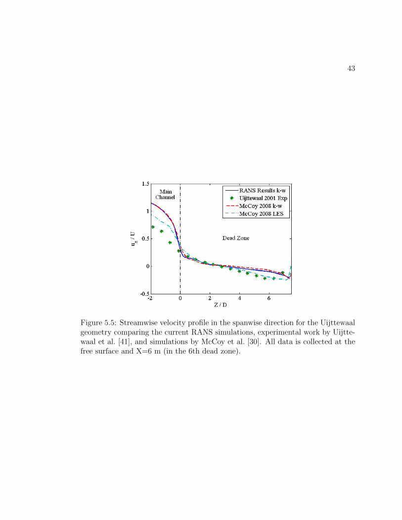
al. [30]. Figures 5.5 and 5.6 show that the current RANS studies are a good match
to the RANS studies done by McCoy. However, there are significant differences
between the RANS and experimental results. McCoy’s LES results match the
experimental results better. The width of the mixing layer is under predicted by
the RANS results and the TKE is over predicted.
43
Figure 5.5: Streamwise velocity profile in the spanwise direction for the Uijttewaalgeometry comparing the current RANS simulations, experimental work by Uijtte-waal et al. [41], and simulations by McCoy et al. [30]. All data is collected at thefree surface and X=6 m (in the 6th dead zone).

44
Figure 5.6: TKE profile in the spanwise direction for the Uijttewaal geometrycomparing the current RANS simulations, experimental work by Uijttewaal etal. [41], and simulations by McCoy et al. [30]. All data is collected at the freesurface and X=6.1 m (in the 6th dead zone).

45
5.4 Series Results
For a regular series of dead zones, it is important to understand how the properties
of the dead zone develop in the series. With enough dead zones in series, it is
expected that the shear layer will eventually become fully developed. That is to
say that the time scales of exchange will become independent of dead zone rank.
Figure 5.7(a) shows how the streamwise velocity varies with streamwise position.
By the fourth dead zone, the velocity profile has become periodic with dead zone
rank. The TKE profile, shown inFigure 5.7(b), is nearly developed by the fourth
dead zone.
Several simulations were also run for the Weitbrecht geometry with variations
in dead zone length and average velocity. Figures 5.9(a), 5.9(b), and 5.9(c) show
the flow patterns in a fully developed dead zone for different dead zone lengths. For
large lengths, the dead zone has one main eddy that is centered slightly downstream
of the dead zone center. There is a secondary eddy in the upstream corner of the
dead zone. The secondary eddy has significantly less momentum than the primary
eddy. As the dead zone length is decreased, the secondary eddy gets smaller and
eventually vanishes around a length equal to 0.65 m. As the length is decreased
further, the main eddy separates into two eddies stacked in the spanwise direction.
Figures 5.8(a) and 5.8(b) show the effect of changes in the average velocity on
the flow distribution. The velocity has little effect on the size or location of the
primary or secondary eddy. The changes in flow structure can be classified based
on the aspect ratio of the dead zone, defined as WL
. For aspect ratios less than one,

46
(a) Streamwise velocity
(b) TKE
Figure 5.7: Flow quantities as a function of streamwise position for the refinedgrid. Data is collected at the free surface on the line that separates the dead zonesfrom the main channel. The developing shear layer is shown for five dead zones.

47
there is a centrally located primary eddy with a secondary eddy possible in the
upstream corner. Large aspect ratios cause multiple eddies to form in a stacked
configuration.
(a) U=0.16 ms (b) U=0.20 m
s
Figure 5.8: Streamlines at the free surface in a dead zone after the shear layer isfully developed for two different average velocities using the Weitbrecht geometry.
(a) L=1.25 m (b) L=0.65 m (c) L=0.25
Figure 5.9: Streamlines at the free surface in a dead zone after the shear layer isfully developed for three different lengths using the Weitbrecht geometry.
A quantitative analysis of the time scales in a dead zone also shows a depen-
dence on the aspect ratio. A useful way to describe the exchange process is by
plotting a ratio of time scales vs. the aspect ratio, a geometric ratio. The time
scales selected are τL and Tconv. These quantities make a ratio of the flushing time
of the dead zone to the time it takes a fluid particle to travel past the dead zone.

48
Figure 5.10 is a plot of the ratio of time scales to the aspect ratio for these RANS
results as well as the experimental results of Weitbrecht et al. [46] and Uijttewaal
et al. [41]. Weitbrecht conducted both particle tracking velocimetry, PTV, and
dye concentration, PCA, studies.
Figure 5.10: Plot of the ratio of the Langmuir to convective time scales vs. theaspect ratio for series of dead zones. Experimental results from Uijttewaal etal. [41] and Weitbrecht et al. [46] are included.
5.5 Single Geometry and Grid
A regular series of dead zones can represent some natural systems well. However,
dead zones in typical streams are usually isolated. For this reason, additional
simulations were conducted on a single dead zone geometry that is a hybrid of the
Weitbrecht and Uijttewaal series geometries. The single dead zone is the cavity

49
type like the Uijttewaal geometry, but has a constant depth like the Weitbrecht
geometry. Figure 5.11 is a plan view of the geometry. Various cases were run for
different widths, lengths, depths, and velocities. Table 5.4 lists the different cases
run. The grid used is shown in Appendix D and has grid spacing smaller than
the refined Uijttewaal series grid. The minimum and maximum grid spacing is in
Appendix D. There are 1.46 million cells in the base case grid.
Figure 5.11: Plan view of the single dead zone geometry. The depth is uniform inthe main channel and dead zone.

50
Table 5.4: Different dead zones parameters used in the single dead zone cases.
Case W [m] L [m] D [m] U [ms ]Base 0.5 1.25 0.046 0.221
2 0.5 1.45 0.046 0.2213 0.5 1.05 0.046 0.2214 0.5 0.85 0.046 0.2215 0.5 0.65 0.046 0.2216 0.5 0.55 0.046 0.2217 0.5 0.45 0.046 0.2218 0.5 1.25 0.046 0.2489 0.5 1.25 0.046 0.19310 0.5 1.25 0.046 0.16511 0.5 1.25 0.046 0.11012 1.25 1.25 0.046 0.22113 1 1.25 0.046 0.22114 0.75 1.25 0.046 0.22115 0.5 1.25 0.092 0.22116 0.5 1.25 0.063 0.22117 0.5 1.25 0.023 0.221
5.6 Single Dead Zone Results
The steady velocity field and transient concentration curve are stored for each of the
cases listed in Table 5.4. The general flow structures are similar to the dead zone
series results. The low aspect ratio cases have a primary eddy with a secondary
eddy in the upstream corner. For aspect ratios around one, the secondary eddy
disappears. The largest aspect ratio studied is 1.1 and does not show the stacked
eddy configuration.
For the series results, Figure 5.10 showed a clear trend when plotting the ratio
of time scales vs. the aspect ratio. The aspect ratio was varied by changing just the

51
dead zone length. Figure 5.12 is a plot of the same time scale ratio. This figure
uses cases that changed the aspect ratio by varying both the length and width
of the dead zone. Both the length and width cases show a nearly linear trend,
but with different slopes. This suggests that the aspect ratio does not entirely
determine the ratio of time scales for a single dead zone.
Figure 5.12: Plot of the ratio of the Langmuir to convective time scales vs. theaspect ratio for single dead zone. Only cases varying L and W are shown.
Section 3.1 details the dimensional analysis of a dead zone system. This analysis
found that a nondimensional quantity, such as the time scale ratio, should depend
on four geometric ratios and one Reynolds number. For these cases, the depth
is constant so hE and hD can be removed. This leaves two geometric ratios and
one Reynolds number. It is also assumed that the time scale ratio will be of the
power law form shown in Equation 5.2. Using four independent cases, a system
of equations can be generated to solve for the four constants, a, b, c, and d. The

52
constants are solved for all the possible combinations of independent cases and then
averaged. Equation 5.3 shows the resulting function. The geometric ratios can be
combined with the Reynolds number and rounded to the nearest whole number.
This gives W 6D4
L9 as an effective length scale of the dead zone. Figure 5.13 shows that
this effective length scale collapses the data for all the cases. The exponents in the
effective length scale determine the importance of each parameter. At this time,
the exact values of these exponents have no physical or analytical explanation.
This correlation can be recast into an expression for the exchange coefficient, k, as
shown in Equation 5.4.
τLTconv
= a(W
L
)b (WD
)c (WU
ν
)d(5.2)
τLTconv
= 156.9(W
L
)1.28 (WD
)−0.56 (WU
ν
)0.14
≈ 157
(W 6D4
L9
U
ν
) 17
(5.3)
k =1
157
(D4
WL2
U
ν
)− 17
(5.4)
In addition to the velocity data, transient passive scalar analyses were run for
each case. Figure 5.14 is a plot of the concentration for the base case after 5000
s. The maximum concentration in the plot is 0.03 as most of the scalar has left
the dead zone. The concentration quickly drops in the circulating region at the
perimeter of the primary eddy. The core region of the primary eddy has slow
moving fluid and low TKE values. This region stays at a high concentration for
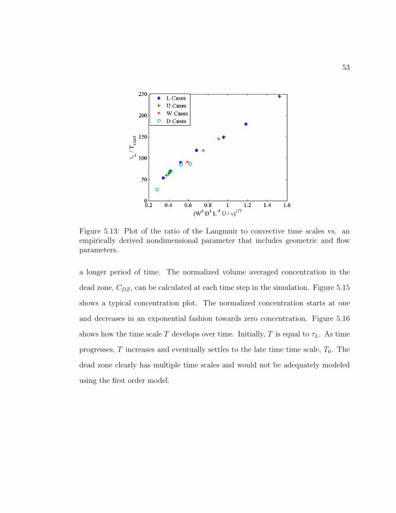
53
Figure 5.13: Plot of the ratio of the Langmuir to convective time scales vs. anempirically derived nondimensional parameter that includes geometric and flowparameters.
a longer period of time. The normalized volume averaged concentration in the
dead zone, CDZ , can be calculated at each time step in the simulation. Figure 5.15
shows a typical concentration plot. The normalized concentration starts at one
and decreases in an exponential fashion towards zero concentration. Figure 5.16
shows how the time scale T develops over time. Initially, T is equal to τL. As time
progresses, T increases and eventually settles to the late time time scale, T0. The
dead zone clearly has multiple time scales and would not be adequately modeled
using the first order model.

54
Figure 5.14: Contour of the concentration within the dead zone for the base singledead zone case. The dark region represents higher concentration.
Figure 5.15: Plot of the normalized dead zone concentration vs. time for the basecase single dead zone geometry.

55
Figure 5.16: Plot of the instantaneous time scale, T , vs. time for the base singledead zone case. τL and T0 are shown for reference.

56
5.7 Two Region Model
Due to finding multiple time scales in the scalar simulation, the single dead zone
results are a good candidate for the two region model. Figure 5.17 shows a plot
of the two region model fit to the base case RANS simulation results. The two
region model fits extremely well throughout the time series. The average percent
error for the base case is 0.71%. Table 5.5 lists the fit parameters τp, τs, and k3
for all the single dead zone cases. The average error for all the cases is 0.64% with
a maximum error of 1.15%. Ideally, the model parameters could also be scaled
Figure 5.17: Plot of the dead zone concentration for the base single dead zonecase. Symbols are from fitting the two region model to the concentration plot.The average error between the two is 0.71%.
based on geometric and flow conditions. However, the model parameters do not
conform to the assumed power law form or many other forms tried. Therefore, the
two region model can only be applied a posteriori to simulated or experimental

57
Table 5.5: Results from fitting the two region model to the single dead zone cases.Model parameters τp, τs, and k3 are shown as well as the average percent error.
Case W [m] L [m] D [m] U [ms ] τp [m] τs [m] k3 % ErrorBase 0.5 1.25 0.046 0.221 457.4 1086.3 0.669 0.71%
2 0.5 1.45 0.046 0.221 372.7 808.5 0.350 0.77%3 0.5 1.05 0.046 0.221 408.0 1148.0 0.637 0.53%4 0.5 0.85 0.046 0.221 410.6 1275.1 0.691 0.82%5 0.5 0.65 0.046 0.221 414.5 1331.9 0.747 1.15%6 0.5 0.55 0.046 0.221 403.3 1115.3 0.745 0.96%7 0.5 0.45 0.046 0.221 347.7 711.4 0.520 0.40%8 0.5 1.25 0.046 0.248 402.1 909.1 0.664 0.74%9 0.5 1.25 0.046 0.193 502.8 1262.1 0.686 0.76%10 0.5 1.25 0.046 0.165 584.4 1449.0 0.645 0.75%11 0.5 1.25 0.046 0.110 593.6 1643.6 0.290 0.60%12 1.25 1.25 0.046 0.221 838.2 4767.9 0.549 0.40%13 1 1.25 0.046 0.221 724.3 4123.8 0.593 0.60%14 0.75 1.25 0.046 0.221 608.0 3284.0 0.674 0.69%15 0.5 1.25 0.092 0.221 69.4 571.0 0.060 0.06%16 0.5 1.25 0.069 0.221 99.0 597.7 0.086 0.22%17 0.5 1.25 0.023 0.221 372.1 1243.4 0.428 0.82%
results.
There are some useful trends that can be taken from the model results. As
the velocity is increased, both τp and τs decrease while the weighting factor k3
stays relatively unchanged. This is somewhat intuitive as increasing the velocities
throughout the system will decrease all time scales. A constant k3 value indicates
that the size and flow properties of the secondary region are somewhat independent
of velocity. This trend is consistent with the qualitative flow structure results from
the series simulations. The width cases also show a clear trend of the time scales
increasing with an increasing width. This is most likely due to increasing the

58
perimeter of the dead zone and thus increasing the time it takes a fluid particle
to circulate around the entire dead zone. k3 tends to decrease with an increasing
width. This trend indicates that the influence of the secondary region is increasing
for larger widths possibly due to increasing the volume of the secondary region
relative to the primary region.
The two region model can also be applied to experimental concentration curves.
Figure 5.18 shows three experimental concentration curves measured by Jackson
et al. [14] in dead zones of small natural streams. The two region model does a
reasonable job of approximating the experimental results with average errors of
14.3%, 12.5%, and 6.29%. Most of the error occurs in the early time. This trend
may be due to slightly different initial conditions. The model assumes the dead
zone is initially at a uniform distribution. The experimental results were obtained
by injecting concentration into the dead zone until a steady condition is reached.
Then injecting is stopped and the concentration curve measured. The steady state
condition could have significant gradients in concentration and would alter the
early time behavior.

59
Figure 5.18: Three experimental concentration plots by Jackson et al. [14] fit withthe two region model.

60
Chapter 6: LES Cases
6.1 Geometry and Grids
The LES cases use a single dead zone version of the geometry used by Uijttewaal.
This geometry has a cavity type dead zone with a non-uniform depth. The single
dead zone is 1.125m long, 0.75 m wide, and has an average velocity of 0.35 ms .
The main channel depth is 0.1 m. The dead zone has an average depth of 0.05 m
and the depth at the dead zone main channel interface is 0.06 m. Figures 5.1(a)
and 5.1(b) show plan view and cross sectional diagrams of this geometry except
this geometry uses only one dead zone.
The LES solver does not use wall models and therefore the grid used must
resolve the boundary layers on both the channel bottom and the side walls. Two
grids were generated to examine what refinement is necessary. Each grid uses
structured hexagonal cells in the dead zone and shear layer. Triangular prism cells
were used in the main channel to reduce the cell count. The grid spacing is highly
stretched near the wall to reduce the cell count, but still resolves the boundary
layer. Table 6.1 shows the grid spacing used for both the coarse and fine grids in
meters and wall units. Appendix E has detailed figures of the grids used. The
coarse grid uses 1.54 million cells compared to the fine grid’s 10.4 million.

61
Table 6.1: Grid spacings for the coarse and refined LES grids in the dead zone andshear layer in meters and wall units.
Coarse GridMin [m] Max [m] Min Max
∆Y 9.24E-5 0.0104 ∆Y + 1.78 200.75∆X 9.24E-5 0.0104 ∆X+ 1.78 200.75∆Z 9.24E-5 0.0129 ∆Z+ 1.78 249.01
Refined GridMin [m] Max [m] Min Max
∆Y 4.62E-5 0.0052 ∆Y + 0.89 200.75∆X 4.62E-5 0.0104 ∆X+ 0.89 200.75∆Z 4.62E-5 0.0064 ∆Z+ 0.89 123.54
6.2 Solution Procedure
The solution procedure for the LES cases is similar to RANS case. First, a fully
developed inlet condition is simulated using a periodic channel and saved. The
actual dead zone geometry is simulated using the inlet condition and the stationary
velocity field is found. The main difference is that LES is a time accurate model
and thus all simulations are transient.
The periodic channel is simulated using a constant mass flow rate condition.
A constant mass flow rate is enforced by adding a uniform body force to the fluid
in the channel. The body force is calculated from a momentum balance of the
channel. Momentum needs to be added through the body force to make up the
difference between the current total momentum and the desired momentum and
to overcome the momentum lost to shear force at the walls. When the periodic
channel has reached a stationary state, the body force will be steady and balance

62
the shear force.
Another important consideration is adding perturbations to the periodic chan-
nel. These perturbations will develop into turbulence. Without adding perturba-
tions, the flow will take a long time to transition to a fully turbulent flow. The
perturbations are added to the initial velocity condition. Sinusoidal perturbations
were added with a magnitude equal to 40% of the average velocity. Linear damp-
ing of the perturbations was used near the wall to ensure the perturbations match
the no-slip condition. The channel was assumed to be fully developed when the
body force term reached a steady state. The fully developed inlet was saved from
a cross sectional plane of the channel at every tenth time step. Data was saved for
a period of time approximately equal to three flow-through times for the actual
geometry.
The saved time resolved inlet condition was used as the inlet boundary con-
dition for the actual dead zone geometry. The inlet data is interpolated in both
time and space to the dead zone grid. When the simulation reaches the end of the
time series of inlet data, it wraps around to the beginning of the inlet data set.
The dead zone simulation is then allowed to run until it has reached a stationary
state, when the time averaged velocities are not changing appreciably. The average
velocity and normal components of the Reynolds Stresses are saved at each time
step. The averaged quantities are then reset and the simulation is allowed to run
until the averages reach steady values. The time step used for the refined grid
is 2.5E-5 seconds. No passive scalar simulations were run with LES due to the
computational expense of running the simulation for 200+ seconds.

63
6.3 LES Results
The average velocity fields for both the coarse and refined grids were stored and
compared to a RANS simulation that uses the same grid as the coarse LES. Fig-
ure 6.1 shows a velocity profile in the spanwise direction. This profile shows that
the coarse and refined LES give similar results. The refined case predicts slightly
lower velocities in the shear region and a more constant slope inside the dead zone.
The RANS velocity profile is significantly different from both LES cases. The shear
layer is smaller and there is zero velocity region near the center of the dead zone.
Figure 6.1: Plot comparing the streamwise velocity profile in the spanwise directionfor both LES grids to a RANS simulation on the coarse grid. The dashed verticalline represents the main channel-dead zone interface. Data is collected at the freesurface and on the X=0.4m line.
The current LES can also be compared to the experimental results by Uijtte-
waal et al. [41] and the LES by McCoy et al. [30]. While Uijttewaal and McCoy

64
use a series instead of a single geometry, the first dead zone should be mostly
unaffected by downstream dead zones. Figure 6.2 shows a velocity profile in the
spanwise direction comparing the two LES simulations with the experimental re-
sults. The current LES case matches the experiments quite well in the dead zone.
The experiments show a lower velocity in the shear layer. There are differences
between the two LES simulations probably due to a more refined grid in this work
or the length of time over which the velocity was averaged.
Figure 6.2: Plot comparing the streamwise velocity profile in the spanwise directionfor this LES study, LES by McCoy et al. [30], and experiments by Uijttewaal etal. [41]. The dashed vertical line represents the main channel-dead zone interface.Data is collected at the free surface and on the X=0.4m line.
Figure 6.3 shows streamlines for the time averaged flow field. The general flow
structure looks similar to the RANS studies shown in Figure 5.9(b) for an aspect
ratio near one. The primary eddy in the LES is slightly more oval. However,
the differences in depth, channel velocity, and series vs. single geometry could
65
contribute to this difference.
The exchange velocity between the dead zone and main channel makes up τL.
Figure 6.4 is a contour plot of the local exchange velocity at the interface between
the dead zone and the main channel. There are distinct regions where the time
averaged flow is into or out of the dead zone. However, the net flow into the
dead zone must be zero to conserve mass. There are strong velocities out of the
dead zone near the stagnation region at the downstream corner. There is also a
large region of flow into the dead zone near the downstream edge and closer to the
bottom of the dead zone. The depth dependence implies that measurements taken
near the free surface may not be representative of the entire flow.
LES provide much more turbulence data than RANS simulations. RANS sim-
ulations treat turbulence as isotropic as the Reynolds Stresses are modeled by the
ratio k and ω, two scalar fields. Figure 6.5 is a contour plot of the u′xu′x component
of the Reynolds Stress tensor. There is a distinct region of increased fluctuations
in the shear layer to turbulent structures shed off the upstream corner of the dead
zone. The largest fluctuations are where the shear layer stagnates near the down-
stream corner. Some of the fluctuations begin to recirculate in the dead zone,
but dissipate quickly. Similar to the RANS simulation, there is a region near the
center of the dead zone with reduced turbulence. However, this region has a more
irregular shape compared to the RANS simulation. Appendix F has additional
plots of the mean velocity and Reynolds Stress.

66
Figure 6.3: Average streamlines at the free surface in the dead zone for the coarse
LES grid.
Figure 6.4: Contours of uzU
, the time averaged exchange velocity at the interface
between the dead zone and main channel for the coarse LES grid. The Y dimension
is stretched by a factor of 10.

67
Figure 6.5: Plan view contours of u′xu′x
U2 at the free surface for the coarse LES grid.
The RANS and LES velocity profiles showed some differences. As a test of
how significant these differences are to scalar transport, a RANS passive scalar
analysis was run using the time averaged flow field from the LES study. No velocity
interpolation was needed as the RANS simulation was also run on the coarse LES
grid. With the LES flow field, the RANS simulation was first allowed to calculated
k and ω. Then a transient passive scalar study was conducted and compared to
an all RANS simulations.
Figure 6.6 shows the time series of both passive scalar studies. The concentra-
tion of the RANS case initially decreases more quickly. At later times, the LES
concentration eventually becomes less than the RANS case. The two region model
was applied to both cases and the resulting parameters are shown in Table 6.2.
Both time scales are significantly smaller for the LES case. The LES k3 value

68
initially puts little weight on τp which explains the slow transport at early time.
At late time when τs dominates, the concentration decreases faster for the LES
case compared to the RANS.
Figure 6.6: Plots of the normalized dead zone concentration vs. time for RANS
scalar studies using the time average flow field from LES and RANS. Both simu-
lations use the coarse LES grid.

69
Table 6.2: Two region parameters, τp, τs, and k3, fit to the concentration plots from
RANS passive scalar analyses using the mean flow field from LES and RANS. The
average percent error between model and simulation is also shown.
τp [s] τs [s] k3 % Error
LES 29.56 493.2 0.156 0.39
RANS 226.9 978.1 0.759 3.54

70
Chapter 7: Conclusions
RANS simulations of series of dead zones were carried out for a range of lengths and
average velocities on similar geometries to past experiments. It was determined
that the flow is fully developed after four dead zones. This result means that only
the first four dead zones need to be studied to get the characteristics of a much
longer series. The time averaged velocity field generally matches the experiment
with a large eddy at the center of the dead zone with additional eddies depending
on the aspect ratio. When τLTconv
is plotted vs. the W/L ratio, the simulations and
experiments show an increasing trend. However, most of this data was generated
using variable dead zone lengths. For the single dead zone geometry, varying both
the width and length showed that τLTconv
depends on more than just the aspect ratio.
This dependence led to additional cases varying the depth and velocity. Nondi-
mensionalizing the results leads to a functional relationship between the relevant
nondimensional groups, WL
, WD
, and ReW , and the time scale ratio, τLTconv
. The
nondimensionalization can be interpreted as a Reynolds number with an effective
length scale of W 6D4
L9 . This length scale was determined empirically and therefore
the exponents have no physical origin. Using this length scale in a Reynolds num-
ber allows τL to be predicted from the easily measurable parameters L, W , D,
and U . If this type of relationship is found to hold good for irregularly shaped
natural dead zones, time intensive tracer experiments would not be needed to get

71
an estimate of τL
The passive scalar simulations showed that the dead zone is not perfectly mixed.
The core of the primary eddy retains scalar longer than the perimeter of the eddy.
This leads to multiple time scales being present in the dead zone. The first order
dead zone model uses a single time scale and is therefore incapable of modeling
these results. A two region model was developed that can be fit to the simulated
concentration plots with minimal error. The model also represents experimental
concentration plots reasonably well despite slightly different initial conditions. The
two region model suggests that the time scales within the dead zone increase with
increasing width and decreasing velocity.
The LES simulations for a single dead zone matched well to experiments and
past LES simulations. The mean velocity distribution in the exchange region shows
a strong dependence on depth. This dependence suggests that measurements taken
near the free surface are not representative of the depth-averaged values. This
limits the effectiveness of surface measurements methods such as tracking floating
particles and highlights the need for full field experimental techniques such as
particle image velocimetry. While the mean velocity profiles are similar between
the RANS and LES studies, there are noticeable differences even for the same
grid. These differences were shown to significantly affect passive scalar studies.
This result diminishes the quantitative predictive capability of the RANS models
for this geometry. However, the trends shown by the RANS simulations serve to
guide future LES and experimental studies into the scaling of the transport time
scales.

72
The results discussed in this work are only valid over the range of nondimen-
sional quantities studied. The ReD values used, 8300-39300, are characteristic of
small natural streams. While the Reynolds number dependence on the flow struc-
tures was shown to be small, rivers likely have different flow features. The aspect
ratio studied are similar to those found in field work by Jackson et al. [14]. Large
aspect ratios where the dead zone flow is almost stagnate and small aspect ratios
where the shear layer could reattach are not considered. There are additional pa-
rameters, such as rough beds, irregularly shaped banks, and high Froude numbers,
that need further experimental and computational work to be incorporated into
existing dead zone models.

73
Bibliography
[1] SV Apte, K. Mahesh, P. Moin, and JC Oefelein. Large-eddy simulation ofswirling particle-laden flows in a coaxial-jet combustor. International Journalof Multiphase Flow, 29(8):1311–1331, 2003.
[2] J.J. Baik, J.J. Kim, and H.J.S. Fernando. A cfd model for simulating urbanflow and dispersion. Journal of Applied Meteorology, 42(11):1636–1648, 2003.
[3] A. Bellucci, G. Buffoni, A. Griffa, and E. Zambianchi. Estimation of residencetimes in semi-enclosed basins with steady flows. Dynamics of atmospheres andoceans, 33(3):201–218, 2001.
[4] K.E. Bencala and RA Walters. Simulation of solute transport in a mountainpool-and-riffle stream with a kinetic mass transfer model for sorption. WaterResources Research, 19(3):732–738, 1983.
[5] B. Biglari et al. Numerical modeling of flow around bridge abutments incompound channel. Journal of Hydraulic Engineering, 124:156, 1998.
[6] K. Chang, G. Constantinescu, and S.O. Park. Analysis of the flow and masstransfer processes for the incompressible flow past an open cavity with a lami-nar and a fully turbulent incoming boundary layer. Journal of Fluid Mechan-ics, 561(4):113–145, 2006.
[7] G. Constantinescu, A. Sukhodolov, and A. McCoy. Mass exchange in a shallowchannel flow with a series of groynes: Les study and comparison with labo-ratory and field experiments. Environmental fluid mechanics, 9(6):587–615,2009.
[8] C. Engelhardt, A. Kruger, A. Sukhodolov, and A. Nicklisch. A study of phy-toplankton spatial distributions, flow structure and characteristics of mixingin a river reach with groynes. Journal of plankton research, 26(11):1351–1366,2004.
[9] M. Germano, U. Piomelli, P. Moin, and W.H. Cabot. A dynamic subgrid-scaleeddy viscosity model. Physics of Fluids A: Fluid Dynamics, 3:1760, 1991.

74
[10] PE Gill, W. Murray, and A. Saunders. Snopt 5.3 user manual. Departmentof Mathematics, University of California, San Diego, 1994.
[11] C. Gualtieri, P.A.L. Jimenez, and J.M. Rodrıguez. Modelling turbulence andsolute transport in a square dead zone.
[12] U. Guide. Star-ccm+ version 4.04. 011, 2009.
[13] C. Hinterberger, J. Frohlich, and W. Rodi. Three-dimensional and depth-averaged large-eddy simulations of some shallow water flows. Journal of Hy-draulic Engineering, 133:857, 2007.
[14] T.R. Jackson, R. Haggerty, S.V. Sourabh, A. Coleman, and K.J. Drost. Themean residence time of lateral surface transient storage zones in streams.Unpublished manuscript, May 2012.
[15] I. Kimura and T. Hosoda. Fundamental properties of flows in open channelswith dead zone. Journal of Hydraulic Engineering, 123:98, 1997.
[16] H.P. Kozerski, R. Schwartz, and T. Hintze. Tracer measurements in groynefields for the quantification of mean hydraulic residence times and of the ex-change with the stream. Acta hydrochimica et hydrobiologica, 34(3):188–200,2006.
[17] M. Kurzke, V. Weitbrecht, and G.H. Jirka. Laboratory concentration mea-surements for determination of mass exchange between groin fields and mainstream. In River Flow, volume 1, pages 369–376, 2002.
[18] I. Langmuir. The velocity of reactions in gases moving through heated vesselsand the effect of convection and diffusion. Journal of the American ChemicalSociety, 30(11):1742–1754, 1908.
[19] L. Larcheveque, P. Sagaut, and O. Labbe. Large-eddy simulation of a subsoniccavity flow including asymmetric three-dimensional effects. Journal of FluidMechanics, 577(1):105–126, 2007.
[20] C. Leibundgut, U. Speidel, and H. Wiesner. Transport processes in riversinvestigated by tracer experiments. IAHS PUBLICATION, pages 211–211,1993.
[21] O. Levenspiel. Chemical Reaction Engineering: An Introduction to the Designof Chemical Reactors. John Wiley & Sons, 1967.
75
[22] K. Lien, JP Monty, MS Chong, and A. Ooi. The entrance length for fullydeveloped turbulent channel flow. In 15th Australasian Fluid Mechanics Con-ference, The University of Sydney, Ausralia, 2004.
[23] DK Lilly. A proposed modification of the germano subgrid-scale closuremethod. Physics of Fluids A: Fluid Dynamics, 4:633, 1992.
[24] J.C. Lin and D. Rockwell. Organized oscillations of initially turbulent flowpast a cavity. Aiaa Journal, 39(6):1139–1151, 2001.
[25] X. Liu and J. Katz. Cavitation phenomena occurring due to interaction ofshear layer vortices with the trailing corner of a two-dimensional open cavity.Physics of fluids, 20(4):41702–41702, 2008.
[26] K. Mahesh, G. Constantinescu, and P. Moin. A numerical method for large-eddy simulation in complex geometries. Journal of Computational Physics,197(1):215–240, 2004.
[27] G.U. Manual. Version 16.0, pointwise. Inc., Fort Worth, TX, 2008.
[28] A. McCoy, G. Constantinescu, and L. Weber. Exchange processes in a channelwith two vertical emerged obstructions. Flow, turbulence and combustion,77(1):97–126, 2006.
[29] A. McCoy, G. Constantinescu, and L. Weber. A numerical investigation ofcoherent structures and mass exchange processes in channel flow with twolateral submerged groynes. Water resources research, 43(5):W05445, 2007.
[30] A. McCoy, G. Constantinescu, L.J. Weber, et al. Numerical investigation offlow hydrodynamics in a channel with a series of groynes. Journal of HydraulicEngineering, 134:157, 2008.
[31] P. Moin and SV Apte. Large-eddy simulation of realistic gas turbine combus-tors. AIAA J. v44, 698, 2006.
[32] E.B. Nauman. Residence time theory. Industrial & Engineering ChemistryResearch, 47(10):3752–3766, 2008.
[33] S. Ouillon and D. Dartus. Three-dimensional computation of flow aroundgroyne. Journal of Hydraulic Engineering, 123(11):962–970, 1997.

76
[34] E. Ozsoy, P. Rambaud, A. Stitou, and ML Riethmuller. Vortex characteris-tics in laminar cavity flow at very low mach number. Experiments in fluids,38(2):133–145, 2005.
[35] R. Rossi and G. Iaccarino. Numerical simulation of scalar dispersion down-stream of a square obstacle using gradient-transport type models. AtmosphericEnvironment, 43(16):2518–2531, 2009.
[36] J.L. Santiago, A. Martilli, and F. Martın. Cfd simulation of airflow overa regular array of cubes. part i: Three-dimensional simulation of the flowand validation with wind-tunnel measurements. Boundary-layer meteorology,122(3):609–634, 2007.
[37] E. Shams and S.V. Apte. Prediction of small-scale cavitation in a high speedflow over an open cavity using large-eddy simulation. Journal of Fluids En-gineering, 132:111301, 2010.
[38] J. Smagorinsky. General circulation experiments with the primitive equations.Monthly weather review, 91(3):99–164, 1963.
[39] Y. Tominaga and T. Stathopoulos. Turbulent schmidt numbers for cfd analysiswith various types of flowfield. Atmospheric Environment, 41(37):8091–8099,2007.
[40] M. Tritthart, M. Liedermann, and H. Habersack. Modelling spatio-temporalflow characteristics in groyne fields. River Research and Applications,25(1):62–81, 2009.
[41] WSJ Uijttewaal, D. Lehmann, and A. Van Mazijk. Exchange processes be-tween a river and its groyne fields: Model experiments. Journal of HydraulicEngineering, 127:928, 2001.
[42] E.M. Valentine and I.R. Wood. Longitudinal dispersion with dead zones.Journal of the Hydraulics Division, 103(9):975–990, 1977.
[43] E.M. Valentine and I.R. Wood. Dispersion in rough rectangular channels.Journal of the Hydraulics Division, 105(12):1537–1553, 1979.
[44] W. Van Balen, WSJ Uijttewaal, and K. Blanckaert. Large-eddy simulation ofa mildly curved open-channel flow. Journal of Fluid Mechanics, 630(1):413–442, 2009.

77
[45] V. Weitbrecht and G.H. Jirka. Flow patterns and exchange processesin dead zones of rivers. In PROCEEDINGS OF THE CONGRESS-INTERNATIONAL ASSOCIATION FOR HYDRAULIC RESEARCH, pages439–445, 2001.
[46] V. Weitbrecht, S.A. Socolofsky, G.H. Jirka, et al. Experiments on mass ex-change between groin fields and main stream in rivers. Journal of HydraulicEngineering, 134:173, 2008.
[47] D.C. Wilcox. Reassessment of the scale-determining equation for advancedturbulence models. AIAA journal, 26(11):1299–1310, 1988.
[48] H. Yao, RK Cooper, and S. Raghunathan. Numerical simulation of incom-pressible laminar flow over three-dimensional rectangular cavities. Journal offluids engineering, 126:919, 2004.
[49] M.F.M. Yossef and H.J. de Vriend. Flow details near river groynes: Experi-mental investigation. Journal of Hydraulic Engineering, 137:504, 2011.

78
APPENDICES

79
Appendix A: k-ω Equations
The turbulent kinetic enery, k, and specific dissipation, ω equations are shown
in Equations A.1 and A.2. The model parameters used are shown in Table A.1.
The k-ω model was selected for its computational efficiency, validation history,
and similarity to past work. This model introduces the two additional transport
equations shown above which adds compuatational expense. However, this model
is significantly less expensive than another popular model, the Reynolds stress
model which adds six equations. The k-ω and k-ε two equation models are widely
used and have been tuned and validated for many different applications including
separated flows similar to a dead zone. Of these two models, the k-ω model was
chosen to match the work done by McCoy et al. [30]. Once this solver was validated
against McCoy’s work, the same model was used for the rest of the studies for
consistency.
uj∂k
∂xj= τij
∂ui∂xj− β∗kω +
∂
∂xj
[(ν + σ∗νT )
∂k
∂xj
](A.1)
uj∂ω
∂xj= α
ω
kτij∂ui∂xj− βω2 +
∂
∂xj
[(ν + σ∗νT )
∂ω
∂xj
](A.2)

80
Table A.1: Table of the model parameters used in the k-ω turbulence model.
Constant Valueα 13
25
β 9125
β∗ 0.09σ∗ 0.5

81
Appendix B: Uijttewaal Grids
Figure B.1: Cross section of the Uijttewaal grid.
Figure B.2: Detailed plan view of the Uijttewaal grid used in a dead zone.

82
Appendix C: Weitbrecht Grids
Figure C.1: Cross section of the Weitbrecht grid.
Figure C.2: Detailed plan view of the Weitbrecht grid used in the dead zone.

83
Appendix D: Single Grid
Table D.1: Table of the grid spacing for the single dead zone geometry in the deadzone and shear layer in both meters and wall units.
Min [m] Max [m] Min Max∆Y 9.24E-05 0.0052 ∆Y + 1.06 59.60∆X 9.24E-05 0.0104 ∆X+ 1.06 119.20∆Z 9.24E-05 0.0104 ∆Z+ 1.06 119.20
Figure D.1: Cross section of the single geometry grid.
Figure D.2: Detailed view of the cross section of the dead zone corner for the singlegeometry grid.

84
Figure D.3: Plan view of the grid used in the single dead zone cases.
Figure D.4: Detailed plan view of the upstream corner of the dead zone for thegrid used in the single dead zone cases.

85
Appendix E: LES Grid
Figure E.1: Cross section of the coarse LES grid.
Figure E.2: Detailed cross section of the dead zone-main channel corner for thecoarse LES grid.

86
Figure E.3: Plan view of the coarse LES grid.
Figure E.4: Detailed plan view of the upstream corner of the dead zone for thecoarse LES grid.

87
Appendix F: Additional LES Plots
Figure F.1: Plan view contours of u′zu′z
U2 at the free surface for the coarse LES grid.
Figure F.2: Plot ofu′yu
′y
U2 at the dead zone-main channel interface for the coarse
LES grid.

88
Figure F.3: Plot of u′zu′z
U2 at the dead zone-main channel interface for the coarse
LES grid.
