Alternative Monetary Policy Rules for India

Michael Debabrata Patra and Muneesh Kapur

WP/12/118

© 2012 International Monetary Fund WP/12/118

IMF Working Paper

Office of Executive Director

Alternative Monetary Policy Rules for India

Prepared by Michael Debabrata Patra and Muneesh Kapur1

Authorized for distribution by Mr. Arvind Virmani

April 2012

Abstract

This paper empirically evaluates the operational performance of the McCallum rule, the Taylor rule and hybrid rules in India over the period 1996–2011 using quarterly data, with a view to analytically informing the conduct of monetary policy. The results show that forward-looking formulations of both rules and their hybrid version - setting a nominal output growth objective for monetary policy with an interest rate instrument - outperform contemporaneous and backward-looking specifications, especially when targeting core components of GDP and inflation, and combine the best parts of efficiency and discretion.

JEL Classification Numbers:E31; E32; E52; E58; F41

Keywords: India, McCallum Rule, Monetary Policy, Monetary Policy Reaction Function, Neutral Interest Rate, Taylor Rule

Author’s E-Mail Address: mpatra@imf.org; mkapur@imf.org

1 The authors are grateful to Masahiko Takeda and Roberto Guimaraes-Filho for useful comments. Secretarial assistance from Suryanarayana Gopavajhala is thankfully acknowledged. The views expressed in the paper are attributable to the authors only and do not necessarily represent those of the institution(s) to which they belong. All other usual disclaimers apply.

This Working Paper should not be reported as representing the views of the IMF. The views expressed in this Working Paper are those of the author(s) and do not necessarily represent those of the IMF or IMF policy. Working Papers describe research in progress by the author(s) and are published to elicit comments and to further debate.

2

Contents Page

I Introduction 3

II. Select Empirical Literature 5

Two Modern Formulations 7

McCallum Rule 9

Taylor Rule 12

III. India’s Monetary Policy Framework 15

IV Methodology, Data and Estimation Results 19

McCallum Rule 22

Hybrid McCallum-Taylor Rule 24

Hybrid McCallum-Hall-Mankiw Rule 26

Taylor Rule 27

Alternative Interest Rate Rules in the Literature 32

V. Summary and Conclusion 35

References 37

Tables

1 Estimates of McCallum Rule 24

2 Estimates of Hybrid Taylor-McCallum Rule 26

3 Estimates of Hybrid McCallum-Hall-Mankiw Rule 27

4 Estimates of Taylor Rule (Forward-looking Specifications) 30

5 Estimates of Taylor Rule (Contemporaneous Specifications) 31

6 Alternative Taylor-type Monetary Policy Rules 33

7 Simulation Results for Alternative Monetary Policy Rules 34

Annex

I List of Variables 43

3

“….do not imagine that any actual central bank would ever turn their determination of instrument settings over to some clerk armed with a simple formula and a hand calculator—or even to a team of PhD economists armed with computers and Matlab simulation programs.”

------Bennett McCallum, 2002

I. Introduction

Should monetary policy be conducted by rules known in advance or by the policy

maker’s discretion? This question, as unsettled today as it was in its origins (Simons, 1936)2,

continues to haunt the ‘how’ of monetary policy conduct. In the slipstream of ‘seminal’ work

in the late 1970s on time–inconsistency, this debate has turned out to be among the most

enduring and prolific in the literature. The case for rules was demonstrated across a general

class of models rather than a specific view of the world such as the celebrated monetary rule

(Friedman, 1960) – discretion implies selecting the decision which is best, given the current

situation, but this may result either in consistent but sub-optimal planning or in economic

instability (Kydland and Prescott, 1977).

Practitioners have argued that this advocacy for rules tends to trivialize one of their

important concerns: how to account for the uncertainty in the link between policy

instruments and ultimate objectives (Carlson, 1988). This warrants some flexibility,

especially in the face of unforeseen contingencies that are potentially destabilizing and

accordingly, it is reasonable to adopt a more pragmatic approach of rules with discretion.

While the dialectic continues to evolve, it is generally recognized that discretion is essentially

related to some sense of an underlying rule or deviation therefrom. The dichotomy between

rules and discretion has to be seen as a continuum, and the actual practice of monetary policy

as a point in this continuum determined by the degree of predictability of the relationship

between goals and instruments. In fact, if predictability exists or at least variability is

systematic, it is possible to incorporate feedback into a rule. Accordingly, using economic

theory to evaluate alternative policy rules that are easily operated and understood is a valid

exercise to inform policy making.

2 Henry Simons discussed the issue as a choice between rules and authorities. In his view, “definite, stable, legislative rules of the game as to money are of paramount importance to the survival of a system based on the freedom of enterprise.” 

4

Operating characteristics are important as they determine the degree of commitment

of the monetary authority to the rule. If commitment is low and therefore discretion is high, it

generally reflects difficulties in making the rule operational. Thus, operationalising a policy

rule and evaluating its performance over time assumes importance. In this context, two

proposals – McCallum (1987) and Taylor (1993) - have raised the debate to an operationally

concrete level. Both recognize the need for flexibility but differ in the manner in which

flexibility is incorporated into the rule. By attempting to reduce uncertainty, both try to

secure the credibility of monetary policy and to avoid the inefficiencies of time inconsistency

associated with pure discretion. Empirical checks of their operational characteristics have

naturally fascinated economists. In the recent period, a welcome development has been the

growing strand of work on empirically testing for the operability of these alternative policy

rules for emerging economies (Koivu, Mehrotra and Nuutilainen, 2008; Mehrotra and

Sanchez-Fung, 2011; Khakimov, Erdogan and Uslu, 2009; Sun, Gan and Hu, 2010) and

particularly for India (Virmani, 2004; Patra and Kapur, 2012). These efforts reflect a

recognition of improvements in institutional frameworks of monetary policy regimes in these

countries that has enhanced the operational autonomy of monetary authorities, alongside the

growing sophistication of financial markets.

This paper joins the growing literature on this strand of work by empirically

evaluating the operational performance of the McCallum rule and the Taylor rule in India,

recognising that such an exercise has to be country-specific. The exercise spans the period

1996-2011 which witnessed two different policy regimes and the transition from one to the

other. Consequently, the findings of the paper are able to throw some light not only on the

operational feasibility of each rule in the Indian context but also on the degree of

commitment of policy authorities to rules and variations therein, if any. Section II explores

the literature on empirical features of the two alternative policy rules with a view to teasing

out nuances and caveats that will condition the estimation and evaluation of the rules in the

Indian context. Section III profiles the historical development of monetary policy conditions

in India over the period of study against the backdrop of macroeconomic and financial

developments that were the setting for prevailing policy regimes and shifts. This provides a

reality check for the choice of alternative policy rules. Section IV describes the estimation

framework, results and salient inferences. Section V offers some concluding remarks.

5

II. Select Empirical Literature

Over the recent decades, there has been a silent revolution. Modern central banks and

monetary authorities have increasingly shed secrecy and mystique to engage in

communicating to the public their policy framework and rationale, their goals and why they

chose them, and the manner in which they intend to achieve their stated objectives. They and

the public have shown a preference for a monetary policy that is disciplined by principles of

systematic conduct so that the temptation of higher inflation can be resisted, accountability

and credibility can be earned, and policy uncertainty among market participants reduced.

This reveals a conscious effort to mitigate the problem of dynamic inconsistency extensively

studied in the literature, with proximate solutions ranging from reputation-building (Barro

and Gordon, 1983), choosing a conservative central banker (Rogoff, 1985), optimal contracts

for central bankers (Walsh, 1995) to some kind of pre-commitment to a policy rule.

In this context, it is useful to start with some home truths. One monetary policy rule is

better than another only if it results in better economic performance according to some

criteria such as inflation or the variability of inflation and output. Neither theory nor evidence

points convincingly to any of the numerous competing models as superior in explaining the

interaction of nominal and real variables as occurs in actual practice. The relevance of

expectations of the future and events of the past to current decisions gives the modern-day

rules a dynamic feature. Shocks to preferences or technology or simply to decision rules

make them stochastic. The rules pertain to the whole economy, not to an individual sector,

and this makes them general equilibrium rules. Each of them incorporates some kind of

temporary nominal rigidity, usually a variant of staggered wage or price setting, which

results in a short-run trade-off between inflation and output or unemployment. With

stochastic shocks, the trade-off is characterized as one between the variance of inflation and

the variance of output, but there is no long-run trade-off.

Simple policy rules work well; their performance is surprisingly close to that of fully

operational policies and more robust than complex rules across a variety of models. Although

policy rules can be written down algebraically, they will probably be more useful as

guidelines than as mechanical formulae for policy makers to follow exactly at least for the

near future (Taylor, 1999a). A good rule is, therefore, one that provides a useful starting

point for central bank deliberations. A central bank can benefit from having a collection of

6

alternative good rules – rules that have optimal properties in a variety of models. This helps

to deal with the uncertainty inherent in the monetary policy process – model uncertainty

emanating from a variety of assumptions, and situation uncertainty – uncertainty about the

current state of the economy and about where the economy would be going with no change in

the policy rate (Feldstein, 1999).

A Brief Historical Journey

The quest for monetary policy rules has been traced back to the writings of Wicksell3

who argued that the central bank should aim to maintain price stability. This simple interest

rate rule did not attract much attention in policy discussions, perhaps because its exclusive

focus on price stability and lack of explicit reference to developments in real economic

activity did not go down well with the ruling orthodoxy of the day.

An early influential case for rules is reflected in the Chicago view which produced

non-activist formulations (Friedman, 1960; Lucas, 1980). A simple but operable policy rule

developed and revolutionized thinking on monetary policy in its time and beyond - that the

central bank maintain a constant rate of growth of the money supply equivalent to the rate of

growth of real GDP or the celebrated k-percent rule4. Giving governments any flexibility in

setting money growth was believed to lead to inflation; countercyclical Keynesian-type

monetary policy was to be avoided at all costs. During the 1960s and 1970s, Friedman’s

recommendation was that the Federal Reserve control the rate of money supply growth at 4

percent. The advantage of the constant money growth was that very little information was

required to implement it. If velocity does not exhibit a secular trend, the only required

3 “If prices rise, the rate of interest is to be raised; and if prices fall, the rate of interest is to be lowered; and the rate of interest is henceforth to be maintained at its new level until a further movement in prices calls for a further change in one direction or the other." (Wicksell, 1898; 1936). See Woodford (2003) and Orphanides (2007) for a brief account of this historical retrospective. 4 "The stock of money [should be] increased at a fixed rate year-in and year-out without any variation in the rate of increase to meet cyclical needs" (Friedman 1960). “A set of aggregative policies which would I believe, lead, and have led, to satisfactory general economic performance are, compactly described: 1. A 4% annual rate of growth of M1, maintained as closely as possible on a quarter-to-quarter basis. 2. A pattern of real government expenditures and transfer payments, varying secularly but not in response to cyclical changes in economic activity 3. A pattern of tax rates, also varying secularly but not in response to cyclical changes in economic activity, set to balance the federal budget on average. 4. A clearly announced policy that wage and price agreements privately arrived at will not trigger governmental reactions of any kind (aside from standard antitrust policies and the general policy of government preference for low over high bids). The first three of these policy rules are taken directly from Friedman’s writing. The fourth is simply a recognition of the fact that, since the time Friedman’s proposals were originally formulated, intervention in the details of private price and wage negotiations has ceased to be viewed as an emergency measure so that a position on the generally accepted aspects of aggregative policy cannot omit mention of this fact.”(Lucas, 1980)

7

element for calibrating the rule is the economy's natural growth of output. In addition, the

calibration of this rule does not rest on the specification of any particular model and is stable

across alternative models of the economy. Despite its intuitive appeal, however, the

Friedman rule became difficult to operate in the face of real world developments as is well

known. High inflation and a breakdown in the stability of the velocity of money brought on

by deregulation of financial markets, innovations and advances in transactions technology

made control of money supply futile. It suffered from logical weaknesses too. Ruling out

policy feedback implied a belief that money was the exclusive determinant of GDP.

Moreover, if a particular money rule would stabilize the economy, discretion preferring

policy makers could always behave that way and still retain the flexibility to change the rule

as needed (Fischer, 1988).

Two Modern Formulations

The McCallum and Taylor rules are essentially efforts to develop simple and

transparent rules that could deliver improved macroeconomic performance. They belong in

the suite of rules driven by the belief that central banks should respond to evolving

conditions in a relatively activist manner, in contrast to the types of rules proposed by the

Chicago school.

The McCallum rule (McCallum, 2000) specifies the growth rate of the monetary base

(instrument) in a non-discretionary feedback rule for nominal GDP (target) as

Δbt = Δx* − Δvt + 0.5(Δx* − Δxt-1),

where Δbt is the rate of growth of the monetary base; Δvt is the rate of growth of base

velocity averaged over previous four years5; Δxt is the rate of growth of nominal GDP and

Δx* is the target rate of growth of nominal GDP (assumed at 5 percent by McCallum for the

US) taken to be the sum of π*, the target inflation rate (2 percent), and the long-run average

rate of growth of real GDP (3 percent per year). Since technological and regulatory changes

5 In a quarterly model, ∆vt = average growth of the base velocity over the previous 16 quarters = (1/16)*[(xt-1 – bt-1 ) – (xt-17 – bt-17)]. Growth rate variables such as Δxt have been measured as changes in logs. Therefore, such variables reflect quarterly changes, not annulized, and in fractional (rather than percentage) units. Accordingly, such variables need to be multiplied by 400 to be commensurate with similar variables as measured by Taylor and in most papers concerned with policy rules (McCallum, 2000).  

8

alter the growth of base velocity from year to year, a problem that undermined Friedman’s

rule, Δvt is averaged over the past four years and is intended as a forecast of the average

growth rate of velocity over the foreseeable future rather than a reflection of current cyclical

conditions which are represented by the term Δx* − Δxt-1. In substance, base money growth

must equal the targeted growth of nominal GDP. There is a proportional feedback to the

growth rate of base money from the gap between nominal GDP growth and its targeted rate.

If the relationship between the monetary base and nominal income changes (say on account

of financial innovations), the growth rate of the monetary base must be adjusted accordingly.

The Taylor rule (Taylor, 1993) prescribes the adjustment of interest rate policy

instrument in a systematic manner in response to developments in inflation and

macroeconomic activity. It can be written as

Rt = r + Δpt + 0.5(Δpt − π*) + 0.5 ýt

where Rt is the nominal policy interest rate; r is the average equilibrium real interest

rate; Δpt is the inflation rate, recent or expected future value; π* is the target rate of inflation,

and ýt is the deviation of current real GDP from its potential or natural rate.

Taylor has used 2 percent for the average real rate of interest and has also assumed

that 2 percent per year is the target rate of inflation. Different values could be specified for

the coefficients on the terms (Δpt − π*) and yt, but the values of 0.5 were used in Taylor’s

original work. The presence of the term Δpt on the right hand side implies that a measure of

the real rate of interest, Rt − Δpt, is adjusted up or down relative to the average real rate r in

response to departures of inflation and output from their target values. Taylor also noted that

if the deviation of real quarterly output from a linear trend is used to measure the output gap,

and the year-over-year rate of change of the output deflator to measure inflation, this

parameterization appeared to describe Federal Reserve behavior well in the late 1980s and

early 1990s.

9

Methodological Issues

In essence, a rule is a restriction on the monetary authority’s discretion. Most rules

proposed in the literature do not, however, eliminate discretion completely6. Modern policy

rules recognize the desirability of some discretion in the monetary authority’s response to the

evolving state of the economy, and, therefore, incorporate feedback that allow it to react in a

manner that minimizes the persistence of shocks. Both the McCallum rule and the Taylor

rule incorporate feedback. While some evidence suggests improved performance, responding

to the state of the economy can also be destabilizing. It is also important to take note of the

Lucas (1975) critique and carefully consider the implications of changes in policies for

expectations – what expectations of prior policy are built into the model and how the model

will change with a new policy.

Methodological issues surrounding the operationalisation of rules essentially relate to

the manner in which feedback is incorporated – the choice of policy instrument that the

monetary authority can control directly and/or accurately – base money for McCallum and

the short-term policy rate for Taylor (in some cases, the exchange rate); the target variable(s)

– deviation of nominal GDP growth from its target for McCallum and deviations of

inflation/real output from target/potential for Taylor (variants also incorporate the exchange

rate); the baseline for the target variable – long run rate of nominal output growth for

McCallum and the real rate of interest for Taylor; the monetary policy response parameter –

the coefficients on the target variables; and the smoothing parameter (the coefficient on the

lagged policy variable) which empirical analysis has shown to be important in gauging the

pace of policy response.

(a) McCallum Rule

Turning to specific methodological issues, first, it is important to note that the policy

instrument in the McCallum’s rule i.e., the monetary base implicitly sums the effects of pure

changes in high-powered money and those induced by changes in reserve requirements.

Given the tendency of the central bank to systematically offset changes in reserve

6 Even a relatively inflexible Friedman-type rule that prescribes a constant rate of money supply irrespective of developments in the economy can allow substantial judgment about the choice of instrument or of timing.

10

requirements with open market operations, the explanatory power of the monetary base as a

policy instrument is significantly improved by adjusting for the short-run dynamics

embodied in discrete changes in reserve requirements (McCallum, 1990; Haslag and Hein,

1995).

Second, the McCallum rule employs average velocity growth because trends in

velocity growth can shift over time, but not every change in base velocity represents a long-

lasting shift in the trend (McCallum and Nelson, 1999). The velocity growth adjustment is

intended to reflect long-lasting institutional/technological changes affecting the demand for

the monetary base7.

Third, the term for deviations of nominal GDP growth from target is intended to

account for cyclical influences and acts as an error-correction mechanism. As in all error-

correction models, this confronts a trade-off between gradualism and immediate restoration

of the target. Thus, the key element in McCallum’s rule is the monetary response coefficient

which determines how much base money – and eventually money stock – must change when

nominal GDP deviates from its target. If the monetary response factor is too large, it can

induce an explosive reaction or instability in the economy. On the other hand, a monetary

response factor that is too small implies that monetary policy does not affect the economy

much. There seems to be a range of ideal values for the monetary response factor (Croushore

and Stark, 1996). McCallum’s own research and other efforts (Hall, 1990) suggests using a

factor of 0.5 for the US economy. In contrast, a lower feedback value (0.25) is needed for

Japan (McCallum, 1993). For developing countries such as China, a smaller monetary

response factor is found to be appropriate (Sun et al, 2010). Clearly, instrument instability is

an important issue that has to be dealt with in a country-specific manner in the context of

estimating McCallum’s rule.

Fourth, McCallum rule also features feedback adjustments in velocity changes in

response to cyclical departures of nominal income from the target path with the coefficient

chosen to balance against the danger of instrument instability. However, the velocity

7 Dueker (1993) uses a time-varying coefficient model with heteroscedastic errors, claiming the advantage of forecasting information about a host of explanatory variables besides the dependent variable, and better adaptation to structural breaks. 

11

correction term could be omitted without any appreciable effect on results, attesting to the

non-dependence of the McCallum rule on base velocity growth (McCallum, 2002).

In empirical analysis McCallum showed that if a rule such as his had been followed,

the performance of the U.S. economy likely would have been considerably better than actual

performance, especially during the 1930s and 1970s, the two periods of the worst monetary

policy mistakes in the history of the Federal Reserve (McCallum, 2002). Several studies

present supportive evidence for McCallum’s rule in different developed countries (Hall,

1990; Judd and Motley, 1991; 1993; Razzak, 2003; Diez de los Rios, 2009). In the Indian

context, a backward-looking version of McCallum’s rule, with real exchange rate changes as

an additional variable, has been found to work best. The nominal income gap is significant

and correctly signed, suggesting that nominal income could be an implicit final target in the

conduct of monetary policy (Virmani, 2004). The McCallum rule has been evaluated along

with Taylor-type and hybrid rules for Russia with the finding that monetary aggregates can

indeed be used as an effective policy instrument (Esanov et al, 2004). In the Chinese context,

the monetary base has been substituted with broad money first by using the coefficients

specified by McCallum, and then by allowing the data to determine the actual coefficient

estimates. The actual developments of the monetary base were found to follow the values

implied by the McCallum rule more closely than was the case with broad money since 2003.

Monetary growth was observed to have been faster than what the McCallum would have

suggested in the more recent period, partly due to hikes in reserve requirements boosting the

monetary base (Koivu et al, 2009). For Turkey, the monetary response coefficient was found

to be 0.1 (as against McCallum’s original proposition of 0.5) in view of the history of high

inflation. Monetary policy appears to be closely simulated by McCallum’s rule over the

whole period (2002-2008) whereas the Taylor rule provides a good approximation only from

2006 when prerequisites of an inflation targeting regime were in place. The smoothing

component was also found to be higher under the McCallum rule (Khakimov et al, 2009).

Drawing on the results of estimating McCallum and Taylor rules as well as hybrids

mixing instruments and targets for 20 emerging countries across Africa, Asia, emerging

Europe and Latin America, it is observed that while the McCallum rule works well for

countries that adopt leaning against the wind strategies, it is the hybrid McCallum-Taylor

specifications with an interest rate instrument and a nominal income gap perform better than

12

benchmark Taylor or McCallum rules. Instrument smoothing is significant across all

specifications, but the exchange rate is not consistently significant (Mehrotra et al, 2011).

(b) Taylor Rule

The confluence of the econometric evaluation evidence and its usefulness for

understanding historical monetary policy has generated widespread interest in the Taylor rule

among numerous central banks to provide guidance in policy decisions. A generalized Taylor

rule that nests the original specification and also allows for interest rate smoothing has been

favoured in the empirical literature (Clarida, Gali and Gertler, 1998, 2000).

A key issue in the context of estimating the Taylor rule is, first, the size of the

coefficients on the inflation and output gaps. The coefficient on inflation is 1.5, the

coefficient on real output is 0.5 and the intercept term is r – 0.5 π* (Taylor, 1993, 1999a).

Some studies have shown that that the coefficient on real output is close to 1 (Brayton et al,

1997). However, higher weight to output in a policy rule gives a lower variance of output but

may give a higher variance of inflation. Raising the coefficient on real output from 0.5 to 1.0

represents a trade-off between inflation variance and output variance, but the increase in

average inflation variability is small compared with the decrease in average output

variability, and moreover, interest rate variance is higher (Taylor, 1999b)

There is less ambiguity around the coefficient on the inflation gap. If the coefficient

on inflation is less than one, the real interest rate would fall rather than rise when inflation

rose (US in 1960s and 1970s), leading to even higher inflation and inflation would turn

highly volatile. There can be bursts of inflation and output fluctuations that result from self-

fulfilling changes in expectations (Clarida et al, 1998).

Second, methodological issue relating to operationalising the Taylor rule is about

whether it should be forward-looking, contemporaneous or backward-looking. While Clarida

et al (1998) demonstrate the case for a purely forward-looking rule in the context of the US,

the UK and Japan, it is also argued that a rule that uses only information about the recent

behavior of inflation and output does quite well (Taylor and Williams, 2010), as compared to

one that uses forecasts of future inflation and output. Performance under the best kind of rule

of this kind (measured in terms of variability of inflation, output and interest rates) is not

significantly reduced if lagged inflation data is used (Rotemberg and Woodford, 1999;

13

Feldstein, 1999). Thus lags in the availability of accurate measurement of inflation are not

necessarily a serious problem for the implementation of such a rule. Accordingly, backward

looking rules are quite good approximations of optimal policy (Rotemberg and Woodford, op

cit.). It is argued that there is no need for policy to be forward-looking as long as the private

sector is. A commitment to raise interest rates later, after inflation increases, is sufficient to

cause an immediate contraction of aggregate demand in response to a shock that is expected

to give rise to inflationary pressures – aggregate demand depends on future interest rates and

not simply on current short rates as long as the monetary authority is understood to be

committed to adhering to the contemplated policy rule in the future and not only at the

present time; and as long as the private sector has model-consistent rational expectations.

However, for the euro area, there is evidence that policy-makers are neither purely backward

nor forward-looking, but react to a synthesis of the available information on the current and

future state of the economy (Blattner and Margaritov, 2010).

Third, adding the exchange rate - either though a monetary conditions index

(weighted average of exchange rate and inflation rate) to replace the interest rate as the

policy instrument or by introducing an exchange rate term in the right hand side - to the

simple Taylor-type policy rules may improve macroeconomic performance (Ball, 1999).

Mohanty and Klau (2004) estimated an open economy Taylor rule for India, along

with other emerging market economies (EMEs) in which the relationship between the short-

term interest rate and the inflation rate turned out to be relatively weak, whereas the output

gap was statistically significant. Similar findings are reported in other efforts (Inoue and

Hamori, 2009; Singh, 2006; Jha, 2008; Hutchison et al, 2010; and Anand et al, 2010). On the

other hand, a comprehensive analysis of monetary policy rules across different specifications

in both backward- and forward-looking versions found monetary policy’s reaction to

inflation to be stronger than to the output gap for the period 1988-2009 (Singh, 2010). On the

basis of a variety of alternative simulations, a forward-looking Taylor rule performed best for

India in term of consistency with the Taylor principle. The coefficient on the inflation gap

turned out to be greater than unity, while that on the output gap was unity (Patra and Kapur,

2012).

Methodological issues that arise in the actual estimation of the Taylor rule and its

extensions have been comprehensively surveyed recently (Patra and Kapur, 2012). First, it is

14

observed that while a forward-looking specification is recommended in theory (the target

variables depend not only on the current policy stance but also on expectations about future

policy), from practical considerations, a general specification with forward-looking terms and

incorporating the well-documented interest rate smoothing by central banks (inertia in policy

response) is preferred in the empirical literature (Clarida et al., 2000; Paez-Farrell, 2009).

Second, exchange rate smoothing is found to be an important consideration in the policy

reaction function of emerging economies, including India, in some studies.8 Third, the use of

the output gap, a variable which is not observed, presents a challenge particularly in view of

frequent and often sizable revisions which can produce large divergences between real time

data on which authorities make their policy judgments and the final revised data that are used

in empirical work. Accordingly, it may be optimal to replace the output gap variable with its

first difference (Taylor and Williams, 2010).

The greater prominence of the Taylor rule is attributed to it being more realistic in

describing the conduct of actual monetary policy since 1986. Modern central banks focus

upon interest rates, not the monetary base, in designing their policy actions. The ascendency

of the new Keynesian framework from the late 1990s has also implied a downgrading of

monetary aggregates in explaining the operational conduct of monetary policy. These

developments notwithstanding, considerable academic support for nominal spending targets

has existed since 1980 (Meade, 1978; Tobin, 1980). Keeping nominal GDP close to a target

growth path would maintain inflation close to its desired value on average and would

diminish fluctuations in real cyclical aggregates. This helps the policy maker to balance the

two goals without having to control or accurately predict how nominal GDP divides between

its constituents (McCallum, 1988). It also eliminates policy surprises due to undesirable

fluctuations arising from pursuit of an optimal policy decision. Also, there is an observable

tendency for an interest rate instrument to become something of a target variable that is thus

adjusted too infrequently and too timidly (Taylor, 1999b).

In some ways, nominal income targeting rules can claim analytical superiority over

pure interest rate formulations in the Taylor rule tradition. Illustratively, the growth rate

version of nominal income targeting avoids the need to measure unobservables such as

8 See also Mohanty and Klau, 2004 for a review.

15

capacity or natural-rate output (for the output gap) or the real interest rate, as is required by

Taylor’s rule9 (Orphanides, 2003). While Clarida et al (1998) provided formal econometric

support for Taylor’s findings in the context of US monetary policy, it has been shown that

replacing expected future inflation in Clarida et al by expected current nominal income

growth produces standard errors that are lower, and nominal income growth is significant

with higher explanatory power (McCallum, 2000). Especially in an environment with near-

zero short-term interest rates, the McCallum rule may be of interest – (Goodfriend, 2000;

Krugman, 1998; Meltzer, 1998). Moreover, in the case of emerging economies, it has been

claimed that a monetary base or some other monetary aggregate can still be a reasonable

monetary policy instrument (Taylor, 2000; Beck and Wieland, 2008).

Experiments with hybrid rules have yielded promising results. Replacing the

monetary base in the McCallum rule with the interest rate as the policy instrument produces a

modified rule that is highly cointegrated with the standard Taylor rule. With similar degrees

of sufficiently high instrument smoothing, each of these rules performs as well as the other –

equality of unconditional variance of inflation and output cannot be rejected (Razzak, 2003).

This seems to be the desirable direction of future research – a consensus approach.

III. India’s Monetary Policy Framework

Proper judgment is important in selecting which reaction function is adequate on the

basis of the declared policy regime and the institutional idiosyncrasies. The selected

empirical rule would then be robust to minor variations (Mehrotra et al, 2011). Accordingly,

before proceeding with the actual estimation of alternative policy rules for India and

evaluating their performance, it is useful to undertake a brief review of the institutional and

operating framework of monetary policy in India so as to situate the choice of policy rule in

an appropriate perspective. In this context, Patra and Kapur (2012) provides a panoramic

9 As pointed out in McCallum (2000), reliance of a policy rule upon any output gap measure is risky, for different measures give different values. Linear de-trending depends rather sensitively on the time period selected for fitting the trend. With respect to the HP filter, the problem is that this procedure produces a trend that is so flexible that it follows the path of actual GDP rather closely, yielding measures of the output gap that would appear to underestimate the economically relevant gap values. McCallum and Nelson (1999) argue that any gap measure based on an output de-trending procedure is conceptually inappropriate – positive shocks serve to increase the value of capacity output, not the values of output relative to capacity.  

16

account of the history of monetary policy regime changes in India - the period up to the mid-

1980s when monetary policy was dominated by fiscal policy did not matter, followed by

monetary targeting with feedback, and then again in the late 1990s when interest rates

progressively became the main instrument of monetary policy.

Up to the early 1980s, the conduct of monetary policy was reduced to a passive

accommodation of budget deficits. The second round effects of such monetization had

serious inflationary consequences that had to be tackled by curbing credit to the private

sector. Apart from recourse to reserve requirements acting as statutory preemptions,10

sectoral credit allocations were put in place, while panoply of interest rates were

administered.

It was in this milieu that a wholesale rethinking of the manner in which monetary

policy is to be conducted was set in motion11. From the second half of the 1980s, elements of

a new regime were gradually put in place. While sub-serving the broader goals of overall

economic policy, monetary policy came to be regarded as best suited to achieve price

stability – it is price stability which provides the appropriate environment under which

growth and social justice can be achieved ….money also matters (Rangarajan, 1988).

Empirical estimations of the tolerable or threshold inflation led to the establishment of

inflation in the range of 5-7 percent (but tending to 5-6 percent) as the objective of monetary

policy (Rangarajan, 1997). These estimates are corroborated by recent studies (Mohanty et

al., 2011; Pattanaik and Nadhanael, 2011) Statistical evidence of reasonable stability in the

demand for money yielded the income elasticity of money demand of 1.77 as a key operating

parameter, with the coefficient on inflation at unity (Rangarajan, 1994). The policy rule came

to be formulated in the form of monetary targeting with feedback. Broad money (M3)

became the appropriate intermediate monetary aggregate for which the rule could be set in 10 By 1990, the statutory liquidity ratio had touched 38.5 percent of deposit liabilities. Since increasing the SLR was not adequate, the Reserve Bank of India become a residual subscriber to the government borrowing programme. In order to curb the expansionary impact of reserve money, the cash reserve ratio had to be progressively increased to 15 percent by 1990 (Rangarajan, 2001).

11 In order to provide a robust analytical framework to policy, a committee was appointed under the chairmanship of Sukhamoy Chakravarty. Dr. Chakravarti Rangarajan, then deputy Governor of the RBI was an important member. The committee recognized the existence of a multiplicity of objectives of monetary policy in India, but assigned eminence to price stability. The committee also recommended monetary targeting, coordination between the government and the central bank on the extent of monetization, and a basis for the determination of the interest rate structure that would ensure positive real interest rates and allow greater freedom to banks in setting lending rates.

17

growth rate range formulation. The money multiplier had been found to be stable and

predictable (Rangarajan and Singh, 1984); so the money supply rule in its reduced from

consisted of determining the growth of reserve money adjusted for reserve requirements as

the monetary authority could determine or at least influence the monetary base even in the

presence of fiscal dominance and administered interest rates (Rangarajan, 1985). Ending

automatic monetization of fiscal deficits was addressed in the context of central bank

autonomy (Rangarajan, 1993)12, and over the period 1994-97 it was phased out. In the second

half of the 1980s, various segments of the financial market spectrum were developed; in

particular, within the limits of an administered structure of interest rates, there was a move

towards creating an active money market which could serve as a transmission channel for

monetary policy (Rangarajan, 2001). Between 1988 and 1997, interest rates were rationalized

and allowed to be freely determined in the market. This coincided with the institution of

financial sector reforms from 1992-93, a market-determined exchange rate, current account

convertibility and a progressive liberalization of the capital account.

The institution of the regime employing interest rates as the main instrument of

monetary policy transmission can be located in 1997 when the Bank Rate was reactivated

after a hiatus of seven years in an environment of development and deepening of various

segments of the financial markets, and the progressive deregulation of interest rates. The

analytics underpinning the monetary policy framework also underwent a silent

transformation in the later part of the 1990s. In its monetary policy statement of April 1998,

the RBI announced that it would switch to a multiple indicator approach “to widen the range

of variables that could be taken into account for monetary policy purposes rather than rely

solely on a single instrument variable such as growth in broad money (M3)”(RBI, 1998). The

era of monetary targeting was drawing to a close and the paradigm in Indian monetary policy

was shifting. In 1999-2000, the stance of monetary policy was conveyed through reductions

in the (reverse) repo rate and the Bank Rate, and India was on the path to a new monetary

policy framework. The reverse repo rates soon began to provide a floor for the overnight call

money market rates while repo auctions were employed in the event of tightness in liquidity

12 “The freedom of the central bank to pursue monetary policy according to its judgment requires that direct funding by the central government is restricted and the limits are made explicit. Then the onus of responsibility of conduct of monetary policy will be squarely on the shoulders of the Reserve Bank where it should logically rest” (Rangarajan, 1993).

18

conditions. It was the Bank Rate, to which all other rates on accommodations by the RBI

were linked, that remained, till 2002, the main signaling rate for conveying the stance of

policy, and the effective ceiling for money market rates.

An Interim Liquidity Adjustment Facility (ILAF) operated through repos and lending

against collateral of Government of India securities was introduced in April 1999. The ILAF

was a mechanism by which liquidity was injected at various interest rates, but absorbed at the

fixed repo rate. Beginning in the following year, a full-fledged LAF was put in place in

stages, providing a reasonable corridor for market play. The Bank Rate progressively gave

way to the repo rate as the upper bound of the policy interest rate corridor. From November

2004, the LAF began to be operated with only overnight repo/reverse repo auctions and

longer-term auctions were discontinued, although the RBI retained the option to conduct

them at its judgment. With the establishment of real time gross settlement, a screen-based

dealing platform and a clearing corporation, intra-day LAF auctions have also been

employed with reasonable success. Over the ensuing period, the LAF has evolved into the

principal operating procedure of monetary policy.

The operating policy rate alternated between repo and reverse repo rates from 2003

till early May 2011, depending upon the macroeconomic and liquidity conditions. There was

the lack of a single policy rate. Against this background, the operating framework was

modified effective May 3, 2011. First, the repo rate was made the only independently varying

policy rate to transmit policy signals more transparently. Second, a new Marginal Standing

Facility (MSF) was instituted under which scheduled commercial banks (SCBs) can borrow

overnight at their discretion up to one per cent of their respective NDTL at 100 basis points

above the repo rate to provide a safety valve against unanticipated liquidity shocks. Third, the

revised corridor was defined with a fixed width of 200 basis points. The repo rate was placed

in the middle of the corridor, with the reverse repo rate 100 bps below it and the MSF rate

100 bps above it (Mohanty, 2011). The Bank Rate, which had remained unchanged since

2003, was aligned to the MSF rate in February 2012.

The cash reserve ratio (CRR) has all through been seen as an important instrument in

the RBI’s arsenal for regulating liquidity in the economy, while the statutory liquidity ratio

has taken the role of a prudential tool and liquidity buffer rather than a statutory pre-emption.

Technically, the operating target of monetary policy continues to be bank reserves; however,

19

the predominant reliance on the LAF for signaling the policy stance by modulating bank

reserves has meant that the focus is increasingly on the interest rate as the effective target for

monetary policy. The RBI has stated in its policy announcements that the conduct of

monetary policy is guided by objectives of price stability, growth and financial stability with

relative weights depending upon evolving domestic and global macroeconomic and financial

conditions.

IV. Methodology, Data and Estimation Results

This section empirically evaluates alternative monetary policy rules due to Taylor and

McCallum as well as hybrid rules combining features of these rules. While both Taylor and

McCallum have articulated rules with the policy instrument adjusting to lagged

macroeconomic variables, this paper also evaluates forward-looking versions of these rules

wherein the policy instrument reacts to expected dynamics of the relevant macroeconomic

variables. The forward-looking rules mirror the actual practice of monetary policy by major

central banks. The McCallum rule assumes that the economy operates around a constant

trend growth and base money growth is, therefore, adjusted for deviations of nominal income

growth from this constant growth rate. The constant trend growth rate assumption may not

hold for emerging countries like India where growth is on an upward trajectory interspersed

with slope and intercept shifts, reflecting the process of structural transformation. In India,

real output growth moved from an average of around 5.5 per cent during 1997-2001 to 9 per

cent in the period 2004-08 but moderated under the impact of the global financial crisis and

the global slowdown. Therefore, we specify the McCallum rule in terms of deviation of

nominal income growth from a time-varying trend growth rate.

We also estimate hybrid policy rules by switching policy instruments and explanatory

variables between the two rules. In all the permutations, we also add exchange rate variations

as an explanatory variable to assess whether there is exchange rate smoothing by the central

bank. Variables are defined in Annex 1. Thus, we have the following set of rules:

20

Contemporaneous/Backward-looking Versions

Taylor Rule:

it = a0 + a1*(πt – π*) + a2*yt + a3*Δet-1 + a4*it-1

McCallum Rule

Δbt = b0 + b1*(Δxt* − Δxt-1) + b2*Δet-1 + b3*Δbt-1,

Hybrid McCallum-Taylor Rule

it = c0 + c1*(Δxt* − Δxt-1) + c2*Δet-1 + c3*it-1

Hybrid McCallum-Hall-Mankiw Rule

Δbt = d0 + d1*(πt – π* + yt) + d2*Δet-1 +d3*Δbt-1

Forward-looking Versions

Taylor Rule:

it = a0 + a1*(Etπt+i – π*) + a2*Etyt+i + a3*Δet-1 + a4*it-1

McCallum Rule

Δbt = b0 + b1*(Δxt* − EtΔxt+i) + b2*Δet-1 + b3*Δbt-1,

Hybrid McCallum-Taylor Rule

it = c0 + c1*(Δxt* − EtΔxt+i)+ c2*Δet-1 + c3*it-1

Hybrid McCallum-Hall-Mankiw Rule

Δbt = d0 + d1*[(Etπt+i – π*) + Etyt+i)] + d2*Δet-1 + d3*Δbt-1

Variables

We use quarterly data for the period April 1996 to March 2011, the choice of period

being determined by the availability of quarterly data on real GDP for India. All series which

are in gap form (such as output gap, non-agricultural output gap, industrial output gap and

real effective exchange rate gap) are based on seasonally adjusted data using the X-11

algorithm of the US Department of Commerce. Variables measured on a year-on-year (y-o-y)

basis such as inflation and GDP growth are not seasonally adjusted. Also, the policy

instruments – the policy interest rate and the y-o-y base money growth – are not adjusted for

seasonality.

The output gap is measured by the difference between real GDP (seasonally adjusted)

and its trend obtained by the HP filter. Headline inflation in India is measured by y-o-y

21

variations in the wholesale price index (WPI). For the purpose of estimation, we use headline

WPI inflation as well as the core inflation indicator (non-food manufactured products WPI

inflation).

Turning to policy variables, the McCallum rule requires the use of the monetary base.

In view of frequent changes in the cash reserve ratio (CRR) in the conduct of monetary

policy, the concept of adjusted reserve money (i.e., adjusted for the CRR impact) is important

in the Indian context. Over the period of study, the CRR was initially reduced from 13.5 per

cent (April 1996) to 4.5 per cent by June 2003. It was then raised to 9.0 per cent by

September 2008, but in response to the global financial crisis it was lowered to 5.0 per cent

by January 2009. It was increased to 6.0 per cent by April 2010 and is 4.75 per cent currently

(March 2012) Accordingly, we compute an adjusted reserve money series as the base money

aggregate as it would have been if the CRR had remained unchanged at 5 per cent i.e., its

initial value at the beginning of the sample period. For the periods for which the actual CRR

is 5 per cent, the unadjusted and adjusted series coincide.

As regards the policy interest rate, we follow Patra and Kapur (2012), in using the

effective policy rate i.e., the interest rate through which the RBI engaged in its liquidity

operations with market participants, depending on prevailing liquidity conditions - the Bank

Rate until February 2002; the reverse repo rate during March 2002-June 2006 and December

2008-May 2010 when liquidity was abundant and the RBI was in absorption mode; and the

LAF repo rate in all other phases of the period of study (July 2006-November 2008 and June

2010-March 2011) when liquidity was tight and the RBI injected liquidity through repo

operations.

Data Sources

All data are taken from published sources. Data on global real GDP growth and the

index of world non-fuel commodity prices are from the IMF’s World Economic Outlook and

database on Primary Commodity Prices, respectively. Data on the US federal funds rate

target are from the Fred database of the Federal Reserve Bank of St. Louis

(http://research.stlouisfed.org/fred2/). All data on the Indian economy - quarterly real and

nominal GDP, components of GDP, reserve money and CRR changes, the various measures

of inflation, the policy rates, the nominal exchange rate of the Indian rupee against the US

22

dollar and the real effective exchange rate (REER) index covering 36 partner countries are

taken from the RBI’s “Handbook of Statistics on Indian Economy 2010-11” supplemented by

information from the RBI’s Monthly Bulletin and data put out on the website of the Central

Statistical Organisation (CSO) of the Government of India

(http://www.mospi.gov.in/mospi_press_releases.htm).

Estimation Procedure

For forward-looking specifications of the monetary policy rules, we estimate the

equations using Generalised Method of Moments (GMM) following Clarida et al. (1998,

2000)13. For the contemporaneous/backward-looking specifications as well as equations

which use RBI’s publicly available projections, estimation is done through ordinary least

squares (OLS) estimates.

Results

(a) McCallum Rule

While the original McCallum rule is backward-looking, we estimate both forward-

looking and backward-looking versions of the rule. We also assess the monetary policy

response to exchange rate dynamics. Given the volatility imparted by agricultural shocks to

both growth and inflation in India, we estimate McCallum rules separately for total nominal

income and its core component, non-agricultural income. Here, it is necessary to note an

important caveat: in the McCallum rule, the income growth term is defined as trend growth

minus actual growth, in contrast to a Taylor-type rule which typically defines it as actual

growth minus trend growth. Consequently, we expect the income gap term to have a positive

coefficient – illustratively, when it increases i.e., actual income growth is declining relative

to trend growth, monetary policy is expected to be accommodative and base money expands.

The empirical results are summarized in Table 1. All specifications indicate a sizable

degree of policy smoothing, and this is true of all specifications estimated in this paper.

13 All estimations have been done in Win RATS (version 8.10) with standard errors corrected with Newey-West/Bartlett window and 3 lags in all cases. 

23

Turning to specific findings, first, consistent with a priori expectations, we find a positive

and statistically significant (at the 10 percent level) reaction of base money growth – the

policy instrument – to deviations of trend growth in nominal income from its expected

growth in the next quarter (Column 7). However, the response of base money to deviations in

nominal income growth is found to be stronger and significant at the 1 percent level for the

core component of GDP (i.e., non-agricultural GDP) one quarter forward (Columns 10 and

11) and two quarters forward (Column 13). In either case, whether it is overall GDP growth

or non-agricultural GDP growth, the policy response is stronger – between 0.6 and 2.1 - vis-

à-vis the range suggested by McCallum – 0.25 to 0.50 for mature economies such as Japan

and the US. Second, an important finding in this context is that the expected relationship

between base money growth and deviations in nominal income/non-agricultural nominal

income growth does not materialize in the backward-looking specification that characterizes

the conventional McCallum rule - the coefficient is sometimes wrongly signed and

insignificant in all cases (Columns 2-5). Third, the term for exchange rate changes which

enters with a one-quarter lag is found to have the correct sign and is statistically significant in

all specifications - monetary policy reacts to, rather than preempts, large movements in

exchange rates out of line with fundamentals through smoothing interventions that affect its

net foreign assets and thereby base money. While this may produce a tightening of monetary

conditions, it is not necessarily associated with a tightening of monetary policy. As the

empirical results from Taylor rule estimations will show subsequently, the RBI does not

respond to exchange rate movements with changes in policy interest rates which, in the

current framework, more accurately reflect the policy stance. Moreover, the long run

coefficient on exchange rate changes is low at 0.19 to 0.30 relative to the monetary response

coefficient on nominal income growth.

24

Table 1: Estimates of McCallum Rule (Dependent Variable: Growth in Base Money (Δbt))

1 2 3 4 5 6 7 8 9 10 11 12 13

Constant 4.54 4.94 4.95 5.26 4.81 4.02 4.48 4.48 4.73 4.13 4.26 3.75

(2.52) (3.45) (3.02) 3.93 1.78 1.40 1.56 1.36 1.74 1.99 1.29 1.23

Δxt* − Δxt-1 -0.09 -0.09

(1.36) (1.25)

Δxct* − Δxct-1 0.05 0.03

(0.54) (0.35)

Δxt* − EtΔxt+1 0.08 0.18

(1.00) (1.80)

Δxt* − EtΔxt+2 0.01 0.07

(0.06) (0.56)

Δxct* − EtΔxct+1 0.39 0.49

(2.74) (5.08)

Δxct* − EtΔxct+2 0.15 0.34

(1.33) (2.27)

Δeqt-1 -0.05 -0.05 -0.05 -0.05 -0.07 -0.06

(1.79) (1.69) (2.95) (2.16) (5.29) (2.64)

Δbt-1 0.68 0.66 0.66 0.64 0.68 0.74 0.70 0.70 0.71 0.77 0.73 0.78

(5.92) (6.87) (6.27) (7.23) (3.86) (3.72) (3.72) (3.09) (3.84) (5.41) (3.29) (3.68)

R2

0.44 0.46 0.43 0.45 0.44 0.46 0.42 0.44 0.46 0.47 0.41 0.42

LB-Q(8) 0.15 0.15 0.17 0.16 0.16 0.12 0.16 0.12 0.14 0.13 0.12 0.09

J-test 0.14 0.09 0.15 0.10 0.11 0.11 0.15 0.11 1. Variable names are in Annex 1.

2. Figures in parenthesis are t-statistics based on HAC standard errors corrected with Newey-West/Bartlett window and three lags.

3. LB-Q test gives significance level (p-value) of Box-Pierce-Ljung Q-statistic for the null of no residual autocorrelation for 8 lags. J-test reports p-value for test for over-identifying restrictions for GMM estimates.

4. Columns 2-5 report OLS estimates. Columns 6-13 report estimates by GMM methodology using one lag each of the following

variables as instruments: constant, Δb, Δe, DNFC, DM3, FEDTARGET, and the relevant lag of nominal income deviation term.

(b) Hybrid McCallum-Taylor Rule

We followed the encouraging results thrown up in the literature (see Section II) on

hybrid McCallum-Taylor rules by estimating formulations in which the effective policy

interest rate as the policy instrument reacts to deviations of nominal income growth from its

trend. The results are again presented for both backward- and forward-looking specifications

as well as for overall growth in nominal income and in its non-agricultural component. Here,

the expectation is that the income term will be negatively signed i.e., when it is increasing or

25

nominal output growth is falling relative to trend, monetary policy turns accommodative and

policy interest rates are reduced, and vice versa.

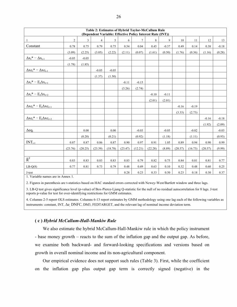
Our results provide strong support for such hybrid rules (Table 2). First, the coefficient

on the nominal income growth deviation term is negative in all cases consistent with a priori

expectations and is also statistically significant in most cases. This is true both for backward-

and forward-looking specifications. Second, the policy response is found to be stronger for

specifications using forward-looking versions (absolute long-run coefficient is 1.1-1.7) vis-a-

vis backward-looking specifications (0.4). Finally, in contrast to the conventional McCallum

rule and consistent with our results for the Taylor rule, the exchange rate coefficient is

wrongly signed and insignificant in all specifications.

 

26

Table 2: Estimates of Hybrid Taylor-McCallum Rule (Dependent Variable: Effective Policy Interest Rate (INT))

1 2 3 4 5 6 7 8 9 10 11 12 13

Constant 0.78 0.75 0.79 0.75 0.54 0.04 0.45 -0.37 0.49 0.14 0.38 -0.18

(3.09) (2.25) (3.05) (2.22) (2.11) (0.07) (1.61) (0.50) (1.76) (0.36) (1.16) (0.28)

Δxt* − Δxt-1 -0.05 -0.05

(1.78) (1.85)

Δxct* − Δxct-1 -0.05 -0.05

(1.37) (1.50)

Δxt* − EtΔxt+1 -0.11 -0.15

(3.26) (2.74)

Δxt* − EtΔxt+2 -0.10 -0.11

(2.01) (2.01)

Δxct* − EtΔxct+1 -0.16 -0.19

(3.33) (2.73)

Δxct* − EtΔxct+2 -0.16 -0.18

(1.92) (2.09)

Δeqt 0.00 0.00 -0.03 -0.05 -0.02 -0.03

(0.20) (0.21) (0.92) (1.18) (1.11) (0.93)

INTt-1 0.87 0.87 0.86 0.87 0.90 0.97 0.91 1.05 0.89 0.94 0.90 0.99

(23.76) (20.25) (23.39) (18.78) (23.47) (12.21) (22.28) (8.89) (20.57) (16.73) (20.57) (9.99)

R2

0.83 0.83 0.83 0.83 0.83 0.79 0.82 0.75 0.84 0.81 0.81 0.77

LB-Q(8) 0.77 0.81 0.73 0.79 0.48 0.49 0.63 0.10 0.32 0.48 0.60 0.25

J-test 0.28 0.23 0.33 0.50 0.23 0.18 0.30 0.37 1. Variable names are in Annex 1.

2. Figures in parenthesis are t-statistics based on HAC standard errors corrected with Newey-West/Bartlett window and three lags.

3. LB-Q test gives significance level (p-value) of Box-Pierce-Ljung Q-statistic for the null of no residual autocorrelation for 8 lags. J-test reports p-value for test for over-identifying restrictions for GMM estimates.

4. Columns 2-5 report OLS estimates. Columns 6-13 report estimates by GMM methodology using one lag each of the following variables as

instruments: constant, INT, Δe, DNFC, DM3, FEDTARGET, and the relevant lag of nominal income deviation term.

( c ) Hybrid McCallum-Hall-Mankiw Rule

We also estimate the hybrid McCallum-Hall-Mankiw rule in which the policy instrument

- base money growth – reacts to the sum of the inflation gap and the output gap. As before,

we examine both backward- and forward-looking specifications and versions based on

growth in overall nominal income and its non-agricultural component.

Our empirical evidence does not support such rules (Table 3). First, while the coefficient

on the inflation gap plus output gap term is correctly signed (negative) in the

27

contemporaneous versions, it is incorrectly signed in the forward-looking versions. In all

formulations, however, the coefficients are statistically insignificant. Second, consistent with

our findings for the McCallum rule, the exchange rate coefficient is correctly signed but

insignificant in all specifications.

Table 3: Estimates of Hybrid McCallum-Hall-Mankiw Rule (Dependent Variable: Growth in Base Money (Δbt))

1 2 3 4 5 6 7 8 9

Constant 5.28 5.64 5.24 5.58 6.21 5.85 6.46 5.88

(3.00) (3.94) (2.89) (3.73) (5.22) (4.97) (5.14) (4.68)

[(π – π*) + YGAP]t -0.01 -0.01

(0.08) (0.16)

[(πMPNF – π*MPNF) + YGAPC]

t -0.04 -0.06

(0.37) (0.62)

[(π – π*) + YGAP]t+1 0.12 0.10

(1.16) (0.90)

[(πMPNF – π*MPNF) + YGAPC]

t+1 0.08 0.03

(0.82) (0.29)

Δeqt-1 -0.04 -0.04 -0.03 -0.03

(1.42) (1.48) (1.33) (1.39)

Δbt-1 0.63 0.61 0.63 0.61 0.57 0.60 0.57 0.61

(5.49) (6.30) (5.32) (6.03) (7.10) (7.44) (6.81) (7.10)

R2

0.38 0.39 0.38 0.39 0.33 0.34 0.35 0.37

LB-Q(8) 0.11 0.13 0.11 0.13 0.14 0.12 0.15 0.14

J-test 0.72 0.68 0.71 0.64 1. Variable names are in Annex 1.

2. Figures in parenthesis are t-statistics based on HAC standard errors corrected with Newey-West/Bartlett window and three lags.

3. LB-Q test gives significance level (p-value) of Box-Pierce-Ljung Q-statistic for the null of no residual autocorrelation for 8 lags. J-test reports p-value for test for over-identifying restrictions for GMM estimates.

4. Columns 2-5 report OLS estimates. Columns 6-9 report estimates by GMM methodology using one lag each of the following variables as

instruments: constant, Δb, [(π – π*) + YGAP], [(πMPNF – π*MPNF) + YGAPC], Δe, DNFC, DM3, and FEDTARGET.

(d) Taylor Rule

In this paper, we refine and broaden the Taylor rule estimations conducted in the

context of operationalisation of the new Keynesian model in Indian conditions in Patra and

Kapur (2012). They estimated a monetary policy reaction function for India using the output

gap, inflation (measured by the y-o-y change either in the GDP deflator or in WPI inflation)

and the effective policy rate. Robustness properties were explored by estimating

28

contemporaneous and forward-looking versions of the Taylor rule and across alternative

sample periods.

At the outset of this sub-section, it is useful to set out a critical issue in the empirical

estimation of Taylor rules. The Taylor principle is that the long-run coefficient on the

inflation term should be more than unity. As pointed out in Section II, a coefficient of less

than unity implies that the real interest rate falls when inflation is rising, characteristic of the

policy mistakes found in the US in the 1960s and 1970s, and this will lead to even higher

inflation. Patra and Kapur (2012) show that the Taylor principle is amply satisfied in the

Indian context for forward-looking versions of the rule. For contemporaneous versions, the

long-run coefficient was found to be less than unity, thus violating the Taylor principle. In

contrast to Patra and Kapur (2012), others such as Anand et al (2010), Hutchison et al (2010)

and Mohanty and Klau (2004) obtained a long-run inflation coefficient less than unity. Patra

and Kapur (2012) suggested that this counter-Taylor principle result could be the outcome of

a number of factors such as (a) use of contemporaneous reaction functions, ignoring the

normal lags associated with the operation of monetary policy; (b) use of call money

rate/Treasury bill rate as a proxy for the policy rate; and (c) use of industrial output as the

activity variable rather than overall GDP.

In this paper, we empirically revisit this issue and in doing so, we examine additional

aspects such as: (a) use of actual GDP growth rates rather than the unobservable output gap;

(b) use of the output gap based on industrial GDP rather than overall GDP; (c) use of

provisional/preliminary data i.e., data actually used by the central bank at the time of taking

policy action) and not the revised estimates14; (d) using the RBI’s monetary policy

projections for growth and inflation (semi-annual up to mid-2005 and quarterly thereafter),

which can obviate the need for use of instruments and, therefore, estimable by OLS; (e) use

of non-food manufactured products WPI inflation (in lieu of headline inflation) recently

articulated by the Reserve Bank as an indicator of core demand pressures and the non-

agricultural output gap to abstract from volatility caused by supply shocks; and (f) use of the

call money rate instead of the effective policy rate. For the various potential combinations,

14 Orphanides (2003) suggests that the results can be sensitive to the vintage of the data  

29

we present results for both forward-looking and contemporaneous specifications. In all cases,

we also assess as to whether exchange rate dynamics play any role in the policy reaction

functions.

The results for these alternative explanatory variables/combinations are presented in

Tables 4 and 5. The main findings are summarized below: First, the estimation results

obtained in Patra and Kapur (2012) are robust to using various alternative indicators of

inflation and growth.

Second, the coefficients on inflation and output gap terms are statistically significant and

satisfy the Taylor principle in almost all the forward-looking specifications (Table 4). The

coefficient estimates indicate stronger policy response to non-food manufactured products

inflation dynamics, consistent with the Reserve Bank’s recent emphasis on this indicator of

underlying demand pressures in the context of the 2010-11 inflation episode.

Third, the only instance in the forward-looking specifications when the coefficient on the

inflation term is insignificant is when we use call rate as the policy instrument in lieu of the

effective policy rate (Table 4, columns 14-15). Moreover, the R2 drops substantially to 0.26

vis-à-vis 0.80-0.90 in the specifications using the effective policy rate. Over the period of

evolution of the current monetary policy regime in India, there have been brief periods when

the call rate has exhibited significant volatility and has moved significantly away from the

policy corroder set by the repo and the reverse repo rate.

30

Table 4: Estimates of Taylor Rule (Forward-looking Specifications) (Dependent Variable: Effective Policy Interest Rate (INT))

1 2 3 4 5 6 7 8 9 10 11 12 13 14 15

Constant 0.64 0.58 -1.45 -1.45 0.46 0.51 0.41 -0.03 -0.21 -0.43 0.50 0.34 1.72 2.66 (2.41) (1.20) (1.99) (1.96) (2.06) (1.67) (1.87) (0.08) (0.60) (1.08) (2.16) (1.06) (3.10) (2.18)

(π – π*)t+2 0.16 0.15 0.11 0.10 0.15 0.15 (2.63) (2.10) (2.62) (1.83) (2.51) (2.38)

YGAP t+2 0.18 0.17 (2.16) (1.60)

(πPROV -π*)t+2 0.09 0.09 (1.72) (1.49)

GDPPROJ{+1} 0.26 0.26 (3.07) (3.29)

(πMPNF – π*MPNF)t+2 0.21 0.21

(5.23) (5.02)

YGAPC t+2 0.15 0.16

(2.75) (2.01)

(π – π*)t+1 0.14 0.19 0.17 0.09 (4.50) (4.04) (2.28) (1.09)

Δ(YGAP) t+2 0.37 0.31 (1.50) (0.85)

GDPRG 0.06 0.07 (1.70) (1.80)

YGAPINDt+2 0.11 0.10

(2.82) (2.60)

YGAPt+1 0.48 0.48 (2.68) (2.18)

Δet -0.01 0.00 0.00 -0.03 -0.01 -0.01 0.08 (0.29) (0.11) (0.27) (2.13) (0.86) (0.89) (1.86)

INTt-1 0.88 0.89 0.94 0.94 0.91 0.91 0.92 0.99 0.95 0.98 0.91 0.93 (24.02) (11.90) (34.87) (24.89) (29.54) (18.84) (27.61) (18.74) (28.52) (18.46) (26.95) (19.30)

CALLt-1 0.71 0.58 (7.67) (3.03)

R2

0.85 0.84 0.90 0.90 0.86 0.86 0.82 0.81 0.85 0.84 0.84 0.83 0.26 0.32 LB-Q(8) 0.79 0.79 0.76 0.75 0.57 0.57 0.75 0.41 0.67 0.63 0.66 0.56 0.70 0.80 J-test 0.55 0.44 0.71 0.64 0.68 0.64 0.57 0.47 0.56 0.54 0.77 0.71

Long-run coefficients

Inflation 1.33 1.40 1.45 -- 2.43 2.24 1.77 16.14 2.39 4.73 1.60 2.28 0.58 -- Output 1.51 1.58 4.16 4.25 1.71 1.71 -- -- 1.21 3.12 1.18 1.53 1.69 1.15

Note: 1. Variable names are in Annex 1. 2. Figures in parenthesis are t-statistics based on HAC standard errors corrected with Newey-West/Bartlett window and three lags. 3. LB-Q test gives significance level (p-value) of Box-Pierce-Ljung Q-statistic for the null of no residual autocorrelation for 8 lags. J-test reports p-value for test for over-identifying restrictions for GMM estimates. 4. Estimation is by GMM methodology for the sample period 1997:2 to 2011:1 using one lag each of the following variables as instruments: int, ygap, , , , INFG, oil, Δe, DNFC, DM3 and fedtarget for the specification in columns 2-3 and 6-15; for columns 14 and 15, the instrument ‘int’ is replaced by ‘call’. Columns 4 and give are OLS estimates.

31

Table 5: Estimates of Taylor Rule (Contemporaneous Specifications) (Dependent Variable: Effective Policy Interest Rate (INT))

1 2 3 4 5 6 7 8 9 10 11 12 13 14 15 16 17

Constant 0.61 0.53 0.63 0.58 0.51 0.43 0.01 -0.01 -0.41 -0.46 -0.55 -0.56 0.74 0.73 3.84 4.06 (2.60) (1.92) (2.21) (1.81) (2.39) (1.49) (0.03) (0.03) (0.64) (0.81) (1.38) (1.49) (3.10) 3.01 4.46 4.90

(π – π*)t 0.07 0.08 0.09 0.10 0.08 0.08 0.06 0.06 0.08 0.03 (3.37) (2.80) (3.47) (2.88) (3.19) (2.63) (1.79) (1.79) (0.78) (0.28)

YGAPt 0.19 0.19 0.50 0.53 (2.88) (3.09) (3.08) (2.95)

(πMPNF – π*MPNF)t 0.06 0.06 (1.89) (1.83)

YGAPC t 0.31 0.31

(3.15) (3.05)

Δ(YGAP) t 0.08 0.08 (1.26) (1.22)

GDPRG 0.08 0.08 (2.15) (2.51)

INFWPIPROJDEV 0.20 0.20

(2.21) (1.85)

GDPPROJ 0.13 0.13 (1.53) (1.71)

(πPROV -π*)t 0.08 0.09 (3.08) (2.37)

GDPRGPRELIM 0.16 0.15

(2.50) (2.77)

YGAPINDt 0.18 0.17

(1.83) (2.16)

Δeqt -0.01 -0.01 -0.01 0.00 -0.01 -0.01 0.00 0.05 (0.61) (0.54) (0.56) (0.27) (0.45) (0.54) (0.07) (1.90)

INTt-1 0.90 0.91 0.90 0.91 0.91 0.92 0.90 0.90 0.91 0.92 0.89 0.91 0.88 0.88 (24.7) (24.4) (20.7) (19.9) (29.7) (25.6) (29.4) (25.0) (31.1) (30.1) (15.5) (23.1) (23.4) (25.0)

CALLt-1 0.40 0.36 (3.67) (3.32)

R2

0.90 0.90 0.91 0.91 0.89 0.89 0.86 0.85 0.90 0.90 0.82 0.82 0.91 0.91 0.35 0.39 LB-Q(8) 0.95 0.93 0.79 0.81 0.79 0.85 0.86 0.87 0.76 0.77 0.51 0.59 0.74 0.74 0.77 0.84

Long-run coefficients Inflation 0.70 0.90 0.55 0.65 0.99 1.26 0.77 0.86 2.12 2.42 0.74 0.95 0.47 0.48 --- --- Output 1.86 2.04 3.02 3.34 -- -- 0.75 0.77 -- 1.58 1.48 1.58 1.45 1.45 0.83 0.83

1. Variable names are in Annex 1.

2. Figures in parenthesis are t-statistics based on HAC standard errors corrected with Newey-West/Bartlett window and three lags.

3. LB-Q test gives significance level (p-value) of Box-Pierce-Ljung Q-statistic for the null of no residual autocorrelation for 8 lags.

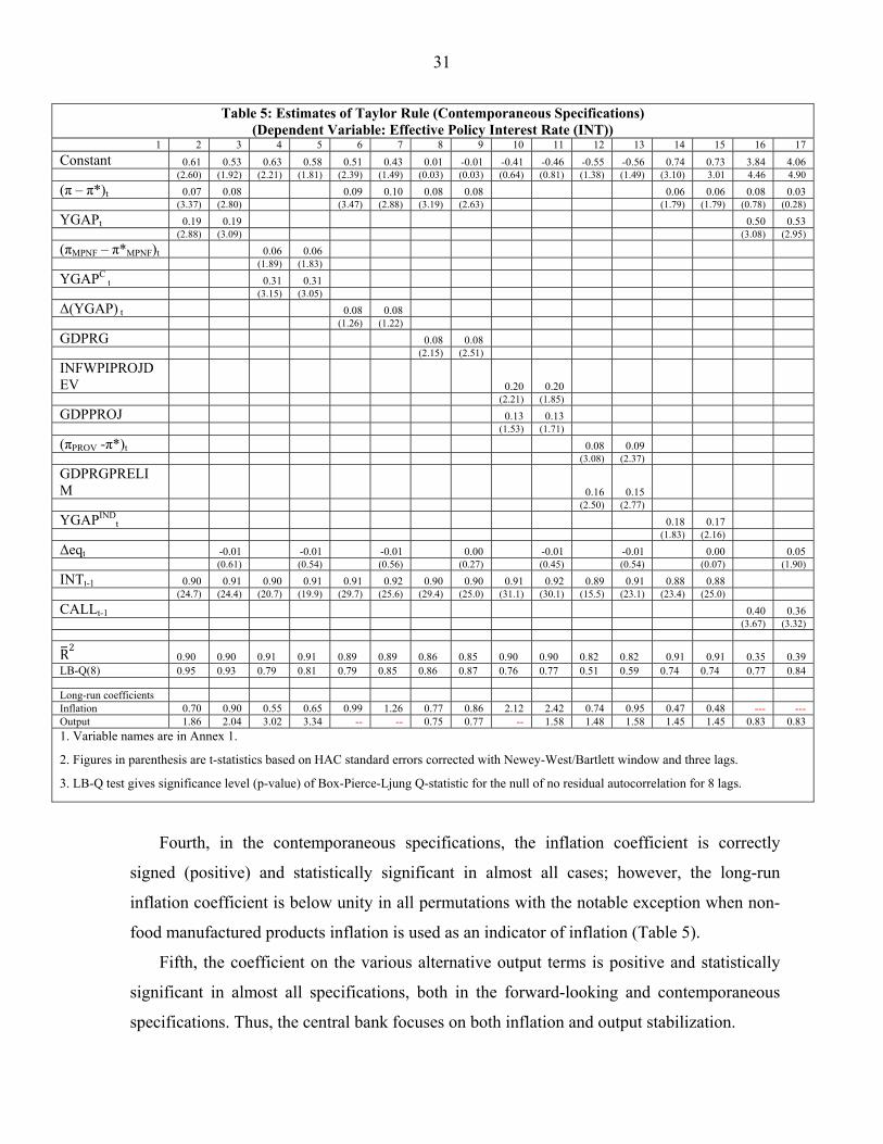
Fourth, in the contemporaneous specifications, the inflation coefficient is correctly

signed (positive) and statistically significant in almost all cases; however, the long-run

inflation coefficient is below unity in all permutations with the notable exception when non-

food manufactured products inflation is used as an indicator of inflation (Table 5).

Fifth, the coefficient on the various alternative output terms is positive and statistically

significant in almost all specifications, both in the forward-looking and contemporaneous

specifications. Thus, the central bank focuses on both inflation and output stabilization.

32

Sixth, turning to the issue of whether the monetary authority uses the interest rate

instrument to lean against exchange rate volatility, the coefficient is found to be wrongly

signed and insignificant in all instances. This is true for both the forward-looking and the

contemporaneous specifications (Tables 4-5). The results are consistent with the WPI

inflation specifications in Patra and Kapur (2012). The only instance in which the exchange

rate variable enters the regression with the correct sign (positive) is when the call rate is used

as the policy rate; however, when we use the call rate, the inflation terms, as noted earlier,

lose significance. The exchange rate variable being insignificant in the policy reaction

function appears to reflect the RBI’s approach to exchange rate management. The exchange

rate regime in India has been described as a "bounded float" (Gokarn, 2012) under which the

exchange rate is determined by daily variations in demand and supply and in excessively

volatile market conditions, "smoothing" interventions help to keep markets orderly and

prevent large jumps that can induce further spirals. Notably, the use of policy interest rates to

target any level or band of the exchange rate is never resorted to.

Finally, the alternative specifications in the forward-looking version indicate that the

neutral policy rate is around 5.5 per cent.

(e) Alternative Interest Rate Rules in the Literature

Even as the Taylor rule has come to be widely regarded as the most representative

way of defining modern-day monetary policy reaction functions, there remains significant

disagreement about several issues around it. Perhaps the most visited of these contentious

themes has been that of the weights on the various coefficients. While there is unanimity that

the long-run coefficient on the inflation term should be more than unity, there are a range of

opinions regarding other variables in the rule – whether there should be any weight on the

output gap term at all; whether there should be interest rate smoothing; and so forth. An

assessment of these views is dependent upon the model of the economy that the rule is nested

in, and the superiority of one rule over another could be model-dependent. Influential work

on the consolidation of work on alternative monetary policy rules has assessed five different

policy rules for robustness (Taylor, 1999a). They are reproduced below:

33

Table 6: Alternative Taylor-type Monetary Policy Rules

Rule Coefficient on

Inflation gap Output gap Lagged interest rate

1 2 3 4

I 3.0 0.8 1.0

II 1.2 1.0 1.0

III 1.5 0.5 0.0

IV 1.5 1.0 0.0

V 1.2 0.06 1.3

Rules I and II (interest-rate smoothing rules) have the interest rate reacting to the

lagged interest rate with a response coefficient of one. Rule I has a high weight on inflation

compared to the weight on output, and Rule II has a smaller weight on inflation compared to

Rule I, but a relatively higher weight on output. Rule III is the simple rule proposed by

Taylor (1993) without any interest rate smoothing. Rule IV is on the same lines as Rule III

but with a coefficient on real output that is twice as high. Rule V, suggested in Rotemberg

and Woodford (1999), places a very small weight on real output and a very high weight on

the lagged interest rate. Rule VI is the forward-looking rule estimated in this paper (Table 4,

column 2).

For the purpose of complete simulation of the alternative policy rules within the new

Keynesian model, we update the preferred specifications of aggregate demand and aggregate

supply functions in Patra and Kapur (2012). The estimated equations are as below (t-statistics

are in parentheses; LB-Q(8) gives p-value of Box-Pierce-Ljung Q-statistic for the null of no

residual autocorrelation for 8 lags):

YGAPt = 0.08 – 0.06*RIRt-2 + 0.49*YGAPt-1 + 0.40*WYGAPt – 0.10*RERt-2 + 1.81*D01:4 - 1.91*D02:4 - 2.07*D04:1 (1.1) (1.9) (6.9) (7.3) (3.6) (10.7) (9.1) (24.5)

R2 = 0.74 LB-Q (8) = 0.45

πt = 2.18 + 0.19*YGAPt-1 + 0.95*πt-1 - 0.44*πt-2 + 0.07*INFGt + 0.06*EXCHAt + 3.32*D98:3

(5.9) (2.0) (14.1) (5.2) (4.2) (2.5) (3.7)

R2 = 0.82 LB-Q (8) = 0.21

where, YGAP, RIR, WYGAP, RER, π, INFG, and EXCHA are the output gap, real

interest rate (= nominal effective policy rate less y-o-y WPI inflation), global output gap, real

effective exchange rate gap, WPI inflation (y-o-y), international non-fuel commodity price

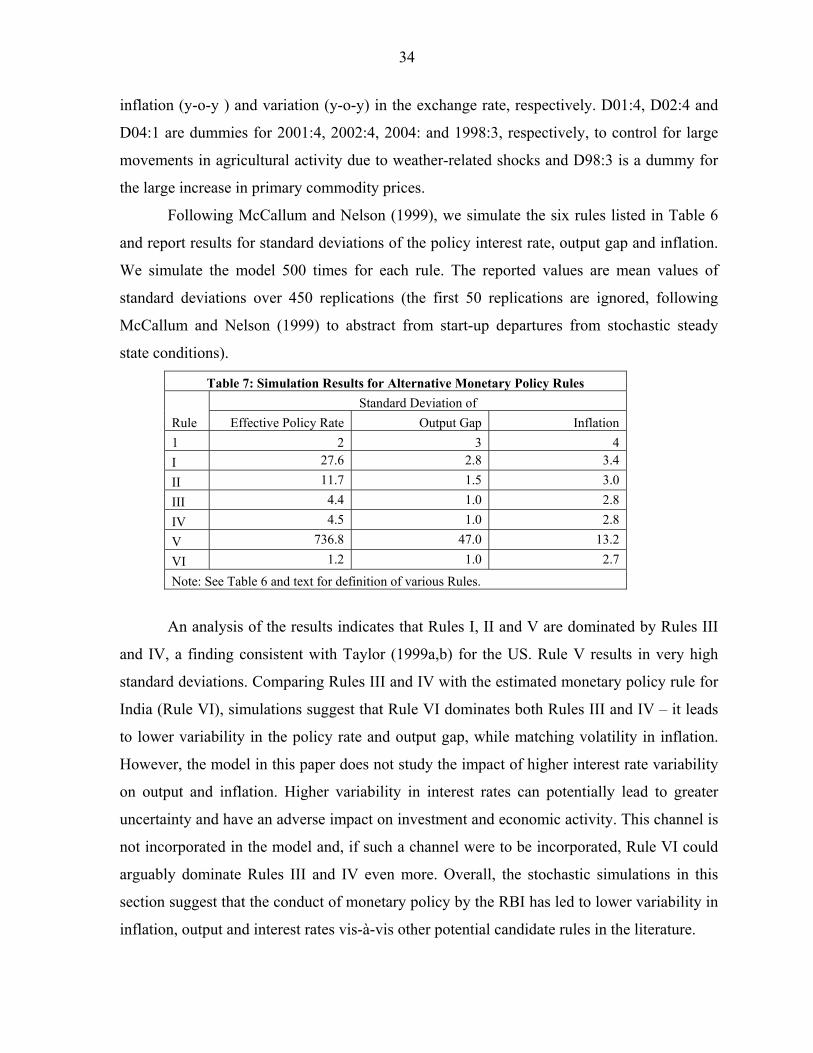
34

inflation (y-o-y ) and variation (y-o-y) in the exchange rate, respectively. D01:4, D02:4 and

D04:1 are dummies for 2001:4, 2002:4, 2004: and 1998:3, respectively, to control for large

movements in agricultural activity due to weather-related shocks and D98:3 is a dummy for

the large increase in primary commodity prices.

Following McCallum and Nelson (1999), we simulate the six rules listed in Table 6

and report results for standard deviations of the policy interest rate, output gap and inflation.

We simulate the model 500 times for each rule. The reported values are mean values of

standard deviations over 450 replications (the first 50 replications are ignored, following

McCallum and Nelson (1999) to abstract from start-up departures from stochastic steady

state conditions).

Table 7: Simulation Results for Alternative Monetary Policy Rules

Rule

Standard Deviation of

Effective Policy Rate Output Gap Inflation

1 2 3 4

I 27.6 2.8 3.4

II 11.7 1.5 3.0

III 4.4 1.0 2.8

IV 4.5 1.0 2.8

V 736.8 47.0 13.2

VI 1.2 1.0 2.7

Note: See Table 6 and text for definition of various Rules.

An analysis of the results indicates that Rules I, II and V are dominated by Rules III

and IV, a finding consistent with Taylor (1999a,b) for the US. Rule V results in very high

standard deviations. Comparing Rules III and IV with the estimated monetary policy rule for

India (Rule VI), simulations suggest that Rule VI dominates both Rules III and IV – it leads

to lower variability in the policy rate and output gap, while matching volatility in inflation.

However, the model in this paper does not study the impact of higher interest rate variability

on output and inflation. Higher variability in interest rates can potentially lead to greater

uncertainty and have an adverse impact on investment and economic activity. This channel is

not incorporated in the model and, if such a channel were to be incorporated, Rule VI could

arguably dominate Rules III and IV even more. Overall, the stochastic simulations in this

section suggest that the conduct of monetary policy by the RBI has led to lower variability in

inflation, output and interest rates vis-à-vis other potential candidate rules in the literature.

35

V. Summary and Conclusion

Rules versus discretion? The debate will continue to generate heat, dust but also,

importantly, light. As long as uncertainty is their stock-in-trade, central banks and monetary

authorities will regard some discretion as their due. Nevertheless, policy outcomes can

arguably tend towards optimal if that discretion is evaluated against some sense of a rule

even if it is at the back of an envelope. Or even better, against a suite of alternative policy

rules. From a practical perspective, easy operability and a reasonably accurate description of

reality will obviously have to be features of this effort for it to be meaningful enough to

engage monetary authorities.

In this paper, we empirically assessed the McCallum Rule and the Taylor Rule under

Indian conditions as alternatives rather than as competing guideposts for the operational

conduct of monetary policy. This is in itself a difficult task. Each is replete with

methodological nuances that have been intensively researched enough to set them up against

each other. While one has found appeal because it more realistically portrays modern-day

monetary policy, the other enables the balancing of multiple objectives while avoiding

unobservables that have measurement issues in real life, despite their empirical elegance.

Cross-fertilisation yielded results that comparable to thorough-breds and their extensions.

Both Rules apply to the monetary policy framework in India as it has evolved over the past

one and a half decades – while the interest rate is the main policy instrument currently, its

impact on the rest of the economy continues to be conveyed by modulating bank reserves or

adjusted reserve money.

Our results can be best summarized as follows: first, a forward-looking McCallum

Rule in which the reserve money changes react to changes in non-agricultural output gap

with a significant degree of instrument smoothing outperforms other base money rules.

Second, the forward-looking hybrid McCallum Rule using the interest rate as the policy

instrument reacting to movements in non-agricultural output gap is strongly supported by the

data in explaining the conduct of Indian monetary policy. Third, a forward-looking Taylor

Rule with the effective policy interest rate (repo rate or reverse repo rate depending on

liquidity conditions) reacting to non-food manufacturing inflation and the two-period ahead

output gap – overall and/or non-agricultural – appears best suited to Indian conditions among

36

interest rate rules. Fourth, exchange rate movements do not play a significant role in policy

setting, and typically evoke only lagged quantity adjustments. Finally, simulation exercises

indicate that the interest rate reaction function followed by the RBI dominates alternative

Taylor rules recommended in the literature as it yields lower variability of inflation, output

and interest rate.

The empirical results of this paper suggest that there is scope for future work by

extending the simulation analysis for Taylor-like rules in this paper to McCallum and the

hybrid Rules and to compare the outcomes for volatility in inflation and output across

alternative rules. Such an exercise would throw light on the question as to whether setting a

nominal output growth objective a la McCallum or whether responding to inflation and

output developments in a flexible manner a la Taylor combine the best parts of efficiency

and discretion.

37

References Anand, Rahul, Shanaka Peiris and Magnus Saxegaard, 2010, “An Estimated Model with Macrofinancial Linkages for India”, Working Paper WP/10/21, International Monetary Fund. Ball, Laurence, 1999, "Policy Rules for Open Economies" in John B. Taylor (ed.), 1999, Monetary Policy Rules, University of Chicago Press, Chicago, pp. 127-156. Barro, Robert J and Gordon, David B, 1983, "A Positive Theory of Monetary Policy in a Natural Rate Model", Journal of Political Economy, Vol. 91(4), August, pp. 589-610. Blattner, Tobias S. and Emil Margaritov, 2010, “Towards a Robust Monetary Policy Rule for the Euro Area”, Working Paper 1210, European Central Bank. Brayton, Flint, Andrew Levin, Ralph Tryon, and John Williams, 1997, The Evolution of Macro Models at the Federal Reserve Board, Carnegie-Rochester Conference Series on Public Policy, Vol. 47 (1), pp. 43-81. Carlson, John B., 1988, “Rules Versus Discretion: Making a Monetary Rule Operational”, Economic Review, Federal Reserve Bank of Cleveland, Issue Q III, pp.2-13. Clarida, Richard, Jordi Gali and Mark Gertler, 1998, “Monetary Policy Rules in Practice: Some International Evidence”, European Economic Review, Vol.42, pp.1033-1067. -------, 2000, “Monetary Policy Rules and Macroeconomic Stability: Evidence and Some Theory”, Quarterly Journal of Economics, Vol. 115, pp. 147-180. Central Statistical Organisation, Government of India at http://www.mospi.gov.in/mospi_press_releases.htm Croushore, Dean and Tom Stark, 1996, "Evaluating McCallum's rule when monetary policy matters," Working Paper 96-3, Federal Reserve Bank of Philadelphia Diez de los Rios, A., 2009, McCallum Rules, Exchange Rates, and the Term Structure of Interest Rates, Working Paper 08-43, Bank of Canada. Dueker, Michael J., 1993, "Can Nominal GDP Targeting Rules Stabilize the Economy?", Review, May/June, Federal Reserve Bank of St. Louis, pp. 31-40. Esanov, A., C. Merkl and l. Vinhas de Souza, 2004, “Monetary Policy Rules for Russia”, Discussion Papers 11, Bank of Finland. Federal Reserve Bank of St. Louis, Fred Database, at http://research.stlouisfed.org/fred2/ Feldstein, Martin, 1999, Comment, in John B. Taylor (ed.), 1999, Monetary Policy Rules, University of Chicago Press, Chicago, pp, 119-123.

38

Fischer, Stanley, 1988, “Rules Versus Discretion in Monetary Policy”, Working Paper 2518, National Bureau of Economic Research. Friedman, M., 1960, A Program for Monetary Stability, Fordham University Press, New York. Gokarn, Subir, 2012, “An Assessment of Recent Macroeconomic Developments”, Reserve Bank of India Bulletin, January. Goodfriend, Marvin, 2000. "Overcoming the Zero Bound on Interest Rate Policy," Journal of Money, Credit and Banking, Vol. 32(4), pp. 1007-35. Hall Thomas E., 1990, “McCallum’s Base Growth Rule: Results for the United States, West Germany, Japan and Canada”, Weltwirtschaftliches Archiv, Vol. 126 (4), pp. 630-642. Hall, R.E. and N.G. Mankiw, 1993, "Nominal Income Targeting," in N.G. Mankiw, (ed.), Monetary Policy, University of Chicago Press, Chicago, pp. 71-93. Haslag, Joseph H., and Scott E. Hein, 1995, “Does it Matter How Monetary Policy is Implemented?”, Journal of Monetary Economics, Vol. 35 (2), pp. 359-386. Hutchison, Michael, Rajeswari Sengupta and Nirvikar Singh, 2010, “Estimating a Monetary Policy Rule for India”, Economic and Political Weekly, September 28, Vol. XLV (38), pp. 67-69 Inoue, Takeshi and Shigeyuki, Hamori, 2009, “An Empirical Analysis of the Monetary Policy Reaction Function in India,” Discussion Paper 200, Institute of Developing Economies. Jha, Raghbendra, 2008, "Inflation Targeting in India: Issues and Prospects", International Review of Applied Economics, Vol. 22(2), pp.259-270. Judd, John P. and Brian Motley, 1991, “Nominal Feedback Rules for Monetary Policy”, Economic Review, Summer, Federal Reserve Bank of San Francisco, pp. 3-17 -----, 1993, “Using a Nominal GDP Rule to Guide Discretionary Monetary Policy”, Economic Review, Vol. 3, Federal Reserve Bank of San Francisco, pp. 3-11. Khakimov, Obid, Levent Erdogan and Nilgun Caglarirmak Uslu, 2009, “Assessing Monetary Policy Rule in Turkey”, Paper presented at EconAnadolu 2009: Anadolu International Conference in Economics, June 17-19, Eskisehir, Turkey. Koivu, Tuuli, Aaron Mehrotra and Riikka Nuutilainen, 2008, “McCallum Rule and Chinese Monetary Policy”, Working Paper, Bank of Finland. Krugman, Paul, 1998, “Its Baaack: Japan’s Slump and the Return of the Liquidity Trap”, Brookings Paper on Economic Activity, No 2, pp. 137-205.

39

Kydland, Finn and Edward Prescott, 1977, “Rules Rather than Discretion: The Inconsistency of Optimal Plans”, Journal of Political Economy, Vol. 85 (3), pp. 473-492. Lucas, Robert E, Jr, 1975, "An Equilibrium Model of the Business Cycle," Journal of Political Economy, Vol. 83(6), December, pp. 1113-1144. --------------------, 1980, "Rules, Discretion, and the Role of the Economic Advisor" in Stanley Fischer (ed.), 1980, Rational Expectations and Economic Policy, University of Chicago Press, Chicago, pp. 199-210. McCallum, Bennett T., 1987, “The Case for Rules in the Conduct of Monetary Policy: A Concrete Example”, Economic Review, September/October, Federal Reserve Bank of Richmond, pp. 10-18. ------, 1988, Robustness Properties of A Rule for Monetary Policy, Carnegie-Rochester Conference Series on Public Policy, Vol. 29 (1), pp. 173-203. ------, 1990, “Targets, Indicators and Instruments of Monetary Policy”, in W. Haraf and W.Cagan (eds.), Monetary Policy for a Changing Financial Environment, AEI Press, Washington DC, pp. 44-70. ------, 1993, “Specification and Analysis of A Monetary Policy Rule for Japan”, Working Paper 4449, National Bureau of Economic Research. ------, 2000, “Alternative Monetary Policy Rules: A Comparison with Historical Settings for the United States, the United Kingdom, and Japan," Working Paper 7725, National Bureau of Economic Research. ------, 2002, “Recent Developments in Monetary Policy Analysis: The Roles of Theory and Evidence," Economic Quarterly, Winter Issue, Federal Reserve Bank of Richmond, pp. 67-96. ------, and Edward Nelson, 1999, "Nominal Income Targeting in an Open-Economy Optimizing Model," Journal of Monetary Economics, Vol. 43(3), pp. 553-578. Meade, J.E., 1978, “The Meaning of Internal Balance”, Economic Journal, Vol. 88(351), pp. 423-435. Mehrotra, Aaron and Jose R. Sanchez-Fung, 2011, “Assessing McCallum and Taylor Rules in a Cross-section of Emerging Market Economies”, Journal of International Financial Markets, Institutions and Money, Vol. 21, pp. 207-228. Meltzer, Allan, H., 1998, “Time to Print Money,” Financial Times, July 17 Mohanty, Deepak (2011), “How does the Reserve Bank of India Conduct its Monetary Policy?”, Reserve Bank of India Bulletin, September.

40

Mohanty, Deepak, A. B. Chakraborty, Abhiman Das and Joice John (2011), “Inflation Threshold in India: An Empirical Investigation”, Working Paper (DEPR) 18/2011, Reserve Bank of India. Mohanty, M.S. and Marc Klau, 2004, “Monetary Policy Rules in Emerging Market Economies: Issues and Evidence”, Working Paper 149, Bank for International Settlements. Orphanides, Athanasios, 2003, “Historical Monetary Policy Analysis and the Taylor Rule”, Journal of Monetary Economics, Vol. 50 (5), pp. 983-1022. --------, 2007, “Taylor Rules”, Working Paper FEDS 2007-18, Board of Governors of the Federal Reserve System, January. Paez-Farrell, Juan, 2009, “Monetary Policy Rules in Theory and in Practice: Evidence from the UK and the US”, Applied Economics, Vol. 41(16), pp. 2037-2046 Patra, M.D., and Muneesh Kapur, 2012, “A Monetary Policy Model for India”, Macroeconomics and Finance in Emerging Market Economies, Vol. 5(1), pp. 16-39. Pattanaik, Sitikantha and G. V. Nadhanael (2011), “Why Persistent High Inflation Impedes Growth? An Empirical Assessment of Threshold Level of Inflation for India” Working Paper (DEPR) 17/2011, Reserve Bank of India. Rangarajan, C and Anoop Singh, 1984, “Reserve Money: Concepts and Implications for India”, Occasional Papers, Reserve Bank of India. Rangarajan, C., 1985, “Money, Output and Prices”, S.K. Murunjan Memorial Lecture, 1985. -----, 1988, Issues in Monetary Management, Presidential Address at the 71st Annual Conference of the Indian Economic Association, Jadavpur University, Calcutta, December. -----, 1993, “Autonomy of Central Banks”, Tenth M.G. Kutty Memorial Lecture, Calcutta, September. -----, 1997, “The Changing Context of Monetary Policy”, Address at the 31st Convocation of the Indian Statistical Institute, Calcutta, March. ----------, 2001, “Some Critical Issues in Monetary Policy”, Economic and Political Weekly, June 16. Razzak, W. A., 2003, “Is The Taylor Rule Really Different From The McCallum Rule?”, Contemporary Economic Policy, Vol. 21, No. 4 Reserve Bank of India (2011), Handbook of Statistics on the Indian Economy 2010-11.

41

Rogoff, Kenneth, 1985. "The Optimal Degree of Commitment to an Intermediate Monetary Target," Quarterly Journal of Economics, Vol. 100(4), pp. 1169-89. Rotemberg, Julio J., and Michael Woodford, 1999, “Interest Rules in an Estimated Sticky Price Model”, in John B. Taylor (ed.), 1999, Monetary Policy Rules, University of Chicago Press, Chicago, pp. 57-126. Rudebusch, Glenn, and Lars Svensson, 1999, “Policy Rules for Inflation Targeting”, in John B. Taylor (ed.), 1999, Monetary Policy Rules, University of Chicago Press, Chicago, pp. 203–62. Simons, Henry C., 1936, “Rules Versus Authorities in Monetary Policy”, Journal of Political Economy, Vol. 44 (1), pp. 1-30. Singh, Bhupal, 2010, “Monetary Policy Behavior in India: Evidence from Taylor-type Policy Frameworks”, Staff Studies, SS(DEAP) 2/2010, Reserve Bank of India. Singh, Kanhaiya, 2006, "Inflation Targeting: International Experience and Prospects for India", Economic and Political Weekly, Vol. 41 (27-28), pp.2958-2961 Sun, Shuzhang, Christopher Gan and Baidung Hu, 2010, “Evaluating McCallum Rule as Policy Guidelines for China”, Joint Annual Conference of the New Zealand Association of Economics and Lae and Economics Association of New Zealand, June 30-July 2, 2010. Taylor, John B., 1993, “Discretion versus Policy Rules in Practice”, Carnegie-Rochester Conference Series on Public Policy, Vol. 39, pp. 195-214. -----, 1999a, "Introduction” in John B. Taylor (ed.), 1999, Monetary Policy Rules, University of Chicago Press, Chicago, pp. 1-14. -----, 1999b, "A Historical Analysis of Monetary Policy Rules," in John B. Taylor (ed.), 1999, Monetary Policy Rules, University of Chicago Press, Chicago, pp. 319-348. ------, 2000, "The Monetary Transmission Mechanism and the Evaluation of Monetary Policy Rules," Working Paper 87, Central Bank of Chile. ------ and John. C. Williams, 2010, “Simple and Robust Rules for Monetary Policy”, Working Paper 15908, National Bureau of Economic Research. Tobin, J., 1980, “Stabilisation Policy Ten Years After”, Brookings Papers on Economic Activity, No. 1. Virmani, Vineet, 2004, “Operationalsing Taylor-type Rules for the Indian Economy: Issues and Some Results”, Working Paper 2004-07-04, ICICI Research Center and Institute for Financial Management and Research, Chennai, India

42

Walsh, Carl E., 1995, “Optimal Contracts for Central Bankers”, American Economic Review, Vol. 85, No. 1, March, pp. 150-167. Wicksell, Knut, 1898, Interest and Prices. A Study of the Causes Regulating the Value of Money, London: Macmillan. Woodford, Michael, 2003, Interest and Prices: Foundations of a Theory of Monetary Policy, Princeton University Press.

43

Annex I: List of Variables CALL = Overnight call money rate

CRR = Cash reserve ratio

DLM3 = Variation (y-o-y) in broad money (M3)

DLNFC = Variation (y-o-y) in non-food credit

EXCHA = Variation (y-o-y) in exchange rate of the Rupee vis-a-vis the US dollar

FEDFUND = US Federal Funds rate target

GDPPROJ = RBI’s monetary policy projection for real GDP growth (year-on-year)

GDPRG = Real GDP growth (year-on-year)

GDPRGPREL = Real GDP growth (year-on-year) based on preliminary data

INFG = International commodity price inflation (year-on-year) (measured by IMF’s non-fuel index in US $ terms)

INT = Effective nominal policy rate (as defined in text)

REERGAP = real exchange rate gap = 36-currency real effective exchange rate (seasonally adjusted) less its HP filtered series

RPR = Real policy rate (nominal effective policy rate less y-o-y WPI inflation)

YGAP = Output gap = Real GDP (seasonally adjusted) less its HP filtered series

YGAPC = Non-agricultural output gap = Real non-agricultural GDP (seasonally adjusted) less its HP filtered series YGAPIND = Industrial output gap = Real industrial GDP (seasonally adjusted) less its HP filtered series

Δb = Growth (y-o-y) in reserve money (adjusted for CRR changes)

Δe = Variation (q-o-q, annualized) in exchange rate of the Rupee vis-a-vis the US dollar

Δx = Growth (y-o-y) in nominal GDP

Δx* = Trend growth (y-o-y) in nominal GDP

Δxc = Growth (y-o-y) in non-agricultural nominal GDP

Δxc* = Trend growth (y-o-y) in non-agricultural nominal GDP

π = Wholesale price index (WPI) inflation (year-on-year)

π* = Monetary policy inflation objective (taken as 5 per cent)

πMPNF = Non-food manufactured products WPI inflation (year-on-year)

π*MPNF = Monetary policy objective for non-food manufactured products inflation (taken as 4 per cent)

πPROV = Provisional wholesale price inflation (year-on-year)

πPROJ = RBI’s monetary policy projection for wholesale price inflation (year-on-year)

= Deviation of consumer price inflation (year-on-year) from policy objective

= Deviation of GDP deflator inflation (year-on-year) from policy objective

Note: All data are in percentages.