alternative methods for estimating full marginal costs of highway transportation

Transportation Research Part A 41 (2007) 768–786

www.elsevier.com/locate/tra

Alternative methods for estimating full marginal costsof highway transportation

Kaan Ozbay a, Bekir Bartin a,*, Ozlem Yanmaz-Tuzel a, Joseph Berechman b

a Civil and Environmental Engineering Department, Rutgers University, 623 Bowser Road, Piscataway, NJ 08854, United Statesb Sauder School of Business and SCARP, The University of British Columbia, Vancouver, BC, Canada

Abstract

This paper presents various methods of estimating the full marginal cost (FMC) of highway passenger transportation.First, the computation of FMC is performed using the marginal cost functions, most of which were developed by Ozbayet al. [Ozbay, K., Bartin, B., Berechman, J., 2001. Estimation and evaluation of full marginal costs of highway transpor-tation in New Jersey. Journal of Transportation and Statistics 4 (1)]. FMC is defined and calculated as ‘‘total cost per trip’’as explained in this paper. However, in multiple origin-destination and multiple route highway networks, the practicalapplication of the network-wide FMC concept is complicated. These issues are addressed in detail in this paper. Therefore,in the second method, a multiple route based FMC approach is proposed for a given origin-destination pair in the net-work. It is observed that the marginal values of different paths vary as much as 28%. Third, a comparison of FMC esti-mation results of two distinct measurement tools is presented. The FMC estimation is performed between a selected ODpair using the static transportation planning software output (TransCAD). The same analysis is repeated using the stochas-tic traffic simulation software output (PARAMICS). The differences in FMC values estimated by static transportationplanning software and microscopic traffic simulation software are discussed.� 2007 Elsevier Ltd. All rights reserved.

Keywords: Marginal cost; Transportation economy; Highway costs; Simulation

1. Background and objectives

At the heart of many congestion mitigation options lies the accurate estimation of full marginal highwaytravel costs accrued to the State. This information is essential for allocating resources efficiently, for ensuringequity among users of different transportation modes, and for developing an effective pricing mechanism. FullMarginal Cost (FMC) means the overall costs accrued to society from servicing an additional unit of traffic.FMC includes vehicle operating costs, infrastructure costs, accident costs, congestion costs and environmentalcosts.

0965-8564/$ - see front matter � 2007 Elsevier Ltd. All rights reserved.

doi:10.1016/j.tra.2006.12.004

* Corresponding author. Tel.: +1 732 445 3675; fax: +1 732 445 0577.E-mail addresses: [email protected] (K. Ozbay), [email protected] (B. Bartin), [email protected] (O. Yanmaz-Tuzel),

[email protected] (J. Berechman).

mailto:[email protected]




K. Ozbay et al. / Transportation Research Part A 41 (2007) 768–786 769

The full costs of highway transportation are usually categorized as direct and indirect costs. Direct costs

(sometimes also called private or internal costs) include the costs that auto users directly consider in makinga trip, such as vehicle operating cost, car depreciation, time lost in the traffic, tolls and other parking fees, etc.Indirect costs (also called social or external costs), on the other hand, refer to the costs that auto users are notheld accountable for. These include the congestion costs that every user imposes on the rest of the traffic, costsof accidents, and costs of air pollution and noise.

The main objective behind the accurate estimation of FMC is to ensure that prices paid by highway userscorrectly reflect the true costs of providing the services. Optimal user charges should be set equal to the valueof the resources consumed through the use of the transportation facilities.

The idea of road pricing is certainly not new; dating back to the seminal paper by Vickrey (1968). Morerecently it has been gaining support both by transportation planners and policy makers. However, most stud-ies in this area focus on the estimation of average cost of highway transportation (Churchill, 1972; Ciprianiet al., 1998; Peat Marwick Stevenson & Kellog Technical Report, 1993). Very few studies deal with the esti-mation of marginal costs, which are essential for congestion pricing (Levinson et al., 1996; Levinson andGillen, 1998; Mayeres et al., 1996; Ozbay et al., 2000). Ozbay et al. (2000), deal with both marginal and fullcosts of supplying transportation services. Mayeres et al. (1996), deal with the estimation of marginal externalcosts only. The ‘‘British Columbia Lower Mainland’’ study (PMSK, 1993) uses societal costs such as cost ofroadway land value, cost of air and water pollution, cost accidents, and cost of loss of open space and usercosts. Ozbay et al. (2000) estimate FMC based on one additional trip, presenting variations in FMC withrespect to trip distance, facility type, urbanization degree and the time of the day. Link (2006) deals with esti-mating the marginal infrastructure costs in Germany, using 20 years of roadway maintenance data to model arelationship between maintenance costs and roadway volume.

This paper aims to estimate the FMC of highway passenger transportation. The novelty of this paper lies inthree areas.

• First, the computation of FMC is performed using the marginal cost functions, most of which were devel-oped by Ozbay et al. (2001). FMC is defined and calculated as ‘‘total cost per trip’’ as explained in detail inthe next section.

• In multiple origin–destination (OD) and multiple route highway networks, the practical application of thenetwork-wide FMC concept is complicated to apply. These issues are addressed in detail in this paper. Amultiple route based FMC approach is proposed for a given OD pair in the network.

• A comparison of FMC estimation results of two distinct measurement tools is presented. First, the FMCestimation is performed between a selected OD pair using the static transportation planning software out-put (TransCAD). Second, the stochastic traffic simulation software output (PARAMICS) is applied.

The design of this paper is as follows. Section 2 describes the FMC. Section 3 explains the marginal costfunctions developed by Ozbay et al. (2001) for each cost category. Section 4 discusses two methodologiesfor the FMC estimation in a highway network. Section 5 presents the FMC estimation process on a hypothet-ical urban highway network developed in PARAMICS microscopic simulation software. Section 6 presentsthe key findings of the analyses and some suggestions for a future study.

2. Proposed marginal cost estimation methodology

The cost of a trip between an OD pair in a network is defined as a function of several variables denoted byVj. The average cost Crs, of ‘‘one trip’’ performed between a specific OD pair (r, s)

Crs ¼ F ðV j; qÞ ð1Þ

where q denotes the demand between the OD pair and F(V,q) is the cost function. It is assumed that there areq number of homogeneous users making the same trip at a given time period. The Full Total Cost (FTC) ofproviding a transportation service between any OD pair for q trips is

FTCrs ¼ q � ðCrsÞ ¼ q � F ðV j; qÞ ð2Þ

Fig. 1. Hypothetical full marginal and average cost curves.

770 K. Ozbay et al. / Transportation Research Part A 41 (2007) 768–786

The Full Marginal Cost (FMC) for each OD pair over a given time period is then

FMCrs ¼oðq � F ðV j; qÞÞ

oq¼ F ðV j; qÞ þ q � oF ðV j; qÞ

oqð3Þ

This function defines the cost of an additional trip in the system. The first term represents the average costs(also called ‘‘private average costs’’), which is experienced by users. As shown by Fig. 1, it includes travel timecosts, vehicle-operating costs, and road maintenance costs. Whereas travel time and vehicle operating costs areexperienced directly by users, road maintenance costs are experienced through vehicle and fuel taxes.

The second term in Eq. (3) is externality or congestion costs, representing the additional costs to all usersfrom an additional trip. It equals q Æ (oF(Vj;q)/oq). In Fig. 1, the difference between the average cost and themarginal cost curves corresponds to this value and is equal to the optimal toll imposed on all users.

Thus, FMC of an additional trip is defined as

FMC ð$Þ ¼ Private Average Cost ð$Þ þ Congestion Related Costs ð$Þ
In the absence of such a toll, traffic flow will be Q0 (where demand curve intersects with AC1 curve) with thecorresponding full marginal cost of a trip P0. Imposing a toll on users, equilibrium will be at point Y, wherethe demand curve intersects the marginal cost curve (FMC1). This reduces demand to Q1 and the full marginalcost to P1. The reduction (P0 � P1) is the desired traffic flow effect of congestion pricing.
A common policy option to reduce highway costs is capacity expansion, such as construction of additionallanes. The effect of this policy on the overall demand-supply scheme is a change in the marginal and average


cost curves. The vertical shift in the AC in Fig. 1 is due to the decrease in travel time and vehicle operatingcosts. The vertical shift in the FMC curve includes the decrease in travel time cost, vehicle operating cost,and the congestion externality.1 Assuming no change in the demand curve,2 the new average cost of servinga traffic volume of Q0 is shown by point K1. Compared with the marginal costs pricing solution the result ofthis policy capacity expansion is a reduction (K0 � K1) in average cost with a parallel increase in traffic.

A key problem in defining FMC is that, in reality, highway travel is a complicated phenomenon as usersattempt to minimize their individual travel costs. To that end, they change their routes and time of travel con-stantly depending on the network attributes (i.e. travel demand, number of routes between each OD pair,capacity of each link, etc). Hence, if additional demand between a given OD pair is introduced, not only willthe travel patterns on each route connecting that OD pair change, but travel patterns on all other routes in thenetwork will also change. Section 4 addresses this issue in detail.

The next section explains the marginal cost functions developed for each cost category as well as the dataused in the analysis.

3. Cost functions and data specification

We use 5 categories of cost functions for the estimation of FMC. These categories are: (1) vehicle operatingcosts, (2) congestion costs, (3) accident costs, (4) environmental costs (5) infrastructure costs (Ozbay et al.,2005).

Specific cost functions were estimated for each category based on data availability (see Section 4).3 Table 1lists the estimated marginal highway cost functions adopted in this study.

3.1. Vehicle operating costs

Vehicle operating costs are directly borne by drivers. They include fuel and oil consumption, expected andunexpected maintenance; wear and tear, insurance, parking fees and tolls, and automobile depreciation. Mar-ginal vehicle operating cost is specified as a function of the vehicle’s age only.4

3.2. Congestion costs

Congestion cost defined as the time-loss due to traffic conditions and drivers’ discomfort, both of which area function of increasing volume to capacity ratios. Specifically,

• Time loss can be determined through the use of a travel time function. Its value depends on the distancebetween any OD pairs (d), traffic volume (Q) and roadway capacity (C).

• Users’ characteristics: Users traveling in a highway network are not homogeneous with respect to theirvalue of time. In order to calculate congestion costs, an average value of time (VOT) ($/h) was employed.$7.6 per hour, which is the 40% of the average hourly wage rate in NJ, was employed as the VOT.

The Bureau of Public Roads travel time function was used to calculate time loss.5 Thus, total cost of con-gestion between a given OD pair can be calculated by the time loss of one driver along the route, multiplied bytotal traffic volume (Q) and the average (VOT).

1 Possible other externalities are accident costs and environmental costs.2 Here, we do not consider the possibility of induced demand due to capacity expansion.3 It should be noted that data on vehicle operating costs, accident costs, and infrastructure costs are specific to New Jersey. Whereas,

congestion and environmental costs were adopted from relevant studies in the literature, but their parameters were modified to fit NJconditions.

4 This is because the estimated vehicle operating cost is a linear function of the variable ‘‘total miles traveled (miles)’’ and the first orderderivation of the cost function factors out the variable m.

5 An up-to-date travel time function was also employed. However, as presented in Ozbay et al. (2000), other travel time functions quicklygets very high values as volume to capacity ratios increase. This fact results in unrealistic travel time costs.

Table 1Marginal cost functions

Cost Total and Marginal cost function Variable definition Data sources

Vehicleoperating

Copr = 7208.73 + 0.12(m/a) + 2783.3a + 0.143m a: Vehicle age (years) AAA (2003), USDOT (1999), KBB (2006)

MCopr ¼ 0:143þ 0:12

a

� �

Congestion

Ccong ¼Q � da;b

V 0� 1þ 0:15 Q

C

� �4� �

� VOT if Q 6 C

Q � da;b

V 0� 1þ 0:15 Q

C

� �4� �

� VOT þ Q � QC � 1� �

� VOT2

if Q > C

8><>:

Q = volume (veh/h)d = distance (mile)C = capacity (veh/h)VOT = value of time ($/h)V0 = free flow speed (mph)

Mun (1994), Small and Chu (2003)

MCcong ¼

dV 0� 1þ 0:15 Q

C

� �4� �

� VOTþ 0:6: dV 0

QC

� �4 � VOT� �

if Q 6 C

dV 0� 1þ 0:15 Q

C

� �4� �

� VOTþ 0:6 � dV 0

QC

� �4 � VOT

þVOT � QC � 0:5� �

0@

1A if Q > C

8>>><>>>:

Accident(1) Category 1: Interstate-freeway Cacc ¼ 127:5Q0:77 �M0:76 � L0:53

þ 114:75Q0:85 �M0:75 � L0:49

þ 198; 900Q0:17 �M0:42 � L0:45

Q = volume (veh/day)M = path length (miles)L = no. of lanes

NJDOT (2005), FHWA (2005)

MCacc ¼ 98:18Q�0:28 �M0:76 � L0:53

þ 97:53Q�0:15 �M0:75 � L0:49

þ 33; 813Q�0:83 �M0:42 � L0:45

Category 2: Principal arterial Cacc ¼ 178:5Q0:58 �M0:69 � L0:43

þ 18; 359Q0:45 �M0:63 � L0:47

MCacc ¼ 103:5Q�0:42 �M0:69 � L0:43

þ 8261:55Q�0:55 �M0:63 � L0:47

772K

.O

zba

yet

al.

/T

ran

spo

rtatio

nR

esearch

Pa

rtA

41

(2

00

7)

76

8–

78

6

Category 3: Arterial-collector-localroad

Cacc ¼ 229:5Q0:58 �M0:77 � L0:77

þ 9; 179:96Q0:74 �M0:81 � L0:75

MCacc ¼ 133:11Q�0:42 �M0:77 � L0:77

þ 6; 793:17Q�0:26 �M0:81 � L0:75

Air pollution TCair = Q(0.01094 + 0.2155F) F = fuel consumption at cru g speed(gl/mile)

V = average speed (mph)Q = volume (veh/h)

EPA (1995)

MCairs ¼ 0:01094þ 0:2155 F þ oFoQ

� �where;

F = 0.0723 � 0.00312V + 5.403 · 10�5V2

Noise Cnoise ¼ 2

Z r2¼rmax

r1¼50

ðLeq � 50ÞDW avg

RD5280

dr Q = volume (veh/day)r = distance to highwayK = noise-energy emis.Kcar = auto emissionKtruck = truck emissionFc = % of autos,Ftr = % of trucksFac = % const. speed autosFatr = % of const. speed tr.Vc = auto speed (mph)Vtr = truck speed (mph)

Delucchi and Hsu (1998)

MCnoise

DW avgRD264

or2

oQ log Qþ log K � ln r2 � 4:89ð Þ

þ ðr2�r1Þln 10

1Qþ

oK=oQK

� �24

35 where;

K = Kcar + Ktruck

K ¼ F c

V c

V 4:174c :100:115 þ 105:03F acþð1�F acÞ6:7� �

þ F tr

V tr

V 3:588tr :102:102 þ 107:43F atrþð1�F atrÞ7:4� �

Leq = 10log(Q) + 10log(K) � 10 log(r) + 1.14Maint.

CM = 800,950N0.384L0.403

N: number of lanesL: length of project (miles)T: time between eachresurfacing cycles (h)t: travel time of oneadditional vehicle (h)

Ozbay et al. (2005)

MCM = 800,950N0.384L0.403t/T

K.

Ozb

ay

eta

l./

Tra

nsp

orta

tion

Resea

rchP

art

A4

1(

20

07

)7

68

–7

86

773

isin


Table 1 presents the marginal congestion cost, which is simply the first order derivative of the total conges-tion function with respect to Q. The first component on the right hand side of this function is the cost directlyexperienced by a user, and the second is the cost imposed on other users by an additional vehicle on the route.

3.3. Accident costs

Accidents were categorized as fatality, injury and property damage accidents. Accident occurrence ratefunctions for each accident type were then developed using the accident database of New Jersey. Historicaldata set obtained from NJDOT shows that annual accident rates, by accident type, are closely related to trafficvolume and roadway geometry.

Traffic volume is represented by the average annual daily traffic. Roadway geometry of a highway section isbased on its engineering design. There are various features of a roadway geometric design that closely affectthe likelihood of an accident occurrence. However, these variables are too detailed to be considered in a givenfunction. Thus, highways were classified on the basis of their functional type, namely Interstate, Freeway-Expressway and Local-Arterial-Collector. It was assumed that each highway type has its unique roadwaydesign features. This classification makes it possible to work with only two variables: road length and number

of lanes.6 There are three accident occurrence rate functions for each accident type for each of the three high-way functional type. Hence, nine different functions were developed in total. Regression analyses have beenused to estimate these functions. The available dataset consists of a detailed accident summary for the years1991–1995 in New Jersey. For each highway functional type, the number of accidents in a given year by wasreported.

The accident cost functions are presented in Table 1. Note that these functions are based on unit accidentcost for each accident type. The accident cost functions used in this study were first developed by Ozbay et al.(2001), and later improved by Ozbay et al. (2005) with the new accident database. The statistical results of theestimation of accident occurrence rate functions can be found in Ozbay et al. (2005). The unit accident costsemployed in these functions are adopted from a recent study by FHWA (2005).

3.4. Environmental costs

Environmental costs due to highway transportation are categorized as air pollution and noise pollutioncosts.

3.4.1. Air pollution costs

Air pollution costs were estimated by multiplying the amount of pollutant emitted from vehicles by the unitcost values of each pollutant. The major pollutants including volatile organic compounds (VOC), carbonmonoxide (CO), nitrogen oxides (NOx) as directly emitted pollutants, and particulate matters (PM10) as indi-rectly generated pollutant were considered. Detailed explanation of the formulization of the air pollution costfunction is given in Ozbay et al. (2001). Table 1 gives the marginal air pollution cost function. Note that thisfunction comprises only the local effects. However, it is commonly known that air pollution can be trans-boundary or even global.

3.4.2. Noise costs

The costs of noise externalities are most commonly estimated as the depreciation in the value of residentialunits alongside the highways. Presumably, the closer a house to the highway the more its value will depreciate.While there are other factors that cause depreciation in housing values, ‘‘closeness’’ is most often utilized asthe major variable explaining the effect of noise externality. The Noise Depreciation Sensitivity Index (NDSI)as given in Nelson (1982) is defined as the ratio of the percentage reduction in housing value due from a unitchange in the noise level. Nelson (1982) suggests the value of 0.40% for NDSI.

6 This approach is also consistent with previous studies e.g., Mayeres et al. (1996).


The marginal noise cost function is given in Table 1. The function is specified so that whenever the ambientnoise level at a certain distance from the highway exceeds 50 decibels, it causes a reduction in the value ofhouses that fall within this distance. Thus, the noise cost depends both on the noise level and on the housevalue. Detailed information is presented in Ozbay et al. (2001).

3.5. Infrastructure costs

Roadway infrastructure costs are equated in this analysis with resurfacing costs. A total of 61 resurfacingprojects in New Jersey, between 2005 and 2006 were considered. The data consisted of average number oflanes, length in miles and total project costs. This data set did not include roadway traffic volume. Therefore,a simple resurfacing cost function based on number of lanes and length was developed. It was assumed thatthe marginal resurfacing cost is not a function of traffic volume, and is equal to the average cost. Table 1shows the marginal infrastructure cost function of roadway maintenance (resurfacing).

4. Estimation of FMC

As mentioned earlier, FMC is defined as the total costs accrued to society from an additional unit ofdemand, which is an additional unit of traffic. In multiple OD and multiple route networks, the practicaland operational calculation of the network-wide marginal cost becomes complex due to the following issues:

• Do we have to add additional demand between every OD pair or do we have to pick one OD pair and addthe extra unit of demand to it? If so, which OD pair should be select?

• What is the effect of this extra unit of demand on the overall network equilibrium? In reality, does the addi-tion of one extra trip to a large network affect the overall equilibrium conditions?

• For a given OD pair connected by multiple routes, which route should be considered in the FMC estima-tion process?

Three different methodologies are considered to address these issues.

Methodology A

It is assumed that an additional unit of demand between an OD pair does not disturb the overall networkequilibrium. Based on this assumption, the estimation of FMC, the followed these steps:

1. The shortest route between the given OD pairs and the links corresponding to that route are determined.2. The FMC of each link on the shortest route is estimated using the derivative of the total cost function of

that link.3. FMC cost of additional one unit of demand between a selected OD pair to the whole network is estimated

as the sum of the marginal costs of the links on the shortest route.

When an additional unit of demand is introduced to the network, each route/link shares this additional unitproportionally and FMC of a trip is estimated on a trip basis. However, this methodology has two maindrawbacks:

1. Only the shortest travel time path is considered. In reality, parameters other than travel-time, like highway-type and trip-distance, also affect users’ route choice between a particular OD pair and, consequently, thecalculation of FMC.

2. It assumes that one additional unit of demand does not disturb the network equilibrium. In reality, eventhough small increases in the demand may not disturb the system, after some threshold value, the addi-tional demand included in the system will disturb the system. Thus, this method does not accurately con-sider system disturbance due to additional demands.


Methodology B

Methodology B is similar to Methodology A, with the following exception. After determining the shortestpath between a given OD pair, a modified shortest path algorithm is applied to determine all other feasibleshortest paths. The algorithm includes the following steps:

Step 1: Find the shortest path between a given OD pair using the link travel times and link flows (Dijkstra’sAlgorithm).

Step 2: Store the number of links and the total travel time of the shortest path.Step 3: Set one of the link travel time on the shortest path to infinity while keeping the network con-

nected.Step 4: Find the next shortest path between the OD pair using the modified link travel times and determine the

number of links of that path (modified Dijkstra’s Algorithm).Step 5: If the additional links included into the path is less than the 20% of the number of links in the shortest

path, or the total travel time difference between the new path and the shortest path is smaller than the20% of the shortest path travel time store that path as an alternative shortest path, if not ignore thatpath.

Step 6: Repeat Step 4 and Step 5 until n different paths are determined.

After finding all the feasible paths and the links on each feasible path, the FMC of each possible path iscalculated. Then, the FMC of the trip between each OD pair is estimated as the average of marginal costsof all the possible paths.

Methodology C

Methodology C assumes that additional demand between an OD pair disturbs the network equilib-rium. Therefore, in order to estimate the marginal cost of additional unit demand the following steps arefollowed:

1. The total demand between a given OD pair is assigned to the network by user equilibrium traffic assignmentapproach.

2. The total network cost for the before condition is estimated based on the resulting travel times and trafficflows obtained from the traffic assignment.

3. The demand between the OD pair is increased by one unit, which is 1% of the original demand between thatOD pair.

4. This increased OD demand is reassigned to the network, and total network cost for the after condition is re-estimated.

5. Marginal cost of the additional one unit of trip to the entire network is estimated by calculating thetotal cost difference between the two networks and by dividing by the extra OD demand included intonetwork.

Mathematically, this methodology can be represented as follows:

MCC ¼TCafter � TCbefore

eð4Þ

where

TCafter total network cost after the additional unit of demand between an OD pair is introduced ($)TCbefore total network cost for the original network ($)e the additional unit of demand between OD pair (veh/h)MCC trip-based marginal cost of additional trip between OD pair ($/trip)

Fig. 2. Northern NJ highway network.


The following sections provide illustrations of the proposed methodologies.

4.1. Estimation of FMC for Northern New Jersey using Methodology A

To illustrate Methodologies A and B we use the northern New Jersey highway network, which is shown inFig. 2. This network was loaded using TP+TM software by the NJDOT. The network consists of 5418 nodes,1451 of which are zonal nodes7 – and a total of 15,387 links. Shortest routes between each zone are determinedusing a computer program developed in Avenue language.8 Every time a shortest route between OD pairs isdetermined, desired link properties (such as distance, functional type of the highway, residential density, traveltime, county name, traffic volume, etc.) are extracted by the code.

Since Methodology C requires assignment of demand to the network before and after increasing the ODdemand, only Methodology A and Methodology B are compared using the northern NJ network.

Methodology C is illustrated using a hypothetical urban network. This network is developed by PARAM-ICS – a micro simulation software – and also by TransCAD planning software. The FMC estimation results ofthe stochastic and deterministic approaches are presented later in this section.

Methodology A was originally used for FMC estimation in Ozbay et al. (2001). One origin in each countyin northern NJ was selected as an origin zone. FMC values were then calculated for the shortest routes

7 A zonal node here connote to origin–destination zones where trips originate and end.8 Avenue is an object oriented programming language used to create user interface for ArcView GIS.

Fig. 4. FMC distribution with respect to trip distance for peak and off-peak hours (VOT = $32.3).

Fig. 3. FMC distribution with respect to trip distance for peak and off-peak hours (VOT = $7.6).


between these selected OD pairs. In this process, the marginal cost functions developed for each cost categoryas presented in Section 3 were utilized. We have randomly selected 10,000 OD pairs and estimated FMC costalong the shortest route between these OD pairs, and their corresponding trip attributes.

The FMC values were then presented based on various trip characteristics, such as trip distance, urbaniza-tion degree, highway functional type and time of the day. Some of these comparisons are presented below(Figs. 3–6).

In Fig. 3, FMC values are plotted with respect to trip distance for both peak and off-peak hours, assuming aVOT of $7.6/h. As expected, peak-hour values are greater than the off-peak values and the difference becomesmore pronounced as trip distance increases. Thus, the addition of longer trips due to urban sprawl can beexpected to have increasingly higher impacts in terms of FMC. Fig. 4 shows FMC distribution with respectto trip distance when VOT is equal to $32.3, which is assumed to be an upper bound on VOT.9 As expected

9 A VOT range of 40–170% of the average hourly wage in NJ was employed to better understand the range of FMC under various VOTparameters.

Fig. 5. FMC distribution with respect to interstate-freeway usage during peak hours (VOT = $7.6).

Fig. 6. FMC distribution with respect to principal arterial usage during peak hours (VOT = $7.6).


the difference in FMC values for peak and off-peak hours with VOT = $32.3, are greater than those of Fig. 3.This result can be supported by the fact that congestion cost is more sensitive to VOT assumptions duringpeak hours than to VOT values at off-peak hours. Moreover, congestion costs appear to be the major drivingcomponent of the overall costs. Thus, it is important to emphasize the effects of congestion reduction measuresin terms of overall costs.

Another analysis performed is the change in FMC values with respect to trip characteristics. For instance,for the same trip distance, the difference in FMC values is attributed solely to highway type (i.e., interstate-free-way-expressway, principal arterial, minor arterial and local-collector). To that end, we convert FMC values to aunit cost value by dividing trip distance to normalize the cost for trips that have unequal trip distances.

Figs. 5 and 6 show the FMC values with respect to highway type. Fig. 5 shows that the unit FMC valuedecreases with the increase in the percentage of interstate-freeways for a given route. Breaking down theFMC to its cost component it is evident that this result is due to lower accident and congestion costs.

It is observed that for trips up to 3 miles the road types mostly used are local-collectors and minor arterials.Above 3 miles, the usage of principal arterials becomes more significant. Beyond 10 miles, minor arterial andlocal-collector type of highways are not significantly utilized as are interstate-freeway and principal arterials.


Fig. 6 depicts the FMC distribution with respect to the percentage of principal arterial for a given route, forthe peak period. It is seen that FMC values tend to increase with the percent of principal arterial. This result isdue to higher noise and air pollution costs. As trip distance reaches approximately 50 miles, interstate-freewaytype highways comprise the majority of all highways used for a given route.

In summary, the results show that as the percent of interstate and freeway type roads increases congestionand accident costs reduce. However, air pollution and noise costs increase. But since congestion and accidentcosts are grater than the environmental costs, we observe a net reduction in overall unit FMC value with theincreased usage of interstate and freeway. This trend is reversed with the increased usage of principal arterials.

Due to the size of the northern NJ network, the application of Methodology B is not feasible when FMCestimated for all OD pairs. Therefore, the use of Methodology A was feasible for the given network due to itscomputational efficiency.

The next section presents the application of Methodologies A and B between a selected OD pair in thenorthern NJ highway network. This application can be very useful when the effect various policy optionson different cost categories is sought.

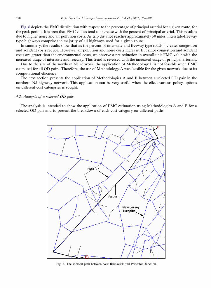
4.2. Analysis of a selected OD pair

The analysis is intended to show the application of FMC estimation using Methodologies A and B for aselected OD pair and to present the breakdown of each cost category on different paths.

Fig. 7. The shortest path between New Brunswick and Princeton Junction.


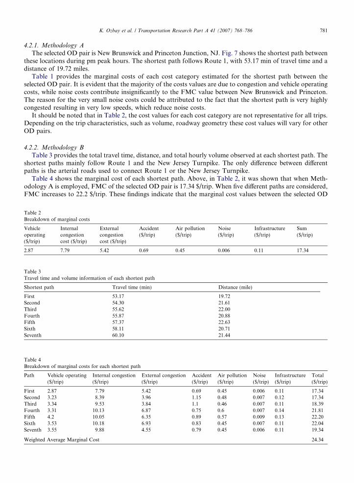
4.2.1. Methodology A

The selected OD pair is New Brunswick and Princeton Junction, NJ. Fig. 7 shows the shortest path betweenthese locations during pm peak hours. The shortest path follows Route 1, with 53.17 min of travel time and adistance of 19.72 miles.

Table 1 provides the marginal costs of each cost category estimated for the shortest path between theselected OD pair. It is evident that the majority of the costs values are due to congestion and vehicle operatingcosts, while noise costs contribute insignificantly to the FMC value between New Brunswick and Princeton.The reason for the very small noise costs could be attributed to the fact that the shortest path is very highlycongested resulting in very low speeds, which reduce noise costs.

It should be noted that in Table 2, the cost values for each cost category are not representative for all trips.Depending on the trip characteristics, such as volume, roadway geometry these cost values will vary for otherOD pairs.

4.2.2. Methodology B

Table 3 provides the total travel time, distance, and total hourly volume observed at each shortest path. Theshortest paths mainly follow Route 1 and the New Jersey Turnpike. The only difference between differentpaths is the arterial roads used to connect Route 1 or the New Jersey Turnpike.

Table 4 shows the marginal cost of each shortest path. Above, in Table 2, it was shown that when Meth-odology A is employed, FMC of the selected OD pair is 17.34 $/trip. When five different paths are considered,FMC increases to 22.2 $/trip. These findings indicate that the marginal cost values between the selected OD

Table 2Breakdown of marginal costs

Vehicleoperating($/trip)

Internalcongestioncost ($/trip)

Externalcongestioncost ($/trip)

Accident($/trip)

Air pollution($/trip)

Noise($/trip)

Infrastructure($/trip)

Sum($/trip)

2.87 7.79 5.42 0.69 0.45 0.006 0.11 17.34

Table 3Travel time and volume information of each shortest path

Shortest path Travel time (min) Distance (mile)

First 53.17 19.72Second 54.30 21.61Third 55.62 22.00Fourth 55.87 20.88Fifth 57.37 22.63Sixth 58.11 20.71Seventh 60.10 21.44

Table 4Breakdown of marginal costs for each shortest path

Path Vehicle operating($/trip)

Internal congestion($/trip)

External congestion($/trip)

Accident($/trip)

Air pollution($/trip)

Noise($/trip)

Infrastructure($/trip)

Total($/trip)

First 2.87 7.79 5.42 0.69 0.45 0.006 0.11 17.34Second 3.23 8.39 3.96 1.15 0.48 0.007 0.12 17.34Third 3.34 9.53 3.84 1.1 0.46 0.007 0.11 18.39Fourth 3.31 10.13 6.87 0.75 0.6 0.007 0.14 21.81Fifth 4.2 10.05 6.35 0.89 0.57 0.009 0.13 22.20Sixth 3.53 10.18 6.93 0.83 0.45 0.007 0.11 22.04Seventh 3.55 9.88 4.55 0.79 0.45 0.006 0.11 19.34

Weighted Average Marginal Cost 24.34


pair are different for different paths and that none of the cost category follows a particular pattern with respectto a certain path. The reason behind different cost values for different paths is, most probably, due to the factthat shortest paths are determined solely on the basis of travel times on each path.

So far, all the analysis regarding the northern NJ network is performed using a static transportation modelloaded by the TP+TM software output. As mentioned above, such tools are inefficient in understanding theeffect of additional demand on the overall performance of the network.

The next section presents the use of microscopic simulation tools in capturing the dynamic nature of trafficnetworks.

5. Estimation of FMC using microscopic simulation

Commonly used transportation-models make use of static traffic assignment to evaluate the impact of var-ious operational changes on highway travel costs. By and large, they do not consider the time-dependentdynamics of traffic flow and demand. Thus, the effects of various operational changes in terms of their impacton traffic congestion have to be modeled using a traffic simulation model, which is the most accurate way tocapture the dynamic nature of traffic flow and demand within a certain time interval.

Once the impact of the operational changes on the traffic flow is captured, the related costs can be calcu-lated using the cost functions presented in Section 3. This methodology, which combines sound economic the-ory with the output of a highly detailed simulation model, is capable to accurately estimate the costs/benefitsof various operational alternatives. In this section, we estimate the costs changes of additional demand, usingPARAMICS simulation software.

5.1. Hypothetical study network

Consider urban highway network as is shown in Fig. 8. OD zones are depicted by the squares. The bold lineindicates the main roadway, whereas the rest are local roadways. During peak hour major demand is fromzone 1 to zone 2 as shown in Table 5. The roadway that connects zone 3 and 4 has priority over the intersect-ing minor roads. Locations of signalized and un-signalized intersections are shown in the legend. Note that thelinks on the main route between the OD pair (1,2) are two-lane roadways, and all other links are one-laneroadways.

The PARAMICS simulation software has the capability of microscopically modeling vehicle-following andlane-changing behavior of individual vehicles.10 The following section shows the application of the simulationmethodology to estimate the FMC cost between the OD pair (1,2), before and after increase in demand. Thispair is selected due to the high hourly traffic demand.

5.2. Analysis

The simulation model of the study network shown in Fig. 8 is simulated for one-hour. Table 6 shows thenetwork performance measures for peak and off-peak periods obtained from the simulation outputs. Note thatthe results are given in a 90% Confidence Interval (C.I.) based on multiple simulation runs.

It is assumed that additional demand between a given OD pair disturbs the network equilibrium. Therefore,to estimate the FMC, the following steps are performed:

• The total demand between the given OD pair is assigned to the network.• Total network cost for the ‘‘before’’ the change is estimated on the basis of the resulting travel times and

traffic flows obtained from the simulation.• Demand between the selected OD pair is increased by an additional unit of demand.

10 PARAMICS allows users to customize many features of the underlying simulation model through Application Programming Interface(API). Users can modify the default simulation routine and test their own models, and obtain detailed outputs using PARAMICS API.

Fig. 8. A hypothetical urban network.

Table 5Origin destination demand matrix (vehicle/h)

O/D 1 2 3 4 5 6 7 8 9 10 11 12

1 0 1025 32 14 15 7 4 20 19 21 10 52 200 0 0 0 0 0 0 0 0 0 0 03 0 0 0 0 0 0 0 122 0 0 0 04 0 48 0 0 0 0 0 0 0 0 0 05 0 72 0 0 0 0 0 0 0 0 0 06 0 66 0 0 0 0 0 0 9 21 88 07 0 32 0 0 0 0 0 0 0 0 0 08 0 0 105 0 0 0 0 0 0 0 0 09 13 41 0 72 5 7 11 11 0 0 0 010 16 10 13 21 29 8 13 13 0 0 0 011 20 93 23 21 21 105 7 13 0 0 0 012 0 31 0 8 37 14 49 0 0 0 0 0

Table 6Network performance – simulation results

Average network travel time (min) Average speed (mph)

Peak period Average 3.8, C.I. [3.4, 4.3] Average 19.5, C.I. [17.4, 21.6]Off-peak Average 2.3, C.I. [2.2, 2.3] Average 27.5, C.I. [27.4, 27.6]


• This increased OD demand is reassigned to the network, and total network cost for the after condition isestimated using the new travel times and travel flows.


• FMC is estimated by calculating the total cost difference between the two networks and dividing by theextra OD demand added to the network.

This methodology can be represented as follows:

TableFMC

TC1

TC2

FMC

TableFMC

TC1

TC2

FMC

FMC ¼ TC2 � TC1

Dð5Þ

where

TC1 total network cost before the additional demand between the OD pair ($)TC2 total network cost after the additional demand between the OD pair ($)D the additional demand included to the network (vehicles/hour)FMC full marginal cost of the selected OD pair ($)

Let us now suppose that the demand between the OD pair (1,2) is increased by D = 100 veh/h to 1725 veh/h. The change in the total network cost would yield the straight-line approximation of the FMC. Table 7 givesthe hourly costs of the network before and after the demand increase, and the respective marginal costs. Itshould be noted that accident costs are not included in the total cost due to the fact that the accident costfunctions presented in Section 3 are route based functions. The use of these functions for each link would over-estimate the accident costs. Based on Eq. (4), the FMC can be calculated as (2844.7 � 2242.0)/100 = $6.02/trip/h.

Table 7 shows that total cost has increased by about 27% (from 2242.2 to 2844.7), and the major increase isobserved at the congestion cost category. The simulation output analysis show that the average mean speed isreduced from 19.5 mph to 13.6 mph by the increase in demand between the OD pair (1,2). The reduction innoise cost can be attributed to the reduction in average speed of vehicles in the network.

Let us now estimate the FMC between the OD pair (1, 2) using Methodology C as described in Section 4.For this purpose, the study network in Fig. 8 is modeled using TransCAD planning software. The traffic flowat each link is assigned based on user-equilibrium traffic assignment, using the OD demand values given inTable 5. Then, the additional demand of D = 100 is introduced between the OD pair (1, 2). Total network costsare estimated for both scenarios. The FMC between the OD pair (1, 2) is calculated based on Eq. (4). Table 8presents the FMC breakdown for each cost category.

Comparing the marginal cost values presented in Tables 7 and 8, it can be observed that there are signif-icant differences in the marginal cost estimations, especially in the congestion cost category when using thestatic planning model’s outputs and the simulation software’s detailed outputs. In the later case total networkcost has increased by only 10.3% (from 1273.2 to 1404.9). As mentioned before, static traffic planning toolssuch as TransCAD do not account for various network or driver related parameters. The use of aggregateoutputs can result in erroneous estimation of the impacts of various operational changes on FMC values.

7Estimation of the OD pair (1,2) using PARAMICS Output ($/h)

Vehicle operating Congestion Infrastructure Air pollution Noise Total

145.7 1729.5 243.6 78.9 44.7 2242.2188.9 2258.6 273.2 87.4 36.6 2844.70.434 5.291 0.296 0.084 �0.081 6.02

8estimation of the OD pair (1,2) using TransCAD output ($/h)

Vehicle operating Congestion Infrastructure Air pollution Noise Total

79.2 947.5 167.8 56.7 22.0 1273.283.5 998.5 176.0 59.7 25.1 1404.90.043 0.51 0.082 0.03 0.031 1.317


6. Summary and conclusions

Accurate estimation of FMC is essential in evaluating various policy and operational changes in highwaytransportation networks. This study is stemmed from the uncertainty of how to estimate the FMC of highwaynetworks with multiple OD pairs and multiple routes. This issue is addressed in Section 4. Three methodol-ogies are presented to estimate the FMC.

The first methodology is due to Ozbay et al. (2001), where the authors selected the shortest route betweeneach selected OD pair, and assumed that the additional demand do not disturb the network equilibrium. Thekey findings of this study are presented in Section 4.1.

The second methodology is to determine several paths (including the shortest path) between each selectedOD pairs, and determine the FMC as the weighted marginal costs of these paths. A simple application of thismethodology is presented in Section 4.2 between two selected cities in NJ using the same northern NJ highwaynetwork as used by Ozbay et al. (2001). It is observed that the marginal values of different paths vary as muchas 28%.

The third methodology assumes that the additional demand disturbs the network equilibrium. It determinesthe FMC by reassigning the network flows due to the additional demand between an OD pair. The differencebetween the total costs of the network before and after the additional demand is calculated to estimate theFMC of the network.

An important contribution of this paper is the application of microscopic simulation software for the FMCestimation process, as presented in Section 5. A hypothetical study network is modeled in PARAMICS microsimulation software. The results of the FMC estimation of a selected OD pair are presented in Table 7. Thevehicle-by-vehicle output data collection capability of PARAMICS enables us to collect detailed travel time,speed, traffic volume data, etc. from the simulation model. The use of a high fidelity traffic simulation modelcan better capture the dynamic nature of traffic flow than a static traffic model. In order to compare the FMCestimation results of a static network tool and a micro simulation tool, the study network is modeled in Trans-CAD. The FMC between the selected OD pair is estimated based on the link flows obtained from TransCAD.The results show substantial differences in the FMC estimation as shown in Table 8.

Furthermore, the use of a powerful micro simulation software, such as PARAMICS, is very efficient inunderstanding and estimating the impact of various operational alternatives to ease congestion, such as capac-ity expansion between a selected OD pair (see Ozbay et al., 2005), the use of intelligent transportation systems,incident management policies (Ozbay and Bartin, 2004), etc.

References

AAA, Your Driving Costs 2003, American Automobile Association (www.ouraaa.com), 2003. Based on Runzheimer International data.Churchill, A., 1972. Road user charges in Central America. In: Silcock, T.H., Bowen, Ian (Eds.), World Bank Staff Occasional Papers.

John Hopkins University Press, Baltimore.Cipriani, R., Porter, M.J., Conroy, N., Johnson, L., Semple, K., 1998. The Full Costs of Transportation in the Central Puget Sound region

in 1995. TRB Preprint: 980670, Transportation Board 77th Annual meeting, Washington, DC.Delucchi, M., Hsu, S., 1998. The external damage cost of noise emitted from motor vehicles. Journal of Transportation and Statistics 1, 1–

24.Environmental Protection Agency Publications, 1995. National Emission Trends.Federal Highway Administration (FHWA). Motor Vehicle Accident Costs, 2005, Available online: <http://www.fhwa.dot.gov/legsregs/

directives/techadvs/t75702>.Kelly Blue Book Website, 2006. Available from: <http://www.kbb.com/>.Levinson, D.M., Gillen, D., 1998. The full cost of intercity highway transportation. TRB Preprint: 980263, Transportation Research

Board 77th Annual meeting, Washington, DC.Levinson, D., Gillen, D., Kanafani, A., Mathieu, J.M., 1996. The full cost of intercity transportation – a comparison of high speed rail, air,

and highway transportation in California. UCB-IS-RR-96-3, Berkeley, CA, Institute of Transportation Studies, University ofCalifornia at Berkeley.

Link, H., 2006. An econometric analysis of motorway renewal costs in Germany. Transportation Research Part A 40, 19–34.Mayeres, I., Ochelen, S., Proost, S., 1996. The marginal external costs of urban transport. Transportation Research D 1 (2), 111–130.Mun, Se-IL., 1994. Traffic jams and congestion tolls. Transportation Research B 28, 365–375.Nelson, J.P., 1982. Highway noise and property values: a survey of recent evidence. Journal of Transport Economics and Policy,

117–138.

http://www.ouraaa.com

http://www.fhwa.dot.gov/legsregs/directives/techadvs/t75702

http://www.fhwa.dot.gov/legsregs/directives/techadvs/t75702

http://www.kbb.com/


US Department of Transportation. Crash Records, 2005, Available from: <http://www.state.nj.us/transportation/refdata/accident/rawdata01-03.shtm>.

Ozbay, K., Bartin, B., 2004. Estimation of economic impact of V.M.S. route guidance using micro simulation. In: Economic Impacts ofIntelligent Transportation Systems: Innovations and Case Studies. Research in Transportation Economics, vol. 8, pp. 211–238(Chapter 11).

Ozbay, K., Bartin, B.O., Berechman, J., 2000. Full costs of highway transportation in New Jersey, New Jersey Department ofTransportation Report.

Ozbay, K., Bartin, B., Berechman, J., 2001. Estimation and evaluation of full marginal costs of highway transportation in New Jersey.Journal of Transportation and Statistics 4 (1).

Ozbay, K., Yanmaz-Tuzel, O., Mudigonda, S., Bartin, B., Berechman, J., 2005. ‘‘Cost of transporting people in New Jersey-Phase II’’,New Jersey Department of Transportation Draft Report.

Peat Marwick Stevenson & Kellog (PMSK), 1993. The cost of transporting people in the British Columbia mainland. Transport 2021Technical Report 11.

Small, K., Chu, X., 2003. Hypercongestion. Journal of Transport Economics and Policy 37, 319–352.US Department of Transportation, 1999. Cost of Owning and Operating Automobiles, Vans and Light Trucks.Vickrey, W., 1968. Automobile accidents, tort law, externalities, and insurance: an economists critique. Law and Contemporary Problems

33, 464–487.

http://www.state.nj.us/transportation/refdata/accident/rawdata01-03.shtm

http://www.state.nj.us/transportation/refdata/accident/rawdata01-03.shtm

alternative methods for estimating full marginal costs of highway transportation

Documents