almost-inner derivations of lie algebras · this master thesis is about almost-inner derivations of...
TRANSCRIPT
FACULTY OF SCIENCE
Almost-inner derivationsof Lie algebras
Bert VERBEKE
Supervisor: Prof. dr. K. DekimpeCo-supervisor: Prof. dr. D. BurdeAffiliation (Universitat Wien)
Thesis presented in
fulfillment of the requirements
for the degree of Master of Science
in Mathematics
Academic year 2015-2016
© Copyright by KU Leuven
Without written permission of the promotors and the authors it is forbidden to repro-duce or adapt in any form or by any means any part of this publication. Requests forobtaining the right to reproduce or utilize parts of this publication should be addressedto KU Leuven, Faculteit Wetenschappen, Geel Huis, Kasteelpark Arenberg 11 bus 2100,3001 Leuven (Heverlee), Telephone +32 16 32 14 01.
A written permission of the promotor is also required to use the methods, products,schematics and programs described in this work for industrial or commercial use, and forsubmitting this publication in scientific contests.
Preface
This master thesis is about almost-inner derivations of Lie algebras, written to filfill therequirements for becoming a Master of Science in Mathematics. I started studying thesubject in September 2015. The process of researching and writing this thesis took metill the start of June 2016. During this period, there are a lot of people who helped memaking this thesis. I want to thank them for their help and support.
I would first like to express my gratitude to Prof. dr. Karel Dekimpe, for giving mealready the taste of doing research, for the excellent guidance, for reading all preliminaryversions and giving advice and comments to improve this thesis. Thank you for alwaysmaking time to help, both in Leuven and in Kortrijk. I could not have imagined havinga better promotor.
During the first semester, I stayed in Vienna, where I constantly could count on the aidof my co-supervisor Prof. Dietrich Burde. Thank you for answering my questions, forcomparing results and for increasing my language skills.
Further, I would like to acknowledge Prof. dr. Nero Budur and dr. Jonas Dere for readingand evaluating this master thesis.
I also want to thank my friends for the many moments of recreation. In particular, Iwould like to express my gratitude to my fellow mathematicians of the Kulak for thepleasant past five years.
Last but not the least, I would like to thank my parents, sister, brother and brother-in-lawfor encouraging me in all of my pursuits and for providing me with constant support.
Bert Verbeke
Heule, June 2, 2016
i
Abstract
The purpose of this thesis is to study almost-inner derivations of Lie algebras in an al-gebraic way. An almost-inner derivation ϕ of a Lie algebra g is a derivation ϕ such thatϕ(X) ∈ [X,g] for all X ∈ g. This kind of derivations arises in the study of spectral ge-ometry, in particular in the construction of isospectral and non-isometric manifolds. Thenotion has not been much studied algebraically and only in some specific cases.
In the first chapter, the geometric connection between Lie groups and Lie algebras isexplained. Further, there is an algebraic introduction to Lie algebra-theory. Those pre-liminaries will be useful in the following chapters.
The second chapter is devoted to the concept of almost-inner derivations. First, somespecial types of derivations are introduced. This concerns in particular the almost-innerones, which form a generalisation of the inner derivations. These notions permit to un-derstand the underlying geometric motivation, which is worked out in the second section.It illustrates why almost-inner derivations are interesting to study. To investigate theconcept more thoroughly, there is need of some theory concerning the definition. This iselaborated in the last section. There is a procedure to compute the set of all almost-innerderivations. This working method is explained and illustrated with an example. It is usedas a manual for the calculations in the rest of the thesis.
In the third chapter, special classes of Lie algebras are introduced. The first class consistsof the complex Lie algebras of dimension at most four. Next, the metabelian filiformLie algebras are studied. The following class concerns two-step nilpotent Lie algebraswhich are defined by graphs. Further, also free nilpotent Lie algebras and Lie algebrasof strictly uppertriangular and uppertriangular matrices are treated. For these classes(and sometimes only for specific cases), the set of all almost-inner derivations is com-puted. For the metabelian filiform Lie algebras, it turns out that the dimension of theset of almost-inner derivations is at most one more than the dimension of the set of innerderivations. In all other cases, both sets are equal. The question for the free nilpotent Liealgebras is only solved when the nilindex is two or three. In the context of almost-innerderivations, nilpotent Lie algebras are geometrically of most importance. Therefore, theintroduced classes (except for the first and last ones) only consist of nilpotent Lie algebras.
The appendix contains some computer programs implemented in Matlab. Those algo-rithms ease the computations. The first part checks whether or not given structure con-stants define a Lie algebra. The second section concerns algorithms computing a basis forthe space of all derivations of a given Lie algebra.
ii
Samenvatting
In deze thesis worden bijna-inwendige derivaties van Lie algebra’s bestudeerd op een al-gebraısche manier. Een bijna-inwendige derivatie ϕ van een Lie algebra g is een derivatieϕ zodat ϕ(X) ∈ [X,g] voor alle X ∈ g. Dit soort derivaties duikt op in de spec-trale meetkunde, in het bijzonder bij de constructie van isospectrale en niet-isometrischevarieteiten. De bijna-inwendige derivaties zijn nog niet vaak algebraısch bestudeerd enenkel in bepaalde specifieke gevallen.
In het eerste hoofdstuk wordt het meetkundig verband tussen Lie groepen en Lie alge-bra’s uitgewerkt. Verder is er ook een algebraısche inleiding op Lie algebra-theorie. Deingevoerde concepten zullen in de latere hoofdstukken terugkomen.
Het tweede hoofdstuk handelt over bijna-inwendige derivaties. Eerst worden verschillendesoorten derivaties ingevoerd. In het bijzonder zijn dat de bijna-inwendige derivaties, eenveralgemening van de inwendige derivaties. Deze noties laten het toe om de achterliggendemeetkundige motivatie te begrijpen. De tweede sectie illustreert waarom bijna-inwendigederivaties interessant zijn om onderzoek naar te doen. Om deze concepten verder tekunnen bestuderen, is er meer theorie nodig. Dit is uitgewerkt in het laatste deel. Hetberekenen van de verzameling van alle bijna-inwendige derivaties gebeurt aan de handvan een vast stappenplan. Deze werkwijze is uitgelegd en geıllustreerd aan de hand vaneen voorbeeld. Het vormt de leidraad bij de berekeningen in de rest van de thesis.
In het derde hoofdstuk worden speciale klassen van Lie algebra’s ingevoerd. Het eerstetype bestaat uit de complexe Lie algebra’s waarvan de dimensie hoogstens vier is. Ver-volgens worden meta-abelse filiforme Lie algebra’s bestudeerd. De derde klasse bevat detwee-staps nilpotente Lie algebra’s die door grafen gedefinieerd zijn. Ook worden de vrijenilpotente Lie algebra’s en de (strikte) bovendriehoeksmatrices behandeld. Voor al dezeklassen (in sommige gevallen enkel voor specifieke voorbeelden) is de verzameling vanbijna-inwendige derivaties berekend. Voor de meta-abelse filiforme Lie algebra’s blijktdat de dimensie van de verzameling bijna-inwendige derivaties hoogstens een meer is dande dimensie van de verzameling inwendige derivaties. In alle andere gevallen zijn beideverzamelingen gelijk. Voor de vrije nilpotente Lie algebra’s is het resultaat enkel gekendals de nilindex gelijk is aan twee of drie. In de context van bijna-inwendige Lie algebra’szijn de nilpotente Lie algebra’s meetkundig het meest van belang. Daarom bestaan deingevoerde klassen (op de eerste en laatste na) enkel uit nilpotente Lie algebra’s.
De appendix bevat een aantal computerprogramma’s die geımplementeerd zijn in Matlab.Deze algoritmes maken de berekeningen eenvoudiger. In het eerste deel wordt nagegaan
iii
iv
of gegeven structuurconstanten al dan niet een Lie algebra definieren. Het volgende deelgaat over algoritmes die een basis berekenen voor de verzameling van derivaties voor eengegeven Lie algebra.
Contents
Preface i
Abstract ii
Samenvatting iii
1 Basic theory of Lie algebras 11.1 Lie groups and Lie algebras . . . . . . . . . . . . . . . . . . . . . . . . . . . . 11.2 Basic theory of Lie algebras . . . . . . . . . . . . . . . . . . . . . . . . . . . . 3
1.2.1 Definitions . . . . . . . . . . . . . . . . . . . . . . . . . . . . . . . . . . 31.2.2 Special constructions of Lie algebras . . . . . . . . . . . . . . . . . . . 8
2 Almost-inner derivations 112.1 Definitions . . . . . . . . . . . . . . . . . . . . . . . . . . . . . . . . . . . . . . . 112.2 Geometric motivation . . . . . . . . . . . . . . . . . . . . . . . . . . . . . . . . 16
2.2.1 Isospectral manifolds . . . . . . . . . . . . . . . . . . . . . . . . . . . . 162.2.2 Nilmanifolds . . . . . . . . . . . . . . . . . . . . . . . . . . . . . . . . . 172.2.3 Automorphisms . . . . . . . . . . . . . . . . . . . . . . . . . . . . . . . 19
2.3 First considerations . . . . . . . . . . . . . . . . . . . . . . . . . . . . . . . . . 202.3.1 Conditions on the parameters of an almost-inner derivation . . . . . 212.3.2 Properties to compute the almost-inner derivations . . . . . . . . . . 26
3 Different classes of Lie algebras 323.1 Low-dimensional Lie algebras . . . . . . . . . . . . . . . . . . . . . . . . . . . 323.2 Filiform Lie algebras . . . . . . . . . . . . . . . . . . . . . . . . . . . . . . . . . 363.3 Two-step nilpotent Lie algebras determined by graphs . . . . . . . . . . . . 473.4 Free nilpotent Lie algebras . . . . . . . . . . . . . . . . . . . . . . . . . . . . . 49
3.4.1 Free nilpotent Lie algebras with nilindex two . . . . . . . . . . . . . . 533.4.2 Free nilpotent Lie algebras with nilindex three . . . . . . . . . . . . . 53
3.5 Triangular matrices . . . . . . . . . . . . . . . . . . . . . . . . . . . . . . . . . 573.5.1 Strictly uppertriangular matrices . . . . . . . . . . . . . . . . . . . . . 583.5.2 Uppertriangular matrices . . . . . . . . . . . . . . . . . . . . . . . . . 62
Conclusion 69
A Algorithms 71A.1 Check of the Jacobi identity . . . . . . . . . . . . . . . . . . . . . . . . . . . . 71A.2 Computation of a basis for Der(g) . . . . . . . . . . . . . . . . . . . . . . . . 72
v
Chapter 1
Basic theory of Lie algebras
This chapter introduces the basic theory of Lie algebras which will be used in later chap-ters. First, the geometric connection between Lie groups and Lie algebras is explained.Then, there is an algebraic introduction to Lie algebras. This contains some well-knownexamples and terminology of Lie algebras. Those preliminaries are important for the restof this thesis.
1.1 Lie groups and Lie algebras
In this section, the concepts of a Lie group and a Lie algebra are introduced. Lie groupsare important for geometrical purposes, but Lie algebras are easier to handle for manycomputations. Therefore, to gain insight about Lie groups, the corresponding Lie algebrasare studied. The material in this section is based on [4].
Definition 1.1.1 (Lie group). A (real) Lie group G is a group which is a smooth manifoldand for which the multiplication µ and inversion ν are smooth maps.
In this definition, the maps µ ∶ G ×G → G ∶ (x, y) ↦ xy and ν ∶ G → G ∶ x ↦ x−1 aredefined as expected.
Example 1.1.2. Denote Mn(R) the space of all real (n×n)-matrices. Consider this spaceas Rn2
. The determinant function det ∶ Rn2 → R ∶ A ↦ det(A) is a smooth map. Hence,the general linear group
GL(n,R) ∶= {A ∈Mn(R) ∣ det(A) ≠ 0}
is open in Rn2and therefore a manifold. Further, GL(n,R) is obviously a group. More-
over, the entries of the product of two matrices are polynomials in the entries of the twomatrices. Therefore, the matrix multiplication and inversion are smooth maps, whichmeans that GL(n,R) defines a Lie group.
The left translation is the following notion to be defined.
Definition 1.1.3 (Left translation). Let G be a Lie group and g ∈ G. The left translationλg ∶ G→ G is defined by λg(h) = µ(g, h) = gh.
1
CHAPTER 1. BASIC THEORY OF LIE ALGEBRAS 2
Since the multiplication map of a Lie group is smooth by definition, λg defines adiffeomorphism for the manifold G, where the inverse is given by λg−1 .
Let f ∶ M → N be a smooth map between two smooth manifolds M and N . Thedifferential of f at x is denoted by dfx ∶ TxM → Tf(x)N . Let X ∈ TeG and g ∈ G, thenLX(g) is defined as d(λg)e(X) ∈ TgG. It is thus the differential of the left translation inthe neutral element. The map LX ∶ G→ TG is a vector field on G, since LX(g) ∈ TgG andLX is smooth.
The notion X(M) is used for the set of all smooth vector fields on the manifold M .For arbitrary vector fields on a smooth manifold, the Lie bracket can be defined.
Definition 1.1.4 (Lie bracket). Let M be a smooth manifold and let ξ, η ∈ X(M) bevector fields. The Lie bracket [ξ, η] ∈ X(M) of ξ and η is the unique vector field for which[ξ, η] ⋅ f = ξ ⋅ (η ⋅ f) − η ⋅ (ξ ⋅ f) holds for all smooth functions f ∶M → R.
It is clear that the Lie bracket is bilinear and skew-symmetric.Let M be a smooth manifold and let ξ, η and ζ ∈ X(M) be vector fields on M . By
calculation, it is easy to show that the Jacobi-identity
[ξ, [η, ζ]] + [η, [ζ, ξ]] + [ζ, [ξ, η]] = 0
holds. Another well-known concept in differential geometry is that of the pullback.
Definition 1.1.5 (Pullback). Let f ∶M → N be a local diffeomorphism for manifolds Mand N and let ξ ∈ X(N) be a vector field on N . The pullback f∗ξ ∈ X(M) is defined by
f∗ξ(x) ∶= (dfx)−1 ○ ξ(f(x)) for all x ∈M.
Let G be a Lie group with g ∈ G and let ξ ∈ X(G) be a vector field, then (λg)∗ξ ∈ X(G).A vector field is called left invariant if it is preserved by the pullback of the left translationby g, where g is an arbitrary element of the Lie group.
Definition 1.1.6 (Left invariant vector field). Let G be a Lie group and let ξ ∈ X(G).Then ξ is left invariant if and only if (λg)∗ξ = ξ for all g ∈ G.
The space of left invariant vector fields of a Lie group G is denoted by XL(G). Nextproposition reveals a relation between the tangent space at the neutral element and theset of all left invariant vector fields of a Lie group.
Proposition 1.1.7. Let G be a Lie group and denote g = TeG. The vector field LX is leftinvariant, where X ∈ g. Moreover, g is isomorphic with XL(G).
Proof. Let g, h ∈ G be arbitrary and X ∈ g. By definition,
((λg)∗LX)(h) = (d(λg)h)−1 ○LX(λg(h)) = d(λg−1)gh ○ d(λgh)e(X) = d(λh)e(X) = LX(h)holds, which means that LX is left invariant. Hence, there are linear maps between g andXL(G). Define
ϕ ∶ g→ XL(G) ∶X ↦ LX and ψ ∶ XL(G)→ g ∶ ξ ↦ ξ(e).By definition, LX(e) = X, such that ψ ○ ϕ = Idg. On the other hand, if ξ ∈ XL(G) andX = ξ(e), then
ξ(g) = ((λg−1)∗ξ)(g) = (d(λg−1)g)−1○ξ(λg−1(g)) = d(λg)e○ξ(g−1g) = d(λg)e(X) = LX(g)is satisfied. This means that ξ = LX and ϕ○ψ is the identity on XL(G). Hence, the linearmaps ϕ and ψ are inverse linear isomorphisms between g and XL(G).
CHAPTER 1. BASIC THEORY OF LIE ALGEBRAS 3
It is easy to check that for every local diffeomorphism f ∶ M → N (where M and Nare manifolds), the equality [f∗ξ, f∗η] = f∗([ξ, η]) holds for all ξ, η ∈ X(N). In particular,let G be a Lie group with g ∈ G and let ξ, η ∈ XL(G) be left invariant vector fields, then
λ∗g[ξ, η] = [λ∗gξ, λ∗gη] = [ξ, η]
holds, which means that [ξ, η] ∈ XL(G).
Definition 1.1.8 (Lie algebra). Let G be a Lie group. The Lie algebra of G is the tangentspace g = TeG with the map
[, ] ∶ g × g→ g ∶ (X,Y )↦ [X,Y ] = [LX , LY ](e).
Due to the last proposition, this is well-defined and [LX , LY ] = L[X,Y ] holds. In thisdefinition, the Lie bracket is skew-symmetric and satisfies the Jacobi-identity, since theseare properties of the Lie bracket of vector fields. Next example gives the Lie algebra ofthe general linear group.
Example 1.1.9. Denote the Lie algebra of GL(n,R) with gl(n,R). It is clear that, as avector space, gl(n,R) = Mn(R). Let A ∈ GL(n,R) and B ∈ Mn(R). One can show thatthe Lie bracket on gl(n,R) is given by
[A,B] = [LA, LB](e) = AB −BA,
for all A,B ∈Mn(R).
For the rest of this thesis, the Lie algebras will be studied algebraically instead ofgeometrically.
1.2 Basic theory of Lie algebras
As showed in the first section, Lie algebras can be defined as the tangent space at theneutral element of a Lie group. So, for every Lie group, there is a corresponding Liealgebra. In his third fundamental theorem, Lie showed that the converse is also true forfinite-dimensional real Lie algebras. However, it is also interesting to study Lie algebraswithout the underlying Lie group. In this section, an algebraic definition of a Lie algebrais given. The notion has the same properties as before, but makes it possible to workwithout the background from differential geometry. Since the Lie groups from Section1.1 were real manifolds, the corresponding Lie algebras were real too. However, there isno need to restrict to the case where K = R. The same reasoning as before can be donesimilarly for other fields. When the field is not denoted, the result holds for arbitraryfields.
1.2.1 Definitions
This section elaborates the terminology which will be used in later chapters. First, thedefinition of an algebra is recalled.
Definition 1.2.1 (Algebra). Let K be a field. An algebra over a field K is a K-vectorspace A together with a bilinear map ⋅ ∶ A ×A→ A.
CHAPTER 1. BASIC THEORY OF LIE ALGEBRAS 4
A Lie algebra is an algebra, for which the bilinear map is called the Lie bracket. Thisbracket satisfies certain conditions, motivated by the corresponding properties of the Liebracket for vector fields.
Definition 1.2.2 (Lie algebra). Let K be a field. A Lie algebra g over K is an algebrawhere the bilinear map
g × g→ g ∶ (X,Y )↦ [X,Y ]satisfies the following properties:
• The bracket [X,X] = 0 holds for all X ∈ g;
• For all X,Y and Z ∈ g, the Jacobi identity [X, [Y,Z]]+ [Y, [Z,X]]+ [Z, [X,Y ]] = 0is fulfilled.
The first condition implies skew-symmetry, since for all X,Y ∈ g
0 = [X + Y,X + Y ] = [X,X] + [X,Y ] + [Y,X] + [Y,Y ] = [X,Y ] + [Y,X]
holds by bilinearity of the bracket. When char(K) ≠ 2, both concepts are even equivalent.Since a Lie algebra is a vector space, every element can be expressed uniquely as linear
combination of the basis vectors. Although a Lie algebra can have infinite dimension, onlyfinite-dimensional Lie algebras are studied in this thesis.
Definition 1.2.3 (Structure constants). Let g be an n-dimensional Lie algebra with basisB = {X1,X2, . . . ,Xn}. Then there exist ckij ∈K such that
[Xi,Xj] =n
∑k=1
ckijXk.
These values ckij (with 1 ≤ i, j, k ≤ n) are the structure constants of g with respect to thebasis B.
The conditions imposed on the structure constants by the Jacobi identity can be cal-culated as follows. Consider an n-dimensional Lie algebra g with basis B = {X1, . . . ,Xn}.Let Xi,Xj and Xk be three arbitrary basis vectors, so 1 ≤ i, j, k ≤ n. Then
0 = [Xi, [Xj,Xk]] + [Xj, [Xk,Xi]] + [Xk, [Xi,Xj]]
=n
∑m=1
cmjk[Xi,Xm] +n
∑m=1
cmki[Xj,Xm] +n
∑m=1
cmij [Xk,Xm]
=n
∑m=1
(cmjk[Xi,Xm] + cmki[Xj,Xm] + cmij [Xk,Xm])
=n
∑m=1
(cmjkn
∑l=1
climXl + cmkin
∑l=1
cljmXl + cmijn
∑l=1
clkmXl)
=n
∑m=1
n
∑l=1
(cmjkclim + cmkicljm + cmij clkm)Xl
holds. This means thatn
∑m=1
(cmjkclim + cmkicljm + cmij clkm) = 0 (1.1)
CHAPTER 1. BASIC THEORY OF LIE ALGEBRAS 5
has to be satisfied for all 1 ≤ i, j, k, l ≤ n.It suffices to specify the Lie bracket [Xi,Xj] and hence the structure constants only
when i < j, since [Xi,Xi] = 0 and [Xj,Xi] = −[Xi,Xj]. Usually, only the non-vanishingbrackets are mentioned. It can be examined whether or not an algebra with given structureconstants defines a Lie algebra, by verifying the equations (1.1) for all possible values. Inappendix A.1, algorithm checkJacobi(C) in Code A.2 checks whether or not C representsa Lie algebra. The input is an (n×n×n)-matrix C where C(i, j, k) stands for the structureconstant ckij. For the convenience, only the non-zero entries C(i, j, k) are implementedwhen i < j.
Definition 1.2.4 (Appearances of a basis vector). Let g be an n-dimensional Lie algebrawith basis B = {X1, . . . ,Xn}. A basis vector Xk is said to appear m times if there existexactly m different pairs {i, j} so that ckij = −ckji ≠ 0.
Of course, this definition depends on the choice of the basis.
Example 1.2.5. Let g be the four-dimensional Lie algebra over a field K with char(K) ≠ 0and basis B = {X1,X2,X3,X4} and non-vanishing Lie brackets
[X1,X2] = X2; [X1,X3] = X2 +X3; [X1,X4] = 2X4 and [X2,X3] = X4.
It is not so hard to show that the structure constants satisfy (1.1) for all 1 ≤ i, j, k, l ≤ 4.For this Lie algebra, X1 does not appear, X2 and X4 appear twice and X3 appears once.
An important example of a Lie algebra is the following, motivated by the example ofthe first section.
Example 1.2.6. Let V be a finite-dimensional vector space over a field K. Denote thedimension of V by dim(V ) = n. The set gl(V ) denotes all linear maps from V to V . Thisis a Lie algebra for which the Lie bracket is defined by
[X,Y ] = X ○ Y − Y ○X for all X,Y ∈ gl(V ).
It is easy to verify that the conditions on the Lie bracket are satisfied. Every linearmap from V to V can be represented by an (n × n)-matrix. Therefore, the vector spacegl(n,K) of all (n × n)-matrices also defines a Lie algebra, where the Lie bracket is givenby
[A,B] = AB −BA for all A,B ∈ gl(n,K).Here, AB denotes the usual matrix multiplication. This example will turn up a lot in thisthesis.
The next definition is that of a Lie subalgebra, a vector subspace for which the Liebracket is conserved for all elements.
Definition 1.2.7 (Lie subalgebra). Let g be a Lie algebra. A vector subspace h ⊆ g is aLie subalgebra if [X,Y ] ∈ h for all X,Y ∈ h.
It is clear that a Lie subalgebra is also a Lie algebra.
CHAPTER 1. BASIC THEORY OF LIE ALGEBRAS 6
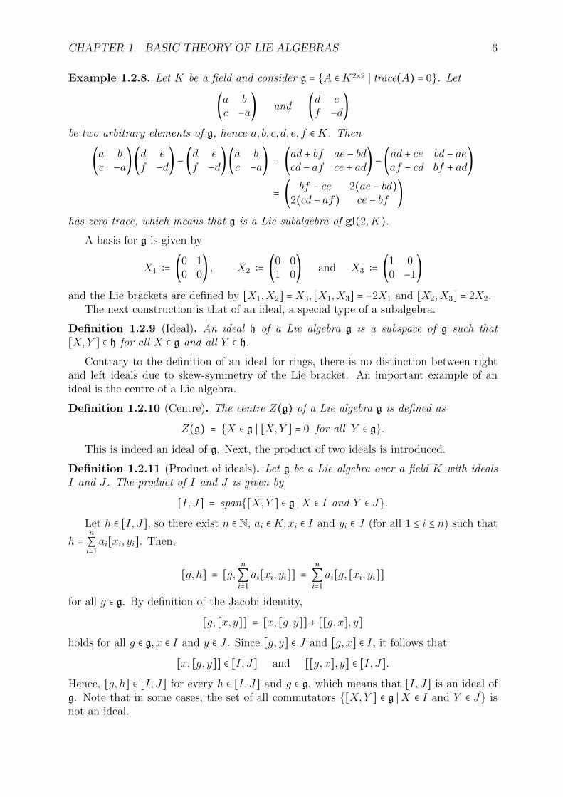
Example 1.2.8. Let K be a field and consider g = {A ∈K2×2 ∣ trace(A) = 0}. Let
(a bc −a) and (d e
f −d)
be two arbitrary elements of g, hence a, b, c, d, e, f ∈K. Then
(a bc −a)(d e
f −d) − (d ef −d)(a b
c −a) = (ad + bf ae − bdcd − af ce + ad) − (ad + ce bd − ae
af − cd bf + ad)
= ( bf − ce 2(ae − bd)2(cd − af) ce − bf )
has zero trace, which means that g is a Lie subalgebra of gl(2,K).
A basis for g is given by
X1 ∶= (0 10 0
) , X2 ∶= (0 01 0
) and X3 ∶= (1 00 −1
)
and the Lie brackets are defined by [X1,X2] =X3, [X1,X3] = −2X1 and [X2,X3] = 2X2.The next construction is that of an ideal, a special type of a subalgebra.
Definition 1.2.9 (Ideal). An ideal h of a Lie algebra g is a subspace of g such that[X,Y ] ∈ h for all X ∈ g and all Y ∈ h.
Contrary to the definition of an ideal for rings, there is no distinction between rightand left ideals due to skew-symmetry of the Lie bracket. An important example of anideal is the centre of a Lie algebra.
Definition 1.2.10 (Centre). The centre Z(g) of a Lie algebra g is defined as
Z(g) = {X ∈ g ∣ [X,Y ] = 0 for all Y ∈ g}.This is indeed an ideal of g. Next, the product of two ideals is introduced.
Definition 1.2.11 (Product of ideals). Let g be a Lie algebra over a field K with idealsI and J . The product of I and J is given by
[I, J] = span{[X,Y ] ∈ g ∣X ∈ I and Y ∈ J}.Let h ∈ [I, J], so there exist n ∈ N, ai ∈K,xi ∈ I and yi ∈ J (for all 1 ≤ i ≤ n) such that
h =n
∑i=1ai[xi, yi]. Then,
[g, h] = [g,n
∑i=1
ai[xi, yi]] =n
∑i=1
ai[g, [xi, yi]]
for all g ∈ g. By definition of the Jacobi identity,
[g, [x, y]] = [x, [g, y]] + [[g, x], y]holds for all g ∈ g, x ∈ I and y ∈ J . Since [g, y] ∈ J and [g, x] ∈ I, it follows that
[x, [g, y]] ∈ [I, J] and [[g, x], y] ∈ [I, J].Hence, [g, h] ∈ [I, J] for every h ∈ [I, J] and g ∈ g, which means that [I, J] is an ideal ofg. Note that in some cases, the set of all commutators {[X,Y ] ∈ g ∣X ∈ I and Y ∈ J} isnot an ideal.
CHAPTER 1. BASIC THEORY OF LIE ALGEBRAS 7
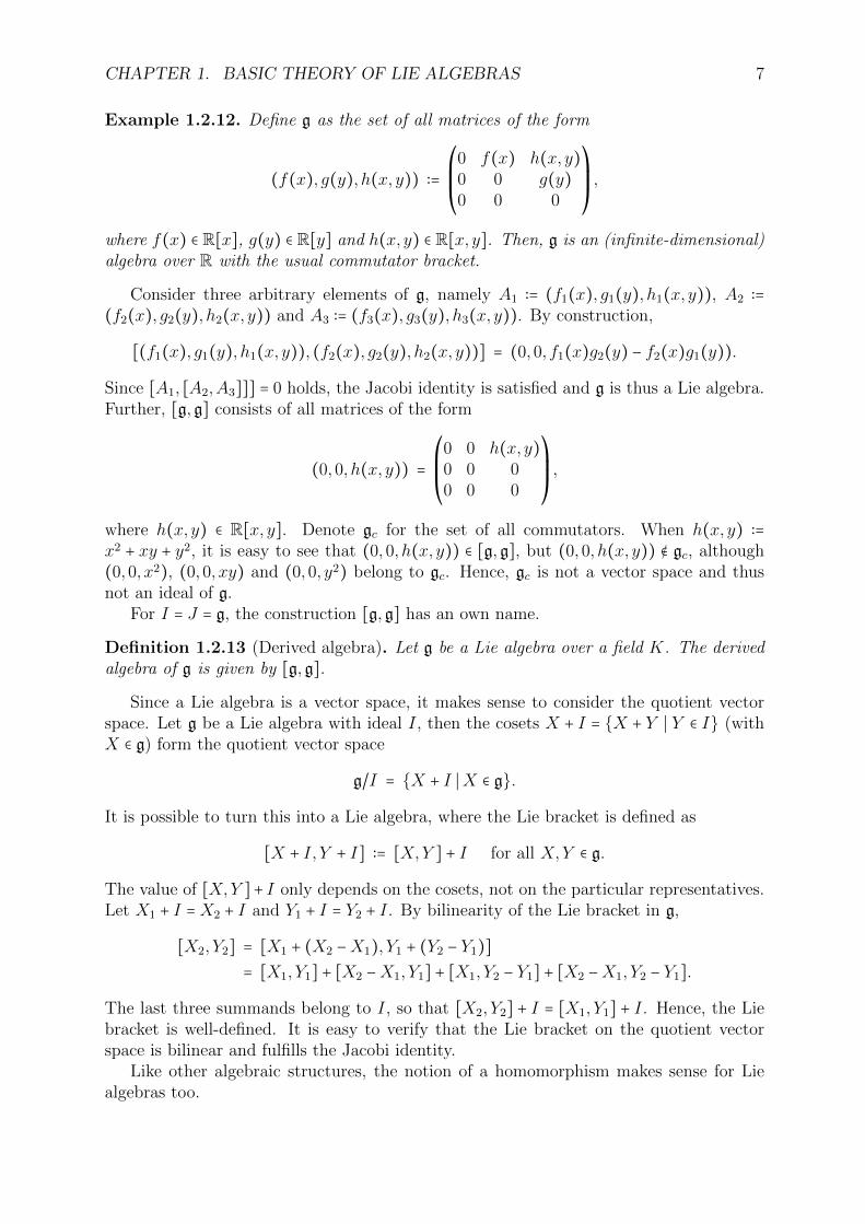
Example 1.2.12. Define g as the set of all matrices of the form
(f(x), g(y), h(x, y)) ∶=⎛⎜⎜⎝
0 f(x) h(x, y)0 0 g(y)0 0 0
⎞⎟⎟⎠,
where f(x) ∈ R[x], g(y) ∈ R[y] and h(x, y) ∈ R[x, y]. Then, g is an (infinite-dimensional)algebra over R with the usual commutator bracket.
Consider three arbitrary elements of g, namely A1 ∶= (f1(x), g1(y), h1(x, y)), A2 ∶=(f2(x), g2(y), h2(x, y)) and A3 ∶= (f3(x), g3(y), h3(x, y)). By construction,
[(f1(x), g1(y), h1(x, y)), (f2(x), g2(y), h2(x, y))] = (0,0, f1(x)g2(y) − f2(x)g1(y)).
Since [A1, [A2,A3]]] = 0 holds, the Jacobi identity is satisfied and g is thus a Lie algebra.Further, [g,g] consists of all matrices of the form
(0,0, h(x, y)) =⎛⎜⎜⎝
0 0 h(x, y)0 0 00 0 0
⎞⎟⎟⎠,
where h(x, y) ∈ R[x, y]. Denote gc for the set of all commutators. When h(x, y) ∶=x2 + xy + y2, it is easy to see that (0,0, h(x, y)) ∈ [g,g], but (0,0, h(x, y)) ∉ gc, although(0,0, x2), (0,0, xy) and (0,0, y2) belong to gc. Hence, gc is not a vector space and thusnot an ideal of g.
For I = J = g, the construction [g,g] has an own name.
Definition 1.2.13 (Derived algebra). Let g be a Lie algebra over a field K. The derivedalgebra of g is given by [g,g].
Since a Lie algebra is a vector space, it makes sense to consider the quotient vectorspace. Let g be a Lie algebra with ideal I, then the cosets X + I = {X + Y ∣ Y ∈ I} (withX ∈ g) form the quotient vector space
g/I = {X + I ∣X ∈ g}.
It is possible to turn this into a Lie algebra, where the Lie bracket is defined as
[X + I, Y + I] ∶= [X,Y ] + I for all X,Y ∈ g.
The value of [X,Y ]+ I only depends on the cosets, not on the particular representatives.Let X1 + I =X2 + I and Y1 + I = Y2 + I. By bilinearity of the Lie bracket in g,
[X2, Y2] = [X1 + (X2 −X1), Y1 + (Y2 − Y1)]= [X1, Y1] + [X2 −X1, Y1] + [X1, Y2 − Y1] + [X2 −X1, Y2 − Y1].
The last three summands belong to I, so that [X2, Y2] + I = [X1, Y1] + I. Hence, the Liebracket is well-defined. It is easy to verify that the Lie bracket on the quotient vectorspace is bilinear and fulfills the Jacobi identity.
Like other algebraic structures, the notion of a homomorphism makes sense for Liealgebras too.
CHAPTER 1. BASIC THEORY OF LIE ALGEBRAS 8
Definition 1.2.14 (Homomorphism). Let g1 and g2 be Lie algebras over the same fieldK. A linear map ϕ ∶ g1 → g2 is a homomorphism if
ϕ([X,Y ]) = [ϕ(X), ϕ(Y )]
holds for all X,Y ∈ g1. A bijective homomorphism is called an isomorphism.
The bracket on the left side is taken in g1 and the bracket on the right side in g2.The following example of a Lie algebra homomorphism will also show up in the next
chapter.
Example 1.2.15. Let g be a Lie algebra over a field K. The adjoint homomorphismad ∶ g→ gl(g) is defined as
(ad(X)) ∶ g→ g ∶ Y ↦ [X,Y ] for all X,Y ∈ g.
Since the Lie bracket is bilinear, ad(X) is linear and belongs hence to gl(g). Moreover,ad is linear for the same reason. Let Z ∈ g be arbitrary. The Jacobi identity
[X, [Y,Z]] + [Y, [Z,X]] + [Z, [X,Y ]] = 0
is equivalent with[[X,Y ], Z] = [X, [Y,Z]] − [Y, [X,Z]].
For all X,Y ∈ g, this means that
ad([X,Y ]) = ad(X) ○ ad(Y ) − ad(Y ) ○ ad(X)= [ad(X),ad(Y )],
where the first bracket is taken in g and the second bracket in gl(g). Hence, the adjointmap is indeed a Lie algebra homomorphism.
The next subsection is devoted to the introduction of some notions. Those conceptshave an important role in Chapter 3 of this thesis, where the almost-inner derivations ofspecial classes of Lie algebras will be computed.
1.2.2 Special constructions of Lie algebras
In the next chapter, almost-inner derivations are defined. This concept is geometricallyimportant, especially for nilpotent Lie algebras. This kind of Lie algebras is introducedin this section. First, the notion of a direct sum of Lie algebras is explained.
Definition 1.2.16 (Direct sum of Lie algebras). Let g1 and g2 be two Lie algebras overthe same field K. The direct sum g = g1 ⊕ g2 of the Lie algebras g1 and g2 is the vectorspace direct sum with [g1,g2] = 0.
It is clear that both g1 and g2 are ideals of g in this case.Before the definition of a nilpotent Lie algebra can be given, some other notions have
to be elaborated. The first concept is a generalisation of the derived algebra.
Definition 1.2.17 (Derived series). Let g be a Lie algebra over a field K. The derivedseries of g is the series with terms
g(1) = [g,g] and g(k) = [g(k−1),g(k−1)] for k ≥ 2.
CHAPTER 1. BASIC THEORY OF LIE ALGEBRAS 9
As for groups, the notion of solvability can also be introduced for Lie algebras.
Definition 1.2.18 (Solvable Lie algebra). A non-zero Lie algebra g over a field K issolvable when g(k) = 0 for some k ≥ 1.
A Lie algebra for which [g,g] = 0 is called ‘abelian’. A non-abelian Lie algebra g is‘metabelian’ when g(2) = 0. This concept will be important in Section 3.2 of the nextchapter.
Example 1.2.19. The four-dimensional Lie algebra g with basis B = {X1,X2,X3,X4}and non-vanishing Lie brackets as in Example 1.2.5 is three-step solvable, since
g(1) = <X2,X3,X4 >; g(2) = <X4 > and g(k) = 0 for all k ≥ 3.
Another notion is that of a semisimple Lie algebra.
Definition 1.2.20 (Semisimple Lie algebra). Let g be a non-zero finite-dimensional Liealgebra over a field K. Then g is semisimple if it has no non-zero solvable ideals.
Note that when a Lie algebra g is solvable, it cannot be semisimple, since g itself is anideal of g. The following Lie algebra is the standard example of a semisimple Lie algebra.
Example 1.2.21. Let g be the three-dimensional Lie algebra over a field K with char(K) ≠2 and basis B = {X1,X2,X3} and non-vanishing Lie brackets
[X1,X2] = X3; [X1,X3] = −2X1 and [X2,X3] = 2X2.
Then g is semisimple.
This Lie algebra even does not have proper ideals. Note that this is the same Liealgebra as in Example 1.2.8.
A notion related to solvability is nilpotency. First, the lower central series is intro-duced.
Definition 1.2.22 (Lower central series). Let g be a Lie algebra over a field K. Thelower central series of g is the series with terms
g1 = [g,g] and gk = [g,gk−1] for k ≥ 2.
A Lie algebra is called nilpotent when there exists a natural number k such that everyLie bracket with more than k elements vanishes.
Definition 1.2.23 (Nilpotent Lie algebras). A non-zero Lie algebra g over a field K isnilpotent when gk = 0 for some k ≥ 1.
Most of the classes studied in Chapter 3 consist of nilpotent Lie algebras. It is easyto see that g(k) ⊆ gk for all k ∈ N. Hence, any nilpotent Lie algebra is also solvable. Theconverse is not true: the two-dimensional non-abelian Lie algebra (given by [X1,X2] =X1)is solvable, but not nilpotent.
Definition 1.2.24 (Nilindex). Let g be a nilpotent Lie algebra. The nilindex of g is theinteger r ∈ N≥1 such that gr = 0 and gr−1 ≠ 0.
CHAPTER 1. BASIC THEORY OF LIE ALGEBRAS 10
Normally, the word ‘nilindex’ is not used for an abelian Lie algebra, since this is astronger property than nilpotency.
Example 1.2.25. Let g be the infinite-dimensional Lie algebra over R as in Example1.2.12. Then g is nilpotent with nilindex two, since [A1, [A2,A3]] = 0 for all A1,A2,A3 ∈ g.
Let g be an n-dimensional Lie algebra over a field K with basis B = {X1, . . . ,Xn}.When [g,g] = g, then gk = g for all k ∈ N. Suppose that dim([g,g]) = n − 1, say [g,g] =span{X1, . . . ,Xn−1}. Then,
g2 = [g, [g,g]] = [g, span{X1, . . . ,Xn−1}] = [g,g] = g1
holds, which is impossible for nilpotent Lie algebras. Hence, this implies that for everynilpotent n-dimensional Lie algebra g, the inequality dim([g,g]) ≤ n−2 is true. Moreover,
dim(gk) ≤ n − k − 1
holds for all 1 ≤ k ≤ n − 1. Therefore, the upper bound of the nilindex is equal to n − 1.Lie algebras of dimension n with nilindex n − 1 will be studied in Section 3.2.
Chapter 2
Almost-inner derivations
In this chapter, almost-inner derivations of Lie algebras are studied. Almost-inner deriva-tions were first introduced in [12] in the study of spectral geometry. First, the definitionsof an almost-inner derivation and of related concepts are given. The second section isdevoted to the geometric importance of the concept. Further, some first observationsand properties are stated and proven. There is a procedure to calculate AID(g). Thisworking method will be useful in the next chapter, were the almost-inner derivations willbe computed for special classes of Lie algebras.
2.1 Definitions
This section explains some important concepts concerning almost-inner derivations. Be-fore the definition can be given, there are other notions which have to be introduced. Thefirst one is that of a derivation.
Definition 2.1.1 (Derivation). Let A be an algebra over a field K. A derivation of A isa K-linear map D ∶ A→ A such that
D(XY ) = XD(Y ) +D(X)Y
holds for all X,Y ∈ A.
This identity is called ‘Leibniz’ rule’. The most familiar example is the following.
Example 2.1.2. Let A = C∞(R) be the vector space of all smooth functions R→ R. Forf, g ∈ A, the product fg is given by (fg)(x) = f(x)g(x). Equipped with this bilinear map,A is an algebra. The usual derivative, given by D(f) = f ′ for all f ∈ A is a derivation ofA. Indeed, it follows from the product rule that
D(fg) = (fg)′ = f ′g + fg′ = (Df)g + fD(g)
holds for all f, g ∈ A.
It is clear that the set of all derivations of an algebra A forms a vector space, whichis denoted by Der(A). Hence, it makes sense to define the dimension of the derivationsas the dimension of the vector space. Recall that gl(A) is a Lie algebra with Lie bracketgiven by
[f, g] ∶= f ○ g − g ○ f for all f, g ∈ gl(A).
11
CHAPTER 2. ALMOST-INNER DERIVATIONS 12
By using the definition of a derivation and the fact that Der(A) ⊂ gl(A), the followingequations hold for every D,E ∈ Der(A) and for every X,Y ∈ A:
[D,E](XY ) = D(E(XY )) −E(D(XY ))= D(XE(Y ) +E(X)Y ) −E(XD(Y ) +D(X)Y )= D(XE(Y )) +D(E(X)Y ) −E(XD(Y )) −E(D(X)Y )= XD(E(Y )) +D(X)E(Y ) +E(X)D(Y ) +D(E(X))Y−XE(D(Y )) −E(X)D(Y ) −D(X)E(Y ) −E(D(X))Y
= XD(E(Y )) +D(E(X))Y −XE(D(Y )) −E(D(X))Y= X[D,E](Y ) + [D,E](X)Y.
This means that [D,E] is a derivation too and Der(A) is a Lie subalgebra of gl(A).Let g be a Lie algebra. Then a linear map ϕ ∶ g→ g is a derivation, when
ϕ([X,Y ]) = [X,ϕ(Y )] + [ϕ(X), Y ] for all X,Y ∈ g.
Let g be a n-dimensional Lie algebra with basis B = {X1, . . . ,Xn} and structure con-stants ckij for all 1 ≤ i, j, k ≤ n. Since a derivation is a linear map, it admits a matrixrepresentation. Denote with D = (dij) the corresponding matrix of the derivation ϕ, so
D(Xi) =n
∑j=1dijXj.
Remark 2.1.3. In the literature, there is also another way to represent the linear trans-formation as a matrix: the coordinate of the j-th basis vector is written down in the j-thcolumn of the matrix. In fact, this yields the transpose of the matrix representation whichwill be used in this thesis.
By bilinearity of the Lie bracket, it suffices to check the above equation for the basisvectors. Let Xi and Xj be two arbitrary basis vectors. Then,
D([Xi,Xj]) = D(n
∑l=1
clijXl) =n
∑l=1
clijD(Xl) =n
∑l=1
n
∑k=1
clijdlkXk (2.1)
holds by bilinearity of the Lie bracket. Analogously, following equations are satisfied:
[D(Xi),Xj] + [Xi,D(Xj)] = [n
∑l=1
dilXl,Xj] + [Xi,n
∑l=1
djlXl]
=n
∑l=1
dil[Xl,Xj] +n
∑l=1
djl[Xi,Xl]
=n
∑l=1
n
∑k=1
dilckljXk +
n
∑l=1
n
∑k=1
djlckilXk
=n
∑l=1
n
∑k=1
(dilcklj + djlckil)Xk. (2.2)
Since D is a derivation,
D([Xi,Xj]) = [D(Xi),Xj] + [Xi,D(Xj)]
CHAPTER 2. ALMOST-INNER DERIVATIONS 13
is true for all 1 ≤ i, j ≤ n. This means, by combining the equations (2.1) and (2.2), that
n
∑l=1
clijdlk =n
∑l=1
(dilcklj + djlckil) (2.3)
has to be satisfied for all 1 ≤ i, j, k ≤ n. This gives relations on the different matrix entriesof the derivation. An example of such a computation is postponed to Proposition 3.2.5.
A derivation is completely characterised by the above equation. In appendix A.2,algorithm derivations(C) in Code A.3 computes the equations (2.3) for an arbitraryderivation of a given Lie algebra. As input, the (n×n×n)-matrix C contains the structureconstants of g as before. The output is an (n2×n2)-system, where every row stands for onerelation on the matrix entries. The information for dij is represented by column (i−1)n+jin the system. The obtained relations on the matrix entries can be visualised with thealgorithm makeBasisDerivations(C). It gives as output the matrix representation ofan arbitrary derivation for the Lie algebra g, represented by the (n × n × n)-matrix C.Moreover, also the dimension of Der(g) is printed. However, since this requires a longcomputing time, it is only useful for Lie algebras when n is small (at most around fifteen).
An important class of derivations consists of the inner derivations. Let g be a Liealgebra. For every X ∈ g, the image of the adjoint homomorphism ad(X) is called aninner derivation.
Definition 2.1.4 (Inner derivation). Let g be a Lie algebra and X ∈ g. The map
ad(X) ∶ g→ g ∶ Y ↦ [X,Y ]
is called an inner derivation of g.
By the Jacobi identity,
ad(X)([Y,Z]) = [X, [Y,Z]]= [[X,Y ], Z] + [Y, [X,Z]]= [ad(X)(Y ), Z] + [Y,ad(X)(Z)]
holds for all Y,Z ∈ g. Hence, every inner derivation is indeed a derivation. The symbolInn(g) stands for the set of all inner derivations of the Lie algebra g.
Let ad(X) be an arbitrary inner derivation of g, so X ∈ g. Further, let D ∈ Der(g) bean arbitrary derivation of g and let Y ∈ g. Then,
[D,ad(X)](Y ) = D([X,Y ]) − [X,D(Y )] = [D(X), Y ] = ad(D(X))(Y ) (2.4)
follows. In the first step, the Lie bracket in Der(g) is worked out, together with thedefinition of the adjoint map. The second equation holds since D is a derivation. Thiscomputation shows that Inn(g) is even an ideal of Der(g). By bilinearity, Inn(g) can begenerated by the maps ad(Xi) ∶ g→ g, where Xi is a basis vector, so 1 ≤ i ≤ n.
As every derivation, an inner derivation can be represented by a matrix. Let now g bean n-dimensional Lie algebra over K with basis B = {X1, . . . ,Xn}. Choose k ∈ {1, . . . , n}and denote withH = (hij) the corresponding matrix of the inner derivation ad(Xk) ∶ g→ g,thus
ad(Xk)(Xi) =n
∑j=1
hijXj.
CHAPTER 2. ALMOST-INNER DERIVATIONS 14
Moreover, [Xk,Xi] =n
∑j=1cjkiXj holds. Therefore, the entries of H are given by
hij = cjki = −cjik.
Consider an arbitrary X =n
∑k=1
akXk ∈ g, where ai ∈ K for all 1 ≤ i ≤ n and let H be the
matrix representation of ad(X) ∶ g → g. By bilinearity of the Lie bracket, the entries ofH = (hij) are given by
hij =n
∑k=1
−akcjik.
For all X ∈ g the map ad(X) is the zero-map if and only if X ∈ Z(g), which explainsthe equation
Inn(g) ≅ g
Z(g) .
Hence, dim(Inn(g)) is easy to compute.The following definition is the main topic of this thesis.
Definition 2.1.5 (Almost-inner derivation). Let g be a Lie algebra. A derivation ϕ isalmost-inner if ϕ(X) ∈ [X,g] for all X ∈ g.
The definition means that there exists a map B ∶ g → g such that ϕ(X) = [X,B(X)]for all X ∈ g. Hence, an inner derivation is almost-inner for which the map B has to beconstant. The set of all almost-inner derivations of a Lie algebra g is denoted by AID(g).Let g be a Lie algebra with ϕ1, ϕ2 ∈ AID(g). Choose X ∈ g arbitrarily. Since ϕ1 andϕ2 are almost-inner derivations, there exist X1 and X2 in g such that ϕ1(X) = [X,X1]respectively ϕ2(X) = [X,X2]. It is clear that AID(g) ⊂ gl(g). According to Example1.2.6, the Lie bracket of ϕ1 and ϕ2 is given by
[ϕ1, ϕ2](X) = ϕ1ϕ2(X) − ϕ2ϕ1(X)= ϕ1([X,X2]) − ϕ2([X,X1])= [ϕ1(X),X2] + [X,ϕ1(X2)] − [ϕ2(X),X1] − [X,ϕ2(X1)]= [[X,X1],X2] + [X,ϕ1(X2)] − [[X,X2],X1] − [X,ϕ2(X1)]= [[X,X1],X2] − [[X,X2],X1] + [X,ϕ1(X2) − ϕ2(X1)]= [X, [X1,X2]] + [X,ϕ1(X2) − ϕ2(X1)].
The third equality holds because ϕ1 and ϕ2 are derivations. In the last step, the Jacobiidentity is used. Hence,
[ϕ1, ϕ2](X) = [X, [X1,X2] + ϕ1(X2) − ϕ2(X1)] ∈ [X,g]
holds, which means that [ϕ1, ϕ2] ∈ AID(g) is an almost-inner derivation. Therefore,AID(g) is a subalgebra of Der(g). In Section 2.3, this definition is analysed more thor-oughly.
A concept related to the notion of an almost-inner derivation, is a central almost-innerderivation.
Definition 2.1.6 (Central almost-inner derivation). Let g be a Lie algebra. An almost-inner derivation ϕ is central almost-inner if there exists an X ∈ g such that ϕ(Y ) −ad(X)(Y ) ∈ Z(g) for all Y ∈ g.
CHAPTER 2. ALMOST-INNER DERIVATIONS 15
The set of all central almost-inner derivations of a Lie algebra g is designated byCAID(g). Next lemma shows that CAID(g) is an ideal of AID(g) for every Lie algebrag.
Lemma 2.1.7. Let g be a Lie algebra. Then CAID(g) is an ideal of AID(g).
Proof. Let φ ∈ CAID(g) and ϕ ∈ AID(g) be arbitrary. By the observations above, AID(g)is a Lie algebra, hence [φ,ϕ] ∈ AID(g). The aim is to show that [φ,ϕ] is even a centralalmost-inner derivation of g. Since φ is central almost-inner, there exists X ∈ g such thatφ′ ∶= φ − ad(X) and φ′(g) ⊆ Z(g). Let Y ∈ g be arbitrary. It follows from (2.4) that
[ϕ,φ](Y ) − ad(ϕ(X))(Y ) = [ϕ,φ](Y ) − [ϕ,ad(X)](Y )= [ϕ,φ′](Y )= ϕφ′(Y ) − φ′ϕ(Y ).
Define Y ∶= φ′(Y ), then there exists Y ′ ∈ g such that ϕ(Y ) = [Y , Y ′]. Since Y ∈ Z(g), itfollows that ϕ(Y ) = 0. Hence,
[ϕ,φ](Y ) − ad(ϕ(X))(Y ) ∈ Z(g),
holds, which means that [ϕ,φ] ∈ CAID(g) is a central almost-inner derivation of g. Thiscompletes the proof.
By definition, every inner derivation is also central almost-inner. Hence, it is clearthat the following holds for every Lie algebra g:
Inn(g) ⊆ CAID(g) ⊆ AID(g) ⊆ Der(g).
It is natural to investigate how all of these concepts are related.In some cases, the question can be solved immediately. For semisimple complex Lie
algebras, all four concepts are equal, so Inn(g) = CAID(g) = AID(g) = Der(g).
Proposition 2.1.8. Let g be a finite-dimensional complex semisimple Lie algebra, thenthe only derivations are the inner derivatons.
Proof. This fact is proven in for example [8, page 85].
This means that all almost-inner derivations are trivial for finite-dimensional complexsemisimple Lie algebras.
When the centre of a Lie algebra is trivial, all central almost-inner derivations areinner ones.
Lemma 2.1.9. Let g be a Lie algebra with Z(g) = 0. Then Inn(g) = CAID(g) holds.
Proof. The inclusion Inn(g) ⊆ CAID(g) always holds. Suppose that ϕ ∈ CAID(g) is anarbitrary central almost-inner derivation. By definition, there exists an element X ∈ g sothat ϕ(Y ) − ad(X)(Y ) ∈ Z(g) for all Y ∈ g. Hence, ϕ = ad(X) is an inner derivation,which concludes the proof.
For a two-step nilpotent Lie algebra, all almost-inner derivations are also centralalmost-inner.
CHAPTER 2. ALMOST-INNER DERIVATIONS 16
Lemma 2.1.10. Let g be a two-step nilpotent Lie algebra. Then CAID(g) = AID(g)holds.
Proof. The inclusion CAID(g) ⊆ AID(g) holds by definition. Let ϕ ∈ AID(g) be anarbitrary almost-inner derivation. Then ϕ(X) ∈ [X,g] ⊆ [g,g] ⊆ Z(g) holds since g istwo-step nilpotent. By definition, ϕ is a central almost-inner derivation.
In Section 2.3, more theory is developed which makes it possible to compute AID(g)for a given Lie algebra g. First, a geometric motivation is given. This illustrates why itis interesting to study almost-inner derivations.
2.2 Geometric motivation
The notion of an almost-inner derivation appeared in 1984. In their paper (see [12]),Gordon and Wilson provide an example which gives more insight in a question in spectralgeometry. The first part of this section is devoted to this problem. Further, nilmanifoldsand different types of group automorphisms are introduced to understand the result ofGordon and Wilson. In the last subsection, the connection with almost-inner derivationsis elaborated.
2.2.1 Isospectral manifolds
In spectral geometry, relations between a certain kind of manifolds and spectra of dif-ferential operators are studied. The main example is the Laplace-Beltrami operator, ageneralisation of the Laplace operator which can be used for general closed Riemannianmanifolds.
Definition 2.2.1 (Riemannian manifold). A Riemannian manifold (M,g) is a real smoothmanifold M with inner product gp on TpM for all p ∈M such that
p↦ gp(X(p), Y (p))
is a smooth function for all vectorfields X and Y on M .
The Laplace-Beltrami operator is defined as the divergence of the gradient and denotedwith ∆ or with ∇2. One of the fundamental problems in spectral geometry is to determineto what extent the eigenvalues of the operator determine the geometry of a given manifold.First, some notions are introduced.
Definition 2.2.2 (Spectrum). Let (M,g) be a closed Riemannian manifold where theassociated Laplace-Beltrami operator ∆ acts on functions. The spectrum spec(M,g) of(M,g) is the set of eigenvalues of ∆.
When two Riemannian manifolds have the same spectrum, they are called ‘isospectral’.
Definition 2.2.3 (Isospectral). Two closed Riemannian manifolds (M,g) and (M ′, g′)are isospectral when spec(M,g) = spec(M ′, g′).
For Riemannian manifolds, the right notion of an isomorphism is an isometry.
CHAPTER 2. ALMOST-INNER DERIVATIONS 17
Definition 2.2.4 (Isometry). Let f ∶M → N be a diffeomorphism between two Rieman-nian manifolds (M,g) and (M ′, g′). Then, f is an isometry if
gp(X,Y ) = g′f(p)(dfp(X), dfp(Y ))
holds for all p ∈M and for all X,Y ∈ TpM .
One of the central questions in spectral geometry was ‘are isospectral manifolds nec-essarily isometric?’ This can be interpreted as follows: ‘Is it possible to determine thewhole geometry of the manifold by only looking at the eigenvalues?’ It turns out thatthe answer is negative. In 1964, a counterexample was given by Milnor (see [14]), whoconstructed two isospectral and non-isometric flat tori of dimension 16.
In the following years, there have been many new examples, such as hyperbolic man-ifolds and Heisenberg manifolds. In 1984, Gordon and Wilson were the first to con-struct continuous families of isospectral manifolds which are non-isometric. In their paper(see [12]), they used the notions of a nilmanifold and an almost-inner automorphism. Thisis explained more in the following subsections.
2.2.2 Nilmanifolds
In this subsection, nilmanifolds are introduced. First, some other notions have to beexplained.
Definition 2.2.5 (Left group action). Let G be a group and X a set. A left group actionϕ of G on X is a function
ϕ ∶ G ×X →X ∶ (g, x)↦ ϕ(g, x) = g ⋅ x
such that for all x ∈X and for all g, h ∈ G, the equations
e ⋅ x = x and gh ⋅ x = g ⋅ (h ⋅ x)
are satisfied.
Analogously, a right group action ϕ of G on X is a function
ϕ ∶X ×G→X ∶ (x, g)↦ ϕ(x, g) = x ⋅ g
such that for all x ∈X and for all g, h ∈ G, the equations
x ⋅ e = x and x ⋅ gh = (x ⋅ g) ⋅ h
hold. Due to the relation (gh)−1 = h−1g−1, a right action can be modified to a left actionby composing the action with the inverse group operation. Mostly, the set X is in fact atopological space or even a Lie group. When X is a Lie group, the action is required tobe continuous.
Definition 2.2.6 (Orbit). Consider a group G acting on a set X by left multiplication.The orbit of an element x ∈X is given by
G ⋅ x = {g ⋅ x ∣ g ∈ G}.
CHAPTER 2. ALMOST-INNER DERIVATIONS 18
A similar definition exists for right actions. The quotient of a left action (or the orbitspace) G/X is the set of all orbits of X under G. The quotient of a right action is denotedwith X/G. The quotient forms a partition of X, where the equivalence relation is givenby
x ∼ y ⇔ there exists g ∈ G with g ⋅ x = y.
This means that two elements x, y ∈X are equivalent if and only if their orbits coincide. Ifa group action has only one orbit, it is called ‘transitive’. This means that, for all pointsx, y ∈X, there is a group element g ∈ G with y = g ⋅ x.
Definition 2.2.7 (Isotropy subgroup). Consider a group G acting on a set X by leftmultiplication. The isotropy subgroup Gx of an element x ∈X is given by
Gx = {g ∈ G ∣ g ⋅ x = x}.
It is clear that this defines a subgroup of G, for all points x ∈ X. A similar definitionholds for right group actions. Notice that all points in the same orbit have conjugatedisotropy subgroups. Indeed, consider x, y ∈ X with G ⋅ x = G ⋅ y. This means that thereexists g ∈ G with y = g ⋅ x. Suppose further that h ∈ Gy. Then, h ⋅ y = y is equivalent tohg ⋅x = g ⋅x and g−1hg ⋅x = x, which means that h ∈ gGxg−1. The other inclusion is shownsimilarly.
Definition 2.2.8 (Homogeneous space). Let G be a Lie group and X be a topologicalspace. Then X is called homogeneous for G if there exists a transitive and continuousgroup action of G on X.
Consider the map lx ∶ G → X ∶ g ↦ g ⋅ x, which has G ⋅ x as image. The equationg ⋅ x = h ⋅ x is equivalent with g−1h ⋅ x = x, which means that g−1h ∈ Gx and thus h ∈ gGx.This implies that hGx = gGx. Hence, there is a bijection between the space of left cosetsG/Gx and the orbit G ⋅ x. Therefore, for a transitive group action, the sets X and G/Gx
are bijective for all x ∈X. For right actions, similar results can be obtained.All ingredients are introduced to understand what a nilmanifold is. The notion was
first used by Anatoly Mal’cev in 1951. (see [13]).
Definition 2.2.9 (Nilmanifold). A nilmanifold is a quotient space H/G of a nilpotentLie group G and a closed subgroup H of G.
Equivalently, a nilmanifold can be seen as a homogeneous space for which the lefttransitive group action comes from a nilpotent Lie group.
From all nilmanifolds, the compact ones are of most interest. As Mal’cev showed,there exists a characterisation of compact nilmanifolds. To understand the method ofworking, there are some other notions which have to be explained first.
Definition 2.2.10 (Simply connected). Let X be a path connected topological space X.Then X is called simply connected if for any continuous map f ∶ S1 → X, there existsa continuous map H ∶ S1 × [0,1] → X and a point x0 ∈ X such that for all z ∈ S1, theequations
H(z,0) = f(z) and H(z,1) = x0
are satisfied.
CHAPTER 2. ALMOST-INNER DERIVATIONS 19
Intuitively, this definition means that an arbitrary closed continuous curve in X ishomotopic to a constant curve.
Another notion is that of a discrete subgroup of a given group.
Definition 2.2.11 (Discrete subgroup). A subgroup H of a topological group G is calleddiscrete if the subspace topology of H in G is the discrete topology. This means that thereexists an open cover of H such that every open subset contains exactly one element of H.
Consider R with the standard topology. It is clear that the integers Z form a discretesubgroup. This is not the case for the rational numbers, since Q is dense in R.
Definition 2.2.12 (Uniform group action). A left (respectively right) action of a groupG on a topological space X is uniform (also called cocompact) if the quotient space G/X(respectively X/G) is a compact space.
Let N be a simply connected nilpotent Lie group and Γ be a discrete subgroup. Ifthe subgroup Γ acts uniformly (via left multiplication) on N , then the quotient manifoldΓ/N will be a compact nilmanifold. A theorem due to Mal’cev (see [13]) shows that everycompact nilmanifold can be formed like that.
Next example shows that this is in fact a generalisation of a torus.
Example 2.2.13. Let G be an abelian Lie group, which is of course nilpotent. For ex-ample, one can take the group of real numbers under addition, and the discrete cocompactsubgroup consisting of the integers. The resulting nilmanifold (with k ∈ N) is the gener-alised torus
T k = Rk
Zk.
For k = 1, this is the circle and for k = 2, this is a torus. In the literature, a nil-manifold often is supposed to be compact. Also in this thesis, this assumption will bemade. Therefore, sometimes the above property is used as the definition of a (compact)nilmanifold.
To obtain a Riemannian structure on an nilmanifold, choose a left-invariant metric onG. This metric in inherited by Γ/G. In this way, a so called ‘Riemannian nilmanifold’ isacquired.
2.2.3 Automorphisms
The concepts for Lie algebras defined in Section 2.1 are closely related to some specialtypes of group automorphisms. In this subsection, those notions are introduced and thegeometric interpretation is provided. Especially, almost-inner automorphisms turn up inthe study of spectral geometry of nilmanifolds. Further, the relation with almost-innerderivations is explained.
A group automorphism is a group isomorphism from a group to itself. The set ofall automorphisms of a given group is denoted with Aut(G) and forms a group. Specialsubgroups are given in the following definitions.
Definition 2.2.14 (Inner automorphism). Let G be a Lie group. The inner automorphismIg ∶ G→ G of G for g ∈ G is given by Ig(x) = gxg−1.
CHAPTER 2. ALMOST-INNER DERIVATIONS 20
The notation Inn(G) stands for the set of all inner automorphisms of the group G.It is clear that an inner automorphism is indeed an automorphism. Moreover, Inn(G) iseven a normal subgroup of Aut(G). Consider now the group homomorphism
G→ Inn(G) ∶ g ↦ (Ig ∶ G→ G).
Since the kernel of this morphism is equal to the center Z(G) of G, it follows from theisomorphism theorems that G/Z(G) ≅ Inn(G). As explained in the previous section,a similar statement holds for Inn(g), where g is a Lie algebra. Let G be a connectedand simply connected Lie group. One can show that Inn(G) and Aut(G) have Inn(g)respectively Der(g) as Lie algebra. Therefore, from now on, a Lie group G is alwaysassumed to be connected and simply connected. An inner automorphism is a special caseof an almost-inner automorphism.
Definition 2.2.15 (Almost-inner automorphism). Let G be a Lie group. An automor-phism ϕ of G is almost-inner if and only if for all x ∈ G, there exists g ∈ G such thatϕ(x) = gxg−1.
This notion was introduced differently in [12], but it is in fact equivalent to this one(see [10]). The set of all almost-inner automorphisms of G is denoted with AIA(G).Hence, an almost-inner automorphism is a generalisation of an inner one, where g ∈ Gcan depend on x ∈ G. In [12], it is proven that AIA(G) is a Lie subgroup of Aut(G). Thefollowing theorem is due to Gordon and Wilson and is stated without proof.
Theorem 2.2.16 (Gordon and Wilson, see [12]). Let (Γ/G,g) be a compact Riemanniannilmanifold and let ϕ ∈ AIA(G). Then (ϕ(Γ)/G,g) is isospectral to (Γ/G,g). Moreover,(Γ/G,g) and (ϕ(Γ)/G,g) are non-isometric when ϕ ∉ Inn(G).
This theorem was first stated and proven for the equivalent notion of an almost-innerautomorphism, but it also holds for this definition (see [7], [9] and [10]). To calculate thealmost-inner automorphisms, it is often easier to consider the almost-inner derivations,the equivalent notion on the Lie algebra level. The relation between the two concepts isexpressed in the following proposition.
Proposition 2.2.17 (DeTurck and Gordon, see [7]). Let G be a connected and simplyconnected nilpotent Lie group with nilindex r. Denote the Lie algebra of G with g. ThenAIA(G) is a simply-connected nilpotent Lie group with nilindex ≤ r−1 and with Lie algebraAID(g).
This kind of derivations has not much been studied and only in the case of very specificLie algebras (see [6], [11], [12], and [15]). The aim of my thesis is to study this conceptalgebraically. In the next section, the definition of an almost-inner derivation is elaboratedfurther.
2.3 First considerations
In this section, the definition of an almost-inner derivation is elaborated further. More-over, some basic properties are stated and proven. This theory will be very useful in thenext chapter, where almost-inner derivations of some specific classes are computed.
CHAPTER 2. ALMOST-INNER DERIVATIONS 21
2.3.1 Conditions on the parameters of an almost-inner deriva-tion
This subsection is devoted to derive which conditions a general map have to satisfy to be analmost-inner derivation. Let g be a Lie algebra over a field K with basis B = {X1, . . .Xn}and structure constants ckij (where 1 ≤ i, j, k ≤ n), thus
[Xi,Xj] =n
∑k=1
ckijXk for all 1 ≤ i, j, k ≤ n.
Let ϕ ∈ AID(g) be an almost-inner derivation. An almost-inner derivation is a linear mapand can therefore be represented by a matrix. Let D = (dij) be the matrix representationof ϕ with respect to B. Since every almost-inner derivation is a derivation, the conditionsfor a derivation
n
∑l=1
clijdlk =n
∑l=1
(dilcklj + djlckil)
has to be fulfilled too for all 1 ≤ i, j, k ≤ n. Moreover, there are other conditions imposedby the definition of an almost-inner derivation. Indeed, there have to exist aij (with1 ≤ i, j ≤ n) so that
ϕ(Xi) = [Xi,n
∑j=1
aijXj] =n
∑j=1
aij[Xi,Xj] =n
∑j=1
aijn
∑k=1
ckijXk. (2.5)
These values aij (with 1 ≤ i, j ≤ n) are referred to as the ‘parameters’ of ϕ with respectto the basis B. The parameter aij is said to ‘belong to’ the basis vector Xj. Of course,if the structure constants ckij vanish for all 1 ≤ k ≤ n, the value of the parameter aij doesnot matter. This motivates the following definition.
Definition 2.3.1 (Visible and invisible parameter). Let g be a Lie algebra over a fieldK with basis B = {X1, . . . ,Xn}. Let ϕ ∈ AID(g) be an almost-inner derivation withparameters aij with respect to B (for 1 ≤ i, j ≤ n). A parameter aij is visible if there existsa 1 ≤ k ≤ n so that ckij ≠ 0. A parameter aij is invisible if it is not visible.
By bilinearity of a derivation, the last equation implies that for an arbitrary X =n
∑i=1xiXi ∈ g (where xi ∈K for all 1 ≤ i ≤ n), the image of X under ϕ is given by
ϕ(X) = ϕ(n
∑i=1
xiXi) =n
∑i=1
xiϕ(Xi) =n
∑i=1
n
∑j=1
n
∑k=1
xiaijckijXk.
Besides, there have to exist cj ∈K for 1 ≤ j ≤ n so that
ϕ(X) = [X,n
∑j=1
cjXj] =n
∑i=1
n
∑j=1
xicj[Xi,Xj] =n
∑i=1
n
∑j=1
n
∑k=1
xicjckijXk.
Hence, there are two ways to write ϕ(X). Combining the coefficients of the right handside of these expressions, this gives a system of linear equations
n
∑i=1
n
∑j=1
xicjckij =
n
∑i=1
n
∑j=1
xiaijckij for all 1 ≤ k ≤ n (2.6)
CHAPTER 2. ALMOST-INNER DERIVATIONS 22
with unknowns ci ∈K for all 1 ≤ i ≤ n. Equivalently,
n
∑i=1
n
∑j=1
xi(aij − cj)ckij = 0 (2.7)
has to be satisfied for all 1 ≤ k ≤ n and for all xi ∈K with 1 ≤ i ≤ n. The purpose is to findconditions on the parameters aij (with 1 ≤ i, j ≤ n) such that there exist cj (with 1 ≤ i ≤ n)for which the system of equations (2.7) has a solution for all possible values of xi (with1 ≤ i ≤ n). Note that the unknowns cj depend on the choices of xj. Those conditionsput in most cases some relations on the parameters. An arbitrary almost-inner derivationϕ ∶ g→ g can be written as
ϕ ∶ g→ g ∶X ↦D ⋅X,where D = (dij) is the matrix representation of ϕ. Since
ϕ(Xi) =n
∑j=1
dijXj =n
∑k=1
aikn
∑j=1
cjikXj
holds by equation (2.5), the entries of D are given by
dij =n
∑k=1
aikcjik. (2.8)
The next example clarifies these observations.
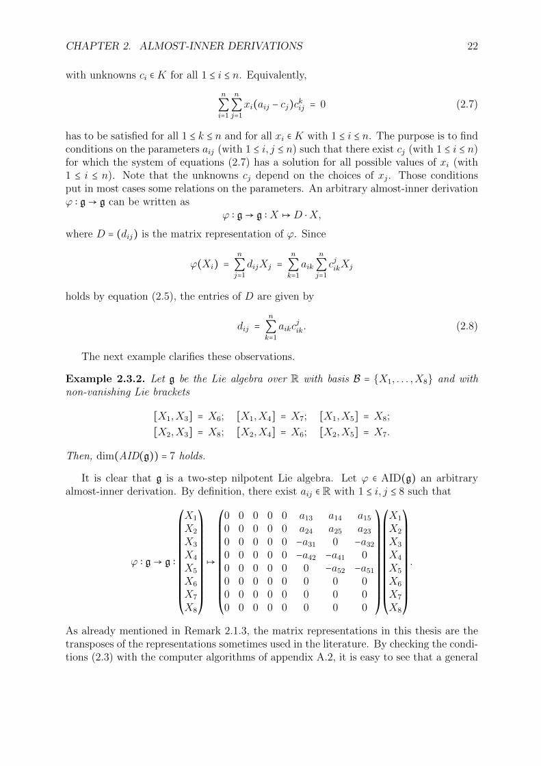
Example 2.3.2. Let g be the Lie algebra over R with basis B = {X1, . . . ,X8} and withnon-vanishing Lie brackets
[X1,X3] = X6; [X1,X4] = X7; [X1,X5] = X8;
[X2,X3] = X8; [X2,X4] = X6; [X2,X5] = X7.
Then, dim(AID(g)) = 7 holds.
It is clear that g is a two-step nilpotent Lie algebra. Let ϕ ∈ AID(g) an arbitraryalmost-inner derivation. By definition, there exist aij ∈ R with 1 ≤ i, j ≤ 8 such that
ϕ ∶ g→ g ∶
⎛⎜⎜⎜⎜⎜⎜⎜⎜⎜⎜⎜⎜⎜⎝
X1
X2
X3
X4
X5
X6
X7
X8
⎞⎟⎟⎟⎟⎟⎟⎟⎟⎟⎟⎟⎟⎟⎠
↦
⎛⎜⎜⎜⎜⎜⎜⎜⎜⎜⎜⎜⎜⎜⎝
0 0 0 0 0 a13 a14 a150 0 0 0 0 a24 a25 a230 0 0 0 0 −a31 0 −a320 0 0 0 0 −a42 −a41 00 0 0 0 0 0 −a52 −a510 0 0 0 0 0 0 00 0 0 0 0 0 0 00 0 0 0 0 0 0 0
⎞⎟⎟⎟⎟⎟⎟⎟⎟⎟⎟⎟⎟⎟⎠
⎛⎜⎜⎜⎜⎜⎜⎜⎜⎜⎜⎜⎜⎜⎝
X1
X2
X3
X4
X5
X6
X7
X8
⎞⎟⎟⎟⎟⎟⎟⎟⎟⎟⎟⎟⎟⎟⎠
.
As already mentioned in Remark 2.1.3, the matrix representations in this thesis are thetransposes of the representations sometimes used in the literature. By checking the condi-tions (2.3) with the computer algorithms of appendix A.2, it is easy to see that a general
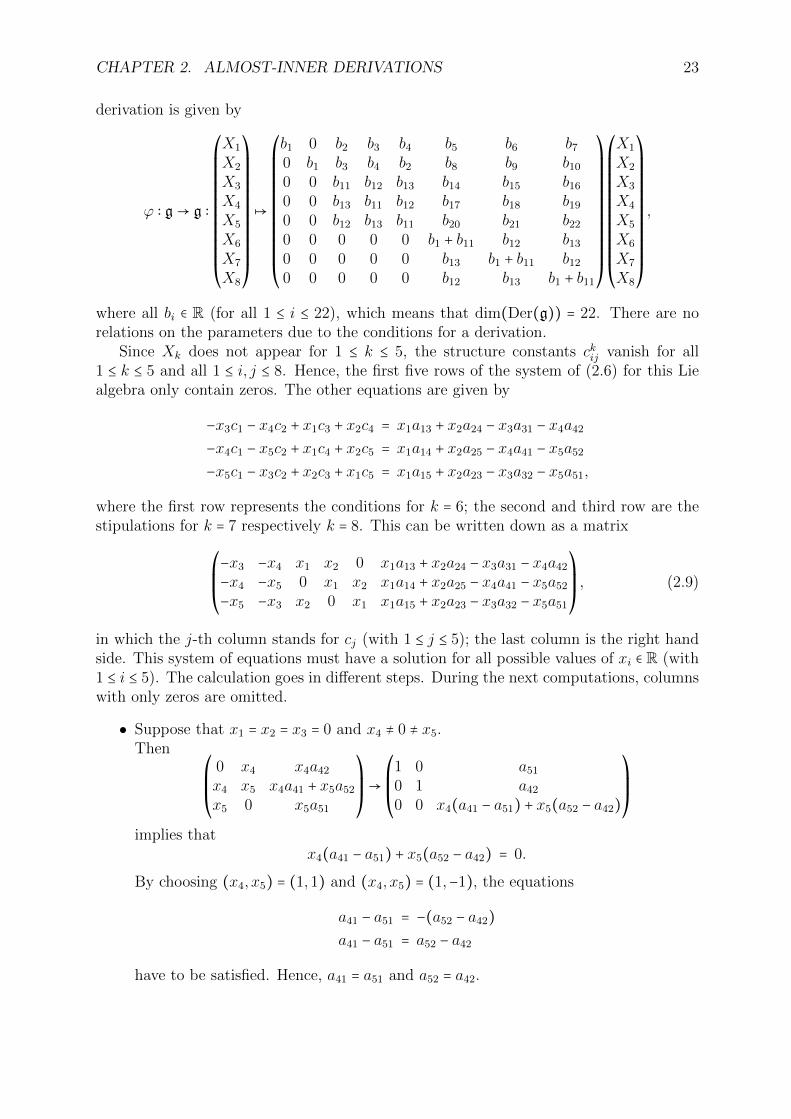
CHAPTER 2. ALMOST-INNER DERIVATIONS 23
derivation is given by
ϕ ∶ g→ g ∶
⎛⎜⎜⎜⎜⎜⎜⎜⎜⎜⎜⎜⎜⎜⎝
X1
X2
X3
X4
X5
X6
X7
X8
⎞⎟⎟⎟⎟⎟⎟⎟⎟⎟⎟⎟⎟⎟⎠
↦
⎛⎜⎜⎜⎜⎜⎜⎜⎜⎜⎜⎜⎜⎜⎝
b1 0 b2 b3 b4 b5 b6 b70 b1 b3 b4 b2 b8 b9 b100 0 b11 b12 b13 b14 b15 b160 0 b13 b11 b12 b17 b18 b190 0 b12 b13 b11 b20 b21 b220 0 0 0 0 b1 + b11 b12 b130 0 0 0 0 b13 b1 + b11 b120 0 0 0 0 b12 b13 b1 + b11
⎞⎟⎟⎟⎟⎟⎟⎟⎟⎟⎟⎟⎟⎟⎠
⎛⎜⎜⎜⎜⎜⎜⎜⎜⎜⎜⎜⎜⎜⎝
X1
X2
X3
X4
X5
X6
X7
X8
⎞⎟⎟⎟⎟⎟⎟⎟⎟⎟⎟⎟⎟⎟⎠
,
where all bi ∈ R (for all 1 ≤ i ≤ 22), which means that dim(Der(g)) = 22. There are norelations on the parameters due to the conditions for a derivation.
Since Xk does not appear for 1 ≤ k ≤ 5, the structure constants ckij vanish for all1 ≤ k ≤ 5 and all 1 ≤ i, j ≤ 8. Hence, the first five rows of the system of (2.6) for this Liealgebra only contain zeros. The other equations are given by
−x3c1 − x4c2 + x1c3 + x2c4 = x1a13 + x2a24 − x3a31 − x4a42−x4c1 − x5c2 + x1c4 + x2c5 = x1a14 + x2a25 − x4a41 − x5a52−x5c1 − x3c2 + x2c3 + x1c5 = x1a15 + x2a23 − x3a32 − x5a51,
where the first row represents the conditions for k = 6; the second and third row are thestipulations for k = 7 respectively k = 8. This can be written down as a matrix
⎛⎜⎜⎝
−x3 −x4 x1 x2 0 x1a13 + x2a24 − x3a31 − x4a42−x4 −x5 0 x1 x2 x1a14 + x2a25 − x4a41 − x5a52−x5 −x3 x2 0 x1 x1a15 + x2a23 − x3a32 − x5a51
⎞⎟⎟⎠, (2.9)
in which the j-th column stands for cj (with 1 ≤ j ≤ 5); the last column is the right handside. This system of equations must have a solution for all possible values of xi ∈ R (with1 ≤ i ≤ 5). The calculation goes in different steps. During the next computations, columnswith only zeros are omitted.
• Suppose that x1 = x2 = x3 = 0 and x4 ≠ 0 ≠ x5.Then
⎛⎜⎜⎝
0 x4 x4a42x4 x5 x4a41 + x5a52x5 0 x5a51
⎞⎟⎟⎠→
⎛⎜⎜⎝
1 0 a510 1 a420 0 x4(a41 − a51) + x5(a52 − a42)
⎞⎟⎟⎠
implies thatx4(a41 − a51) + x5(a52 − a42) = 0.
By choosing (x4, x5) = (1,1) and (x4, x5) = (1,−1), the equations
a41 − a51 = −(a52 − a42)a41 − a51 = a52 − a42
have to be satisfied. Hence, a41 = a51 and a52 = a42.
CHAPTER 2. ALMOST-INNER DERIVATIONS 24
• Consider x1 = x2 = x4 = 0 and x3 ≠ 0 ≠ x5.Analogously, it follows from
⎛⎜⎜⎝
x3 0 x3a310 x5 x5a52x5 x3 x3a32 + x5a51
⎞⎟⎟⎠→
⎛⎜⎜⎝
1 0 a310 1 a520 0 x3(a32 − a52) + x5(a51 − a31)
⎞⎟⎟⎠
that a32 = a52 and a51 = a31.
• Let x3 = x4 = x5 = 0 and x1 ≠ 0 ≠ x2. The system then becomes
⎛⎜⎜⎝
x1 x2 0 x1a13 + x2a240 x1 x2 x1a14 + x2a25x2 0 x1 x1a15 + x2a23
⎞⎟⎟⎠
→⎛⎜⎜⎝
x1 x2 0 x1a13 + x2a240 x1 x2 x1a14 + x2a250 −x22 x21 x21a15 + x1x2(a23 − a13) − x22a24
⎞⎟⎟⎠
→⎛⎜⎜⎝
x21 0 −x22 x21a13 + x1x2(a24 − a14) − x22a250 x1 x2 x1a14 + x2a250 0 x31 + x32 x31a15 + x21x2(a23 − a13) + x1x22(a14 − a24) + x32a25
⎞⎟⎟⎠.
This system of equations has a solution if and only if
x31a15 + x21x2(a23 − a13) + x1x22(a14 − a24) + x32a25 = 0
holds whenever x31 = −x32 and x1 ≠ 0 ≠ x2. Working over R, this gives one extracondition
a15 − a23 + a13 + a14 − a24 − a25 = 0.
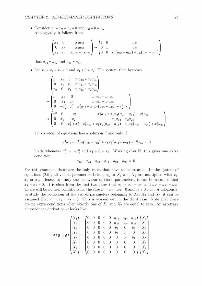
For this example, those are the only cases that have to be treated. In the system ofequations (2.9), all visible parameters belonging to X1 and X2 are multiplied with x3,x4 or x5. Hence, to study the behaviour of those parameters, it can be assumed thatx1 = x2 = 0. It is clear from the first two cases that a31 = a41 = a51 and a32 = a42 = a52.There will be no new conditions for the case x1 = x2 = x5 = 0 and x3 ≠ 0 ≠ x4. Analogously,to study the behaviour of the visible parameters belonging to X3, X4 and X5, it can beassumed that x3 = x4 = x5 = 0. This is worked out in the third case. Note that thereare no extra conditions when exactly one of X1 and X2 are equal to zero. An arbitraryalmost-inner derivation ϕ looks like
ϕ ∶ g→ g ∶
⎛⎜⎜⎜⎜⎜⎜⎜⎜⎜⎜⎜⎜⎜⎝
X1
X2
X3
X4
X5
X6
X7
X8
⎞⎟⎟⎟⎟⎟⎟⎟⎟⎟⎟⎟⎟⎟⎠
↦
⎛⎜⎜⎜⎜⎜⎜⎜⎜⎜⎜⎜⎜⎜⎝
0 0 0 0 0 a13 a14 a150 0 0 0 0 a24 a25 a230 0 0 0 0 b1 0 b20 0 0 0 0 b2 b1 00 0 0 0 0 0 b2 b10 0 0 0 0 0 0 00 0 0 0 0 0 0 00 0 0 0 0 0 0 0
⎞⎟⎟⎟⎟⎟⎟⎟⎟⎟⎟⎟⎟⎟⎠
⎛⎜⎜⎜⎜⎜⎜⎜⎜⎜⎜⎜⎜⎜⎝
X1
X2
X3
X4
X5
X6
X7
X8
⎞⎟⎟⎟⎟⎟⎟⎟⎟⎟⎟⎟⎟⎟⎠
,
CHAPTER 2. ALMOST-INNER DERIVATIONS 25
where a13, a14, a15, a24, a25, b1 and b2 all belong to the field R and where
a23 = a13 + a14 − a24 + a15 − a25.
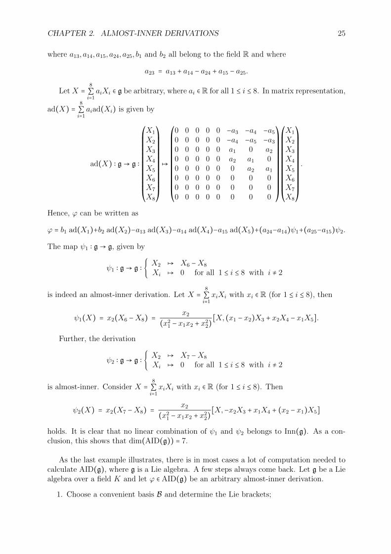
Let X =8
∑i=1aiXi ∈ g be arbitrary, where ai ∈ R for all 1 ≤ i ≤ 8. In matrix representation,
ad(X) =8
∑i=1aiad(Xi) is given by
ad(X) ∶ g→ g ∶
⎛⎜⎜⎜⎜⎜⎜⎜⎜⎜⎜⎜⎜⎜⎝
X1
X2
X3
X4
X5
X6
X7
X8
⎞⎟⎟⎟⎟⎟⎟⎟⎟⎟⎟⎟⎟⎟⎠
↦
⎛⎜⎜⎜⎜⎜⎜⎜⎜⎜⎜⎜⎜⎜⎝
0 0 0 0 0 −a3 −a4 −a50 0 0 0 0 −a4 −a5 −a30 0 0 0 0 a1 0 a20 0 0 0 0 a2 a1 00 0 0 0 0 0 a2 a10 0 0 0 0 0 0 00 0 0 0 0 0 0 00 0 0 0 0 0 0 0
⎞⎟⎟⎟⎟⎟⎟⎟⎟⎟⎟⎟⎟⎟⎠
⎛⎜⎜⎜⎜⎜⎜⎜⎜⎜⎜⎜⎜⎜⎝
X1
X2
X3
X4
X5
X6
X7
X8
⎞⎟⎟⎟⎟⎟⎟⎟⎟⎟⎟⎟⎟⎟⎠
.
Hence, ϕ can be written as
ϕ = b1 ad(X1)+b2 ad(X2)−a13 ad(X3)−a14 ad(X4)−a15 ad(X5)+(a24−a14)ψ1+(a25−a15)ψ2.
The map ψ1 ∶ g→ g, given by
ψ1 ∶ g→ g ∶ { X2 ↦ X6 −X8
Xi ↦ 0 for all 1 ≤ i ≤ 8 with i ≠ 2
is indeed an almost-inner derivation. Let X =8
∑i=1xiXi with xi ∈ R (for 1 ≤ i ≤ 8), then
ψ1(X) = x2(X6 −X8) = x2(x21 − x1x2 + x22)
[X, (x1 − x2)X3 + x2X4 − x1X5].
Further, the derivation
ψ2 ∶ g→ g ∶ { X2 ↦ X7 −X8
Xi ↦ 0 for all 1 ≤ i ≤ 8 with i ≠ 2
is almost-inner. Consider X =8
∑i=1xiXi with xi ∈ R (for 1 ≤ i ≤ 8). Then
ψ2(X) = x2(X7 −X8) = x2(x21 − x1x2 + x22)
[X,−x2X3 + x1X4 + (x2 − x1)X5]
holds. It is clear that no linear combination of ψ1 and ψ2 belongs to Inn(g). As a con-clusion, this shows that dim(AID(g)) = 7.
As the last example illustrates, there is in most cases a lot of computation needed tocalculate AID(g), where g is a Lie algebra. A few steps always come back. Let g be a Liealgebra over a field K and let ϕ ∈ AID(g) be an arbitrary almost-inner derivation.
1. Choose a convenient basis B and determine the Lie brackets;
CHAPTER 2. ALMOST-INNER DERIVATIONS 26
2. Set up the matrix representation of ϕ with parameters with respect to B;
3. Derive relations on the parameters by conditions for
• a derivation
• an almost-inner derivation;
4. Determine the linearly independent almost-inner derivations and check.
The first step was very easy in the example, because this was given in advance. How-ever, for some classes of Lie algebras, it is very hard to construct the non-vanishing Liebrackets (this is for example the case in Section 3.4). The second step already gives an up-per bound for the dimension. In the third step, the relations between the parameters arechecked, by combining different conditions. When all relations are revealed, it is possibleto express the dimension of the space of almost-inner derivations. If AID(g) ≠ Inn(g), itis interesting to specify how an almost-inner derivation (which is not inner) looks like. Insome cases, it is possible to obtain a result without going through all the steps. However,this procedure will be very useful to compute AID(g) for the Lie algebras of the classesof Chapter 3.
In many cases, the third step is the hardest one. The conditions due to the definition ofa derivation can be computed using the algorithms of A.2. For an almost-inner derivation,also the system of equations (2.7) has to be satisfied. This system has to hold for allpossible values of the given field. Especially for fields with infinitely many elements,this is difficult to verify. Therefore, it is important to have some properties concerningalmost-inner derivations. This will be elaborated in the next subsection.
2.3.2 Properties to compute the almost-inner derivations
In this subsection, some first results are obtained, which ease the computation of thespace of almost-inner derivations for a given Lie algebra.
Let g be an n-dimensional Lie algebra over a field K with basis B = {X1, . . . ,Xn}and structure constants ckij (where 1 ≤ i, j, k ≤ n). Let ϕ ∈ AID(g) be an almost-innerderivation of g. Then ϕ(Xi) ∈ [Xi,g] holds by definition for all 1 ≤ i ≤ n. Since ϕ is alinear map, it is clear that
dim(AID(g)) ≤n
∑i=1
dim([Xi,g])
holds. This gives an upper bound for dim(AID(g)). Motivated by this equation, thedimension of a basis vector is introduced.
Definition 2.3.3 (Dimension of a basis vector). Let g be a Lie algebra with basis B ={X1, . . . ,Xn}. The dimension of the basis vector Xi is defined as
di ∶= dim([Xi,g]).
Every inner derivation is also almost-inner, hence
dim(Inn(g)) ≤ dim(AID(g)) ≤n
∑i=1
di. (2.10)

CHAPTER 2. ALMOST-INNER DERIVATIONS 27
As explained in the last section, the conditions due to the definition of an almost-innerderivation can force some visible parameters to be equal. When all visible parametersbelonging to the same basis vector has to be the same, the vector is called fixed.
Definition 2.3.4 (Fixed basis vector). Let g be a Lie algebra over a field K with basisB = {X1, . . . ,Xn}. Let ϕ ∈ AID(g) be an almost-inner derivation with parameters aij withrespect to B for 1 ≤ i, j ≤ n. A basis vector Xj is fixed if there exists a value aj ∈ K sothat aj = aij for all visible parameters belonging to Xj. Then aj is called the ‘fixed value’for Xj.
The hard part in this theoretical description is to find which basis vectors are fixed.However, in some cases, the conditions are trivially satisfied, as is stated in the followingimportant remark. It will be useful in Chapter 3.
Remark 2.3.5. Let g be a Lie algebra over a field K with basis B = {X1, . . . ,Xn}. Letϕ ∈ AID(g) be an almost-inner derivation with parameters aij with respect to B for all1 ≤ i, j ≤ n. Suppose that Xj is a basis vector with at most one visible parameter. ThenXj is fixed by definition.
This is for example the case for all basis vectors in the centre. Whether or not abasis vector is fixed, depends on the choice of a basis. However, when all basis vectors arefixed, there is a nice relation with a general property of the Lie algebra, namely that everyalmost-inner derivation is an inner derivation. This fact is stated in the next lemma.
Lemma 2.3.6. Let g be a n-dimensional Lie algebra over a field K with basis B ={X1, . . . ,Xn}. Then the equation
Inn(g) = CAID(g) = AID(g)
holds if and only if every basis vector Xi is fixed (1 ≤ i ≤ n).
Proof. Let ϕ ∈ AID(g) be an arbitrary almost-inner derivation with matrix representationD = (dij). Suppose first that Inn(g) = AID(g). Then ϕ is an inner derivation. Hence, there
exist values ak ∈K (with 1 ≤ k ≤ n) such that ϕ =n
∑i=kakad(Xk). In matrix representation,
this implies that
dij =n
∑k=1
−akcjik
holds. It follows from equation (2.8) that every basis vector Xk is fixed with fixed value−ak (where 1 ≤ k ≤ n).
Conversely, if every basis vector Xk is fixed with fixed value ak ∈K (for 1 ≤ k ≤ n), thematrix representation of ϕ is given by
dij =n
∑k=1
akcjik.
Hence, ϕ is a linear combination of the inner derivations ad(Xk) with coefficients −ak (for1 ≤ k ≤ n). Since ϕ ∈ AID(g) was arbitrary, this completes the proof.
CHAPTER 2. ALMOST-INNER DERIVATIONS 28
Let g be an n-dimensional Lie algebra over a field K with basis B = {X1, . . . ,Xn}.To prove that a basis vector Xi is fixed, it suffices to show that aji = ali for all visibleparameters belonging to Xi. Next two lemmas are very technical and not very practicalat first sight. They give sufficient conditions for some visible parameters belonging to thesame basis vector to be equal, based on the equations (2.7). By applying those lemmasseveral times, it is possible to prove that some basis vectors are fixed. This approach willbe used frequently in the next chapter.
Lemma 2.3.7. Let g be a Lie algebra over K with basis B = {X1, . . . ,Xn} and structureconstants ckij. Let ϕ ∈ AID(g) be an almost-inner derivation with parameters aij (with1 ≤ i, j, k ≤ n). Let (i, j, k, l) ∈ {1, . . . , n}4 such that the following conditions are satisfied:
• ckij ≠ 0 and ckil ≠ 0;
• ckpj = ckpl = 0 for all 1 ≤ p ≤ n and p ≠ i.
Then, aji = ali follows.
Proof. There is nothing to show when j = l, so suppose that j ≠ l. By equation (2.7), thecondition
n
∑q=1
n
∑p=1
xq(aqp − cp)crqp = 0
has to be satisfied for all 1 ≤ r ≤ n and for all xq ∈K with 1 ≤ q ≤ n. Let xj ≠ 0 and xl ≠ 0and choose xq = 0 when q ≠ j, l. The equation for the basis vector Xk becomes
n
∑p=1
xj(ajp − cp)ckjp +n
∑p=1
xl(alp − cp)cklp = 0.
The values cp (with 1 ≤ p ≤ n) depend on the chosen values of xq (with 1 ≤ q ≤ n). Byassumption on the structure constants, this means that
xj(aji − ci)ckji + xl(ali − ci)ckli = 0
holds for all xj ≠ 0 ≠ xl, which is equivalent to
xjajickji + xlalickli = (xjckji + xlckli)ci.
Choose now xj = −xl ckli
ckji, then it follows that
xlckli(−aji + ali) = 0.
Since xl ≠ 0 and ckji ≠ 0, this implies that aji = ali.
Many Lie algebras satisfy the conditions of the lemma. In particular, this is true whenthe basis vector Xk appears exactly twice, namely for the pairs {Xi,Xj} and {Xi,Xl}.In this case, it follows that aji = ali. The same result is obtained when the conditions areslightly changed.
Lemma 2.3.8. Let g be a Lie algebra over K with basis B = {X1, . . . ,Xn} and structureconstants ckij. Let ϕ ∈ AID(g) be an almost-inner derivation with parameters aij (where1 ≤ i, j, k ≤ n). Let (i, j, k, l,m) ∈ {1, . . . , n}5 with k ≠m such that the following conditionsare satisfied:
CHAPTER 2. ALMOST-INNER DERIVATIONS 29
• ckij ≠ 0 and cmil ≠ 0;
• ckpj = cmpl = 0 for all 1 ≤ p ≤ n with p ≠ i;
• ckpl = cmpj = 0 for all 1 ≤ p ≤ n.
Then, aji = ali follows.
Proof. For j = l, the result immediately follows, so suppose that j ≠ l. Again, the condition
n
∑q=1
n
∑p=1
xq(aqp − cp)crqp = 0
has to be satisfied for all 1 ≤ r ≤ n and for all xq ∈K with 1 ≤ q ≤ n. Fix xj ≠ 0 and xl ≠ 0and set xq = 0 for all q ≠ j, l. In particular, the equations for the basis vectors Xk and Xm
become
n
∑p=1
xj(ajp − cp)ckjp +n
∑p=1
xl(alp − cp)cklp = 0
n
∑p=1
xj(ajp − cp)cmjp +n
∑p=1
xl(alp − cp)cmlp = 0.
Note that the values cp (with 1 ≤ p ≤ n) depend on the chosen values of xq (with 1 ≤ q ≤ n).By assumption on the structure constants, this further reduces to
xj(aji − ci)ckji = 0
xl(ali − ci)cmli = 0,
from which the result easily follows, since ckij ≠ 0 ≠ cmil and xj ≠ 0 ≠ xl.
Although the conditions of this lemma seem to be demanding, next chapter shows thatthey are satisfied for a lot of Lie algebras. In particular, suppose that the basis vector Xk
appears once. Then all conditions on the structure constants ckij are satisfied (where 1 ≤i, j ≤ n). When Xk and Xm both appear once, namely for the pairs {Xi,Xj} respectively{Xi,Xl}, it follows from the lemma that aji = ali. This situation will frequently occur forthe Lie algebras studied in Chapter 3. Next lemma states that an almost-inner derivationof a Lie algebra induces an almost-inner derivation of the quotient of that Lie algebra byan ideal.
Lemma 2.3.9. Let g be a Lie algebra with ideal h. Let ϕ ∈ AID(g) be an almost-innerderivation of g. Then ϕ(h) ⊆ h. Moreover, ϕ induces an almost-inner derivation of g/h.
Proof. Choose X ∈ h arbitrarily. By definition of an almost-inner derivation, it followsthat
ϕ(X) ∈ [X,g] ⊆ [h,g] ⊆ h.
Since X ∈ h was arbitrary, this proves that ϕ(h) ⊆ h. Define
ϕ ∶ g/h→ g/h ∶X + h↦ ϕ(X + h) ∶= ϕ(X) + h.
CHAPTER 2. ALMOST-INNER DERIVATIONS 30
This is a well-defined linear map due to the first statement. Choose X + h, Y + h ∈ g/harbitrarily. Then
ϕ([X + h, Y + h]) = ϕ([X,Y ] + h) = ϕ([X,Y ]) + h
holds, as well as
[ϕ(X + h), Y + h] + [X + h, ϕ(Y + h)] = [ϕ(X) + h, Y + h] + [X + h, ϕ(Y ) + h]= [ϕ(X), Y ] + h + [X,ϕ(Y )] + h.
Combining these equations and using that ϕ is a derivation of g, it follows that ϕ is aderivation of g/h. Let X + h ∈ g/h be arbitrary. Since ϕ is an almost-inner derivation ofg, there exists Y ∈ g such that ϕ(X) = [X,Y ]. Hence,
ϕ(X + h) = ϕ(X) + h = [X,Y ] + h = [X + h, Y + h],
which shows that ϕ is an almost-inner derivation of g/h.
When a Lie algebra is the direct sum of two Lie algebras, the set of almost-innerderivations AID(g) satisfy an easy rule. This is worked out in the following proposition.
Proposition 2.3.10. Let g = g1⊕ g2 be the direct sum of two Lie algebras g1 and g2 overthe same field. Then
AID(g) = AID(g1)⊕AID(g2)holds.
Proof. The proof goes in two steps. First, let ϕ ∈ AID(g) be an almost-inner derivationand let X ∈ g be arbitrary. Then X = X1 + X2, where X1 ∈ g1 and X2 ∈ g2. Sinceϕ ∈ AID(g), there exists Y = Y1+Y2 ∈ g (with Y1 ∈ g1 and Y2 ∈ g2) such that ϕ(X) = [X,Y ].By construction,
ϕ(X) = [X,Y ]= [X1 +X2, Y1 + Y2]= [X1, Y1] + [X1, Y2] + [X2, Y1] + [X2, Y2]= [X1, Y1] + [X2, Y2],
where the last equality holds since [g1,g2] = 0, by definition of the direct sum. This meansthat ϕ1 ∶= ϕ∣g1 is an almost-inner derivation of g1. Analogously, ϕ2 ∶= ϕ∣g2 ∈ AID(g2) issatisfied. Hence, ϕ can be written as ϕ = ϕ1 ⊕ ϕ2, which is defined as
ϕ ∶ g1 ⊕ g2 → g1 ⊕ g2 ∶X1 +X2 ↦ (ϕ1 ⊕ ϕ2)(X1 +X2) = ϕ1(X1) + ϕ2(X2).
Moreover, let X =X1+X2 ∈ g be arbitrary, with X1 ∈ g1 and X2 ∈ g2. Let ϕ1 ∈ AID(g1)⊕0and ϕ2 ∈ 0⊕AID(g1) be arbitrary. Then
[ϕ1, ϕ2](X) = [ϕ1, ϕ2](X1 +X2)= [ϕ1, ϕ2](X1) + [ϕ1, ϕ2](X2)= ϕ1ϕ2(X1) − ϕ2ϕ1(X1) + ϕ1ϕ2(X2) − ϕ2ϕ1(X2)= 0
CHAPTER 2. ALMOST-INNER DERIVATIONS 31
follows. This means that [AID(g1),AID(g2)] = 0 holds and completes the proof of thefirst inclusion.
Conversely, let ϕ1 +ϕ2 ∈ AID(g1)⊕AID(g1) be arbitrary, where ϕ1 ∈ AID(g1)⊕ 0 andϕ2 ∈ 0⊕AID(g2). Define the map (ϕ1 + ϕ2) as
(ϕ1 + ϕ2) ∶ g→ g ∶X =X1 +X2 ↦ ϕ1(X1) + ϕ2(X2),
where X1 ∈ g1 and X2 ∈ g2. By definition of an almost-inner derivation of g, there existY1 ∈ g1 and Y2 ∈ g2 such that ϕ1(X1) = [X1, Y1] and ϕ2(X2) = [X2, Y2]. Note that thesebrackets are in g. Since [X1, Y2] = 0 = [X2, Y1], it follows that
(ϕ1 + ϕ2)(X) ∶= ϕ1(X1) + ϕ2(X2)= [X1, Y1] + [X2, Y2]= [X1, Y1] + [X2, Y2] + [X1, Y2] + [X2, Y1]= [X1 +X2, Y1 + Y2].
Hence, the map ϕ1 + ϕ2 defines an almost-inner derivation of g.
In particular, this proposition is useful for Lie algebras g = g1⊕g2, where g2 is abelian.In this case, AID(g) = AID(g1) holds. An example of this situation is postponed to thenext chapter.
Chapter 3
Different classes of Lie algebras
The procedure to compute the almost-inner derivations of a Lie algebra will be used fordifferent classes of Lie algebras. In particular, it is studied for which of these classes ofLie algebras there exist non-inner almost-inner derivations. The first section concerns(complex) Lie algebras of dimension n ≤ 4. For these Lie algebras, all almost-innerderivations are inner. In Section 3.2, filiform Lie algebras are studied. For such a Liealgebra g which is also metabelian, the dimension of AID(g) is at most one more than thedimension of Inn(g). Further, two-step nilpotent Lie algebras can be defined by a graph;this is worked out in the following section. The fourth section is about free nilpotent Liealgebras; results for this class are only obtained when the nilindex is two or three. Finally,(strictly) uppertriangular matrices are treated. For the Lie algebras studied in the lastthree classes, the only almost-inner derivations are the inner ones. Except for the firstand last class, all types are examples of nilpotent Lie algebras. This is since the geometricmotivation only holds for those Lie algebras.
3.1 Low-dimensional Lie algebras
In this section, all non-isomorphic complex Lie algebras of dimension n ≤ 4 are listed. Itis clear that a one-dimensional Lie algebra can not have non-zero brackets. When thedimension is equal to n = 2, next proposition even holds for an arbitrary field. This is awell-known result, see for example [8, page 20].
Proposition 3.1.1. Let K be an arbitrary field and let g be a non-abelian two-dimensionalLie algebra over K. Then there exists a basis B = {X1,X2} such that the Lie bracket isgiven by [X1,X2] = X1. Hence, for every field K, there is, up to isomorphism, a uniquenon-abelian two-dimensional Lie algebra over K.
Proof. Let g be a non-abelian two-dimensional Lie algebra over the field K. Let B ={X,Y } be a basis of g. Since g is non-abelian, [g,g] = span{[X,Y ]} is one-dimensional.Let X1 ∈ [g,g] be non-zero and extend to a basis {X1, Y } of the vector space g. Then,[X1, Y ] ∈ [g,g] is non-zero, since [X1, Y ] spans [g,g]. This means that [X1, Y ] = kX1 fork ∈K∗. For X2 ∶= k−1Y , the Lie bracket of g is given by [X1,X2] =X1, where {X1,X2} isa basis of g. It is easy to check that this indeed defines a Lie algebra.
The unique non-abelian two dimensional Lie algebra over K is denoted by r2(K) oraff(K). For Lie algebras of dimension n ≥ 3, it is difficult to classify the Lie algebras over
32
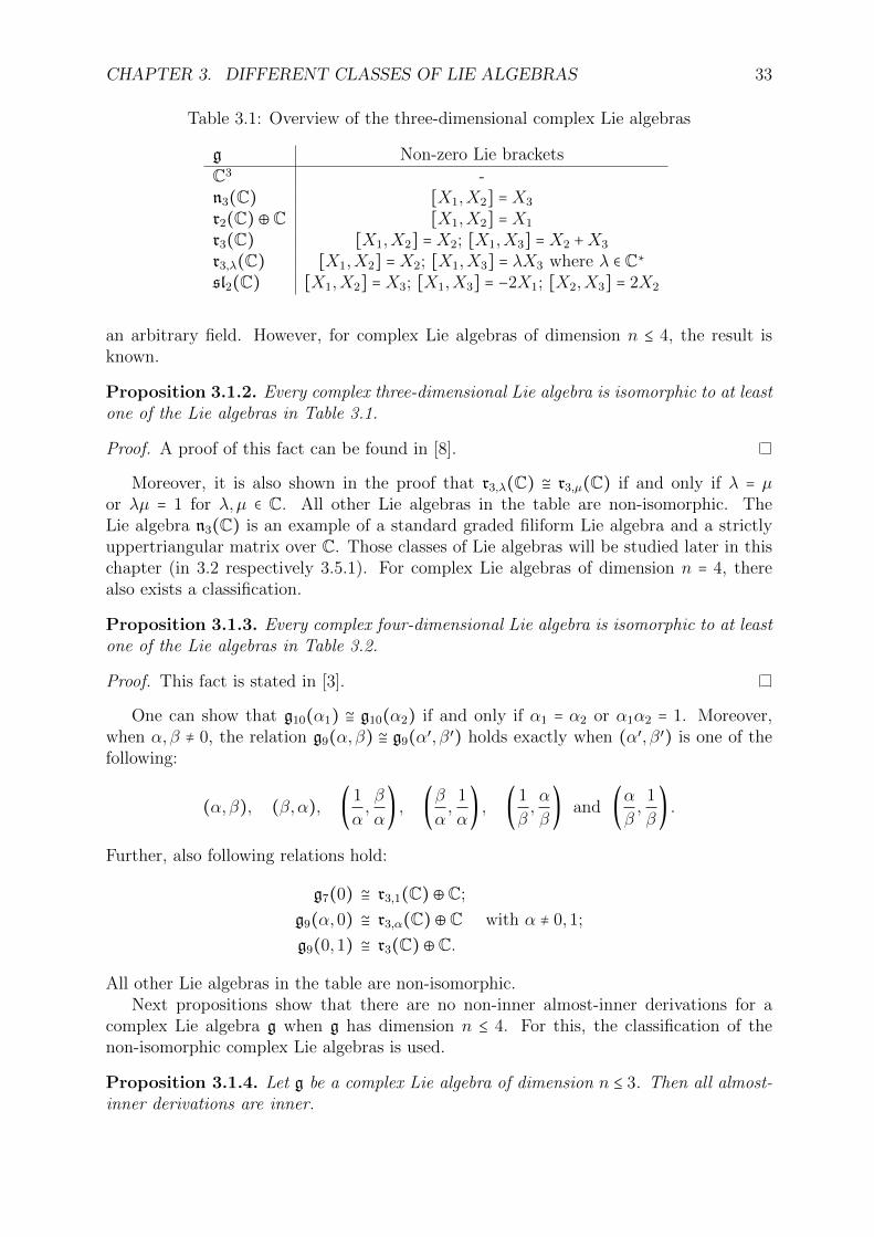
CHAPTER 3. DIFFERENT CLASSES OF LIE ALGEBRAS 33
Table 3.1: Overview of the three-dimensional complex Lie algebras
g Non-zero Lie bracketsC3 -n3(C) [X1,X2] =X3
r2(C)⊕C [X1,X2] =X1
r3(C) [X1,X2] =X2; [X1,X3] =X2 +X3
r3,λ(C) [X1,X2] =X2; [X1,X3] = λX3 where λ ∈ C∗
sl2(C) [X1,X2] =X3; [X1,X3] = −2X1; [X2,X3] = 2X2
an arbitrary field. However, for complex Lie algebras of dimension n ≤ 4, the result isknown.
Proposition 3.1.2. Every complex three-dimensional Lie algebra is isomorphic to at leastone of the Lie algebras in Table 3.1.
Proof. A proof of this fact can be found in [8].
Moreover, it is also shown in the proof that r3,λ(C) ≅ r3,µ(C) if and only if λ = µor λµ = 1 for λ,µ ∈ C. All other Lie algebras in the table are non-isomorphic. TheLie algebra n3(C) is an example of a standard graded filiform Lie algebra and a strictlyuppertriangular matrix over C. Those classes of Lie algebras will be studied later in thischapter (in 3.2 respectively 3.5.1). For complex Lie algebras of dimension n = 4, therealso exists a classification.
Proposition 3.1.3. Every complex four-dimensional Lie algebra is isomorphic to at leastone of the Lie algebras in Table 3.2.
Proof. This fact is stated in [3].
One can show that g10(α1) ≅ g10(α2) if and only if α1 = α2 or α1α2 = 1. Moreover,when α,β ≠ 0, the relation g9(α,β) ≅ g9(α′, β′) holds exactly when (α′, β′) is one of thefollowing:
(α,β), (β,α), ( 1
α,β
α) , (β
α,
1
α) , ( 1
β,α
β) and (α
β,
1
β) .
Further, also following relations hold:
g7(0) ≅ r3,1(C)⊕C;
g9(α,0) ≅ r3,α(C)⊕C with α ≠ 0,1;
g9(0,1) ≅ r3(C)⊕C.
All other Lie algebras in the table are non-isomorphic.Next propositions show that there are no non-inner almost-inner derivations for a
complex Lie algebra g when g has dimension n ≤ 4. For this, the classification of thenon-isomorphic complex Lie algebras is used.
Proposition 3.1.4. Let g be a complex Lie algebra of dimension n ≤ 3. Then all almost-inner derivations are inner.
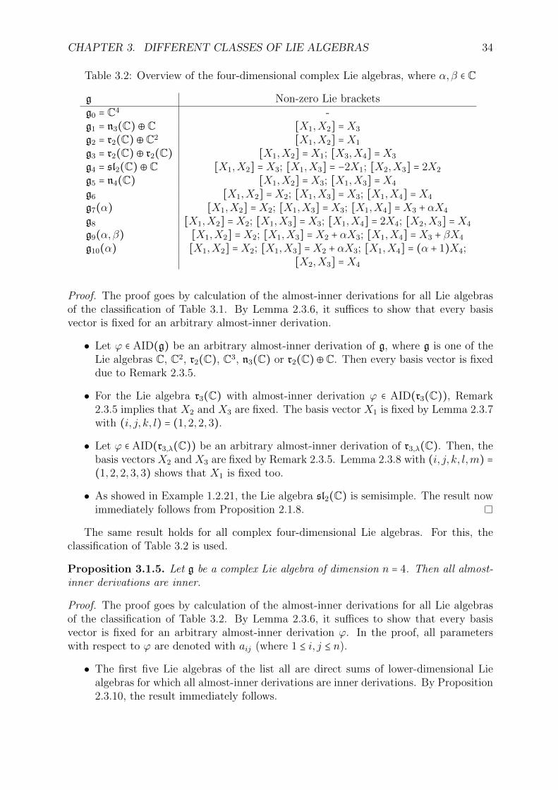
CHAPTER 3. DIFFERENT CLASSES OF LIE ALGEBRAS 34
Table 3.2: Overview of the four-dimensional complex Lie algebras, where α,β ∈ C
g Non-zero Lie bracketsg0 = C4 -g1 = n3(C)⊕C [X1,X2] =X3
g2 = r2(C)⊕C2 [X1,X2] =X1
g3 = r2(C)⊕ r2(C) [X1,X2] =X1; [X3,X4] =X3
g4 = sl2(C)⊕C [X1,X2] =X3; [X1,X3] = −2X1; [X2,X3] = 2X2
g5 = n4(C) [X1,X2] =X3; [X1,X3] =X4
g6 [X1,X2] =X2; [X1,X3] =X3; [X1,X4] =X4
g7(α) [X1,X2] =X2; [X1,X3] =X3; [X1,X4] =X3 + αX4
g8 [X1,X2] =X2; [X1,X3] =X3; [X1,X4] = 2X4; [X2,X3] =X4
g9(α,β) [X1,X2] =X2; [X1,X3] =X2 + αX3; [X1,X4] =X3 + βX4
g10(α) [X1,X2] =X2; [X1,X3] =X2 + αX3; [X1,X4] = (α + 1)X4;[X2,X3] =X4
Proof. The proof goes by calculation of the almost-inner derivations for all Lie algebrasof the classification of Table 3.1. By Lemma 2.3.6, it suffices to show that every basisvector is fixed for an arbitrary almost-inner derivation.
• Let ϕ ∈ AID(g) be an arbitrary almost-inner derivation of g, where g is one of theLie algebras C, C2, r2(C), C3, n3(C) or r2(C)⊕C. Then every basis vector is fixeddue to Remark 2.3.5.
• For the Lie algebra r3(C) with almost-inner derivation ϕ ∈ AID(r3(C)), Remark2.3.5 implies that X2 and X3 are fixed. The basis vector X1 is fixed by Lemma 2.3.7with (i, j, k, l) = (1,2,2,3).
• Let ϕ ∈ AID(r3,λ(C)) be an arbitrary almost-inner derivation of r3,λ(C). Then, thebasis vectors X2 and X3 are fixed by Remark 2.3.5. Lemma 2.3.8 with (i, j, k, l,m) =(1,2,2,3,3) shows that X1 is fixed too.
• As showed in Example 1.2.21, the Lie algebra sl2(C) is semisimple. The result nowimmediately follows from Proposition 2.1.8.
The same result holds for all complex four-dimensional Lie algebras. For this, theclassification of Table 3.2 is used.
Proposition 3.1.5. Let g be a complex Lie algebra of dimension n = 4. Then all almost-inner derivations are inner.
Proof. The proof goes by calculation of the almost-inner derivations for all Lie algebrasof the classification of Table 3.2. By Lemma 2.3.6, it suffices to show that every basisvector is fixed for an arbitrary almost-inner derivation ϕ. In the proof, all parameterswith respect to ϕ are denoted with aij (where 1 ≤ i, j ≤ n).
• The first five Lie algebras of the list all are direct sums of lower-dimensional Liealgebras for which all almost-inner derivations are inner derivations. By Proposition2.3.10, the result immediately follows.
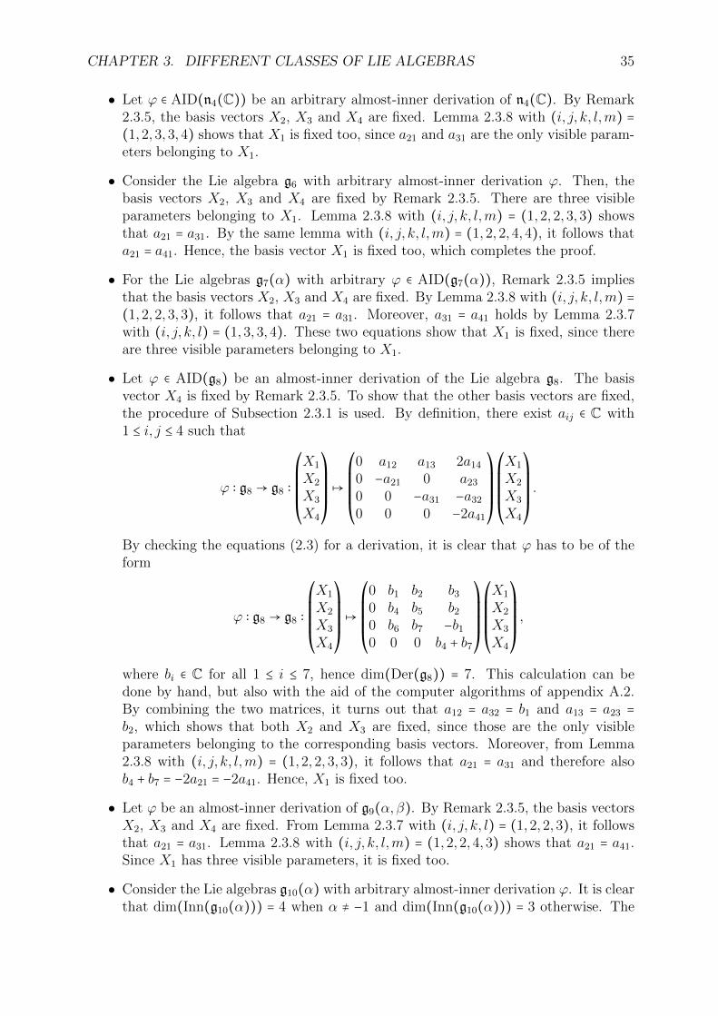
CHAPTER 3. DIFFERENT CLASSES OF LIE ALGEBRAS 35
• Let ϕ ∈ AID(n4(C)) be an arbitrary almost-inner derivation of n4(C). By Remark2.3.5, the basis vectors X2, X3 and X4 are fixed. Lemma 2.3.8 with (i, j, k, l,m) =(1,2,3,3,4) shows that X1 is fixed too, since a21 and a31 are the only visible param-eters belonging to X1.
• Consider the Lie algebra g6 with arbitrary almost-inner derivation ϕ. Then, thebasis vectors X2, X3 and X4 are fixed by Remark 2.3.5. There are three visibleparameters belonging to X1. Lemma 2.3.8 with (i, j, k, l,m) = (1,2,2,3,3) showsthat a21 = a31. By the same lemma with (i, j, k, l,m) = (1,2,2,4,4), it follows thata21 = a41. Hence, the basis vector X1 is fixed too, which completes the proof.
• For the Lie algebras g7(α) with arbitrary ϕ ∈ AID(g7(α)), Remark 2.3.5 impliesthat the basis vectors X2, X3 and X4 are fixed. By Lemma 2.3.8 with (i, j, k, l,m) =(1,2,2,3,3), it follows that a21 = a31. Moreover, a31 = a41 holds by Lemma 2.3.7with (i, j, k, l) = (1,3,3,4). These two equations show that X1 is fixed, since thereare three visible parameters belonging to X1.
• Let ϕ ∈ AID(g8) be an almost-inner derivation of the Lie algebra g8. The basisvector X4 is fixed by Remark 2.3.5. To show that the other basis vectors are fixed,the procedure of Subsection 2.3.1 is used. By definition, there exist aij ∈ C with1 ≤ i, j ≤ 4 such that
ϕ ∶ g8 → g8 ∶⎛⎜⎜⎜⎜⎝
X1
X2
X3
X4
⎞⎟⎟⎟⎟⎠↦
⎛⎜⎜⎜⎜⎝
0 a12 a13 2a140 −a21 0 a230 0 −a31 −a320 0 0 −2a41
⎞⎟⎟⎟⎟⎠
⎛⎜⎜⎜⎜⎝
X1
X2
X3
X4
⎞⎟⎟⎟⎟⎠.
By checking the equations (2.3) for a derivation, it is clear that ϕ has to be of theform
ϕ ∶ g8 → g8 ∶⎛⎜⎜⎜⎜⎝
X1
X2
X3
X4
⎞⎟⎟⎟⎟⎠↦
⎛⎜⎜⎜⎜⎝
0 b1 b2 b30 b4 b5 b20 b6 b7 −b10 0 0 b4 + b7
⎞⎟⎟⎟⎟⎠
⎛⎜⎜⎜⎜⎝
X1
X2
X3
X4
⎞⎟⎟⎟⎟⎠,
where bi ∈ C for all 1 ≤ i ≤ 7, hence dim(Der(g8)) = 7. This calculation can bedone by hand, but also with the aid of the computer algorithms of appendix A.2.By combining the two matrices, it turns out that a12 = a32 = b1 and a13 = a23 =b2, which shows that both X2 and X3 are fixed, since those are the only visibleparameters belonging to the corresponding basis vectors. Moreover, from Lemma2.3.8 with (i, j, k, l,m) = (1,2,2,3,3), it follows that a21 = a31 and therefore alsob4 + b7 = −2a21 = −2a41. Hence, X1 is fixed too.
• Let ϕ be an almost-inner derivation of g9(α,β). By Remark 2.3.5, the basis vectorsX2, X3 and X4 are fixed. From Lemma 2.3.7 with (i, j, k, l) = (1,2,2,3), it followsthat a21 = a31. Lemma 2.3.8 with (i, j, k, l,m) = (1,2,2,4,3) shows that a21 = a41.Since X1 has three visible parameters, it is fixed too.
• Consider the Lie algebras g10(α) with arbitrary almost-inner derivation ϕ. It is clearthat dim(Inn(g10(α))) = 4 when α ≠ −1 and dim(Inn(g10(α))) = 3 otherwise. The
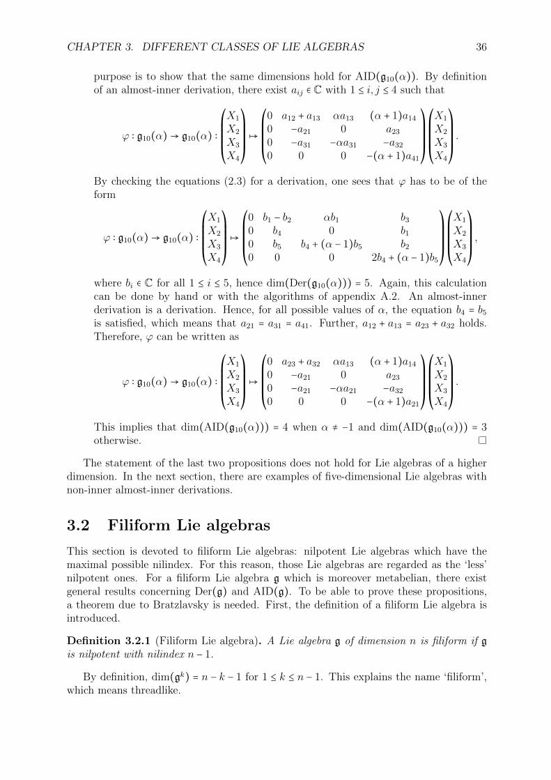
CHAPTER 3. DIFFERENT CLASSES OF LIE ALGEBRAS 36
purpose is to show that the same dimensions hold for AID(g10(α)). By definitionof an almost-inner derivation, there exist aij ∈ C with 1 ≤ i, j ≤ 4 such that
ϕ ∶ g10(α)→ g10(α) ∶⎛⎜⎜⎜⎜⎝
X1
X2
X3
X4
⎞⎟⎟⎟⎟⎠↦
⎛⎜⎜⎜⎜⎝
0 a12 + a13 αa13 (α + 1)a140 −a21 0 a230 −a31 −αa31 −a320 0 0 −(α + 1)a41
⎞⎟⎟⎟⎟⎠
⎛⎜⎜⎜⎜⎝
X1
X2
X3
X4
⎞⎟⎟⎟⎟⎠.
By checking the equations (2.3) for a derivation, one sees that ϕ has to be of theform
ϕ ∶ g10(α)→ g10(α) ∶⎛⎜⎜⎜⎜⎝
X1
X2
X3
X4
⎞⎟⎟⎟⎟⎠↦
⎛⎜⎜⎜⎜⎝
0 b1 − b2 αb1 b30 b4 0 b10 b5 b4 + (α − 1)b5 b20 0 0 2b4 + (α − 1)b5
⎞⎟⎟⎟⎟⎠
⎛⎜⎜⎜⎜⎝
X1
X2
X3
X4
⎞⎟⎟⎟⎟⎠,
where bi ∈ C for all 1 ≤ i ≤ 5, hence dim(Der(g10(α))) = 5. Again, this calculationcan be done by hand or with the algorithms of appendix A.2. An almost-innerderivation is a derivation. Hence, for all possible values of α, the equation b4 = b5is satisfied, which means that a21 = a31 = a41. Further, a12 + a13 = a23 + a32 holds.Therefore, ϕ can be written as
ϕ ∶ g10(α)→ g10(α) ∶⎛⎜⎜⎜⎜⎝
X1
X2
X3
X4
⎞⎟⎟⎟⎟⎠↦
⎛⎜⎜⎜⎜⎝
0 a23 + a32 αa13 (α + 1)a140 −a21 0 a230 −a21 −αa21 −a320 0 0 −(α + 1)a21
⎞⎟⎟⎟⎟⎠
⎛⎜⎜⎜⎜⎝
X1
X2
X3
X4
⎞⎟⎟⎟⎟⎠.
This implies that dim(AID(g10(α))) = 4 when α ≠ −1 and dim(AID(g10(α))) = 3otherwise.
The statement of the last two propositions does not hold for Lie algebras of a higherdimension. In the next section, there are examples of five-dimensional Lie algebras withnon-inner almost-inner derivations.
3.2 Filiform Lie algebras
This section is devoted to filiform Lie algebras: nilpotent Lie algebras which have themaximal possible nilindex. For this reason, those Lie algebras are regarded as the ‘less’nilpotent ones. For a filiform Lie algebra g which is moreover metabelian, there existgeneral results concerning Der(g) and AID(g). To be able to prove these propositions,a theorem due to Bratzlavsky is needed. First, the definition of a filiform Lie algebra isintroduced.
Definition 3.2.1 (Filiform Lie algebra). A Lie algebra g of dimension n is filiform if gis nilpotent with nilindex n − 1.
By definition, dim(gk) = n − k − 1 for 1 ≤ k ≤ n − 1. This explains the name ‘filiform’,which means threadlike.
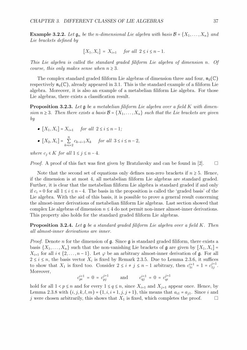
CHAPTER 3. DIFFERENT CLASSES OF LIE ALGEBRAS 37
Example 3.2.2. Let gn be the n-dimensional Lie algebra with basis B = {X1, . . . ,Xn} andLie brackets defined by
[X1,Xi] = Xi+1 for all 2 ≤ i ≤ n − 1.
This Lie algebra is called the standard graded filiform Lie algebra of dimension n. Ofcourse, this only makes sense when n ≥ 3.
The complex standard graded filiform Lie algebras of dimension three and four, n3(C)respectively n4(C), already appeared in 3.1. This is the standard example of a filiform Liealgebra. Moreover, it is also an example of a metabelian filiform Lie algebra. For thoseLie algebras, there exists a classification result.
Proposition 3.2.3. Let g be a metabelian filiform Lie algebra over a field K with dimen-sion n ≥ 3. Then there exists a basis B = {X1, . . . ,Xn} such that the Lie brackets are givenby
• [X1,Xi] =Xi+1 for all 2 ≤ i ≤ n − 1;
• [X2,Xi] =n
∑k=i+2
ck−i−1Xk for all 3 ≤ i ≤ n − 2,
where cj ∈K for all 1 ≤ j ≤ n − 4.
Proof. A proof of this fact was first given by Bratzlavsky and can be found in [2].
Note that the second set of equations only defines non-zero brackets if n ≥ 5. Hence,if the dimension is at most 4, all metabelian filiform Lie algebras are standard graded.Further, it is clear that the metabelian filiform Lie algebra is standard graded if and onlyif ci = 0 for all 1 ≤ i ≤ n− 4. The basis in the proposition is called the ‘graded basis’ of theLie algebra. With the aid of this basis, it is possible to prove a general result concerningthe almost-inner derivations of metabelian filiform Lie algebras. Last section showed thatcomplex Lie algebras of dimension n ≤ 4 do not permit non-inner almost-inner derivations.This property also holds for the standard graded filiform Lie algebras.
Proposition 3.2.4. Let g be a standard graded filiform Lie algebra over a field K. Thenall almost-inner derivations are inner.
Proof. Denote n for the dimension of g. Since g is standard graded filiform, there exists abasis {X1, . . . ,Xn} such that the non-vanishing Lie brackets of g are given by [X1,Xi] =Xi+1 for all i ∈ {2, . . . , n − 1}. Let ϕ be an arbitrary almost-inner derivation of g. For all2 ≤ i ≤ n, the basis vector Xi is fixed by Remark 2.3.5. Due to Lemma 2.3.6, it sufficesto show that X1 is fixed too. Consider 2 ≤ i ≠ j ≤ n − 1 arbitrary, then ci+11i = 1 = cj+11j .Moreover,
ci+1pi = 0 = cj+1pj and ci+1qj = 0 = cj+1qi
hold for all 1 < p ≤ n and for every 1 ≤ q ≤ n, since Xi+1 and Xj+1 appear once. Hence, byLemma 2.3.8 with (i, j, k, l,m) = (1, i, i + 1, j, j + 1), this means that ai1 = aj1. Since i andj were chosen arbitrarily, this shows that X1 is fixed, which completes the proof.
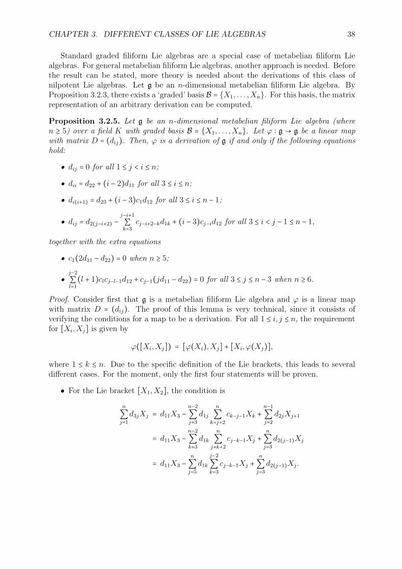
CHAPTER 3. DIFFERENT CLASSES OF LIE ALGEBRAS 38
Standard graded filiform Lie algebras are a special case of metabelian filiform Liealgebras. For general metabelian filiform Lie algebras, another approach is needed. Beforethe result can be stated, more theory is needed about the derivations of this class ofnilpotent Lie algebras. Let g be an n-dimensional metabelian filiform Lie algebra. ByProposition 3.2.3, there exists a ‘graded’ basis B = {X1, . . . ,Xn}. For this basis, the matrixrepresentation of an arbitrary derivation can be computed.
Proposition 3.2.5. Let g be an n-dimensional metabelian filiform Lie algebra (wheren ≥ 5) over a field K with graded basis B = {X1, . . . ,Xn}. Let ϕ ∶ g → g be a linear mapwith matrix D = (dij). Then, ϕ is a derivation of g if and only if the following equationshold:
• dij = 0 for all 1 ≤ j < i ≤ n;
• dii = d22 + (i − 2)d11 for all 3 ≤ i ≤ n;
• di(i+1) = d23 + (i − 3)c1d12 for all 3 ≤ i ≤ n − 1;
• dij = d2(j−i+2) −j−i+1
∑k=3
cj−i+2−kd1k + (i − 3)cj−id12 for all 3 ≤ i < j − 1 ≤ n − 1,
together with the extra equations
• c1(2d11 − d22) = 0 when n ≥ 5;
•j−2
∑l=1
(l + 1)clcj−l−1d12 + cj−1(jd11 − d22) = 0 for all 3 ≤ j ≤ n − 3 when n ≥ 6.
Proof. Consider first that g is a metabelian filiform Lie algebra and ϕ is a linear mapwith matrix D = (dij). The proof of this lemma is very technical, since it consists ofverifying the conditions for a map to be a derivation. For all 1 ≤ i, j ≤ n, the requirementfor [Xi,Xj] is given by
ϕ([Xi,Xj]) = [ϕ(Xi),Xj] + [Xi, ϕ(Xj)],
where 1 ≤ k ≤ n. Due to the specific definition of the Lie brackets, this leads to severaldifferent cases. For the moment, only the first four statements will be proven.
• For the Lie bracket [X1,X2], the condition is
n
∑j=1
d3jXj = d11X3 −n−2
∑j=3
d1jn
∑k=j+2
ck−j−1Xk +n−1
∑j=2
d2jXj+1
= d11X3 −n−2
∑k=3
d1kn
∑j=k+2
cj−k−1Xj +n
∑j=3
d2(j−1)Xj
= d11X3 −n
∑j=5
d1kj−2
∑k=3
cj−k−1Xj +n
∑j=3
d2(j−1)Xj.
CHAPTER 3. DIFFERENT CLASSES OF LIE ALGEBRAS 39
The second and last equality are obtained by renaming respectively replacing thesummands. This means that the following equations have to be satisfied:
d31 = d32 = 0
d33 = d11 + d22d34 = d23
d3j = d2(j−1) −j−2
∑k=3
cj−k−1d1k for all 5 ≤ j ≤ n.
Those are exactly the expressions for d3j that have to be fulfilled in the four firststatements of the proposition, where 1 ≤ j ≤ n.
• The conditions due to [X1,Xi] where 3 ≤ i ≤ n − 2 are given by
n
∑j=1
d(i+1)jXj = d11Xi+1 + d12n
∑j=i+2
cj−i−1Xj +n−1
∑j=2
dijXj+1.
This means that for all 4 ≤ i ≤ n − 1, the equations
n
∑j=1
dijXj = d11Xi + d12n
∑j=i+1
cj−iXj +n
∑j=3
d(i−1)(j−1)Xj.
hold. Hence,
di1 = di2 = 0
dij = d(i−1)(j−1) for all 3 ≤ j < idii = d11 + d(i−1)(i−1)dij = d(i−1)(j−1) + cj−id12 for all j > i
have to be fulfilled, where 4 ≤ i ≤ n − 1. Inductively, this gives the equations
dij = d(i−j+2),2 for all 3 ≤ j < idii = (i − 3)d11 + d33
di(i+1) = d34 + (i − 3)c1d12 for all j > idij = d3(j−i+3) + (i − 3)cj−id12 for all j > i.
All previous equations together give the desired expressions for dij in the first fourrequirements of the proposition, where 3 ≤ i ≤ n − 1 and 1 ≤ j ≤ n.
• The condition for [X1,Xn−1] is
n
∑j=1
dnjXj = d11Xn +n−1
∑j=2
d(n−1)jXj+1 = d11Xn +n
∑j=3
d(n−1)(j−1)Xj.
This corresponds to the equations
dn1 = dn2 = 0
dnj = d(n−1)(j−1) for all 3 ≤ j ≤ n − 1
dnn = d11 + d(n−1)(n−1).
Hence, the first two statements of the proposition also hold for i = n.
CHAPTER 3. DIFFERENT CLASSES OF LIE ALGEBRAS 40
• The Lie bracket [X1,Xn] has as stipulation that 0 =n−1
∑j=2
dnjXj+1 has to be satisfied,
which means that dnj = 0 for all 2 ≤ j ≤ n − 1.
• The requirements for the brackets [X2,Xi] with 3 ≤ i ≤ n − 2 are postponed to theend of this proof. The Lie bracket [X2,Xn−1] has as condition
0 = d21Xn − d(n−1)1X3 +n−2
∑j=3
d(n−1)jn
∑k=j+2
ck−j−1Xk.
By previous observations, d(n−1)j = 0 for all 1 ≤ j ≤ n − 2. Hence, this shows thatd21 = 0.
This finishes the proof of the first four requirements of the proposition.
• For [X2,Xn], the condition is given by
0 = −dn1X3 +n−2
∑j=3
dnjn
∑k=j+2
ck−j−1Xk
This does not define new relations, because dnj = 0 for all 1 ≤ j ≤ n − 1.
• The conditions due to [Xi,Xj] where 3 ≤ i < j ≤ n − 2 are
0 = di1Xj+1 + di2n
∑k=j+2
ck−j−1Xk − dj1Xi+1 − dj2n
∑k=i+2
ck−i−1Xk.
Since di1 = di2 = 0 for all 3 ≤ i ≤ n, this does not give new conditions.
• The brackets [Xi,Xn−1] where 3 ≤ i ≤ n − 2 give the equations
0 = di1Xn − d(n−1)1Xi+1 − d(n−1)2n
∑j=i+2
cj−i−1Xj.
By the same reasoning as before, there are no new relations.
• For [Xi,Xn] where 3 ≤ i ≤ n − 2, the equations
0 = −dn1Xi+1 − dn2n
∑j=i+2
cj−i−1Xj.
have to be satisfied. Hence, there are no new conditions.
• The stipulation due to [Xn−1,Xn] is 0 = −dn1Xn.
There is only one case left. It suffices to show that this leads to the fifth and sixthstatement. The conditions due to [X2,Xi] where 3 ≤ i ≤ n − 2 are given by
n
∑k=i+2
ck−i−1n
∑j=1
dkjXj = d21Xi+1 + d22n
∑k=i+2
ck−i−1Xk − di1X3 +n−2
∑j=3
dijn
∑k=j+2
ck−j−1Xk.
CHAPTER 3. DIFFERENT CLASSES OF LIE ALGEBRAS 41
Since dij = 0 for all 1 ≤ i < j ≤ n, the left side can be written as
n
∑k=i+2
n
∑j=k
ck−i−1dkjXj =n
∑j=i+2
n
∑k=j
cj−i−1djkXk =n
∑k=i+2
k
∑j=i+2
cj−i−1djkXk,
where the roles of j and k and the summands are changed in the first respectively secondequality. By using that dij = 0 for all 1 ≤ i < j ≤ n, the right side is equal to
d22n
∑k=i+2
ck−i−1Xk +n−2
∑j=i
dijn
∑k=j+2
ck−j−1Xk = d22n
∑k=i+2
ck−i−1Xk +n
∑k=i+2
dijk−2
∑j=i
ck−j−1Xk.
In the last equality, the summands were changed. Combining the left and the right side,this gives the equation
n
∑k=i+2
k
∑j=i+2
cj−i−1djkXk = d22n
∑k=i+2
ck−i−1Xk +n
∑k=i+2
k−2
∑j=i
dijck−j−1Xk.
Hence, for all i + 2 ≤ k ≤ n, there is the condition
k
∑j=i+2
cj−i−1djkXk = d22ck−i−1Xk +k−2
∑j=i
dijck−j−1Xk,
or equivalently,
k−i−1
∑l=1
cld(l+i+1)k = d22ck−i−1 +k−i−1
∑l=1
di(l+i−1)ck−l−i = d22ck−i−1 +k−i−1
∑l=1
cldi(k−l−1).
The first equality is obtained by renaming the summands, the second by summing in adifferent order. This means that
k−i−1
∑l=1
cl (d(l+i+1)k − di(k−l−1)) − d22ck−i−1 = 0 (3.1)
holds for all i + 2 ≤ k ≤ n, where i ∈ {3, . . . , n − 2}. For k − i = 2, this gives the equationc1(d55 − d33) − c1d22 = 0, which can be written as
c1(2d11 − d22) = 0.
This is the fifth statement of the proposition and the only case when n = 5. Wheni + 3 ≤ k ≤ n and 3 ≤ i ≤ n − 3, equation (3.1) is equivalent to
k−i−2
∑l=1
cl (d(l+i+1)k − di(k−l−1)) + ck−i−1(dkk − dii − d22) = 0.
When l = k − i − 2, the calculations from before imply that
d(l+i+1)k − di(k−l−1) = (d23 + (l + i − 2)c1d12) − (d23 + (i − 3)c1d12) = (l + 1)ck−l−i−1d12.
For l < k − i − 2, the equations
d(l+i+1)k = d2(k−l−i+1) −k−l−i
∑m=3
ck−l−i+1−md1m + (l + i − 2)ck−l−i−1d12
di(k−l−1) = d2(k−l−i+1) −k−l−i
∑m=3
ck−l−i+1−md1m + (i − 3)ck−l−i−1d12
CHAPTER 3. DIFFERENT CLASSES OF LIE ALGEBRAS 42
follow from the fourth equation, so the same result holds. By the above observations,
dkk − dii − d22 = (k − i)d11 − d22is satisfied. Hence, this gives the equation
k−i−2
∑l=1
(l + 1)clck−l−i−1d12 + ck−i−1((k − i)d11 − d22) = 0
for all i + 3 ≤ k ≤ n and all 3 ≤ i ≤ n − 3, or equivalently,
j−2
∑l=1
(l + 1)clcj−l−1d12 + cj−1(jd11 − d22) = 0,
which holds for all 3 ≤ j ≤ n − 3 (so only if n ≥ 6). This completes the proof for the fifthand the sixth statement of the proposition.
Conversely, let ϕ ∶ g → g be a linear map of g for which the matrix entries satisfy theabove equations. It is clear that ϕ is a derivation of g in this case.
As is stated in the previous proposition, d1k and d2k for 3 ≤ k ≤ n can be chosenarbitrarily in K, which shows that dim(Der(g)) ≥ 2n− 4 for an n-dimensional metabelianfiliform Lie algebra g with n ≥ 5. Moreover, the matrix entry dij (with 3 ≤ i ≤ n and1 ≤ j ≤ n) can be written as linear combination
dij =n
∑k=1
akd1k + bkd2k,
where ak, bk ∈K (for 1 ≤ k ≤ n) are specified in the proposition. Hence, there is no choicefor those values. The relation between d11, d12 and d22 is written down in the last twoequations of the proposition, so this gives zero to three extra degrees of freedom. As aconclusion,
2n − 4 ≤ dim(Der(g)) ≤ 2n − 1
holds, where g is an n-dimensional metabelian filiform Lie algebra of dimension n ≥ 5.Note that there are only two metabelian filiform Lie algebras which are not covered bythe proposition, namely the standard graded filiform Lie algebras g3 and g4 of dimensionn = 3 respectively n = 4. By the algorithms of appendix A.2, it is easy to verify that ageneral derivation ϕ of g3 is given by
ϕ ∶ g3 → g3 ∶⎛⎜⎜⎝
X1
X2
X3
⎞⎟⎟⎠↦
⎛⎜⎜⎝
b1 b2 b3b4 b5 b60 0 b1 + b5
⎞⎟⎟⎠
⎛⎜⎜⎝
X1
X2
X3
⎞⎟⎟⎠,
where bi ∈K for 1 ≤ i ≤ 6. A general derivation ϕ of g4 is of the form
ϕ ∶ g4 → g4 ∶⎛⎜⎜⎜⎜⎝
X1
X2
X3
X4
⎞⎟⎟⎟⎟⎠↦
⎛⎜⎜⎜⎜⎝
b1 b2 b3 b40 b5 b6 b70 0 b1 + b5 b60 0 0 2b1 + b5
⎞⎟⎟⎟⎟⎠
⎛⎜⎜⎜⎜⎝
X1
X2
X3
X4
⎞⎟⎟⎟⎟⎠,
with bi ∈K for 1 ≤ i ≤ 7. Hence dim(Der(g3)) = 6 and dim(Der(g4)) = 7 hold.For metabelian filiform Lie algebras, there exists a global result concerning the almost-
inner derivations. For standard graded filiform ones, this was proven in Proposition 3.2.4.The other metabelian filiform Lie algebras are treated in the next statement.
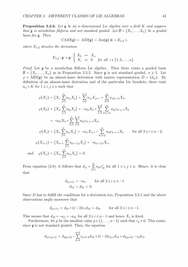
CHAPTER 3. DIFFERENT CLASSES OF LIE ALGEBRAS 43
Proposition 3.2.6. Let g be an n-dimensional Lie algebra over a field K and supposethat g is metabelian filiform and not standard graded. Let B = {X1, . . . ,Xn} be a gradedbasis for g. Then
CAID(g) = AID(g) = Inn(g) ⊕ < En,2 >,where En,2 denotes the derivation
En,2 ∶ g→ g ∶ { X2 ↦ Xn
Xi ↦ 0 for all i ∈ {1,3, . . . , n}.
Proof. Let g be a metabelian filiform Lie algebra. Then there exists a graded basisB = {X1, . . . ,Xn} as in Proposition 3.2.3. Since g is not standard graded, n ≥ 5. Letϕ ∈ AID(g) be an almost-inner derivation with matrix representation D = (dij). Bydefinition of an almost-inner derivation and of the particular Lie brackets, there existaij ∈K for 1 ≤ i, j ≤ n such that
ϕ(X1) = [X1,n
∑j=1
a1jXj] =n−1
∑j=2
a1jXj+1 =n
∑k=3
a1(k−1)Xk,
ϕ(X2) = [X2,n
∑j=1
a2jXj] = −a21X3 +n−2
∑j=3
n
∑k=j+2
a2jck−j−1Xk
= −a21X3 +n
∑k=5
k−2
∑j=3
a2jck−j−1Xk,
ϕ(Xi) = [Xi,n
∑j=1
aijXj] = −ai1Xi+1 −n
∑k=i+2
ai2ck−i−1Xk for all 3 ≤ i ≤ n − 2,
ϕ(Xn−1) = [Xn−1,n
∑j=1
a(n−1)jXj] = −a(n−1)1Xn,
and ϕ(Xn) = [Xn,n
∑j=1
anjXj] = 0.
From equation (2.8), it follows that dij =n
∑k=1
aikcjik for all 1 ≤ i, j ≤ n. Hence, it is clear
that
di(i+1) = −ai1 for all 2 ≤ i ≤ n − 1
d12 = d24 = 0.
Since D has to fulfill the conditions for a derivation too, Proposition 3.2.5 and the aboveobservations imply moreover that
di(i+1) = d23 + (i − 3)c1d12 = d23 for all 3 ≤ i ≤ n − 1.
This means that d23 = −ai1 = −a21 for all 3 ≤ i ≤ n − 1 and hence X1 is fixed.Furthermore, let p be the smallest value p ∈ {1, . . . , n−4} such that cp ≠ 0. This exists,
since g is not standard graded. Then, the equation
di(i+p+1) = d2(p+3) −p+2
∑k=3
cp+3−kd1k + (i − 3)cp+1d12 = d2(p+3) − cpd13
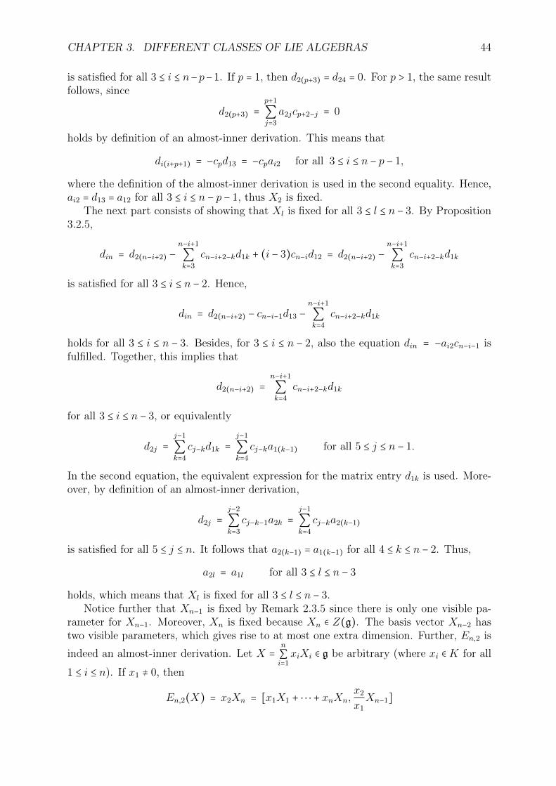
CHAPTER 3. DIFFERENT CLASSES OF LIE ALGEBRAS 44
is satisfied for all 3 ≤ i ≤ n−p−1. If p = 1, then d2(p+3) = d24 = 0. For p > 1, the same resultfollows, since
d2(p+3) =p+1
∑j=3
a2jcp+2−j = 0
holds by definition of an almost-inner derivation. This means that
di(i+p+1) = −cpd13 = −cpai2 for all 3 ≤ i ≤ n − p − 1,
where the definition of the almost-inner derivation is used in the second equality. Hence,ai2 = d13 = a12 for all 3 ≤ i ≤ n − p − 1, thus X2 is fixed.
The next part consists of showing that Xl is fixed for all 3 ≤ l ≤ n − 3. By Proposition3.2.5,
din = d2(n−i+2) −n−i+1
∑k=3
cn−i+2−kd1k + (i − 3)cn−id12 = d2(n−i+2) −n−i+1
∑k=3
cn−i+2−kd1k
is satisfied for all 3 ≤ i ≤ n − 2. Hence,
din = d2(n−i+2) − cn−i−1d13 −n−i+1
∑k=4
cn−i+2−kd1k
holds for all 3 ≤ i ≤ n − 3. Besides, for 3 ≤ i ≤ n − 2, also the equation din = −ai2cn−i−1 isfulfilled. Together, this implies that
d2(n−i+2) =n−i+1
∑k=4
cn−i+2−kd1k
for all 3 ≤ i ≤ n − 3, or equivalently
d2j =j−1
∑k=4
cj−kd1k =j−1
∑k=4
cj−ka1(k−1) for all 5 ≤ j ≤ n − 1.
In the second equation, the equivalent expression for the matrix entry d1k is used. More-over, by definition of an almost-inner derivation,
d2j =j−2
∑k=3
cj−k−1a2k =j−1
∑k=4
cj−ka2(k−1)
is satisfied for all 5 ≤ j ≤ n. It follows that a2(k−1) = a1(k−1) for all 4 ≤ k ≤ n − 2. Thus,
a2l = a1l for all 3 ≤ l ≤ n − 3
holds, which means that Xl is fixed for all 3 ≤ l ≤ n − 3.Notice further that Xn−1 is fixed by Remark 2.3.5 since there is only one visible pa-
rameter for Xn−1. Moreover, Xn is fixed because Xn ∈ Z(g). The basis vector Xn−2 hastwo visible parameters, which gives rise to at most one extra dimension. Further, En,2 is
indeed an almost-inner derivation. Let X =n
∑i=1xiXi ∈ g be arbitrary (where xi ∈ K for all
1 ≤ i ≤ n). If x1 ≠ 0, then
En,2(X) = x2Xn = [x1X1 + ⋅ ⋅ ⋅ + xnXn,x2x1Xn−1]
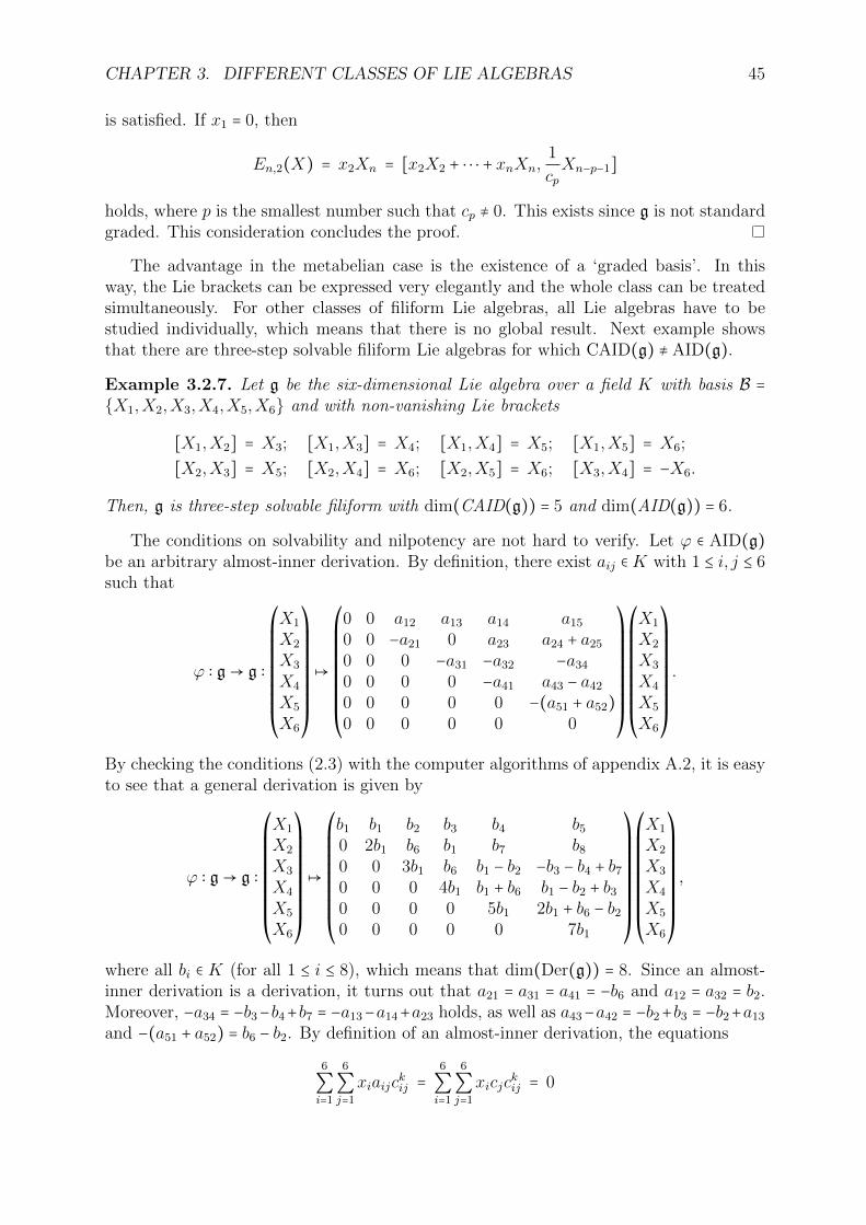
CHAPTER 3. DIFFERENT CLASSES OF LIE ALGEBRAS 45
is satisfied. If x1 = 0, then
En,2(X) = x2Xn = [x2X2 + ⋅ ⋅ ⋅ + xnXn,1
cpXn−p−1]
holds, where p is the smallest number such that cp ≠ 0. This exists since g is not standardgraded. This consideration concludes the proof.
The advantage in the metabelian case is the existence of a ‘graded basis’. In thisway, the Lie brackets can be expressed very elegantly and the whole class can be treatedsimultaneously. For other classes of filiform Lie algebras, all Lie algebras have to bestudied individually, which means that there is no global result. Next example showsthat there are three-step solvable filiform Lie algebras for which CAID(g) ≠ AID(g).
Example 3.2.7. Let g be the six-dimensional Lie algebra over a field K with basis B ={X1,X2,X3,X4,X5,X6} and with non-vanishing Lie brackets
[X1,X2] = X3; [X1,X3] = X4; [X1,X4] = X5; [X1,X5] = X6;
[X2,X3] = X5; [X2,X4] = X6; [X2,X5] = X6; [X3,X4] = −X6.
Then, g is three-step solvable filiform with dim(CAID(g)) = 5 and dim(AID(g)) = 6.
The conditions on solvability and nilpotency are not hard to verify. Let ϕ ∈ AID(g)be an arbitrary almost-inner derivation. By definition, there exist aij ∈K with 1 ≤ i, j ≤ 6such that
ϕ ∶ g→ g ∶
⎛⎜⎜⎜⎜⎜⎜⎜⎜⎜⎝
X1
X2
X3
X4
X5
X6
⎞⎟⎟⎟⎟⎟⎟⎟⎟⎟⎠
↦
⎛⎜⎜⎜⎜⎜⎜⎜⎜⎜⎝
0 0 a12 a13 a14 a150 0 −a21 0 a23 a24 + a250 0 0 −a31 −a32 −a340 0 0 0 −a41 a43 − a420 0 0 0 0 −(a51 + a52)0 0 0 0 0 0
⎞⎟⎟⎟⎟⎟⎟⎟⎟⎟⎠
⎛⎜⎜⎜⎜⎜⎜⎜⎜⎜⎝
X1
X2
X3
X4
X5
X6
⎞⎟⎟⎟⎟⎟⎟⎟⎟⎟⎠
.
By checking the conditions (2.3) with the computer algorithms of appendix A.2, it is easyto see that a general derivation is given by
ϕ ∶ g→ g ∶
⎛⎜⎜⎜⎜⎜⎜⎜⎜⎜⎝
X1
X2
X3
X4
X5
X6
⎞⎟⎟⎟⎟⎟⎟⎟⎟⎟⎠
↦
⎛⎜⎜⎜⎜⎜⎜⎜⎜⎜⎝
b1 b1 b2 b3 b4 b50 2b1 b6 b1 b7 b80 0 3b1 b6 b1 − b2 −b3 − b4 + b70 0 0 4b1 b1 + b6 b1 − b2 + b30 0 0 0 5b1 2b1 + b6 − b20 0 0 0 0 7b1
⎞⎟⎟⎟⎟⎟⎟⎟⎟⎟⎠
⎛⎜⎜⎜⎜⎜⎜⎜⎜⎜⎝
X1
X2
X3
X4
X5
X6
⎞⎟⎟⎟⎟⎟⎟⎟⎟⎟⎠
,
where all bi ∈ K (for all 1 ≤ i ≤ 8), which means that dim(Der(g)) = 8. Since an almost-inner derivation is a derivation, it turns out that a21 = a31 = a41 = −b6 and a12 = a32 = b2.Moreover, −a34 = −b3−b4+b7 = −a13−a14+a23 holds, as well as a43−a42 = −b2+b3 = −b2+a13and −(a51 + a52) = b6 − b2. By definition of an almost-inner derivation, the equations
6
∑i=1
6
∑j=1
xiaijckij =
6
∑i=1
6
∑j=1
xicjckij = 0
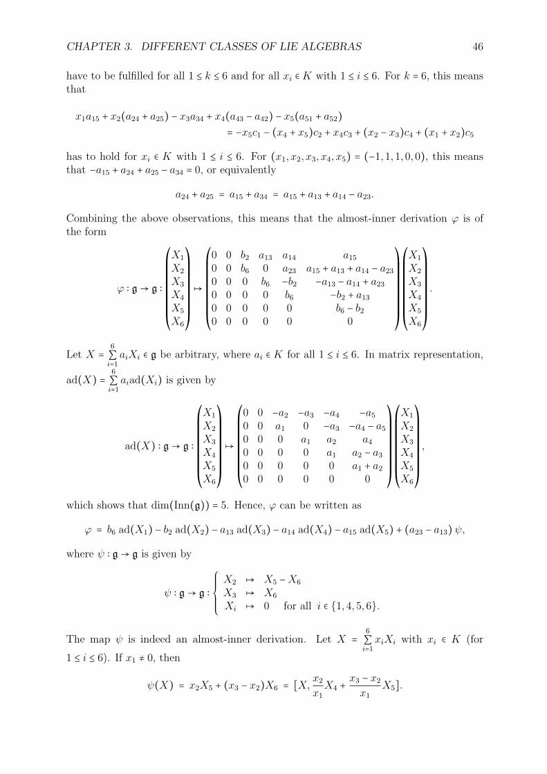
CHAPTER 3. DIFFERENT CLASSES OF LIE ALGEBRAS 46
have to be fulfilled for all 1 ≤ k ≤ 6 and for all xi ∈K with 1 ≤ i ≤ 6. For k = 6, this meansthat
x1a15 + x2(a24 + a25) − x3a34 + x4(a43 − a42) − x5(a51 + a52)= −x5c1 − (x4 + x5)c2 + x4c3 + (x2 − x3)c4 + (x1 + x2)c5
has to hold for xi ∈ K with 1 ≤ i ≤ 6. For (x1, x2, x3, x4, x5) = (−1,1,1,0,0), this meansthat −a15 + a24 + a25 − a34 = 0, or equivalently
a24 + a25 = a15 + a34 = a15 + a13 + a14 − a23.
Combining the above observations, this means that the almost-inner derivation ϕ is ofthe form
ϕ ∶ g→ g ∶
⎛⎜⎜⎜⎜⎜⎜⎜⎜⎜⎝
X1
X2
X3
X4
X5
X6
⎞⎟⎟⎟⎟⎟⎟⎟⎟⎟⎠
↦
⎛⎜⎜⎜⎜⎜⎜⎜⎜⎜⎝
0 0 b2 a13 a14 a150 0 b6 0 a23 a15 + a13 + a14 − a230 0 0 b6 −b2 −a13 − a14 + a230 0 0 0 b6 −b2 + a130 0 0 0 0 b6 − b20 0 0 0 0 0
⎞⎟⎟⎟⎟⎟⎟⎟⎟⎟⎠
⎛⎜⎜⎜⎜⎜⎜⎜⎜⎜⎝
X1
X2
X3
X4
X5
X6
⎞⎟⎟⎟⎟⎟⎟⎟⎟⎟⎠
.
Let X =6
∑i=1aiXi ∈ g be arbitrary, where ai ∈ K for all 1 ≤ i ≤ 6. In matrix representation,
ad(X) =6
∑i=1aiad(Xi) is given by
ad(X) ∶ g→ g ∶
⎛⎜⎜⎜⎜⎜⎜⎜⎜⎜⎝
X1
X2
X3
X4
X5
X6
⎞⎟⎟⎟⎟⎟⎟⎟⎟⎟⎠
↦
⎛⎜⎜⎜⎜⎜⎜⎜⎜⎜⎝
0 0 −a2 −a3 −a4 −a50 0 a1 0 −a3 −a4 − a50 0 0 a1 a2 a40 0 0 0 a1 a2 − a30 0 0 0 0 a1 + a20 0 0 0 0 0
⎞⎟⎟⎟⎟⎟⎟⎟⎟⎟⎠
⎛⎜⎜⎜⎜⎜⎜⎜⎜⎜⎝
X1
X2
X3
X4
X5
X6
⎞⎟⎟⎟⎟⎟⎟⎟⎟⎟⎠
,
which shows that dim(Inn(g)) = 5. Hence, ϕ can be written as
ϕ = b6 ad(X1) − b2 ad(X2) − a13 ad(X3) − a14 ad(X4) − a15 ad(X5) + (a23 − a13) ψ,
where ψ ∶ g→ g is given by
ψ ∶ g→ g ∶⎧⎪⎪⎪⎪⎨⎪⎪⎪⎪⎩
X2 ↦ X5 −X6
X3 ↦ X6
Xi ↦ 0 for all i ∈ {1,4,5,6}.
The map ψ is indeed an almost-inner derivation. Let X =6
∑i=1xiXi with xi ∈ K (for
1 ≤ i ≤ 6). If x1 ≠ 0, then
ψ(X) = x2X5 + (x3 − x2)X6 = [X, x2x1X4 +
x3 − x2x1
X5].
CHAPTER 3. DIFFERENT CLASSES OF LIE ALGEBRAS 47
Further,
ψ(X) = x2X5 + (x3 − x2)X6 = [6
∑i=2
xiXi,X3 −X4 −x4x2X5]
is satisfied if x1 = 0 and x2 ≠ 0. For x1 = x2 = 0,
ψ(X) = x3X6 = [6
∑i=3
xiXi,−X4]
holds. It is easy to see that ψ is not central almost-inner. For this Lie algebra,
Inn(g) = CAID(g) ⊊ AID(g) ⊊ Der(g)
is fulfilled. Hence, the result for metabelian filiform Lie algebras can not be generalisedto general filiform ones.
3.3 Two-step nilpotent Lie algebras determined by
graphs
There is a strong connection between finite simple graphs and some two-step nilpotentLie algebras. Let G(V,E) be a finite simple graph with vertices V = {X1, . . . ,Xn} andedges E. If there is an edge between Xi and Xj (with i < j), it is denoted with Yij. LetX be the vector space with basis the elements of V and let Y be the vector space withbasis the edges of E. The vector space g = X ⊕ Y can be viewed as a Lie algebra, wherethe brackets are given by
[Xi,Xj] =⎧⎪⎪⎪⎪⎨⎪⎪⎪⎪⎩
Yij if i < j and Yij ∈ E;−Yji if i > j and Yji ∈ E;
0 if there is no edge between Xi and Xj;
[Xi, Yjk] = 0 for all Xi ∈ V and for all Yjk ∈ E;
[Yij, Ykl] = 0 for all Yij, Ykl ∈ E.
It is easy to see that by construction, this defines a nilpotent Lie algebra with nilindextwo.
Conversely, an arbitrary nilpotent Lie algebra with nilindex two is determined by agraph when there exists a basis such that every basis vector appears at most once. It isnot always clear at first sight if this condition is satisfied.
Example 3.3.1. The two-step nilpotent Lie algebra g over a field K with basis B ={X1,X2,X3,X4} and Lie brackets
[X1,X2] = X4 and [X1,X3] = X4
can be determined by a graph.
Consider the basis B′ = {X1,X2,X ′
3,X4}, where X ′
3 =X3 −X2. It is not difficult to seethat for this new basis, the only non-zero Lie bracket is [X1,X2] = X4, since
[X1,X′
3] = [X1,X3] − [X1,X2] = 0.
This corresponds to a graph with three vertices (X1,X2 and X ′
3) and one edge (X4).However, not all two-step nilpotent Lie algebras can be formed in that way.
CHAPTER 3. DIFFERENT CLASSES OF LIE ALGEBRAS 48
Example 3.3.2. The two-step nilpotent Lie algebra g over a field K with basis B ={X1,X2,X3,X4,X5} and Lie brackets
[X1,X2] = X5 and [X3,X4] = X5
can not be determined by a graph.
In this example, it is easy to see that for every basis, there exists a basis vector whichappears twice.
For two-step nilpotent Lie algebras determined by graphs, there exists a global resultabout the almost-inner derivations.
Proposition 3.3.3. Let g be a two-step nilpotent Lie algebra determined by a graph.Then all almost-inner derivations of g are inner.
Proof. Let G(V,E) be the simple graph corresponding to g. Then g can be written asg = X ⊕ Y , where X is the vector space with basis the elements of V and Y the vectorspace with basis the edges of E. Denote the dimension of g with n. Let ϕ be an arbitraryalmost-inner derivation of g with parameters aij, where 1 ≤ i, j ≤ n. It is enough to showthat all basis vectors are fixed. The basis elements of Y belong to the centre of g and arehence fixed. By Remark 2.3.5, it suffices to consider the basis vectors Xi of X with morethan one visible parameter. Let Xi ∈ X be an arbitrary basis element with at least twovisible parameters. Choose j, k, l and m arbitrarily in {1, . . . , n} so that ckij ≠ 0 ≠ cmil andj ≠ l. This means that aji and ali are visible parameters belonging to Xi. By construction,k and m have to be different, since every edge belongs to exactly two vertices. By thesame reasoning, Xk and Xm appear once. Hence, the conditions for Lemma 2.3.8 arefulfilled for (i, j, k, l,m), which shows that aji = ali. Since j, k, l and m were arbitrary, thismeans that Xi has to be fixed. Therefore, all basis vectors of g are fixed. Lemma 2.3.6concludes the proof.
Note that the converse of this proposition does not hold. Indeed, for the Lie algebrafrom Example 3.3.2, all almost-inner derivations are inner. This immediately follows fromequation (2.10), since dim(Inn(g)) = 4 and
5
∑i=1
di = 1 + 1 + 1 + 1 + 0 = 4,
where di is as in Definition 2.3.3.The result of the previous proposition can not be generalised for two-step nilpotent
Lie algebras.
Example 3.3.4. Let g be the six-dimensional Lie algebra over a field K with basis B ={X1,X2,X3,X4,X5,X6} and Lie brackets defined by
[X1,X2] = X5, [X1,X3] = X6 and [X3,X4] = X5.
Then, g is two-step nilpotent with
dim(AID(g)Inn(g) ) = 6 − 4 = 2.
CHAPTER 3. DIFFERENT CLASSES OF LIE ALGEBRAS 49
Analogously as in Example 3.3.2, the Lie algebra g can not be determined by a graph.Remark first that six is an upper bound for the dimension of the almost-inner derivations,
sincen
∑i=1di = 2 + 1 + 2 + 1 + 0 + 0 = 6. The derivation ϕ1 ∶ g→ g defined as
ϕ1 ∶ g→ g ∶ { X1 ↦ X6
Xi ↦ 0 for all i ∈ {2, . . . ,6}
is almost-inner. Let X =6
∑i=1xiXi with xi ∈K (for 1 ≤ i ≤ 6). The definition is automatically
satisfied when x1 = 0. If x1 ≠ 0, then
ϕ1(X) = x1X6 = x4X5 + x1X6 − x4X5 = [X, x4x1X2 +X3].
Further, the derivation
ϕ2 ∶ g→ g ∶ { X3 ↦ X6
Xi ↦ 0 for all i ∈ {1,2,4,5,6}
is almost-inner. Consider X =6
∑i=1xiXi with xi ∈ K (for 1 ≤ i ≤ 6). When x3 = 0, the
definition is immediately satisfied. If x3 ≠ 0, then
ϕ2(X) = x3X6 = x2X5 + x3X6 − x2X5 = [X,−X1 −x2x3X4]
holds. It is easy to see that no linear combination of ϕ1 and ϕ2 belongs to Inn(g).Moreover, due to Proposition 2.3.10, it is possible to construct a Lie algebra g for
which
dim(AID(g)Inn(g) )
is arbitrary large. However, CAID(g) = AID(g) will always hold when g is two-stepnilpotent Lie algebra, by Lemma 2.1.10.
3.4 Free nilpotent Lie algebras
Section 3.2 was about filiform Lie algebras, the so-called ‘less’ nilpotent Lie algebras.Then, a special case of the ‘most’ (non-abelian) nilpotent Lie algebras were treated. Thenext class consists of the free nilpotent Lie algebras, where all nilindices can occur. First,the notion of a free Lie algebra is explained and a suitable basis is worked out. Further,for free nilpotent Lie algebras with nilindex is equal to two or three, results concerningthe almost-inner derivations are proven.
As is the case for groups, a Lie algebra can be free too.
Definition 3.4.1 (Free Lie algebra). Let X be a set and g a Lie algebra. Let i ∶ X → gbe a set map. The Lie algebra g is free on X if for every Lie algebra g with a set mapf ∶X → g, there is a unique Lie algebra morphism ϕ ∶ g→ g with f = ϕ ○ i.
One can show that for every set X, there is a unique free Lie algebra generated by X.This Lie algebra has M ∶= ∣X ∣ generators and is denoted with gM . By definition, the onlyrelations for free Lie algebras are due to the skew-symmetry and the Jacobi-identity.
CHAPTER 3. DIFFERENT CLASSES OF LIE ALGEBRAS 50
Definition 3.4.2 (Length of a generator). Let gM be a free Lie algebra with M generators.The length d of a generator Xi (with 1 ≤ i ≤M) is defined as d(Xi) = 1. The length of aLie bracket in the generators is defined recursively as
d([X,Y ]) = d(X) + d(Y ) where X,Y ∈ gM and X ≠ 0 ≠ Y.
Moreover, d(0) = 0 holds.
As an example, consider g5, the free Lie algebra on 5 generators. Then d(X2) = 1 andd([X3,X4]) = 2, which shows that d([X2, [X3,X4]]) = 3. This implies that
d([X3,X5], [X2, [X3,X4]]) = 5.
Note that d([X2, [[X1,X3], [X1,X3]]]) = 0, since [[X1,X3], [X1,X3]] = 0. Let X ∈ gMand X ≠ 0, then X can be written as Lie bracket in the generators. The length of X canmore or less be seen as the number of generators which are used in this expression. Thelength of a Lie bracket is used in the definition of a Hall set.
Definition 3.4.3 (Hall set). Let gM be a free Lie algebra with M generators. Then a setBM = {X1,X2, . . .} is called a Hall set for gM when it satisfies the following conditions:
• The first M elements are the generators X1, . . .XM ;
• If i and j are positive integers so that d(Xi) < d(Xj), then i < j holds;
• Let Xi,Xj ∈ gM , then [Xi,Xj] ∈ BM if and only if both Xi,Xj ∈ BM , the inequalityi < j holds and either Xj is a generator, or Xj = [Xl,Xm] for some Xl,Xm ∈ BMwith l ≤ i.
Consider the free Lie algebra with three generators. Then A ∶= [X1, [X1,X3]] ∈ B3 andB ∶= [X2, [X1,X3]] ∈ B3, but [X1, [X2,X3]] ∉ B3. Since A,B ∈ B, they can be written asA ∶= Xa respectively B ∶= Xb, where a, b ∈ N. However, there is no fixed rule to decidewhether a < b or b < a. Of course, the Hall set depends on the choice or ordering. LetXm1 ,Xm2 ∈ B3 with m1 ≠m2 and suppose that
Xm1 ∶= [Xi,Xj] and Xm2 ∶= [Xk,Xl],
where Xi,Xj,Xk,Xl ∈ B3. In this thesis, the convention is used that the relation
m1 <m2 if and only if (i < k) or (i = k and j < l)
holds. It turns out that the Hall set can be used as a basis for a free Lie algebra.
Theorem 3.4.4. Let gM be a free Lie algebra with M generators. A Hall set for gMdefines a basis for gM .
Proof. A proof of this fact is given in [5, chapter 7].
This basis has infinitely many elements. A related notion is that of a free nilpotentLie algebra.
Definition 3.4.5 (Free nilpotent Lie algebra). The free nilpotent Lie algebra gM,r withM generators and with nilindex r is the quotient of the free Lie algebra with M generatorsby the ideal gr+1.
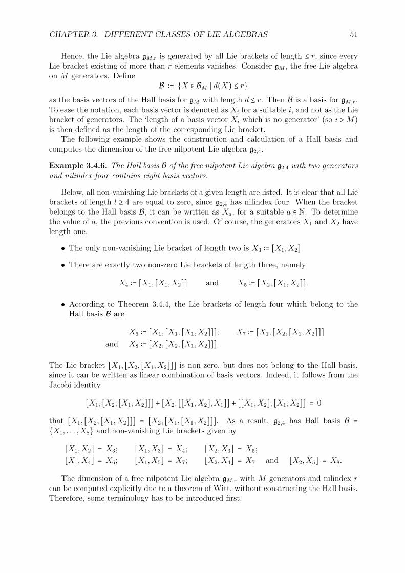
CHAPTER 3. DIFFERENT CLASSES OF LIE ALGEBRAS 51
Hence, the Lie algebra gM,r is generated by all Lie brackets of length ≤ r, since everyLie bracket existing of more than r elements vanishes. Consider gM , the free Lie algebraon M generators. Define
B ∶= {X ∈ BM ∣ d(X) ≤ r}as the basis vectors of the Hall basis for gM with length d ≤ r. Then B is a basis for gM,r.To ease the notation, each basis vector is denoted as Xi for a suitable i, and not as the Liebracket of generators. The ‘length of a basis vector Xi which is no generator’ (so i >M)is then defined as the length of the corresponding Lie bracket.
The following example shows the construction and calculation of a Hall basis andcomputes the dimension of the free nilpotent Lie algebra g2,4.
Example 3.4.6. The Hall basis B of the free nilpotent Lie algebra g2,4 with two generatorsand nilindex four contains eight basis vectors.
Below, all non-vanishing Lie brackets of a given length are listed. It is clear that all Liebrackets of length l ≥ 4 are equal to zero, since g2,4 has nilindex four. When the bracketbelongs to the Hall basis B, it can be written as Xa, for a suitable a ∈ N. To determinethe value of a, the previous convention is used. Of course, the generators X1 and X2 havelength one.
• The only non-vanishing Lie bracket of length two is X3 ∶= [X1,X2].
• There are exactly two non-zero Lie brackets of length three, namely
X4 ∶= [X1, [X1,X2]] and X5 ∶= [X2, [X1,X2]].
• According to Theorem 3.4.4, the Lie brackets of length four which belong to theHall basis B are
X6 ∶= [X1, [X1, [X1,X2]]]; X7 ∶= [X1, [X2, [X1,X2]]]and X8 ∶= [X2, [X2, [X1,X2]]].
The Lie bracket [X1, [X2, [X1,X2]]] is non-zero, but does not belong to the Hall basis,since it can be written as linear combination of basis vectors. Indeed, it follows from theJacobi identity
[X1, [X2, [X1,X2]]] + [X2, [[X1,X2],X1]] + [[X1,X2], [X1,X2]] = 0
that [X1, [X2, [X1,X2]]] = [X2, [X1, [X1,X2]]]. As a result, g2,4 has Hall basis B ={X1, . . . ,X8} and non-vanishing Lie brackets given by
[X1,X2] = X3; [X1,X3] = X4; [X2,X3] = X5;
[X1,X4] = X6; [X1,X5] = X7; [X2,X4] = X7 and [X2,X5] = X8.
The dimension of a free nilpotent Lie algebra gM,r with M generators and nilindex rcan be computed explicitly due to a theorem of Witt, without constructing the Hall basis.Therefore, some terminology has to be introduced first.
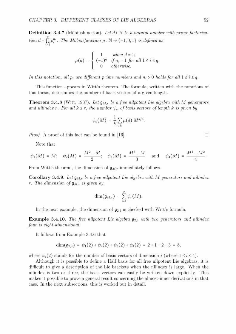
CHAPTER 3. DIFFERENT CLASSES OF LIE ALGEBRAS 52
Definition 3.4.7 (Mobiusfunction). Let d ∈ N be a natural number with prime factorisa-
tion d =q
∏i=1pnii . The Mobiusfunction µ ∶ N→ {−1,0,1} is defined as
µ(d) =⎧⎪⎪⎪⎪⎨⎪⎪⎪⎪⎩
1 when d = 1;(−1)q if ni = 1 for all 1 ≤ i ≤ q;
0 otherwise.
In this notation, all pi are different prime numbers and ni > 0 holds for all 1 ≤ i ≤ q.
This function appears in Witt’s theorem. The formula, written with the notations ofthis thesis, determines the number of basis vectors of a given length.
Theorem 3.4.8 (Witt, 1937). Let gM,r be a free nilpotent Lie algebra with M generatorsand nilindex r. For all k ≤ r, the number ψk of basis vectors of length k is given by
ψk(M) = 1
k∑d∣k
µ(d)Mk/d.
Proof. A proof of this fact can be found in [16].
Note that
ψ1(M) = M ; ψ2(M) = M2 −M2
; ψ3(M) = M3 −M3
and ψ4(M) = M4 −M2
4.
From Witt’s theorem, the dimension of gM,r immediately follows.
Corollary 3.4.9. Let gM,r be a free nilpotent Lie algebra with M generators and nilindexr. The dimension of gM,r is given by
dim(gM,r) =r
∑i=1
ψr(M).
In the next example, the dimension of g2,4 is checked with Witt’s formula.
Example 3.4.10. The free nilpotent Lie algebra g2,4 with two generators and nilindexfour is eight-dimensional.
It follows from Example 3.4.6 that
dim(g2,4) = ψ1(2) + ψ2(2) + ψ3(2) + ψ4(2) = 2 + 1 + 2 + 3 = 8,
where ψi(2) stands for the number of basis vectors of dimension i (where 1 ≤ i ≤ 4).Although it is possible to define a Hall basis for all free nilpotent Lie algebras, it is
difficult to give a description of the Lie brackets when the nilindex is large. When thenilindex is two or three, the basis vectors can easily be written down explicitly. Thismakes it possible to prove a general result concerning the almost-inner derivations in thatcase. In the next subsections, this is worked out in detail.
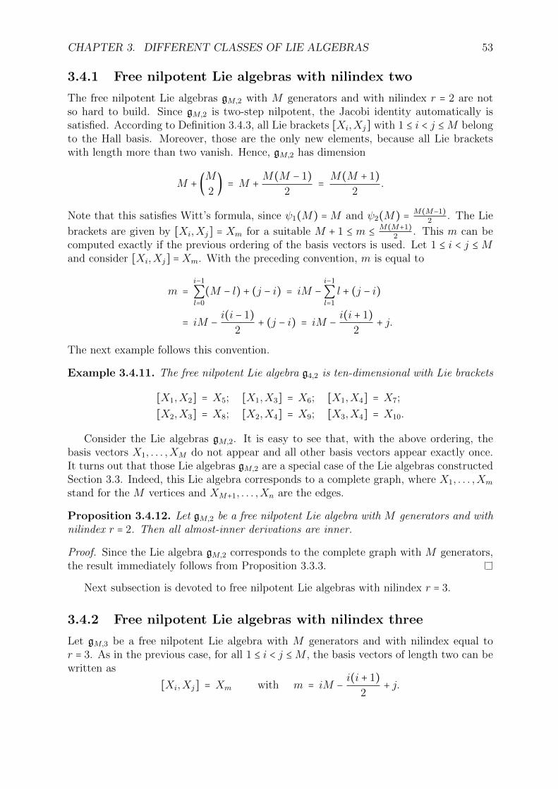
CHAPTER 3. DIFFERENT CLASSES OF LIE ALGEBRAS 53
3.4.1 Free nilpotent Lie algebras with nilindex two
The free nilpotent Lie algebras gM,2 with M generators and with nilindex r = 2 are notso hard to build. Since gM,2 is two-step nilpotent, the Jacobi identity automatically issatisfied. According to Definition 3.4.3, all Lie brackets [Xi,Xj] with 1 ≤ i < j ≤M belongto the Hall basis. Moreover, those are the only new elements, because all Lie bracketswith length more than two vanish. Hence, gM,2 has dimension
M + (M2) = M + M(M − 1)
2= M(M + 1)
2.
Note that this satisfies Witt’s formula, since ψ1(M) =M and ψ2(M) = M(M−1)2 . The Lie
brackets are given by [Xi,Xj] = Xm for a suitable M + 1 ≤ m ≤ M(M+1)2 . This m can be
computed exactly if the previous ordering of the basis vectors is used. Let 1 ≤ i < j ≤Mand consider [Xi,Xj] =Xm. With the preceding convention, m is equal to
m =i−1
∑l=0
(M − l) + (j − i) = iM −i−1
∑l=1
l + (j − i)
= iM − i(i − 1)2
+ (j − i) = iM − i(i + 1)2
+ j.
The next example follows this convention.
Example 3.4.11. The free nilpotent Lie algebra g4,2 is ten-dimensional with Lie brackets
[X1,X2] = X5; [X1,X3] = X6; [X1,X4] = X7;
[X2,X3] = X8; [X2,X4] = X9; [X3,X4] = X10.
Consider the Lie algebras gM,2. It is easy to see that, with the above ordering, thebasis vectors X1, . . . ,XM do not appear and all other basis vectors appear exactly once.It turns out that those Lie algebras gM,2 are a special case of the Lie algebras constructedSection 3.3. Indeed, this Lie algebra corresponds to a complete graph, where X1, . . . ,Xm
stand for the M vertices and XM+1, . . . ,Xn are the edges.
Proposition 3.4.12. Let gM,2 be a free nilpotent Lie algebra with M generators and withnilindex r = 2. Then all almost-inner derivations are inner.
Proof. Since the Lie algebra gM,2 corresponds to the complete graph with M generators,the result immediately follows from Proposition 3.3.3.
Next subsection is devoted to free nilpotent Lie algebras with nilindex r = 3.
3.4.2 Free nilpotent Lie algebras with nilindex three
Let gM,3 be a free nilpotent Lie algebra with M generators and with nilindex equal tor = 3. As in the previous case, for all 1 ≤ i < j ≤M , the basis vectors of length two can bewritten as
[Xi,Xj] = Xm with m = iM − i(i + 1)2
+ j.
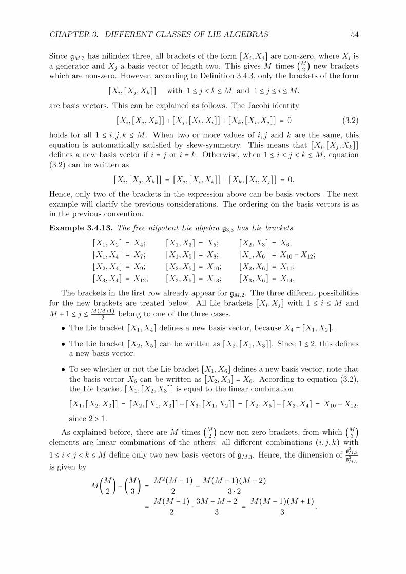
CHAPTER 3. DIFFERENT CLASSES OF LIE ALGEBRAS 54
Since gM,3 has nilindex three, all brackets of the form [Xi,Xj] are non-zero, where Xi isa generator and Xj a basis vector of length two. This gives M times (M
2) new brackets
which are non-zero. However, according to Definition 3.4.3, only the brackets of the form
[Xi, [Xj,Xk]] with 1 ≤ j < k ≤M and 1 ≤ j ≤ i ≤M.
are basis vectors. This can be explained as follows. The Jacobi identity
[Xi, [Xj,Xk]] + [Xj, [Xk,Xi]] + [Xk, [Xi,Xj]] = 0 (3.2)
holds for all 1 ≤ i, j, k ≤ M . When two or more values of i, j and k are the same, thisequation is automatically satisfied by skew-symmetry. This means that [Xi, [Xj,Xk]]defines a new basis vector if i = j or i = k. Otherwise, when 1 ≤ i < j < k ≤ M , equation(3.2) can be written as
[Xi, [Xj,Xk]] = [Xj, [Xi,Xk]] − [Xk, [Xi,Xj]] = 0.
Hence, only two of the brackets in the expression above can be basis vectors. The nextexample will clarify the previous considerations. The ordering on the basis vectors is asin the previous convention.
Example 3.4.13. The free nilpotent Lie algebra g3,3 has Lie brackets
[X1,X2] = X4; [X1,X3] = X5; [X2,X3] = X6;
[X1,X4] = X7; [X1,X5] = X8; [X1,X6] = X10 −X12;
[X2,X4] = X9; [X2,X5] = X10; [X2,X6] = X11;
[X3,X4] = X12; [X3,X5] = X13; [X3,X6] = X14.
The brackets in the first row already appear for gM,2. The three different possibilitiesfor the new brackets are treated below. All Lie brackets [Xi,Xj] with 1 ≤ i ≤ M and
M + 1 ≤ j ≤ M(M+1)2 belong to one of the three cases.
• The Lie bracket [X1,X4] defines a new basis vector, because X4 = [X1,X2].
• The Lie bracket [X2,X5] can be written as [X2, [X1,X3]]. Since 1 ≤ 2, this definesa new basis vector.
• To see whether or not the Lie bracket [X1,X6] defines a new basis vector, note thatthe basis vector X6 can be written as [X2,X3] = X6. According to equation (3.2),the Lie bracket [X1, [X2,X3]] is equal to the linear combination
[X1, [X2,X3]] = [X2, [X1,X3]] − [X3, [X1,X2]] = [X2,X5] − [X3,X4] = X10 −X12,
since 2 > 1.
As explained before, there are M times (M2) new non-zero brackets, from which (M
3)
elements are linear combinations of the others: all different combinations (i, j, k) with
1 ≤ i < j < k ≤M define only two new basis vectors of gM,3. Hence, the dimension ofg3M,3
g2M,3
is given by
M(M2) − (M
3) = M2(M − 1)
2− M(M − 1)(M − 2)
3 ⋅ 2
= M(M − 1)2
⋅ 3M −M + 2
3= M(M − 1)(M + 1)
3.
CHAPTER 3. DIFFERENT CLASSES OF LIE ALGEBRAS 55
When M = 2, the dimension ofg32,3g22,3
is equal to M(M2) = 2 = M(M−1)(M+1)
3 . Hence, the
formula for the dimension remains valid. Note that ψ3(M) = M(M2−1)
3 , which is an appli-cation of Witt’s formula. This implies that the dimension of gM,3 is
M + M(M − 1)2
+ M(M − 1)(M + 1)3
= M (6 + 3(M − 1) + 2(M2 − 1)6
)
= M (2M2 + 3M + 1
6) .
As an example, the dimension of g3,3 is given by
M (2M2 + 3M + 1
6) = 3(2 ⋅ 32 + 3 ⋅ 3 + 1
6) = 14.
Consider the Lie algebras gM,3. With the above convention, the basis vectors X1, . . . ,XM
do not appear. Further, the basis vectors of length two appear once. Let Xp a basis vectorof length three, so Xp = [Xj,Xs] where Xj is a generator and Xs can be written as Liebracket of two generators, say Xs = [Xi,Xk]. When 1 ≤ i < j ≠ k ≤ n, then Xp appearstwice, namely for {Xj,Xs} and also for {Xi,Xt}, where
Xt = [Xj,Xk] (if j < k) or Xt = [Xk,Xj] (if k < j).
Otherwise, Xp appears only once.
Remark 3.4.14. Let gM,3 be a free nilpotent Lie algebra with M generators and nilindexthree. Denote the Hall basis with B = {X1, . . . ,Xn}. The observations from before showthat if Xk appears twice, say for {Xi,Xj} and {Xa,Xb}, then a, b, i and l are pairwisedifferent.
Next proposition shows that AID(gM,3) = Inn(gM,3) for all possible values of M .
Proposition 3.4.15. Let gM,3 be a free nilpotent Lie algebra with M generators andnilindex r = 3. Then all almost-inner derivations are inner.
Proof. Denote n for the dimension of gM,3. Let ϕ ∈ AID(gM,3) with parameters aij (where1 ≤ i, j ≤ n). Choose Xi arbitrarily (where 1 ≤ i ≤ n). By Lemma 2.3.6, it suffices to showthat Xi is fixed. This is satisfied when all visible parameters belonging to Xi are equal.Let (j, k, l,m) ∈ {1, . . . , n}4 be arbitrary values such that ckij ≠ 0 and cmil ≠ 0, so aji and aliare visible parameters belonging to Xi. It follows from Remark 3.4.14 that k ≠ m. It isenough to prove that aji = ali. This is done in different steps.
• Consider first that the basis vector Xi is a generator. Choose 1 ≤ b ≤ M andM + 1 ≤ r ≤ n so that
crib ≠ 0 and ckbp = 0 = cmbp for all 1 ≤ p ≤ n
holds. This is always possible when Xk and Xm appear just once. When the basisvector Xk appears twice, then Xk has length three and there is one other generatorXa such that ckas ≠ 0, for a suitable s. Therefore, a is excluded in the choice for b.The same reasoning also holds when Xm appears twice. Hence, for M > 3, there are
CHAPTER 3. DIFFERENT CLASSES OF LIE ALGEBRAS 56
thus at least M − 3 possible choices for b, note that b cannot be equal to i. WhenM = 2, there are no basis vectors which appear twice; for M = 3, there are only twobasis vectors which appear twice. It is clear from Example 3.4.13 that those vectorscannot be both Xk and Xm. This means that the values 1 ≤ b ≤ M and 1 ≤ r ≤ nalso can be found in these cases. Further, ckpj = cmpl = 0 for all 1 ≤ p ≤ n with p ≠ iholds by Remark 3.4.14. Moreover, the basis vector Xr appears once, since it haslength two. Therefore,
crqb = 0 for all 1 ≤ q ≤ n with q ≠ iand crpj = crpl = 0 for all 1 ≤ q ≤ n
hold. Lemma 2.3.8 can be used with (i, j, k, b, r) respectively (i, l,m, b, r), whichshows that aji = abi respectively ali = abi. Together, this implies that aji = ali, whichwas to show.
• Suppose now that Xi is not a generator. If Xi ∉ Z(gM,3), it is automatically fixed.Otherwise, there exists a unique pair 1 ≤ a < b ≤ M so that [Xa,Xb] = Xi. DenoteXs and Xt for the basis vectors Xs = [Xa,Xi] respectively Xt = [Xb,Xi]. Byconstruction, Xs and Xt appear once. Hence, it follows from Lemma 2.3.8 with(i, a, s, b, t) that aai = abi. The rest of the proof goes in two different steps.
– When ckap = 0 for all 1 ≤ p ≤ n, Lemma 2.3.8 can be used with (i, j, k, a, s), whichshows that aji = aai. Otherwise, since Xk appears at most twice, the equationckbp = 0 is satisfied for all 1 ≤ p ≤ n. Hence, Lemma 2.3.8 with (i, j, k, b, t) impliesthat aji = abi.
– If clap = 0 holds for all 1 ≤ p ≤ n, it follows from Lemma 2.3.8 with (i, l,m, a, s)that ali = aai. If this is not the case, cmbp = 0 holds for all 1 ≤ p ≤ n, since thebasis vector Xm appears at most twice. Lemma 2.3.8 with (i, l,m, b, t) thengives that ali = abi.
Since aai = abi, the above observations show that aji = ali.
In both cases, aji = ali is satisfied. Since aji and ali were two arbitrary visible parametersbelonging to Xi, the basis vector Xi is fixed. This finishes the proof.
The different cases in the proof of the proposition will be clarified with an example.
Example 3.4.16. For the fourteen-dimensional free nilpotent Lie algebra g3,3, it followsthat Inn(g3,3) = AID(g3,3).
The Lie brackets for this Lie algebra are listed in Example 3.4.13. Let ϕ ∈ AID(g3,3)be an almost-inner derivation with parameters aij (where 1 ≤ i, j ≤ 14).
• Consider the inequalities c924 ≠ 0 and c1025 ≠ 0. The way to show that a42 = a52 iswritten down in the first part of the proof, since X2 is a generator. Consider theLie brackets
[X2,X4] = [X2, [X1,X2]] = X9 and [X2,X5] = [X2, [X1,X3]] = X10.
The basis vector X9 appears once, but X10 appear twice. Indeed, the equationc1016 = 1 holds. Thus, b cannot be equal to one or two, which means that b = 3 is the
CHAPTER 3. DIFFERENT CLASSES OF LIE ALGEBRAS 57
only possibility (and r = 6). Further, the basis vector X6 = [X2,X3] appears onlyonce. Hence, Lemma 2.3.8 with (i, j, k, l,m) = (2,4,9,3,6) shows that a42 = a32.Moreover, it follows from the same lemma with (i, j, k, l,m) = (2,5,10,3,6) thata52 = a32. Those equations imply that a52 = a42.
• Consider the inequalities c1061 ≠ 0 and c1162 ≠ 0. The corresponding visible parametersa16 and a26 belong to X6, which can be written as X6 = [X2,X3]. Further, the basisvectors X11 = [X2,X6] and X14 = [X3,X6] appear once, so (a, b, s, t) = (2,3,11,14).Lemma 2.3.8 with (6,2,11,3,14) shows that a26 = a36. Further, c102p ≠ 0 holds forp = 5, but c103p = 0 is satisfied for all 1 ≤ p ≤ 14. Lemma 2.3.8 can be used with(i, j, k, l,m) = (6,1,10,3,14) to show that a16 = a36. Next, c1126 = 1, but c113p = 0 holdsfor all 1 ≤ p ≤ n, since X11 appears only once. It follows from Lemma 2.3.8 with(i, j, k, l,m) = (6,2,11,3,14) that a26 = a36. Both observations together give thedesired a16 = a26.
All other cases are analogous. Of course, in the last example, it can already be derivedthat a16 = a26 without the last step. However, the example is worked out completely toillustrate that the procedure is valid whether or not one or both of the values j and l areequal to a or b in the proof of the proposition.
Let gM,r be a free nilpotent Lie algebra with M generators and nilindex r > 3. It isstill possible to build a Hall basis and to determine the number of basis vectors. However,it becomes difficult to describe the relations between the basis vectors and hence the Liebrackets, since there are a lot of different cases which have to be treated. Therefore, it ishard to compute AID(gM,r), since the first step in the procedure mentioned in Subsection2.3.1 cannot be executed. Hence, there is no general result known concerning the almost-inner derivations of free nilpotent Lie algebras gM,r with M generators and nilindex r > 3.
3.5 Triangular matrices
This section is devoted to the study of the set of all strictly uppertriangular matrices andthe set of all uppertriangular matrices. It will turn out that those two subsets of gl(n,K)are in fact Lie subalgebras. First, some notation is introduced. Fix an n ∈ N and a fieldK. Consider gl(n,K), the Lie algebra of all (n×n)-matrices over the field K, introducedin Example 1.2.6. The matrix Eij is defined as
(Eij)k,l = { 1 if (k, l) = (i, j);0 otherwise.
It is clear that Bn = {Eij ∈Kn×n ∣ 1 ≤ i, j ≤ n} forms a basis of gl(n,K). Further, the Liebrackets are given by
[Eij,Ekl] = δjkEil − δliEkj.Next subsections describe the definition and the almost-inner derivations for the Lie al-gebras of (strictly) uppertriangular matrices. Of course, all properties obtained for theseclasses of Lie algebras also hold for the Lie algebras of all (strictly) lowertriangular ma-trices.
CHAPTER 3. DIFFERENT CLASSES OF LIE ALGEBRAS 58
3.5.1 Strictly uppertriangular matrices
The notation nn(K) ⊂ gl(n,K) stands for the set of all strictly uppertriangular (n × n)-matrices over the field K. Throughout this section, it will be assumed that n ≥ 2, sincen1(K) only contains zero. A basis for the vector space nn(K) is given by
Bn = {Eij ∈Kn×n ∣ 1 ≤ i < j ≤ n}.
Choose 1 ≤ i < j ≤ n and 1 ≤ k < l ≤ n arbitrarily. Since
[Eij,Ekl] = δjkEil − δliEkj
holds, the Lie bracket of two strictly uppertriangular matrices is again strictly uppertri-angular. Hence, nn(K) is a Lie subalgebra of gl(n,K). From the basis of nn(K), it isclear that the dimension of this Lie algebra is
dim(nn(K)) = n(n − 1)2
.
The Lie algebra n2(K) ≅ K is abelian. When n > 2, the Lie algebra nn(K) is nilpotentwith nilindex n − 1.
Example 3.5.1. The Lie algebra n3(K) over the field K is three-dimensional and hasB = {E12,E23,E13} as basis. The only non-zero Lie bracket is [E12,E23] = E13. This isthe standard graded filiform Lie algebra of dimension n = 3.
In the next lemma, the dimension of the Lie algebra of inner derivations of nn(K) isdetermined.
Lemma 3.5.2. Let nn(K) be the Lie algebra of all strictly uppertriangular (n×n)-matricesover the field K. When n > 1, it follows that
dim(Inn(nn(K))) = dim(nn(K)) − 1 = n2 − n − 2
2.
Proof. The dimension of Inn(nn(K)) is equal to the dimension of
vct{ad(Eij) ∶ nn(K)→ nn(K) ∣ 1 ≤ i < j ≤ n}.
Remark first that E1n belongs to the centre of nn(K), which shows the result for n = 2.Further, when n > 2, all inner derivations ad(Eij) ∶ nn(K)→ nn(K) are linear independentwhen 1 ≤ i < j ≤ n and (i, j) ≠ (1, n). Indeed, for all 1 ≤ j < k < n, the only inner derivationof a basis vector which maps Ekn to (a non-zero multiple of) Ejn is ad(Ejk). Further,ad(Ejn) is the only adjoint map belonging to a basis vector which maps E1j to (a non-zeromultiple of) −E1n, where 1 < j < n. This completes the proof.
Next proposition shows that the only almost-inner derivations for nn(K) are the innerones. The proof is based on the fact that an almost-inner derivation also satisfies theconditions for an arbitrary derivation.
Proposition 3.5.3. Let nn(K) be the Lie algebra of all strictly uppertriangular (n × n)-matrices over the field K. Then all almost-inner derivations are inner derivations.
CHAPTER 3. DIFFERENT CLASSES OF LIE ALGEBRAS 59
Proof. An abelian Lie algebra does not admit inner derivation, which shows the resultfor n = 2. When n = 3, the result immediately follows from Proposition 3.2.4. Supposenow that n > 3. Let ϕ ∈ AID(nn(K)) be an almost-inner derivation of nn(K). Then thereexist parameters aklij with 1 ≤ i, j, k, l ≤ n such that
ϕ(E1i) =n
∑t=i+1
ait1iE1t with 1 < i < n;
ϕ(E1n) = 0;
ϕ(Ejk) =j−1
∑t=1
−atjjkEtk +n
∑t=k+1
aktjkEjt with 1 < j < k < n;
ϕ(Ejn) =j−1
∑t=1
−atjjnEtn with 1 < j < n.
To enlarge the readability, the second index of the parameters is now written as a super-script. By Lemma 2.3.6, it suffices to show that all basis vectors are fixed. This goes indifferent steps.
• Remark that E1n belongs to the centre and is hence fixed by Remark 2.3.5.
• Choose E1i arbitrarily with 1 < i < n. The visible parameters belonging to E1i area1iij (with i < j ≤ n). When i = n − 1, there is only one visible parameter, namely
a1,n−1n−1,n. Hence, E1,n−1 is fixed by Remark 2.3.5. Otherwise, let i < j < n be arbitrary.By definition of the Lie brackets and of an arbitrary almost-inner derivation,
ϕ([Eij,Ejn]) = ϕ(Ein) =i−1
∑t=1
−atiinEtn
holds. Moreover, ϕ is a derivation and therefore,
ϕ([Eij,Ejn]) = [ϕ(Eij),Ejn] + [Eij, ϕ(Ejn)]
= [i−1
∑t=1
−atiijEtj +n
∑t=j+1
ajtijEit,Ejn] + [Eij,j−1
∑t=1
−atjjnEtn]
=i−1
∑t=1
−atiijEtn
has to be satisfied. Combining both equations leads to the following result:
atiin = atiij where 1 ≤ t < i < j < n.
In particular, this shows that for t = 1, all visible parameters belonging to E1i arethe same, thus E1i is fixed.
• Consider an arbitrary basis vector Ejk, where 1 < j < k < n. The visible parametersbelonging to Ejk are
ajkij and ajkkl , with 1 ≤ i < j < k < l ≤ n,
because the Lie brackets [Eij,Ejk] and [Ejk,Ekl] are non-zero for all values 1 ≤ i <j < k < l ≤ n. To show that Ejk is fixed, it suffices to prove that all those visibleparameters are equal.
CHAPTER 3. DIFFERENT CLASSES OF LIE ALGEBRAS 60
Since ϕ is a derivation,
0 = ϕ([E1j,Ekn])= [ϕ(E1j),Ekn] + [E1j, ϕ(Ekn)]
= [n
∑t=j+1
ajt1jE1t,Ekn] + [E1j,k−1
∑t=1
−atkknEtn]
= ajk1jE1n − ajkknE1n
follows. This means that
ajk1j = ajkkn where 1 < j < k < n (3.3)
holds. When j = 2 and k = n − 1, those are the only two visible parameters.
Suppose now that k < n − 1. Choose an arbitrary k < l < n. It follows then that
0 = ϕ([E1j,Ekl])= [ϕ(E1j),Ekl] + [E1j, ϕ(Ekl)]
= [n
∑t=j+1
ajt1jE1t,Ekl] + [E1j,k−1
∑t=1
−atkklEtl +n
∑t=l+1
altklEkt]
= ajk1jE1l − ajkklE1l,
since ϕ is a derivation. Therefore,
ajk1j = ajkkl where 1 < j < k < l < n (3.4)
holds. When j = 2 and k < n − 1, equations (3.3) and (3.4) show that all visibleparameters belonging to E2k are the same.
When 2 < j, choose an arbitrary 1 < i < j. By the same reasoning, it follows fromthe definition of a derivation that
0 = ϕ([Eij,Ekn])= [ϕ(Eij),Ekn] + [Eij, ϕ(Ekn)]
= [i−1
∑t=1
−atiijEtj +n
∑t=j+1
ajtijEit,Ekn] + [Eij,k−1
∑t=1
−atkknEtn]
= ajkij Ein − ajkknEin.
This means thatajkij = ajkkn where 1 < i < j < k < n. (3.5)
For j > 2 and k = n−1, the equations (3.3) and (3.5) imply that the visible parametersbelonging to Ej,n−1 are equal.
The only case left is when 2 < j < k < n−1. Choose now 1 < i < j and k < l < n. Sinceϕ is an almost-inner derivation, the conditions for a derivation have to be satisfied.
CHAPTER 3. DIFFERENT CLASSES OF LIE ALGEBRAS 61
Hence,
0 = ϕ([Eij,Ekl])= [ϕ(Eij),Ekl] + [Eij, ϕ(Ekl)]
= [i−1
∑t=1
−atiijEtj +n
∑t=j+1
ajtijEit,Ekl] + [Eij,k−1
∑t=1
−atkklEtl +n
∑t=l+1
altklEkt]
= ajkij Eil − ajkklEil
follows. This means that
ajkij = ajkkl where 1 < i < j < k < l < n. (3.6)
Combining the equations (3.4), (3.5) and (3.6), it is clear that ajkij = ajkkl holds, where
1 ≤ i < j < k < l ≤ n. This means that all visible basis vectors belonging to Ejk arethe same, thus Ejk is fixed.
• Let Ejn be an arbitrary basis vector with 1 < j < n. The visible parameters belongingto Ejn are ajnij (with 1 ≤ i < j). When j = 2, there is only one visible parameter,namely a2n12 . Therefore, E2n is fixed by Remark 2.3.5. Otherwise, choose 1 < i < jarbitrarily. The equation
ϕ([E1i,Eij]) = ϕ(E1j) =n
∑t=j+1
ajt1jE1t
holds by definition of the Lie brackets. Further,
ϕ([E1i,Eij]) = [ϕ(E1i),Eij] + [E1i, ϕ(Eij)]
= [n
∑t=i+1
ait1iE1t,Eij] + [E1i,i−1
∑t=1
−atiijEtj +n
∑t=j+1
ajtijEit]
=n
∑t=j+1
ajtijE1t.
is satisfied, since ϕ is a derivation. It follows from these equations that
ajt1j = ajtij where 1 < i < j < t ≤ n.
For t = n, this shows that all visible parameters belonging to Ejn are the same, thusEjn is fixed.
This finishes the proof, since all basis vectors are fixed.
For the Lie algebra of all uppertriangular matrices, the same result as before can beobtained. The approach is similar, but it requires more work since there are more non-zerobrackets.
CHAPTER 3. DIFFERENT CLASSES OF LIE ALGEBRAS 62
3.5.2 Uppertriangular matrices
This subsection is devoted to tn(K), the set of all uppertriangular (n × n)-matrices overthe field K. A basis for this vector space is given by
Bn = {Eij ∈Kn×n ∣ 1 ≤ i ≤ j ≤ n}.
Let Eij and Ekl be two uppertriangular matrices, so 1 ≤ i ≤ j ≤ n and 1 ≤ k ≤ l ≤ n. Then,the Lie bracket
[Eij,Ekl] = δjkEil − δliEkjis again uppertriangular. This means that tn(K) is a Lie subalgebra of gl(n,K) and thedimension is
dim(tn(K)) = n(n + 1)2
.
Note that the Lie algebra nn(K) is an ideal of tn(K), since the Lie bracket of an upper-triangular matrix with a strictly uppertriangular matrix is again strictly uppertriangular.It is easy to see that t1(K) ≅ K, so this Lie algebra is abelian (and hence nilpotentand solvable). When n > 1, the Lie algebras tn(K) are not nilpotent, since for example[E11,E12] = E12. Therefore, E12 ∈ tn(K)k for all k ≥ 1. However, the Lie algebras are stillsolvable for n > 1.
Example 3.5.4. The Lie algebra t2(K) over the field K is three-dimensional and hasB = {E11,E12,E22} as basis. The non-zero Lie brackets are
[E11,E12] = E12; and [E12,E22] = E12.
Define X3 ∶= E11 + E22. Then B′ = {E12,E22,X3} is also a basis for t2(K). The Liebrackets are now given by
[E12,E22] = E12; [E12,X3] = −E12 +E12 = 0 and [E22,X3] = 0.
Let ϕ ∈ AID(t2(K)) be an arbitrary almost-inner derivation. For the basis B′, all basisvectors are fixed due to Remark 2.3.5, since they have at most one visible parameter.
The following proposition describes the dimension of the inner derivations of tn(K).
Proposition 3.5.5. Let tn(K) be the Lie algebra of all uppertriangular (n × n)-matricesover the field K. It follows that
dim(Inn(tn(K))) = dim(tn(K)) − 1 = n2 + n − 2
2.
Proof. The dimension of Inn(tn(K)) is equal to the dimension of
vct{ad(Eij) ∶ tn(K)→ tn(K) ∣ 1 ≤ i ≤ j ≤ n}.
Let X =n
∑i=1
n
∑j=ixijEij be an arbitrary element of tn(K), where xij ∈ K for all 1 ≤ i ≤ j ≤ n.
By definition of an inner derivation,
ad(Ejk)(X) =j
∑i=1
−xijEik +n
∑i=k
xkiEji with 1 ≤ i < j ≤ n
CHAPTER 3. DIFFERENT CLASSES OF LIE ALGEBRAS 63
holds. It is easy to see that all those maps are linear independent. Indeed, ad(Ejk) isthe only adjoint map of a basis vector which maps Ekk to (a non-zero multiple of) Ejk.Further, the inner derivations of the basis vectors Eii (with 1 ≤ i ≤ n) are given by
ad(E11)(X) =n
∑i=2
x1iE1i;
ad(Ejj)(X) =j−1
∑i=1
−xijEij +n
∑i=j+1
xjiEji where 1 < j < n;
ad(Enn)(X) =n−1
∑i=1
−xinEin.
For these maps, it follows that
n
∑j=1
ad(Ejj)(X) =n
∑i=2
x1iE1i +n−1
∑j=2
j−1
∑i=1
−xijEij +n−1
∑j=2
n
∑i=j+1
xjiEji +n−1
∑i=1
−xinEin
=n−1
∑j=1
n
∑i=j+1
xjiEji +n
∑j=2
j−1
∑i=1
−xijEij
=n
∑i=2
i−1
∑j=1
xjiEji +n
∑j=2
j−1
∑i=1
−xijEij
= 0.
In the last two equations, the summands respectively the roles of i and j are changed.This means that the maps ad(Eii) with 1 ≤ i ≤ n are linearly dependent. Hence,
B ∶= vct{ad(Eii) ∶ tn(K)→ tn(K) ∣ 1 ≤ i ≤ n}.
has dimension dim(B) ≤ n − 1. It is clear that this is in fact an equality. Indeed,considerC ∶= {ad(Eii) ∶ tn(K) → tn(K) ∣ 1 ≤ i ≤ n − 1}. For all 1 ≤ i ≤ n − 1, the only derivation ofC which maps Ein to (a non-zero multiple of) Ein is ad(Eii). Therefore, all derivationsof C are linearly independent. This completes the proof.
Next proposition shows that AID(tn(K)) = Inn(tn(K)) for the Lie algebra tn(K) ofall uppertriangular (n×n)-matrices over the field K. The proof is more complicated thanthe case of the Lie algebra nn(K).
Proposition 3.5.6. Let tn(K) be the Lie algebra of all uppertriangular (n × n)-matricesover the field K. Then all almost-inner derivations are inner derivations.
Proof. The statement is satisfied when n = 1, since t1(K) is abelian. The result for t2(K)is already shown in Example 3.5.4. Hence, it can be assumed without loss of generalitythat n > 2. Let ϕ ∈ AID(tn(K)) be an almost-inner derivation of tn(K). Then there exist
CHAPTER 3. DIFFERENT CLASSES OF LIE ALGEBRAS 64
parameters aklij with 1 ≤ i, j, k, l ≤ n such that
ϕ(E11) =n
∑t=2
a1t11E1t;
ϕ(Ejk) =j
∑t=1
−atjjkEtk +n
∑t=k
aktjkEjt with 1 ≤ j < k ≤ n;
ϕ(Ejj) =j−1
∑t=1
−atjjjEtj +n
∑t=j+1
ajtjjEjt with 2 ≤ j ≤ n − 1;
ϕ(Enn) =n−1
∑t=1
−atnnnEtn.
In the notation of the parameters, the second index is again written as a superscript. ByLemma 2.3.6, it suffices to prove that all basis vectors are fixed. This is done in differentsteps.
• Choose E1i arbitrarily with 1 < i < n. The visible parameters belonging to E1i area1i11 and a1iij (with 1 < i ≤ j ≤ n).
For an arbitrary i < j ≤ n, the equations
0 = ϕ([E11,Eij])= [ϕ(E11),Eij] + [E11, ϕ(Eij)]
= [n
∑t=2
a1t11E1t,Eij] + [E11,i
∑t=1
−atiijEtj +n
∑t=j
ajtijEit]
= a1i11E1j − a1iijE1j
are satisfied. Therefore, a1i11 = a1iij holds, where 1 < i < j ≤ n.
Further,
0 = ϕ([E11,Eii])= [ϕ(E11),Eii] + [E11, ϕ(Eii)]
= [n
∑t=2
a1t11E1t,Eii] + [E11,i−1
∑t=1
−atiiiEti +n
∑t=i+1
aitiiEit]
= a1i11E1i − a1iiiE1i
implies that a1i11 = a1iii . Those two observations show that all values a1iij with 1 <i ≤ j ≤ n are the same and equal to a1i11. Those are exactly the visible parametersbelonging to E1i. Since 1 < i < n was arbitrary, this means that E1i is fixed for allvalues 1 < i < n.
• The visible parameters belonging to E1n are a1n11 and a1nnn. By definition of a deriva-tion,
0 = ϕ([E11,Enn])= [ϕ(E11),Enn] + [E11, ϕ(Enn)]
= [n
∑t=2
a1t11E1t,Enn] + [E11,n−1
∑t=1
−atnnnEtn]
= a1n11E1n − a1nnnE1n
CHAPTER 3. DIFFERENT CLASSES OF LIE ALGEBRAS 65
holds. Therefore, a1n11 = a1nnn is satisfied, which implies that E1n is fixed.
• Choose Ejn arbitrarily with 1 < j < n. The visible parameters belonging to Ejn areajnij and ajnnn (with 1 ≤ i ≤ j < n). It will be shown that all these visible parametersare equal. Let 1 ≤ i < j be arbitrary. By definition,
0 = ϕ([Eij,Enn])= [ϕ(Eij),Enn] + [Eij, ϕ(Enn)]
= [i
∑t=1
−atiijEtj +n
∑t=j
ajtijEit,Enn] + [Eij,n−1
∑t=1
−atnnnEtn]
= ajnij Ein − ajnnnEin
is fulfilled. This implies that ajnij = ajnnn holds, for all 1 ≤ i < j < n.
Moreover, by the same reasoning,
0 = ϕ([Ejj,Enn])= [ϕ(Ejj),Enn] + [Ejj, ϕ(Enn)]
= [j−1
∑t=1
−atjjjEtj +n
∑t=j+1
ajtjjEjt,Enn] + [Ejj,n−1
∑t=1
−atnnnEtn]
= ajnjjEjn − ajnnnEjn
is satisfied. Therefore, ajnjj = ajnnn holds, where 2 ≤ j < n. Together, above calculations
show that all values ajnij with 1 ≤ i ≤ j < n are the same and equal to ajnnn. Thoseare exactly the visible parameters belonging to Ejn. Therefore, Ejn is fixed for allvalues 1 < j < n.
• When n = 3, the only basis vectors Eij with 1 ≤ i < j ≤ n were treated in the previouscases. Suppose in this case that n ≥ 4. Choose Ejk arbitrarily with 1 < j < k < n.The visible parameters belonging to Ejk are
ajkij and ajkkl with 1 ≤ i ≤ j < k ≤ l ≤ n.
Let 1 ≤ i < j and k < l ≤ n be arbitrary values. It follows from the definition of aderivation that
0 = ϕ([Eij,Ekl])= [ϕ(Eij),Ekl] + [Eij, ϕ(Ekl)]
= [i
∑t=1
−atiijEtj +n
∑t=j
ajtijEit,Ekl] + [Eij,k
∑t=1
−atkklEtl +n
∑t=l
altklEkt]
= ajkij Eil − ajkklEil.
This means that
ajkij = ajkkl where 1 ≤ i < j < k < l ≤ n. (3.7)
CHAPTER 3. DIFFERENT CLASSES OF LIE ALGEBRAS 66
The definition of the Lie brackets implies that
ϕ([Eij,Ejj]) = ϕ(Eij) =i
∑k=1
−akiijEkj +n
∑k=j
ajkij Eik
holds. Further, also
ϕ([Eij,Ejj]) = [ϕ(Eij),Ejj] + [Eij, ϕ(Ejj)]
= [i
∑k=1
−akiijEkj +n
∑k=j
ajkij Eik,Ejj] + [Eij,j−1
∑k=1
−akjjjEkj +n
∑k=j+1
ajkjjEjk]
=i
∑k=1
−akiijEkj + ajjijEij +n
∑k=j+1
ajkjjEik
is fulfilled. Combining these equations gives
ajkij = ajkjj where 1 ≤ i < j < k ≤ n. (3.8)
By definition of the Lie brackets,
ϕ([Ekk,Ekl]) = ϕ(Ekl) =k
∑j=1
−ajkklEjl +n
∑j=l
aljklEkj
holds. Since ϕ is a derivation,
ϕ([Ekk,Ekl]) = [ϕ(Ekk),Ekl] + [Ekk, ϕ(Ekl)]
= [k−1
∑j=1
−ajkkkEjk +n
∑j=k+1
akjkkEkj,Ekl] + [Ekk,k
∑j=1
−ajkklEjl +n
∑j=l
aljklEkj]
=k−1
∑j=1
−ajkkkEjl − akkklEkl +n
∑j=l
aljklEkj
is satisfied. It follows from these equations that
ajkkl = ajkkk where 1 ≤ j < k < l ≤ n. (3.9)
Combining the equations (3.7), (3.8) and (3.9), it is clear that ajkij = ajkkl holds, where
1 ≤ i ≤ j < k ≤ l ≤ n. This means that all visible parameters belonging to Ejk are thesame. Since 1 < j < k < n were arbitrary, Ejk is fixed for all 1 < j < k < n.
• For the basis vectors Ejj with 1 ≤ j ≤ n, there is another approach needed. Thevisible parameters belonging to Ejj are ajjij for all 1 ≤ i < j when j > 1 and ajjjk forall j < k ≤ n when j < n. The basis vectors Eij are fixed, where 1 ≤ i < j ≤ n.Hence, there exist (n
2) values aij ∈ K such that aij = aijkl for all 1 ≤ i < j ≤ n and
all 1 ≤ k, l ≤ n. Using this, it’s possible to reformulate the beginning of the proof.
CHAPTER 3. DIFFERENT CLASSES OF LIE ALGEBRAS 67
Hence, for all 1 ≤ j ≤ k ≤ n, the image ϕ(Ejk) is given by
ϕ(E11) =n
∑t=2
a1tE1t;
ϕ(Ejk) = (akkjk − ajjjk)Ejk +j−1
∑t=1
−atjEtk +n
∑t=k+1
aktEjt with 1 ≤ j < k ≤ n.
ϕ(Ejj) =j−1
∑t=1
−atjEtj +n
∑t=j+1
ajtEjt with 2 ≤ j ≤ n − 1;
ϕ(Enn) =n−1
∑t=1
−atnEtn,
where ϕ ∈ AID(tn(K)) is an almost-inner derivation. Define now for all 1 ≤ j < k ≤ nthe value bjk as
bjk ∶= akkjk − ajjjk;
there are thus (n2) such values. Choose 1 ≤ i < j < k ≤ n arbitrarily. By definition,
ϕ([Eij,Ejk]) = ϕ(Eik) =i
∑t=1
−atiikEtk +n
∑t=k
aktikEit
holds. Since ϕ is a derivation,
ϕ([Eij,Ejk]) = [ϕ(Eij),Ejk] + [Eij, ϕ(Ejk)]
= [i
∑t=1
−atiijEtj +n
∑t=j
ajtijEit,Ejk] + [Eij,j
∑t=1
−atjjkEtk +n
∑t=k
aktjkEjt]
=i
∑t=1
−atiijEtk + ajjijEik − ajjjkEik +
n
∑t=k
aktjkEit
is satisfied. In particular, the coefficients of Eik have to be equal in both equations.Hence, it follows that
−aiiik + akkik = −aiiij + ajjij − ajjjk + akkjk where 1 ≤ i < j < k ≤ n. (3.10)
Let 1 < i ≤ n and consider aii1i − a111i where 1 < i ≤ n. It follows from equation (3.10)that
akkjk − ajjjk = (akk1k − a111k) − (ajj1j − a111j) where 1 < j < k ≤ n.Hence, the values for bjk, with 1 < j < k ≤ n) are linear combinations of the n − 1values b1i where 1 < i ≤ n.
From the above observations, it is clear that an upper bound for the dimension ofAID(tn(K)) is given by
dim(AID(tn(K))) ≤ (n2) + (n − 1) = n2 − n + 2(n − 1)
2= n2 + n − 2
2.
The claim now follows from Proposition 3.5.5.
CHAPTER 3. DIFFERENT CLASSES OF LIE ALGEBRAS 68
In total, five different classes were studied: the low-dimensional complex Lie algebras,the metabelian filiform Lie algebras, Lie algebras defined by graphs, free nilpotent Liealgebras with nilindex two or three and (strictly) uppertriangular matrices. For most ofthe previous classes, the only almost-inner derivations are the inner ones. Only for themetabelian filiform Lie algebras which are not standard graded, there is a different result.Even in that case, the dimension of AID(g)/Inn(g) is small (namely equal to one). Thismay give the impression that an almost-inner derivation which is not inner is a very rarephenomenom. Nevertheless, for general Lie algebras, this is not the case. Illustrationsof this fact are provided in Examples 2.3.2, 3.2.7 and 3.3.4, were the first and last aremore general two-step nilpotent Lie algebras. The second is an instance of a three-stepsolvable filiform. However, it is more difficult to classify such Lie algebras and prove ageneral result, since there is, contrary to the treated classes, no general way to write thebasis and Lie brackets.
Conclusion
The aim of this thesis is the study of almost-inner derivations of Lie algebras. Thosederivations arise in a geometric context by the construction of isospectral and non-isometric manifolds, but are here treated algebraically.
The first chapter contains an introduction to Lie algebras. The geometrical definitionis given with the aid of Lie goups. Then, some basic concepts about Lie algebras areintroduced.
The second chapter is devoted to almost-inner derivations. First, the set of all derivationsDer(g) of a Lie algebra g is introduced, as well as the subsets
Inn(g) ⊆ CAID(g) ⊆ AID(g) ⊆ Der(g).Then, some basic notions concerning spectral geometry are explained to understand thegeometric importance of the almost-inner derivations. Further, the notions of the param-eters and a fixed vector are defined. There is a procedure to calculate AID(g), whichconsists of different steps. There has to be an easy basis for g and an efficient way toconstruct the non-vanishing Lie brackets. Further, the matrix representation containingthe parameters with respect to this basis can be worked out. The conditions due to thedefinition of a derivation and an almost-inner derivation reveal the underlying relationson the parameters.
Some properties concerning almost-inner derivations were elaborated, in particular thetwo Lemmas 2.3.7 and 2.3.8. They ease the check on the conditions due to the definition.
In the third chapter, this procedure is used for some types of Lie algebras. Those classesare the low-dimensional Lie algebras, the filiform Lie algebras, the two-step nilpotent Liealgebras defined by graphs, the free nilpotent Lie algebras and the (strictly) uppertrian-gular matrices. There is a focus on nilpotent Lie algebras, because those are, for thisnotion, geometrically of most importance.
For certain classes, the only almost-inner derivations are inner. This is the case for thelow-dimensional complex Lie algebras, the standard graded filiform Lie algebras, the two-step nilpotent Lie algebras defined by graphs and the (strictly) uppertriangular matrices.The same result holds for free nilpotent Lie algebras with nilindex two and three. It is notsure if this is also true for higher nilindices. The difficulty in that case is the descriptionof the Lie brackets.
For metabelian filiform Lie algebras (which are not standard graded), the dimensionof AID(g)/Inn(g) is equal to one. However, this is not true for more general filiform Liealgebras.
69
CHAPTER 3. DIFFERENT CLASSES OF LIE ALGEBRAS 70
The appendix contains some computer programs implemented in Matlab. The first partchecks whether or not given structure constants define a Lie algebra. The second sectionis devoted to some algorithms concerning the computation of a basis for Der(g).
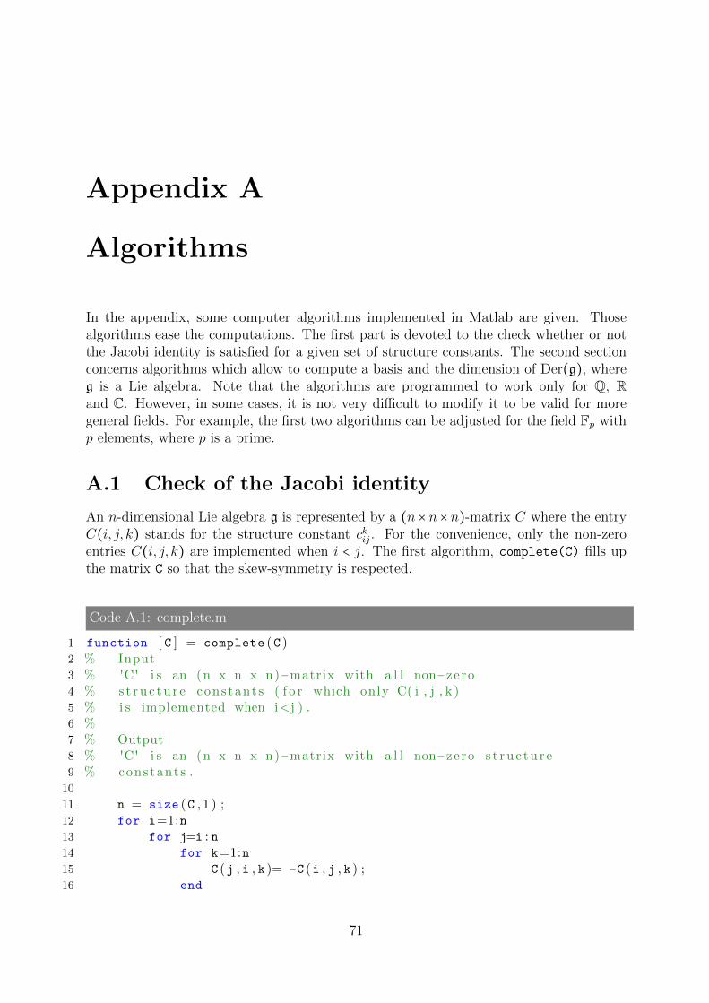
Appendix A
Algorithms
In the appendix, some computer algorithms implemented in Matlab are given. Thosealgorithms ease the computations. The first part is devoted to the check whether or notthe Jacobi identity is satisfied for a given set of structure constants. The second sectionconcerns algorithms which allow to compute a basis and the dimension of Der(g), whereg is a Lie algebra. Note that the algorithms are programmed to work only for Q, Rand C. However, in some cases, it is not very difficult to modify it to be valid for moregeneral fields. For example, the first two algorithms can be adjusted for the field Fp withp elements, where p is a prime.
A.1 Check of the Jacobi identity
An n-dimensional Lie algebra g is represented by a (n × n × n)-matrix C where the entryC(i, j, k) stands for the structure constant ckij. For the convenience, only the non-zeroentries C(i, j, k) are implemented when i < j. The first algorithm, complete(C) fills upthe matrix C so that the skew-symmetry is respected.
Code A.1: complete.m
1 function [ C ] = complete (C )2 % Input3 % 'C' i s an (n x n x n)−matrix with a l l non−zero4 % st ru c tu r e cons tant s ( f o r which only C( i , j , k )5 % i s implemented when i<j ) .6 %7 % Output8 % 'C' i s an (n x n x n)−matrix with a l l non−zero s t r u c tu r e9 % constant s .10
11 n = size (C , 1 ) ;12 for i=1:n13 for j=i : n14 for k=1:n15 C (j , i , k )= −C (i , j , k ) ;16 end
71
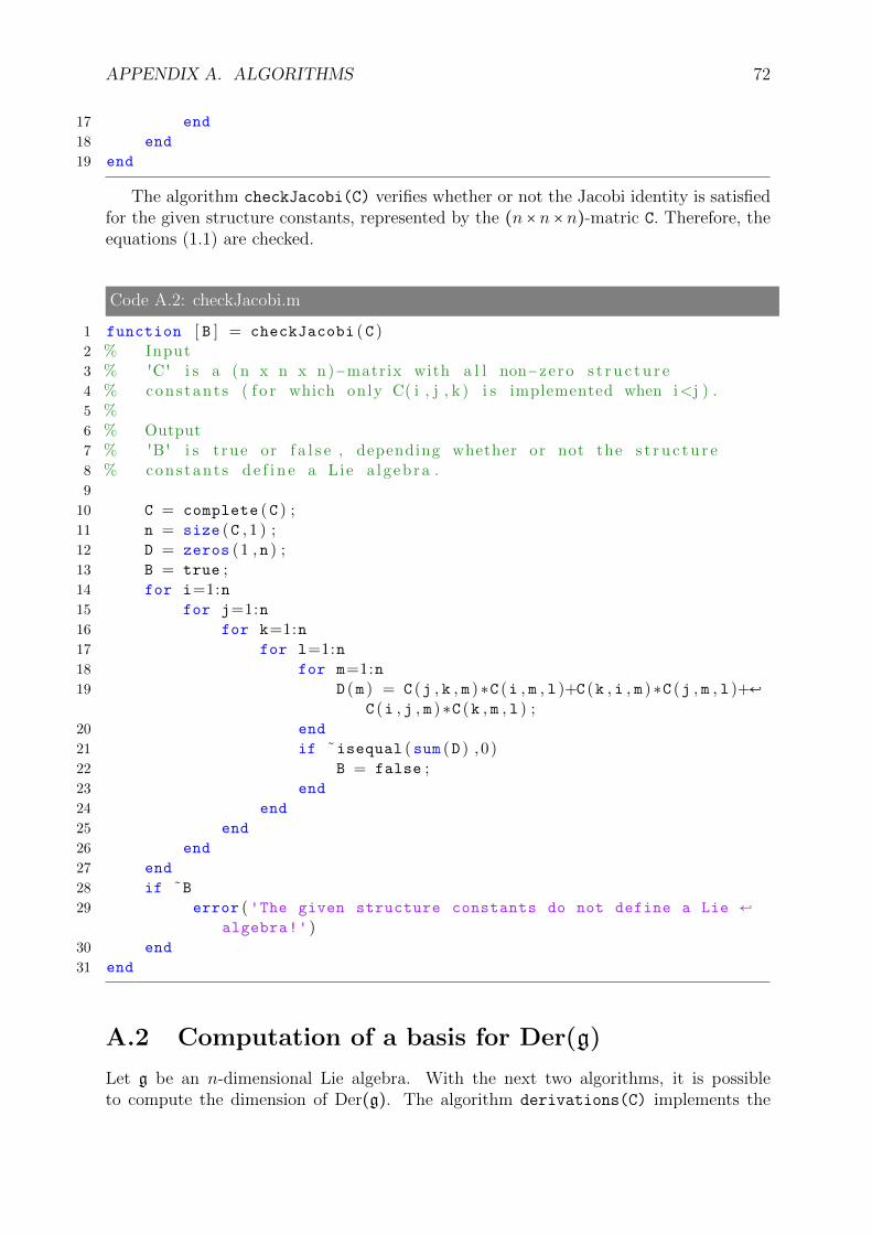
APPENDIX A. ALGORITHMS 72
17 end
18 end
19 end
The algorithm checkJacobi(C) verifies whether or not the Jacobi identity is satisfiedfor the given structure constants, represented by the (n × n × n)-matric C. Therefore, theequations (1.1) are checked.
Code A.2: checkJacobi.m
1 function [ B ] = checkJacobi (C )2 % Input3 % 'C' i s a (n x n x n)−matrix with a l l non−zero s t r u c tu r e4 % constant s ( f o r which only C( i , j , k ) i s implemented when i<j ) .5 %6 % Output7 % 'B ' i s t rue or f a l s e , depending whether or not the s t r u c tu r e8 % constant s d e f i n e a Lie a lgebra .9
10 C = complete (C ) ;11 n = size (C , 1 ) ;12 D = zeros (1 , n ) ;13 B = true ;14 for i=1:n15 for j=1:n16 for k=1:n17 for l=1:n18 for m=1:n19 D (m ) = C (j , k , m ) ∗C (i , m , l )+C (k , i , m ) ∗C (j , m , l )+↩
C (i , j , m ) ∗C (k , m , l ) ;20 end
21 if ˜isequal ( sum (D ) , 0 )22 B = false ;23 end
24 end
25 end
26 end
27 end
28 if ˜B29 error ('The given structure constants do not define a Lie ↩
algebra!' )30 end
31 end
A.2 Computation of a basis for Der(g)Let g be an n-dimensional Lie algebra. With the next two algorithms, it is possibleto compute the dimension of Der(g). The algorithm derivations(C) implements the
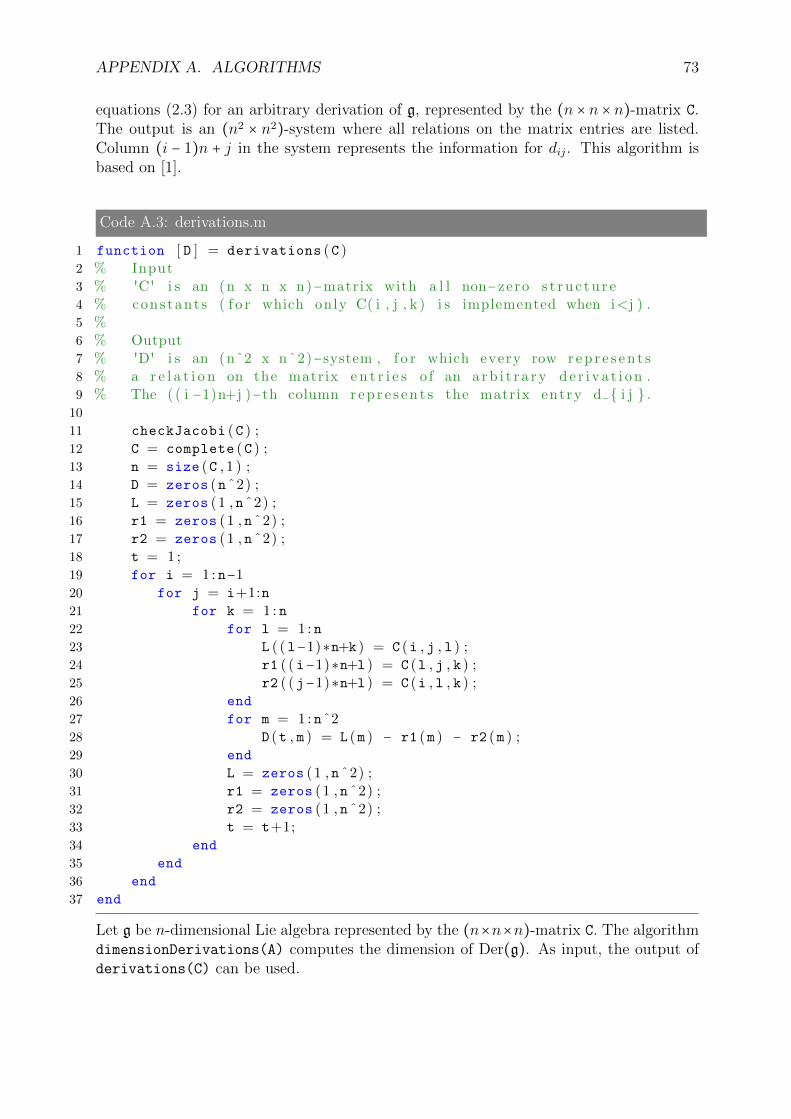
APPENDIX A. ALGORITHMS 73
equations (2.3) for an arbitrary derivation of g, represented by the (n × n × n)-matrix C.The output is an (n2 × n2)-system where all relations on the matrix entries are listed.Column (i − 1)n + j in the system represents the information for dij. This algorithm isbased on [1].
Code A.3: derivations.m
1 function [ D ] = derivations (C )2 % Input3 % 'C' i s an (n x n x n)−matrix with a l l non−zero s t r u c tu r e4 % constant s ( f o r which only C( i , j , k ) i s implemented when i<j ) .5 %6 % Output7 % 'D' i s an (nˆ2 x nˆ2)−system , f o r which every row r ep r e s en t s8 % a r e l a t i o n on the matrix e n t r i e s o f an a rb i t r a r y de r i v a t i on .9 % The ( ( i −1)n+j )−th column r ep r e s en t s the matrix entry d { i j } .10
11 checkJacobi (C ) ;12 C = complete (C ) ;13 n = size (C , 1 ) ;14 D = zeros (nˆ2) ;15 L = zeros (1 , nˆ2) ;16 r1 = zeros (1 , nˆ2) ;17 r2 = zeros (1 , nˆ2) ;18 t = 1 ;19 for i = 1 : n−120 for j = i+1:n21 for k = 1 : n22 for l = 1 : n23 L ( ( l−1)∗n+k ) = C (i , j , l ) ;24 r1 ( ( i−1)∗n+l ) = C (l , j , k ) ;25 r2 ( ( j−1)∗n+l ) = C (i , l , k ) ;26 end
27 for m = 1 : nˆ228 D (t , m ) = L (m ) − r1 (m ) − r2 (m ) ;29 end
30 L = zeros (1 , nˆ2) ;31 r1 = zeros (1 , nˆ2) ;32 r2 = zeros (1 , nˆ2) ;33 t = t+1;34 end
35 end
36 end
37 end
Let g be n-dimensional Lie algebra represented by the (n×n×n)-matrix C. The algorithmdimensionDerivations(A) computes the dimension of Der(g). As input, the output ofderivations(C) can be used.
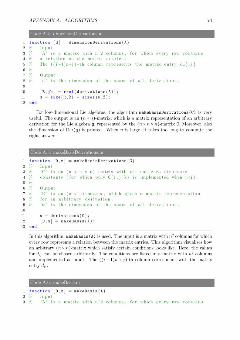
APPENDIX A. ALGORITHMS 74
Code A.4: dimensionDerivations.m
1 function [ d ] = dimensionDerivations (A )2 % Input3 % 'A' i s a matrix with nˆ2 columns , f o r which every row conta in s4 % a r e l a t i o n on the matrix e n t r i e s .5 % The ( ( i −1)n+j )−th column r ep r e s en t s the matrix entry d { i j } .6 %7 % Output8 % 'd ' i s the dimension o f the space o f a l l d e r i v a t i o n s .9
10 [ R , jb ] = rref ( derivations (A ) ) ;11 d = size (R , 2 ) − size (jb , 2 ) ;12 end
For low-dimensional Lie algebras, the algorithm makeBasisDerivations(C) is veryuseful. The output is an (n × n)-matrix, which is a matrix representation of an arbitraryderivation for the Lie algebra g, represented by the (n × n × n)-matrix C. Moreover, alsothe dimension of Der(g) is printed. When n is large, it takes too long to compute theright answer.
Code A.5: makeBasisDerivations.m
1 function [ D , m ] = makeBasisDerivations (C )2 % Input3 % 'C' i s an (n x n x n)−matrix with a l l non−zero s t r u c tu r e4 % constant s ( f o r which only C( i , j , k ) i s implemented when i<j ) .5 %6 % Output7 % 'D' i s an (n x n)−matrix , which g i v e s a matrix r ep r e s en t a t i on8 % fo r an a rb i t r a r y d e r i v a t i on .9 % 'm' i s the dimension o f the space o f a l l d e r i v a t i o n s .10
11 A = derivations (C ) ;12 [ D , m ] = makeBasis (A ) ;13 end
In this algorithm, makeBasis(A) is used. The input is a matrix with n2 columns for whichevery row represents a relation between the matrix entries. This algorithm visualises howan arbitrary (n × n)-matrix which satisfy certain conditions looks like. Here, the valuesfor dij can be chosen arbitrarily. The conditions are listed in a matrix with n2 columnsand implemented as input. The ((i − 1)n + j)-th column corresponds with the matrixentry dij.
Code A.6: makeBasis.m
1 function [ D , m ] = makeBasis (A )2 % Input3 % 'A' i s a matrix with nˆ2 columns , f o r which every row conta in s
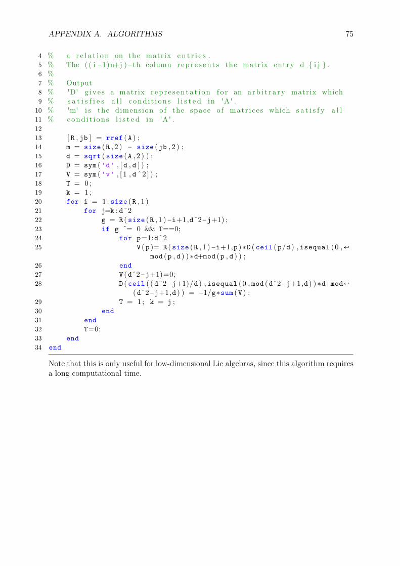
APPENDIX A. ALGORITHMS 75
4 % a r e l a t i o n on the matrix e n t r i e s .5 % The ( ( i −1)n+j )−th column r ep r e s en t s the matrix entry d { i j } .6 %7 % Output8 % 'D' g i v e s a matrix r ep r e s en t a t i on f o r an a rb i t r a r y matrix which9 % s a t i s f i e s a l l c ond i t i on s l i s t e d in 'A ' .10 % 'm' i s the dimension o f the space o f matr i ce s which s a t i s f y a l l11 % cond i t i on s l i s t e d in 'A ' .12
13 [ R , jb ] = rref (A ) ;14 m = size (R , 2 ) − size (jb , 2 ) ;15 d = sqrt ( size (A , 2 ) ) ;16 D = sym ('d' , [ d , d ] ) ;17 V = sym ('v' , [ 1 , d ˆ2 ] ) ;18 T = 0 ;19 k = 1 ;20 for i = 1 : size (R , 1 )21 for j=k : dˆ222 g = R ( size (R , 1 )−i+1,dˆ2−j+1) ;23 if g ˜= 0 && T==0;24 for p=1:dˆ225 V (p )= R ( size (R , 1 )−i+1,p ) ∗D ( ceil (p/d ) , isequal (0 ,↩
mod (p , d ) ) ∗d+mod (p , d ) ) ;26 end
27 V (dˆ2−j+1)=0;28 D ( ceil ( ( dˆ2−j+1)/d ) , isequal (0 , mod (dˆ2−j+1,d ) ) ∗d+mod↩
(dˆ2−j+1,d ) ) = −1/g∗sum (V ) ;29 T = 1 ; k = j ;30 end
31 end
32 T=0;33 end
34 end
Note that this is only useful for low-dimensional Lie algebras, since this algorithm requiresa long computational time.
Bibliography
[1] Vıctor Ayala, Eyup Kizil, and Ivan de Azevedo Tribuzy. On an algorithm for findingderivations of Lie algebras. Proyecciones, 31(1):81–90, 2012.
[2] Firmin Bratzlavsky. Classification des algebres de Lie nilpotentes de dimension n, declasse n − 1, dont l’ideal derive est commutatif. Acad. Roy. Belg. Bull. Cl. Sci. (5),60:858–865, 1974.
[3] Dietrich Burde. Lie Algebren und Darstellungstheorie. University Lecture (Univer-sitat Wien), 2006.
[4] Andreas Cap. Lie groups. University Lecture (Universitat Wien), 2015.
[5] Willem A. de Graaf. Lie algebras: theory and algorithms, volume 56 of North-HollandMathematical Library. North-Holland Publishing Co., Amsterdam, 2000.
[6] Dennis M. DeTurck and Carolyn S. Gordon. Isospectral deformations. I. Riemannianstructures on two-step nilspaces. Comm. Pure Appl. Math., 40(3):367–387, 1987.
[7] Dennis M. DeTurck and Carolyn S. Gordon. Isospectral deformations. II. Traceformulas, metrics, and potentials. Comm. Pure Appl. Math., 42(8):1067–1095, 1989.
[8] Karin Erdmann and Mark J. Wildon. Introduction to Lie algebras. Springer Under-graduate Mathematics Series. Springer-Verlag London, Ltd., London, 2006.
[9] Carolyn S. Gordon. The Laplace spectra versus the length spectra of Riemannianmanifolds. In Nonlinear problems in geometry (Mobile, Ala., 1985), volume 51 ofContemp. Math., pages 63–80. Amer. Math. Soc., Providence, RI, 1986.
[10] Carolyn S. Gordon and Ruth Gornet. Spectral geometry on nilmanifolds. In Progressin inverse spectral geometry, Trends Math., pages 23–49. Birkhauser, Basel, 1997.
[11] Carolyn S. Gordon and Yiping Mao. Comparisons of Laplace spectra, length spectraand geodesic flows of some Riemannian manifolds. Math. Res. Lett., 1(6):677–688,1994.
[12] Carolyn S. Gordon and Edward N. Wilson. Isospectral deformations of compactsolvmanifolds. J. Differential Geom., 19(1):241–256, 1984.
[13] Anatoly I. Malcev. On a class of homogeneous spaces. Amer. Math. Soc. Translation,1951(39):33, 1951.
76
BIBLIOGRAPHY 77
[14] John W. Milnor. Eigenvalues of the Laplace operator on certain manifolds. Proc.Nat. Acad. Sci. U.S.A., 51:542, 1964.
[15] Hubert Pesce. Deformations isospectrales sur certaines nilvarietes et finitude spec-trale des varietes de Heisenberg. Ann. Sci. Ecole Norm. Sup. (4), 25(5):515–538,1992.
[16] Ernst Witt. Treue Darstellung Liescher Ringe. J. Reine Angew. Math., 177:152–160,1937.

Algebraic Topology and Group TheoryEtienne Sabbelaan 53
8500 KORTRIJK, BELGIEtel. + 32 56 24 61 36