amsdottorato.unibo.itamsdottorato.unibo.it/4535/1/visani_davide_tesi.pdf · alma mater studiorum -...
TRANSCRIPT

Alma Mater Studiorum - Universita di Bologna
DOTTORATO DI RICERCA IN
INGEGNERIA ELETTRONICA, INFORMATICA E
DELLE TELECOMUNICAZIONI
Ciclo XXIV
Settore Concorsuale di afferenza: 09/F1 - Campi Elettromagnetici
Settore Scientifico disciplinare: ING-INF/02 - Campi Elettromagnetici
Fiber-Optic Technologies for Wirelineand Wireless In-building Networks
Presentata da: Relatore:
Ing. Davide Visani Prof. Ing. Giovanni Tartarini
Tutore:
Chiar.mo Prof. Ing. Paolo Bassi
Coordinatore Dottorato:
Chiar.mo Prof. Ing. Luca Benini
Esame finale anno 2012

Copyright c© 2012 by Davide Visani
All rights reserved. No part of this publication may be reproduced, stored
in a retrieval system, or transmitted in any form or by any means without
the prior written consent of the author.
Typeset using LATEX.

Abstract
This doctoral dissertation aims to establish fiber-optic technologies over-
coming the limiting issues of data communications in indoor environments.
Specific applications are broadband mobile distribution in different in-build-
ing scenarios and high-speed digital transmission over short-range wired op-
tical systems.
Two key enabling technologies are considered: Radio over Fiber (RoF)
techniques over standard silica fibers for distributed antenna systems (DASs)
and plastic optical fibers (POFs) for short-range communications.
The combination of RoF and DAS, which allows to shift the complex
electronic processing from the antenna base station towards a central office,
has already been recognized as a cost-effective solution for the radio cov-
erage of hostile propagation environments and scenarios with a high traffic
demand. However, the RoF technology is mainly limited to large locations,
such as stadiums, conference centers and university campi. The application
of RoF technologies to in-building scenarios needs to be deeply investigated in
conjunction with the exploitation of the available fiber infrastructures based
either on single or multi mode fibers.
POF is a well-known medium for short-range data communication with
two main advantages: the large-core size together with robustness and flexi-
bility, and the low cost mainly due to the use of silicon transceivers. Exten-
sive research activities on gigabit transmission over POF for home networking
have been performed in recent years. However, the ultimate exploitation of
i
ABSTRACT
POF for higher data rates and transport of wireless signals needs still to be
investigated.
The objectives of this thesis are related to the application of RoF and
POF technologies in different in-building scenarios.
On one hand, a theoretical and experimental analysis combined with
demonstration activities has been performed on cost-effective RoF systems
for the distribution of mobile signals over silica single and multi mode fibers.
On the other hand, digital signal processing techniques to overcome the
bandwidth limitation of POF have been investigated. In particular, dis-
crete multitone (DMT) modulation and novel constellation formats have been
studied with the purpose to maximize the transmission throughput of a POF
link. Moreover, the exploitation of POF for wireless signal distribution has
also been investigated.
The main achievements of the work included in this dissertation can be
summarized as follows:
• Theoretical and experimental characterization of distortion effects on a
radio multi-standard transmission over state-of-the-art intensity-modu-
lated direct-detection (IM–DD) RoF links over silica singlemode fiber
with directly modulated laser diodes (LDs). This activity was pursued
through modeling and measurements with third generation (3G) mobile
signals.
• Extensive modeling on modal noise impact both on linear and non-
linear characteristics of IM–DD RoF links over silica multimode fiber
with directly modulated LDs. The theoretical activity was validated
with experimental results leading to the definition of link design rules
for an optimum choice of the transmitter, receiver and launching tech-
nique.
• Successful transmission of Long Term Evolution (LTE) mobile signals
on the resulting optimized RoF system over silica multimode fiber em-
ploying a Fabry-Perot LD, central launch technique and a photodiode
ii

ABSTRACT
with a built-in ball lens. The performances were well compliant with
standard requirements up to 525 m of multimode fiber.
• Theoretical investigation and experimental demonstration of multi-
gigabit transmission over IM–DD POF links. An uncoded net bit-rate
of 5.15 Gbit/s was obtained on a 50 m long IM–DD POF link employ-
ing an eye-safe transmitter, a silicon photodiode, and DMT modulation
with bit and power loading algorithm.
• Insertion of 3 × 2N quadrature amplitude modulation (QAM) in the
constellations set of the DMT bit and power loading algorithm for
maximum capacity attainment in IM–DD POF links. An uncoded net
bit-rate of 5.4 Gbit/s was obtained on a 50 m long IM–DD POF link
employing an eye-safe transmitter and a silicon avalanche photodiode.
• Experimental validation of the simultaneous transmission of a multi-
gigabit baseband signal based on DMT and a radio frequency signal
based on ultra wideband (UWB) technology over a 50 m long IM–DD
POF link. An uncoded net bit-rate of 2 Gbit/s was obtained with
DMT, while a data stream of 200 Mbit/s was transported with the
UWB radio signal.
iii

ABSTRACT
iv

Contents
Abstract i
Contents v
Introduction 1
1 Technologies for in-building networks 5
1.1 Fiber technologies . . . . . . . . . . . . . . . . . . . . . . . . . 6
1.1.1 Silica optical fiber . . . . . . . . . . . . . . . . . . . . . 6
1.1.2 PMMA-based plastic optical fiber . . . . . . . . . . . . 10
1.2 Wireline communication technologies . . . . . . . . . . . . . . 13
1.2.1 Large and medium in-building networks . . . . . . . . 14
1.2.2 Home and small in-building networks . . . . . . . . . . 17
1.3 Wireless communication technologies . . . . . . . . . . . . . . 19
1.3.1 Large and medium in-building networks . . . . . . . . 24
1.3.2 Home and small in-building networks . . . . . . . . . . 26
1.4 Summary . . . . . . . . . . . . . . . . . . . . . . . . . . . . . 27
2 RoF systems over SMF for in-building F–DAS 29
2.1 Developed theoretical model . . . . . . . . . . . . . . . . . . . 29
2.1.1 Directly modulated laser . . . . . . . . . . . . . . . . . 30
2.1.1.1 Intensity modulation and TX non-linearities . 30
v
CONTENTS
2.1.1.2 Frequency chirping . . . . . . . . . . . . . . . 32
2.1.1.3 Electrical field . . . . . . . . . . . . . . . . . 34
2.1.2 Singlemode fiber propagation . . . . . . . . . . . . . . 36
2.1.3 Photodiode model . . . . . . . . . . . . . . . . . . . . 42
2.2 Experimental and theoretical results . . . . . . . . . . . . . . 44
2.2.1 Experimental setup . . . . . . . . . . . . . . . . . . . . 44
2.2.2 Experimental results and comparisons . . . . . . . . . 47
2.3 Summary . . . . . . . . . . . . . . . . . . . . . . . . . . . . . 52
3 RoF systems over MMF for in-building F–DAS 55
3.1 Developed theoretical model . . . . . . . . . . . . . . . . . . . 55
3.1.1 Electrical field produced by the laser . . . . . . . . . . 55
3.1.2 Multimode fiber launch and propagation . . . . . . . . 56
3.1.3 Receiver model . . . . . . . . . . . . . . . . . . . . . . 63
3.1.4 Extension to multi-wavelength sources . . . . . . . . . 75
3.2 Experimental and theoretical results . . . . . . . . . . . . . . 79
3.2.1 Experimental setup . . . . . . . . . . . . . . . . . . . . 79
3.2.2 Time behavior of received power . . . . . . . . . . . . . 81
3.2.3 Launch condition impact . . . . . . . . . . . . . . . . . 87
3.2.4 Receiver impact . . . . . . . . . . . . . . . . . . . . . . 92
3.2.5 Transmitter impact . . . . . . . . . . . . . . . . . . . . 96
3.2.5.1 Comparison of transmitters based on DFB laser 96
3.2.5.2 Comparison of trasmitters based on FP laser 104
3.3 LTE transmission experiments . . . . . . . . . . . . . . . . . . 110
3.4 Summary . . . . . . . . . . . . . . . . . . . . . . . . . . . . . 116
4 POF systems for home area networks 119
4.1 Model for the channel capacity of IM–DD POF links . . . . . 119
4.2 High capacity transmission over GI–POF employing DMT . . 130
4.2.1 Bit and power loading in DMT . . . . . . . . . . . . . 130
4.2.2 Experimental setup . . . . . . . . . . . . . . . . . . . . 133
4.2.3 50 m PMMA GI–POF transmission with APD . . . . . 140
4.2.4 50 m PMMA GI–POF transmission with PIN PD . . . 144
vi

CONTENTS
4.2.5 Evaluation of DMT and optical link parameters . . . . 147
4.3 3× 2N–QAM constellations for DMT . . . . . . . . . . . . . . 151
4.3.1 Application to 50 m PMMA GI–POF link with APD . 154
4.4 Summary . . . . . . . . . . . . . . . . . . . . . . . . . . . . . 158
5 POF systems for converged home area networks 161
5.1 Ultra wideband technologies . . . . . . . . . . . . . . . . . . . 161
5.2 Converged transmission of baseband DMT and UWB signals . 163
5.2.1 Experimental setup . . . . . . . . . . . . . . . . . . . . 163
5.2.2 Experimental results and discussion . . . . . . . . . . . 165
5.3 Summary . . . . . . . . . . . . . . . . . . . . . . . . . . . . . 173
Conclusions 175
Bibliography 181
List of acronyms 195
List of publications 201
Acknowledgments 207
vii

CONTENTS
viii

Introduction
“Broadband access for everyone, everywhere”. This is one popular motto
of the information and communications technology (ICT) community since
the rising of broadband wireline and wireless technologies. The possibility to
use broadband services wherever you are (everywhere) and at an affordable
price (everyone) was an added benefit provided by wireless broadband tech-
nologies since the first introduction of the third generation (3G) mobile net-
work. For this reason, telecom operators have put considerable efforts in the
last decade on wireline last-mile solutions and wireless coverage. Although
wireline and wireless access technologies are considered as competitors, they
have one thing in common: they are mostly deployed outdoor. However, the
majority of the broadband traffic is generated inside premises by devices us-
ing wireless connections, such as smartphones and tablets, or using wireline
connections, such as desktop PCs and data centers. Until now, the indus-
try did not put a large emphasis on planning for in-building deployments
capable of supporting new broadband telecommunication services, such as
new video-based services and advanced Internet applications. But, this is
expected to become soon a basic necessity.
The chances that telecom operators will solve every in-building wireline
and wireless coverage issue are very slim. Hence, technical solutions are
highly case-dependent and mainly based on a compromise between present
service requirements, future-proofness and cost. In this framework, fiber-
optic technologies are typically considered an answer to the request to be
1
INTRODUCTION
Wireline
Wireless
SMF
100 G local area networks,… 3G/4G mobile signals transport up to several kilometers
(Chapter 2)
MMF
10 G local area networks,… 3G/4G mobile signals transport up to 500 m
(Chapter 3)
POF
MulE-‐gigabit serial data transmission
(Chapter 4)
Transport of UWB radio signal and mulE-‐gigabit data transmission
(Chapter 5)
Fiber
Service Large and m
edium buildings S
mall buildings
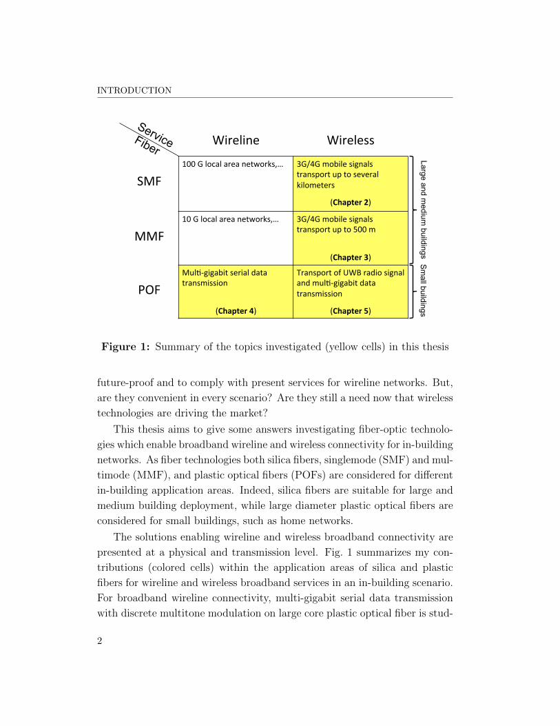
Figure 1: Summary of the topics investigated (yellow cells) in this thesis
future-proof and to comply with present services for wireline networks. But,
are they convenient in every scenario? Are they still a need now that wireless
technologies are driving the market?
This thesis aims to give some answers investigating fiber-optic technolo-
gies which enable broadband wireline and wireless connectivity for in-building
networks. As fiber technologies both silica fibers, singlemode (SMF) and mul-
timode (MMF), and plastic optical fibers (POFs) are considered for different
in-building application areas. Indeed, silica fibers are suitable for large and
medium building deployment, while large diameter plastic optical fibers are
considered for small buildings, such as home networks.
The solutions enabling wireline and wireless broadband connectivity are
presented at a physical and transmission level. Fig. 1 summarizes my con-
tributions (colored cells) within the application areas of silica and plastic
fibers for wireline and wireless broadband services in an in-building scenario.
For broadband wireline connectivity, multi-gigabit serial data transmission
with discrete multitone modulation on large core plastic optical fiber is stud-
2
INTRODUCTION
ied for small building deployment. For in-building wireless connectivity, two
main categories are investigated. For large and medium building deployment,
radio over fiber techniques for fiber distributed antenna systems employing
silica fibers are studied as an enabling technology for the efficient distribu-
tion of 3G and fourth generation (4G) mobile services. For small buildings,
the feasibility of a converged optical infrastructure based on plastic optical
fiber supporting wireless signal transport and multi-gigabit baseband data
transmission is inquired.
The thesis is organized in five chapters.
Chapter 1 gives an overview of the optical properties of silica fibers and
large diameter plastic optical fibers. Hence, the application of these fiber
media to the distribution of wireline and wireless communication technologies
is depicted and referred to the in-building application scenario.
Chapter 2 presents a numerical model for the evaluation of the trans-
mission performance of real radio signals in radio over fiber links employing
directly modulated lasers and singlemode fiber. Transmission experiments
are also shown and compared with the simulated results.
Chapter 3 reports the modeling and experimental activity on radio over
fiber links employing directly modulated lasers and multimode fiber. The
developed model describes the impact of modal noise on linear and non-linear
characteristics of the link. The experimental results are used to confirm the
model prediction and to design a radio over multimode fiber link with good
characteristics. Finally, transmission experiments are shown.
Chapter 4 presents the research activity on multi-gigabit transmission
over large diameter plastic optical fibers. A model for the estimation of the
channel capacity is derived. Multi-gigabit transmission experiments employ-
ing discrete multitone modulation with bit-loading are presented. Finally,
constellation formats transporting a fractional number of bits per symbol
are introduced and applied to transmission experiments with discrete multi-
tone modulation and bit-loading.
Chapter 5 reports the experimental activity on the simultaneous trans-
mission of an ultra wideband radio signal and a multi-gigabit data stream
based on discrete multitone modulation.
3

INTRODUCTION
Finally, the achieved results are summarized with a unified approach in
the Conclusions section.
The work presented in this thesis is the outcome of my Ph.D. research
activity at the “Dipartimento di Elettronica, Informatica e Sistemistica”
(DEIS) of the University of Bologna within the European FP7 project 212352
ICT “Architectures for fLexible Photonic Home and Access networks”
(ALPHA). Part of this work was performed in collaboration with Comm-
scope Italy S.r.l. Part of this work is a result of a research period at the
COBRA Research Institute of the Eindhoven University of Technology, The
Netherlands.
4
Chapter 1Technologies for in-building networks
In this chapter an overview of fiber-optic technologies and solutions for
in-building networks are presented. An in-building network can be defined as
a communication system which connects devices and users inside a premise
with each other and with the external networks, i.e. access and/or mobile
networks.
In section 1.1 classification and main properties of optical fibers based on
silica and Poly(methyl methacrylate) (PMMA) will be illustrated.
In section 1.2 and 1.3 the appropriate fiber-optic technology for large/me-
dium buildings and small buildings is discussed. Section 1.2 refers to the
distribution of wireline services, in particular referred to high-speed local
area and home networks. Section 1.3 describes the distribution of wireless
services, with emphasis on in-building radio coverage with current and emerg-
ing wireless standards. In this dissertation, I considered separately wireline
and wireless services since the proposed solutions needs to meet different
service requirements.
5
CHAPTER 1. TECHNOLOGIES FOR IN-BUILDING NETWORKS
125 µm
62.5 µm 50 µm ≈ 9 µm
SMF 50/125 MMF
62.5/125 MMF
Operating wavelenghts
1310-1625 nm 850 nm and 1310 nm
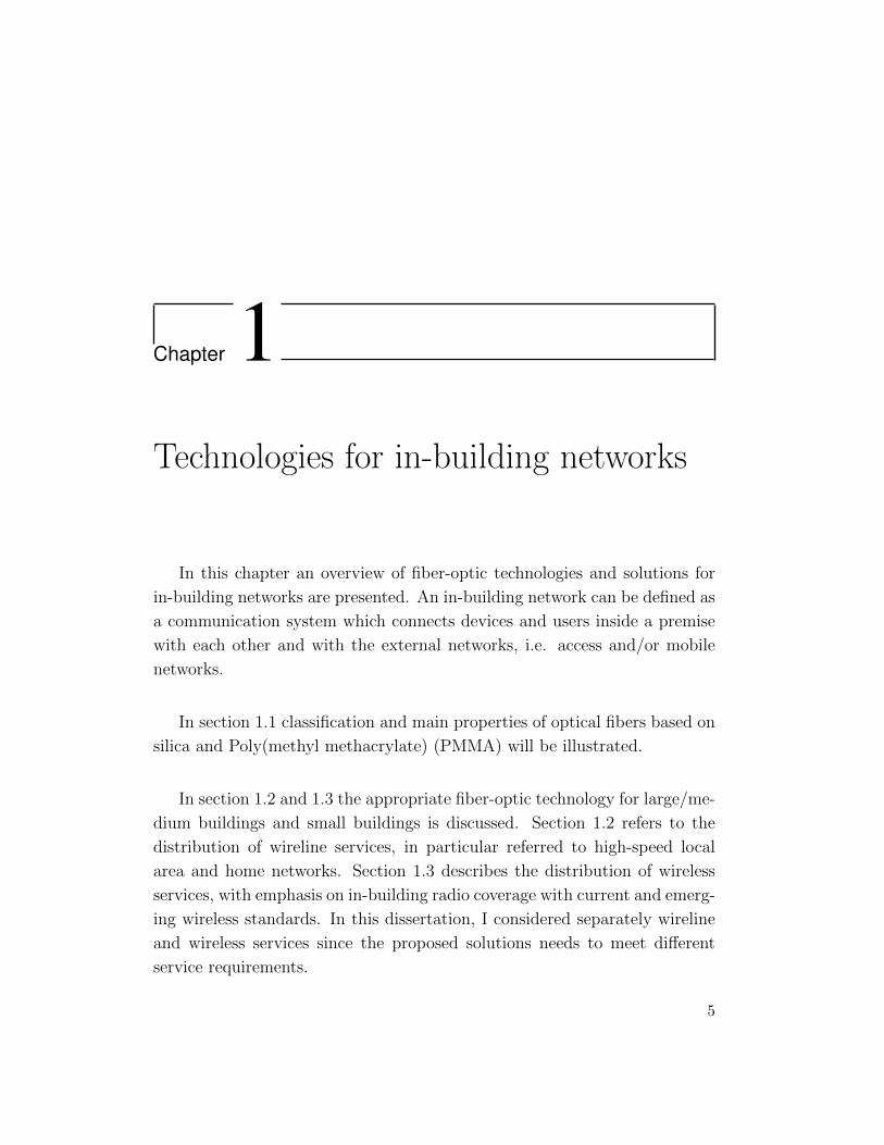
Figure 1.1: Schematic drawing of multimode and singlemode fibers
1.1 Fiber technologies
1.1.1 Silica optical fiber
Silica optical fiber is by definition the optical fiber for data communica-
tion. It consists of two silica-based materials: a higher refractive index core
and a lower refractive index cladding. As summarized in Fig. 1.1 there are
two main types of silica optical fiber: multimode and singlemode fiber. Mul-
timode fiber (MMF) for data communications has a core diameter of 62.5
or 50 µm, a cladding diameter of 125 µm, and is used in the 850 nm and
1310 nm spectral windows. Singlemode fiber (SMF) has a narrow core di-
ameter of about 9 µm, a cladding diameter of 125 µm, and is used between
1310 and 1625 nm. I will not consider in this work other silica-based optical
fibers such as plastic and hard polymer clad silica fibers, where a silica core is
surrounded by a thin plastic polymer material [1], or photonic crystal fibers,
in which the light is guided by a reduced effective index of the cladding or
by a photonic bandgap effect [2].
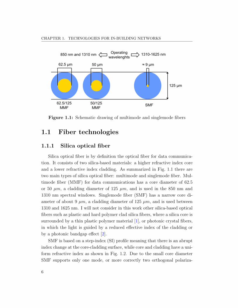
SMF is based on a step-index (SI) profile meaning that there is an abrupt
index change at the core-cladding surface, while core and cladding have a uni-
form refractive index as shown in Fig. 1.2. Due to the small core diameter
SMF supports only one mode, or more correctly two orthogonal polariza-
6
1.1. FIBER TECHNOLOGIES
Step-index (SI) Graded-index (GI)
Refractive index profile
Figure 1.2: Schematic drawing of step-index and graded-index profiles
tion modes whose different propagation properties are revealed after long
transmission distances [3]. SMF is standardized under several international
standards. One of the most known is the ITU–T G.652 recommendation of
the International Telecommunication Union (ITU) [4]. The typical optical
attenuation is 0.2 dB/km at 1550 nm and 0.35 dB/km at 1310 nm which,
together with the availability of optical amplifiers, allows for long-haul trans-
mission [5]. The bandwidth (BW) per distance product of SMF systems is
typically limited by the modulating signal bandwidth of the transmitter (TX)
and the receiver (RX) in short-range transmission and by the effects of chro-
matic dispersion, polarization mode dispersion and non-linearity in medium
and long-haul transmission [3].
MMF for data communication is designed with a graded-index (GI) profile
where the refractive index decreases gradually from the center of the core to
the cladding as shown in Fig. 1.2. Since MMF core diameter is more than
five times larger than SMF core diameter, MMF supports a large number
of guided modes. This characteristic produces a strong BW limitation of
MMF compared to SMF. Indeed, because of an effect similar to multi-path
propagation in a radio channel, the BW of MMF systems is typically limited
by modal dispersion. Chromatic dispersion, polarization mode dispersion and
7
CHAPTER 1. TECHNOLOGIES FOR IN-BUILDING NETWORKS
non-linear effects are also present in MMF systems, but their contributions
are typically negligible with respect to modal dispersion. To minimize modal
dispersion an accurate design of the GI profile is employed. However, modal
dispersion compensation depends in an critical manner on the refractive index
profile and so modal dispersion can be minimized just for a small interval of
operating wavelengths [6].
θmax
NA = 0.275 for 62.5/125 MMF NA = 0.200 for 50/125 MMF
NA = sin(θmax) (coming from air)
(a) Multimode fiber
NA = sin(θmax) (coming from air)
NA ≈ 0.1 for SMF
θmax
(b) Singlemode fiber
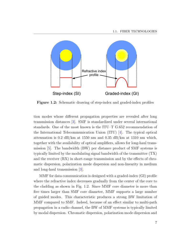
Figure 1.3: Schematic drawing of numerical aperture of multimode (a) and
singlemode (b) fibers
MMF is standardized under ISO/IEC 11801 standards and ITU–T G.651.1
(only 50/125 MMF) [7, 8], but also the TIA–492AAAx classification is often
used [9]. The maximum optical attenuation should comply with the values
of 3.5 dB/km at 850 nm and 1 dB/km at 1310 nm, while the numerical
aperture (NA) is set to 0.2 for 50/125 MMF and 0.275 for 62.5/125 MMF.
Fig. 1.3 shows graphically the meaning of the numerical aperture which is
related to the half-angle θmax of the maximum cone of light that can enter or
8
1.1. FIBER TECHNOLOGIES
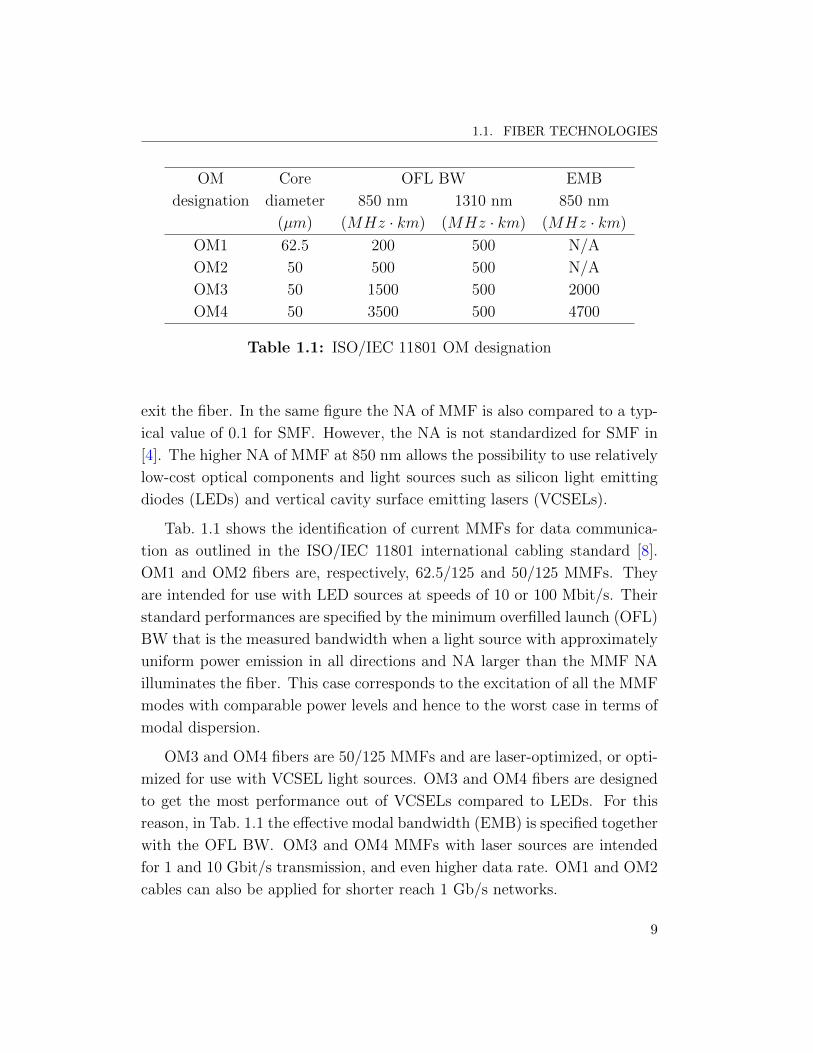
OM Core OFL BW EMB
designation diameter 850 nm 1310 nm 850 nm
(µm) (MHz · km) (MHz · km) (MHz · km)
OM1 62.5 200 500 N/A
OM2 50 500 500 N/A
OM3 50 1500 500 2000
OM4 50 3500 500 4700
Table 1.1: ISO/IEC 11801 OM designation
exit the fiber. In the same figure the NA of MMF is also compared to a typ-
ical value of 0.1 for SMF. However, the NA is not standardized for SMF in
[4]. The higher NA of MMF at 850 nm allows the possibility to use relatively
low-cost optical components and light sources such as silicon light emitting
diodes (LEDs) and vertical cavity surface emitting lasers (VCSELs).
Tab. 1.1 shows the identification of current MMFs for data communica-
tion as outlined in the ISO/IEC 11801 international cabling standard [8].
OM1 and OM2 fibers are, respectively, 62.5/125 and 50/125 MMFs. They
are intended for use with LED sources at speeds of 10 or 100 Mbit/s. Their
standard performances are specified by the minimum overfilled launch (OFL)
BW that is the measured bandwidth when a light source with approximately
uniform power emission in all directions and NA larger than the MMF NA
illuminates the fiber. This case corresponds to the excitation of all the MMF
modes with comparable power levels and hence to the worst case in terms of
modal dispersion.
OM3 and OM4 fibers are 50/125 MMFs and are laser-optimized, or opti-
mized for use with VCSEL light sources. OM3 and OM4 fibers are designed
to get the most performance out of VCSELs compared to LEDs. For this
reason, in Tab. 1.1 the effective modal bandwidth (EMB) is specified together
with the OFL BW. OM3 and OM4 MMFs with laser sources are intended
for 1 and 10 Gbit/s transmission, and even higher data rate. OM1 and OM2
cables can also be applied for shorter reach 1 Gb/s networks.
9

CHAPTER 1. TECHNOLOGIES FOR IN-BUILDING NETWORKS
1.1.2 PMMA-based plastic optical fiber
MMF 50/125 µm
SMF 9/125 µm
PMMA POF 980/1000 µm
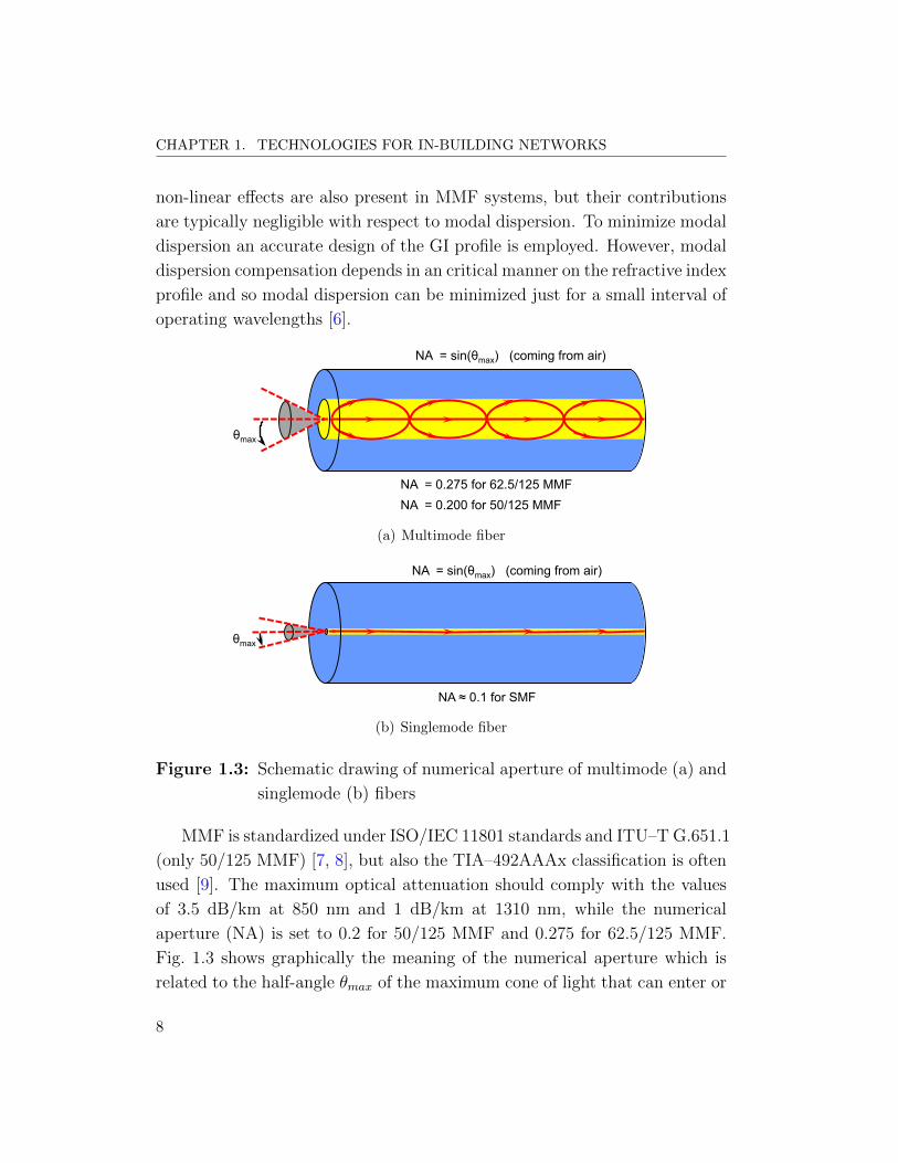
Figure 1.4: Comparison of the fiber core diameters for (left-to-right) SMF,
50/125 MMF and 1 mm diameter PMMA SI–POF
An optical fiber based on silica is also called a glass optical fiber (GOF).
Due to the intrinsic nature of glass materials the size of the core of GOF
cannot overcome approximately 200 µm without incurring in mechanical
stiffness. However, other materials can be employed to manufacture opti-
cal fibers. Utilizing polymer, or plastic, materials it is possible to obtain
plastic optical fibers (POFs). POFs can have a large core diameter of 0.5
and 1 mm keeping flexibility and mechanical resistance [10]. This leads to a
simpler termination, splicing, connectorization, and coupling between a light
source and the fiber compared to GOF.
Among polymer materials, Poly(methyl methacrylate) (PMMA) is the
most popular and used material for POFs. Fig. 1.4 shows a comparison
between the cross section of SMF, 50/125 MMF and 1 mm diameter PMMA
SI–POF. As suggested in the figure, a PMMA based SI–POF has a core
10
1.1. FIBER TECHNOLOGIES
1
0.01
0.1
450 500 550 600 650 700 400
Loss
(dB
/m)
step-index
graded-index
multi-core
Loss
(dB
/km
)
100
10
1000
Wavelength (nm)
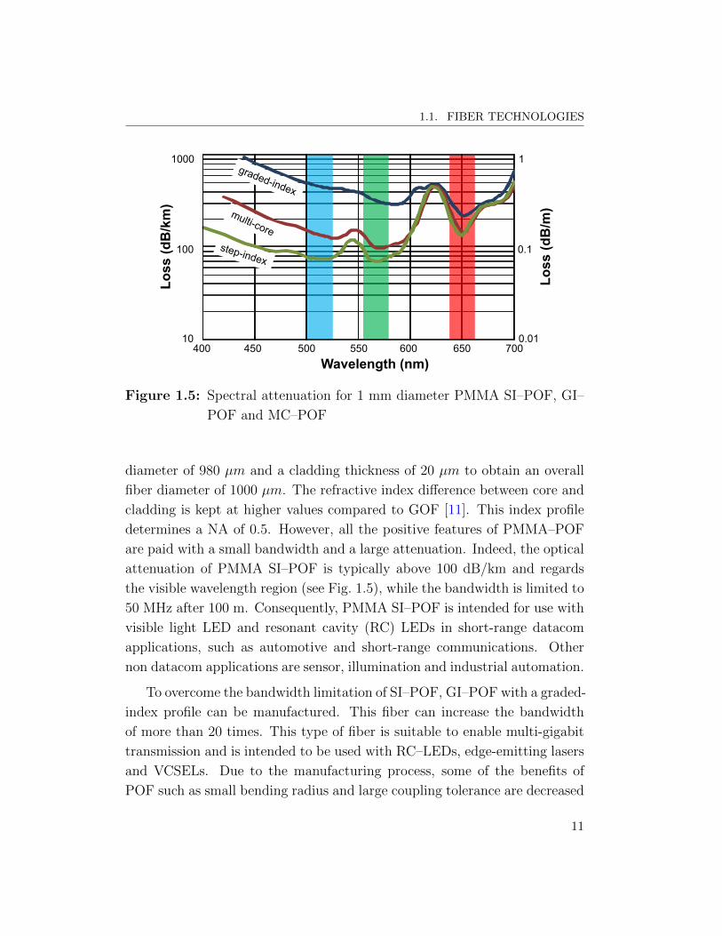
Figure 1.5: Spectral attenuation for 1 mm diameter PMMA SI–POF, GI–
POF and MC–POF
diameter of 980 µm and a cladding thickness of 20 µm to obtain an overall
fiber diameter of 1000 µm. The refractive index difference between core and
cladding is kept at higher values compared to GOF [11]. This index profile
determines a NA of 0.5. However, all the positive features of PMMA–POF
are paid with a small bandwidth and a large attenuation. Indeed, the optical
attenuation of PMMA SI–POF is typically above 100 dB/km and regards
the visible wavelength region (see Fig. 1.5), while the bandwidth is limited to
50 MHz after 100 m. Consequently, PMMA SI–POF is intended for use with
visible light LED and resonant cavity (RC) LEDs in short-range datacom
applications, such as automotive and short-range communications. Other
non datacom applications are sensor, illumination and industrial automation.
To overcome the bandwidth limitation of SI–POF, GI–POF with a graded-
index profile can be manufactured. This fiber can increase the bandwidth
of more than 20 times. This type of fiber is suitable to enable multi-gigabit
transmission and is intended to be used with RC–LEDs, edge-emitting lasers
and VCSELs. Due to the manufacturing process, some of the benefits of
POF such as small bending radius and large coupling tolerance are decreased
11
CHAPTER 1. TECHNOLOGIES FOR IN-BUILDING NETWORKS
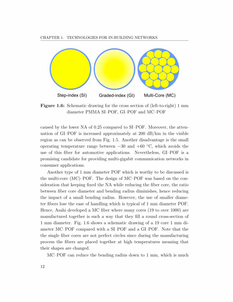
Step-index (SI) Graded-index (GI) Multi-Core (MC)
Figure 1.6: Schematic drawing for the cross section of (left-to-right) 1 mm
diameter PMMA SI–POF, GI–POF and MC–POF
caused by the lower NA of 0.25 compared to SI–POF. Moreover, the atten-
uation of GI–POF is increased approximately at 200 dB/km in the visible
region as can be observed from Fig. 1.5. Another disadvantage is the small
operating temperature range between −30 and +60 C, which avoids the
use of this fiber for automotive applications. Nevertheless, GI–POF is a
promising candidate for providing multi-gigabit communication networks in
consumer applications.
Another type of 1 mm diameter POF which is worthy to be discussed is
the multi-core (MC)–POF. The design of MC–POF was based on the con-
sideration that keeping fixed the NA while reducing the fiber core, the ratio
between fiber core diameter and bending radius diminishes, hence reducing
the impact of a small bending radius. However, the use of smaller diame-
ter fibers lose the ease of handling which is typical of 1 mm diameter POF.
Hence, Asahi developed a MC fiber where many cores (19 to over 1000) are
manufactured together is such a way that they fill a round cross-section of
1 mm diameter. Fig. 1.6 shows a schematic drawing of a 19 core 1 mm di-
ameter MC–POF compared with a SI–POF and a GI–POF. Note that the
the single fiber cores are not perfect circles since during the manufacturing
process the fibers are placed together at high temperatures meaning that
their shapes are changed.
MC–POF can reduce the bending radius down to 1 mm, which is much
12

1.2. WIRELINE COMMUNICATION TECHNOLOGIES
Fiber type Loss at 650 nm BW-length product NA Bending radius
(dB/km) (MHz · km) (mm)
SI–POF < 160 5 0.5 20
GI–POF < 200 > 100 0.25 25
MC–POF < 160 > 20 0.6 1-3
Table 1.2: Characteristics of some 1 mm diameter PMMA POF
less than 20 mm for SI–POF and 25 mm for GI–POF. The optical attenuation
of MC–POF is similar to the one of SI–POF as shown in Fig. 1.5. Due to a
NA of 0.6 and to the step-index profile of each fiber core MC–POF should
have bandwidth properties similar to SI–POF. However, the measured values
are actually higher than the one of SI–POF. This fact has been explained
by means of mode coupling and mode-selective attenuation [11].
Tab. 1.2 summarizes the main optical properties of SI–POF, GI–POF
and MC–POF. I underline that 1 mm diameter SI–POF is at present the
only standardized cable for indoor applications under A4a category in IEC
60793-2-40 standard [12]. GI–POF and MC–POF are not yet standardized,
hence limiting their widespread availability and causing higher prices due the
lack of a volume market.
1.2 Wireline communication technologies
At present, most of the services offered to an in-building device or user
are completely or partially transported by a wired network. Some example
of current services are VoIP, IPTV, Internet related applications, like large
file-sharing, high-definition video streaming. The current wired technologies
are mostly based on copper cables, such as twisted-pair, Category 5 (Cat-5),
coaxial, and power-lines. With Cat-5 technology a throughput of 100 Mbit/s
(officially 100 BASE-TX, known as Fast-Ethernet) is possible up to 100 m
under any operating condition [13]. Also Gigabit Ethernet (1000BASE-T)
is possible on Cat-5 up to 100 m [14], but under controlled operating condi-
tion, e.g. limited bending condition and electromagnetic interference. Higher
13

CHAPTER 1. TECHNOLOGIES FOR IN-BUILDING NETWORKS
Vertical distribution: • MMF or SMF
Horizontal distribution: • Predominately copper
(10/100/1000 Ethernet) • POF as alternative • Silica fiber for higher speed
Access network
Figure 1.7: Large and medium buildings wireline network
speeds are instead not feasible with Cat-5 and requires higher-quality cables
(Category 6 or better) [15]. In the framework of this limitation for copper
wires, fiber-optic cables show their advantages. Indeed, SMF is a future-
proof transmission medium, whose bandwidth per length product can be
considered unlimited for in-building application, and limited just by the cur-
rent transceiver technology. Anyway, SMF–based in-building networks have
a cost which is not suitable for every scenario. For this reason, I divide the
deployment choice among fiber-optic cables on the network size, i.e. usually
the building size.
1.2.1 Large and medium in-building networks
For large and medium building networks I consider a telecommunication
network deployed over several floors and rooms. Some examples of a large
building are a shopping mall, a large corporate building, and a sport-center,
14
1.2. WIRELINE COMMUNICATION TECHNOLOGIES
while medium buildings are a medium corporate building, a full-service hotel,
and a school. The wired coverage of these scenarios with fiber-optic solutions
is currently implemented as shown in Fig. 1.7.
The vertical distribution from the bottom to the top of the building is
performed with silica SMF or MMF due to the large amount of data which
needs to be delivered. For horizontal, or floor, distribution copper technolo-
gies are currently employed, mostly Cat-5 and Cat-6. This is due to the
lower amount of data to be distributed, typically 100/1000 Mbit/s, and to
the short requested range, typically around 100 m. As an optical alternative
to copper solutions, standard POF can be employed as it will be described in
section 1.2.2. For future-proof deployment or when the requested data rate
or range increases, silica fiber gains attraction.
Although SMF has a fundamental larger bandwidth compared to MMF,
there is still an increasing interest to install silica MMF in an indoor scenario.
This is not due to a lower fiber cost per unit length, since from this point
of view there is no advantage to choose MMF. However, there are other
aspects, rather than fiber cost, which are more favorable for MMF than for
SMF:
• SMF has a much smaller core diameter, and hence needs very accu-
rate tools for splicing and connectorizing, plus highly-skilled installers.
Thus, splicing and connectorizing of MMF is cheaper
• Due to its small core diameter, a SMF connection is more vulnerable
for contamination by dust and scratches, as may happen easily in de-
tachable connections in in-building networks. The larger core size of
MMF significantly relaxes these contamination problems
• For wavelengths below 1 µm, silicon photodetectors may be used, which
offer the advantage of co-integration with the electronic circuitry in a
single silicon-based receiver integrated circuit. This enables really low-
cost receiver modules and reduced power consumption. However, a
standard SMF is no longer single-mode at wavelengths below its cut-
off wavelength, typically around 1.2 µm. On the other hand, silica
15
CHAPTER 1. TECHNOLOGIES FOR IN-BUILDING NETWORKS
SMF MMF
Information carrying capacity ×Distance supported ×
Fiber price ×Transceiver and connector price ×
Ease of handling ×Transceiver power consumption ×
Table 1.3: Comparison of the advantages of SMF and MMF for in-building
networks
MMF operates fine at wavelengths in the 850 nm near infra-red region
In addition to this green-field installation advantages, silica MMF is al-
ready installed in many premises and thus it can be used as a basis for
a network upgrade. Related to the previous list, Tab. 1.3 summarizes the
main advantages of using SMF or MMF solutions.
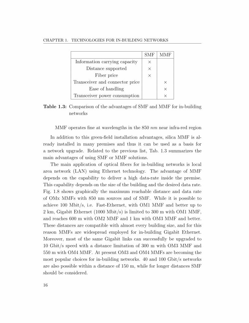
The main application of optical fibers for in-building networks is local
area network (LAN) using Ethernet technology. The advantage of MMF
depends on the capability to deliver a high data-rate inside the premise.
This capability depends on the size of the building and the desired data rate.
Fig. 1.8 shows graphically the maximum reachable distance and data rate
of OMx MMFs with 850 nm sources and of SMF. While it is possible to
achieve 100 Mbit/s, i.e. Fast-Ethernet, with OM1 MMF and better up to
2 km, Gigabit Ethernet (1000 Mbit/s) is limited to 300 m with OM1 MMF,
and reaches 600 m with OM2 MMF and 1 km with OM3 MMF and better.
These distances are compatible with almost every building size, and for this
reason MMFs are widespread employed for in-building Gigabit Ethernet.
Moreover, most of the same Gigabit links can successfully be upgraded to
10 Gbit/s speed with a distance limitation of 300 m with OM3 MMF and
550 m with OM4 MMF. At present OM3 and OM4 MMFs are becoming the
most popular choices for in-building networks. 40 and 100 Gbit/s networks
are also possible within a distance of 150 m, while for longer distances SMF
should be considered.
16
1.2. WIRELINE COMMUNICATION TECHNOLOGIES
100000
40000
10000
1000
100
10
82 100 150 300 550
600
1000 2000
OM3
OM3
OM3 OM4
OM4
SMF
Distance (m)
Dat
a ra
te (M
bit/s
)
33
OM2
OM2
OM1
Figure 1.8: Fiber choices depending on requested data rate and distance
with OMx MMF using 850 nm sources and with SMF
These technical considerations conclude that MMF can be considered a
future-proof solution for medium building networks. For data rate above
100 Gbit/s and for large buildings networks SMF should be instead consid-
ered.
1.2.2 Home and small in-building networks
For small building networks I refer to a telecommunication network de-
ployed over the premise of a small enterprise or a family house with maximum
three floors and three rooms per floor.
Small in-building networks are more cost-sensitive than large and medium
in-building networks because fewer users are sharing equipment and installa-
tion costs. Particularly, in home area networks (HANs) there is no sharing of
costs at all. Furthermore, the installation costs typically exceed the equip-
ment costs per user. Therefore, the focus on home and small in-building
networks should be on keeping installation costs at a minimum level. While
17

CHAPTER 1. TECHNOLOGIES FOR IN-BUILDING NETWORKS
for some small building networks silica MMF can be still considered as a
good tradeoff between performance and cost, a fiber-optic solution with a
potential lower cost need to be considered for home networks.
On this basis, POF is an interesting solution to be applied in low-cost
short-range optical communication systems. Indeed, 1 mm diameter POF
has interesting characteristics for small networks compared to silica fibers:
• Easy coupling with sources and no strict needs for connectors
• Use of cheap visible light sources such as LED
• Robustness against mechanical stress and bending
All these positive features of POF have as counterpart its limited band-
width compared to silica fibers. However, the real competitors of POF in
small in-building networks are copper technologies, e.g. Cat-5. POF so-
lutions are already commercially available for Fast-Ethernet (100 Mbit/s)
within a distance of 100 m. This is the same data-rate and distance target of
Cat-5 solutions. With respect to Cat-5, POF cable has diameter of 2.2 mm
which offers multiple ways to be installed. Moreover, it can be installed
separately or in combination with other cables such as power-line, twisted-
pair and coaxial cabling due to electromagnetic immunity (EMI). The easy
of handling and the use of visible light makes POF an attractive candidate
for do-it-yourself installation, meaning that there is no mandatory need for
professional installation.
Research studies have demonstrated the possibility to increase the perfor-
mance of standard SI–POF to 1 Gbit/s up to 75 m [16, 17]. Higher data-rates
have been demonstrated utilizing GI–POF or MC–POF [18].
The possibility to have a gigabit or more optical backbone in a small
building scenario is crucial to distribute all the residential or office services
in a single infrastructure. Currently, a plethora of delivery methods and ca-
ble media are employed for different kinds of wireline services; e.g., coaxial
cabling for video broadcast, Cat-5 cabling for LAN, twisted pair cable for
wired telephony and internet access. Such multiple network infrastructure
18
1.3. WIRELESS COMMUNICATION TECHNOLOGIES
Access point
Access network
Optical backbone
Gateway
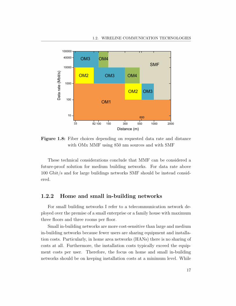
Figure 1.9: Optical backbone for home and small in-building networks
leads to a complicated consumer experience and high service and mainte-
nance costs. To provide a simplified and easily upgradable small building
network, a single common backbone infrastructure is required, as shown in
Fig. 1.9. High-speed wireline services are delivered to the home via fiber-
to-the-home (FTTH) or other technologies until the point of the gateway.
Then, the wireline services are distributed among the rooms through the op-
tical backbone. For this reason, the maximum data rate transferable over a
low-cost do-it-yourself POF network needs to be carefully investigated.
1.3 Wireless communication technologies
Wireless communications have experienced an ever-growing development
and commercial fortune in the last decade. Every day office and residential
users surf on the Internet through a wireless connection. In this thesis, with
wireless technologies I refer to radio and microwave transmission techniques
for personal communications. However, short-range wireless systems can
also exploit light as the information carrier, in particular visible light [19] or
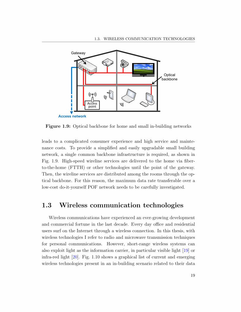
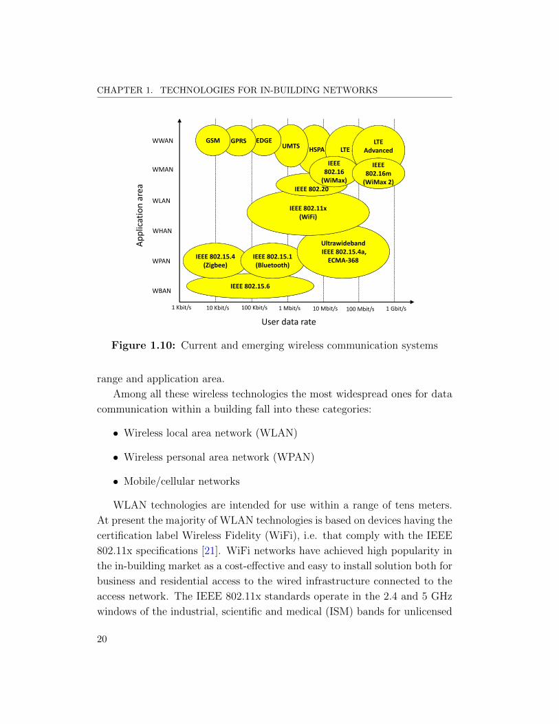
infra-red light [20]. Fig. 1.10 shows a graphical list of current and emerging
wireless technologies present in an in-building scenario related to their data
19
CHAPTER 1. TECHNOLOGIES FOR IN-BUILDING NETWORKS
WBAN
WPAN
WHAN
WLAN
WMAN
WWAN
1 Kbit/s 10 Kbit/s 100 Kbit/s 1 Mbit/s 10 Mbit/s 100 Mbit/s 1 Gbit/s
IEEE 802.15.6
IEEE 802.15.4
(Zigbee)
IEEE 802.15.1
(Bluetooth)
Ultrawideband
IEEE 802.15.4a,
ECMA-368
IEEE 802.11x
(WiFi)
HSPA
IEEE 802.20
LTE a a
LTE
Advanced
IEEE
802.16
(WiMax)
UMTSEDGEGPRSGSM
User data rate
Ap
pli
cati
on
are
a
( 2)
IEEE
802.16m
(WiMax 2)
Figure 1.10: Current and emerging wireless communication systems
range and application area.
Among all these wireless technologies the most widespread ones for data
communication within a building fall into these categories:
• Wireless local area network (WLAN)
• Wireless personal area network (WPAN)
• Mobile/cellular networks
WLAN technologies are intended for use within a range of tens meters.
At present the majority of WLAN technologies is based on devices having the
certification label Wireless Fidelity (WiFi), i.e. that comply with the IEEE
802.11x specifications [21]. WiFi networks have achieved high popularity in
the in-building market as a cost-effective and easy to install solution both for
business and residential access to the wired infrastructure connected to the
access network. The IEEE 802.11x standards operate in the 2.4 and 5 GHz
windows of the industrial, scientific and medical (ISM) bands for unlicensed
20

1.3. WIRELESS COMMUNICATION TECHNOLOGIES
use and guarantee throughput of 11 Mbit/s (802.11b), 54 Mbit/s (802.11a/g)
and 320 Mbit/s (802.11n) up to tens meters. There is also an active research
activity towards the 1 Gbit/s performance.
WPAN technologies are intended to interconnect devices around an in-
dividual person’s area, and thus their range is typically below 10 m. The
most known WPAN technologies are Bluetooth, Zigbee and ultra wideband
(UWB) technologies. All these technologies are also considered for wireless
body area network (WBAN), which are intended to connect wearable de-
vices within a range of few meters. UWB technologies have also applica-
tion in wireless home area network (WHAN), such as high-definition video
streaming or gaming, which is a special case of WLAN for residential use.
In contrast with WLAN and WPAN technologies which are wireless fixed
systems, mobile networks are intended to guarantee voice and data com-
munications between users in mobility. For this reason, a mobile network is
deployed by a mobile operator which requests a fee to its subscribers. Current
widespread mobile networks are based on the following technologies: Global
System for Mobile communications (GSM), Universal Mobile Telecommuni-
cations System (UMTS), Long Term Evolution (LTE) which use the licensed
radio frequency (RF) bands, such as the ones around 800-900, 1800-1900 and
2100 MHz [22]. These technologies are typically considered as wireless wide
area networks (WWANs), since they are used to cover a wide geographical
area. However, they are not only limited to WWANs. For example high speed
packet access (HSPA) was mainly deployed in metro areas. In this frame-
work, also wireless metropolitan area network (WMAN) technologies, such
as Worldwide Interoperability for Microwave Access (WiMAX), are start-
ing to support mobile users. Indeed, next-generation LTE–Advanced and
WiMAX 2 (IEEE 802.16m), identified as WirelessMAN–Advanced, are both
included in IMT-Advanced technologies of International Mobile Telecommu-
nications (IMT) [23], i.e. 4G mobile technologies, offering up to 100 Mbit/s
to users with high mobility and up to 1 Gbit/s to relatively fixed users. Since
in-building users are relatively fixed, the next-future challenge will be to be
really able to deliver 1 Gbit/s per user in an indoor scenario.
Differently from WPAN and WLAN technologies whose equipment is in
21
CHAPTER 1. TECHNOLOGIES FOR IN-BUILDING NETWORKS
Distribution fiber
Remote antenna unit
Base Station Hotel Mobile network
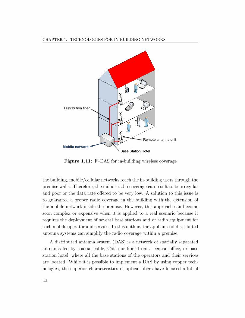
Figure 1.11: F–DAS for in-building wireless coverage
the building, mobile/cellular networks reach the in-building users through the
premise walls. Therefore, the indoor radio coverage can result to be irregular
and poor or the data rate offered to be very low. A solution to this issue is
to guarantee a proper radio coverage in the building with the extension of
the mobile network inside the premise. However, this approach can become
soon complex or expensive when it is applied to a real scenario because it
requires the deployment of several base stations and of radio equipment for
each mobile operator and service. In this outline, the appliance of distributed
antenna systems can simplify the radio coverage within a premise.
A distributed antenna system (DAS) is a network of spatially separated
antennas fed by coaxial cable, Cat-5 or fiber from a central office, or base
station hotel, where all the base stations of the operators and their services
are located. While it is possible to implement a DAS by using copper tech-
nologies, the superior characteristics of optical fibers have focused a lot of
22

1.3. WIRELESS COMMUNICATION TECHNOLOGIES
effort in the implementation of fiber DASs (F–DASs) [24]. Fig. 1.11 shows
an in-building F–DASs infrastructure. The base station hotel collects all
the wireless technologies and services of the telecom operators which are
distributed to the remote antenna units through optical links.
A F–DAS typically exploits the radio over fiber (RoF) technology, which
consists in the transport of the radio signal over a fiber-optic link [25]. RoF
systems can be classified into three categories depending on the way the radio
signal is transported on the fiber-optic link:
• the RF-over-fiber technique carries the radio signal in its original
band by modulating the light in an analog way. It guarantees complete
transparency and it is the approach typically used for all the radio
signals up to 10 GHz [26].
• the IF-over-fiber technique carries a down-converted version of the
original radio signal, which modulates the light in an analog way. Then,
the IF version of the radio signal is up-converted by electrical or optical
means at the remote antenna unit before being radiated into the air
[27]. This approach is typically used for the transport of high frequency
radio signals, such as at 60 GHz [28, 29] and at 75–100 GHz [30].
• the Digitized RF-over-fiber technique carries the radio signal in a
digital way. The radio signal is digitized according to the Nyquist pass-
band sampling theorem and its samples are transported by a digital
fiber-optic link [31]. This approach allows to employ the widespread
digital fiber links, but it is currently able to transport few narrow-band
radio carriers and with a higher cost compared to the RF-over-fiber
technique [32].
Since WLAN, WPAN and mobile/cellular systems use radio frequencies
below 5 GHz, the most convenient radio over fiber approach is constituted
by the RF-over-Fiber technique. The broadband capability of F–DAS based
on RF-over-Fiber technology allows the simultaneous transport of several
mobile/cellular systems and also of radio signal compliant with WLAN and
23

CHAPTER 1. TECHNOLOGIES FOR IN-BUILDING NETWORKS
WPAN standards. Moreover, due to the transparency to the radio format,
it provides future-proof upgradability.
However, it is important to underline that a F–DAS is not in principle
a low-cost system, hence the effective convenience of its implementation will
depend on the scenario where it is considered to be applied. For this reason,
as it was done in section 1.2, I differentiate the two cases of large-medium
and small in-building networks.
1.3.1 Large and medium in-building networks
Large and medium buildings are a case of in-building networks where
there can be a need for a multi-operator and multi-service wireless distribu-
tion system. Indeed, a shopping mall or a corporate building is a scenario
where a large number of low-mobility users ask to access the radio resources
simultaneously. Therefore, a F–DAS can be the solution to provide a good
radio coverage while keeping the cost per operator/service under control due
to the shared nature of a F–DAS infrastructure.
In large and medium in-building networks the wireless coverage through
F–DAS should be implemented by RF-over-fiber techniques. The capability
of multi-band and multi-operator is certainly of primary importance in large
and medium premises, together with a future-proofness of the implemented
network.
For this reason, as described in section 1.2.1, silica fibers are considered as
the proper transmission medium for the implementation of large and medium
in-building F–DASs. Moreover, also in this case both silica SMF and MMF
are good candidates depending on the application. In particular, SMF is a
mandatory choice for a new installation in large premises, while new silica
MMF can be used in medium buildings and existing MMF can be exploited
in both scenarios.
Several RF-over-fiber techniques can be employed for RF signals distri-
bution in combination with silica fibers. I differentiate them into three main
categories:
• Intensity modulation techniques
24
1.3. WIRELESS COMMUNICATION TECHNOLOGIES
• Phase or frequency modulation techniques
• Hybrid phase/frequency and intensity modulation techniques
Intensity modulation techniques are the simplest method to deliver a RF
signal and are realized via a direct or external modulation of a laser [33]. The
transmitter intensity modulation is usually connected with a receiver direct
detection achieved by a single photodiode [34], thus constituting an intensity
modulation – direct detection (IM–DD) system.
The IM–DD technique is applied to the great majority of current commer-
cial F–DAS systems for cellular signal distribution. Indeed, IM–DD systems
are able to deliver radio signals up to about 4–5 GHz for some hundreds of
meters of MMF and for tens kilometers of SMF [35, 36]. Strong limitations
come for higher radio frequencies or longer fiber link lengths due to modal
dispersion for MMF or chromatic dispersion for SMF [37, 38].
Phase or frequency modulation techniques consist in the modulation of
the phase/frequency of the light emitted by a laser [39]. The receiver can
be realized via a coherent scheme [40] or a phase to intensity modulation
converter scheme, realized by a dispersive medium [41], an optical frequency
discriminator [42] or an interferometric detection scheme [43, 44].
The main advantage of this technique with respect to intensity modulated
systems is the possibility to achieve a higher broadband RF link gain and
a lower noise, hence enhancing the dynamic-range of the analog optical link
[45]. Phase or frequency modulation techniques are yet at a research stage
and are not applied to commercial F–DAS systems, but they could turn
interesting in the future if the complexity and cost of the system will reduce.
Hybrid phase/frequency and intensity modulation techniques apply si-
multaneously an intensity and a phase/frequency modulation to the light
emitted by a laser. This scheme can be used to obtain particular modulation
format such as optical single sideband (SSB) modulation [46, 47]. The re-
ceiver can be based on several schemes depending on the modulation scheme
used. To demodulate the SSB signal a direct detection scheme is typically
employed [48].
The advantage of an hybrid phase/frequency and intensity modulation
25
CHAPTER 1. TECHNOLOGIES FOR IN-BUILDING NETWORKS
with respect to the previous two modulation schemes is not general. For op-
tical SSB the advantage is a major resilience to chromatic dispersion [46]. As
for phase/frequency modulation, hybrid modulation is presently not applied
to commercial F–DAS systems due to cost-issues and complexity.
Since the length of an in-building RF-over-fiber link does not exceed few
kilometers of length in large premises, and few hundreds of meters in medium
premises, the IM–DD technique is still an attractive solution for the distri-
bution of current and emerging WLAN, WPAN and cellular mobile signals
which are all below 3 GHz.
1.3.2 Home and small in-building networks
Contrary to large and medium premises, home and small in-building net-
works do not require to support a multi-operators multi-services wireless
distribution. Indeed, home or small office costumer pays a fee to just one
telecom operator. For this scenario several mobile operators have studied
the possibility to provide their customers with a femto-cell, or femto-node,
which is a simple, small and light cellular base station able to support 4-8
mobile users within a small office or a home environment, and connect to the
mobile network via the access network (e.g. a digital subscriber line (DSL)
connection) [49]. Moreover, also other types of technologies, such as WiFi,
do not require more than one or two access points to cover all the home or
small office network.
In this scenario a separate in-building F–DAS becomes then unneces-
sary. However, the possibility of using a fiber-optic infrastructure also for
the transport of wireless services to enhance the radio coverage can still be
convenient and attractive. Fig. 1.12 shows the scenario I am referring to.
All the home or small building services coming from the access network, the
satellite and wireless networks are centralized to the building gateway. These
services are then distributed to the different rooms through a converged opti-
cal backbone. The in-building users can have access to the different services
via a wireline or a wireless connection. Note that with respect to the sce-
nario presented in Fig. 1.9 where a wireless connection was enabled through
26

1.4. SUMMARY
Access network
Converged optical
backbone
Gateway
Figure 1.12: Converged optical backbone for home and small in-building
networks
a separate wireless access point, in Fig. 1.12 wireline and wireless services
are together delivered in the optical backbone and a simple RF front-end is
used to “tap” and irradiate the wireless services.
As stated in section 1.2.2, 1 mm diameter POF can be employed to im-
plement a low-cost optical backbone for wireline services. The possibility to
use 1 mm diameter POF to transport broadband wireless signal has been
demonstrated in [50]. However, the capability to support a converged sce-
nario needs still to be proved.
1.4 Summary
Fiber optic technologies and techniques for in-building networks have
been presented in this chapter. Section 1.1 described optical fibers based on
silica and polymer materials intended for indoor applications. For silica fiber,
the characteristics and classification of standardized single and multimode
fibers were reported, while for polymer fiber, plastic optical fibers based on
PMMA materials with a diameter of 1 mm were introduced. In particular,
27

CHAPTER 1. TECHNOLOGIES FOR IN-BUILDING NETWORKS
the standard POF, and 1 mm diameter PMMA POFs with a graded-index
or a multi-core profile were described.
Sections 1.2 and 1.3 presented the application of these fiber technologies
to in-building networks. Single and multimode silica fibers find appropriate
applications in large and medium building networks. For wireline services
distribution multimode fiber can reach 10 Gbit/s transmission up to 600 m,
while for 40 and 100 Gbit/s multimode fiber is limited to 150 m. For longer
distances and higher data rates single mode fiber should be considered. For
wireless services distribution the fiber distributed antenna system was intro-
duced as an enabling technology to enhance the radio coverage. An overview
of the state-of-the-art techniques was reported, and the cost-effectiveness of
the IM–DD RF-over-fiber technique for in-building networks has been under-
lined. My contribution on the potential achievement of this last technique
in conjunction with current optical components will be pointed out in chap-
ter 2 and 3 of this dissertation with reference to single and multimode fibers,
respectively.
For small building networks, such as small office and home scenarios, the
benefits of employing 1 mm diameter PMMA POFs were discussed. Indeed,
small building networks are very cost-sensitive due to the absence of cost
sharing. For this reason, silica fiber solutions are not widespread applica-
ble, while copper solutions, e.g. Cat-5, and power line communications are
typically utilized. However, with respect to copper solutions plastic optical
fibers have the advantage to be thinner and to be able to share electrical
wiring ducts. Commercial POF products support 100 Mbit/s transmission
up to 100 m, while prototypes have been reported for 1 Gbit/s transmission
up to 75 m on standard step-index POF. Only recently, multi-gigabit trans-
mission over 1 mm diameter PMMA POFs was demonstrated. In chapter 4
my research activity on multigigabit POF solutions will be described.
The possibility to exploit POF for a converged wireline and wireless
optical backbone in small-building scenarios has been discussed in subsec-
tion 1.3.2. With reference to this challenge, chapter 5 will report my contribu-
tion on converged short-range communications over 1 mm diameter PMMA
POF.
28

Chapter 2RoF systems over SMF
for in-building F–DAS
In this chapter studies on state-of-the-art F–DAS links employing SMF
and directly modulated distributed feed-back (DFB) lasers are reported. An
efficient and accurate model evaluating the performance of the transmission
of real radio signals in these links is presented. Finally, transmission experi-
ments employing UMTS and WiMAX signals will be presented and compared
with simulated results.
2.1 Developed theoretical model
In this section I present the modeling of the different components of our
system. The scope of this activity is to obtain a numerical model which is
able to calculate some important link performance parameters while keeping
the simulation time and the complexity under control.
This chapter is based on the results published in P1., P9., and P14.
29

CHAPTER 2. ROF SYSTEMS OVER SMF FOR IN-BUILDING F–DAS
2.1.1 Directly modulated laser
2.1.1.1 Intensity modulation and transmitter non-linearities
An intensity modulation produced by the direct modulation of a laser
diode gives rise to an optical power P (t) that can be written as,
P (t) = P0 + ηTXi(t) + α2i2(t) + α3i
3(t) (2.1)
where P0 is the optical power, i(t) is the electrical modulating current, ηTXis the conversion efficiency of the laser diode, α2 and α3 are the undesired
non-linear coefficients of the second and third order [51].
The electrical modulating current i(t) is a radio signal. It can be written
as a generic pass-band signal, i.e. a carrier modulated in amplitude and in
phase. An equivalent representation is to consider it as a sum of two orthog-
onal carriers modulated in amplitude at the same frequency, mathematically
cos(.) and sin(.) functions of the same argument,
i(t) = IRF [I(t) cos (2πfct)−Q(t) sin (2πfct)] = IRF s(t) (2.2)
where IRF and fc are the amplitude and the frequency of the carrier, respec-
tively. I(t) and Q(t) are the in-phase and in-quadrature components, which
contain the signal information.
In (2.2) I introduce the normalized modulating signal s(t). There are
two possible normalization choices. The first one is to normalize s(t) to its
maximum value, i.e. max(|s(t)|) = 1. This is the common choice when
considering digital baseband transmission, where the peak-to-peak electrical
voltage or current is of primary importance, and it can measured via an
oscilloscope. The second choice is to normalize the mean square value of
s(t) to get the same value of a sinusoidal tone, i.e. 〈s2(t)〉 = 1/2. Here, I
took this second choice since I consider the analog transmission of a radio
signal, where the main parameter under study is the electrical power, which
is typically measured by a spectrum analyzer.
30

2.1. DEVELOPED THEORETICAL MODEL
Using (2.2) in (2.1) it is,
P (t) = P0
[1 +
ηTXIRFP0
s(t) +α2I
2RF
P0
s2(t) +α3I
3RF
P0
s3(t)
]=
= P0
[1 +mIs(t) + a2m
2Is
2(t) + a3m3Is
3(t)]
(2.3)
In (2.3) I introduce the optical modulation index (OMI), mI = ηTXIRF/P0.
Similarly, I define the second and third order coefficients a2 = α2P0/η2TX and
a3 = α3P20 /η
3TX .
It is possible to generalize (2.3) to the transmission of more than one
radio signal,
P (t) = P0
1 +∑k
mksk(t) + a2
(∑k
mksk(t)
)2
+ a3
(∑k
mksk(t)
)3
(2.4)
where sk(t) is the kth normalized modulating signal and mk is its OMI.
Starting from (2.4) and using a two-tone test it is possible to determine
experimentally the non-linear coefficients a2 and a3. In this case, it is,
P (t) = P0 [1 +m (cos(2πfc,1t) + cos(2πfc,2t)) +
+a2m2 (cos(2πfc,1t) + cos(2πfc,2t))
2 +
+a3m3 (cos(2πfc,1t) + cos(2πfc,2t))
3] (2.5)
To calculate a2 we look at the ratio between the power of one of the two
carriers at fc,1 or fc,2, identified as C, and the power of the second order
intermodulation distorsion (IMD) at fc,1 + fc,2, identified as IMD2,
C
IMD2=
1
a22m
2(2.6)
Since C/IMD2 changes with the input power CIN , I will relate a2 to
the input intercept point of the second order (IIP2) [52], that is a quantity
invariant with respect to CIN . Indeed, it is IIP2 = C/IMD2 +CIN . Then,
it is,
a2 =P0
ηTX
√RL
2 · IIP2(2.7)
31

CHAPTER 2. ROF SYSTEMS OVER SMF FOR IN-BUILDING F–DAS
In (2.7) I applied the definition of mI and CIN = RL/2 · I2RF , where RL
is the load resistance, typically 50 Ω.
Similarly, it is possible to calculate a3 from the input intercept point of
the third order (IIP3),
a3 =
(P0
ηTX
)22RL
3 · IIP3(2.8)
2.1.1.2 Frequency chirping
When a laser is directly modulated in intensity it also produces an un-
wanted frequency and phase modulation, called frequency chirping. The
frequency deviation is equal to,
∆f(t) =α
4π
(d (ln(P (t))
dt+ κP (t)
)(2.9)
α is the line-width enhancement factor and κ is the adiabatic frequency chirp
scaling factor [53].
Substituting (2.4) in (2.9) and approximating at the first order we have,
∆f(t) ≈∑k
mk ·α
4π
(dsk(t)
dt+ κP0sk(t)
)=∑k
∆fk(t) (2.10)
The derivative of sk(t) in (2.10) is equal to,
dsk(t)
dt=
(dIk(t)
dt− 2πfc,kQk(t)
)cos (2πfc,kt) +
+
(dQk(t)
dt− 2πfc,kIk(t)
)sin (2πfc,kt) (2.11)
Since sk(t) are pass-band signal, Ik(t) and Qk(t) are slow varying signals
compared to the radio carrier at frequency fc,k. Then, applying the slowly
varying envelope approximation [54], it is |dIk(t)/dt| 2πfc,k|Qk(t)| and
|dQk(t)/dt| 2πfc,k|Ik(t)|. Thus, (2.11) can be approximated as,
dsk(t)
dt≈ −2πfc,k (Qk(t) cos (2πfc,kt) + Ik(t) sin (2πfc,kt)) (2.12)
32
2.1. DEVELOPED THEORETICAL MODEL
It is possible to proceed further to get,
d2sk(t)
dt2≈ −(2πfc,k)
2 (Ik(t) cos (2πfc,kt)−Qk(t) sin (2πfc,kt)) =
= −(2πfc,k)2sk(t) (2.13)
From (2.13) we get then,∫ t
−∞sk(τ)dτ ≈ − 1
(2πfc,k)2
dsk(t)
dt=
=1
2πfc,k(Qk(t) cos (2πfc,kt) + Ik(t) sin (2πfc,kt))(2.14)
From this last result we can calculate the phase variation, ϕk(t), induced
by the frequency deviation ∆fk(t).
ϕk(t) = 2π
∫ t
−∞∆fk(τ)dτ = mk ·
α
2
(sk(t) + κP0
∫ t
−∞sk(τ)dτ
)=
= mk ·α
2
[(Ik(t) +
κP0
2πfc,kQk(t)
)cos (2πfc,kt)−
−(Qk(t)−
κP0
2πfc,kIk(t)
)sin (2πfc,kt)
](2.15)
To determine experimentally the factors α and κ, I employed the delayed
self-homodyne technique [55, 56]. In this method the laser source is directly
modulated with a sinusoidal tone, thus generating an intensity and a fre-
quency/phase modulation. To measure the frequency/phase modulation a
phase-to-intensity conversion is obtained with an interferometer. In the case
of a modulation signal equal to s(t) = cos(2πfct) the phase ϕ(t) becomes,
ϕ(t) = m · α2
[cos (2πfct) +
κP0
2πfcsin (2πfct)
]=
= m · α2
√1 +
(κP0
2πfc
)2
· sin[2πfct+ arctan
(2πfcκP0
)]=
= p sin [2πfc (t− ν)] (2.16)
The self-homodyne technique is able to measure the phase index p to-
gether with the modulation index m, from which we can recover the intrinsic
33

CHAPTER 2. ROF SYSTEMS OVER SMF FOR IN-BUILDING F–DAS
characteristic of the laser p/m at several modulation frequency fc.
p
m=α
2
√1 +
(κP0
2πfc
)2
(2.17)
From the values of p/m determined at different values of the modulation
frequency, fc, it is possible to extrapolate the characteristic quantities α and
κ. Since typical values for κ are between 2 and 10 GHz/mW while they are
between 4 and 10 mW for P0, the ratio κP0/2πfc 1 for modulation fre-
quencies well below the resonance frequency of the laser, which is typically
ranging from 4 to 10 GHz for laser intended for analog applications below
10 GHz [57]. Equivalently this means that the frequency modulation compo-
nent (proportional to κ) tends to overcome the phase modulation component.
For this reason, it is a common practice to consider a frequency modulation
index Kf in (MHz/mA) instead of the phase modulation index p/m. The
two quantities are related by,
∆f(t) = pfc cos [2πfc (t− ν)] = KfIRF cos [2πfc (t− ν)] (2.18)
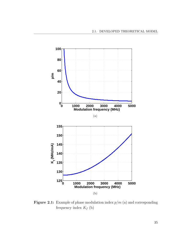
In Fig. 2.1 it is shown a comparison of the values of p/m and Kf versus
the modulating frequency fc for typical values of the quantities α, κ and P0.
It can be observed that the frequency index Kf can be considered almost
constant for modulation frequencies typical of mobile radio communications
(fc ranging from 700 to about 2700 MHz), while the phase index p/m strongly
varies especially in the radio frequencies region. Indeed, for frequencies well
below the resonance frequencies Kf is not so depending on the modulation
frequency fc. In the following the transmitter frequency chirp characteristic
will be often referred through its frequency index Kf .
2.1.1.3 Electrical field
With the mathematical model of the laser intensity modulation and fre-
quency chirping it is possible to express the electrical field E(t),
E(t) =√
2ZP (t) · exp
2π
[f0t+
∫ t
−∞∆f(τ)dτ
]=
= ELP (t) exp 2πf0t (2.19)
34
2.1. DEVELOPED THEORETICAL MODEL
0 1000 2000 3000 4000 50000
20
40
60
80
100
Modulation frequency (MHz)
p/m
(a)
0 1000 2000 3000 4000 5000125
130
135
140
145
150
155
Modulation frequency (MHz)
Kf (
MH
z/m
A)
(b)
Figure 2.1: Example of phase modulation index p/m (a) and corresponding
frequency index Kf (b)
35
CHAPTER 2. ROF SYSTEMS OVER SMF FOR IN-BUILDING F–DAS
where Z is the wave impedance [58] and f0 is the central emission frequency
of the laser.
In (2.19) I defined the complex-envelope or equivalent low-pass electrical
field ELP (t). Using (2.4), (2.10) and (2.15) it is,
ELP (t) = E0
√√√√1 +∑k
mksk(t) + a2
(∑k
mksk(t)
)2
+ a3
(∑k
mksk(t)
)3
·
· exp
∑k
ϕk(t)
(2.20)
E0 =√
2ZP0 is the electrical field amplitude, and ϕk(t) is the phase modu-
lation generated by the kth modulating signal.
Equations (2.19) and (2.20) allow writing the electrical field generated by
the direct modulation of a laser source by a set of radio signals, identified by
their in-phase and in-quadrature components and carrier frequencies.
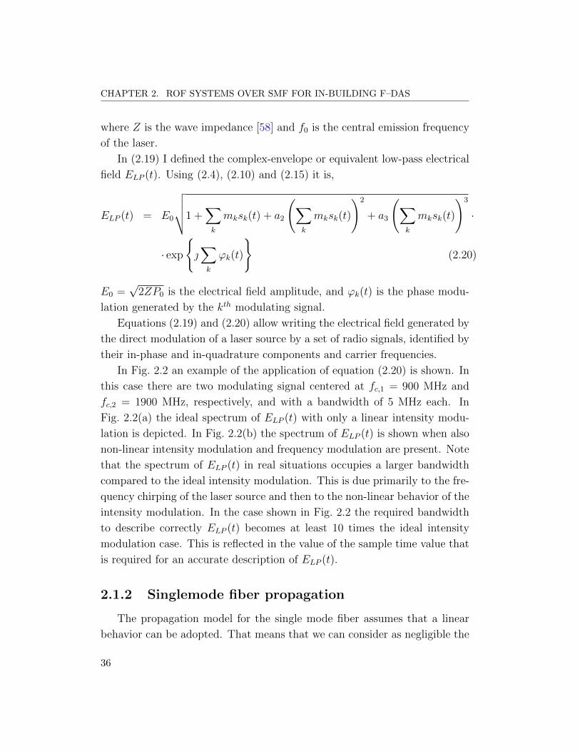
In Fig. 2.2 an example of the application of equation (2.20) is shown. In
this case there are two modulating signal centered at fc,1 = 900 MHz and
fc,2 = 1900 MHz, respectively, and with a bandwidth of 5 MHz each. In
Fig. 2.2(a) the ideal spectrum of ELP (t) with only a linear intensity modu-
lation is depicted. In Fig. 2.2(b) the spectrum of ELP (t) is shown when also
non-linear intensity modulation and frequency modulation are present. Note
that the spectrum of ELP (t) in real situations occupies a larger bandwidth
compared to the ideal intensity modulation. This is due primarily to the fre-
quency chirping of the laser source and then to the non-linear behavior of the
intensity modulation. In the case shown in Fig. 2.2 the required bandwidth
to describe correctly ELP (t) becomes at least 10 times the ideal intensity
modulation case. This is reflected in the value of the sample time value that
is required for an accurate description of ELP (t).
2.1.2 Singlemode fiber propagation
The propagation model for the single mode fiber assumes that a linear
behavior can be adopted. That means that we can consider as negligible the
36
2.1. DEVELOPED THEORETICAL MODEL
−20 −15 −10 −5 0 5 10 15 201E−10
1E−8
1E−6
1E−4
1E−2
1E0
Frequency (GHz)
Spe
ctru
m o
f ide
al E
LP(t
)
(a)
−20 −15 −10 −5 0 5 10 15 201E−10
1E−8
1E−6
1E−4
1E−2
1
Frequency (GHz)
Spe
ctru
m o
f ELP
(t)
(b)
Figure 2.2: Spectrum of ELP (t) in the case of an ideal intensity modulation
(a) and in a real situation (b). The modulating signals are cen-
tered at fc,1 = 900 and fc,2 = 1900 MHz and with a bandwidth
of 5 MHz
37

CHAPTER 2. ROF SYSTEMS OVER SMF FOR IN-BUILDING F–DAS
effects of the fiber non-linearities, and that an impulse response or a transfer
function can be defined [3]. In particular, the transfer function H(f, z) is,
H(f, z) = e−(α(f)+β(f))z (2.21)
α(f) and β(f) are, respectively, the fiber attenuation and propagation coef-
ficient per unit of length. z is the fiber length and f is the optical frequency.
Since this model is applied to a single wavelength source as described in
subsection 2.1.1, the transfer function in (2.21) can be approximated around
the optical central frequency f0 of the source by,
H(f, z) = e−α(f0)z · e−
(β(f0)+τg2π(f−f0)− c
4πf20D(2π(f−f0))2
)z
(2.22)
where τg is the fiber group delay per unit of length, c is the light velocity,
and D is the fiber chromatic dispersion in s/m2.
Since the electrical field in (2.19) is an optical pass-band signal, the optical
transfer function H(f, z) in (2.21) can be replaced by an equivalent low-pass
transfer function, H0(f, z), which is applied to ELP (t) of (2.20). Moreover
it is possible to neglect the terms containing β(f0) and τg since they simply
provide a phase shift to the optical carrier and a time delay to the complex-
envelope. It is then,
H0(f, z) = e−α(f0)z · e c
4πf20D(2πf)2z
(2.23)
where f = f − f0 is the frequency distance from the optical carrier.
The corresponding time impulse response is
h0(t, z) = e−α(f0)z ·√
π
ϑ· e
π2
ϑt2 (2.24a)
ϑ = D · z · πcf 2
0
(2.24b)
Theoretically the impulse response in (2.24a) can be employed to de-
scribe numerically the fiber propagation. However, the infinite time length
of h0(t) does not allow this approach. For this reason the linear fiber propa-
gation is usually modeled in the frequency domain by multiplying the Fourier
38

2.1. DEVELOPED THEORETICAL MODEL
Transform of ELP (t) with the transfer function H0(f, z) and with an inverse
Fourier transform of the obtained result. This model is general and correct,
but it becomes heavy in term of resources and time for increasing size of the
samples which describes ELP (t), i.e. decreasing sample time and/or increas-
ing simulation time. In this framework, a numerical method employing the
convolution of a short impulse response with respect to the signal ELP (t) can
bring advantages in terms of time simulation and resources needed.
Therefore, I aim to determine an impulse response which, contrary to
h0(t, z), exhibits a finite time length. My starting point is to note that the
complex-envelope ELP (t) has a finite double-side bandwidth B. For our aim
H0(f, z) can then also be considered limited to this bandwidth. Therefore it
is possible to assume,
H0,B(f, z) = H0(f, z) ·WB(f) (2.25)
where WB(f) is a window with the property to limit the transfer function
bandwidth around B.
Among the infinite choices for this window I choose the following,
W(f)
=
1∣∣f ∣∣ ≤ B/2
e−(|f|−B/2
∆f
)2 ∣∣f ∣∣ > B/2(2.26)
where ∆f is a window parameter
The main advantage of this window function is that the impulse response
obtained through the inverse Fourier transform of H0,B(f, z) can be expressed
by an analytical formula. After some calculations it is,
h0,B(t, z) = e−α(f0)z · (hB (t, z) + h+ (t, z) + h− (t, z)) (2.27a)
hB (t, z) = e−π2
ϑt ·√π
ϑ
[1
2erfz
(√ϑ
B
2+
π√ϑt
)−
− 1
2erfz
(−
√ϑ
B
2+
π√ϑt
)](2.27b)
39
CHAPTER 2. ROF SYSTEMS OVER SMF FOR IN-BUILDING F–DAS
h± (t, z) =
√π · erfcz (u± (z))
2√
1
∆f2 − ϑ
·
· exp
(±πt+ B
2∆f2
)2
1
∆f2 − ϑ
− B2
4∆f2
(2.27c)
u±(z) =B
2·√
1
∆f2 − ϑ−
±πt+ B
2∆f2√
1
∆f2 − ϑ
(2.27d)
the quantity ϑ is the same as in (2.24b), while erfz and erfcz are the error
function and the complementary error function, respectively, evaluated for a
complex input argument [59].
Fig. 2.3 shows a comparison between the real and imaginary components
of h0(t, z) and h0,B(t, z). In this example f0 = 193.4 THz, α(f0) = 0 dB/km,
D = 16 ps/nm/km, z = 50 km, B = 28 GHz, ∆f = 3 GHz.
As depicted in Fig. 2.3, the impulse response h0,B(t, z) is a energy finite
function, which goes to zero for increasing time (t). The key to diminish
the computation complexity and time with respect to the frequency domain
approach is to limit together with the bandwidth also its time-width. To this
purpose, the length of h0,B(t, z) can be fixed to that interval whose values
are above a relative threshold, th, with respect to the maximum absolute
value. Referring to the case considered to obtain Fig. 2.3, taking a threshold
th = 10−4 the time-width of the impulse response is 1.6 ns for z = 10 km and
2.1 ns for z = 50 km. Taking a threshold th = 10−3 the time-width reduces
to 0.75 ns and 0.95 ns for z = 10 km and z = 50 km, respectively.
From a numerical point of view, the time-width reduction of the impulse
response reflects in a faster computation of the convolution of ELP (t) with
h0,B(t, z). In relation with the previous numerical example, choosing a sam-
pling time ∆t = 1/(2(B+ 2∆f)) = 25 ps the impulse response is constituted
by 65 and 85 samplings in the case of z = 10 km and z = 50 km, respectively,
for th = 10−4. For th = 10−3 the samples reduces to 31 and 39. The samples
required for ELP (t) depend instead on the simulation time. In the case of
40

2.1. DEVELOPED THEORETICAL MODEL
−0.5 −0.25 0 0.25 0.5−1.5
−1
−0.5
0
0.5
1
1.5x 10
10
time (ns)
Impu
lse
resp
onse
rea
l par
t
(a) Real component
−0.5 −0.25 0 0.25 0.5−1.5
−1
−0.5
0
0.5
1
1.5x 10
10
time (ns)
Impu
lse
resp
onse
imag
inar
y pa
rt
(b) Imaginary component
Figure 2.3: Comparison of the real (a) and imaginary (b) components of an
example of the bandwidth unlimited impulse response h0(t, z)
(green) with the corresponding bandwidth limited impulse re-
sponse h0,B(t, z) (blue)
41
CHAPTER 2. ROF SYSTEMS OVER SMF FOR IN-BUILDING F–DAS
500 µs of simulated time the samples of ELP (t) are 20 million which is in-
finitely more than the 30-90 samples required for the impulse response. Thus
the numerical convolution between ELP (t) and h0,B(t, z) becomes identical
to a filtering of ELP (t) performed by a finite impulse response (FIR) filter
with 30-90 taps. This leads to an efficient computation of the convolution
algorithm in term of memory resources and simulation time.
2.1.3 Photodiode model
The photodiode model describes the envelope detection performed by
the photodiode. If it is able to receive all the spectrum components within
the system bandwidth B, then the received current iout(t) can simply be
calculated by,
iout (t, z) = R · |ELP (t) ∗ h0,B(t, z)|2
2Z(2.28)
where R is the photodiode responsivity and the notation ∗ stands for the
convolution operation.
Fig. 2.4 displays numerical results obtained by applying the model de-
scribed in this section. The input field and the fiber impulse response are
the same shown in Fig. 2.2(b) and Fig. 2.3(a)–(b), respectively. In Fig. 2.4(a)
the spectrum of the current iout(t) in the case of no fiber propagation is shown.
In this case what is shown is the spectrum of |ELP (t)|2, which is due to the
linear and non-linear intensity modulation. Fig. 2.4(b) shows the spectrum
of the current iout(t) after a fiber length z = 50 km. Comparing Fig. 2.4(a)
and 2.4(b), it can be observed that higher order harmonics are generated by
fiber propagation. For this reason, some important performance parameters
need to be taken under consideration to define the signal quality transmis-
sion. In the next section experimental results of radio signals transmission on
IM–DD links employing singlemode fiber will be shown and compared with
the simulation predictions obtained by the application of the model described
in this section.
42

2.1. DEVELOPED THEORETICAL MODEL
−10 −5 0 5 10
10−6
10−4
10−2
100
Frequency (GHz)
Spe
ctru
m o
f iou
t(t)
for
z =
0 km
(a) z = 0 km
−10 −5 0 5 10
10−6
10−4
10−2
100
Frequency (GHz)
Spe
ctru
m o
f iou
t(t)
for
z =
50 k
m
(b) z = 50 km
Figure 2.4: Comparison of the spectrum of iout(t) for a fiber length z = 0 km
(a) and for z = 50 km (b)
43
CHAPTER 2. ROF SYSTEMS OVER SMF FOR IN-BUILDING F–DAS
2.2 Experimental and theoretical results
In this section the experimental activity performed on RoF IM–DD links
employing singlemode fiber is presented. The aim of this work was to verify
the adjacent channel leakage ratio (ACLR) degradation due to RoF TX, RX
and fiber propagation in a dual standard transmission. After the introduction
on the experimental setup, experimental results obtained with different RoF
TXs will be shown and compared with simulation results obtained with the
numerical model described in section 2.1.
2.2.1 Experimental setup
The experimental setup is shown in Fig. 2.5. Two RF signals were com-
bined and transmitted on the RoF IM–DD link. The RF signals were gen-
erated by two Agilent N5182A MXG vector signal generators (VSGs) and
were compliant with the UMTS and WiMAX standards. The UMTS carrier
frequency was fixed in the 2110–2170 MHz downlink (DL) band [60] and the
WiMAX carrier frequency in the 2500–2690 MHz DL band [61], which are
both IMT-2000 allocated bands. The output power of the two VSGs was
kept at a value which gave the highest level of ACLR directly from the in-
strument. Since this value was below −10/−5 dBm, two highly-linear power
amplifiers (PAs) were needed to increase the power levels to highest values.
The combination of the two signals was applied to three different RoF
TXs based on directly modulated DFB laser diodes (LDs). The emission
wavelength, λ0, of the RoF TXs were around 1550 nm (C band) and the
optical power was +10 dBm. The other measured and modeled parameters
are listed in Tab. 2.1. The output pig-tail of the RoF TX was connected to
an optical variable attenuator, followed by different spans of SMF to reach a
total length ranging from few meters to 50 km. All the fiber spans were of
standard SMF compliant with ITU-T G.652 recommendation [4]. Therefore,
fiber chromatic dispersion was modeled according to the formula in [4],
D (λ0) = D1550 + S1550 (λ0 − 1550) (2.29)
44
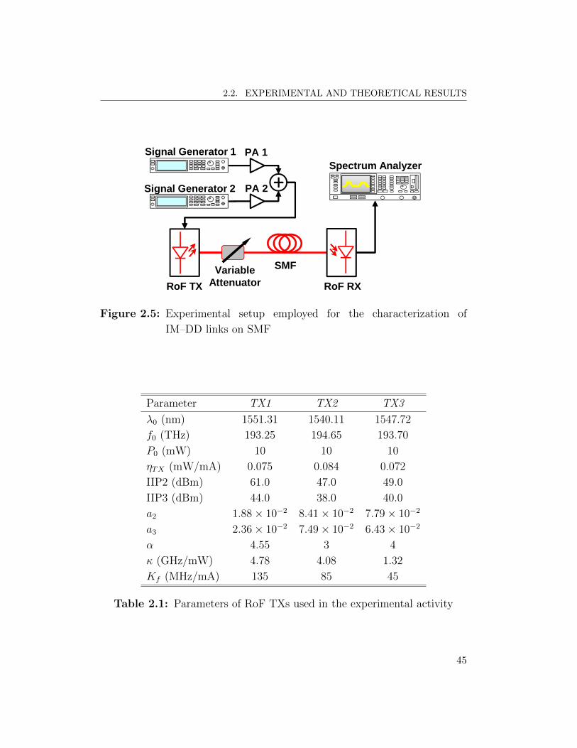
2.2. EXPERIMENTAL AND THEORETICAL RESULTS
VariableAttenuator
SMF
Spectrum Analyzer
RoF TX RoF RX
Signal Generator 1 PA 1
PA 2 +Signal Generator 2
Figure 2.5: Experimental setup employed for the characterization of
IM–DD links on SMF
Parameter TX1 TX2 TX3
λ0 (nm) 1551.31 1540.11 1547.72
f0 (THz) 193.25 194.65 193.70
P0 (mW) 10 10 10
ηTX (mW/mA) 0.075 0.084 0.072
IIP2 (dBm) 61.0 47.0 49.0
IIP3 (dBm) 44.0 38.0 40.0
a2 1.88× 10⁻² 8.41× 10⁻² 7.79× 10⁻²
a3 2.36× 10⁻² 7.49× 10⁻² 6.43× 10⁻²
α 4.55 3 4
κ (GHz/mW) 4.78 4.08 1.32
Kf (MHz/mA) 135 85 45
Table 2.1: Parameters of RoF TXs used in the experimental activity
45
CHAPTER 2. ROF SYSTEMS OVER SMF FOR IN-BUILDING F–DAS
D1550 is the dispersion coefficient at 1550 nm (ps/nm × km) and S1550
is the dispersion slope coefficient at 1550 nm (ps/nm2 × km). Accord-
ing to the representative value in [4], I set D1550 = 17 ps/nm × km and
S1550 = 0.056 ps/nm2 × km. The corresponding dispersion values at the
three different operating wavelengths of the RoF TXs were 17.07, 16.45, and
16.87 ps/nm× km for TX1, TX2 and TX3, respectively.
The variable attenuator was used to guarantee the same optical power
at the output of the fiber with the aim to set the noise level of the link in
all the configurations reported. In particular, the total optical attenuation
including optical connectors was set to 13.5 dBm.
Finally, the fiber was connected to a RoF RX based on a InGaAs positive-
intrinsic-negative (PIN) photodiode followed by a trans-impedance amplifier
(TIA). The electrical output port of the RoF RX was connected to an
Agilent N9020A MXA vector signal analyzer (VSA) used to measure the
ACLR in the two bands. The RoF RX was modeled by (2.28) assuming
that receiver non-linearities were negligible compared to the ones induced by
the transmitter and by the optical link. This assumption was well consistent
since the received optical power was quite low due to the fixed optical budget
of 13.5 dBm. Hence, the TIA worked in his linear region.
To explain graphically the meaning of ACLR, Fig. 2.6 shows an example
of ACLR test on a UMTS signal centered at 2140 MHz. The nominal TX-
channel bandwidth is 3.84 MHz and the channel spacing is 5 MHz. Therefore,
the adjacent channels are centered at 2140± 5 MHz, and the alternate chan-
nels at 2140± 10 MHz. The nominal channel bandwidth is always 3.84 MHz
for the adjacent and alternate channels. The ACLR is defined as the ratio
between the power in the adjacent channel and the power in the transmitted
channel. It is expressed in dB or dBc (dB carrier).
In the same way, the ACLR test for a WiMAX signal set the nominal
channel bandwidth to 9.5 MHz with a carrier spacing of 10 MHz. In my
case, the signal was centered at 2675 MHz, thus the adjacent channels were
centered at 2675± 10 MHz.
46

2.2. EXPERIMENTAL AND THEORETICAL RESULTS
Ref -13.8 dBm Att 10 dB*
*
*
RBW 30 kHzVBW 300 kHzSWT 100 ms*
Center 2.1399998 GHz Span 25.5 MHz2.55 MHz/
-110
-100
-90
-80
-70
-60
-50
-40
-30
-20
Tx Channel W-CDMA 3GPP FWD
Bandwidth 3.84 MHz Power -9.32 dBm Adjacent Channel
Bandwidth 3.84 MHz Lower -56.59 dB Spacing 5 MHz Upper -53.02 dB
Alternate Channel
Bandwidth 3.84 MHz Lower -65.08 dB Spacing 10 MHz Upper -64.94 dB
Adjacent
Channel
Alternate
Channel
TX Channel Adjacent
Channel
Alternate
Channel
Figure 2.6: Example of ACLR test for an UMTS–compliant signal
2.2.2 Experimental results and comparisons
The purpose of the experimental activity was to study the mutual distor-
tions generated by the simultaneous transmission of the two different radio
signals. Hence, the ACLR test was performed for different pairs of modula-
tion indexes of the two signals, namely m1 and m2. I chose the three discrete
values 0.1, 0.2 and 0.3 for m1 and m2 and it was possible to consider all the
combinations with m1 +m2 ≤ 0.4 avoiding LD clipping.
From Fig. 2.7 to Fig. 2.9 the most significant results are shown for the
three RoF TXs. In subfigures (a) three different curves of ACLR for the
UMTS signal are shown versus increasing fiber length. Each curve corre-
sponds to a different value of the modulation index of the WiMAX signal,
m2, varying from 0.1 to 0.3, while the modulation index of the UMTS signal,
m1, was kept at 0.1. Similarly, subfigures (b) show three different curves of
ACLR for the WiMAX signal with m2 constant at 0.1 and m1 varying from
0.1 to 0.3. The only exception are Fig. 2.9(a) and Fig. 2.9(b) where the only
47
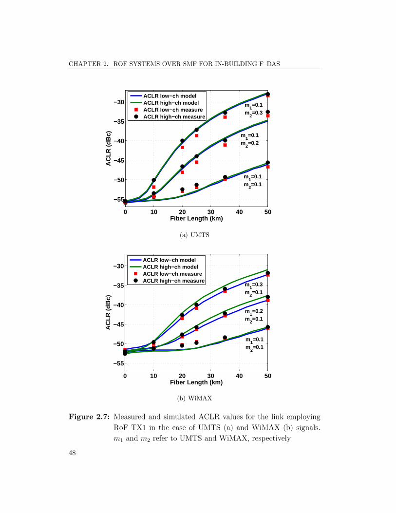
CHAPTER 2. ROF SYSTEMS OVER SMF FOR IN-BUILDING F–DAS
0 10 20 30 40 50
−55
−50
−45
−40
−35
−30
Fiber Length (km)
AC
LR (
dBc)
ACLR low−ch modelACLR high−ch modelACLR low−ch measureACLR high−ch measure
m1=0.1
m2=0.3
m1=0.1
m2=0.2
m1=0.1
m2=0.1
(a) UMTS
0 10 20 30 40 50
−55
−50
−45
−40
−35
−30
Fiber Length (km)
AC
LR (
dBc)
ACLR low−ch modelACLR high−ch modelACLR low−ch measureACLR high−ch measure
m1=0.3
m2=0.1
m1=0.2
m2=0.1
m1=0.1
m2=0.1
(b) WiMAX
Figure 2.7: Measured and simulated ACLR values for the link employing
RoF TX1 in the case of UMTS (a) and WiMAX (b) signals.
m1 and m2 refer to UMTS and WiMAX, respectively
48
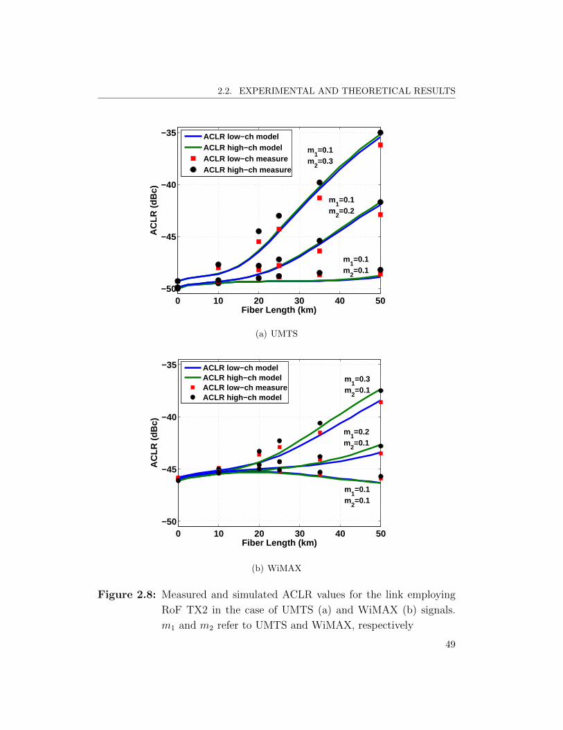
2.2. EXPERIMENTAL AND THEORETICAL RESULTS
0 10 20 30 40 50−50
−45
−40
−35
Fiber Length (km)
AC
LR (
dBc)
ACLR low−ch modelACLR high−ch modelACLR low−ch measureACLR high−ch measure
m1=0.1
m2=0.3
m1=0.1
m2=0.2
m1=0.1
m2=0.1
(a) UMTS
0 10 20 30 40 50−50
−45
−40
−35
Fiber Length (km)
AC
LR (
dBc)
ACLR low−ch modelACLR high−ch modelACLR low−ch measureACLR high−ch model
m1=0.1
m2=0.1
m1=0.2
m2=0.1
m1=0.3
m2=0.1
(b) WiMAX
Figure 2.8: Measured and simulated ACLR values for the link employing
RoF TX2 in the case of UMTS (a) and WiMAX (b) signals.
m1 and m2 refer to UMTS and WiMAX, respectively
49

CHAPTER 2. ROF SYSTEMS OVER SMF FOR IN-BUILDING F–DAS
0 10 20 30 40 50
−54
−52
−50
−48
−46
−44
−42
Fiber Length (km)
AC
LR (
dBc)
ACLR low−ch modelACLR high−ch modelACLR low−ch measureACLR high−ch model
m1=0.1
m2=0.3
(a) UMTS
0 10 20 30 40 50
−54
−52
−50
−48
−46
−44
−42
Fiber Length (km)
AC
LR (
dBc)
ACLR low−ch modelACLR high−ch modelACLR low−ch modelACLR high−ch model
m1=0.3
m2=0.1
(b) WiMAX
Figure 2.9: Measured and simulated ACLR values for the link employing
RoF TX3 in the case of UMTS (a) and WiMAX (b) signals.
m1 and m2 refer to UMTS and WiMAX, respectively
50

2.2. EXPERIMENTAL AND THEORETICAL RESULTS
pairs m1 = 0.1 and m2 = 0.3 (a), m1 = 0.3 and m2 = 0.1 (b) are shown since
the other combinations give rise to similar curves that are not reported here
for readability of the two graphs.
Note that the ACLR values for short distances differ in the two cases of
UMTS and WiMAX signals. This is caused by the different integration band-
width in the two cases. UMTS nominal bandwidth is fixed to 3.84 MHz and
WiMAX nominal bandwidth to 9.5 MHz. Hence, when distortions generated
in the adjacent channels caused by the optical link are negligible compared
to noise, the power in the adjacent channel increases with integration band-
width. In this particular case the difference is 10× log10 (9.5/3.84) = 3.9 dB,
that is observed in Fig. 2.7, 2.8 and 2.9.
Another behavior for short distances to be observed is that ACLR values
are practically independent from m2 (a) or m1 (b). This means that the
non-linear characteristics of the RoF TX does not produce a considerable
cross-effect on ACLR. The only exception is the case m1 = 0.1 and m2 = 0.3
in Fig. 2.8(a). This is due to the worse non-linearity characteristics of RoF
TX2 with respect to the other transmitters as shown in Tab. 2.1.
For increasing fiber length the common behavior is the increase of ACLR
in every curve in Fig. 2.7, 2.8 and 2.9. The only exception is the curve
corresponding to m1 = 0.1 and m2 = 0.1 in Fig. 2.8(b). This peculiar
effect is not due to a decrease of the power in the adjacent channel, but
to a relative increase of the power in the received TX-channel caused by a
phase-to-intensity conversion produced by fiber chromatic dispersion. This is
exactly the same reason which produces a higher relative increase of power in
the adjacent channels with respect to the TX-channel as can be observed in
all the other cases in Fig. 2.7, 2.8 and 2.9. However, when the relative increase
of power in the adjacent channel remains under the noise floor the ACLR
variations are driven by the relative change of power in the TX-channel.
This is the case of the curve corresponding to m1 = 0.1 and m2 = 0.1 in
Fig. 2.8(b).
Pointing the attention in all the curves with m1 = 0.1 and m2 = 0.3 in
Fig. 2.7(a), 2.8(a), 2.9(a), it is possible to observe that the relative increase
of ACLR is higher for RoF TX1 compared to RoF TX2 and for RoF TX2
51
CHAPTER 2. ROF SYSTEMS OVER SMF FOR IN-BUILDING F–DAS
compared to RoF TX3. This is caused by the higher adiabatic frequency
chirp scaling factor κ (or equivalently adiabatic frequency chirp Kf ) of RoF
TX1 with respect to RoF TX2 and of RoF TX2 with respect to RoF TX3, as
summarized in Tab. 2.1. Higher κ (or Kf ) also produces higher detrimental
interference between the two radio signals as can be observed comparing the
curves corresponding to a different pair of m1 and m2 in Fig. 2.7, 2.8, 2.9.
From a design point of view, the latter discussion might lead to the con-
clusion that DFB LDs with low frequency chirp parameters are preferable
for multi-standard transmission. However, referred to the in-building scenar-
ios of this thesis the fiber length does not typically exceed few kilometers.
With this range limitation all the three RoF TXs are compliant with the
−45 dBc and −37 dBc of ACLR upper limit fixed for UMTS and WiMAX
standards [62, 61], respectively, because the performance parameters are in-
fluenced mainly by the intensity modulation non-linearities. Actually, RoF
TX1 gives rise to the best performance in this case. On the contrary, for
longer SMF transmission only RoF TX3 is able to be compliant with the
specifications up to 40 km.
2.3 Summary
This chapter presented the modeling and experimental activity on state-
of-the-art RoF links employing SMF and directly modulated DFB lasers. A
numerical model providing accurate results together with a reduced need of
simulation time and resources was described in section 2.1. An experimental
activity focused on the determination of the ACLR performances of the si-
multaneous transmission of UMTS and WiMAX signals has been described
in section 2.2. A good agreement between experimental and simulation re-
sults has been reported. Hence, the developed model has been proven to be
a useful tool for the design of SMF IM–DD links. Moreover, the experimen-
tal activity pointed out the interactions between the different modulating
RF signals and related them to the transmitter properties, among all the
frequency chirp parameter Kf . Some criticalities have been underlined for
52

2.3. SUMMARY
SMF link exceeding few tens of kilometer, while a general wide feasibility of
the studied cost-effective RoF links has been illustrated for short-range ones,
which are typically needed in in-building scenarios.
53

CHAPTER 2. ROF SYSTEMS OVER SMF FOR IN-BUILDING F–DAS
54
Chapter 3RoF systems over MMF
for in-building F–DAS
In this chapter radio over multi-mode fiber (RoMMF) IM–DD systems
employing DFB and fabry-perot (FP) lasers will be deeply studied. A model
describing the impact of modal noise on gain, harmonic and intermodula-
tion distortions is derived. The theoretical results will be compared with
experimental ones to obtain some link design rules. Finally, transmission
experiments employing LTE signals will be presented.
3.1 Developed theoretical model
3.1.1 Electrical field produced by the laser
The starting point of the theoretical model is the electrical field produced
by a directly modulated DFB LD. To determine the gain of the link and the
harmonic and intermodulation distortions of the system I consider as mod-
ulating signal two sinusoidal tones at frequencies fc,1 and fc,2 with identical
OMI, m1 = m2 = mI . In this case (2.19) and (2.20) lead to the following
This chapter is based on the results published in P2., P3., P11., P15., and P18.
55

CHAPTER 3. ROF SYSTEMS OVER MMF FOR IN-BUILDING F–DAS
electrical field E(t).
E(t) = E0 · e(x, y) ·√
1 + y(t) · exp [2πf0t+ ψ(t)] (3.1)
where
y(t) = mI [cos (2πfc,1t) + cos (2πfc,2t)] +
+a2m2I [cos (2πfc,1t) + cos (2πfc,2t)]
2 +
+a3m3I [cos (2πfc,1t) + cos (2πfc,2t)]
3 (3.2)
and
ψ(t) =KfIRFfc,1
sin (2πfc,1 (t− ν1)) +KfIRFfc,2
sin (2πfc,2 (t− ν2)) (3.3)
The meaning of m, a2, a3, Kf , IRF is the same of the laser model in section
2.1. Moreover, e(x, y) is the normalized field distribution to be coupled with
the MMF, while x and y are the transversal coordinates. To derive (3.3) I
used (2.16) and (2.18). The quantities ν1 and ν2 are referred to the sinusoidal
tones at frequency fc,1 and fc,2, respectively.
3.1.2 Multimode fiber launch and propagation
The electrical field (3.1) is launched into a MMF. Hence, the modulation
is divided onto the NM different fiber modes [63]. The electrical field at the
input of the fiber becomes,
Ein(t) = E0
NM∑m=1
Am · em(x, y) ·√
1 + y(t) · exp [2πf0t+ ψ(t)] (3.4)
Referring to the generic propagating mode of subscript m taken within
the set of NM modes: em(x, y) is the normalized field and Am is the weight
coefficient derived from,
Am =
∫S∞
em (x, y) • e∗ (x, y) dS (3.5)
56
3.1. DEVELOPED THEORETICAL MODEL
S∞ stands for an infinite plane surface, the notation • for scalar product,
and the superscipt ∗ for complex conjugation.
In the framework of this activity, I will report experimental results related
to three types of launch, i.e. central launch, offset launch and overfilled
launch. Central launch is obtained launching the single mode of a SMF in
the center of the MMF, while offset launch is obtained launching the single
mode of a SMF at a fixed offset from the center of the MMF. Overfilled
launch is achieved employing a mode scrambler. Further details will be given
in section 3.2.3.
To compare experimental and theoretical results the calculation of the
coefficient Am is required. To this purpose, the normalized electrical field
em(x, y) was calculated through COMSOL Multiphysics R©, an electromag-
netic mode solver based on the finite element method. The refractive in-
dex profile n(r) of a graded-index fiber was approximated by the generally
adopted power law equation [63],
n (r) =
n1
√1− 2∆
(ra
)α |r| ≤ a
n2 = n1
√1− 2∆ |r| > a
(3.6)
where n1 is the refractive index at the center of the fiber core, n2 is the
refractive index in the cladding, ∆ = (n21 − n2
2) / (2n21) is the relative index
difference, a is the core radius, and α is the power law profile parameter.
Since the refractive index of core and cladding depends on the wavelength,
also the index profile varies with the wavelength. To model the refractive
index wavelength dependence a three terms Sellmeier equation is used for
core and cladding refractive indexes [63],
n2k − 1 =
3∑i=1
A(k)i λ2
λ2 −(l(k)i
)2 (3.7)
where l(k)i is the i-th resonance wavelength and A
(k)i its coefficient.
With the assumption that the cladding is made of pure SiO2 and the core
of SiO2 doped with GeO2 it is possible to determine the coefficients l(k)i and
A(k)i using the values summarized in Tab. 3.1. For the cladding refractive
57
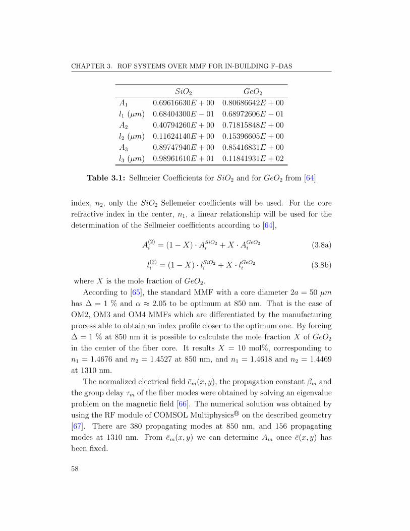
CHAPTER 3. ROF SYSTEMS OVER MMF FOR IN-BUILDING F–DAS
SiO2 GeO2
A1 0.69616630E + 00 0.80686642E + 00
l1 (µm) 0.68404300E − 01 0.68972606E − 01
A2 0.40794260E + 00 0.71815848E + 00
l2 (µm) 0.11624140E + 00 0.15396605E + 00
A3 0.89747940E + 00 0.85416831E + 00
l3 (µm) 0.98961610E + 01 0.11841931E + 02
Table 3.1: Sellmeier Coefficients for SiO2 and for GeO2 from [64]
index, n2, only the SiO2 Sellemeier coefficients will be used. For the core
refractive index in the center, n1, a linear relationship will be used for the
determination of the Sellmeier coefficients according to [64],
A(2)i = (1−X) · ASiO2
i +X · AGeO2i (3.8a)
l(2)i = (1−X) · lSiO2
i +X · lGeO2i (3.8b)
where X is the mole fraction of GeO2.
According to [65], the standard MMF with a core diameter 2a = 50 µm
has ∆ = 1 % and α ≈ 2.05 to be optimum at 850 nm. That is the case of
OM2, OM3 and OM4 MMFs which are differentiated by the manufacturing
process able to obtain an index profile closer to the optimum one. By forcing
∆ = 1 % at 850 nm it is possible to calculate the mole fraction X of GeO2
in the center of the fiber core. It results X = 10 mol%, corresponding to
n1 = 1.4676 and n2 = 1.4527 at 850 nm, and n1 = 1.4618 and n2 = 1.4469
at 1310 nm.
The normalized electrical field em(x, y), the propagation constant βm and
the group delay τm of the fiber modes were obtained by solving an eigenvalue
problem on the magnetic field [66]. The numerical solution was obtained by
using the RF module of COMSOL Multiphysics R© on the described geometry
[67]. There are 380 propagating modes at 850 nm, and 156 propagating
modes at 1310 nm. From em(x, y) we can determine Am once e(x, y) has
been fixed.
58
3.1. DEVELOPED THEORETICAL MODEL
In the case of an input electrical field coming from a single mode fiber,
e(x, y) was determined through the model described above assuming 2a =
9 µm, step-index profile (α→∞ in (3.6)), and X = 6.3 mol% [68]. Naming
eSMF (x, y) the normalized electrical field of the SMF centered with respect
to the SMF axis, in the case of central launch it is e(x, y) = eSMF (x, y), while
in the case of offset launch it is e(x, y) = eSMF (x − xoffset, y) where xoffsetis the misalignment between SMF and MMF.
Fig. 3.1 shows the values of A2m at 1310 nm in two cases: central launch
from a SMF in Fig. 3.1(a), and offset launch performed with xoffset = 12 µm
in Fig. 3.1(b). Note that central launch excites few modes, all exhibiting
a low mode number, m, (lower order modes), while offset launch excites a
larger number of modes, many of which are modes with a high mode number,
m, (higher order modes).
The reason to use offset launch is that, since in practice a perfect central
launch is not feasible and can be corrupted by modal coupling, offset launch
can guarantee a more stable situation compared to central launch. Moreover,
Raddatz et al. stated that this technique can enhance the bandwidth of
multimode fiber links [69, 70]. Anyway, this is not a general rule. Central
and offset launch performance depends on the MMF and other restricted
launch techniques can outperform central or offset launches [71, 72].
As mentioned above, with the MMF characterization performed with
COMSOL Multiphysics R© it was possible also to determine the propagation
constant βm and the group delay τm of every mode. In Fig. 3.2 typical values
of βm (a) and τm (b) are presented for a graded-index MMF at 1310 nm. Note
that βm in Fig. 3.2(a) has a stair-shape which allows to distinguish between
groups of modes with similar propagation constants. The group delays τm in
Fig. 3.2(b) are instead not exactly aligned on a stair-shape. Anyhow, I do not
assemble in this model the modes into groups, but I use the complete set of
modes, each one taken separately from the others. Furthermore, chromatic
or third-order dispersions of the modes are not considered since this model
is applied to short-range MMF link. However, analytical models taking into
account chromatic and third-order dispersions have been reported [73, 74].
Starting from (3.4) the electrical field after propagation in a MMF of
59

CHAPTER 3. ROF SYSTEMS OVER MMF FOR IN-BUILDING F–DAS
0 20 40 60 80 100 120 140 1560
0.1
0.2
0.3
0.4
0.5
0.6
Mode number m
Wei
gth
co
effi
cien
t A
m2
(a) Central launch
20 40 60 80 100 120 140 1560
0.02
0.04
0.06
0.08
0.1
Mode number m
Wei
gth
co
effi
cien
t A
m2
(b) Offset launch
Figure 3.1: Example of typical values of A2m in the case of central launch
(a) and offset launch with a displacement of 12 µm (b)
60

3.1. DEVELOPED THEORETICAL MODEL
1 20 40 60 80 100 120 140 156 6.94
6.95
6.96
6.97
6.98
6.99
7
7.01
7.02x 10
6
Mode number m
β m (
m−1
)
(a)
1 20 40 60 80 100 120 140 1564.9255
4.926
4.9265
4.927
4.9275x 10
−9
Mode number m
τ m (
s/m
)
(b)
Figure 3.2: Example of typical values of βm (a) and τm (b) for a graded-
index MMF at 1310 nm
61

CHAPTER 3. ROF SYSTEMS OVER MMF FOR IN-BUILDING F–DAS
length z becomes then,
Eout(t, z) = E0
NM∑m=1
Am · em(x, y) ·√
1 + y(t− τmz) ·
· exp [2πf0t− βmz + φm(t, z) + ψ(t− τmz)] (3.9)
The quantity φm(t) is a slow phase variation with respect to the theo-
retical phase shift, βmz, of the optical carrier [75]. This phase variation is
induced by fluctuations of environmental physical quantities, such as the am-
bient temperature or mechanical stress. The presence of this random phase
variation is the cause of modal noise. From a statistical point of view it is
possible to assume φm(t) of different modes uniformly distributed between
−π and +π and uncorrelated as done in [75]. This assumption does not de-
scribe any physical relationship between phase variations of different modes.
Indeed, the random phase variations described by φm(t) are related to the
changes of the refractive index profile, i.e. value and/or shape, caused by
temperature or stress variation. A thermo-optic coefficient around 10−5 /K
and a pressure-optic coefficient around 10−5 /106Nm−2 have been reported
for fused silica [76, 77]. Consequently, I assume that the effective index of
refraction of every mode changes with temperature or pressure. Then, I
define,
φm(t, z) =
(βm −
2π
λ0
neff,m(t)
)z (3.10)
where neff,m(t) is the effective index of refraction of the mth mode (n2 <
neff,m < n1) [57].
Since neff,m is related to the refractive indexes n1 and n2, it is reason-
able to consider also its time variations related to the time variations of the
same indexes. But, neff,m referred to different modes will experience a dif-
ferent strength of slow variations. As a first approximation I consider φm(t)
dependence from an external temperature variations ∆T (t) as,
φm(t, z) = cm ·∆T (t) + φ0,m (3.11)
where cm is a coefficient which takes into account the thermo-optic effects
and φ0,m is a random phase due to possible random imperfections of the fiber.
62

3.1. DEVELOPED THEORETICAL MODEL
The initial phase φ0,m can be chosen random between −π and +π, while
cm can be chosen randomly between a minimum value and a maximum value
with the same sign. These minimum and maximum values increase with
fiber length, z, and can be simply estimated to fit experimental data since
there is no simple direct relationship between refractive indexes and effective
refractive indexes variations. With this model φm(t) is still uniformly dis-
tributed between −π and +π, but phases related to different modes are no
more uncorrelated. Considering two phase variations φm and φm related to
mode m and n it is,
Cov (φm(t), φn(t)) = E [cmcn] · 〈[∆T (t)]2〉+ E [φ0,mφ0,n] (3.12)
where Cov (., .) stands for statistical covariance, E [.] for statistical averag-
ing, and 〈.〉 for time averaging. To obtain this result I took the hypothesis
〈∆T (t)〉 = 0 which comes from the definition of temperature variation.
The result in (3.12) demonstrates that even if the statistical couples cm,
cn and φ0,m, φ0,n are uncorrelated the covariance of φm and φn is not zero
since E [cmcn] is always a positive number. This is due to the hypothesis
of assuming cm to be positive or negative for all modes. This assumption
comes from the physical consideration that at a certain wavelength the index
of refraction always decreases or increases for a positive temperature variation
∆T .
3.1.3 Receiver model
After the propagation in one span of MMF, the electrical field is detected
by a photodiode. With respect to the SMF case of (2.28), it is crucial to
consider the finite detecting area of the photodiode. Indeed, if in the SMF
this means just a loss of optical power, in this case it also represents different
attenuations for the MMF modes, and different mutual interference.
63
CHAPTER 3. ROF SYSTEMS OVER MMF FOR IN-BUILDING F–DAS
The received electrical current generated by the photodiode is,
iout(t, z) = R ·∫SPD
∣∣Eout(t, z)∣∣22Z
dS = I0
NM∑m=1
A2mbmm (1 + y(t− τmz)) +
+2I0 · <
NM−1∑m=1
NM∑n=m+1
AmAnbmn ·√
1 + y(t− τmz)·
·√
1 + y(t− τnz) · exp [ψ(t− τmz)− ψ(t− τnz)] ·· exp [(φm(t, z)− φn(t, z))− (βm − βn) z] (3.13)
where I0 = RE20/2Z is the maximum possible direct current (DC) compo-
nent, <. stands for real part, and
bmn =
∫SPD
em (x, y) • e∗n (x, y) dS (3.14)
Note that bmn given by (3.14) is the scalar product between the normal-
ized electrical fields of MMF modes of numbers m and n computed over
the detecting area of the photodiode, SPD. Due to mode orthogonality, this
quantity should ideally be equal to one for m = n while it should be equal to
zero for m 6= n. However, because of the finite detecting area of the photodi-
ode neither condition is met. This non-ideal behavior is another factor which
influences modal noise. Fig. 3.3 shows typical values of bmm and bmn. In this
example I assumed that the photodiode surface was a square, with width 25
µm, misaligned of 2 µm with respect to the central axis of the MMF. From
Fig. 3.3(a) it can be observed that bmm values are mostly between 0.6 and 1
and tend to decrease for increasing m. This is due to the lower confinement
of higher order modes in the core of the MMF. Fig. 3.3(b) shows |bmn| for
n = 20. bm20 values are mainly between 1E − 4 and 1E − 1. Similar results
can be presented for different values of n.
The phase differences present in the second summation in (3.13) need to
be calculated,
ψ(t− τmz)− ψ(t− τnz) = − [xmn,1 cos (2πfc,1 (t− τmn − ν1)) +
+ xmn,2 cos (2πfc,2 (t− τmn − ν2))] (3.15)
64

3.1. DEVELOPED THEORETICAL MODEL
1 20 40 60 80 100 120 140 1560.4
0.5
0.6
0.7
0.8
0.9
1
Mode number m
bm
m
(a)
1 20 40 60 80 100 120 140 1561E−6
1E−5
1E−4
1E−3
1E−2
1E−1
1E 0
Mode number m
|bm
20|
(b)
Figure 3.3: Example of typical values of bmm (a) and bm20 (b) assuming the
photodiode surface as a square with side 25 µm and a misalign-
ment of 2 µm with respect to the central axis of the MMF
65

CHAPTER 3. ROF SYSTEMS OVER MMF FOR IN-BUILDING F–DAS
where
xmn,i = 4πKfIRF∆τmnsin (2πfc,i∆τmn)
2πfc,i∆τmnfor i = 1, 2 (3.16a)
∆τmn =τm − τn
2z (3.16b)
τmn =τm + τn
2z (3.16c)
The quantity xmn,i in (3.16a) will be shown to be an important parameter
which influences modal noise strength. It increases with the transmitter chirp
factor, Kf , and with the amplitude current, IRF . For the couples of modes
with |2πfc,i∆τmn| < π/2, xmn,i also increases with fiber length z. This is the
case of most of the couples of modes in short-range MMF link employing RF
frequencies below 2–3 GHz.
The other part of the phase in (3.13) can be collected in,
∆ϕmn(t) = (φm(t, z)− φn(t, z))− (βm − βn) z (3.17)
Using (3.11) ∆ϕmn can be written in a form similar to φm,
∆ϕmn(t) = cmn ·∆T (t) + ∆ϕ0,mn (3.18)
where cmn = cm− cn and ∆ϕ0,mn = (φ0,m − φ0,n)− (βm − βn) z. Similarly to
φ0,m or φ0,n, ∆ϕ0,mn can be chosen randomly between −π and +π. On the
other hand, contrary to cm or cn, cmn referred to different couples of modes
can have a different sign. This leads to take E [cmn] = 0. Consequently,
Cov (∆ϕmn(t),∆ϕkl(t)) referred to different mode couples (m,n) and (k, l)
can be zero if cmn, ckl, ∆ϕmn(t) and ∆ϕkl(t) are uncorrelated.
Using (3.15) and (3.17), (3.13) becomes,
iout(t, z) = I0
NM∑m=1
A2mbmm (1 + y(t− τmz)) + 2I0
NM−1∑m=1
NM∑n=m+1
AmAnbmn ·
·√
1 + y(t− τmz) + y(t− τnz) + y(t− τmz) · y(t− τnz) ·· [cos (∆ϕmn(t)) cos (xmn,1 cos (2πfc,1 (t− τmn − ν1)) +
+ xmn,2 cos (2πfc,2 (t− τmn − ν2))) +
+ sin (∆ϕmn(t)) sin (xmn,1 cos (2πfc,1 (t− τmn − ν1)) +
+ xmn,2 cos (2πfc,2 (t− τmn − ν2)))] (3.19)
66

3.1. DEVELOPED THEORETICAL MODEL
To determine the received current at each frequency all terms containing
the time variable, t, in (3.19) were expanded with analytical series:
• the square root by using the Maclaurin series [59]:
√1 + x =
∞∑k=0
(−1)k (2k)!
(1− 2k) (k!)2 (4k)xk (3.20)
where x is substitued by the content of the square root except from 1.
• the cos (xmn,1...+ xmn,1...) and sin (xmn,1...+ xmn,1...) by using the Jacobi-
Anger expansion [59]:
ejx cos θ = J0(x) + 2∞∑k=1
jkJk(x) cos(kθ) (3.21)
where Jk is a Bessel function of the kth order [59].
Due to the initial assumption to consider laser non-linearities up to the
third-order (see (3.2)), only power of mI up to the third order should be
taken into account. This means that the expansions in (3.20) and (3.21)
should be considered for k ≤ 3.
After a lengthy calculations the current can be determined at the following
frequency components: DC, fc,1, fc,2, 2fc,1, 2fc,2, fc,1+fc,2, 3fc,1, 3fc,2, 2fc,1−fc,2, and 2fc,2 − fc,1. The generic component at frequency f can be written
as,
iout,f (t, z) =(Ac,f + Bc,f (t)
)cos(2πft
)+(As,f + Bs,f (t)
)sin(2πft
)(3.22)
where
Ac,f = I0 · afNM∑m=1
A2mbmm cos
(2πfτmz
)(3.23a)
As,f = I0 · afNM∑m=1
A2mbmm sin
(2πfτmz
)(3.23b)
Bc,f (t) = 2I0
NM−1∑m=1
NM∑n=m+1
AmAnbmnDmn,f ,c(t) (3.23c)
67

CHAPTER 3. ROF SYSTEMS OVER MMF FOR IN-BUILDING F–DAS
Bs,f (t) = 2I0
NM−1∑m=1
NM∑n=m+1
AmAnbmnDmn,f ,s(t) (3.23d)
Dmn,f ,c(t) = Cmn,f ,C,c cos (∆ϕmn(t)) + Cmn,f ,S,c sin (∆ϕmn(t)) (3.23e)
Dmn,f ,s(t) = Cmn,f ,C,s cos (∆ϕmn(t)) + Cmn,f ,S,s sin (∆ϕmn(t)) (3.23f)
The value of af in (3.23a) and (3.23b) comes from (3.2). In particular it
is,
afc,1 = afc,2 = mI (3.24a)
a2fc,1 = a2fc,2 =1
2a2m
2I (3.24b)
a2fc,1−fc,2 = a2fc,2−fc,1 =3
4a3m
3I (3.24c)
The expressions of the terms Cmn,f ,C,c and Cmn,f ,S,c in (3.23e) and Cmn,f ,C,sand Cmn,f ,S,s in (3.23f) are reported in Tab. 3.2 for the component at DC and
at 2fc,1, in Tab. 3.3 for the component at fc,1, and in Tab. 3.4 for the compo-
nent at 2fc,2 − fc,1. The expressions referred to other frequency components
are not included in this thesis.
With all the terms in (3.22), the amplitude Iout,f of the component at
frequency f can be determined,
Iout,f (t) =
√(Ac,f + Bc,f (t)
)2+(As,f + Bs,f (t)
)2(3.25)
From (3.25) it is possible to observe that the amplitude of the current
at frequency f is ruled by non-fluctuating terms (Ac,f and As,f ) and time-
fluctuating terms (Bc,f (t) and Bs,f (t)). Indeed, these last terms depend from
the difference of phases ∆ϕmn(t) and represent the modal noise contribution.
The characterization of the statistical distribution of Iout,f (t) is complex
and in general possible only numerically. For this reason, I will only deter-
mine analytically the mean value of the received power at frequency f and
the standard deviation for the components at DC and fc,1. Other statistical
quantities used in this work are determined numerically.
68

3.1. DEVELOPED THEORETICAL MODEL
Tab
le3.2
:E
xpre
ssio
nofCmn,f,C,c
,Cmn,f,S,c
,Cmn,f,C,s
andCmn,f,S,s
for
DC
and
2fc,
1
DC
Cmn,DC,C,c
=J
0(x
mn,1
)J0(x
mn,2
)
1+m
2 I 8[c
os(2π
2fc,
1∆τ m
n)
+co
s(2π
2fc,
2∆τ m
n)−
2]
Cmn,DC,S,c
=mI
[J0(x
mn,1
)J1(x
mn,2
)co
s(2πf c,2
∆τ m
n)
cos
(2πf c,1ν 1
)+
J0(x
mn,2
)J1(x
mn,1
)co
s(2πf c,1
∆τ m
n)
cos
(2πf c,2ν 2
)]
Cmn,DC,C,s
=0
Cmn,DC,S,s
=0
2fc,
1
Cmn,2fc,1,C,c
=m
2 I 8J
0(x
mn,1
)J0(x
mn,2
)[(
4a2−
1)co
s(2π
2fc,
1∆τ m
n)
+1]
cos
(2π
(2f c,1
)τmn)−
2J0(x
mn,2
)J2(x
mn,1
)cos
(2π
2fc,
1(τmn
+ν 1
))
Cmn,2fc,1,S,c
=mIJ
0(x
mn,2
)J1(x
mn,1
)co
s(2πf c,1
∆τ m
n)
cos
(2π
(2f c,1τ m
n+f c,1ν 1
))
Cmn,2fc,1,C,s
(Cmn,2fc,1,S,s
)id
enti
cal
toCmn,2fc,1,C,c
(Cmn,2fc,1,S,c
)w
ith
cos
subst
itute
dw
ith
sin
69

CHAPTER 3. ROF SYSTEMS OVER MMF FOR IN-BUILDING F–DAS
Table
3.3
:E
xpression
ofCmn,fc,1,C,c ,Cmn,c,1,S,c ,Cmn,fc,1,C,s
andCmn,fc,1,S,s
fc,1
Cmn,fc,1,C,c
=J
0 (xmn,1 )J
0 (xmn,2 )
mI
cos(2π
fc,1 ∆
τmn )
+m
3I
32(4a
2 −1)
[(4cos
(2π2f
c,2 ∆τmn )−
5)·
cos(2π
fc,1 ∆
τmn )
+cos
(2π3f
c,1 ∆τmn )]
cos(2π
fc,1 τ
mn )−
mI J
0 (xmn,2 )J
2 (xmn,1 )
cos(2π
fc,1 ∆
τmn )
cos(2π
fc,1 (τ
mn
+2ν
1 ))−2m
I J1 (x
mn,1 )J
1 (xmn,2 )
cos(2π
fc,2 ∆
τmn )
cos(2π
fc2 ν
2 )cos
(2πfc,1 (τ
mn
+ν
1 ))
Cmn,fc,1,S,c
=J
0 (xmn,2 )J
1 (xmn,1 )
2+m
2I
8[4
cos(2π
2fc,2 ∆
τmn )−
3+
(4a2 −
1)cos
(2π2f
c,1 ∆τmn )]
·
cos(2π
fc,1 (τ
mn
+ν
1 ))+J
0 (xmn,1 )J
1 (xmn,2 ) m
2I
4[2a
2cos
(2π(fc,2 −
fc,1 )∆
τmn )−
sin(2π
fc,1 ∆
τmn )
sin(2π
fc,2 ∆
τmn )]cos
(2π(fc,1 τ
mn
+fc,2 ν
2 ))+
[2a2
cos(2π
(fc,1
+fc,2 )∆
τmn )−
sin(2π
fc,1 ∆
τmn )
sin(2π
fc,2 ∆
τmn )]cos
(2π(fc,1 τ
mn−fc,2 ν
2 ))Cmn,fc,1,C,s
(Cmn,fc,1,S,s )
iden
ticaltoCmn,fc,1,C,c
(Cmn,fc,1,S,c )
with
cossu
bstitu
tedw
ithsin
70

3.1. DEVELOPED THEORETICAL MODEL
Tab
le3.4
:E
xpre
ssio
nofCmn,2fc,2−fc,1,C,c
,Cmn,2fc,2−fc,1,S,c
,Cmn,2fc,2−fc,1,C,s
andCmn,2fc,2−fc,1,S,s
2fc,
2−f c,1
Cmn,2fc,2−fc,1,C,c
=m
3 I
32J
0(x
mn,1
)J0(x
mn,2
)[3
(8a
3−
4a2
+1)
cos
(2π
(2f c,2−f c,1
)∆τ m
n)
+(4a
2−
1)·
(cos
(2π
(2f c,2
+f c,1
)∆τ m
n)
+2
cos
(2πf c,1
∆τ m
n))
]co
s(2π
(2f c,2−f c,1
)τmn)−
mIJ
0(x
mn,1
)J2(x
mn,2
)co
s(2πf c,1
∆τ m
n)
cos
(2π
((2f
c,2−f c,1
)τmn
+2f
c,2ν 2
))−
J1(x
mn,1
)J1(x
mn,2
)co
s(2πf c,2
∆τ m
n)
cos
(2π
((2f
c,2−f c,1
)τmn
+f c,2ν 2−f c,1ν 1
))
Cmn,2fc,2−fc,1,S,c
=m
2 I 82J
0(x
mn,1
)J1(x
mn,2
)[(
4a2−
1)co
s(2π
(fc,
2−f c,1
)∆τ m
n)
+co
s(2π
(fc,
2+f c,1
)∆τ m
n)]·
cos
(2π
((2f
c,2−f c,1
)τmn
+f c,2ν 2
))+J
0(x
mnm,2
)J1(x
mn,1
)[(
4a2−
1)co
s(2π
2fc,
2∆τ m
n)
+1]·
cos
(2π
((2f
c,2−f c,1
)τmn−f c,1ν 1
))−
2J1(x
mn,1
)J2(x
mn,2
)cos
(2π
((2f
c,2−f c,1
)τmn
+2f
c,2ν 2−f c,1ν 1
))
Cmn,2fc,2−fc,1,C,s
(Cmn,2fc,2−fc,1,S,s
)id
enti
cal
toCmn,2fc,2−fc,1,C,c
(Cmn,2fc,2−fc,1,S,c
)w
ith
cos
subst
itute
dw
ith
sin
71

CHAPTER 3. ROF SYSTEMS OVER MMF FOR IN-BUILDING F–DAS
The received power at frequencies f is,
Pout,f (t) =RL
2I2out,f (t) =
RL
2
[(Ac,f + Bc,f (t)
)2+(As,f + Bs,f (t)
)2]
(3.26)
where RL is the load resistance (50Ω).
The mean electrical power at frequencies f is,
〈Pout,f (t)〉 =RL
2
(A2c,f + A2
s,f + 〈B2c,f (t)〉+ 〈B2
s,f (t)〉+
+ 2Ac,f〈Bc,f (t)〉+ 2As,f〈Bs,f (t)〉)
(3.27)
To determine 〈Pout,f (t)〉 it is necessary to calculate the mean and the
mean square value of Bc,f (t) and Bs,f (t). For the mean value it is,
〈Bc,f (t)〉 = 2I0
NM−1∑m=1
NM∑n=m+1
AmAnbmn〈Dmn,f ,c(t)〉 = 0 (3.28)
where I used the property of the mean value of Dmn,f ,c(t) to be equal to zero
since ∆ϕmn(t), as φm, uniformly distributed between −π and +π.
The mean square value is,
〈B2c,f (t)〉 = 4I2
0
NM−1∑m=1
NM∑n=m+1
NM−1∑k=1
NM∑l=m+1
AmAnAkAlbmnbkl〈Dmn,f ,c(t)Dkl,f ,c(t)〉
(3.29)
In (3.29) we need to determine 〈Dmn,f ,c(t)Dkl,f ,c(t)〉,
〈Dmn,f ,c(t)Dkl,f ,c(t)〉 = Cmn,f ,C,cCkl,f ,C,c〈cos (∆ϕmn(t)) cos (∆ϕkl(t))〉++ Cmn,f ,C,cCkl,f ,S,c〈cos (∆ϕmn(t)) sin (∆ϕkl(t))〉++ Cmn,f ,S,cCkl,f ,C,c〈sin (∆ϕmn(t)) cos (∆ϕkl(t))〉++ Cmn,f ,S,cCkl,f ,S,c〈sin (∆ϕmn(t)) sin (∆ϕkl(t))〉
(3.30)
To simplify (3.30) I use the assumption described above that ∆ϕmn and
∆ϕkl are uncorrelated. This leads to,
〈cos (∆ϕmn(t)) cos (∆ϕkl(t))〉 =1
2(δmkδnl + δmlδnk) (3.31a)
72

3.1. DEVELOPED THEORETICAL MODEL
〈sin (∆ϕmn(t)) sin (∆ϕkl(t))〉 =1
2(δmkδnl − δmlδnk) (3.31b)
〈cos (∆ϕmn(t)) sin (∆ϕkl(t))〉 = 0 (3.31c)
where δmk is the Kronecker delta function.
Substituting (3.31a), (3.31b) and (3.31c) in (3.30) it is,
〈Dmn,f ,c(t)Dkl,f ,c(t)〉 =C2mn,f ,C,c
+ C2mn,f ,S,c
2· (δmkδnl + δmlδnk) (3.32)
Substituting (3.32) in (3.29) we have,
〈B2c,f (t)〉 = 2I2
0
NM−1∑m=1
NM∑n=m+1
A2mA
2nb
2mn ·
[C2mn,f ,C,c + C2
mn,f ,S,c
](3.33)
and similarly for B2s,f
(t).
Substituting (3.23a), (3.23b), (3.28) and (3.33) in (3.27) the mean value
can be determined as,
〈Pout,f (t)〉 =RL
2I2
0
a2f
[NM∑m=1
A4mb
2mm + 2
NM−1∑m=1
NM∑n=1
A2mA
2nbmmbnn·
· cos(2πf2∆τmn
)]+ 2
NM−1∑m=1
NM∑n=1
A2mA
2nb
2mn·
·(C2mn,f ,C,c + C2
mn,f ,S,c + C2mn,f ,C,s + C2
mn,f ,S,s
)(3.34)
The variance of the electrical power at frequencies f is,
Var(Pout,f (t)
)=Var
(B2c,f (t) + B2
s,f (t))
+ 4 · Var(Ac,fBc,f (t) + As,f ·
·Bs,f (t))
+ 4 · Cov(B2c,f (t) + B2
s,f (t),As,fBs,f + As,fBs,f
)(3.35)
To determine the variance in (3.35) it is necessary to calculate the mean
value of powers of Bc,f (t) and Bs,f (t) up to the fourth order, which involves
calculation even longer than the one reported for 〈Pout,f (t)〉. For this reason
73
CHAPTER 3. ROF SYSTEMS OVER MMF FOR IN-BUILDING F–DAS
I report analytical results just for the cases where it is B2c,f
(t) + B2s,f
(t) A2c,f
+ A2s,f
. This leads to assume,
Pout,f (t) ≈RL
2
(A2c,f + A2
s,f + 2Ac,fBc,f (t) + 2As,fBs,f (t))
(3.36)
Utilizing (3.36) the mean value and the variance of Pout,f (t) simplify to,
〈Pout,f (t)〉 ≈RL
2
(A2c,f + A2
s,f
)(3.37a)
Var(Pout,f (t)
)≈ R2
L · Var(Ac,fBc,f (t) + As,fBs,f (t)
)=
= R2L
(A2c,f〈Bc,f (t)
2〉+ A2s,f〈Bs,f (t)
2〉+
+ 2Ac,fAs,f〈Bc,f (t) ·Bs,f (t)〉)
(3.37b)
All the terms in (3.37b) have been already determined apart from 〈Bc,f (t)·Bs,f (t)〉. Following the same approach used to obtain 〈Bc,f (t)
2〉 in (3.33), it
is,
〈Bc,f (t)Bs,f (t)〉 =2I20
NM−1∑m=1
NM∑n=m+1
A2mA
2nb
2mn·
·[Cmn,f ,C,cCmn,f ,C,s + Cmn,f ,S,cCmn,f ,S,s
](3.38)
Substituting (3.33) and (3.38) in (3.37b), we have finally,
Var(Pout,f (t)
)≈R2
LI20
NM−1∑m=1
NM∑n=m+1
A2mA
2nb
2mn·
·[(Ac,fCmn,f ,C,c + As,fCmn,f ,C,s
)2+
+(Ac,fCmn,f ,S,c + As,fCmn,f ,S,s
)2]
(3.39)
The formula in (3.39) is a good approximation of the variance of the
received component at frequency f if the non-fluctuating term A2c,f
+ A2s,f
prevails on the fluctuating term B2c,f
(t) +B2s,f
(t). This is the case for the DC
component and the component at fc,1 if not close to a minimum of the MMF
transfer function. For the component at other frequencies this approximation
is not valid since the received non-fluctuating term has typically very low
values.
74

3.1. DEVELOPED THEORETICAL MODEL
3.1.4 Extension to multi-wavelength sources
The model presented in the previous subsections refers to a single-wave-
length laser, such as a DFB LD. However, in MMF systems also multi-
wavelength lasers, such as FP LDs, are currently employed. For this reason,
it is meaningful to extend the previous model to multi-wavelength sources.
The starting point is the electrical field EMW (t) emitted from a multi-
wavelength source,
EMW (t) =
NW∑k=1
E(k)0 · e(k)(x, y) ·
√1 + y(k)(t) ·exp
[2πfkt+ ψ(k)(t)
](3.40)
Referring to the generic wavelength k, fk is the optical frequency, and
all the other quantities have the same meaning of (3.1) with the superscript
(k) which applies to all the implicit quantities in (3.40) which depend on the
wavelength.
Since the different wavelengths can be considered completely uncorre-
lated, the electrical field can be written as,
EMW (t) =
NW∑k=1
E(k)in (t) (3.41)
where E(k)in (t) is the normalized electrical field produced by the kth wave-
length.
Since the MMF is a linear medium, also the output electrical field is
a superposition of the electrical field generated by the propagation of the
electrical field of each wavelength giving,
Eout,MW (t, z) =
NW∑k=1
E(k)out(t) (3.42)
where E(k)out(t) is the normalized electrical field produced by the kth wave-
length. Its mathematical expression is the same in (3.9) with the superscript
(k) applied to all the quantities which depend on the wavelength.
75

CHAPTER 3. ROF SYSTEMS OVER MMF FOR IN-BUILDING F–DAS
The electrical received current is,
iout,MW (t, z) =R
∫SPD
∣∣Eout,MW (t, z)∣∣2
2ZdS =
R
2Z
[NW∑k=1
∫SPD
(E
(k)out(t)
)2
dS+
+2
NW−1∑k=1
NW∑l=k+1
∫SPD
E(k)out(t)E
(l)out(t)dS
](3.43)
Since in a multi-wavelength source the distance between two adjacent
wavelengths is of the order of hundreds of GHz, the cross-product between
two electrical fields referred to different wavelengths cannot be detected by
a common photodiode. Hence, (3.43) simplifies to,
iout,MW (t, z) =
NW∑k=1
R
2Z
∫SPD
(E
(k)out(t)
)2
dS =
NW∑k=1
i(k)out(t, z) (3.44)
Equation (3.44) states that the received current from a multi-wavelength
source is the superposition of the received current of each wavelength taken
separately. Since the component of the current at frequency f of each wave-
length can be written as (3.22), the overall received current can also be
written in a similar way,
iout,MW,f (t, z) =(Ac,MW,f + Bc,MW,f (t)
)cos(2πft
)+
+(As,MW,f + Bs,MW,f (t)
)sin(2πft
)(3.45)
where
Ac,MW,f =
NW∑k=1
I(k)0 · a
(k)
f
NM∑m=1
(A(k)m
)2b(k)mm cos
(2πfτ (k)
m z)
(3.46a)
As,MW,f =
NW∑k=1
I(k)0 · a
(k)
f
NM∑m=1
(A(k)m
)2b(k)mm sin
(2πfτ (k)
m z)
(3.46b)
Bc,MW,f (t) = 2
NW∑k=1
I(k)0 ·
NM−1∑m=1
NM∑n=m+1
A(k)m A(k)
n b(k)mnD
(k)
mn,f ,c(t) (3.46c)
76
3.1. DEVELOPED THEORETICAL MODEL
Bs,MW,f (t) = 2
NW∑k=1
I(k)0 ·
NM−1∑m=1
NM∑n=m+1
A(k)m A(k)
n b(k)mnD
(k)
mn,f ,s(t) (3.46d)
D(k)
mn,MW,f ,c(t) = C
(k)
mn,f ,C,ccos(∆ϕ(k)
mn(t))
+ C(k)
mn,f ,S,csin(∆ϕ(k)
mn(t))
(3.46e)
D(k)
mn,MW,f ,s(t) = C
(k)
mn,f ,C,scos(∆ϕ(k)
mn(t))
+ C(k)
mn,f ,S,ssin(∆ϕ(k)
mn(t))
(3.46f)
The terms C(k)
mn,f ,C,c, C
(k)
mn,f ,S,c, C
(k)
mn,f ,C,s, and C
(k)
mn,f ,S,sin (3.46e) and
(3.46f) have the same expression of Cmn,f ,C,c, Cmn,f ,S,c, Cmn,f ,C,s, and Cmn,f ,S,sin (3.23e) and (3.23f) with the superscript (k) applied to all the quantities
which depend on the wavelength.
In this work, when applying this model I will take the simplification of
considering only the phase differences ∆ϕ(k)mn(t) as depending on the wave-
length , while I will take all the other quantities as wavelength independent.
This means to assume the laser modulation characteristics indicated by mI ,
a2, a3, Kf , ν1 and ν2 to be similar for all the wavelengths emitted by the
laser. Moreover, I will take all the quantities related to MMF launch and
propagation independent from the wavelength as well. This assumption is
supported by the consideration that all the presented results are reported
around 1310 nm where the material dispersion is minimum. This means
that the fiber index profile is almost constant for all the wavelength of the
source and consequently the quantities A(k)m , b
(k)mm, b
(k)mn, τ
(k)m can be considered
wavelength independent. With this assumptions it follows that:
Ac,MW,f = I tot0 · afNM∑m=1
A2mbmm cos
(2πfτmz
)= I tot0 ·Ac,SW,f (3.47a)
As,MW,f = I tot0 · afNM∑m=1
A2mbmm sin
(2πfτmz
)= I tot0 ·As,SW,f (3.47b)
Bc,MW,f (t) = 2
NM−1∑m=1
NM∑n=m+1
AmAnbmn
NW∑k=1
I(k)0 D
(k)
mn,f ,c(t) (3.47c)
Bs,MW,f (t) = 2
NM−1∑m=1
NM∑n=m+1
AmAnbmn
NW∑k=1
I(k)0 D
(k)
mn,f ,s(t) (3.47d)
77
CHAPTER 3. ROF SYSTEMS OVER MMF FOR IN-BUILDING F–DAS
D(k)
mn,MW,f ,c(t) = Cmn,f ,C,c cos
(∆ϕ(k)
mn(t))
+ Cmn,f ,S,c sin(∆ϕ(k)
mn(t))
(3.47e)
D(k)
mn,MW,f ,s(t) = Cmn,f ,C,s cos
(∆ϕ(k)
mn(t))
+ Cmn,f ,S,s sin(∆ϕ(k)
mn(t))
(3.47f)
where I tot0 =∑NW
k=1 I(k)0 is the maximum DC component received from the
multi-wavelength source.
Assuming as uncorrelated the phase differences ∆ϕ(k)mn(t) related to dif-
ferent wavelengths, it is possible to determine, as it has been done for (3.34),
the mean value of the received power at frequency f ,
〈Pout,MW,f (t)〉 =RL
2
(I tot0
)2 · a2f
[NM∑m=1
A4mb
2mm + 2
NM−1∑m=1
NM∑n=1
A2mA
2nbmmbnn·
· cos(2πf2∆τmn
)]+ 2
NW∑k=1
(I
(k)0
)2
·NM−1∑m=1
NM∑n=1
A2mA
2nb
2mn·
·(C2mn,f ,C,c + C2
mn,f ,S,c + C2mn,f ,C,s + C2
mn,f ,S,s
)(3.48)
The approximate expression for the mean value, 〈Pout,MW,f (t)〉, and for
the variance, Var(Pout,MW,f (t)
), in the case of small fluctuations are,
〈Pout,MW,f (t)〉 ≈RL
2
(I tot0
)2 ·(A2c,SW,f + A2
s,SW,f
)(3.49a)
Var(Pout,MW,f (t)
)≈R2
L
(I tot0
)2 ·NW∑k=1
(I
(k)0
)2
·NM−1∑m=1
NM∑n=m+1
A2mA
2nb
2mn·
·[(Ac,SW,fCmn,f ,C,c + As,SW,fCmn,f ,C,s
)2+
+(Ac,SW,fCmn,f ,S,c + As,SW,fCmn,f ,S,s
)2]
(3.49b)
The mean power, 〈Pout,MW,f (t)〉, and the variance, Var(Pout,MW,f (t)
),
given by (3.49a) and (3.49b), respectively, are identical to the expression
derived in (3.37a) and (3.39) for a single-wavelength source apart from the
current I0 substituted with I tot0 in (3.49a), which is not due to a modal noise
effect, and substituted with∑NW
k=1(I(k)0 )2 in (3.49b), which comes from modal
noise. This term represents the benefit on modal noise due to the use of a
78

3.2. EXPERIMENTAL AND THEORETICAL RESULTS
multi-wavelength source with respect to a single-wavelength source. Using
the Cauchy’s inequality [59] it is indeed possible to prove that,∑NWk=1
(I
(k)0
)2
(I tot0 )2 =
∑NWk=1
(I
(k)0
)2
(∑NWk=1 I
(k)0
)2 ≥1
NW
(3.50)
where the equality holds when I(k)0 is identical for all wavelengths.
This means that a maximum reduction of the impact on modal noise
of NW times on 〈Pout,MW,f〉 and Var(Pout,MW,f (t)
)is theoretically possible.
However, the number of wavelengths is not the only parameter which in-
fluences modal noise. A case by case study is therefore performed in the
experimental section.
3.2 Experimental and theoretical results
In this section experimental results regarding the impact of modal noise
on link gain, harmonic and intermodulation distortions will be presented and
explained with the aid of simulation results obtained by the application of
the model described in section 3.1.
3.2.1 Experimental setup
Fig. 3.4 shows the general setup used for the experimental activity on link
gain and harmonic and intermodulation distortions. An Anritsu MS4624B
three-port vector network analyzer (VNA) was used as RF source and re-
ceiver. In particular, two of the VNA ports were used as RF sources and
one as receiver. The two source ports emitted two RF tones at different
frequencies, fc,1 and fc,2. The two tones were multiplied together using a
RF coupler and frequencies higher than fc,1 and fc,2 were removed with a
low-pass filter. This filter prevented higher order harmonics of fc,1 and fc,2coming from the VNA to modulate the RoF TX. The filtered combination
of the two tones modulated a RoF TX, based on directly modulated DFB
or FP LD at 1310 nm. All the RoF TXs had a single-mode pig-tail. Hence,
79

CHAPTER 3. ROF SYSTEMS OVER MMF FOR IN-BUILDING F–DAS
RoF TX RoF RX
VNA
Σ
SMF MMF MMF
LaunchClimatic
Chamber
MMFLength z
CIN (fc,1)
CIN (fc,2)
C
HD2
IMD3
+ 0.30 V
Multimeter
Figure 3.4: Experimental setup for the characterization of a RoMMF link
it was possible to apply a restricted launch condition to the MMF. In par-
ticular, three types of launch were investigated: central launch, offset launch
and overfilled launch.
Several spans of OM2 MMF were employed obtaining a total length rang-
ing from 75 to 525 m. The MMF spans were inserted in a climatic chamber
and underwent a controlled temperature variation. In this way, they were
forced to experience typical environmental temperature changes in a much
shorter time giving stable results and a repeatable experimental condition.
The received optical power was detected by a RoF RX based on InGaAs PIN
photodiodes equipped with multi-mode pigtail. No electrical amplification
stage was used in this kind of measurements since the purpose was to de-
termine non-linear distortions induced by the optical part of the RoMMF
link. Apart from the received power at the different frequencies, measured
by the VNA, also the received DC component and the temperature of the
climatic chamber were monitored. The DC component was measured with
a HP 3478A digital multimeter connected to an output DC port of the RoF
RX, while the temperature was measured by a thermocouple placed in the
climatic chamber. All the measured quantities were collected by a computer.
The set of realized measurements were chosen to investigate the impact
80
3.2. EXPERIMENTAL AND THEORETICAL RESULTS
on modal noise of the following aspects of the optical part of the RoMMF
link:
• Launch condition
• Photodiode collecting area characteristics
• Laser modulation characteristics
The impact of these characteristics on modal noise will in general be de-
scribed in terms of statistical quantities, such as mean value and variance.
However, I also present the relationship between the time behavior of com-
ponents at different frequencies and the variation of temperature. This is the
first point I will deal with, because it allows to have a clearer physical insight
on the characteristics of modal noise, allowing to understand what is behind
the various statistical quantities that will be considered in the following.
3.2.2 Time behavior of received power
The simple way to describe the relationship between the time behavior of
different frequency components of the received signal is to assume that all the
received quantities vary in the same way with different peak-to-peak values.
Hence, the time fluctuations normalized on the respective mean value is in
this case the same. That was the reason to use the speckle contrast γ2 as
the modal noise parameter [78, 79]. The speckle contrast is the normalized
variance of the intensity distribution at the output of the MMF. In our case
we are not interested in the normalized variance of a single speckle but of
all the intensity distribution received by the finite area of the photodiode.
Thus, I define a quantity Γ2DC similar to the speckle contrast but referred to
all the power received by the photodiode, which is proportional to the DC
current,
Γ2DC =
Var(Iout,DC)
(〈Iout,DC〉)2(3.51)
where Iout,DC is the received DC current as in (3.25) with f = 0.
81
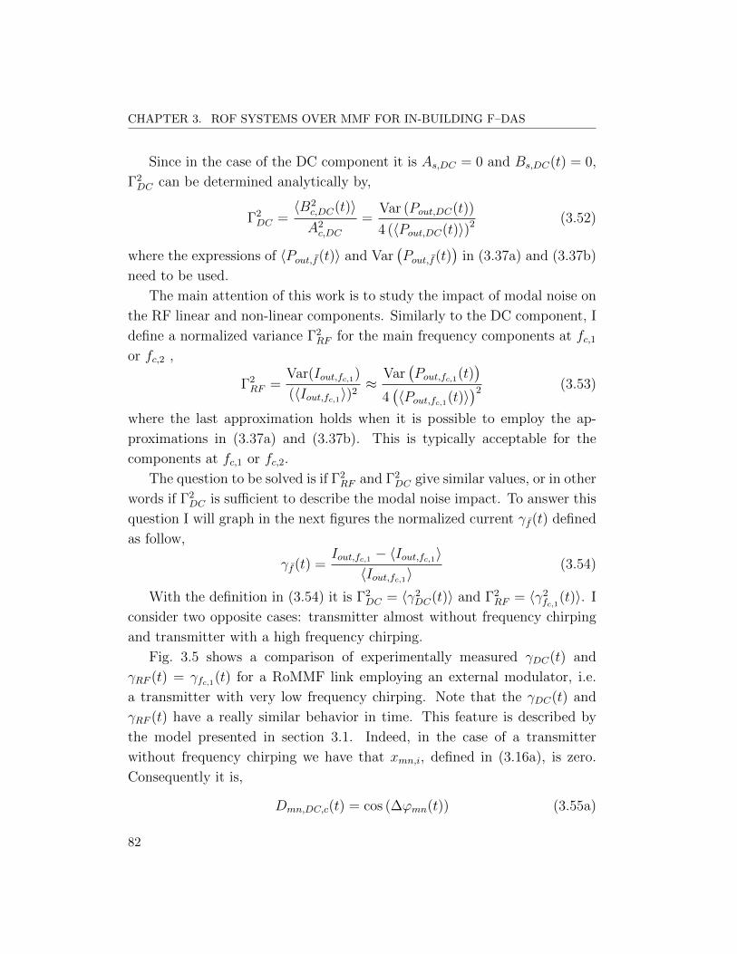
CHAPTER 3. ROF SYSTEMS OVER MMF FOR IN-BUILDING F–DAS
Since in the case of the DC component it is As,DC = 0 and Bs,DC(t) = 0,
Γ2DC can be determined analytically by,
Γ2DC =
〈B2c,DC(t)〉A2c,DC
=Var (Pout,DC(t))
4 (〈Pout,DC(t)〉)2 (3.52)
where the expressions of 〈Pout,f (t)〉 and Var(Pout,f (t)
)in (3.37a) and (3.37b)
need to be used.
The main attention of this work is to study the impact of modal noise on
the RF linear and non-linear components. Similarly to the DC component, I
define a normalized variance Γ2RF for the main frequency components at fc,1
or fc,2 ,
Γ2RF =
Var(Iout,fc,1)
(〈Iout,fc,1〉)2≈
Var(Pout,fc,1(t)
)4(〈Pout,fc,1(t)〉
)2 (3.53)
where the last approximation holds when it is possible to employ the ap-
proximations in (3.37a) and (3.37b). This is typically acceptable for the
components at fc,1 or fc,2.
The question to be solved is if Γ2RF and Γ2
DC give similar values, or in other
words if Γ2DC is sufficient to describe the modal noise impact. To answer this
question I will graph in the next figures the normalized current γf (t) defined
as follow,
γf (t) =Iout,fc,1 − 〈Iout,fc,1〉
〈Iout,fc,1〉(3.54)
With the definition in (3.54) it is Γ2DC = 〈γ2
DC(t)〉 and Γ2RF = 〈γ2
fc,1(t)〉. I
consider two opposite cases: transmitter almost without frequency chirping
and transmitter with a high frequency chirping.
Fig. 3.5 shows a comparison of experimentally measured γDC(t) and
γRF (t) = γfc,1(t) for a RoMMF link employing an external modulator, i.e.
a transmitter with very low frequency chirping. Note that the γDC(t) and
γRF (t) have a really similar behavior in time. This feature is described by
the model presented in section 3.1. Indeed, in the case of a transmitter
without frequency chirping we have that xmn,i, defined in (3.16a), is zero.
Consequently it is,
Dmn,DC,c(t) = cos (∆ϕmn(t)) (3.55a)
82
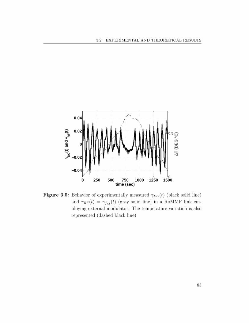
3.2. EXPERIMENTAL AND THEORETICAL RESULTS
0 250 500 750 1000 1250 1500
−0.04
−0.02
0
0.02
0.04
time (sec)
γ DC(t
) an
d γ R
F(t
)
0
0.5
∆T (
DE
G °
C)
Figure 3.5: Behavior of experimentally measured γDC(t) (black solid line)
and γRF (t) = γfc,1(t) (gray solid line) in a RoMMF link em-
ploying external modulator. The temperature variation is also
represented (dashed black line)
83

CHAPTER 3. ROF SYSTEMS OVER MMF FOR IN-BUILDING F–DAS
Dmn,fc,1,c(t) = mI cos (2πfc,1∆τmn) cos (2πfc,1τmn) cos (∆ϕmn(t)) (3.55b)
Dmn,fc,1,s(t) = mI cos (2πfc,1∆τmn) sin (2πfc,1τmn) cos (∆ϕmn(t)) (3.55c)
where I neglect all the terms which depends on powers of mI greater than
one.
From (3.55a), (3.55b), and (3.55c) it is clear that in the case of no trans-
mitter frequency chirping both Dmn,DC,c(t), Dmn,fc,1,c(t) and Dmn,fc,1,s(t) vary
with the same phase fluctuation, cos (∆ϕmn(t)), related to the temperature
variation ∆T (t). The received DC and RF current can be written as,
iout,DC(t, z) = I0
[NM∑m=1
A2mbmm + 2
NM−1∑m=1
NM∑n=m+1
AmAnbmn cos (∆ϕmn(t))
](3.56a)
iout,fc,1(t, z) =mII0
[NM∑m=1
A2mbmm cos (2πfc,1(t− τm)) + 2
NM−1∑m=1
NM∑n=m+1
AmAn·
·bmn cos (2πfc,1∆τmn) cos (∆ϕmn(t)) cos (2πfc,1(t− τmn))]
(3.56b)
To determine the relationship between the amplitude of iout,DC(t, z) and
of iout,fc,1(t, z) I take the simplification τm ≈ τn ≈ τmn, defined in (3.16a),
implying that ∆τmn, defined in (3.16c), is an infinitesimal quantity. In other
word I suppose to use a frequency fc,1 which is below the 3 dB low-pass
bandwidth. With this assumption the amplitude of the current iout,fc,1(t, z)
becomes,
iout,fc,1(t, z) ≈ mI · iout,DC(t, z) (3.57)
From (3.57) it is,
γRF (t) ≈ γDC(t) = 2
∑NM−1m=1
∑NMn=m+1AmAnbmn cos (∆ϕmn(t))∑NM
m=1A2mbmm
(3.58)
This explains why in Fig. 3.5 γDC(t) and γRF (t) present very similar time
behaviors. Consequently, it is Γ2DC = Γ2
RF and it is possible to show that the
same relationship is valid for different frequency components. Hence, in the
84
3.2. EXPERIMENTAL AND THEORETICAL RESULTS
0 500 1000 1500−0.1
−0.05
0
0.05
0.1
time (sec)
γ DC(t
) an
d γ R
F(t
)
0
0.5
1
∆T (
DE
G °
C)
Figure 3.6: Behavior of experimentally measured γDC(t) (black solid line)
and γRF (t) = γfc,1(t) (gray solid line) in a RoMMF link employ-
ing directly modulated DFB LD with high frequency chirping.
The temperature variation is also represented (dashed black
line)
case of a transmitter almost without frequency chirping the quantity Γ2DC ,
or speckle contrast, is sufficient to describe the statistical behavior of all the
received quantities.
Fig. 3.6 shows instead a comparison of experimentally measured γDC(t)
and γRF (t) = γfc,1(t) for a RoMMF link employing a RoF TX with a high
chirp parameter, Kf . There are two major differences with respect to Fig. 3.5.
First, the peak-to-peak value of γRF (t) is much greater that the one of γDC(t),
meaning that the impact of modal noise on the component at fc,1 is higher
than on the DC component. Secondly, the time behavior of the two quantities
is different. In particular, when one of the two is reaching a local maximum or
minimum the other is almost zero and is changing with a local high derivative.
This leads to presume that there is a kind of derivative relationship between
the two γ values.
This feature is described by the model presented in section 3.1. Indeed,
85

CHAPTER 3. ROF SYSTEMS OVER MMF FOR IN-BUILDING F–DAS
in the case of a transmitter with a nonzero frequency chirping, xmn,i, defined
in (3.16a), is not anymore zeros. It is then,
Dmn,DC,c(t) = J0(xmn,1)J0(xmn,2) cos (∆ϕmn(t)) (3.59a)
Dmn,fc,1,c(t) = [mIJ0(xmn,1)J0(xmn,2) cos (2πfc,1∆τmn) cos (∆ϕmn(t)) +
+2J0(xmn,2)J1(xmn,1) sin (∆ϕmn(t))] cos (2πfc,1τmn) (3.59b)
Dmn,fc,1,s(t) = [mIJ0(xmn,1)J0(xmn,2) cos (2πfc,1∆τmn) cos (∆ϕmn(t)) +
+2J0(xmn,2)J1(xmn,1) sin (∆ϕmn(t))] sin (2πfc,1τmn) (3.59c)
where I assumed for simplicity ν1 ≈ 0.
Comparing (3.55a) with (3.59a), there is no major difference apart from
a coefficient reduction, compared to 1, performed by J0(xmn,1)J0(xmn,2). In-
stead, comparing (3.59b) and (3.59c) with (3.55b) and (3.55c), we find now
a new addend multiplying sin (∆ϕmn(t)) in addition to the one multiplying
cos (∆ϕmn(t)). Assuming also in this case τm ≈ τn ≈ τmn, we have,
Iout,fc,1(t, z) ≈mI · iout,DC(t, z) + 4I0
NM−1∑m=1
NM∑n=m+1
AmAnbmn·
· J0(xmn,2)J1(xmn,1) sin (∆ϕmn(t)) (3.60)
It is confirmed from (3.60) that the amplitude of the component at fc,1can be written as in (3.57) with the addition of a fluctuating component
due to transmitter frequency chirping. Remembering the definition of xmn,iin (3.16a) and applying the approximation at the first order of the Bessel
functions J0(x) ≈ 1, J1(x) ≈ x/2 for low values of x, it is,
Iout,fc,1(t, z) ≈mI · iout,DC(t, z) + I0 · 4πKfIRF z
NM−1∑m=1
NM∑n=m+1
AmAnbmn·
· (τm − τn) sin (∆ϕmn(t)) (3.61)
Note that the second addend at the right-hand side of (3.61) is directly
proportional to the adiabatic frequency chirp coefficient, Kf , and to the fiber
length, z.
86
3.2. EXPERIMENTAL AND THEORETICAL RESULTS
For a transmitter with high frequency chirping or when the distance in-
creases, the second addend at the right-hand side of (3.61) becomes the
prevalent fluctuating term. Therefore it is,
γRF (t) ≈ 4πKfzIRFmI
∑NM−1m=1
∑NMn=m+1AmAnbmn (τm − τn) sin (∆ϕmn(t))∑NM
m=1 A2mbmm
(3.62)
Comparing (3.62) with (3.58), it can be observed that, while for a trans-
mitter almost without chirp γRF (t) varies in time with the cosine of the phase
difference ∆ϕmn(t), for a transmitter with high chirp γRF (t) varies in time
with the sine of ∆ϕmn(t). This is the reason that produces a different time
behavior of γRF (t) with respect to γDC(t) as shown in Fig. 3.6. Moreover,
since for a transmitter with high frequency chirping, Kf has a value of 200–
300 MHz/mA, the peak-to-peak variation of γRF (t) is higher with respect to
γDC(t). This leads to underline that for a general situation of a transmitter
with nonzero frequency chirping, the quantity Γ2DC , or speckle contrast, is
not sufficient to describe the statistical behavior of the RoMMF link, but
each component needs to be studied and measured by itself. Indeed, Γ2RF is
different from Γ2DC and the same is valid for the other frequency components.
3.2.3 Launch condition impact
As said in section 3.2.1, three types of launch were employed in the exper-
imental activity: central launch, offset launch and overfilled launch. Central
launch was obtained linking together the connectors of the laser single-mode
pigtail and the MMF with an adapter. All the connectors used were angle-
polished standard connectors (SC–APC) and all the adapters were the same
used for SMF. Offset launch was obtained with a mode conditioning patch-
cord connected to the RoF TX single-mode pigtail. This patch-cord provides
a launch of the optical power out of the MMF center with an offset between
10 and 16 µm [80]. Overfilled launch was obtained by using a mode scrambler
[81] on a short multi-mode patch-cord. The mode scrambling was obtained
by inducing periodic microbendings on a short part of the multi-mode patch-
cord.
87

CHAPTER 3. ROF SYSTEMS OVER MMF FOR IN-BUILDING F–DAS
The results presented in this subsection show the impact of the three
different types of launch on modal noise. The quantities under study are:
• σG : the standard deviation of the link gain, i.e. the standard deviation
in dB of the received power at fc,1
• 〈C/HD2〉 : the mean value of the ratio in dB between the received
power at fc,1 and the received power at 2fc,1
• 〈C/IMD3〉 : the mean value of the ratio in dB between the received
power at fc,1 and the received power at 2fc,2 − fc,1 or 2fc,1 − fc,2The mean value of the received power at fc,1 is not reported because
it is slightly dependent from modal noise as also reported in (3.37a). The
experimental results are compared with the simulations results coming from
the model described in section 3.1. The mean value of C/HD2 and C/IMD3
in dB were calculated numerically on a simulated time behavior of all the
received components, while σG was calculated through analytical formulas
applying the approximation that leads to (3.37a) and (3.37b). Indeed, in
this case it is,
σG ≈20
ln(10)ΓRF ≈ 20 log10 (1 + ΓRF ) (3.63)
where Γ2RF is defined in (3.53).
Fig. 3.7 shows the standard deviation, σG, between 50 and 550 m. The
theoretical and experimental curves were obtained using the RoF TX classi-
fied as TX1 in 3.2.5, and the RoF RX classified as RX1 in 3.2.4. However,
the considerations on the different types of launch are the same for all TXs
and RXs used. The input power was chosen to have an OMI per carrier of
0.2. The gray line and crosses refer to central launch, the black line and cir-
cles refer to offset launch, and the gray dashed line and triangles to overfilled
launch. Lines refer to simulation results while markers refer to measurements.
Note that theoretical and experimental results are in good agreement. Note
that overfilled launch and offset launch have σG values higher than central
launch. In particular, at 525 m the difference is of about 1.5 dB with off-
set launch and of about 2.5 dB with overfilled launch. The reason for this
behavior can be explained with the help of the developed model.
88

3.2. EXPERIMENTAL AND THEORETICAL RESULTS
0 100 200 300 400 500 6000
1
2
3
4
5
Fiber length (m)
σ G (
dB
)
Figure 3.7: Comparison of measured (markers) and modeled (lines) values
of σG for increasing fiber length using central launch (gray line
and circle), offset launch (black line and cross) and overfilled
launch (gray dashed line and triangle)
89
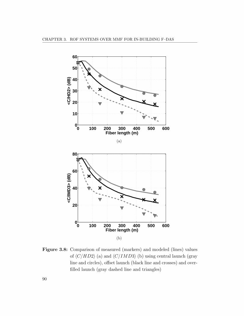
CHAPTER 3. ROF SYSTEMS OVER MMF FOR IN-BUILDING F–DAS
0 100 200 300 400 500 6000
10
20
30
40
50
60
Fiber length (m)
<C/H
D2>
(d
B)
(a)
0 100 200 300 400 500 6000
20
40
60
80
Fiber length (m)
<C/IM
D3>
(d
B)
(b)
Figure 3.8: Comparison of measured (markers) and modeled (lines) values
of 〈C/HD2〉 (a) and 〈C/IMD3〉 (b) using central launch (gray
line and circles), offset launch (black line and crosses) and over-
filled launch (gray dashed line and triangles)
90
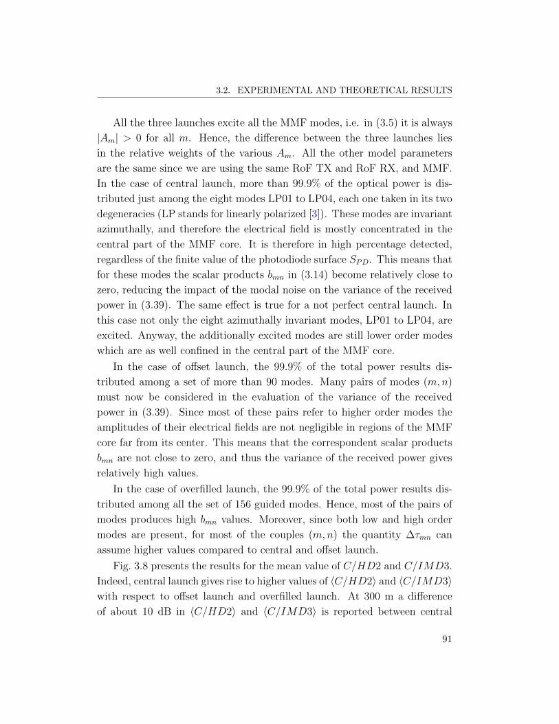
3.2. EXPERIMENTAL AND THEORETICAL RESULTS
All the three launches excite all the MMF modes, i.e. in (3.5) it is always
|Am| > 0 for all m. Hence, the difference between the three launches lies
in the relative weights of the various Am. All the other model parameters
are the same since we are using the same RoF TX and RoF RX, and MMF.
In the case of central launch, more than 99.9% of the optical power is dis-
tributed just among the eight modes LP01 to LP04, each one taken in its two
degeneracies (LP stands for linearly polarized [3]). These modes are invariant
azimuthally, and therefore the electrical field is mostly concentrated in the
central part of the MMF core. It is therefore in high percentage detected,
regardless of the finite value of the photodiode surface SPD. This means that
for these modes the scalar products bmn in (3.14) become relatively close to
zero, reducing the impact of the modal noise on the variance of the received
power in (3.39). The same effect is true for a not perfect central launch. In
this case not only the eight azimuthally invariant modes, LP01 to LP04, are
excited. Anyway, the additionally excited modes are still lower order modes
which are as well confined in the central part of the MMF core.
In the case of offset launch, the 99.9% of the total power results dis-
tributed among a set of more than 90 modes. Many pairs of modes (m,n)
must now be considered in the evaluation of the variance of the received
power in (3.39). Since most of these pairs refer to higher order modes the
amplitudes of their electrical fields are not negligible in regions of the MMF
core far from its center. This means that the correspondent scalar products
bmn are not close to zero, and thus the variance of the received power gives
relatively high values.
In the case of overfilled launch, the 99.9% of the total power results dis-
tributed among all the set of 156 guided modes. Hence, most of the pairs of
modes produces high bmn values. Moreover, since both low and high order
modes are present, for most of the couples (m,n) the quantity ∆τmn can
assume higher values compared to central and offset launch.
Fig. 3.8 presents the results for the mean value of C/HD2 and C/IMD3.
Indeed, central launch gives rise to higher values of 〈C/HD2〉 and 〈C/IMD3〉with respect to offset launch and overfilled launch. At 300 m a difference
of about 10 dB in 〈C/HD2〉 and 〈C/IMD3〉 is reported between central
91
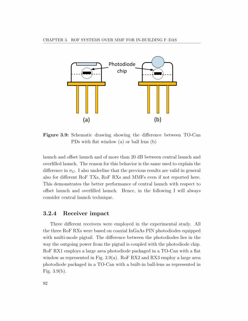
CHAPTER 3. ROF SYSTEMS OVER MMF FOR IN-BUILDING F–DAS
Photodiode
chip
(a) (b)
Figure 3.9: Schematic drawing showing the difference between TO-Can
PDs with flat window (a) or ball lens (b)
launch and offset launch and of more than 20 dB between central launch and
overfilled launch. The reason for this behavior is the same used to explain the
difference in σG. I also underline that the previous results are valid in general
also for different RoF TXs, RoF RXs and MMFs even if not reported here.
This demonstrates the better performance of central launch with respect to
offset launch and overfilled launch. Hence, in the following I will always
consider central launch technique.
3.2.4 Receiver impact
Three different receivers were employed in the experimental study. All
the three RoF RXs were based on coaxial InGaAs PIN photodiodes equipped
with multi-mode pigtail. The difference between the photodiodes lies in the
way the outgoing power from the pigtail is coupled with the photodiode chip.
RoF RX1 employs a large area photodiode packaged in a TO-Can with a flat
window as represented in Fig. 3.9(a). RoF RX2 and RX3 employ a large area
photodiode packaged in a TO-Can with a built-in ball-lens as represented in
Fig. 3.9(b).
92
3.2. EXPERIMENTAL AND THEORETICAL RESULTS
The modeling of the different photodiodes is not trivial since the value of
the illuminated collecting area and the exact coupling scheme between the
pigtail and the photodiode, which is typically done sample by sample, are
both unknown. Hence, a simple equivalent model was used to describe the
reception of the power coming from the MMF. The photodiode was modeled
as a square placed in front of the fiber. The center of the square and the
fiber core center might not coincide, thus a misalignment could be present.
The estimation of side width and misalignment was performed comparing the
received power with central and offset launch with the different receivers and
the values of Γ2DC at different lengths. Then, a least square estimation was
done. The solution, i.e. the values of the pair side width and misalignment,
resulted not uniquely defined. For this reason, the misalignment was set to
1 µm in all the three cases and the side width was consequently estimated.
The side width for the three RoF RXs was: 23 µm for RX1, 26 µm for
RX2, and 28 µm for RX3. As expected, the photodiodes equipped with ball
lens had an equivalent detecting square larger than the photodiode with flat
window. Anyway, the two photodiodes equipped with ball lens have not the
same size of the equivalent square. In particular, RX3 had a larger size of
the equivalent square with respect to RX2.
Fig. 3.10 shows σG between 50 and 550 m for the three different receivers.
The theoretical and experimental curves were obtained using the RoF TX
classified as TX1 in 3.2.5, and central launch. The input power was chosen to
have a OMI per carrier of 0.2. Gray line and circles refer to RoF RX1, blue
line and crosses to RoF RX2, and green line and triangles to RoF RX3. Lines
refer to simulation results while markers refer to measurements. Note that
RoF RX1 gives rise to higher values of σG with respect to RX2. Similarly,
RX2 has higher values of σG with respect to RX3. In particular, at 300 m
there is a difference of 0.25 dB between RX1 and RX2, and of 0.12 dB between
RX2 and RX3.
The reason for this behavior is in the higher equivalent collecting area
of RX3 compared to RX2 and of RX2 compared to RX1. In the numerical
model the impact of the equivalent size of the photodiode is contained in bmn,
expressed in (3.14). Indeed, a larger photodiode area, SPD, reduces the value
93
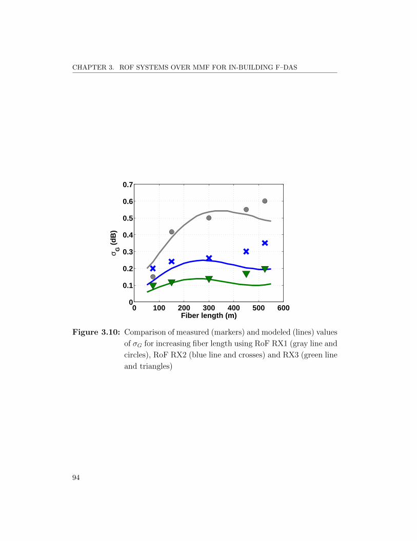
CHAPTER 3. ROF SYSTEMS OVER MMF FOR IN-BUILDING F–DAS
0 100 200 300 400 500 6000
0.1
0.2
0.3
0.4
0.5
0.6
0.7
Fiber length (m)
σ G (
dB
)
Figure 3.10: Comparison of measured (markers) and modeled (lines) values
of σG for increasing fiber length using RoF RX1 (gray line and
circles), RoF RX2 (blue line and crosses) and RX3 (green line
and triangles)
94
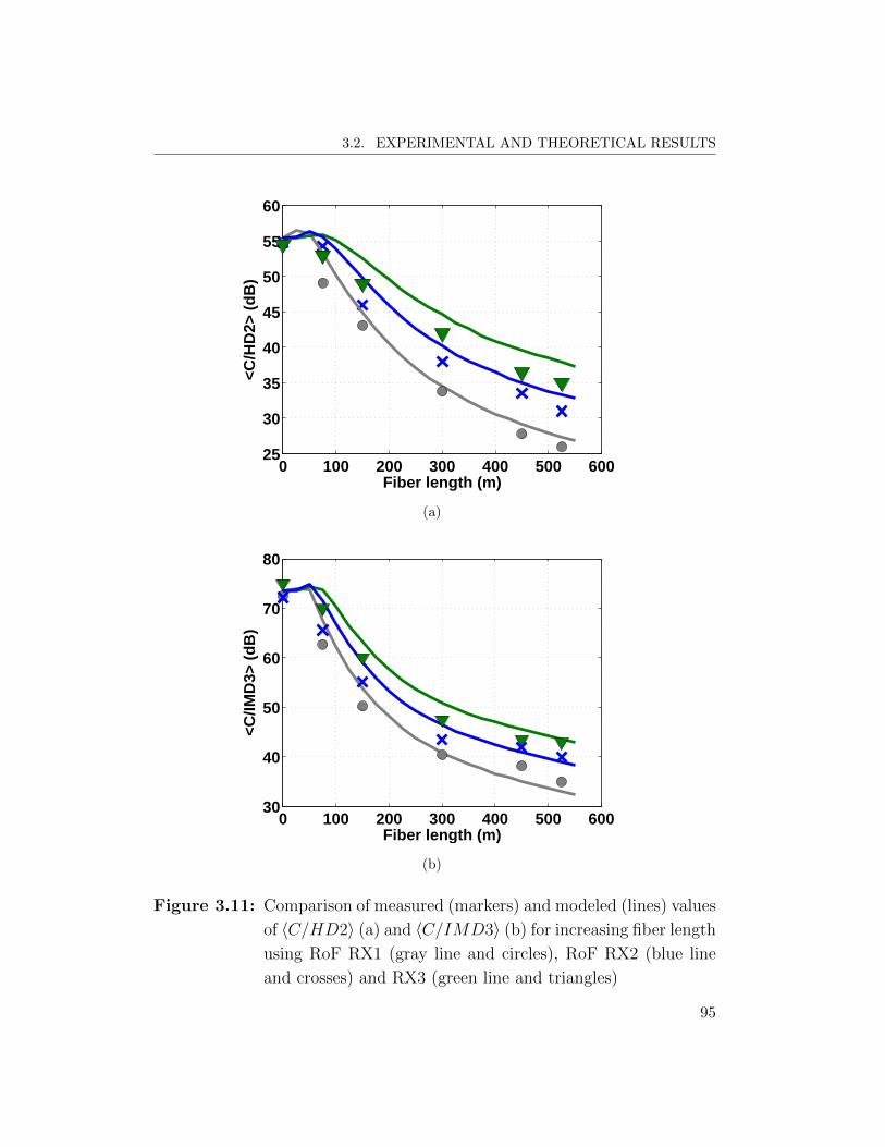
3.2. EXPERIMENTAL AND THEORETICAL RESULTS
0 100 200 300 400 500 60025
30
35
40
45
50
55
60
Fiber length (m)
<C/H
D2>
(d
B)
(a)
0 100 200 300 400 500 60030
40
50
60
70
80
Fiber length (m)
<C/IM
D3>
(d
B)
(b)
Figure 3.11: Comparison of measured (markers) and modeled (lines) values
of 〈C/HD2〉 (a) and 〈C/IMD3〉 (b) for increasing fiber length
using RoF RX1 (gray line and circles), RoF RX2 (blue line
and crosses) and RX3 (green line and triangles)
95

CHAPTER 3. ROF SYSTEMS OVER MMF FOR IN-BUILDING F–DAS
of bmn of all couples, (m,n), of different modes since it is approaching the
ideal case of a large surface where bmn is zero when m 6= n, i.e. orthogonality
of the set of modes. In practice, this situation is not feasible since other causes
of loss of orthogonality such as connector imperfections becomes important
in the determination of modal noise. However, lower values of bmn gives rise
to lower values of the variance of the received power in (3.39).
Fig. 3.11 presents similar results for the mean value of C/HD2 and
C/IMD3. Since the effect of a different photodiode surface impacts on all
the received components in the same way through the coefficients bmn, also in
this case RoF RX1 gives rise to worst 〈C/HD2〉 and 〈C/IMD3〉 compared
to RX2 and the same for RX2 compared to RX3. Since a larger equivalent
area has an impact on all modes, the results presented are not dependent on
the launch or on the transmitter, but are generally valid.
3.2.5 Transmitter impact
The impact on modal noise of the transmitter characteristics is the last
one to be pointed out. I will compare transmitters based on directly mod-
ulated DFB LD and on directly modulated FP LD. In particular, I will
comment on the main transmitter characteristics influencing modal noise.
3.2.5.1 Comparison of transmitters based on DFB laser
Two different RoF TXs based on directly modulated DFB LD were em-
ployed. The modeling parameters of the two TXs are listed in Tab. 3.5. To
give an idea of the dependence of modal noise on these parameters, I will
consider at first a particular condition where the approximation in (3.62)
tends to hold. In this case, the relationship between σG and the transmitter
parameters is,
σG ≈20
ln(10)ΓRF ∝
KfIRFmI
z =Kf
ηTX/P0
z (3.64)
where (3.63) and (3.62) have been used.
96
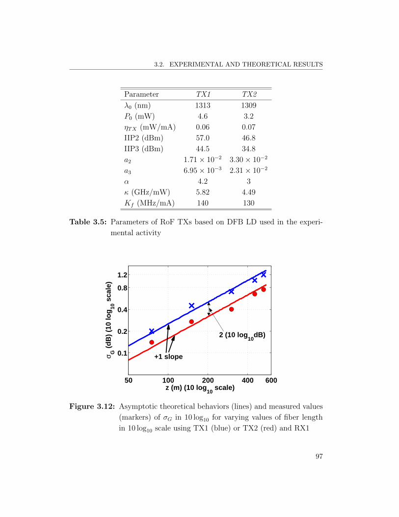
3.2. EXPERIMENTAL AND THEORETICAL RESULTS
Parameter TX1 TX2
λ0 (nm) 1313 1309
P0 (mW) 4.6 3.2
ηTX (mW/mA) 0.06 0.07
IIP2 (dBm) 57.0 46.8
IIP3 (dBm) 44.5 34.8
a2 1.71× 10⁻² 3.30× 10⁻²
a3 6.95× 10⁻³ 2.31× 10⁻²
α 4.2 3
κ (GHz/mW) 5.82 4.49
Kf (MHz/mA) 140 130
Table 3.5: Parameters of RoF TXs based on DFB LD used in the experi-
mental activity
50 100 200 400 600
0.1
0.2
0.4
0.8
1.2
z (m) (10 log10
scale)
σ G (
dB
) (1
0 lo
g10
sca
le)
2 (10 log10
dB)
+1 slope
Figure 3.12: Asymptotic theoretical behaviors (lines) and measured values
(markers) of σG in 10 log10 for varying values of fiber length
in 10 log10 scale using TX1 (blue) or TX2 (red) and RX1
97

CHAPTER 3. ROF SYSTEMS OVER MMF FOR IN-BUILDING F–DAS
To evidence this relationship, Fig. 3.12 shows experimental values and
asymptotic behaviors of σG in 10 log10 scale versus fiber length in 10 log10
scale for TX1 and TX2 in a practical situation where the linear proportion-
ality in (3.64) can be taken with good accuracy. The input power was set to
−4.3 dBm. It was f1 = 700 MHz, f2 = 750 MHz, and the RX1 was used.
Both axes of the graph are in 10 log10 scale to evidence that the asymptotic
curves referred to the two different TXs are parallel with slope +1 and with a
distance of 2 10 log10(dB). Since the only difference in the two cases is given
by the transmitter parameters, this distance can be verified theoretically by,
10 log10 (σG,TX1/σG,TX2) = 10 log10
(Kf,TX1
ηTX1/P0,TX1
/Kf,TX2
ηTX2/P0,TX2
)≈
≈ 2.57 10 log10(dB)
A similar behavior can be determined for the mean values of 〈C/HD2〉and 〈C/IMD3〉. The theoretical expression of the mean value of the received
power at each frequency in (3.34) can be approximated as follows for the
components at fc,1, 2fc,1 and 2fc,2 − fc,1,
〈Pout,fc,1(t)〉 ≈RL
2I2
0m2I
[NM∑m=1
A4mb
2mm + 2
NM−1∑m=1
NM∑n=1
A2mA
2nbmmbnn·
· cos (2πfc,12∆τmn)] (3.65a)
〈Pout,2fc,1(t)〉 ≈RL
2I2
0
a2
2m4I
4
[NM∑m=1
A4mb
2mm + 2
NM−1∑m=1
NM∑n=1
A2mA
2nbmmbnn·
· cos (2π2fc,12∆τmn)] + 8
NM−1∑m=1
NM∑n=1
A2mA
2nb
2mnJ
20 (xmn,2)J2
2 (xmn,1)
(3.65b)
98
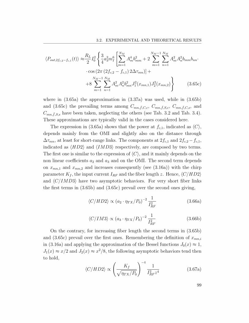
3.2. EXPERIMENTAL AND THEORETICAL RESULTS
〈Pout,2fc,2−fc,1(t)〉 ≈RL
2I2
0
3
4a2
3m6I
[NM∑m=1
A4mb
2mm + 2
NM−1∑m=1
NM∑n=1
A2mA
2nbmmbnn·
· cos (2π (2fc,2 − fc,1) 2∆τmn)] +
+8
NM−1∑m=1
NM∑n=1
A2mA
2nb
2mnJ
21 (xmn,1)J2
2 (xmn,2)
(3.65c)
where in (3.65a) the approximation in (3.37a) was used, while in (3.65b)
and (3.65c) the prevailing terms among Cmn,f ,C,c, Cmn,f ,S,c, Cmn,f ,C,s, and
Cmn,f ,S,s have been taken, neglecting the others (see Tab. 3.2 and Tab. 3.4).
These approximations are typically valid in the cases considered here.
The expression in (3.65a) shows that the power at fc,1, indicated as 〈C〉,depends mainly from the OMI and slightly also on the distance through
∆τmn, at least for short-range links. The components at 2fc,1 and 2fc,2−fc,1,
indicated as 〈HD2〉 and 〈IMD3〉 respectively, are composed by two terms.
The first one is similar to the expression of 〈C〉, and it mainly depends on the
non linear coefficients a2 and a3 and on the OMI. The second term depends
on xmn,1 and xmn,2 and increases consequently (see (3.16a)) with the chirp
parameterKf , the input current IRF and the fiber length z. Hence, 〈C/HD2〉and 〈C/IMD3〉 have two asymptotic behaviors. For very short fiber links
the first terms in (3.65b) and (3.65c) prevail over the second ones giving,
〈C/HD2〉 ∝ (a2 · ηTX/P0)−2 1
I2RF
(3.66a)
〈C/IM3〉 ∝ (a3 · ηTX/P0)−2 1
I2RF
(3.66b)
On the contrary, for increasing fiber length the second terms in (3.65b)
and (3.65c) prevail over the first ones. Remembering the definition of xmn,iin (3.16a) and applying the approximation of the Bessel functions J0(x) ≈ 1,
J1(x) ≈ x/2 and J2(x) ≈ x2/8, the following asymptotic behaviors tend then
to hold,
〈C/HD2〉 ∝
(Kf√ηTX/P0
)−41
I2RF z
4(3.67a)
99
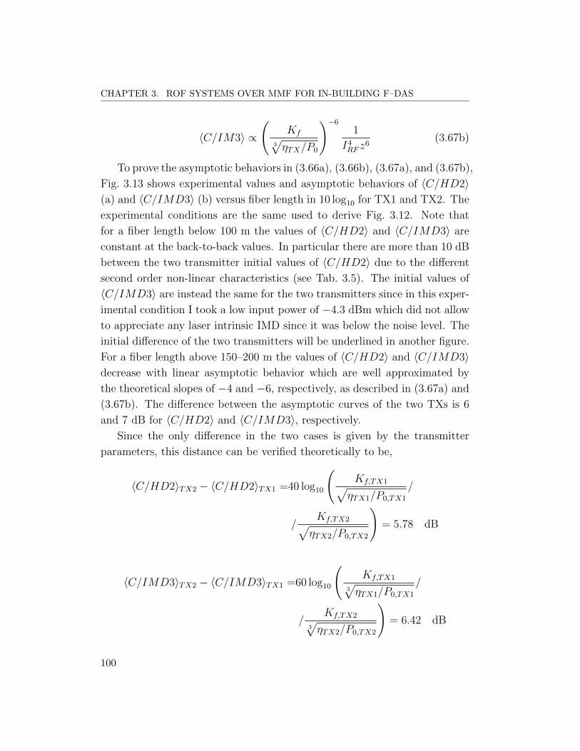
CHAPTER 3. ROF SYSTEMS OVER MMF FOR IN-BUILDING F–DAS
〈C/IM3〉 ∝
(Kf
3√ηTX/P0
)−61
I4RF z
6(3.67b)
To prove the asymptotic behaviors in (3.66a), (3.66b), (3.67a), and (3.67b),
Fig. 3.13 shows experimental values and asymptotic behaviors of 〈C/HD2〉(a) and 〈C/IMD3〉 (b) versus fiber length in 10 log10 for TX1 and TX2. The
experimental conditions are the same used to derive Fig. 3.12. Note that
for a fiber length below 100 m the values of 〈C/HD2〉 and 〈C/IMD3〉 are
constant at the back-to-back values. In particular there are more than 10 dB
between the two transmitter initial values of 〈C/HD2〉 due to the different
second order non-linear characteristics (see Tab. 3.5). The initial values of
〈C/IMD3〉 are instead the same for the two transmitters since in this exper-
imental condition I took a low input power of −4.3 dBm which did not allow
to appreciate any laser intrinsic IMD since it was below the noise level. The
initial difference of the two transmitters will be underlined in another figure.
For a fiber length above 150–200 m the values of 〈C/HD2〉 and 〈C/IMD3〉decrease with linear asymptotic behavior which are well approximated by
the theoretical slopes of −4 and −6, respectively, as described in (3.67a) and
(3.67b). The difference between the asymptotic curves of the two TXs is 6
and 7 dB for 〈C/HD2〉 and 〈C/IMD3〉, respectively.
Since the only difference in the two cases is given by the transmitter
parameters, this distance can be verified theoretically to be,
〈C/HD2〉TX2 − 〈C/HD2〉TX1 =40 log10
(Kf,TX1√
ηTX1/P0,TX1
/
/Kf,TX2√
ηTX2/P0,TX2
)= 5.78 dB
〈C/IMD3〉TX2 − 〈C/IMD3〉TX1 =60 log10
(Kf,TX1
3√ηTX1/P0,TX1
/
/Kf,TX2
3√ηTX2/P0,TX2
)= 6.42 dB
100
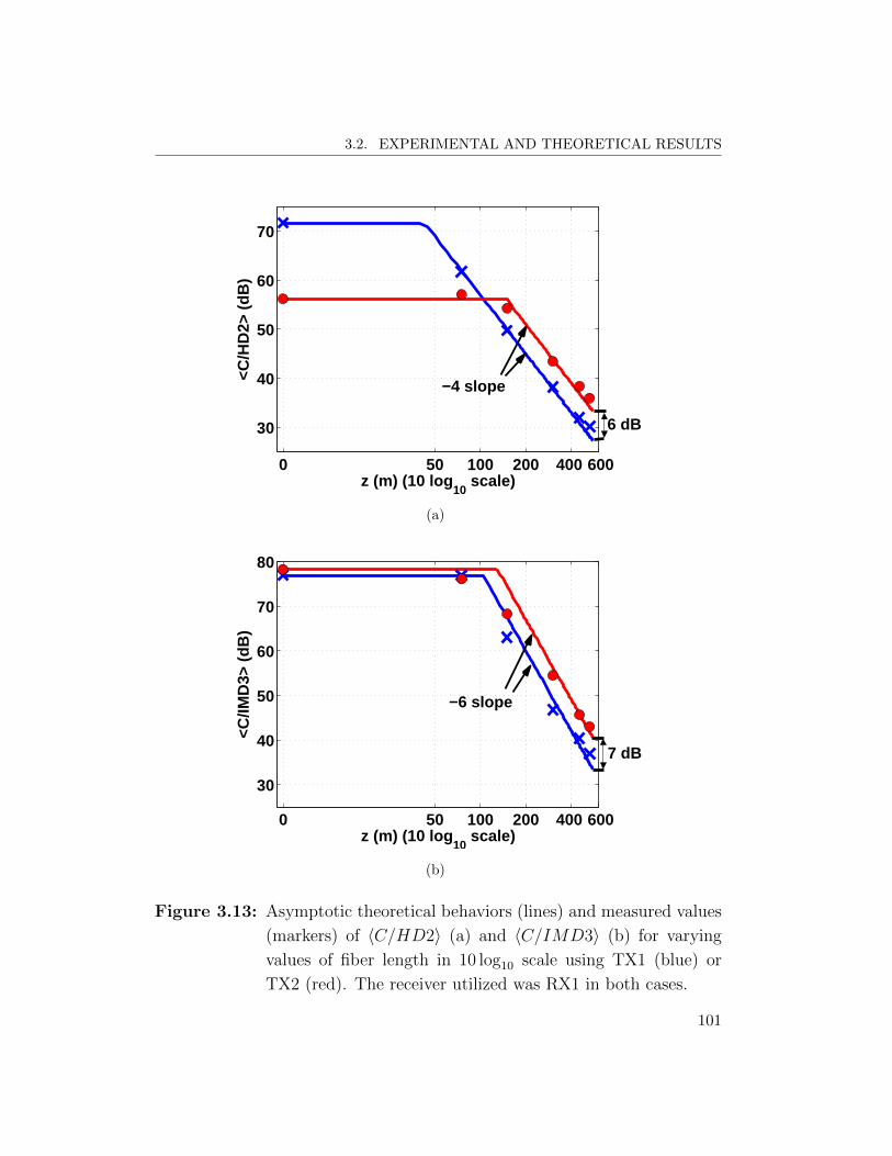
3.2. EXPERIMENTAL AND THEORETICAL RESULTS
0 50 100 200 400 600
30
40
50
60
70
z (m) (10 log10
scale)
<C/H
D2>
(dB
)
−4 slope
6 dB
(a)
0 50 100 200 400 600
30
40
50
60
70
80
z (m) (10 log10
scale)
<C/IM
D3>
(dB
)
7 dB
−6 slope
(b)
Figure 3.13: Asymptotic theoretical behaviors (lines) and measured values
(markers) of 〈C/HD2〉 (a) and 〈C/IMD3〉 (b) for varying
values of fiber length in 10 log10 scale using TX1 (blue) or
TX2 (red). The receiver utilized was RX1 in both cases.
101

CHAPTER 3. ROF SYSTEMS OVER MMF FOR IN-BUILDING F–DAS
0 100 200 300 400 500 6000.05
0.1
0.15
0.2
0.25
0.3
0.35
0.4
Fiber length (m)
σ G (
dB
)
Figure 3.14: Comparison of measured (markers) and modeled (lines) values
of σG for increasing fiber length using RoF TX1 (blue line and
crosses) and RoF TX2 (red line and circles) and RX2
102
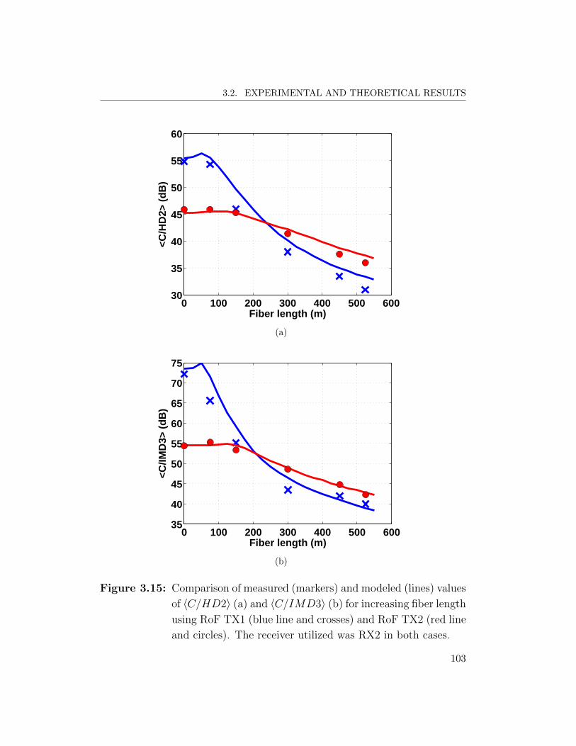
3.2. EXPERIMENTAL AND THEORETICAL RESULTS
0 100 200 300 400 500 60030
35
40
45
50
55
60
Fiber length (m)
<C/H
D2>
(d
B)
(a)
0 100 200 300 400 500 60035
40
45
50
55
60
65
70
75
Fiber length (m)
<C/IM
D3>
(d
B)
(b)
Figure 3.15: Comparison of measured (markers) and modeled (lines) values
of 〈C/HD2〉 (a) and 〈C/IMD3〉 (b) for increasing fiber length
using RoF TX1 (blue line and crosses) and RoF TX2 (red line
and circles). The receiver utilized was RX2 in both cases.
103

CHAPTER 3. ROF SYSTEMS OVER MMF FOR IN-BUILDING F–DAS
The approximated relationships (3.64), (3.67a) and (3.67b) are not strictly
applicable in all the possible operating conditions. Anyway, it is always con-
firmed:
• the decrease of σG with the increase of Kf/(ηTX/P0)
• the decrease of 〈C/HD2〉 with the increase of Kf/√ηTX/P0
• the decrease of 〈C/IMD3〉 with the increase of Kf/3√ηTX/P0
Fig. 3.14 and 3.15 shows experimental and theoretical values of σG, and
〈C/HD2〉 and 〈C/IMD3〉, respectively, for TX1 (blue) and TX2 (red). In
this case the input power was 7.7 dBm, f1 = 1000 MHz and f2 = 1200 MHz,
and the receiver RX2 was used.
Fig. 3.14 demonstrates that σG tends to increase with fiber length and
that TX2 performs better than TX1 of about 0.15 dB above 300 m. Fig. 3.15
shows that 〈C/HD2〉 and 〈C/IMD3〉 start from asymptotic initial values re-
lated to the non-linear characteristics of the TXs (see again Tab. 3.5). In
particular, since TX1 has better non-linear characteristics, the initial values
of 〈C/HD2〉 and 〈C/IMD3〉 are higher than TX2 of 10 dB for 〈C/HD2〉and of 15 dB for 〈C/IMD3〉. However, for increasing fiber length the val-
ues of 〈C/HD2〉 and 〈C/IMD3〉 referred to TX1 sharply decrease and be-
come lower than the respective values referred to TX2. This is due to the
higher value of the parameters Kf/√ηTX/P0 and Kf/
3√ηTX/P0 of TX1 com-
pared to TX2. In particular, there is a difference of 4 dB in 〈C/HD2〉 and
〈C/IMD3〉 between the two TXs performance.
3.2.5.2 Comparison of transmitters based on Fabry-Perot laser
Two different RoF TXs based on directly modulated FP LDs were em-
ployed. The reason to use multi-wavelength sources in RoMMF link is that
a lower coherent laser is expected to reduce the impact of modal noise. Any-
way, to verify this expectation it is important to compare the experimental
and theoretical results obtained for FP sources with the results obtained with
DFB sources. The modeling of the FP RoMMF link was performed using
104
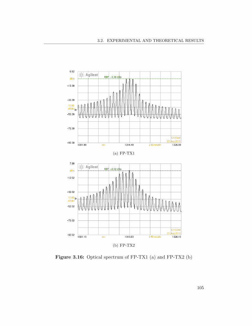
3.2. EXPERIMENTAL AND THEORETICAL RESULTS
(a) FP-TX1
(b) FP-TX2
Figure 3.16: Optical spectrum of FP-TX1 (a) and FP-TX2 (b)
105

CHAPTER 3. ROF SYSTEMS OVER MMF FOR IN-BUILDING F–DAS
Parameter FP-TX1 FP-TX2
Peak wavelength (nm) 1314.5 1313.6
Mode spacing (nm) 0.79 0.8
FWHM (nm) 2.4 3
P0 (mW) 2.3 4.4
ηTX (mW/mA) 0.055 0.08
IIP2 (dBm) 37 45
IIP3 (dBm) 32 40
a2 9.34× 10⁻² 4.92× 10⁻²
a3 3.68× 10⁻² 1.01× 10⁻²
α 8.7 2.4
κ (GHz/mW) 2.25 6.68
Kf (MHz/mA) 120 110
Table 3.6: Parameters of RoF TXs based on DFB LD used in the experi-
mental activity
the model described in subsection 3.1.4. The laser parameters are listed in
Tab. 3.6. The optical spectrum of the two FP TXs is reported in Fig. 3.16.
Note that the optical spectra are composed by many wavelengths, but only
few of them hold the maior part of the power. Indeed, the parameter defined
in (3.50) assumes the following values for the two TXs,∑NW
k=1
(I
(k)0
)2
(∑NWk=1 I
(k)0
)2
FP−TX1
= 0.18 ,
∑NW
k=1
(I
(k)0
)2
(∑NWk=1 I
(k)0
)2
FP−TX2
= 0.15
Since the values of this parameter are between 0.15 and 0.18, this means
that the two FP-TXs are similar to multi-wavelength sources with 5–7 wave-
lengths with identical power. The impact of this characteristic on σG is
shown in Fig. 3.17. In this figure experimental and theoretical values of σGare shown for FP-TX1 (yellow), FP-TX2 (brown) and compared with TX2
(red) of the previous section. These results are obtained with an input power
of 7.7 dBm, f1 = 1000 MHz and f2 = 1200 MHz. The receiver used was RX2.
106
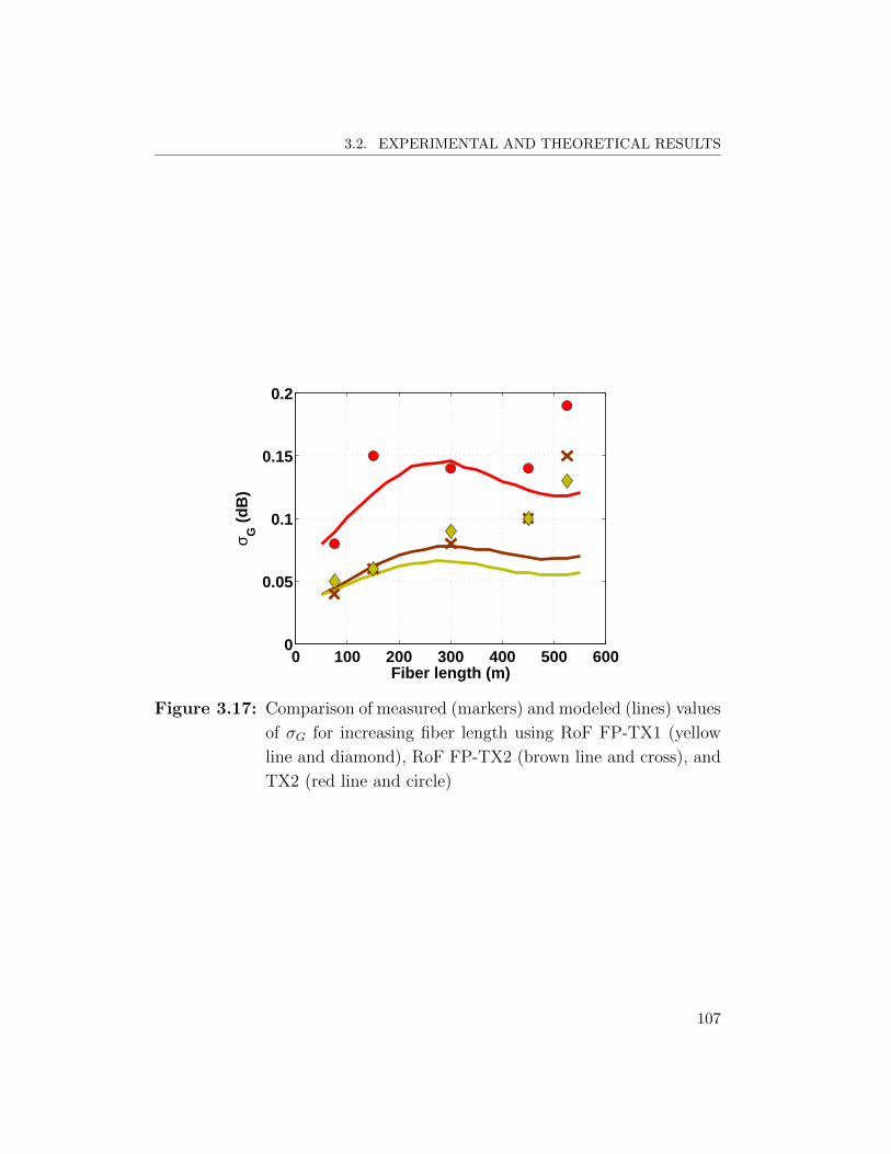
3.2. EXPERIMENTAL AND THEORETICAL RESULTS
0 100 200 300 400 500 6000
0.05
0.1
0.15
0.2
Fiber length (m)
σ G (
dB
)
Figure 3.17: Comparison of measured (markers) and modeled (lines) values
of σG for increasing fiber length using RoF FP-TX1 (yellow
line and diamond), RoF FP-TX2 (brown line and cross), and
TX2 (red line and circle)
107

CHAPTER 3. ROF SYSTEMS OVER MMF FOR IN-BUILDING F–DAS
0 100 200 300 400 500 60034
36
38
40
42
44
46
Fiber length (m)
<C/H
D2>
(d
B)
(a)
0 100 200 300 400 500 60040
45
50
55
60
65
70
Fiber length (m)
<C/IM
D3>
(d
B)
(b)
Figure 3.18: Comparison of measured (markers) and modeled (lines) values
of 〈C/HD2〉 (a) and 〈C/IMD3〉 (b) for increasing fiber length
using RoF FP-TX1 (yellow line and diamond), RoF FP-TX2
(brown line and cross), and TX2 (red line and circle)
108
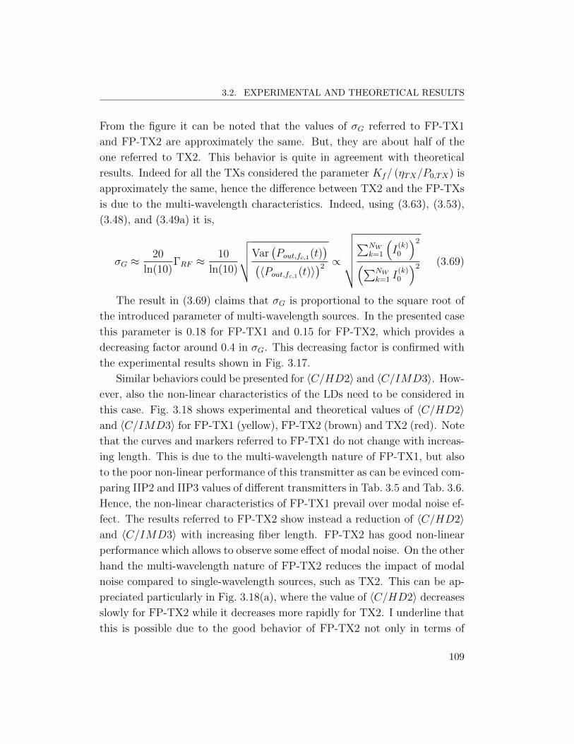
3.2. EXPERIMENTAL AND THEORETICAL RESULTS
From the figure it can be noted that the values of σG referred to FP-TX1
and FP-TX2 are approximately the same. But, they are about half of the
one referred to TX2. This behavior is quite in agreement with theoretical
results. Indeed for all the TXs considered the parameter Kf/ (ηTX/P0,TX) is
approximately the same, hence the difference between TX2 and the FP-TXs
is due to the multi-wavelength characteristics. Indeed, using (3.63), (3.53),
(3.48), and (3.49a) it is,
σG ≈20
ln(10)ΓRF ≈
10
ln(10)
√√√√Var(Pout,fc,1(t)
)(〈Pout,fc,1(t)〉
)2 ∝
√√√√√√∑NW
k=1
(I
(k)0
)2
(∑NWk=1 I
(k)0
)2 (3.69)
The result in (3.69) claims that σG is proportional to the square root of
the introduced parameter of multi-wavelength sources. In the presented case
this parameter is 0.18 for FP-TX1 and 0.15 for FP-TX2, which provides a
decreasing factor around 0.4 in σG. This decreasing factor is confirmed with
the experimental results shown in Fig. 3.17.
Similar behaviors could be presented for 〈C/HD2〉 and 〈C/IMD3〉. How-
ever, also the non-linear characteristics of the LDs need to be considered in
this case. Fig. 3.18 shows experimental and theoretical values of 〈C/HD2〉and 〈C/IMD3〉 for FP-TX1 (yellow), FP-TX2 (brown) and TX2 (red). Note
that the curves and markers referred to FP-TX1 do not change with increas-
ing length. This is due to the multi-wavelength nature of FP-TX1, but also
to the poor non-linear performance of this transmitter as can be evinced com-
paring IIP2 and IIP3 values of different transmitters in Tab. 3.5 and Tab. 3.6.
Hence, the non-linear characteristics of FP-TX1 prevail over modal noise ef-
fect. The results referred to FP-TX2 show instead a reduction of 〈C/HD2〉and 〈C/IMD3〉 with increasing fiber length. FP-TX2 has good non-linear
performance which allows to observe some effect of modal noise. On the other
hand the multi-wavelength nature of FP-TX2 reduces the impact of modal
noise compared to single-wavelength sources, such as TX2. This can be ap-
preciated particularly in Fig. 3.18(a), where the value of 〈C/HD2〉 decreases
slowly for FP-TX2 while it decreases more rapidly for TX2. I underline that
this is possible due to the good behavior of FP-TX2 not only in terms of
109
CHAPTER 3. ROF SYSTEMS OVER MMF FOR IN-BUILDING F–DAS
non-linear characteristics but also linear characteristics, i.e. modulation effi-
ciency, ηTX , and frequency chirping, Kf , which are, respectively, the higher
and the lower among the presented DFB and FP transmitters. This suggests
that FP-TX2 can be successfully applied to a complete RoMMF link.
3.3 LTE transmission experiments
The experimental and theoretical activity presented in the previous sec-
tions was performed to investigate the impact of different quantities of the
link components on the RoMMF link linear and non-linear performances lim-
ited by modal noise. With the results coming from this study it was possible
to develop a cost-effective RoMMF link with good performance. The RoF
TX was based on the FP-TX2 reported in subsection 3.2.5.2 and the launch-
ing technique was central launch since it was proved in subsection 3.2.3 to
provide the best performance. The RoF RX was then equipped by the pho-
todiode with built-in ball lens, addressed as RX3 in subsection 3.2.4,which
showed the best performances. The photodiode was followed by a TIA.
A general characterization of the properties of the designed link was per-
formed in terms of the spurious free dynamic range (SFDR) [52]. SFDR is
an important parameter for analog links which takes into account both the
intermodulation distortion effects and the noise of the entire link. Therefore
it accounts also for noise and intermodulation distortions of the TIA. SFDR
is defined as the ratio between the received power and the noise level in a
1 Hz band when the third-order intermodulation distortions are at the noise
level. It gives an idea of the maximum signal-to-noise ratio achievable by the
link under test, therefore higher values correspond to better performances.
Fig. 3.19 depicts the SFDR of the RoMMF link for increasing fiber length.
In particular, the markers refer to the mean value of SFDR at each distance
and the bars represents the intervals between the 99% minimum and the
99% maximum values. The 99% minimum/maximum is the value which is
exceeded/not exceeded for 99% of time. Note that the mean value of SFDR is
practically invariant with increasing length while the minimum at 99% goes
110

3.3. LTE TRANSMISSION EXPERIMENTS
0 100 200 300 400 500105
107
109
111
113
115
Fiber length (m)
SF
DR
(d
B×H
z2/3 )
99% max value
mean value99% min value
Figure 3.19: SFDR mean and 99% min/max values of the RoMMF link for
increasing MMF fiber
from 110 dB × Hz2/3 for a short fiber length to 105 dB × Hz2/3 after 525 m
MMF. Although there are 5 dB of degradation due to modal noise after
525 m, values of SFDR in excess of 100 dB × Hz2/3 are considered good for
RoMMF systems [35]. This is the result of the careful choice of components
related to the experimental and theoretical activity of the previous sections.
In this section I will show the capability of this cost-effective RoMMF link
to perform the transmission of LTE signals with high quality. The test of
the transmission quality was performed evaluating the ACLR and the error
vector magnitude (EVM) of the received signals. Fig. 3.20 shows the ex-
perimental setup. Two Agilent N9020A MXG VSGs were used to generate
the LTE carriers: one for the downlink (DL) 750 MHz band and one for the
DL 1950 MHz band. For the ACLR test two carriers per band were gener-
ated according to test-model 1.1 for LTE signals with channel bandwidth of
1.4 MHz [82]. The two carriers per band were spaced by 2.8 MHz and cen-
tered at 750 MHz and 1950 MHz. Thus, the two pairs of carrier frequencies
were 748.6 MHz, 751.4 MHz and 1948.6 MHz, 1951.4 MHz, respectively. For
111

CHAPTER 3. ROF SYSTEMS OVER MMF FOR IN-BUILDING F–DAS
VSA
RoF TX RoF RX
VSG 1 – 750 MHz VSG 2 – 1950 MHz
MMF SMF Climatic Chamber
MMF Length z
Connector
+
Figure 3.20: Experimental setup of dual band LTE transmission over the
designed RoMMF link
the EVM test one carrier per band was generated according to test-model
3.1 for LTE signals with channel bandwidth of 20 MHz [82]. The carrier
frequencies were 750 and 1950 MHz. The signals coming from the two VSGs
were combined and applied to the RoF TX. The output power of the two
VSGs was 0 dBm in both tests. At the receiver side an Agilent N5182A
MXA VSA was used to perform the ACLR and the EVM tests.
As discussed regarding Fig. 3.19, the degradation increases with fiber
length. Hence, the ACLR and EVM tests can focus just on the comparison
between the performances in the back-to-back case and after 525 m of MMF.
In the following table the mean value, the 99%maximum and the 99% min-
imum of ACLR are presented for back-to-back and 525 m fiber length for
both bands.
back-to-back 525 m MMF
750 MHz 1950 MHz 750 MHz 1950 MHz
ACLR mean (dBc) -57.14 -60.31 -58.09 -56.64
ACLR 99% max (dBc) -54.26 -57.65 -50.96 -48.14
ACLR 99% min (dBc) -60.47 -63.27 -65.55 -63.87
As can be evinced from the table, the mean value at 750 MHz of the ACLR
in the back-to-back case is comparable with the one after 525 m transmission.
112
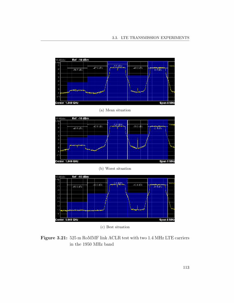
3.3. LTE TRANSMISSION EXPERIMENTS
(a) Mean situation
(b) Worst situation
(c) Best situation
Figure 3.21: 525 m RoMMF link ACLR test with two 1.4 MHz LTE carriers
in the 1950 MHz band
113
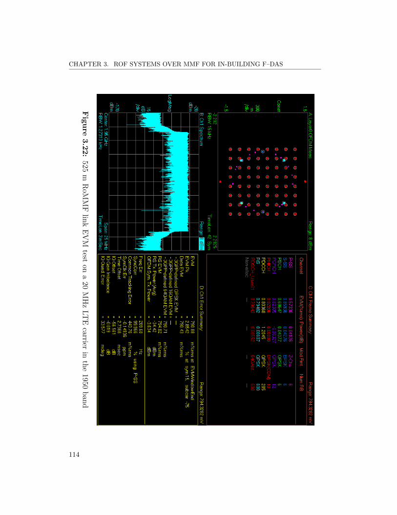
CHAPTER 3. ROF SYSTEMS OVER MMF FOR IN-BUILDING F–DAS
Fig
ure
3.2
2:
525m
RoM
MF
link
EV
Mtest
ona
20M
Hz
LT
Ecarrier
inth
e1950
ban
d
114
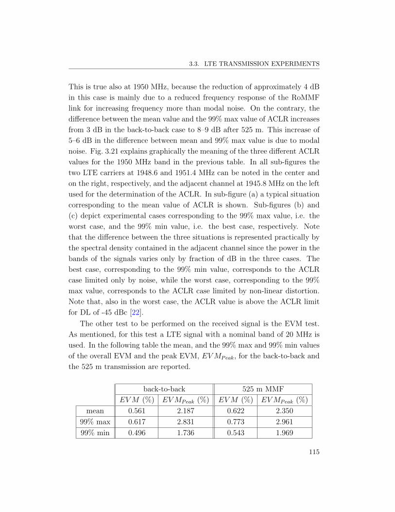
3.3. LTE TRANSMISSION EXPERIMENTS
This is true also at 1950 MHz, because the reduction of approximately 4 dB
in this case is mainly due to a reduced frequency response of the RoMMF
link for increasing frequency more than modal noise. On the contrary, the
difference between the mean value and the 99% max value of ACLR increases
from 3 dB in the back-to-back case to 8–9 dB after 525 m. This increase of
5–6 dB in the difference between mean and 99% max value is due to modal
noise. Fig. 3.21 explains graphically the meaning of the three different ACLR
values for the 1950 MHz band in the previous table. In all sub-figures the
two LTE carriers at 1948.6 and 1951.4 MHz can be noted in the center and
on the right, respectively, and the adjacent channel at 1945.8 MHz on the left
used for the determination of the ACLR. In sub-figure (a) a typical situation
corresponding to the mean value of ACLR is shown. Sub-figures (b) and
(c) depict experimental cases corresponding to the 99% max value, i.e. the
worst case, and the 99% min value, i.e. the best case, respectively. Note
that the difference between the three situations is represented practically by
the spectral density contained in the adjacent channel since the power in the
bands of the signals varies only by fraction of dB in the three cases. The
best case, corresponding to the 99% min value, corresponds to the ACLR
case limited only by noise, while the worst case, corresponding to the 99%
max value, corresponds to the ACLR case limited by non-linear distortion.
Note that, also in the worst case, the ACLR value is above the ACLR limit
for DL of -45 dBc [22].
The other test to be performed on the received signal is the EVM test.
As mentioned, for this test a LTE signal with a nominal band of 20 MHz is
used. In the following table the mean, and the 99% max and 99% min values
of the overall EVM and the peak EVM, EVMPeak, for the back-to-back and
the 525 m transmission are reported.
back-to-back 525 m MMF
EVM (%) EVMPeak (%) EVM (%) EVMPeak (%)
mean 0.561 2.187 0.622 2.350
99% max 0.617 2.831 0.773 2.961
99% min 0.496 1.736 0.543 1.969
115

CHAPTER 3. ROF SYSTEMS OVER MMF FOR IN-BUILDING F–DAS
As shown in the table, the impact of the MMF transmission on the EVM
is negligible both on the overall EVM and the peak EVM. This is due
to the good performance of the designed link and to the small sensitivity
of the OFDMA format, used by a LTE signal, to impairments. Fig. 3.22
renders the typical EVM test corresponding to the max 99% value of the
525 m transmission. The close-to-ideal constellation diagram of the received
64–QAM can be evinced. The same figure contains also the spectrum of the
received signal and more detailed information about the LTE signal reception.
The presented result supports the designed RoMMF link as a viable cost-
effective solutions for present and next-generation F–DAS systems based on
MMF.
3.4 Summary
This chapter presented the modeling and experimental activity on RoMMF
links employing directly modulated DFB and FP lasers. A theoretical model
able to quantify the impact of modal noise on different received frequency
components has been reported in section 3.1 and applied for the analytical
calculation of the some meaningful statistical quantities, i.e. the mean re-
ceived power at each frequency component and the standard deviation of
the DC and the RF components. In section 3.2 an experimental activity
for the determination of the impact of different characteristics of the link
components on link gain, harmonic and intermodulation distortions due to
modal noise has been presented. Some important design guidelines obtained
from experimental results and supported by the developed theory have been
reported. The major detrimental effects of modal noise has been proved to
be adequately controllable with the appliance of central launch technique, a
photodiode with a built-in ball lens, and a FP laser characterized by non-
linear properties, modulation efficiency and frequency chirping competitive
with DFB lasers. The designed RoMMF link was then described and char-
acterized in section 3.3. This link proved to guarantee good performances in
terms of ACLR and EVM up to 525 m when applied to a dual band radio
116

3.4. SUMMARY
transmission of LTE signals.
117

CHAPTER 3. ROF SYSTEMS OVER MMF FOR IN-BUILDING F–DAS
118

Chapter 4POF systems
for home area networks
In this chapter, with the aim to illustrate the applicability of plastic op-
tical fibers to a home area network (HAN), multi-gigabit transmission over
1 mm diameter POF IM–DD links employing a red VCSEL and Si photodi-
odes will be demonstrated. A model for the channel capacity of the POF link
will be described in section 4.1. Experimental results using discrete multi-
tone (DMT) modulation with 2N–quadrature amplitude modulation (QAM)
and bit-loading algorithm will be presented in section 4.2 and compared with
the theoretical capacity. Finally, the positive addition of 3×2N–QAM in the
DMT bit-loading algorithm will be shown in section 4.3.
4.1 Model for the channel capacity of IM–DD
POF links
Plastic optical fibers with a core diameter of approximately 1 mm are a
kind of multimode fibers with more than one million of potentially excited
modes [11]. This large amount of excitable modes together with the use of
This chapter is based on the results published in P6., P10., and P16.
119
CHAPTER 4. POF SYSTEMS FOR HOME AREA NETWORKS
low coherence sources, such as a LED or a VCSEL, reduces at the minimum
level optical interferences effects described in section 3, such as modal noise.
This leads to an initial simplification to the expansion of the detected current
iout with respect to the case of silica MMF.
Starting from (3.19), and neglecting the interference term, we can then
write,
iout(t, z) = I0
NM∑m=1
A2mbmm (1 + y(t− τmz)) (4.1)
In this section broadband digital transmission is considered. Hence, the
modulating signal y(t) in (4.1) can be expressed as,
y(t) = mI · s(t) (4.2)
where s(t) is the normalized signal with max |s(t)| = 1. The last normaliza-
tion is due to the fact that s(t) is a baseband signal for digital transmission,
thus the peak normalization of OMI is employed (see subsection 2.1.1.1).
Substituting (4.2) in (4.1) and considering the relationship in the Fourier
domain, it is,
Iout(f, z) = I0
NM∑m=1
A2mbmmδ (f) +mII0
NM∑m=1
A2mbmm exp (−j2πτmzf)S(f) =
= Iout,0 · δ (f) +H (f)S(f) (4.3)
where Iout(f, z) and S(f) are the Fourier transform of iout(t, z) and s(t),
respectively, and δ (f) is the Dirac delta function.
Apart from the DC component, which can be disregarded using alternating
current (AC) coupling between photodiode and electronics, in (4.3) the spec-
trum of the received current is linearly related with the normalized trans-
mitted signal through the transfer function H (f). Unfortunately, the huge
number of modes present in large core POF causes the determination of the
transfer function starting from an electromagnetic analysis to be very com-
plex. It is then a common approach to describe H (f) by a simplified model,
such as a gaussian or a first order low-pass channel response or to recover it
from measurements [11].
120

4.1. MODEL FOR THE CHANNEL CAPACITY OF IM–DD POF LINKS
To determine the maximum capacity of the channel, C, with a known
transfer function, H(f), and a known noise density it is possible to use the
result coming from the information theory [83, 84],
C ≤∫ +∞
−∞
1
2log2
[1 +
Gs(f) |H(f)|2
N(f)
]df (4.4)
where Gs(f) and N(f) are the spectral densities of the transmitted signal
and of the noise, respectively.
To calculate the capacity in (4.4) it is usually added the power constraint
on the transmitted power Ps ,
Ps =
∫ +∞
−∞Gs(f)df (4.5)
In this derivation, to refer the performance to the received signal-to-noise
ratio (SNR), I will instead force a constraint on the received power PR ,
PR =
∫ +∞
−∞Gs(f) |H(f)|2 df (4.6)
The transmitted power spectral density Gs(f) is the quantity to be opti-
mized. The solution to this optimization problem is obtained with Lagrange
multipliers and the so-called water-filling method. The solution is given by
[83, 84],
Gs(f) =
(ν − N(f)
|H(f)|2
)+
(4.7)
where ν is the ”water-level” to be determined applying the constraint in (4.6)
and (.)+ is the function giving the positive part of its argument,
(x)+ =
x ifx ≥ 0
0 ifx < 0(4.8)
In general there can be more than one interval of frequencies in which the
“water-level” ν is above N(f)/|H(f)|2, and thus Gs(f) is not zeros. However,
assuming that N(f)/|H(f)|2 has an high-pass characteristic, i.e. it increases
121

CHAPTER 4. POF SYSTEMS FOR HOME AREA NETWORKS
ν
B-B
∗
∗ f
Figure 4.1: Water-filling method applied to N(f)/|H(f)|2 with high-pass
characteristic
with increasing frequency, there is only one interval starting from zero and
ending in an unknown maximum bandwidth B in which N(f)/|H(f)|2 is be-
low the “water-level” ν as depicted in Fig. 4.1. This assumption corresponds
to consider H(f) a low-pass transfer function and N(f) increasing with fre-
quency or decreasing less than |H(f)|2. Both assumptions can be taken since
the transfer function of a large core POF has a low-pass characteristics and
the noise spectral density typically increases with frequency. Substituting
(4.7) in (4.6) and applying the previous assumption it is,
PR =
∫ +∞
−∞
(ν − N(f)
|H(f)|2
)+
|H(f)|2 df = 2
∫ B
0+
(ν − N(f)
|H(f)|2
)|H(f)|2 df =
= 2ν
∫ B
0+
|H(f)|2 df − 2
∫ B
0+
N(f)df (4.9)
where the starting point of the integral 0+ denotes that the frequency 0
cannot be used for transmission.
From (4.9) the “water-level” can be determined,
ν =1B
∫ B0+ N(f)df
1B
∫ B0+ |H(f)|2 df
(1 +
PR
2∫ B
0+ N(f)df
)=
1B
∫ B0+ N(f)df
1B
∫ B0+ |H(f)|2 df
(1 + SNR)
(4.10)
122
4.1. MODEL FOR THE CHANNEL CAPACITY OF IM–DD POF LINKS
where SNR is the signal-to-noise ratio at the receiver.
Substituting (4.10) and (4.7) in (4.4), it is,
C ≤∫ B
0+
log2
[1B
∫ B0+ N(f)df
1B
∫ B0+ |H(f)|2 df
(1 + SNR)|H(f)|2
N(f)
]df =
= B log2 (1 + SNR) +B log2
(1
B
∫ B
0+
N(f)
N(B)df
)−∫ B
0+
log2
(N(f)
N(B)
)df −
−B log2
(1
B
∫ B
0+
|H(f)|2 df)
+
∫ B
0+
log2
(|H(f)|2
)df (4.11)
It is important to underline that the bandwidth B in (4.11) depends
from the SNR value. To compare correctly this result with the classical one
and with different channels it is necessary to consider the spectral efficiency
instead of the capacity,
C
B≤ log2 (1 + SNR) + log2
(1
B
∫ B
0+
N(f)
N(B)df
)− 1
B
∫ B
0+
log2
(N(f)
N(B)
)df−
− log2
(1
B
∫ B
0+
|H(f)|2 df)
+1
B
∫ B
0+
log2
(|H(f)|2
)df (4.12)
The first term at the right hand of (4.12) is identical to the Shannon limit
for a non-frequency selective additive white gaussian noise (AWGN) channel.
The other terms represent the amount of difference from the classical limit.
As it is reasonable to suppose, the spectral efficiency of the non-frequency
selective AWGN channel is higher compared to the spectral efficiency of a
low-pass frequency selective AWGN channel, as the one considered here. To
prove this assumption, it is necessary to use the Jensen’s inequality on the
convex function − log2(.) [84],
log2
(1
B
∫ B
0+
N(f)
N(B)df
)− 1
B
∫ B
0+
log2
(N(f)
N(B)
)df ≥ 0 (4.13a)
− log2
(1
B
∫ B
0+
|H(f)|2 df)
+1
B
∫ B
0+
log2
(|H(f)|2
)df ≤ 0 (4.13b)
where the equality holds when N(f) or |H(f)|2 are constant, i.e. white
spectrum over the bandwidth B.
123
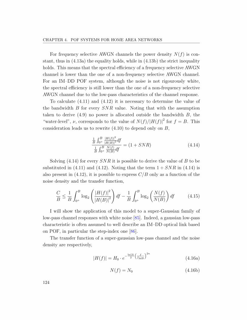
CHAPTER 4. POF SYSTEMS FOR HOME AREA NETWORKS
For frequency selective AWGN channels the power density N(f) is con-
stant, thus in (4.13a) the equality holds, while in (4.13b) the strict inequality
holds. This means that the spectral efficiency of a frequency selective AWGN
channel is lower than the one of a non-frequency selective AWGN channel.
For an IM–DD POF system, although the noise is not rigourously white,
the spectral efficiency is still lower than the one of a non-frequency selective
AWGN channel due to the low-pass characteristics of the channel response.
To calculate (4.11) and (4.12) it is necessary to determine the value of
the bandwidth B for every SNR value. Noting that with the assumption
taken to derive (4.9) no power is allocated outside the bandwidth B, the
“water-level”, ν, corresponds to the value of N(f)/|H(f)|2 for f = B. This
consideration leads us to rewrite (4.10) to depend only on B,
1B
∫ B0+
|H(f)|2
|H(B)|2df
1B
∫ B0+
N(f)N(B)
df= (1 + SNR) (4.14)
Solving (4.14) for every SNR it is possible to derive the value of B to be
substituted in (4.11) and (4.12). Noting that the term 1 + SNR in (4.14) is
also present in (4.12), it is possible to express C/B only as a function of the
noise density and the transfer function,
C
B≤ 1
B
∫ B
0+
log2
(|H(f)|2
|H(B)|2
)df − 1
B
∫ B
0+
log2
(N(f)
N(B)
)df (4.15)
I will show the application of this model to a super-Gaussian family of
low-pass channel responses with white noise [85]. Indeed, a gaussian low-pass
characteristic is often assumed to well describe an IM–DD optical link based
on POF, in particular the step-index one [86].
The transfer function of a super-gaussian low-pass channel and the noise
density are respectively,
|H(f)| = H0 · e− ln(2)
2
(f
f3dB
)2n
(4.16a)
N(f) = N0 (4.16b)
124
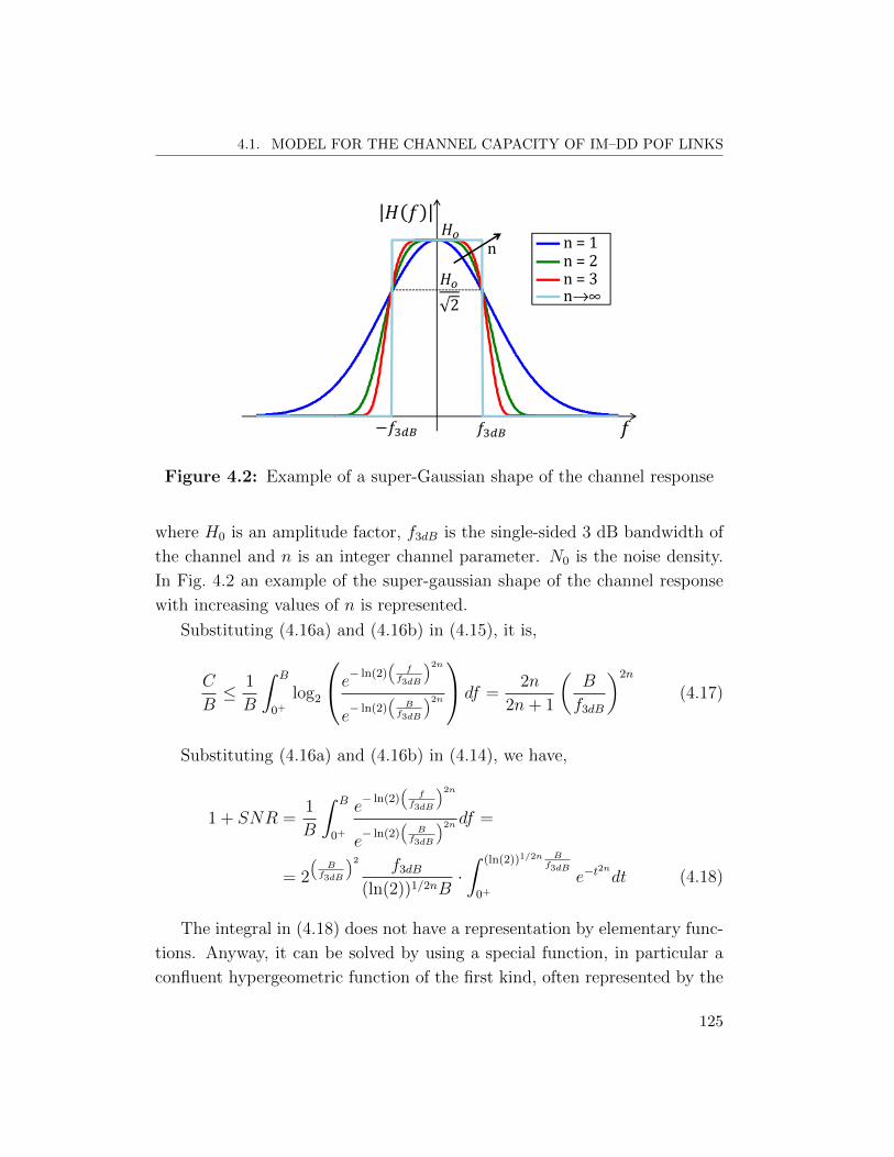
4.1. MODEL FOR THE CHANNEL CAPACITY OF IM–DD POF LINKS
2
−
n = 1
n = 2
n = 3
n→∞
n
Figure 4.2: Example of a super-Gaussian shape of the channel response
where H0 is an amplitude factor, f3dB is the single-sided 3 dB bandwidth of
the channel and n is an integer channel parameter. N0 is the noise density.
In Fig. 4.2 an example of the super-gaussian shape of the channel response
with increasing values of n is represented.
Substituting (4.16a) and (4.16b) in (4.15), it is,
C
B≤ 1
B
∫ B
0+
log2
e− ln(2)(
ff3dB
)2n
e− ln(2)
(B
f3dB
)2n
df =2n
2n+ 1
(B
f3dB
)2n
(4.17)
Substituting (4.16a) and (4.16b) in (4.14), we have,
1 + SNR =1
B
∫ B
0+
e− ln(2)
(f
f3dB
)2n
e− ln(2)
(B
f3dB
)2n df =
= 2
(B
f3dB
)2 f3dB
(ln(2))1/2nB·∫ (ln(2))1/2n B
f3dB
0+
e−t2n
dt (4.18)
The integral in (4.18) does not have a representation by elementary func-
tions. Anyway, it can be solved by using a special function, in particular a
confluent hypergeometric function of the first kind, often represented by the
125

CHAPTER 4. POF SYSTEMS FOR HOME AREA NETWORKS
symbol 1F1(a; b; z) [59]. Indeed, the following integral representation holds,
1F1(a; b; z) =Γ(b)
Γ(b− a)Γ(a)
∫ 1
0
etzta−1(1− t)b−a−1dt (4.19)
where Γ(.) is the Gamma function [59].
After some calculation, using (4.19) it is possible to show that,∫ z
0
e−t2n
dt = ze−z2n
1F1
(1;
2n+ 1
2n; z2n
)(4.20)
Substituting (4.20) in (4.18), it gives us,
1 + SNR = 1F1
(1;
2n+ 1
2n; ln(2) ·
(B
f3dB
)2n)
(4.21)
From (4.21) it is not possible to derive a closed-form relationship of B to
insert in (4.17). However, it is possible to do the reverse operation. Obtaining
B/f3dB from (4.17) and substituting in (4.21) it is,
SNR ≥ 1F1
(1;
2n+ 1
2n; ln(2) · 2n+ 1
2n· CB
)− 1 (4.22)
I underline that (4.22) states that there is a relationship between SNR
and C/B which does not depend on the channel bandwidth f3dB, but only on
its shape. This does not mean that two gaussian channels with different 3 dB
bandwidth give rise to the same capacity, but that for the same SNR the
ratio between the capacity and the used bandwidth for transmission is the
same. This property is generally derivable from (4.12) and (4.14) assuming
a scaling factor in the frequency domain.
Fig. 4.3(a) shows the spectral efficiency of super-gaussian low-pass AWGN
channels with the integer parameter n ranging from 1 to 4, compared with
a flat AWGN channel. As expected, the spectral efficiency of all the super-
gaussian low-pass channels is lower than the spectral efficiency of an AWGN
channel and similar for low SNR value. For increasing values of the inte-
ger parameter n the channel spectral efficiency approaches the flat AWGN
channel limit. This is related to the fact that for increasing values of n the
channel becomes similar to a flat channel with bandwidth B = f3dB.
126
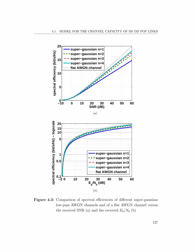
4.1. MODEL FOR THE CHANNEL CAPACITY OF IM–DD POF LINKS
−10 0 10 20 30 40 50 600
5
10
15
20
SNR (dB)
spec
tral
effi
cien
cy (
bit/s
/Hz)
super−gaussian n=1super−gaussian n=2super−gaussian n=3super−gaussian n=4flat AWGN channel
(a)
−2 0 10 20 30 40 50 600.1
0.5
1
5
101525
Eb/N
0 (dB)sp
ectr
al e
ffici
emcy
(bi
t/s/H
z) −
logs
cale
super−gaussian n=1super−gaussian n=2super−gaussian n=3super−gaussian n=4flat AWGN channel
(b)
Figure 4.3: Comparison of spectral efficiencies of different super-gaussian
low-pass AWGN channels and of a flat AWGN channel versus
the received SNR (a) and the received Eb/N0 (b)
127
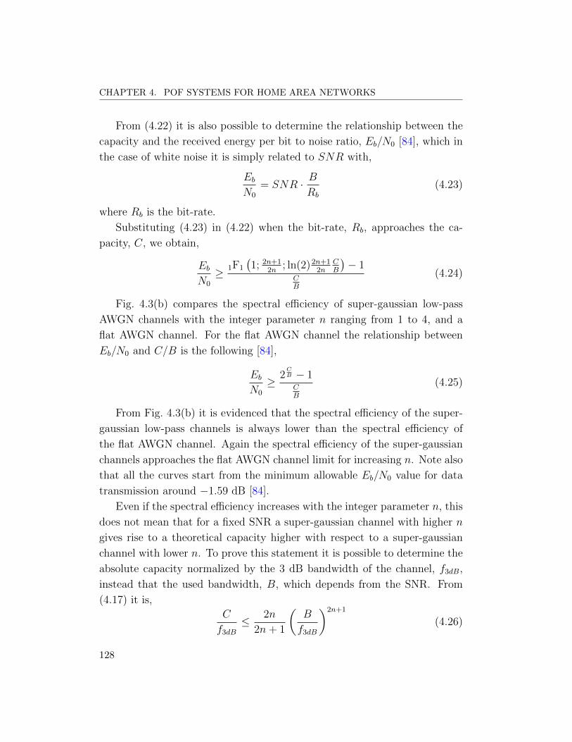
CHAPTER 4. POF SYSTEMS FOR HOME AREA NETWORKS
From (4.22) it is also possible to determine the relationship between the
capacity and the received energy per bit to noise ratio, Eb/N0 [84], which in
the case of white noise it is simply related to SNR with,
EbN0
= SNR · BRb
(4.23)
where Rb is the bit-rate.
Substituting (4.23) in (4.22) when the bit-rate, Rb, approaches the ca-
pacity, C, we obtain,
EbN0
≥ 1F1
(1; 2n+1
2n; ln(2)2n+1
2nCB
)− 1
CB
(4.24)
Fig. 4.3(b) compares the spectral efficiency of super-gaussian low-pass
AWGN channels with the integer parameter n ranging from 1 to 4, and a
flat AWGN channel. For the flat AWGN channel the relationship between
Eb/N0 and C/B is the following [84],
EbN0
≥ 2CB − 1CB
(4.25)
From Fig. 4.3(b) it is evidenced that the spectral efficiency of the super-
gaussian low-pass channels is always lower than the spectral efficiency of
the flat AWGN channel. Again the spectral efficiency of the super-gaussian
channels approaches the flat AWGN channel limit for increasing n. Note also
that all the curves start from the minimum allowable Eb/N0 value for data
transmission around −1.59 dB [84].
Even if the spectral efficiency increases with the integer parameter n, this
does not mean that for a fixed SNR a super-gaussian channel with higher n
gives rise to a theoretical capacity higher with respect to a super-gaussian
channel with lower n. To prove this statement it is possible to determine the
absolute capacity normalized by the 3 dB bandwidth of the channel, f3dB,
instead that the used bandwidth, B, which depends from the SNR. From
(4.17) it is,
C
f3dB
≤ 2n
2n+ 1
(B
f3dB
)2n+1
(4.26)
128
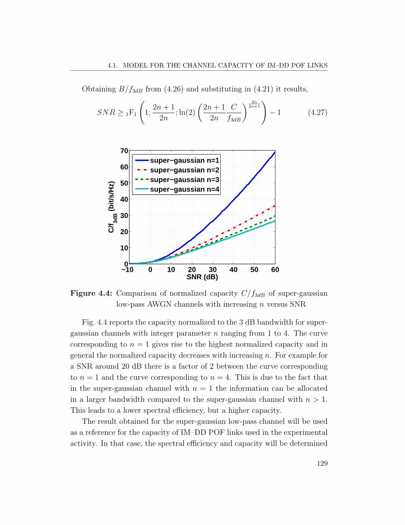
4.1. MODEL FOR THE CHANNEL CAPACITY OF IM–DD POF LINKS
Obtaining B/f3dB from (4.26) and substituting in (4.21) it results,
SNR ≥ 1F1
(1;
2n+ 1
2n; ln(2)
(2n+ 1
2n
C
f3dB
) 2n2n+1
)− 1 (4.27)
−10 0 10 20 30 40 50 600
10
20
30
40
50
60
70
SNR (dB)
C/f
3dB
(bi
t/s/H
z)
super−gaussian n=1super−gaussian n=2super−gaussian n=3super−gaussian n=4
Figure 4.4: Comparison of normalized capacity C/f3dB of super-gaussian
low-pass AWGN channels with increasing n versus SNR
Fig. 4.4 reports the capacity normalized to the 3 dB bandwidth for super-
gaussian channels with integer parameter n ranging from 1 to 4. The curve
corresponding to n = 1 gives rise to the highest normalized capacity and in
general the normalized capacity decreases with increasing n. For example for
a SNR around 20 dB there is a factor of 2 between the curve corresponding
to n = 1 and the curve corresponding to n = 4. This is due to the fact that
in the super-gaussian channel with n = 1 the information can be allocated
in a larger bandwidth compared to the super-gaussian channel with n > 1.
This leads to a lower spectral efficiency, but a higher capacity.
The result obtained for the super-gaussian low-pass channel will be used
as a reference for the capacity of IM–DD POF links used in the experimental
activity. In that case, the spectral efficiency and capacity will be determined
129
CHAPTER 4. POF SYSTEMS FOR HOME AREA NETWORKS
also numerically. I underline that with the described model it is possible
to obtain an upper bound of the real capacity of the channel. Indeed, an
IM–DD POF is not only limited in power, but also in dynamic range. This
means that if the transmitted signal, s(t), with spectral density Gs(f), has
a crest factor, i.e. the ratio of the peak to the root-mean-square amplitude
value of the signal, exceeding the maximum dynamic range, clipping occurs.
However, for POF transmission equal or longer than 50 m the received SNR
with a broadband transmission is typically below 20 dB. For low received
signal power and SNR values the system is much more SNR-limited than
dynamic-range limited, hence the theoretical results maintain a practical
meaning.
4.2 High capacity transmission over GI–POF
employing DMT
In this section I will present IM–DD POF links employing graded-index
POF and two different types of receiver. In subsection 4.2.1 I will shortly in-
troduce DMT and the used bit-loading algorithm. Then, in subsection 4.2.2
I will present the experimental setup and the theoretical maximum perfor-
mance of this links with the model described in section 4.1. In subsec-
tion 4.2.3 and 4.2.4 I will show experimental results related to the application
of DMT modulation with power and bit-loading to obtain multi-gigabit trans-
mission. Finally, I will depict the influence on the main DMT and optical
parameters on the link performance in subsection 4.2.5.
4.2.1 Bit and power loading in DMT
DMT modulation is the baseband version of orthogonal frequency division
multiplexing (OFDM) [87]. It has been widely used in digital subscriber
copper lines for the DSL techniques. The application of this technique to
optical technologies derives from the widespread availability of digital signal
processing (DSP) electronics at affordable prices. The key point to consider
130

4.2. HIGH CAPACITY TRANSMISSION OVER GI–POF EMPLOYING DMT
DMT modulation as a candidate for high-capacity transmission over POF
is the possibility to use a bit and power-loading algorithm which adapts to
the channel. The subcarriers are treated as separate narrowband channels
whose power and modulation can be optimized to fit better the channel
characteristics at the subcarrier frequency. Since the optimization is always
subject to a constraint on the total power, the rate-adaptive bit-loading
problem is a discrete reformulation of the problem expressed by (4.4) and
(4.5). Indicating as N the number of subcarriers, bn and En, respectively,
the number of bits and the energy allocated for the nth subcarrier, it is [88],
maxEn
(b) = maxEn
(N∑n=1
bn
)= max
En
(N∑n=1
log2
(1 +
EngnΓ
))(4.28)
subject toN∑n=1
En = Etot (4.29)
where b is the total numer of bits, gn is the SNR of the nth subcarrier when
unit energy is applied, and Etot is the total available energy.
Γ is the SNR gap, also reported as normalized SNR, which is the difference
in SNR required to achieve maximum capacity as defined by the Shannon
limit at a given error probability.
For M–QAM modulation, the SNR gap, Γ, can be related to the prob-
ability of (two-dimensional) symbol error, Pe, by the following tight upper
bound [89, 90],
Pe ≤ 2 · erfc
(√3
2Γ
)(4.30)
where erfc is the complementary error function [59].
In this work the probability of symbol error is fixed to be 10−3, hence
from the inversion of (4.30) it can be determined Γ ≈ 6 dB. This means
that with M–QAM and probability of symbol error of 10−3, the maximum
achievable capacity is shifted of 6 dB in SNR with respect to the Shannon
limit of the channel.
131
CHAPTER 4. POF SYSTEMS FOR HOME AREA NETWORKS
The bit error rate (BER) related to the symbol error probability of 10−3
depends on the exact modulation and mapping employed, but in any case
it is always less than the symbol error probability, since a symbol error typ-
ically corresponds to a number of bit errors lower than the number of bits
transported by the symbol. However, for real implementation BER of the
order of 10−4 or 10−3 is too high. A forward error correction (FEC) code is
then required to reduced the BER. Focusing on error-free operation, defined
as BER less than 10−12, an enhanced forward error correction (EFEC) code
can be employed to reduce an input BER of up to 3− 4× 10⁻³ to an output
BER below 10−12 at the cost of a 7% redundancy ratio [91].
In the experimental activity I have not implemented the EFEC but I
have considered uncoded performance giving a BER below 10−3 to guarantee
error-free operation when EFEC is inserted.
The solution to the bit-rate maximization problem in (4.28) and (4.29) is
similar to the water-filling method described in section 4.1, and thus it could
be solved with the same technique. However, in this case the optimization
variables En should be choose in order to achieve integer values of bits, bn,
allocated per subcarrier. Among the different algorithm to solve the problem
in (4.28) and (4.29) with finite bit granularity, in this work the Chow’s rate-
adaptive algorithm was employed [92]. The algorithm works as follow [93]:
1. Sort gn in decreasing order, so that g1 is the largest
2. Set btemp(N + 1) = 0 and i = N (btemp(i) and i are the tentative total
bits per subcarrier and number of used subcarriers, respectively)
3. Set equal energy on used tones: En = Etot/i for n = 1, ..., i
4. Compute btemp(i) =∑i
n=1 log2 (1 + Engn/Γ)
5. If btemp(i) < btemp(i + 1), then i ← i + 1 and go to step 6; otherwise
i← i− 1 and go to step 3
6. Compute En = Etot/i and bn = log2 (1 + Engn/Γ) for n = 1, ..., i,
En = 0 and bn = 0 for n = i+ 1, ..., N
132
4.2. HIGH CAPACITY TRANSMISSION OVER GI–POF EMPLOYING DMT
7. Scale En by the factor(2Round(bn) − 1
)/(2bn − 1
)for n = 1, ..., i
(Round(x) is the function giving the nearest integer to x)
8. Compute bn = Round(bn) for n = 1, ..., i
9. Scale En by the factor Etot/(∑i
n=1En
)for n = 1, ..., i
The Chow’s algorithm does not obtain the exact solution of the optimiza-
tion problem in (4.28) and (4.29), but it achieves a near-optimum solution
[93, 92].
Once the number of bits, bn, allocated to the nth subcarrier has been
determined by Chow’s algorithm, the proper modulation scheme can be as-
signed to each subcarrier. Using M–QAM modulation, the nth subcarrier is
allocated with a Mn–QAM modulation where Mn = 2bn . The value En is
used as a pre-emphasis.
4.2.2 Experimental setup
Fig. 4.5 depicts the experimental setup used in this work. The DMT mod-
ulation and demodulation were performed off-line starting from a software de-
veloped in a previous thesis [88]. The transmitted DMT signal was physically
generated by a Tektronix AWG7122B arbitrary waveform generator (AWG)
with 10-bit resolution. The received DMT signal was digitally converted by
a real-time Tektronix DPO72004 digital phosphor oscilloscope (DPO) with
8-bit resolution. The AWG and the DPO were substantially used as the
digital-to-analog converter (DAC) and the analog-to-digital converter (ADC)
elements, respectively. More details on the DMT signal will be reported in
the next sections. The IM–DD POF link was composed by a VCSEL, a
graded-index POF and a receiver based on two different PDs. The VCSEL
was a Firecomms red VCSEL, represented in Fig. 4.6(a), emitting at the
wavelength of 667 nm, with a peak power of 1 mW, a beam divergence of
14 and more than 3 GHz of modulation bandwidth [94]. Due to the large
beam divergence and the peak power of 1 mW, the VCSEL was compliant
with eye-safety regulations [95]. The emitted light from the VCSEL was cou-
pled directly in free space with the GI-POF. I employed different lengths
133

CHAPTER 4. POF SYSTEMS FOR HOME AREA NETWORKS
DAC VCSEL 667nm
Bias
PMMA GI-POF
Arbitrary Waveform Generator
TX sample rate
Tektronix AWG7122B
Real-time Oscilloscope
RX sample rate
Tektronix DPO72004
ADC
DMT Tx
DMT Rx
Off-line processing
Si-PD
Figure 4.5: Experimental setup
mm!
mm!
0 5 10 15 20 25 30 0 5 10 15 20 25 30 35
(a) VCSEL
TIA
PD
0 1 2 3 4 5 0 1 2 3 4 5
mm
mm
(b) Si-PIN PD
Figure 4.6: Photos of the red VCSEL (a) and the receiver based on the
Si-PIN PD (b) used in the experimental setup
134
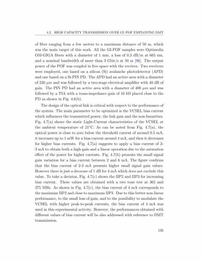
4.2. HIGH CAPACITY TRANSMISSION OVER GI–POF EMPLOYING DMT
of fiber ranging from a few meters to a maximum distance of 50 m, which
was the main target of this work. All the GI-POF samples were Optimedia
OM-GIGA fibers with a diameter of 1 mm, a loss of 0.3 dB/m at 665 nm,
and a nominal bandwidth of more than 3 Gbit/s at 50 m [96]. The output
power of the POF was coupled in free space with the receiver. Two receivers
were employed, one based on a silicon (Si) avalanche photodetector (APD)
and one based on a Si-PIN PD. The APD had an active area with a diameter
of 230 µm and was followed by a two-stage electrical amplifier with 40 dB of
gain. The PIN PD had an active area with a diameter of 400 µm and was
followed by a TIA with a trans-impedance gain of 10 kΩ placed close to the
PD as shown in Fig. 4.6(b).
The design of the optical link is critical with respect to the performance of
the system. The main parameter to be optimized is the VCSEL bias current
which influences the transmitted power, the link gain and the non-linearities.
Fig. 4.7(a) shows the static Light-Current characteristics of the VCSEL at
the ambient temperature of 21C. As can be noted from Fig. 4.7(a), the
optical power is close to zero below the threshold current of around 0.5 mA,
it increases up to 1 mW for a bias current around 4 mA, and then it decreases
for higher bias currents. Fig. 4.7(a) suggests to apply a bias current of 2-
3 mA to obtain both a high gain and a linear operation due to the saturation
effect of the power for higher currents. Fig. 4.7(b) presents the small signal
gain variation for a bias current between 2 and 6 mA. The figure confirms
that the bias current of 2-3 mA presents higher small signal gain values.
However there is just a decrease of 1 dB for 4 mA which does not exclude this
value. To take a decision, Fig. 4.7(c) shows the IIP2 and IIP3 for increasing
bias current. These values are obtained with a two tone test at 365 and
375 MHz. As shown in Fig. 4.7(c), the bias current of 4 mA corresponds to
the maximum IIP2 and close to maximum IIP3. Due to this better non-linear
performance, to the small loss of gain, and to the possibility to modulate the
VCSEL with higher peak-to-peak currents, the bias current of 4 mA was
used in this experimental activity. However, the performances obtained with
different values of bias current will be also addressed with reference to DMT
transmission.
135

CHAPTER 4. POF SYSTEMS FOR HOME AREA NETWORKS
0 1 2 3 4 5 6 7 80
0.2
0.4
0.6
0.8
1
Bias current (mA)
Op
tica
l po
wer
(m
W)
(a) Optical power
2 3 4 5 6−4
−3
−2
−1
0
Bias current (mA)
Nor
mal
ized
sm
all s
igna
l gai
n (d
B)
(b) Normalized small signal gain
2 3 4 5 65
10
15
20
25
Bias current (mA)
IIP2
/ IIP
3 (d
Bm
)
IIP2IIP3
(c) IIP2 / IIP3
Figure 4.7: Optical emitted power (a), normalized small signal gain (b),
and IIP2 / IIP3 (dBm) versus VCSEL bias current
136

4.2. HIGH CAPACITY TRANSMISSION OVER GI–POF EMPLOYING DMT
0 0.5 1 1.5 2 2.5 3−60
−50
−40
−30
−20
−10
0
Frequency (GHz)Nor
mal
ized
freq
uenc
y re
spon
se (
dB)
back−to−back Si−PIN50 m GI−POF Si−PINgauss. n=1, f
3dB= 1.15 GHz
gauss. n=1, f3dB
= 0.76 GHz
back−to−back
50 m
(a) PIN-PD
0 0.5 1 1.5 2 2.5 3−60
−50
−40
−30
−20
−10
0
Frequency (GHz)Nor
mal
ized
freq
uenc
y re
spon
se (
dB)
back−to−back SI−APD50 m GI−POF Si−APDgauss. n=2 f
3dB=1.36 GHz
gauss. n=2 f3dB
=1.31 GHz
back−to−back
50 m
(b) APD
Figure 4.8: Normalized frequency response of the POF link using PIN-PD
(a) or APD (b) for back-to-back and 50 m transmission, and
best super-gaussian interpolating functions
137

CHAPTER 4. POF SYSTEMS FOR HOME AREA NETWORKS
−10 −5 0 5 10 15 20 25 300
2
4
6
8
10
SNR (dB)
spec
tral
effi
cien
cy (
bit/s
/Hz)
50 m POF Si−APD50 m POF Si−PINgauss. n=2, f
3dB=1.31 GHz
gauss. n=1, f3dB
=0.76 GHz
flat AWGN channel
APD
PIN−PD
(a)
−10 −5 0 5 10 15 20 25 300
5
10
15
20
SNR (dB)
Cap
acity
(G
bit/s
)
50 m POF Si−APD50 m POF Si−PINgauss. n=2,f
3dB=1.31 GHz
gauss. n=1,f3dB
=0.76 GHz
APD
PIN−PD
(b)
Figure 4.9: Comparison of spectral efficiency (a) and capacity (b) of the
50 m POF link employing PIN-PD orAPD, and of the best
super-gaussian interpolating functions
138
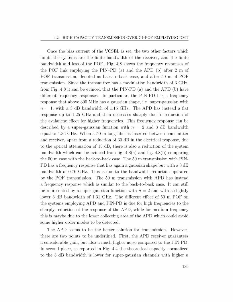
4.2. HIGH CAPACITY TRANSMISSION OVER GI–POF EMPLOYING DMT
Once the bias current of the VCSEL is set, the two other factors which
limits the systems are the finite bandwidth of the receiver, and the finite
bandwidth and loss of the POF. Fig. 4.8 shows the frequency responses of
the POF link employing the PIN–PD (a) and the APD (b) after 2 m of
POF transmission, denoted as back-to-back case, and after 50 m of POF
transmission. Since the transmitter has a modulation bandwidth of 3 GHz,
from Fig. 4.8 it can be evinced that the PIN-PD (a) and the APD (b) have
different frequency responses. In particular, the PIN-PD has a frequency
response that above 300 MHz has a gaussian shape, i.e. super-gaussian with
n = 1, with a 3 dB bandwidth of 1.15 GHz. The APD has instead a flat
response up to 1.25 GHz and then decreases sharply due to reduction of
the avalanche effect for higher frequencies. This frequency response can be
described by a super-gaussian function with n = 2 and 3 dB bandwidth
equal to 1.36 GHz. When a 50 m long fiber is inserted between transmitter
and receiver, apart from a reduction of 30 dB in the electrical response, due
to the optical attenuation of 15 dB, there is also a reduction of the system
bandwidth which can be evinced from fig. 4.8(a) and fig. 4.8(b) comparing
the 50 m case with the back-to-back case. The 50 m transmission with PIN-
PD has a frequency response that has again a gaussian shape but with a 3 dB
bandwidth of 0.76 GHz. This is due to the bandwidth reduction operated
by the POF transmission. The 50 m transmission with APD has instead
a frequency response which is similar to the back-to-back case. It can still
be represented by a super-gaussian function with n = 2 and with a slightly
lower 3 dB bandwidth of 1.31 GHz. The different effect of 50 m POF on
the systems employing APD and PIN-PD is due for high frequencies to the
sharply reduction of the response of the APD, while for medium frequency
this is maybe due to the lower collecting area of the APD which could avoid
some higher order modes to be detected.
The APD seems to be the better solution for transmission. However,
there are two points to be underlined. First, the APD receiver guarantees
a considerable gain, but also a much higher noise compared to the PIN-PD.
In second place, as reported in Fig. 4.4 the theoretical capacity normalized
to the 3 dB bandwidth is lower for super-gaussian channels with higher n
139
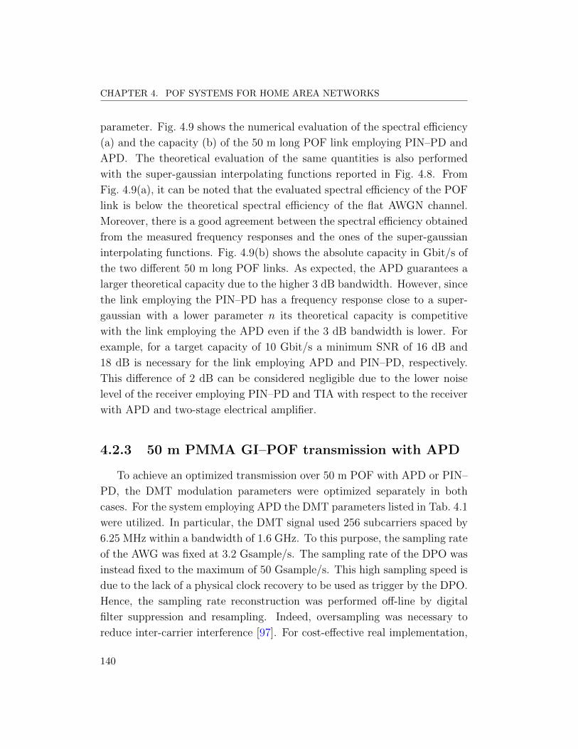
CHAPTER 4. POF SYSTEMS FOR HOME AREA NETWORKS
parameter. Fig. 4.9 shows the numerical evaluation of the spectral efficiency
(a) and the capacity (b) of the 50 m long POF link employing PIN–PD and
APD. The theoretical evaluation of the same quantities is also performed
with the super-gaussian interpolating functions reported in Fig. 4.8. From
Fig. 4.9(a), it can be noted that the evaluated spectral efficiency of the POF
link is below the theoretical spectral efficiency of the flat AWGN channel.
Moreover, there is a good agreement between the spectral efficiency obtained
from the measured frequency responses and the ones of the super-gaussian
interpolating functions. Fig. 4.9(b) shows the absolute capacity in Gbit/s of
the two different 50 m long POF links. As expected, the APD guarantees a
larger theoretical capacity due to the higher 3 dB bandwidth. However, since
the link employing the PIN–PD has a frequency response close to a super-
gaussian with a lower parameter n its theoretical capacity is competitive
with the link employing the APD even if the 3 dB bandwidth is lower. For
example, for a target capacity of 10 Gbit/s a minimum SNR of 16 dB and
18 dB is necessary for the link employing APD and PIN–PD, respectively.
This difference of 2 dB can be considered negligible due to the lower noise
level of the receiver employing PIN–PD and TIA with respect to the receiver
with APD and two-stage electrical amplifier.
4.2.3 50 m PMMA GI–POF transmission with APD
To achieve an optimized transmission over 50 m POF with APD or PIN–
PD, the DMT modulation parameters were optimized separately in both
cases. For the system employing APD the DMT parameters listed in Tab. 4.1
were utilized. In particular, the DMT signal used 256 subcarriers spaced by
6.25 MHz within a bandwidth of 1.6 GHz. To this purpose, the sampling rate
of the AWG was fixed at 3.2 Gsample/s. The sampling rate of the DPO was
instead fixed to the maximum of 50 Gsample/s. This high sampling speed is
due to the lack of a physical clock recovery to be used as trigger by the DPO.
Hence, the sampling rate reconstruction was performed off-line by digital
filter suppression and resampling. Indeed, oversampling was necessary to
reduce inter-carrier interference [97]. For cost-effective real implementation,
140
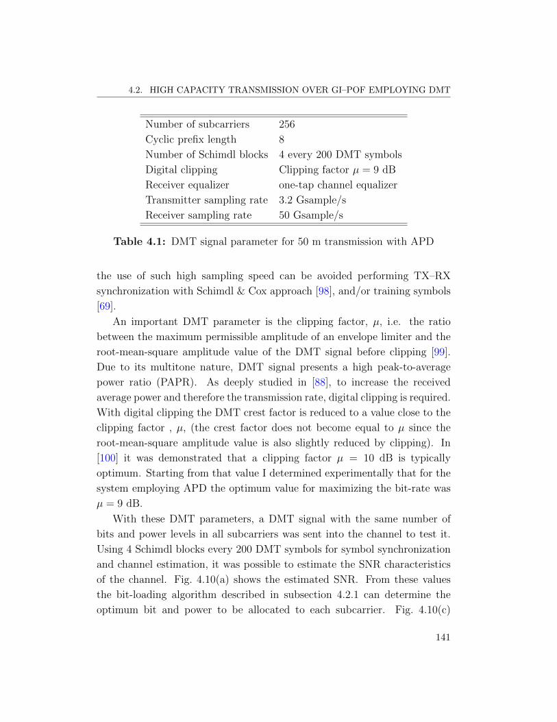
4.2. HIGH CAPACITY TRANSMISSION OVER GI–POF EMPLOYING DMT
Number of subcarriers 256
Cyclic prefix length 8
Number of Schimdl blocks 4 every 200 DMT symbols
Digital clipping Clipping factor µ = 9 dB
Receiver equalizer one-tap channel equalizer
Transmitter sampling rate 3.2 Gsample/s
Receiver sampling rate 50 Gsample/s
Table 4.1: DMT signal parameter for 50 m transmission with APD
the use of such high sampling speed can be avoided performing TX–RX
synchronization with Schimdl & Cox approach [98], and/or training symbols
[69].
An important DMT parameter is the clipping factor, µ, i.e. the ratio
between the maximum permissible amplitude of an envelope limiter and the
root-mean-square amplitude value of the DMT signal before clipping [99].
Due to its multitone nature, DMT signal presents a high peak-to-average
power ratio (PAPR). As deeply studied in [88], to increase the received
average power and therefore the transmission rate, digital clipping is required.
With digital clipping the DMT crest factor is reduced to a value close to the
clipping factor , µ, (the crest factor does not become equal to µ since the
root-mean-square amplitude value is also slightly reduced by clipping). In
[100] it was demonstrated that a clipping factor µ = 10 dB is typically
optimum. Starting from that value I determined experimentally that for the
system employing APD the optimum value for maximizing the bit-rate was
µ = 9 dB.
With these DMT parameters, a DMT signal with the same number of
bits and power levels in all subcarriers was sent into the channel to test it.
Using 4 Schimdl blocks every 200 DMT symbols for symbol synchronization
and channel estimation, it was possible to estimate the SNR characteristics
of the channel. Fig. 4.10(a) shows the estimated SNR. From these values
the bit-loading algorithm described in subsection 4.2.1 can determine the
optimum bit and power to be allocated to each subcarrier. Fig. 4.10(c)
141
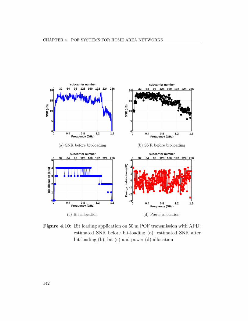
CHAPTER 4. POF SYSTEMS FOR HOME AREA NETWORKS
0 0.4 0.8 1.2 1.60
5
10
15
20
Frequency (GHz)
SN
R (
dB
)
0 32 64 96 128 160 192 224 256subcarrier number
(a) SNR before bit-loading
0 0.4 0.8 1.2 1.60
5
10
15
20
Frequency (GHz)
SN
R (
dB
)
0 32 64 96 128 160 192 224 256subcarrier number
(b) SNR before bit-loading
0 0.4 0.8 1.2 1.60
1
2
3
4
5
Frequency (GHz)
Bit
allo
cati
on
(b
its)
0 32 64 96 128 160 192 224 256subcarrier number
(c) Bit allocation
0 0.4 0.8 1.2 1.6−3
−2
−1
0
1
2
3
Frequency (GHz)
Ene
rgy
dist
ribut
ion
(dB
)
0 32 64 96 128 160 192 224 256subcarrier number
(d) Power allocation
Figure 4.10: Bit loading application on 50 m POF transmission with APD:
estimated SNR before bit-loading (a), estimated SNR after
bit-loading (b), bit (c) and power (d) allocation
142
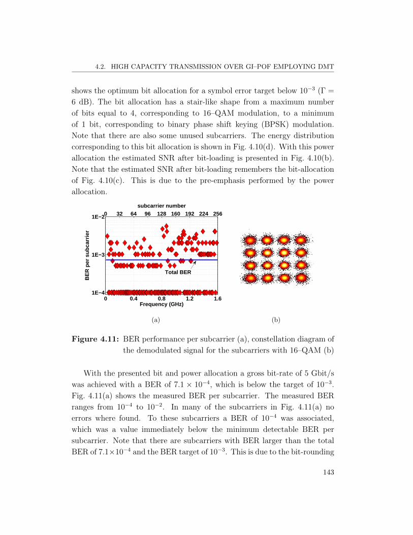
4.2. HIGH CAPACITY TRANSMISSION OVER GI–POF EMPLOYING DMT
shows the optimum bit allocation for a symbol error target below 10−3 (Γ =
6 dB). The bit allocation has a stair-like shape from a maximum number
of bits equal to 4, corresponding to 16–QAM modulation, to a minimum
of 1 bit, corresponding to binary phase shift keying (BPSK) modulation.
Note that there are also some unused subcarriers. The energy distribution
corresponding to this bit allocation is shown in Fig. 4.10(d). With this power
allocation the estimated SNR after bit-loading is presented in Fig. 4.10(b).
Note that the estimated SNR after bit-loading remembers the bit-allocation
of Fig. 4.10(c). This is due to the pre-emphasis performed by the power
allocation.
0 0.4 0.8 1.2 1.61E−4
1E−3
1E−2
Frequency (GHz)
BE
R p
er s
ubca
rrie
r
0 32 64 96 128 160 192 224 256subcarrier number
Total BER
(a) (b)
Figure 4.11: BER performance per subcarrier (a), constellation diagram of
the demodulated signal for the subcarriers with 16–QAM (b)
With the presented bit and power allocation a gross bit-rate of 5 Gbit/s
was achieved with a BER of 7.1 × 10⁻⁴, which is below the target of 10−3.
Fig. 4.11(a) shows the measured BER per subcarrier. The measured BER
ranges from 10−4 to 10−2. In many of the subcarriers in Fig. 4.11(a) no
errors where found. To these subcarriers a BER of 10−4 was associated,
which was a value immediately below the minimum detectable BER per
subcarrier. Note that there are subcarriers with BER larger than the total
BER of 7.1×10⁻⁴ and the BER target of 10−3. This is due to the bit-rounding
143
CHAPTER 4. POF SYSTEMS FOR HOME AREA NETWORKS
in the bit-loading algorithm. However, DMT modulation provides the benefit
to achieve a total average BER below the target BER even in presence of some
subcarriers above that limit. Fig. 4.11(b) shows the superimposed equalized
constellation diagram of all the subcarriers with 16–QAM, corresponding to 4
allocated bits. The clearly distinguishable constellation points indicate that
the received signal quality is high enough to guarantee sufficient performance
also with a simple one-tap channel equalizer.
The previous bit-rate value of 5 Gbit/s must be intended as gross because
it considers as useful information also the Schimdl blocks and the cyclic pre-
fix. Accounting correctly for cyclic prefix and Schimdl blocks, an overhead
of 3.6% needs to be removed from the gross bit-rate. This leads to a un-
coded net bit-rate of 4.85 Gbit/s, corresponding to a spectral efficiency of
3 bit/s/Hz. Accounting also for a 6.7% EFEC overhead, the net bit-rate for
error-free operation becomes 4.55 Gbit/s.
It is possible to compare the obtained bit-rate with the theoretical capac-
ity of the system presented in Fig. 4.9(b).To this purpose, we should compare
the uncoded net bit-rate with the theoretical capacity corresponding to the
measured SNR reduced by the SNR gap, Γ, of 6 dB. Since the overall mea-
sured SNR is 15.5 dB, the capacity corresponding to 9.5 dB should be taken.
From Fig. 4.9(b) this capacity is 5.6 Gbit/s. Therefore, the obtained bit-rate
is 0.75 Gbit/s far from the theoretical capacity achievable by M–QAM.
4.2.4 50 m PMMA GI–POF transmission with PIN PD
For the system employing PIN–PD the parameters listed in Tab. 4.2 were
utilized. The DMT signal used 256 subcarriers spaced by 8.79 MHz within a
bandwidth of 2.25 GHz. The sampling rate of the AWG and the DPO were
fixed at 4.5 and 50 Gsample/s, respectively. For this system the optimum
clipping factor was found to be µ = 8 dB.
Fig. 4.12(a) and 4.12(b) show the estimated SNR before and after bit-
loading, respectively. Note that the SNR of the system employing PIN–PD is
slightly higher than the corresponding SNR of the system employing APD.
This is due to the larger area of the PD and to a lower noise level. Due
144

4.2. HIGH CAPACITY TRANSMISSION OVER GI–POF EMPLOYING DMT
0 0.5 1 1.5 2 2.250
5
10
15
20
25
Frequency (GHz)
SN
R (
dB
)
0 32 64 96 128 160 192 224 256subcarrier number
(a) SNR before bit-loading
0 0.5 1 1.5 2 2.250
5
10
15
20
25
Frequency (GHz)
SN
R (
dB
)
0 32 64 96 128 160 192 224 256subcarrier number
(b) SNR before bit-loading
0 0.5 1 1.5 2 2.250
1
2
3
4
5
Frequency (GHz)
Bit
allo
cati
on
(b
its)
0 32 64 96 128 160 192 224 256subcarrier number
(c) Bit allocation
0 0.5 1 1.5 2 2.25−3
−2
−1
0
1
2
3
Frequency (GHz)
Ene
rgy
dist
ribut
ion
(dB
)
0 32 64 96 128 160 192 224 256subcarrier number
(d) Power allocation
Figure 4.12: Bit loading application on 50 m POF transmission with PIN–
PD: estimated SNR before bit-loading (a), estimated SNR
after bit-loading (b), bit (c) and power (d) allocation
145

CHAPTER 4. POF SYSTEMS FOR HOME AREA NETWORKS
Number of subcarriers 256
Cyclic prefix length 8
Number of Schimdl blocks 2 every 200 DMT symbols
Digital clipping Clipping factor µ = 8 dB
Receiver equalizer one-tap channel equalizer
Transmitter sampling rate 4.5 Gsample/s
Receiver sampling rate 50 Gsample/s
Table 4.2: DMT modulator and demodulator parameter for 50 m transmis-
sion with PIN–PD
to the higher SNR, up to 5 bits, corresponding to 32–QAM modulation,
are allocated. Note that after 1.42 GHz (subcarrier number 162) no bits
are allocated due to low SNR values. For this reason in Fig. 4.12(b) the
SNR after bit-loading can only be evaluated up to 1.42 GHz. The energy
distribution corresponding to the bit allocation is shown in Fig. 4.12(d).
0 0.5 1 1.5 2 2.251E−4
1E−3
1E−2
Frequency (GHz)
BE
R p
er s
ubca
rrie
r
0 32 64 96 128 160 192 224 256subcarrier number
Total BER
(a) (b)
Figure 4.13: BER performance per subcarrier (a), constellation diagram of
the demodulated signal for the subcarriers with 32–QAM (b)
With the optimum bit and power allocation a gross bit-rate of 5.3 Gbit/s
was achieved with a BER of 8.5 × 10⁻⁴, which is below the target of 10−3.
146

4.2. HIGH CAPACITY TRANSMISSION OVER GI–POF EMPLOYING DMT
Fig. 4.13(a) shows the measured BER per subcarrier. As for the APD system,
the BER per subcarrier ranges from 10−4 to 10−2, where the value 10−4
is associated to the subcarrier where no errors were found. Also in this
case, there are subcarriers with BER larger than the target BER of 10−3
mitigated by the DMT signal averaging property. Fig. 4.13(b) shows the
superimposed equalized constellation diagram of all the subcarriers with 32–
QAM, corresponding to 5 allocated bits.
Accounting for cyclic prefix and Schimdl blocks within the gross bit-
rate of 5.3 Gbit/s, the uncoded net bit-rate is 5.15 Gbit/s, corresponding
to a spectral efficiency of 3.6 bit/s/Hz. Accounting also for a 6.7% EFEC
overhead, the net bit-rate for error-free operation becomes 4.85 Gbit/s.
The overall SNR is 17 dB. Hence, to compare the uncoded net bit-rate
with the theoretical capacity of the system the capacity corresponding to a
SNR of 11 dB should be taken. From Fig. 4.9(b) this capacity is 5.4 Gbit/s,
meaning that the obtained net bit-rate is only 0.25 Gbit/s far from the max-
imum capacity achievable with M–QAM.
Summarizing, even if the the 3 dB bandwidth of the system employing
PIN–PD is lower than the 3 dB bandwidth of the system employing APD,
the resulting data-rate is higher. This is due to the use of a matched PD–
TIA receiver which guarantees a high sensitivity and a receiver bandwidth
competitive with the APD solution.
4.2.5 Evaluation of DMT and optical link parameters
The results shown in subsections 4.2.3 and 4.2.4 refer to the transmission
over 50 m GI-POF with all parameters optimized. To prove that the cho-
sen parameters are optimum and to determine the impact of a not optimum
choice, in this section I will show the effect on the link performance of devia-
tion of these parameters from their optimal values. In particular, I will show
the dependencies of the total bit-rate on different values of the number of
subcarriers, the clipping level, the laser bias current, fiber length and bend-
ing loss. The link performance is expressed by the bit-rate deviation from
147
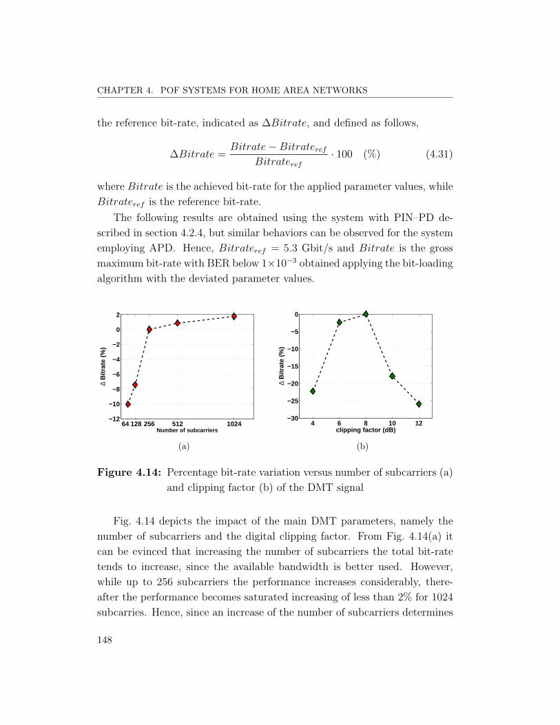
CHAPTER 4. POF SYSTEMS FOR HOME AREA NETWORKS
the reference bit-rate, indicated as ∆Bitrate, and defined as follows,
∆Bitrate =Bitrate−Bitrateref
Bitrateref· 100 (%) (4.31)
where Bitrate is the achieved bit-rate for the applied parameter values, while
Bitrateref is the reference bit-rate.
The following results are obtained using the system with PIN–PD de-
scribed in section 4.2.4, but similar behaviors can be observed for the system
employing APD. Hence, Bitrateref = 5.3 Gbit/s and Bitrate is the gross
maximum bit-rate with BER below 1×10⁻³ obtained applying the bit-loading
algorithm with the deviated parameter values.
64 128 256 512 1024−12
−10
−8
−6
−4
−2
0
2
Number of subcarriers
∆ B
itrat
e (%
)
(a)
4 6 8 10 12−30
−25
−20
−15
−10
−5
0
clipping factor (dB)
∆ B
itrat
e (%
)
(b)
Figure 4.14: Percentage bit-rate variation versus number of subcarriers (a)
and clipping factor (b) of the DMT signal
Fig. 4.14 depicts the impact of the main DMT parameters, namely the
number of subcarriers and the digital clipping factor. From Fig. 4.14(a) it
can be evinced that increasing the number of subcarriers the total bit-rate
tends to increase, since the available bandwidth is better used. However,
while up to 256 subcarriers the performance increases considerably, there-
after the performance becomes saturated increasing of less than 2% for 1024
subcarries. Hence, since an increase of the number of subcarriers determines
148

4.2. HIGH CAPACITY TRANSMISSION OVER GI–POF EMPLOYING DMT
higher complexity and latency, a compromise is required. For this reason,
choosing 256 subcarriers is the optimum compromise for the case considered.
Fig. 4.14(b) shows ∆Bitrate against the clipping factor. For the 50 m
transmission described in subsections 4.2.4 a clipping factor of 8 dB was used,
which from Fig. 4.14(b) is demonstrated to be optimum. But, note that a
clipping factor between 6 and 8 dB gives close to optimum results. For lower
values of clipping factor the clipping noise increases substantially providing
a reduction of the bit-rate [101]. For higher values of clipping factor, due
to a fixed peak-to-peak amplitude of the modulating current to avoid laser
clipping, the average received power decreases resulting in a reduction of the
SNR and hence of the bit-rate. I remark that the crest factor of the DMT
signal without digital clipping would be around 14–15 dB which results in
more than 30% reduction in bit-rate.
Besides number of subcarriers and clipping factor, which are the main
parameters of the DMT signal and can be controlled in the DSP, I analyze
the impact of some other parameters of the optical link. In particular, the
driving bias current of the VCSEL, the POF length and the bending loss of
the POF are examined.
I showed in subsection 4.2.2 that the VCSEL bias current was set to
4 mA based on considerations on the transmitted power, the link gain and
the non-linearities. For further clarification, Fig. 4.15(a) depicts ∆Bitrate
versus the bias current of the VCSEL. The optimum bias current value of
4 mA is confirmed. For low bias currents, the link performance is dominated
by laser clipping leading to asymmetric clipping noise on the received DMT
signal which reduces the achievable bit-rate. For high bias currents the SNR
reduction due to a lower system gain and optical power reduces as well the
achievable bit-rate.
Fig. 4.15(b) presents ∆Bitrate variation with POF link ranging from 10
to 50 m. Since the reference bit-rate is the one at the longest length of
50 m, ∆Bitrate is always positive. At 10 m a relative increase around 43%
is obtained with respect to the 50 m case. Note that Fig. 4.15(b) shows a
linear relationship between ∆Bitrate and fiber length with a negative slope
of −1.1 %/m. This linear relationship is due to the high loss (0.3 dB/m) of
149

CHAPTER 4. POF SYSTEMS FOR HOME AREA NETWORKS
2 3 4 5 6−30
−25
−20
−15
−10
−5
0
Bias current (mA)
∆ B
itrat
e (%
)
(a)
5 10 15 20 25 30 35 40 45 500
10
20
30
40
50
Fiber length (m)
∆ B
itra
te (
%)
(b)
Figure 4.15: Percentage bit-rate variation versus laser bias current (a) and
POF length (b)
5 10 15 20 25 30−100
−80
−60
−40
−20
0
Bending Radius [mm]
∆ B
itrat
e (%
)
5 10 15 20 25 300
2
4
6
8
10
Opt
ical
Los
s (d
B)
Optical Loss∆ Bitrate
Figure 4.16: Percentage bit-rate varation and optical loss versus the bend-
ing radius of a 180 bend
150

4.3. 3× 2N–QAM CONSTELLATIONS FOR DMT
the GI-POF which limits the system by SNR beyond 10 m.
Another important parametric evaluation related to in-field installation
is the bending loss sensitivity of the system. Indeed, GI–POF is today the
large core plastic optical fiber with the highest available bandwidth, but at
the same time it is more sensitive to bending loss with respect to standard
SI–POF [11]. For this reason, Fig. 4.16 presents ∆Bitrate variation due to
decreasing bending radius. The experimental values are obtained using a
half bend (180 bend). The optical loss associated to each bending radius is
also reported in Fig. 4.16. No penalty is observed above a bending radius
of 25 mm, which is the nominal allowable bending radius reported for the
sample of GI–POF [96]. A penalty of more than 7% can be observed below
a bending radius of 20 mm. ∆Bitrate decreases linearly coming from 20
to 7.5 mm and then asymptotically decreases below 7.5 mm. Note that
∆Bitrate decrease follows perfectly the increase of the optical bending loss.
4.3 3× 2N–QAM constellations for DMT
The results presented in the previous section where obtained using QAM
constellations with a number of points which is a power of 2 (2N). Using
these constellations it is possible to transport an integer number of bits per
subcarrier. In particular, on the nth subcarrier it is possible to transport a
number of bits bn which satisfy the relation,
bn = log2
(1 +
EngnΓ
)(4.32)
which was implicit in (4.28).
In (4.32), Engn is the SNR produced by the energy En, and can be in-
dicated by SNRn. Hence, from (4.28) it is possible to derive the minimum
SNRn to be able to transport bn bits on the nth subcarrier,
SNRn ≥(2bn − 1
)· Γ (4.33)
For standard M–QAM it is b = log2(M), and for symbol error fixed to
10−3 it is Γ = 6 dB. From (4.33) the minimum SNR necessary to support a
M–QAM modulation is reported in the following table.
151
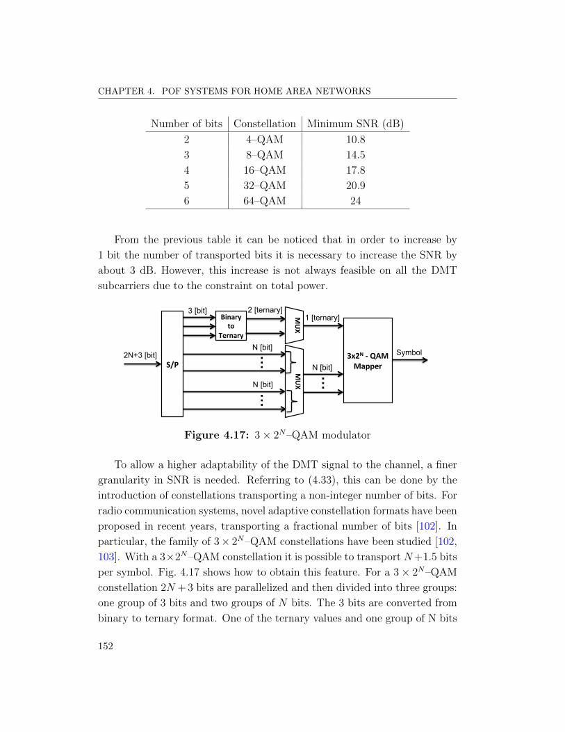
CHAPTER 4. POF SYSTEMS FOR HOME AREA NETWORKS
Number of bits Constellation Minimum SNR (dB)
2 4–QAM 10.8
3 8–QAM 14.5
4 16–QAM 17.8
5 32–QAM 20.9
6 64–QAM 24
From the previous table it can be noticed that in order to increase by
1 bit the number of transported bits it is necessary to increase the SNR by
about 3 dB. However, this increase is not always feasible on all the DMT
subcarriers due to the constraint on total power.
S/P 2N+3 [bit]
3 [bit]
N [bit]
N [bit]
……
Binary to
Ternary
2 [ternary]
MUX
N [bit] …
1 [ternary]
3x2N -‐ QAM Mapper
Symbol
MUX
Figure 4.17: 3× 2N–QAM modulator
To allow a higher adaptability of the DMT signal to the channel, a finer
granularity in SNR is needed. Referring to (4.33), this can be done by the
introduction of constellations transporting a non-integer number of bits. For
radio communication systems, novel adaptive constellation formats have been
proposed in recent years, transporting a fractional number of bits [102]. In
particular, the family of 3× 2N–QAM constellations have been studied [102,
103]. With a 3×2N–QAM constellation it is possible to transport N+1.5 bits
per symbol. Fig. 4.17 shows how to obtain this feature. For a 3× 2N–QAM
constellation 2N + 3 bits are parallelized and then divided into three groups:
one group of 3 bits and two groups of N bits. The 3 bits are converted from
binary to ternary format. One of the ternary values and one group of N bits
152
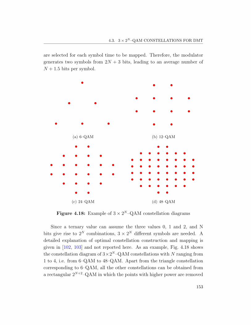
4.3. 3× 2N–QAM CONSTELLATIONS FOR DMT
are selected for each symbol time to be mapped. Therefore, the modulator
generates two symbols from 2N + 3 bits, leading to an average number of
N + 1.5 bits per symbol.
(a) 6–QAM (b) 12–QAM
(c) 24–QAM (d) 48–QAM
Figure 4.18: Example of 3× 2N–QAM constellation diagrams
Since a ternary value can assume the three values 0, 1 and 2, and N
bits give rise to 2N combinations, 3 × 2N different symbols are needed. A
detailed explanation of optimal constellation construction and mapping is
given in [102, 103] and not reported here. As an example, Fig. 4.18 shows
the constellation diagram of 3×2N–QAM constellations with N ranging from
1 to 4, i.e. from 6–QAM to 48–QAM. Apart from the triangle constellation
corresponding to 6–QAM, all the other constellations can be obtained from
a rectangular 2N+2–QAM in which the points with higher power are removed
153
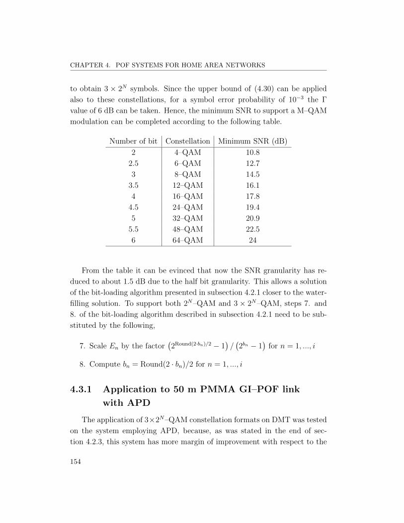
CHAPTER 4. POF SYSTEMS FOR HOME AREA NETWORKS
to obtain 3 × 2N symbols. Since the upper bound of (4.30) can be applied
also to these constellations, for a symbol error probability of 10−3 the Γ
value of 6 dB can be taken. Hence, the minimum SNR to support a M–QAM
modulation can be completed according to the following table.
Number of bit Constellation Minimum SNR (dB)
2 4–QAM 10.8
2.5 6–QAM 12.7
3 8–QAM 14.5
3.5 12–QAM 16.1
4 16–QAM 17.8
4.5 24–QAM 19.4
5 32–QAM 20.9
5.5 48–QAM 22.5
6 64–QAM 24
From the table it can be evinced that now the SNR granularity has re-
duced to about 1.5 dB due to the half bit granularity. This allows a solution
of the bit-loading algorithm presented in subsection 4.2.1 closer to the water-
filling solution. To support both 2N–QAM and 3 × 2N–QAM, steps 7. and
8. of the bit-loading algorithm described in subsection 4.2.1 need to be sub-
stituted by the following,
7. Scale En by the factor(2Round(2·bn)/2 − 1
)/(2bn − 1
)for n = 1, ..., i
8. Compute bn = Round(2 · bn)/2 for n = 1, ..., i
4.3.1 Application to 50 m PMMA GI–POF link
with APD
The application of 3×2N–QAM constellation formats on DMT was tested
on the system employing APD, because, as was stated in the end of sec-
tion 4.2.3, this system has more margin of improvement with respect to the
154
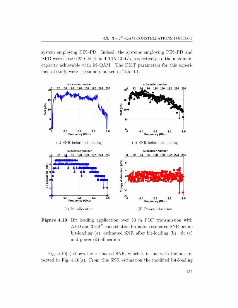
4.3. 3× 2N–QAM CONSTELLATIONS FOR DMT
system employing PIN–PD. Indeed, the systems employing PIN–PD and
APD were close 0.25 Gbit/s and 0.75 Gbit/s, respectively, to the maximum
capacity achievable with M–QAM. The DMT parameters for this experi-
mental study were the same reported in Tab. 4.1.
0 0.4 0.8 1.2 1.60
5
10
15
20
Frequency (GHz)
SN
R (
dB
)
0 32 64 96 128 160 192 224 256subcarrier number
(a) SNR before bit-loading
0 0.4 0.8 1.2 1.60
5
10
15
20
Frequency (GHz)
SN
R (
dB
)
0 32 64 96 128 160 192 224 256subcarrier number
(b) SNR before bit-loading
0 0.4 0.8 1.2 1.60
1
2
3
4
5
Frequency (GHz)
Bit
allo
cati
on
(b
its)
0 32 64 96 128 160 192 224 256subcarrier number
(c) Bit allocation
0 0.4 0.8 1.2 1.6−3
−2
−1
0
1
2
3
Frequency (GHz)
Ene
rgy
dist
ribut
ion
(dB
)
0 32 64 96 128 160 192 224 256subcarrier number
(d) Power allocation
Figure 4.19: Bit loading application over 50 m POF transmission with
APD and 3×2N constellation formats: estimated SNR before
bit-loading (a), estimated SNR after bit-loading (b), bit (c)
and power (d) allocation
Fig. 4.19(a) shows the estimated SNR, which is in-line with the one re-
ported in Fig. 4.10(a). From this SNR estimation the modified bit-loading
155
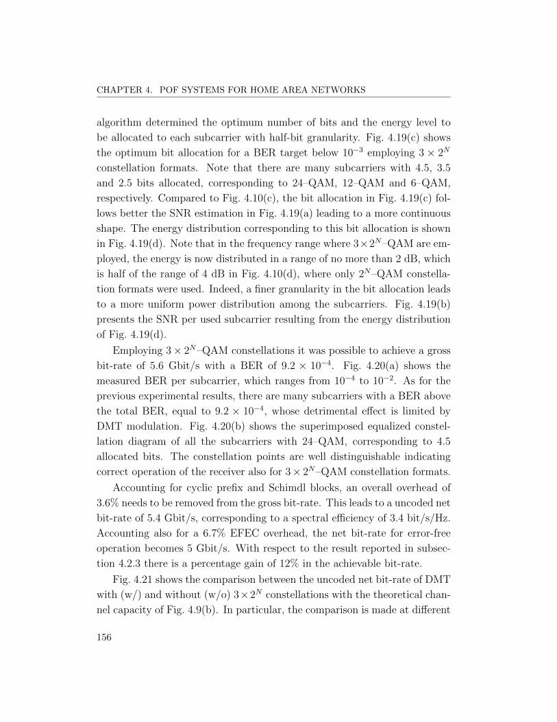
CHAPTER 4. POF SYSTEMS FOR HOME AREA NETWORKS
algorithm determined the optimum number of bits and the energy level to
be allocated to each subcarrier with half-bit granularity. Fig. 4.19(c) shows
the optimum bit allocation for a BER target below 10−3 employing 3 × 2N
constellation formats. Note that there are many subcarriers with 4.5, 3.5
and 2.5 bits allocated, corresponding to 24–QAM, 12–QAM and 6–QAM,
respectively. Compared to Fig. 4.10(c), the bit allocation in Fig. 4.19(c) fol-
lows better the SNR estimation in Fig. 4.19(a) leading to a more continuous
shape. The energy distribution corresponding to this bit allocation is shown
in Fig. 4.19(d). Note that in the frequency range where 3×2N–QAM are em-
ployed, the energy is now distributed in a range of no more than 2 dB, which
is half of the range of 4 dB in Fig. 4.10(d), where only 2N–QAM constella-
tion formats were used. Indeed, a finer granularity in the bit allocation leads
to a more uniform power distribution among the subcarriers. Fig. 4.19(b)
presents the SNR per used subcarrier resulting from the energy distribution
of Fig. 4.19(d).
Employing 3× 2N–QAM constellations it was possible to achieve a gross
bit-rate of 5.6 Gbit/s with a BER of 9.2 × 10⁻⁴. Fig. 4.20(a) shows the
measured BER per subcarrier, which ranges from 10−4 to 10−2. As for the
previous experimental results, there are many subcarriers with a BER above
the total BER, equal to 9.2 × 10⁻⁴, whose detrimental effect is limited by
DMT modulation. Fig. 4.20(b) shows the superimposed equalized constel-
lation diagram of all the subcarriers with 24–QAM, corresponding to 4.5
allocated bits. The constellation points are well distinguishable indicating
correct operation of the receiver also for 3× 2N–QAM constellation formats.
Accounting for cyclic prefix and Schimdl blocks, an overall overhead of
3.6% needs to be removed from the gross bit-rate. This leads to a uncoded net
bit-rate of 5.4 Gbit/s, corresponding to a spectral efficiency of 3.4 bit/s/Hz.
Accounting also for a 6.7% EFEC overhead, the net bit-rate for error-free
operation becomes 5 Gbit/s. With respect to the result reported in subsec-
tion 4.2.3 there is a percentage gain of 12% in the achievable bit-rate.
Fig. 4.21 shows the comparison between the uncoded net bit-rate of DMT
with (w/) and without (w/o) 3×2N constellations with the theoretical chan-
nel capacity of Fig. 4.9(b). In particular, the comparison is made at different
156
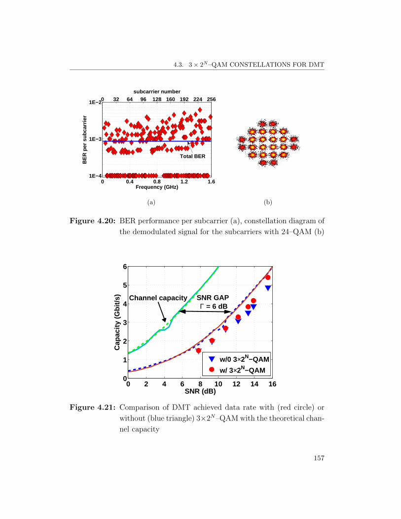
4.3. 3× 2N–QAM CONSTELLATIONS FOR DMT
0 0.4 0.8 1.2 1.61E−4
1E−3
1E−2
Frequency (GHz)
BE
R p
er s
ubca
rrie
r
0 32 64 96 128 160 192 224 256subcarrier number
Total BER
(a) (b)
Figure 4.20: BER performance per subcarrier (a), constellation diagram of
the demodulated signal for the subcarriers with 24–QAM (b)
0 2 4 6 8 10 12 14 160
1
2
3
4
5
6
SNR (dB)
Cap
acity
(G
bit/s
)
w/0 3×2N−QAM
w/ 3×2N−QAM
SNR GAP Γ = 6 dB
Channel capacity
Figure 4.21: Comparison of DMT achieved data rate with (red circle) or
without (blue triangle) 3×2N–QAM with the theoretical chan-
nel capacity
157

CHAPTER 4. POF SYSTEMS FOR HOME AREA NETWORKS
received SNR obtained by decreasing the received optical power always after
50 m of POF transmission. From the figure it can be evinced that for SNR
below 10 dB the two types of DMT signal give similar values since none or
few subcarriers are allocated with 3 × 2N–QAM constellations. Then, for
increasing values of SNR 3× 2N–QAM constellation formats begin to be al-
located to a larger number of subcarriers, leading to an over-performance of
the DMT signal employing 3 × 2N–QAM constellations with respect to the
DMT signal employing only 2N–QAM constellations.
The obtained results are also compared with the theoretical capacity
shifted by the SNR gap Γ = 6 dB. For the SNR of 15.5 dB, correspond-
ing to the results presented in this section, a difference of only 0.2 Gbit/s
from the theoretical capacity shifted by the SNR gap is observed in Fig. 4.21
for the DMT with 3× 2N–QAM constellations. This means that with DMT
modulation employing 3× 2N–QAM constellations, in addition to 2N–QAM,
it is possible to be practically at a distance equal to the SNR gap from the
theoretical channel capacity, which is the minimum distance achievable with
M–QAM.
4.4 Summary
A solution based on plastic optical fiber for the realization of home area
networks has been studied in detail. In this framework, a theoretical and
experimental analysis on the application of DMT to IM–DD GI–POF links
has been presented. Closed-form equations for the capacity of POF links
simplified as super-gaussian AWGN channels were reported in section 4.1
and applied for the description of POF links employing APD and PIN–PD
in subsection 4.2.2.
To use efficiently the non-flat channel response of the POF link, DMT
modulation was employed together with a bit and power loading algorithm
which was described in subsection 4.2.1. The achieved uncoded net bit-rates
were 4.85 and 5.15 Gbit/s for the system employing APD and PIN–PD,
respectively, with optimum parameters. The achieved data-rate are distant
158

4.4. SUMMARY
0.75 and 0.25 Gbit/s, respectively, from the maximum achievable capacity
with M–QAM. To define the effect of non-optimum parameters choice or
real installation conditions, a detailed parametric evaluation was performed
determining also the impact of small bending radii on the POF link.
Finally, 3×2N constellation formats were studied to approach even closer
the maximum achievable capacity with the only limitation of the SNR gap.
Indeed, the half-bit granularity of the bit-loading algorithm exploits at the
best the non-flat channel response. With this scheme the uncoded net bit-rate
of the system employing APD becomes 5.4 Gbit/s which is only 0.2 Gbit/s
from the maximum achievable capacity with M–QAM.
These results demonstrate that DMT can provide close to optimum per-
formance in POF links even with a simple one-tap equalizer and a humble
number of subcarriers such as the 256 employed in this work. Scalability
of these results towards 10 Gbit/s after 50 m POF transmission is feasible
provided that an increase of SNR of at least 6 dB or a receiver based on APD
or PIN–PD with at least double 3 dB bandwidth is realized.
159

CHAPTER 4. POF SYSTEMS FOR HOME AREA NETWORKS
160
Chapter 5POF systems
for converged home networks
As an example of the possibility to use plastic optical fibers for a con-
verged home area network, in this chapter a combined transmission of a
multi-gigabit baseband data stream, based on DMT, and a radio frequency
signal, based on UWB technology, over 1 mm core diameter POF is shown.
After a short introduction on the employed UWB technology in section 5.1,
a detailed experimental study on the performance of the two types of signals
in the combined transmission is carried out in section 5.2.
5.1 Ultra wideband technologies
As already described in section 1.3.2, the near-future indoor scenario
is expected to be full of devices able to transmit with each other. These
devices can use different wireless technologies and some UWB technologies
are expected to be employed especially where reduced energy consumption,
device co-existence and positioning are requested. While narrowband radio
technologies in the ISM band of 2.4 GHz are typically able to transmit up to
tens of meter, UWB technologies are intended to be used below ten meter.
This chapter is based on the results published in P5. and P22.
161
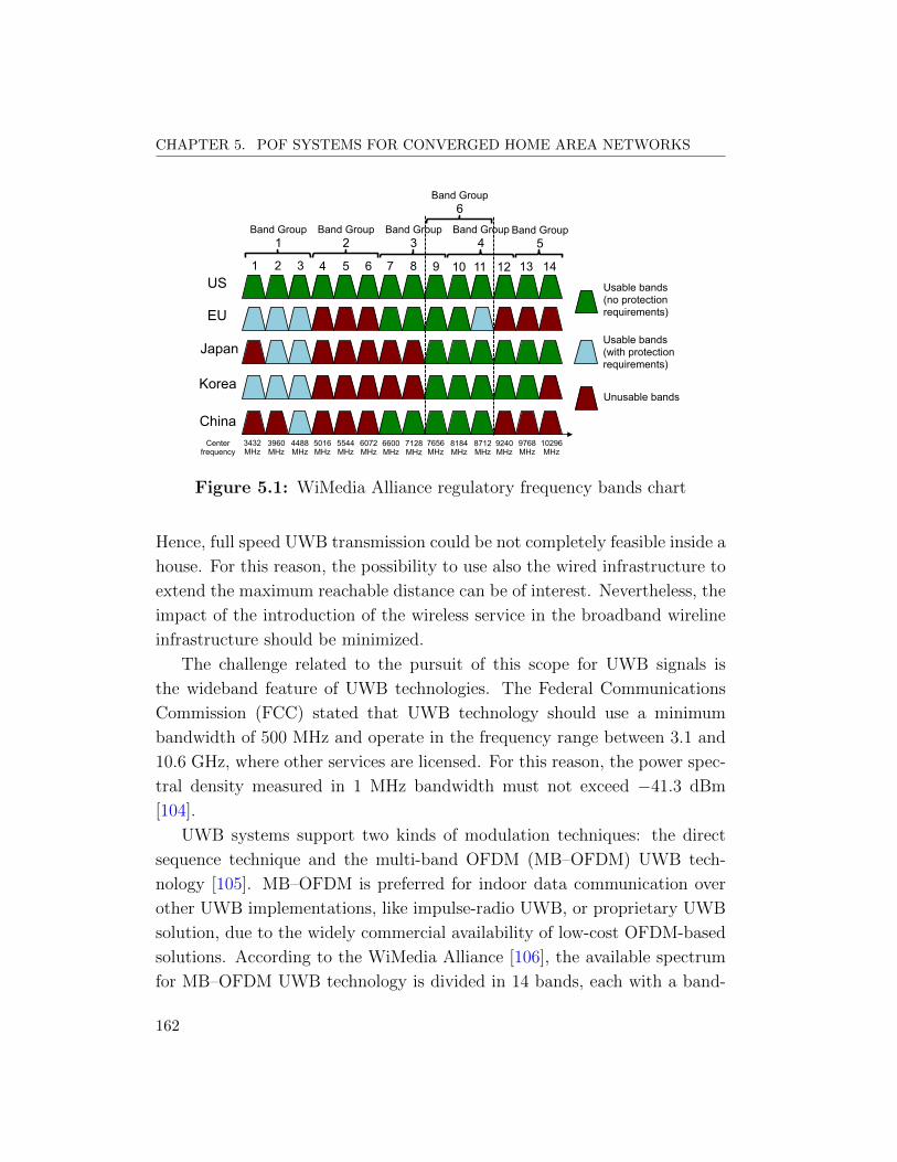
CHAPTER 5. POF SYSTEMS FOR CONVERGED HOME AREA NETWORKS
1 2 3 4 5 6 7 8 9 10 11 12 13 14
Band Group 1
Band Group 2
Band Group 5
Band Group 6
Band Group 3
Band Group 4
Usable bands (no protection requirements)
Usable bands (with protection requirements)
Unusable bands
US
EU
Japan
Korea
China Center
frequency 3432 MHz
3960 MHz
4488 MHz
5016 MHz
5544 MHz
6072 MHz
6600 MHz
7128 MHz
7656 MHz
8184 MHz
8712 MHz
9240 MHz
9768 MHz
10296 MHz
Figure 5.1: WiMedia Alliance regulatory frequency bands chart
Hence, full speed UWB transmission could be not completely feasible inside a
house. For this reason, the possibility to use also the wired infrastructure to
extend the maximum reachable distance can be of interest. Nevertheless, the
impact of the introduction of the wireless service in the broadband wireline
infrastructure should be minimized.
The challenge related to the pursuit of this scope for UWB signals is
the wideband feature of UWB technologies. The Federal Communications
Commission (FCC) stated that UWB technology should use a minimum
bandwidth of 500 MHz and operate in the frequency range between 3.1 and
10.6 GHz, where other services are licensed. For this reason, the power spec-
tral density measured in 1 MHz bandwidth must not exceed −41.3 dBm
[104].
UWB systems support two kinds of modulation techniques: the direct
sequence technique and the multi-band OFDM (MB–OFDM) UWB tech-
nology [105]. MB–OFDM is preferred for indoor data communication over
other UWB implementations, like impulse-radio UWB, or proprietary UWB
solution, due to the widely commercial availability of low-cost OFDM-based
solutions. According to the WiMedia Alliance [106], the available spectrum
for MB–OFDM UWB technology is divided in 14 bands, each with a band-
162

5.2. CONVERGED TRANSMISSION OF BASEBAND DMT AND UWB SIGNALS
width of 528 MHz as summarized in Fig 5.1. The first 12 bands are grouped
into 4 band groups counting 3 frequency bands each. The last two bands are
grouped in a fifth group. A sixth band group intended for worldwide usage
is also defined within the spectrum of the first four group bands.
The radio signal is based on an OFDM modulation format with 128 sub-
carriers, spaced by 4.125 MHz. A total of 110 subcarriers (100 data carriers
and 10 guard carriers) are used per band to transmit the information. Other
12 pilot subcarriers allow for coherent detection, while other 6 subcarriers,
including the one corresponding to the central frequency, are null. Hence,
122 subcarriers are used in total for each band. Frequency-domain spreading,
time-domain spreading, and FEC coding are provided for optimum perfor-
mance under a variety of channel conditions. The supported data rate ranges
from 53.3 to 480 Mbit/s [107]. For use within wireless USB technology the
support of transmitting and receiving data rate of 53.3, 106.7 and 200 Mbit/s
are mandatory within a maximum distance of 10 m, while the remaining data
rates up to 480 Mbit/s are optional [108].
5.2 Converged transmission of baseband DMT
and UWB signals
5.2.1 Experimental setup
The experimental setup used in our study is depicted in Fig. 5.2. A
Tektronix AWG7122 was used to generate the DMT signal in the same way
described in section 4.2.2. The real-time MB–OFDM UWB signal was gener-
ated by a Wisair development kit DV9110M. The UWB signal was centered
at 3.96 MHz and had a bandwidth of 528 MHz transporting 200 Mbit/s.
This bit-rate was imposed by the limitation of the particular UWB device,
but the concept is scalable to the full UWB data rate of 480 Mbit/s.
The POF link was the same described in section 4.2.2. The transmitter
was a red VCSEL with a peak optical power of 1 mW. The fiber was a 50 m
GI–POF with a core diameter of 1 mm. The receiver based on APD was
163
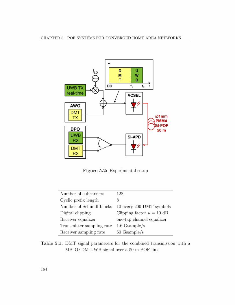
CHAPTER 5. POF SYSTEMS FOR CONVERGED HOME AREA NETWORKS
VCSEL
∅∅∅∅1mm
PMMA
GI-POF
50 m
DMTTX
AWG
DPO
UWBRX
UWB TXreal-time
Si-APD
DMTRX
U
W
B
D
M
T
f1 f2 f
fLO
DC
Figure 5.2: Experimental setup
Number of subcarriers 128
Cyclic prefix length 8
Number of Schimdl blocks 10 every 200 DMT symbols
Digital clipping Clipping factor µ = 10 dB
Receiver equalizer one-tap channel equalizer
Transmitter sampling rate 1.6 Gsample/s
Receiver sampling rate 50 Gsample/s
Table 5.1: DMT signal parameters for the combined transmission with a
MB–OFDM UWB signal over a 50 m POF link
164

5.2. CONVERGED TRANSMISSION OF BASEBAND DMT AND UWB SIGNALS
employed. The choice of the APD receiver is based on two considerations.
First, the 3 dB bandwidth of the link employing APD is higher than the 3 dB
bandwidth of the link employing PIN–PD. In second place, the frequency
response of the link employing APD is very flat within the 3 dB bandwidth.
Both features can be verified from Fig. 4.8 of chapter 4.
Due to the high center frequency of the UWB signal compared to the
3 dB bandwidth of the POF link, i.e. 1.31 GHz, the UWB signal was down-
converted to an intermediate frequency (IF). The DMT and UWB signals
were transported over the POF link splitting the available bandwidth into
two parts, DC to f1 for DMT and f1 to f2 for UWB, as summarized in
the inset in Fig. 5.2. In particular, the UWB signal was down-converted to a
center frequency of 1.1 GHz using an electrical mixer. Then, it was combined
with a low-pass DMT signal occupying the bandwidth below 0.8 GHz.
The DMT signal parameters are listed in Tab. 5.1. In particular, 128
subcarriers spaced by 6.25 MHz within the fixed bandwidth of 0.8 GHz were
used. To this purpose, the sampling rate of the AWG was fixed at 1.6 Gsam-
ple/s.
The electrical combination of DMT and down-converted UWB signals
were transmitted on the POF link. At the receiver side a real-time Tektronix
DPO72004 DPO was used to separately analyze the DMT and the UWB
performance. The quality of the UWB signal will be presented in terms of
EVM of the received quadrature phase shift keying (QPSK) constellation,
while for the DMT signal the maximum bit-rate achievable with a bit-error
rate below 10−3 will be considered, as done also for the experimental results
of chapter 4.
5.2.2 Experimental results and discussion
In Fig. 5.3 the power spectral density (PSD) of the transmitted (a) and
received (b) electrical combination of DMT and UWB signals is depicted. As
can be evinced from the figure, the DMT signal occupies the bandwidth below
0.8 GHz, while the UWB signal is allocated between 0.8 GHz and 1.4 GHz.
Note that both signals are not particularly distorted by the POF link, but
165

CHAPTER 5. POF SYSTEMS FOR CONVERGED HOME AREA NETWORKS
0 0.2 0.4 0.6 0.8 1 1.2 1.4
0
−10
−20
−30
−40
Frequency (GHz)
Nor
mal
ized
PS
D (
dBm
)
DMT UWB
(a) Transmitted PSD
0 0.2 0.4 0.6 0.8 1 1.2 1.4
0
−10
−20
−30
−40
Frequency (GHz)
Nor
mal
ized
PS
D (
dBm
)
DMT UWB
(b) Received PSD
Figure 5.3: Transmitted (a) and received (b) PSD for the combined trans-
mission of DMT and UWB signals
166
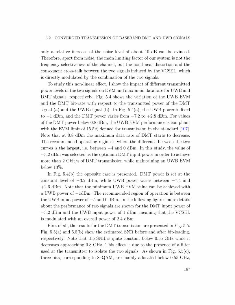
5.2. CONVERGED TRANSMISSION OF BASEBAND DMT AND UWB SIGNALS
only a relative increase of the noise level of about 10 dB can be evinced.
Therefore, apart from noise, the main limiting factor of our system is not the
frequency selectiveness of the channel, but the non linear distortion and the
consequent cross-talk between the two signals induced by the VCSEL, which
is directly modulated by the combination of the two signals.
To study this non-linear effect, I show the impact of different transmitted
power levels of the two signals on EVM and maximum data rate for UWB and
DMT signals, respectively. Fig. 5.4 shows the variation of the UWB EVM
and the DMT bit-rate with respect to the transmitted power of the DMT
signal (a) and the UWB signal (b). In Fig. 5.4(a), the UWB power is fixed
to −1 dBm, and the DMT power varies from −7.2 to +2.8 dBm. For values
of the DMT power below 0.8 dBm, the UWB EVM performance is compliant
with the EVM limit of 15.5% defined for transmission in the standard [107].
Note that at 0.8 dBm the maximum data rate of DMT starts to decrease.
The recommended operating region is where the difference between the two
curves is the largest, i.e. between −4 and 0 dBm. In this study, the value of
−3.2 dBm was selected as the optimum DMT input power in order to achieve
more than 2 Gbit/s of DMT transmission while maintaining an UWB EVM
below 13%.
In Fig. 5.4(b) the opposite case is presented. DMT power is set at the
constant level of −3.2 dBm, while UWB power varies between −7.4 and
+2.6 dBm. Note that the minimum UWB EVM value can be achieved with
a UWB power of −1dBm. The recommended region of operation is between
the UWB input power of −5 and 0 dBm. In the following figures more details
about the performance of two signals are shown for the DMT input power of
−3.2 dBm and the UWB input power of 1 dBm, meaning that the VCSEL
is modulated with an overall power of 2.4 dBm.
First of all, the results for the DMT transmission are presented in Fig. 5.5.
Fig. 5.5(a) and 5.5(b) show the estimated SNR before and after bit-loading,
respectively. Note that the SNR is quite constant below 0.55 GHz while it
decreases approaching 0.8 GHz. This effect is due to the presence of a filter
used at the transmitter to isolate the two signals. As shown in Fig. 5.5(c),
three bits, corresponding to 8–QAM, are mainly allocated below 0.55 GHz,
167
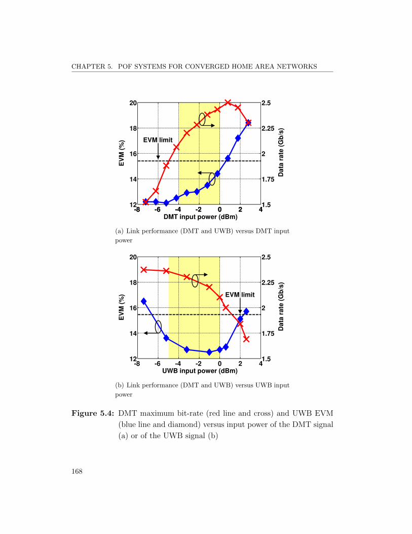
CHAPTER 5. POF SYSTEMS FOR CONVERGED HOME AREA NETWORKS
-8 -6 -4 -2 0 2 412
14
16
18
20
EV
M (
%)
-8 -6 -4 -2 0 2 41.5
1.75
2
2.25
2.5
DMT input power (dBm)
Da
ta r
ate
(G
b/s
)
EVM limit
(a) Link performance (DMT and UWB) versus DMT input
power
-8 -6 -4 -2 0 2 412
14
16
18
20
EV
M (
%)
UWB input power (dBm)
1.5
1.75
2
2.25
2.5
Da
ta r
ate
(G
b/s
)
EVM limit
(b) Link performance (DMT and UWB) versus UWB input
power
Figure 5.4: DMT maximum bit-rate (red line and cross) and UWB EVM
(blue line and diamond) versus input power of the DMT signal
(a) or of the UWB signal (b)
168

5.2. CONVERGED TRANSMISSION OF BASEBAND DMT AND UWB SIGNALS
0 0.4 0.80
4
8
12
16
Frequency (GHz)
SN
R (
dB
)
0 32 64 96 128subcarrier number
(a) SNR before bit-loading
0 0.2 0.4 0.6 0.80
4
8
12
16
Frequency (GHz)
SN
R (
dB
)
0 32 64 96 128subcarrier number
(b) SNR before bit-loading
0 0.2 0.4 0.6 0.80
1
2
3
4
Frequency (GHz)
Bit
allo
cati
on
(b
its)
0 32 64 96 128subcarrier number
(c) Bit allocation
0 0.2 0.4 0.6 0.8−3
−2
−1
0
1
2
3
Frequency (GHz)
Ene
rgy
dist
ribut
ion
(dB
)
0 32 64 96 128subcarrier number
(d) Power allocation
Figure 5.5: DMT bit loading application on the simultaneous transmission
of DMT and UWB signals over 50 m GI–POF : estimated SNR
before bit-loading (a), estimated SNR after bit-loading (b), bit
(c) and power (d) allocation
169
CHAPTER 5. POF SYSTEMS FOR CONVERGED HOME AREA NETWORKS
while two bits, corresponding to 4–QAM, are allocated above. The related
energy distribution is shown in Fig. 5.5(d). An almost constant value of
energy per subcarrier is allocated below 0.55 GHz, while increasing amounts
of energy per subcarrier are allocated between 0.55 and 0.8 GHz. In this way
the SNR after bit-loading assumes mainly two values corresponding to the
allocated bits as depicted in Fig. 5.5(b).
0 0.2 0.4 0.6 0.81E−4
1E−3
1E−2
Frequency (GHz)
BE
R p
er s
ubca
rrie
r
0 32 64 96 128subcarrier number
Total BER
(a) (b)
Figure 5.6: DMT BER performance per subcarrier (a) and constellation
diagram of the demodulated signal for the subcarriers with 8–
QAM (b)
With the optimum bit and power allocation a gross bit-rate of 2.2 Gbit/s
was achieved with a BER of 8.5 × 10⁻⁴, which is below the target of 10−3.
Fig. 5.6(a) shows the measured BER per subcarrier. The BER of the sub-
carriers is mainly below the overall BER, and just few subcarriers are above
the target BER of 10−3. Fig. 5.6(b) shows the superimposed equalized con-
stellation diagram of all the subcarriers with 8–QAM, corresponding to three
allocated bits.
Accounting for cyclic prefix and Schimdl blocks within the gross bit-rate
of 2.2 Gbit/s, the uncoded net bit-rate is 2 Gbit/s, corresponding to a spec-
tral efficiency of 2.5 bit/s/Hz. Accounting also for a 6.7% EFEC overhead,
the net bit-rate for error-free operation becomes 1.9 Gbit/s. Hence, gigabit
170

5.2. CONVERGED TRANSMISSION OF BASEBAND DMT AND UWB SIGNALS
transmission is well supported with this scheme.
0 100 200 Time (µs)
Volta
ge (a
.u.)
150 50
(a)
-‐20
-‐30
-‐40
-‐50
-‐60
-‐70
3168 3432 3696 3960 4224 4488 4752
Power (d
Bm)
Frequency (MHz)
ACPR21: 34.67 dB PASS ACPR23: 34.10 dB PASS
Spectral Mask: PASS
-23.4 dBm
5MHz RBW
(b)
Figure 5.7: Time (a) and spectrum (b) behaviors of the received up-
converted UWB signal
I show now the results related to UWB transmission. These results are
determined on the off-line up-converted UWB signal. Indeed, the received
UWB signal at the IF of 1.1 GHz was at first digitally converted by the DPO.
Then, to analyze this signal with a Tektronix proprietary MB–OFDM analy-
sis software, an off-line filtering and up-conversion was performed. Fig. 5.7(a)
shows the time behavior of the received MB–OFDM signal, where the frame
structure can be observed. Fig. 5.7(b) shows instead the spectral mask anal-
171
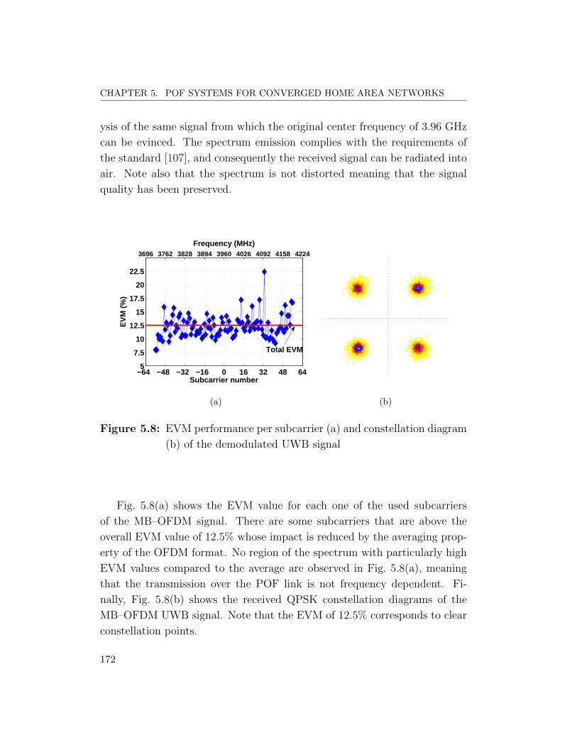
CHAPTER 5. POF SYSTEMS FOR CONVERGED HOME AREA NETWORKS
ysis of the same signal from which the original center frequency of 3.96 GHz
can be evinced. The spectrum emission complies with the requirements of
the standard [107], and consequently the received signal can be radiated into
air. Note also that the spectrum is not distorted meaning that the signal
quality has been preserved.
−64 −48 −32 −16 0 16 32 48 645
7.5
10
12.5
15
17.5
20
22.5
Subcarrier number
EV
M (
%)
3696 3762 3828 3894 3960 4026 4092 4158 4224
Frequency (MHz)
Total EVM
(a) (b)
Figure 5.8: EVM performance per subcarrier (a) and constellation diagram
(b) of the demodulated UWB signal
Fig. 5.8(a) shows the EVM value for each one of the used subcarriers
of the MB–OFDM signal. There are some subcarriers that are above the
overall EVM value of 12.5% whose impact is reduced by the averaging prop-
erty of the OFDM format. No region of the spectrum with particularly high
EVM values compared to the average are observed in Fig. 5.8(a), meaning
that the transmission over the POF link is not frequency dependent. Fi-
nally, Fig. 5.8(b) shows the received QPSK constellation diagrams of the
MB–OFDM UWB signal. Note that the EVM of 12.5% corresponds to clear
constellation points.
172
5.3. SUMMARY
5.3 Summary
The experimental verification of a converged infrastructure based on large
core PMMA POF for the transmission of broadband wired and wireless ser-
vices has been presented in this chapter. After a short introduction on the
MB–OFDM UWB wireless technology used in this activity in section 5.1, the
simultaneous transmission over 50 m GI-POF of DMT and UWB signals has
been investigated in section 5.2.
An experimental study on the impact of the non-linearity of the laser
source was performed to determine the optimum signal power values for
transmission. An uncoded net bit-rate of 2 Gbit/s with BER< 10−3 was
obtained with DMT transmission and bit-loading. A 528 MHz WiMedia-
compliant UWB signal transporting 200 Mbit/s was successfully demon-
strated on the link guaranteing an EVM of 12.5% on the received QPSK
constellation.
173

CHAPTER 5. POF SYSTEMS FOR CONVERGED HOME AREA NETWORKS
174
Conclusions
This thesis dealt with fiber-optic technologies enabling an efficient dis-
tribution of broadband wireline and wireless communication services for in-
building networks. An overview of silica fibers and 1 mm core diameter
PMMA plastic optical fibers has been addressed in chapter 1. Silica fiber
is recognized as the more appropriate fiber medium for large and medium
in-building networks. At present, OM laser-optimized multimode fibers can
guarantee 10 Gbit/s transmission up to 550 m, and 40 or 100 Gbit/s up
to 150 m. If distance or data rate increases, singlemode fiber becomes the
most appropriate medium. In accordance with these considerations, fiber
distributed antenna systems based on single and multimode fibers were intro-
duced as an enabling technology to provide wireless coverage and high data
rate with current and emerging wireless technologies in large and medium
buildings. Radio over fiber systems employing intensity modulated - direct
detection were considered as cost-effective solutions to realize F–DASs in an
in-building scenario.
The major cost-sensitivity of small building networks with respect to large
and medium building networks was pointed out. For this scenario, PMMA
plastic optical fibers with a core diameter of approximately 1 mm were dis-
cussed as an alternative to copper solutions, such as Cat-5. The feasibility
of an in-building optical backbone employing plastic optical fibers has been
related to the possibility of multi-gigabit transmission and the capability to
transport wireless services.
175

CONCLUSIONS
Wireline
Wireless
SMF
Modeling of state-‐of-‐the-‐art IM-‐DD links with directly modulated DFBs. UMTS and WiMAX signals transmission experiments
(Chapter 2)
MMF
Design and opFmizaFon of an IM-‐DD RoMMF link up to 525 m with: worst-‐case SFDR exceeding 105 dB×Hz2/3 worst-‐case LTE-‐ACLR below -‐48 dBc
(Chapter 3)
POF
Record transmission on 50 m GI-‐POF with DMT and 2N + 3×2N -‐QAM formats of: 5.4 Gbit/s with APD 5.15 Gbit/s with PIN-‐PD
(Chapter 4)
Converged transport on 50 m GI-‐POF link with APD of: 2 Gbit/s with DMT 200 Mbit/s with MB-‐OFDM UWB
(Chapter 5)
Fiber
Service
Large and medium
buildings S
mall buildings
Figure 1: Summary of the main technical achievements of this thesis
Fig. 1 summarizes the main technical achievements of this work.
Chapter 2 dealt with IM–DD RoF links with directly modulated DFBs
for wireless signal distribution on singlemode fiber. A modeling tool was
developed to describe in an accurate and efficient way the simultaneous
transmission of radio signals. The experimental activity pointed out the
interactions between two modulating RF signals compliant with UMTS and
WiMAX standards. A good agreement between experimental and simulation
results has been reported. The wide feasibility of IM–DD RoF links over few
kilometers of single mode fibers has been verified, while some criticalities
have been underlined for longer links due to identified linear and non-linear
characteristics of the laser.
Chapter 3 reported my research activity on IM–DD RoF links with di-
rectly modulated lasers for wireless signal distribution on multimode fiber.
The comprehensive theoretical and experimental research has clarified the
physical mechanisms of the main transmission impairments of IM–DD
RoMMF systems, and allowed to develop design guidelines for enhancing
the performance. The main detrimental effect in short-range RoMMF links
176
CONCLUSIONS
is modal noise which leads to a time fluctuation of the link gain and to an
increment of distortion effects. These undesired effects have been proved to
be strictly related to the launching condition, the photodiode structure and
the source characteristics, such as frequency chirping and non-linearity. The
impact of modal noise can be adequately controlled when a central launch,
as opposed to offset and overfilled launches, is applied, a photodiode with a
built-in ball lens is used, and a Fabry-Perot laser with low frequency chirp-
ing, high modulation efficiency, and non-linearity properties comparable with
DFBs is employed. With the designed link a worst-case SFDR exceeding
105 dB× Hz2/3 up to 525 m was obtained. Hence, a successful transmission
of LTE signals in a dual-band configuration was verified giving worst-case
ACLR performance below −48 dBc at 525 m.
Chapter 4 showed my activity on 1 mm core diameter POF systems
for high-speed wireline transmission in small buildings and home networks.
Closed-form equations for the modeling of the channel capacity of POF links
has been derived describing the complete transmission chain with super-
gaussian functions. Multi-gigabit transmission experiments over 1 mm core
diameter PMMA GI–POF were performed employing simple and eye–safety
compliant VCSEL transmitter and two photoreceivers, one based on a 230 µm
active-area diameter Si–APD and another based on a 400 µm active-area
diameter Si–PIN PD. It has been shown that by using these simple com-
ponents in combination with DMT modulation and bit-loading, uncoded
net bit-rates of 4.85 and 5.15 Gbit/s with BER< 10−3 over 50 m POF are
achievable with APD and PIN–PD, respectively. These bit-rates are distant
0.75 and 0.25 Gbit/s, respectively, from the maximum achievable channel
capacity employing M–QAM. To approach even closely the channel capac-
ity, 3×2N–QAM constellations, corresponding to a fractional number of bits
per symbol, were added to the constellation set used for the data rate op-
timization within the DMT bit-loading algorithm. This led to an half-bit
granularity in the bit-loading algorithm, enabling a potential higher spectral
efficiency in the use of the channel. With this new scheme the uncoded net
bit-rate of the system employing APD becomes 5.4 Gbit/s keeping a distance
of only 0.2 Gbit/s from the maximum achievable capacity with M–QAM.
177
CONCLUSIONS
Chapter 5 depicted my work on wireless and wireline signal distribution
on 1 mm core diameter POF systems intended for short-range communica-
tions inside a small building and a home network. An experimental feasibility
study of a simultaneous transmission on a single 1 mm core diameter POF of
a UWB radio signal and a baseband data stream was performed. An uncoded
net bit-rate of 2 Gbit/s with BER< 10−3 was achieved after 50 m transmis-
sion employing DMT modulation with bit-loading. A 528 MHz WiMedia-
compliant UWB signal transporting 200 Mbit/s was successfully transported
on the link leading to an EVM of 12.5% on the received QPSK constellation,
which is better than the maximum required EVM.
As mentioned in the Introduction, the aim of this thesis was to investigate
the convenience and necessity of fiber-optic technologies for in-building net-
works now that wireless technologies are driving the market. Some answers
can be found in the work presented in this thesis:
• Different fiber-optic technologies (SMF, MMF and POF) are convenient
for different in-building scenarios (large, medium and small buildings)
• Intensity modulation and direct detection systems are the most at-
tractive solutions for present and near-future short-range fiber-optic
systems
• Advanced digital modulation formats can counterpoise the intrinsic
limitations of fiber-optic technologies different from SMF (in this thesis
it was shown for POF systems)
• A positive mutual cooperation is possible between fiber-optic and wire-
less technologies. For large and medium buildings a dedicated fiber
distributed antenna system on SMF and/or MMF can answer for the
multi-operator, multi-service needs. For small buildings, including
home scenarios, a converged wireline and wireless optical backbone
has to be considered (in this thesis it was shown with a POF system)
Further research activities are needed to study the ultimate capacity lim-
its of fiber-optic solutions different from SMF. Moreover, this thesis dealt
178

CONCLUSIONS
with point-to-point links, while also the impact of a complete network ar-
chitecture needs to be considered. More generally, in a strategic future per-
spective, an appropriate converged wireline and wireless optical infrastruc-
ture appears to be the solution to transport and manage all the potential
in-building services also in large and medium buildings. This will be a direc-
tion to which research bodies and private industries will have to direct their
investigation activities.
179

CONCLUSIONS
180
Bibliography
[1] B. Skutnik and C. Smith, “Multimode, Large-Core and Plastic Clad
(PCS) Fibers,” in Specialty Optical Fibers Handbook, A. Mendez and
T. Morse, Eds. Oxford: Academic Press, 2007.
[2] A. Bjarklev, A. Bjarklev, and J. Broeng, Photonic crystal fibers. New
York: Springer, 2003.
[3] G. Agrawal, Fiber-Optic Communication Systems, 3rd ed. New York:
Wiley, 2002.
[4] Characteristics of a single-mode optical fiber cable, ITU-T Recommen-
dation G.652, 2009.
[5] “Corning SMF-28e+ optical fiber with nexcor technology product in-
formation,” Corning Incorporated, Corning, NY.
[6] B. Saleh and M. Teich, Fundamentals of Photonics,. New York: Wiley,
1991,.
[7] Characteristics of a 50/125 µm multimode graded index optical fibre
cable for the optical access network, ITU-T Recommendation G.651.1,
2007.
[8] Information technology - Generic cabling for customer premises,
ISO/IEC Std. 11 801, 2009.
181

BIBLIOGRAPHY
[9] P. Kish. (2010, Jan.) Next generation fibers ar-
rive. [Online]. Available: http://www.cnsmagazine.com/news/
next-generation-fiber-arrives/1000355010/
[10] J. Zubia and J. Arrue, “Plastic optical fibers: An introduction to their
technological processes and applications,” Optical Fiber Technology,
vol. 7, no. 2, pp. 101–140, Apr. 2001.
[11] O. Ziemann, J. Krauser, P. E. Zamzow, and W. Daum, POF Handbook:
Optical Short Range Transmission Systems, 2nd ed. Berlin: Springer-
Verlag, 2008.
[12] Optical fibre cables - Part 2-40: Indoor optical fibre cables - Family
specification for A4 fibre cables, IEC Std. 60 794-2-40, 2008.
[13] IEEE Standard for Information Technology - Telecommunications and
Information Exchange Between Systems - Local and Metropolitan Area
Networks - Specific Requirements. Part 3: Carrier Sense Multiple Ac-
cess With Collision Detection (CSMA/CD) Access Method and Physi-
cal Layer Specifications, IEEE Std. 802.3, 1998.
[14] IEEE Standard for Information Technology - Telecommunications and
Information Exchange Between Systems - Local and Metropolitan Area
Networks - Specific Requirements. Supplement to Carrier Sense Multi-
ple Access With Collision Detection (CSMA/CD) Access Method and
Physical Layer Specifications - Physical Layer Parameters and Specifi-
cations for 1000 Mb/s Operation Over 4-Pair of Category 5 Balanced
Copper Cabling, Type 1000BASE-T, IEEE Std. 802.3ab, 1999.
[15] IEEE Standard for Information Technology-Telecommunications and
Information Exchange Between Systems-Local and Metropolitan Area
Networks-Specific Requirements Part 3: Carrier Sense Multiple Ac-
cess With Collision Detection (CSMA/CD) Access Method and Physi-
cal Layer Specifications, IEEE Std. 802.3an, 2006.
182
BIBLIOGRAPHY
[16] A. Nespola, S. Straullu, P. Savio, D. Zeolla, S. Abrate, D. Cardenas,
J. Ramirez, N. Campione, and R. Gaudino, “First demonstration of
real-time LED-based gigabit ethernet transmission on 50m of A4a.2
SI-POF with significant system margin,” in 36th European Conference
on Optical Communication (ECOC) 2010, Torino, Italy, 19–23 Sep.
2010, p. PD3.1.
[17] A. Antonino, S. Straullu, S. Abrate, A. Nespola, P. Savio, D. Zeolla,
J. R. Molina, R. Gaudino, S. Loquai, and J. Vinogradov, “Real-time
gigabit ethernet bidirectional transmission over a single SI-POF up to
75 meters,” in Conference on Optical Fiber Communication/National
Fiber Optic Engineers Conference (OFC/NFOEC) 2011, Los Angeles,
CA, 6–10 Mar. 2011, p. OWA2.
[18] H. Yang, E. Tangdiongga, S. C. J. Lee, C. M. Okonkwo, H. P. A.
van den Boom, S. Randel, and A. M. J. Koonen, “4.7 Gbit/s transmis-
sion over 50m long 1mm diameter multi-core plastic optical fiber,” in
Conference on Optical Fiber Communication/National Fiber Optic En-
gineers Conference (OFC/NFOEC) 2010, San Diego, CA, 21–25 Mar.
2010, p. OWA4.
[19] D. O’Brien, L. Zeng, H. Le-Minh, G. Faulkner, O. Bouchet, S. Randel,
J. Walewski, J. Rabadan Borges, K.-D. Langer, J. Grubor, K. Lee, and
E. Tae Won, “Visible light communications,” in Short-Range Wireless
Communications: Emerging Technologies and Applications, R. Krae-
mer and M. Katz, Eds. Chichester: Wiley, 2009.
[20] J. Kahn and J. Barry, “Wireless infrared communications,” Proceedings
of the IEEE, vol. 85, no. 2, pp. 265–298, Feb. 1997.
[21] IEEE 802.11TMWIRELESS LOCAL AREA NETWORKS; the
working group for wlan standards. [Online]. Available: http:
//www.ieee802.org/11/
183

BIBLIOGRAPHY
[22] Evolved Universal Terrestrial Radio Access (E-UTRA); Base Station
(BS) radio transmission and reception, 3GPP Technical Specification
36.141 Release 8, V8.12.0, 2011.
[23] (2010, Oct.) ITU paves way for next-generation 4G mobile
technologies. [Online]. Available: http://www.itu.int/net/pressoffice/
press releases/2010/40.aspx/
[24] M. Fabbri and P. Faccin, “Radio over fiber technologies and sys-
tems: New opportunities,” in 9th International Conference on Trans-
parent Optical Networks (ICTON) 2007, Rome, Italy, 1–5 Jul. 2007, p.
We.C3.1.
[25] J. Capmany and D. Novak, “Microwave photonics combines two
worlds,” Nature Photonics, vol. 1, no. 6, pp. 319–330, Jun. 2007.
[26] I. Cox, C.H., E. Ackerman, G. Betts, and J. Prince, “Limits on the
performance of RF-over-fiber links and their impact on device design,”
IEEE Transactions on Microwave Theory and Techniques, vol. 54,
no. 2, pp. 906–920, Feb. 2006.
[27] T. Kurniawan, A. Nirmalathas, C. Lim, D. Novak, and R. Waterhouse,
“Performance analysis of optimized millimiter-wave fiber radio lilnks,”
IEEE/OSA Journal of Lightwave Technology, vol. 54, no. 2, pp. 921–
928, Feb. 2006.
[28] M. Beltran, J. Jensen, R. Llorente, and I. Tafur Monroy, “Experi-
mental analysis of 60-GHz VCSEL and ECL photonic generation and
transmission of impulse-radio ultra-wideband signals,” IEEE Photonics
Technology Letters, vol. 23, no. 15, pp. 1055–1057, Aug. 2011.
[29] C.-S. Choi, J.-H. Seo, W.-Y. Choi, H. Kamitsuna, M. Ida, and
K. Kurishima, “60-GHz bidirectional radio-on-fiber links based on InP-
InGaAs HPT optoelectronic mixers,” IEEE Photonics Technology Let-
ters, vol. 17, no. 12, pp. 2721–2723, Dec. 2005.
184

BIBLIOGRAPHY
[30] D. Zibar, R. Sambaraju, A. Caballero, J. Herrera, U. Westergren,
A. Walber, J. Jensen, J. Marti, and I. Monroy, “High-capacity wireless
signal generation and demodulation in 75- to 110-GHz band employ-
ing all-optical OFDM,” IEEE Photonics Technology Letters, vol. 23,
no. 12, pp. 810–812, Jun. 2011.
[31] P. Gamage, A. Nirmalathas, C. Lim, D. Novak, and R. Waterhouse,
“Design and analysis of digitized RF-over-fiber links,” IEEE/OSA
Journal of Lightwave Technology, vol. 27, no. 12, pp. 2052–2061, Jun.
2009.
[32] D. Wake, A. Nkansah, and N. J. Gomes, “Radio over fiber link design
for next generation wireless systems,” IEEE/OSA Journal of Lightwave
Technology, vol. 28, no. 16, pp. 2456–2464, Aug. 2010.
[33] I. Cox, C.H., G. Betts, and L. Johnson, “An analytic and experi-
mental comparison of direct and external modulation in analog fiber-
optic links,” IEEE Transactions on Microwave Theory and Techniques,
vol. 38, no. 5, pp. 501–509, May 1990.
[34] I. Cox, C., E. Ackerman, R. Helkey, and G. Betts, “Direct-detection
analog optical links,” IEEE Transactions on Microwave Theory and
Techniques, vol. 45, no. 8, pp. 1375–1383, Aug. 1997.
[35] N. J. Gomes, A. Nkansah, and D. Wake, “Radio-over-MMF techniques
- part I: RF to microwave frequency systems,” IEEE/OSA Journal of
Lightwave Technology, vol. 26, no. 15, pp. 2388–2395, Aug. 2008.
[36] H. Al-Raweshidy and S. Komaki, Radio Over Fiber Technologies for
Mobile Communication Networks. Boston: Artech House, 2002.
[37] A. Nkansah and N. J. Gomes, “Characterization of radio over multi-
mode fiber links using coherence bandwidth,” IEEE Photonics Tech-
nology Letters, vol. 17, no. 12, pp. 2694–2696, Dec. 2005.
[38] G. Tartarini and P. Faccin, “Efficient characterization of harmonic and
intermodulation distortion effects in dispersive radio over fiber systems
185
BIBLIOGRAPHY
with direct laser modulation,” Microwave and Optical Technology Let-
ters, vol. 46, no. 2, pp. 114–117, Jul. 2005.
[39] R. Kalman, J. Fan, and L. Kazovsky, “Dynamic range of coherent
analog fiber-optic links,” IEEE/OSA Journal of Lightwave Technology,
vol. 12, no. 7, pp. 1263–1277, Jul. 1994.
[40] R. Taylor and S. Forrest, “Optically coherent direct modulated FM
analog link with phase noise canceling circuit,” IEEE/OSA Journal of
Lightwave Technology, vol. 17, no. 4, pp. 556–563, apr 1999.
[41] N. Walker, D. Wake, and I. Smith, “Efficient millimetre-wave signal
generation through FM-IM conversion in dispersive optical fibre links,”
Electronics Letters, vol. 28, no. 21, pp. 2027–2028, Oct. 1992.
[42] T. Darcie, J. Zhang, P. Driessen, and J.-J. Eun, “Class-B microwave-
photonic link using optical frequency modulation and linear frequency
discriminators,” IEEE/OSA Journal of Lightwave Technology, vol. 25,
no. 1, pp. 157–164, Jan. 2007.
[43] G. Chen, J. Kang, and J. Khurgin, “Frequency discriminator based on
ring-assisted fiber sagnac filter,” IEEE Photonics Technology Letters,
vol. 17, no. 1, pp. 109–111, Jan. 2005.
[44] V. Urick, F. Bucholtz, J. McKinney, P. Devgan, A. Campillo, J. Dexter,
and K. Williams, “Long-haul analog photonics,” IEEE/OSA Journal
of Lightwave Technology, vol. 29, no. 8, pp. 1182–1205, Apr. 2011.
[45] M. LaGasse and S. Thaniyavaru, “Bias-free high-dynamic-range phase-
modulated fiber-optic link,” IEEE Photonics Technology Letters, vol. 9,
no. 5, pp. 681–683, May 1997.
[46] B. Davies and J. Conradi, “Hybrid modulator structures for subcar-
rier and harmonic subcarrier optical single sideband,” IEEE Photonics
Technology Letters, vol. 10, no. 4, pp. 600–602, Apr. 1998.
186

BIBLIOGRAPHY
[47] H. Kim, “Integrated transmitter with amplitude and phase modula-
tions,” in IEEE PhotonicsGlobal@Singapore (IPGC) 2008, Singapore,
8–11 Dec. 2008.
[48] U.-S. Lee, H.-D. Jung, and S.-K. Han, “Optical single sideband signal
generation using phase modulation of semiconductor optical amplifier,”
IEEE Photonics Technology Letters, vol. 16, no. 5, pp. 1373–1375, May
2004.
[49] The nano3GTMaccess points. [Online]. Available: http://www.
ipaccess.com/en/nano3G-access-point/
[50] H. Yang, Y. Shi, W. Wang, C. M. Okonkwo, H. P. A. van den Boom,
A. M. J. Koonen, and E. Tangdiongga, “Wimedia-compliant UWB
transmission over 1 mm core diameter plastic optical fibre,” IET Elec-
tronics Letters, vol. 46, no. 6, pp. 434–436, Mar. 2010.
[51] T. D. Michaelis, “Laser diode evaluation for optical analog link,” IEEE
Transactions on Cable Television, vol. CATV-4, no. 1, pp. 30–42, Jan.
1979.
[52] J. L. Prince, E. I. Ackerman, and I. Cox, C. H., “Analog fiber-optic
link technology,” in Digest of the LEOS Summer Topical Meetings on
Biophotonics/Optical Interconnects and VLSI Photonics/WBM Micro-
cavities 2004, Jun. 2004.
[53] A. Villafranca, J. Lasobras, and I. Garces, “Precise characterization
of the frequency chirp in directly modulated DFB lasers,” in Spanish
Conference on Electron Devices (CDE) 2007, Madrid, Spain, Jan. 31-
Feb. 2 2007, pp. 173–176.
[54] R. Chan and J. Liu, “Time-domain wave propagation in optical struc-
tures,” IEEE Photonics Technology Letters, vol. 6, no. 8, pp. 1001–
1003, Aug. 1994.
187
BIBLIOGRAPHY
[55] S. Ryu and S. Yamamoto, “Measurement of direct frequency modula-
tion characteristics of DFB-LD by delayed self-homodyne technique,”
IET Electronics Letters, vol. 22, no. 20, pp. 1052–1054, Sep. 1986.
[56] U. Kruger and K. Kruger, “Simultaneous measurement of the
linewidth, linewidth enhancement factor α, and FM and AM response
of a semiconductor laser,” IEEE/OSA Journal of Lightwave Technol-
ogy, vol. 13, no. 4, pp. 529–597, Apr. 1995.
[57] A. Yariv and P. Yeh, Photonics: Optical Electronics in Modern Com-
munications, 6th ed. New York, Oxford: Oxford Universirt Press,
2006.
[58] Telecommunications: Glossary of Telecommunication Terms, General
Services Administration Federal Standard 1037C, 1996.
[59] M. Abramowitz and I. Stegun, Handbook of Mathematical Functions
with Formulas, Graphs, and Mathematical Tables, 10th ed. Washing-
ton: National Bureau of Standardds, 1972.
[60] Universal Mobile Telecommunications System (UMTS); Base Station
(BS) radio transmission and reception (FDD), 3GPP Technical Speci-
fication 25.104 Release 8, V8.13.0, 2011.
[61] WiMAX Forum R© Air Interface Specifications; WiMAX Forum R© Mo-
bile Radio Specification, WiMAX Forum Technical Specification T23-
005-R015v04, 2010.
[62] Universal Mobile Telecommunications System (UMTS); User Equip-
ment (UE) radio transmission and reception (FDD), 3GPP Technical
Specification 25.101 Release 8, V8.15.0, 2011.
[63] S. Bottacchi, Multi-gigabit Transmission Over Multimode Optical Fi-
bre: Theory and Design Methods for 10GbE Systems. New York:
Wiley, 2006.
188

BIBLIOGRAPHY
[64] J. Fleming, “Dispersion in GeO2–SiO2 glasses,” OSA Appled Optics,
vol. 23, no. 24, pp. 4486–4493, Dec. 1984.
[65] D. Donlagic, “Opportunities to enhance multimode fiber links by ap-
plication of overfilled launch,” IEEE/OSA Journal of Lightwave Tech-
nology, vol. 23, no. 11, pp. 3526–3540, Nov. 2005.
[66] G. Tartarini and H. Renner, “Efficient finite-element analysis of tilted
open anisotropic optical channel waveguides,” IEEE Microwave and
Guided Wave Letters, vol. 9, no. 10, pp. 389–391, Oct. 1999.
[67] “RF module,” Model Library, COMSOL AB, Stockholm, Sweden, Nov.
2008.
[68] M. Ohashi, K. Kitayama, Y. Ishida, and Y. Negishi, “Simple approx-
imations for chromatic dispersion in single-mode fibers with various
index profiles,” IEEE/OSA Journal of Lightwave Technology, vol. 3,
no. 1, pp. 110–115, Feb. 1985.
[69] L. Raddatz, I. H. White, D. G. Cunningham, and M. C. Nowell, “An
experimental and theoretical study of the offset launch technique for the
enhancement of the bandwidth of multimode fiber links,” IEEE/OSA
Journal of Lightwave Technology, vol. 16, no. 3, pp. 324–331, Mar.
1998.
[70] L. Raddatz and I. H. White, “Overcoming the modal bandwidth limi-
tation of multimode fiber by using passband modulation,” IEEE Pho-
tonics Technology Letters, vol. 11, no. 2, pp. 266–268, Feb. 1999.
[71] L. Geng, C. Kwok, S. Lee, J. Ingham, R. Penty, I. White, and
D. Cunningham, “Efficient line launch for bandwidth improvement of
10 Gbit/s multimode fibre links using elliptical gaussian beam,” in
36th European Conference on Optical Communication (ECOC) 2009,
Torino, Italy, 19–23 Sep. 2010, p. We.6.B.5.
189

BIBLIOGRAPHY
[72] D. H. Sim, Y. Takushima, and Y. C. Chung, “High-speed multimode
fiber transmission by using mode-field matched center-launching tech-
nique,” IEEE/OSA Journal of Lightwave Technology, vol. 27, no. 8,
pp. 1018–1026, Apr. 2009.
[73] I. Gasulla and J. Capmany, “Transfer function of multimode fiber links
using an electric field propagation model: Application to radio over
fibre systems,” OSA Optics Express, vol. 14, no. 20, pp. 9051–9070,
Oct. 2006.
[74] J. Capmany and I. Gasulla, “Transfer function of radio over fiber multi-
mode fiber optic links considering third-order dispersion,” OSA Optics
Express, vol. 15, no. 17, pp. 10 591–10 596, Aug. 2007.
[75] B. Crosignani and A. Yariv, “Statistical properties of modal noise
in fiber-laser systems,” OSA Journal of Optical Society of America,
vol. 73, no. 8, pp. 1022–1027, Aug. 1983.
[76] G. Ghosh, M. Endo, and T. Iwasaki, “Temperature-dependent Sell-
meier coefficients and chromatic dispersions for some optical fiber
glasses,” IEEE/OSA Journal of Lightwave Technology, vol. 12, no. 8,
pp. 1338–1342, Aug. 1994.
[77] G. Ghosh and H. Yajima, “Pressure-dependent sellmeier coefficients
and material dispersions for silica fiber glass,” IEEE/OSA Journal of
Lightwave Technology, vol. 16, no. 11, pp. 2002–2005, Nov. 1998.
[78] R. Dandliker, A. Bertholds, and F. Maystre, “How modal noise in
multimode fibers depends on source spectrum and fiber dispersion,”
IEEE/OSA Journal of Lightwave Technology, vol. 3, no. 1, pp. 7–12,
Feb. 1985.
[79] I. Gasulla and J. Capmany, “Modal noise impact in radio over fiber
multimode fiber links,” OSA Optics Express, vol. 16, no. 1, pp. 121–
126, Jan. 2008.
190
BIBLIOGRAPHY
[80] “Mode conditiong patchcord IEC 61300,” Diamond SA, Losone,
Switzerland.
[81] “FM-1 mode scrambler,” Newport Corporation, Irvine, CA.
[82] Evolved Universal Terrestrial Radio Access (E-UTRA); Base Station
(BS) conformance testing, 3GPP Technical Specification 36.141 Re-
lease 8, V8.11.0, 2011.
[83] C. Shannon, “Communication in the presence of noise,” Proceedings of
the IRE, vol. 37, no. 1, pp. 10–21, Jan. 1949.
[84] T. M. Cover and J. A. Thomas, Elements of lnformation Theory,
2nd ed. New York: Wiley, 2006.
[85] G. Agrawal, Nonlinear Fiber Optics, 3rd ed. San Diego: Academic
Press, 2001.
[86] D. Cardenas, A. Nespola, P. Spalla, S. Abrate, and R. Gaudino, “A me-
dia converter prototype for 10-Mb/s Etherent transmission over 425 m
of large-core step-index polymer optical fiber,” IEEE/OSA Journal of
Lightwave Technology, vol. 24, no. 12, pp. 4946–4952, Dec. 2006.
[87] J. Bingham, “Multicarrier modulation for data transmission: an idea
whose time has come,” IEEE Communications Magazine, vol. 28, no. 5,
pp. 5–14, May 1990.
[88] S. Lee, “Discrete multitone modulation for short-range optical com-
muncations,” Ph.D. dissertation, Eindhoven University of Technology,
Dec. 2009.
[89] J. Cioffi. (2008) A multicarrier primer. [Online]. Available: http:
//www.stanford.edu/group/cioffi/documents/multicarrier.pdf
[90] D. Forney. (Spring 2005) Principles of digital commu-
nication II (lecture notes). [Online]. Available: http:
//ocw.mit.edu/courses/electrical-engineering-and-computer-science/
6-451-principles-of-digital-communication-ii-spring-2005/
191

BIBLIOGRAPHY
[91] Forward error correction for high-bit rate DWDM submarine systems,
ITU-T Recommendation G.975.1, 2004.
[92] P. S. Chow, J. M. Cioffi, and J. A. C. Bingham, “A practical dis-
crete multitone transceiver loading algorithm for data transmission over
spectrally shaped channels,” IEEE Transactions on Communications,
vol. 43, no. 234, pp. 773–775, Feb./Mar./Apr. 1995.
[93] J. Cioffi. (Spring Quarter 2007-2008) Advanced digital communication
(course handouts). [Online]. Available: http://www.stanford.edu/
class/ee379c/
[94] “665 nm multimode VCSEL (RVM665T) preliminary product specifi-
cation,” Firecomms Ltd., Cork, Ireland.
[95] Safety of laser products - Part 1: Equipment classification and require-
ments, IEC Std. 60 825-1, 2007.
[96] “OM-GIGA product specification,” Optimedia, Inc., Korea.
[97] T. Pollet, P. Spruyt, and M. Moeneclaey, “The BER performance of
OFDM systems using non-synchronized sampling,” in IEEE Global
Telecommunications Conference (GLOBECOM) 1994, vol. 1, Dec.
1994, pp. 253–257.
[98] T. Schmidl and D. Cox, “Robust frequency and timing synchronization
for OFDM,” IEEE Transactions on Communications, vol. 45, no. 12,
pp. 1613–1621, Dec. 1997.
[99] H. Ochiai and H. Imai, “Performance analysis of deliberately clipped
OFDM signals,” IEEE Transactions on Communication Technology,
vol. 50, no. 1, pp. 89–101, Jan. 2002.
[100] H. Yang, S. C. J. Lee, E. Tangdiongga, C. M. Okonkwo, H. P. A.
van den Boom, F. Breyer, S. Randel, and A. M. J. Koonen, “47.4 Gb/s
transmission over 100 m graded-index plastic optical fiber based on
192
BIBLIOGRAPHY
rate-adaptive discrete multitone modulation,” IEEE/OSA Journal of
Lightwave Technology, vol. 28, no. 4, pp. 352–359, Feb. 2010.
[101] S. Randel, F. Breyer, S. C. J. Lee, and J. W. Walewski, “Advanced
modulation schemes for short-range optical communications,” IEEE
Journal of Selected Topics in Quantum Electronics, vol. 16, no. 5, pp.
1280–1289, Sep.-Oct. 2010.
[102] S. Noda, Y. Saito, and T. Yoshida, “Configuration and error ratio
performance of M-QAM whose number of signal points is not a power
of 2,” Electronics and Communications in Japan, vol. 90, no. 2, pp.
46–57, Feb. 2007.
[103] A. T. Le and K. Araki, “A group of modulation schemes for adap-
tive modulation,” in 11th IEEE Singapore International Conference
on Communication Systems (ICCS) 2008, Nov. 2008, pp. 864–869.
[104] L. Yang and G. Giannakis, “Ultra-wideband communications: an idea
whose time has come,” IEEE Signal Processing Magazine, vol. 21, no. 6,
pp. 26–54, Nov. 2004.
[105] M. Ghavami, L. Michael, and R. Kohno, Ultra Wideband Signals and
Systems in Communication Engineering, 2nd ed. Chichester: Wiley,
2007.
[106] Multiband OFDM Physical Layer Specification, WiMedia Alliance PHY
Specification Final Deliverable 1.5, 2009.
[107] High Rate Ultra Wideband PHY and MAC Standard, ECMA Std. 368,
2008.
[108] Wireless Universal Serial Bus, Wireless USB Promoter Group Specifi-
cation 1.1, 2010.
193

BIBLIOGRAPHY
194
List of acronyms
3G third generation
4G fourth generation
AC alternating current
ACLR adjacent channel leakage ratio
ADC analog-to-digital converter
APD avalanche photodetector
AWG arbitrary waveform generator
AWGN additive white gaussian noise
BER bit error rate
BPSK binary phase shift keying
BW bandwidth
Cat-5 Category 5
DAC digital-to-analog converter
DAS distributed antenna system
195

LIST OF ACRONYMS
DC direct current
DFB distributed feed-back
DL downlink
DMT discrete multitone
DPO digital phosphor oscilloscope
DSL digital subscriber line
DSP digital signal processing
EFEC enhanced forward error correction
EMB effective modal bandwidth
EMI electromagnetic immunity
EVM error vector magnitude
FCC Federal Communications Commission
F–DAS fiber DAS
FEC forward error correction
FIR finite impulse response
FP fabry-perot
FTTH fiber-to-the-home
GI graded-index
GOF glass optical fiber
GSM Global System for Mobile communications
HAN home area network
196

LIST OF ACRONYMS
HSPA high speed packet access
ICT information and communications technology
IF intermediate frequency
IIP2 input intercept point of the second order
IIP3 input intercept point of the third order
IMD intermodulation distorsion
IM–DD intensity modulation – direct detection
IMT International Mobile Telecommunications
ISM industrial, scientific and medical
ITU International Telecommunication Union
MB–OFDM multi-band OFDM
LAN local area network
LD laser diode
LED light emitting diode
LTE Long Term Evolution
MC multi-core
MMF multi-mode fiber
NA numerical aperture
OFDM orthogonal frequency division multiplexing
OFL overfilled launch
OMI optical modulation index
197

LIST OF ACRONYMS
PA power amplifier
PAPR peak-to-average power ratio
PD photodiode
PIN positive-intrinsic-negative
PMMA Poly(methyl methacrylate)
POF plastic optical fiber
PSD power spectral density
QAM quadrature amplitude modulation
QPSK quadrature phase shift keying
RC resonant cavity
RF radio frequency
RoF radio over fiber
RoMMF radio over multi-mode fiber
RX receiver
SC–APC standard connector - angle-polished connector
SFDR spurious free dynamic range
SI step-index
SNR signal-to-noise ratio
SMF single-mode fiber
SSB single sideband
TIA trans-impedance amplifier
198

LIST OF ACRONYMS
TX transmitter
UMTS Universal Mobile Telecommunications System
UWB ultra wideband
VCSEL vertical cavity surface emitting laser
VNA vector network analyzer
VSA vector signal analyzer
VSG vector signal generator
WiFi Wireless Fidelity
WiMAX Worldwide Interoperability for Microwave Access
WBAN wireless body area network
WHAN wireless home area network
WLAN wireless local area network
WMAN wireless metropolitan area network
WPAN wireless personal area network
WWAN wireless wide area network
199

LIST OF ACRONYMS
200

List of publications
Journal Papers
P1. D. Visani, G. Tartarini, L. Tarlazzi, and P. Faccin, “Transmission of
UMTS and WIMAX Signals Over Cost-Effective Radio Over Fiber Sys-
tems,” IEEE Microwave and Wireless Components Letters, vol. 19, no.
12, pp. 831–833, Dec. 2009.
P2. D. Visani, G. Tartarini, M.N. Petersen, P. Faccin, and L. Tarlazzi, “Ef-
fects of laser frequency chirp on modal noise in short-range radio over
multimode fiber links,” OSA Applied Optics, vol. 49, no. 6, pp. 1032–
1040, Feb. 2010.
P3. D. Visani, G. Tartarini, M.N. Petersen, L. Tarlazzi, and P. Faccin, “Link
Design Rules for Cost-Effective Short-Range Radio Over Multimode
Fiber Systems,” IEEE Transactions on Microwave Theory and Tech-
niques, vol. 58, no. 11, pp. 3144–3153, Nov. 2010.
P4. C.M. Okonkwo, E. Tangdiongga, H. Yang, D. Visani, S. Loquai, R.
Kruglov, B. Charbonnier, M. Ouzzif, I. Greiss, O. Ziemann, R. Gaudino,
and A.M.J. Koonen, “Recent Results From the EU POF-PLUS Project:
Multi-Gigabit Transmission Over 1 mm Core Diameter Plastic Optical
Fibers,” IEEE/OSA Journal of Lightwave Technology, vol. 29, no. 2, pp.
186–193, Jan. 2011.
201

LIST OF PUBLICATIONS
P5. D. Visani, Y. Shi, C.M. Okonkwo, H. Yang, H.P.A. van den Boom,
G. Tartarini, E. Tangdiongga, and A.M.J. Koonen, “Wired and wire-
less multi-service transmission over 1mm-core GI-POF for in-home net-
works,” IET Electronics Letters, vol. 47, no. 3, pp. 203–205, Feb. 2011.
P6. D. Visani, C.M. Okonkwo, S. Loquai, H. Yang, Y. Shi, H.P.A.
van den Boom, T. Ditewig, G. Tartarini, S.C.J. Lee, A.M.J. Koonen,
and E. Tangdiongga, “Beyond 1 Gbit/s Transmission Over 1 mm Diam-
eter Plastic Optical Fiber Employing DMT for In-Home Communication
Systems,” IEEE/OSA Journal of Lightwave Technology, vol. 29, no. 4,
pp. 622–628, Feb. 2011.
P7. M.N. Petersen, G. Tartarini, D. Visani, P. Faccin, and L. Tarlazzi, “In-
fluence of transmitter chirp and receiver imperfections on RF gain in
short-range ROMMF systems,” Microwave and Optical Technology Let-
ters, vol. 53, no. 4, pp. 822–824, Apr. 2011.
P8. S.T. Abraha, C.M. Okonkwo, H. Yang, D. Visani, Y. Shi, H. -D. Jung,
E. Tangdiongga, and A.M.J. Koonen, “Performance Evaluation of IR-
UWB in Short-Range Fiber Communication Using Linear Combination
of Monocycles,” IEEE/OSA Journal of Lightwave Technology, vol. 29,
no. 8, pp. 1143–1151, Apr. 2011.
P9. D. Visani, G. Tartarini, P. Faccin, and L. Tarlazzi, “Cost-effective radio
over fiber system for multi service wireless signal,” Optics Communica-
tions, vol. 284, no. 12, pp. 2751–2754, June 2011.
P10. D. Visani, C.M. Okonkwo, Y. Shi, H. Yang, H.P.A. van den Boom,
G. Tartarini, E. Tangdiongga, and A.M.J. Koonen, “3× 2N -QAM Con-
stellation Formats for DMT Over 1-mm Core Diameter Plastic Optical
Fiber,” IEEE Photonics Technology Letters, vol. 23, no. 12, pp. 768–770,
June 2011.
P11. G. Alcaro, D. Visani, L. Tarlazzi, P. Faccin, and G. Tartarini, “Distor-
tion Mechanisms Originating from Modal Noise in Radio over Multimode
202
LIST OF PUBLICATIONS
Fiber Links,” IEEE Transactions on Microwave Theory and Techniques,
vol. 60, no. 1, pp. 185–194, Jan. 2012.
P12. Y. Shi, C.M. Okonkwo, D. Visani, H. Yang, H.P.A. van den Boom,
G. Tartarini, E. Tangdiongga, and A.M.J. Koonen, “Ultra-Wideband
Signal Distribution over Large-Core POF for In-Home Networks,” sub-
mitted to IEEE/OSA Journal of Lightwave Technology.
P13. D. Visani, M.N. Petersen, F. Sorci, L. Tarlazzi, P. Faccin, and G.
Tartarini, “In-Building Wireless Distribution in legacy Multimode Fiber
with an improved RoMMF system,” submitted to IEEE Microwave and
Wireless Components Letters.
International Conferences
P14. D. Visani, G. Tartarini, L. Tarlazzi, and P. Faccin, “Accurate and effi-
cient transmission evaluation of wireless signals on radio over fiber links,”
IEEE International Topical Meeting on Microwave Photonics (MWP)
2009, Valencia, Spain, 14–16 Sep. 2010, p. Th4.17.
P15. D. Visani, G. Tartarini, M.N. Petersen, L. Tarlazzi, and P. Faccin, “Re-
ducing Modal Noise in Short-Range Radio over Multimode Fibre Links,”
Conference on Optical Fiber Communication/National Fiber Optic En-
gineers Conference (OFC/NFOEC) 2010, San Diego, CA, 21-15 Mar.
2010, p. JWA56.
P16. D. Visani, C.M. Okonkwo, S. Loquai, H. Yang, Y. Shi, H.P.A.
van den Boom, T. Ditewig, G. Tartarini, B. Schmauss, S. Randel, T.
Koonen, and E. Tangdiongga, “Record 5.3 Gbit/s Transmission over
50m 1mm Core Diameter Graded-Index Plastic Optical Fiber,” Confer-
ence on Optical Fiber Communication/National Fiber Optic Engineers
Conference (OFC/NFOEC) 2010, San Diego, CA, 21-15 Mar. 2010, p.
PDPA3.
203
LIST OF PUBLICATIONS
P17. C. Raffaelli, M. Savi, G. Tartarini, and D. Visani, “Physical path analy-
sis in photonic switches with shared wavelength converters,” 12th Inter-
national Conference on Transparent Optical Networks (ICTON) 2010,
Munich, Germany, June 27–July 1 2010, p. Mo.C1.5.
P18. G. Alcaro, D. Visani, G. Tartarini, L. Tarlazzi, and P. Faccin, “Con-
trolling the impact of Modal Noise on Harmonic and Intermodulation
distortions in Radio over Multimode Fiber links,” 36th European Confer-
ence and Exhibition on Optical Communication (ECOC) 2010, Torino,
Italy, 19–23 Sep. 2010, p. We.7.B.5.
P19. Y. Shi, H. Yang, D. Visani, C.M. Okonkwo, H.P.A. van den Boom,
H. Kragl, G. Tartarini, S. Randel, E. Tangdiongga, and A.M.J. Koonen,
“First demonstration of broadcasting high capacity data in large-core
POF-based in-home networks,” 36th European Conference and Exhibi-
tion on Optical Communication (ECOC) 2010, Torino, Italy, 19–23 Sep.
2010, p. We.6.B.2.
P20. H. Yang, D. Visani, C.M. Okonkwo, Y. Shi, G. Tartarini, E.
Tangdiongga, and A.M.J. Koonen, “Multi-standard transmission of con-
verged wired and wireless services over 100m plastic optical fibre,” 36th
European Conference and Exhibition on Optical Communication (ECOC)
2010, Torino, Italy, 19–23 Sep. 2010, p. We.7.B.3.
P21. Y. Shi, H. Yang, C.M. Okonkwo, D. Visani, G. Tartarini, E.
Tangdiongga, and A.M.J. Koonen, “Multimode fiber transmission of
up-converted MB-OFDM UWB employing optical frequency multipli-
cation,” IEEE International Topical Meeting on Microwave Photonics
(MWP) 2010, Montreal, Canada, 5–9 Oct. 2010, p. Th4.32.
P22. D. Visani, G. Tartarini, Y. Shi, H. Yang, C.M. Okonkwo, E.
Tangdiongga, and A.M.J. Koonen, “Towards converged broadband wired
and wireless in-home optical networks,” 15th International Conference
on Optical Network Design and Modeling (ONDM) 2011, Bologna, Italy,
8–10 Feb. 2011, p. S4.2.
204
LIST OF PUBLICATIONS
P23. Y. Shi, D. Visani, C.M. Okonkwo, H. Yang, H.P.A. van den Boom,
G. Tartarini, E. Tangdiongga, and A.M.J. Koonen, “First demonstration
of HD video distribution over large-core POF employing UWB for in-
home networks,” Conference on Optical Fiber Communication/National
Fiber Optic Engineers Conference (OFC/NFOEC) 2011, Los Angeles,
CA, 6–10 Mar. 2011, p. OWB5.
P24. E. Tangdiongga, C.M. Okonkwo, Y. Shi, D. Visani, H. Yang, H.P.A.
van den Boom, and A.M.J. Koonen, “High-Speed Short-Range Trans-
mission over POF,” Conference on Optical Fiber Communication/ Na-
tional Fiber Optic Engineers Conference (OFC/NFOEC) 2011, Los An-
geles, CA, 6–10 Mar. 2011, p. OWS5.
P25. E. Tangdiongga, D. Visani, H. Yang, Y. Shi, C.M. Okonkwo, H.P.A.
van den Boom, G. Tartarini, and A.M.J. Koonen, “Converged In-home
Networks using 1-mm Core Size Plastic Optical Fiber,” OSA Access Net-
works and In-house Communications (ANIC) 2011, Toronto, Canada,
12–14 June 2011,p. ATuC2.
P26. Y. Shi, D. Visani, C.M. Okonkwo, H.P.A. van den Boom, G. Tartarini,
E. Tangdiongga, and A.M.J. Koonen, “Simultaneous Transmission of
Wired and Wireless Services over Large Core POF for In-Home Net-
works,” 367th European Conference and Exhibition on Optical Com-
munication (ECOC) 2011, Geneva, Switzerland, 18–22 Sep. 2011, p.
Tu.3.C.5.
205

LIST OF PUBLICATIONS
206
Acknowledgments
At the end of this dissertation I want to thank all the people who I met
on the “journey” of these three years.
Firstly, I would like to thank Professor Paolo Bassi for allowing me to
pursue doctoral studies within the Dipartimento di Elettronica, Informatica
e Sistemistica (DEIS) of the University of Bologna. Then, I am deeply grate-
ful to my supervisor Professor Giovanni Tartarini who supported me in all
the moments of these three years with long and helpful discussions about our
research topics and about life in general and with actual actions. Further-
more, I want to thank Gianpiero Alcaro e Francesca Sorci with whom I had
the pleasure to work. Then, I want to thank my Ph.D. companion Luisa De
Marco, with whom I shared all the moments and gossips of these three years,
Dr. Giovanni Battista Montanari for always willing to help me, and Flavia
Martelli, Ramona Rosini, Flavio Fabbri, Silvia Zampese and Cengiz Gezer
of the Radio Networks group who often “adopted” me for lunch.
Part of this thesis has been carried out in collaboration with Commscope
Italy S.r.l. In particular, I want to thank Eng. Pier Faccin and Eng. Luigi
Tarlazzi for sharing their positive attitude and ideas. Moreover, I want to
thank Dr. Martin Nordal Petersen, which spent more than one year in Italy
and applied his experimental knowledge to the problems we were struggling
with.
Part of this thesis has been carried out at the ECO group of the COBRA
research institute at the Eindhoven University of Technology (TU/e). I want
207

ACKNOWLEDGMENTS
to thank Professor Ton Koonen to have hosted me for 11 months in his group.
Then, I want to express my gratitude to Professor Eduward Tangdiongga
who was my supervisor during my stay in The Netherlands giving me the
opportunity to increase strongly my research experience. He also actively
participated to the revision process of this dissertation. Moreover, this work
would not have been possible without the help of Dr. Hejie Yang, Dr. Chigo
Okonkwo and Yan Shi with whom I had frequent discussions and shared
some nights in the lab. Then, I want to thank my officemates Solomon
Tesfay Abraha, Dr. Karen Solis, my almost-officemate Abnihav Rohit, and
all the current and past ECO group components which made many moments
during lunches, coffee breaks and evenings unforgettable. Finally, I want to
thank Ariel Vargas for having been a very good friend during and after my
stay in Eindhoven. I wish him all the best for his career either in Brazil or
in Europe.
Even though not directly involved in this Ph.D. program, I want to thank
my old Italian friends, and last but not least my family: “mamma” Stefania,
“babbo” Giancarlo, and “nonna” Angela. You gave me your unconditional
support even knowing that to pursue my goals I could get far away from you.
208